Efficient Preconditioners for Interior Point Methods via a new Schur Complement-Based Strategy

Abstract

We propose a novel preconditioned inexact primal-dual interior point method for constrained convex quadratic programming problems. The algorithm we describe invokes the preconditioned conjugate gradient method on a new reduced Schur complement KKT system, in implicit form. In contrast to standard approaches, the Schur complement formulation we consider enables reuse of the factorization of the KKT matrix with rows and columns corresponding to inequality constraints excluded, across all interior point iterations. Further, two new preconditioners are presented for the resulting reduced system, that alleviate the ill-conditioning associated with slack variables in primal-dual interior point methods. Each of the preconditioners we propose also provably reduces the number of unique eigenvalues for the coefficient matrix, and thus the CG iteration count. One preconditioner is efficient when the number of equality constraints is small, while the other is efficient when the number of remaining degrees of freedom is small. Numerical experiments with synthetic problems and problems from the Maros-Mészáros QP collection show that our preconditioned inexact interior point solvers are effective at improving conditioning and reducing cost. Across all test problems for which the direct method is not fastest, our preconditioned methods achieve a reduction in cost by a geometric mean of $1.432$ relative to the best alternative preconditioned method for each problem.

65F08, 65F10, 65F50, 65K05

1 Introduction

Constrained quadratic programming problems are important standalone problems, and they also arise as sub-problems when solving nonlinear programming problems with a sequential quadratic programming (SQP) approach [60]. In this paper, we consider interior point methods for the solution of the following constrained convex quadratic programming (QP) problem,

(1) $$\underset{x\in\mathbb{R}^{n}}{\text{minimize}} \frac{1}{2}x^{T}Hx+x^{T}c$$

subject to $$Ax=b,$$

$$Cx\geq d,$$

where $c,x\in\mathbb{R}^{n}$, $b\in\mathbb{R}^{m_{1}}$, $d\in\mathbb{R}^{m_{2}}$, $H\in\mathbb{R}^{n\times n}$ is a symmetric matrix corresponding to the Hessian of the objective function, $A\in\mathbb{R}^{m_{1}\times n}$ encodes equality constraints, and $C\in\mathbb{R}^{m_{2}\times n}$ encodes inequality constraints. Often these inequality constraints take the form of simple bounds, for instance, non-negativity constraints $(x\geq 0)$, in which case $C=I$, or upper and lower bounds $(l\leq x\leq u)$, where $C=[I~{}-I]^{T}$. We assume that $0<m_{1}\leq n$ and $A$ is of full rank, as $A$ can be pre-processed to remove linearly dependent rows if necessary [60]. We also assume throughout this paper that $H$ is positive-definite. While such strictly convex optimization problems are of independent interest [14, 2], in general, regularization techniques can be used to push the eigenvalues of the Hessian away from zero. Regularization is commonly used as it guarantees that an optimal solution exists, is bounded and is unique [35, 37, 74, 41, 3, 66, 67]. We discuss pathways for extension of our method to handle semi-definite $H$ in the conclusion (Section 7).

For the past few decades, interior point methods (IPM) have gained wide appreciation due to their remarkable success in solving linear and non-linear optimization problems [85, 28]. These iterative methods are dominated in cost by the solution of the Karush-Kuhn-Tucker (KKT) linear system of equations at every iteration. The reduced KKT matrix arising at the $k$th interior point iteration may be written as

(2) $$K^{(k)}=\begin{bmatrix}-H&A^{T}&C^{T}\\ A&0&0\\ C&0&D^{(k)}\end{bmatrix},$$

where $D^{(k)}$ is a positive diagonal matrix dependent on the values of Lagrange multipliers and slack variables (interior point method parameters) at the $k$th iteration. By block elimination of the inequality constraints, the linear system is typically transformed into a more compact form known as the augmented system. At the $k$th iteration this linear system involves the following matrix,

(3) $$K_{C}^{(k)}=\begin{bmatrix}-\left(H+C^{T}\bigl{(}D^{(k)}\bigr{)}^{-1}C\right)&A^{T}\\ A&0\end{bmatrix}.$$

Sparse direct methods have been the most popular approaches for solving the symmetric indefinite augmented system (3) [87, 34, 82]. However, for certain QP problems these direct approaches may suffer from poor performance due to significant amount of fill [1], in addition to poor scaling [70] and memory limitations as the problem size increases. For these reasons, iterative solvers and in particular Krylov-subspace methods have emerged as a viable alternative for the solution of these linear systems. An IPM in which the KKT system is solved approximately, using an iterative method for instance, is sometimes referred to as an inexact or truncated IPM [7, 30].

A principal challenge for iterative solvers of these linear systems is the poor conditioning of the KKT matrix in late steps of the IPM method [27, 10]. The systems become ill-conditioned due to highly variable magnitude of the elements in $D^{(k)}$ near the solution [60]. Therefore, it is essential to use an effective preconditioner to accelerate the convergence of iterative solvers. A number of previous works have studied preconditioners for saddle point problem $K_{C}^{(k)}$, most notably constraint preconditioners [51, 42, 14, 22, 19, 8, 53, 65, 71, 12, 10] and augmented Lagrangian preconditioners [39, 46, 70, 16, 63, 13, 58, 75] that rely on the block structure of the augmented system. Such sophisticated preconditioners typically require the factorization of a matrix approximating $K_{C}^{(k)}$ at each iteration.

In this work, instead of the Schur complementation of the inequality constraints leading to $K_{C}^{(k)}$, we instead consider a Schur complement reduction step that results in a new inequality-constraint reduced system. By maximally delaying the factorization of the block that changes at each interior point iteration ($D^{(k)}$), our method requires only a single factorization of the invariant matrix $F=\bigl{[}\begin{smallmatrix}-H&A^{T}\\ A&0\end{smallmatrix}\bigr{]}$. This matrix can be thought of as the KKT system of another QP with the same equality constraints, but no inequality constraints. Our single factorization inexact IPM algorithm iteratively solves a system with the symmetric positive-definite (SPD) matrix,

(4) $$K_{F}^{(k)}=D^{(k)}-\begin{bmatrix}C&0\end{bmatrix}F^{-1}\begin{bmatrix}C^{T}\\ 0\end{bmatrix},$$

leveraging the factorization of $F$ to perform products with $K_{F}^{(k)}$. Effective preconditioners are proposed for the reduced matrix $K_{F}^{(k)}$ that directly alleviate the ill-conditioning caused by the diagonal matrix $D^{(k)}$. These preconditioners reduce the number of unique eigenvalues, which also bounds the iteration count of the conjugate gradient method [50] in exact arithmetic. Consequently, these preconditioners achieve improvements in asymptotic cost complexity. We first consider the preconditioner $P_{L}=D^{(k)}$, which is especially effective when the number of degrees of freedom $n-m_{1}$ is low, as $\begin{bmatrix}C&0\end{bmatrix}F^{-1}\begin{bmatrix}C&0\end{bmatrix}^{T}$ is of low rank in this case. When the number of degrees of freedom is high, we instead propose the preconditioner $P_{H}=D^{(k)}+CH^{-1}C^{T}$. In both cases, rank analysis provides an upper bound on the number of non-unit eigenvalues of the preconditioned matrices $P_{L}^{-1/2}K_{F}^{(k)}P_{L}^{-1/2}$ and $P_{H}^{-1/2}K_{F}^{(k)}P_{H}^{-1/2}$.

Table 1 compares these preconditioned methods to two state-of-the-art preconditioning techniques for $K_{C}^{(k)}$ (constraint preconditioning, given by $P_{CP}$, and augmented Lagrangian preconditioning, given by $P_{RG}$, both described in Section 3). The trade-off between the methods is clearly nontrivial as they factorize different matrices. However, the new preconditioned methods require fewer factorizations, while reducing the theoretical iteration count in comparison to alternative known preconditioned iterative solvers for this system.

Preconditioned matrix	$n_{d}$	Factorized matrix	$n_{f}$	$n_{eig}$
$K_{C}^{(k)}$	$n+m_{1}$	-	$0$	$n+m_{1}$
$\bigl{(}K_{C}^{(k)}\bigr{)}^{-1}K_{C}^{(k)}$	$n+m_{1}$	$AG^{-1}A^{T}$	$N_{I}$	$0$
$P_{CP}^{-1}K_{C}^{(k)}$	$n+m_{1}$	$AE^{-1}A^{T}$	$N_{I}$	$n-m_{1}$
$P_{RG}^{-1}K_{C}^{(k)}$	$n+m_{1}$	$G+\gamma A^{T}A$	$N_{I}$	$m_{1}$
$K_{F}^{(k)}$	$m_{2}$	$AH^{-1}A^{T}$	$1$	$m_{2}$
$P_{L}^{-1}K_{F}^{(k)}$	$m_{2}$	$AH^{-1}A^{T}$	$1$	$n-m_{1}$
$P_{H}^{-1}K_{F}^{(k)}$	$m_{2}$	$AH^{-1}A^{T}$	$1$	$m_{1}$

Table 1: The first two rows represent (1) unpreconditioned iterative and (2) direct solve methods. $G=H+C^{T}(D^{(k)})^{-1}C$ is assumed to be positive-definite, $E$ is chosen as an approximation of $H$, $n$ is the number of variables, $m_{1}$ is the number of equality constraints, $N_{I}$ is the number of interior point iterations, $n_{d}$ is the dimension of the linear system, $n_{f}$ is the number of factorizations, $n_{eig}$ is the number of non-unit eigenvalues.

In Section 6, we provide experimental evidence of the efficacy of the new single-factorization inexact IPM, with preconditioner $P_{L}$ or $P_{H}$. We verify our spectral analysis via experiments on synthetic test problems. Based on analytic cost models derived in Section 5.2.3, we compare the performance of the proposed methods to IPM with direct solve as well as unpreconditioned, constraint-preconditioned, and augmented-Lagrangian-preconditioned iterative methods. We measure the condition numbers and predicted costs obtained by the preconditioned iterative strategies on test problems from the Maros-Mészáros QP collection. The condition number achieved by our preconditioners is on average lower by a factor of 240 relative to the best among alternative preconditioners for each problem. Our single factorization inexact IPM method achieves the lowest cost among iterative IPM variants for 2/3 of the Maros-Mészáros test problems, when using either $P_{L}$ or $P_{H}$ as a preconditioner. Relative to the best alternative preconditioner, they reduce cost by a mean factor of 1.432, where the former refers to the geometric mean across test problems for which one of the iterative methods was the fastest.

2 Background on interior point methods

As a preliminary step to solving (1), the Lagrangian function is defined as

(5) $$L(x,\lambda,\nu)=\frac{1}{2}x^{T}Hx+x^{T}c-\lambda^{T}(Ax-b)-\nu^{T}(Cx-d),$$

where $\lambda\in\mathbb{R}^{m_{1}}$ is the vector of Lagrange multipliers corresponding to the equality constraints, and $\nu\in\mathbb{R}^{m_{2}}$ is the vector of Lagrange multipliers corresponding to the inequality constraints. For convex QPs, the first order optimality conditions, also known as the Karush-Kuhn-Tucker (KKT) conditions, are both necessary and sufficient to guarantee the global optimality of the solution [86],

(6a) $$\nabla_{x}L(x,\lambda,\nu) =0,$$

(6b) $$Ax-b =0,$$

(6c) $$Cx-d \geq 0,$$

(6d) $$\nu^{T}(Cx-d) =0,$$

(6e) $$\nu \geq 0.$$

By introducing a vector of slack variables $s\geq 0$, we can rewrite these conditions as

(7a) $$Hx+c-A^{T}\lambda-C^{T}\nu =0,$$

(7b) $$Ax-b =0,$$

(7c) $$Cx-d-s =0,$$

(7d) $$SVe =0,$$

(7e) $$s,\nu \geq 0,$$

where

$$V=\operatorname{diag}(\nu_{1},\nu_{2},\ldots,\nu_{m_{2}}), S=\operatorname{diag}(s_{1},s_{2},\ldots,s_{m_{2}}), e=[1,\ldots 1]^{T}\in\mathbb{R}^{m_{2}}.$$

Primal-dual interior point methods solve a perturbed version of the KKT conditions where the inequalities (7e) are strictly satisfied and the average value of the pairwise products $s_{i}\nu_{i}$, for $i=1,\ldots,m_{2}$ in (7d) is reduced at every iteration. In particular, a primal-dual IPM solves the system of equations,

(8a) $$\begin{bmatrix}Hx+c-A^{T}\lambda-C^{T}\nu\\ Ax-b\\ Cx-d-s\\ SVe-\sigma\mu e\end{bmatrix} =0,$$

(8b) $$s,\nu >0,$$

where $\sigma\in[0,1]$ is a centering parameter, and the duality measure $\mu$ is defined as

(9) $$\mu=\frac{1}{m_{2}}\sum_{i=1}^{m_{2}}s_{i}\nu_{i}=\frac{s^{T}\nu}{m_{2}}.$$

The perturbed KKT conditions (8a) are solved using Newton’s method for nonlinear equations in order to generate search directions $(\Delta x^{(k)},\Delta\lambda^{(k)},\Delta\nu^{(k)},\Delta s^{(k)})$, where $k$ is the iteration number. The resulting system of linear equations to be solved at every interior point iteration will be

(10) $$\begin{bmatrix}H&-A^{T}&-C^{T}&0\\ A&0&0&0\\ C&0&0&-I\\ 0&0&S^{(k)}&V^{(k)}\end{bmatrix}\begin{pmatrix}\Delta x^{(k)}\\ \Delta\lambda^{(k)}\\ \Delta\nu^{(k)}\\ \Delta s^{(k)}\end{pmatrix}=-\begin{pmatrix}Hx^{(k)}+c-A^{T}\lambda^{(k)}-C^{T}\nu^{(k)}\\ Ax^{(k)}-b\\ Cx^{(k)}-d-s^{(k)}\\ S^{(k)}V^{(k)}e-\sigma\mu e\end{pmatrix}.$$

This KKT system (10) is not symmetric but a multiplication of the first equation by $-I$ results in the following symmetric indefinite system,

(11) $$\begin{bmatrix}-H&A^{T}&C^{T}&0\\ A&0&0&0\\ C&0&0&-I\\ 0&0&S^{(k)}&V^{(k)}\end{bmatrix}\begin{pmatrix}\Delta x^{(k)}\\ \Delta\lambda^{(k)}\\ \Delta\nu^{(k)}\\ \Delta s^{(k)}\end{pmatrix}=-\begin{pmatrix}r_{g}^{(k)}\\ r_{e}^{(k)}\\ r_{i}^{(k)}\\ r_{c}^{(k)}\end{pmatrix},$$

where

(12) $$r_{g} =-Hx^{(k)}-c+A^{T}\lambda^{(k)}+C^{T}\nu^{(k)},$$

$$r_{e} =Ax^{(k)}-b,$$

$$r_{i} =Cx^{(k)}-d-s^{(k)},$$

$$r_{c} =S^{(k)}V^{(k)}e-\sigma\mu e.$$

2.1 Standard reduced systems

Alternative to the formulation in (11), it is very common to reduce the KKT system into a smaller symmetric indefinite system that is cheaper to factorize. This is achieved by elimination of

(13) $$\Delta s^{(k)}=-\bigl{(}V^{(k)}\bigr{)}^{-1}r_{c}^{(k)}-D^{(k)}\Delta\nu^{(k)}$$

from the third equation in (11), where we have introduced the notation

(14) $$D^{(k)}=\bigl{(}V^{(k)}\bigr{)}^{-1}S^{(k)}.$$

The resulting block $3\times 3$ system will be referred to as the first augmented system throughout this paper,

(15) $$\underbrace{\begin{bmatrix}-H&A^{T}&C^{T}\\ A&0&0\\ C&0&D^{(k)}\end{bmatrix}}_{K^{(k)}}\begin{pmatrix}\Delta x^{(k)}\\ \Delta\lambda^{(k)}\\ \Delta\nu^{(k)}\end{pmatrix}=-\begin{pmatrix}r_{g}^{(k)}\\ r_{e}^{(k)}\\ r_{a}^{(k)}\end{pmatrix},$$

where $r_{a}^{(k)}=r_{i}^{(k)}+\bigl{(}V^{(k)}\bigr{)}^{-1}r_{c}^{(k)}$, and $K^{(k)}$ $\in\mathbb{R}^{(n+m_{1}+m_{2})\times(n+m_{1}+m_{2})}$ denotes the coefficient matrix of this system. Such a problem is typically addressed in the literature as a double (or twofold) saddle point system, since it has a saddle point structure and contains a submatrix that is itself a saddle point matrix [9, 69, 33, 2]. One can go a step further by eliminating $\Delta\nu^{(k)}=-\bigl{(}D^{(k)}\bigr{)}^{-1}\bigl{(}r_{a}^{(k)}+C\Delta x^{(k)}\bigr{)}$ from the first equation in (15) to get a smaller linear system, known as the augmented system,

(16) $$\underbrace{\begin{bmatrix}-\left(H+C^{T}\bigl{(}D^{(k)}\bigr{)}^{-1}C\right)&A^{T}\\ A&0\end{bmatrix}}_{K_{C}^{(k)}}\begin{pmatrix}\Delta x^{(k)}\\ \Delta\lambda^{(k)}\end{pmatrix}=-\begin{pmatrix}r_{u}^{(k)}\\ r_{e}^{(k)}\end{pmatrix},$$

where $r_{u}^{(k)}=r_{g}^{(k)}-C^{T}\bigl{(}D^{(k)}\bigr{)}^{-1}r_{a}^{(k)}$, and $K_{C}^{(k)}\in\mathbb{R}^{(n+m_{1})\times(n+m_{1})}$. This block $2\times 2$ linear system is sometimes referred to as a classical saddle point problem [77]. A further Schur complement reduction step results in an equality-constraint reduced system $\in\mathbb{R}^{m_{1}\times m_{1}}$, known as the normal equations,

(17) $$\underbrace{\left[A\left(H+C^{T}\bigl{(}D^{(k)}\bigr{)}^{-1}C\right)^{-1}A^{T}\right]}_{K_{H}^{(k)}}\Delta\lambda^{(k)}=-\left[A\left(H+C^{T}\bigl{(}D^{(k)}\bigr{)}^{-1}C\right)^{-1}r_{u}^{(k)}+r_{e}^{(k)}\right].$$

After solving for $\Delta\lambda^{(k)}$, the search direction in the primal variable can be recovered from $\left(H+C^{T}\bigl{(}D^{(k)}\bigr{)}^{-1}C\right)\Delta x^{(k)}=A^{T}\Delta\lambda^{(k)}+r_{u}^{(k)}.$ In practice, a plethora of factors can make the block $3\times 3$ first augmented system (15), the block $2\times 2$ augmented system (16) or the normal equations (17) a more favorable formulation in terms of total computational cost and numerical accuracy. The coefficient matrices of the $3\times 3$, and the $2\times 2$ systems, $K^{(k)}$, and $K_{C}^{(k)}$, are both symmetric indefinite but the former may be more sparse than the latter. On the other hand, the coefficient matrix for the normal equations (17), $K_{H}^{(k)}$, is symmetric positive-definite and tends to be even less sparse. But all KKT matrices $K^{(k)}$, $K_{C}^{(k)}$, and $K_{H}^{(k)}$, preserve their initial sparsity structures throughout the interior point algorithm as the diagonal matrix $D^{(k)}$ is the only component that changes at every IPM iteration.

Many IPM software packages use sparse direct methods to compute the Newton search directions. For instance LIPSOL [87] uses a Cholesky-based factorization to solve the normal equations (17), while OOQP [34] and IPOPT [82] use a symmetric indefinite $LDL^{T}$ factorization to solve the augmented system (16), where $L$ is unit lower triangular and $D$ is diagonal with $2\times 2$ or $1\times 1$ pivots [4, 21]. However, the $L$ factor given by any of the direct solvers often suffers from a significant amount of fill-in vis-a-vis the original matrix for both (16), and (17) [1]. Moreover, the coefficient matrices for the KKT systems have to be formed and factorized at every IPM iteration due to the change in the diagonal elements of the matrix $D^{(k)}$. Both the computation and the factorization procedures may get prohibitively expensive as the QP size increases [83].

On the other hand, the iterative solution of the linear system at every IPM iteration allows for significant savings in memory and computational effort as the coefficient matrix need not be explicitly formed. When solving any of the KKT systems in (15), (16), or (17), all the information that an iterative linear solver needs is the action of the coefficient matrix on a vector. In addition, iterative solvers provide tunable accuracy, and high accuracy may only be needed in late iterations of IPM [7]. But, the matrix $D^{(k)}$ presents a particular challenge for any type of iterative method in this context. It exhibits increasing ill-conditioning, as some of its diagonal elements become very large and others very tiny as the interior point method approaches optimality [60]. And since this behavior often translates into the ill-conditioning of KKT matrices $K^{(k)}$, $K_{C}^{(k)}$, and $K_{H}^{(k)}$, at late IPM iterations, Krylov-subspace methods are known to be accurate only when used with an effective preconditioner [27]. Prior approaches to circumvent the ill-conditioning of the $3\times 3$ KKT matrix include proposing equivalent systems that do not include the matrix $D^{(k)}$ [26]. By premultiplying the third equation in (15) by $V^{1/2}$, and scaling the variable $\Delta\nu^{(k)}$ by $V^{-1/2}\Delta\nu^{(k)}$, one can get a system with coefficient matrix,

(18) $$\hat{K}^{(k)}=\begin{bmatrix}-H&A^{T}&C^{T}(V^{(k)})^{\frac{1}{2}}\\ A&0&0\\ (V^{(k)})^{\frac{1}{2}}C&0&S^{(k)}\end{bmatrix}.$$

Spectral analysis in [45, 58] shows that this matrix may be well-conditioned throughout the IPM iterations, and is at the very least analytically nonsingular. However, to recover the search direction in the dual variables $\Delta\nu^{(k)}$ one needs to apply another ill-conditioned transformation, $V^{-1/2}\Delta\nu^{(k)}$ [26]. Further, when using effective preconditioning, iterative solvers exhibit similar convergence behavior with any of the $3\times 3$ formulations (15), and (18), as well as the $2\times 2$ formulation, despite the apparent superior spectral properties of (18), when unpreconditioned [59]. Our approach may be applied to (18) via a change of variables, but this also results in equivalent or similar methods after preconditioning is applied.

The augmented system is also oftentimes the system of choice, as opposed to the normal equations, as the coefficient matrix $K_{H}^{(k)}$ corresponding to (13) is likely to become more ill-conditioned than $K_{C}^{(k)}$ corresponding to (16), as IPM approaches an optimal solution [4, 60]. Although many preconditioners have been formulated for the normal equations [15, 20, 17], they have generally not resulted in uniformly improved results [54]. In our experimental results, we consider preconditioned solvers for the $2\times 2$ block system as a baseline, as such solvers have been shown to perform best in prior work [59]. This has been explained in part by an analysis presented in [61], where multiple different preconditioners for the augmented system were shown to yield an identical preconditioner for the normal equations. In Section 3, we give an overview of some popular preconditioning techniques for the $2\times 2$ saddle point system in (16).

3 Preconditioners for the augmented system

For saddle point problems such as (16), the quality of a preconditioner varies depending on the problem at hand. Hence there is no ‘best’ preconditioner for linear systems that have the same $2\times 2$ block structure as the augmented system [10]. But several classes of preconditioners have been successful in the iterative solution of such linear systems in optimization, most notably constraint preconditioners and augmented Lagrangian preconditioners which we will review in the next subsections. Interested readers may refer to [5, 64] for comprehensive surveys on preconditioning techniques in constrained optimization.

3.1 Constraint preconditioners

Constraint preconditioning is a popular technique that has been used in the solution of saddle point linear systems stemming from a mixed finite element formulation of elliptic partial differential equations in [6, 23, 57, 65, 71, 79, 5], and references therein. This technique has also been utilised in constrained optimization problems [10] for the solution of block $2\times 2$ KKT saddle point systems of the form,

(19) $$\underbrace{\begin{bmatrix}G^{(k)}&A^{T}\\ A&0\end{bmatrix}}_{\mathcal{A}}\begin{pmatrix}x\\ y\end{pmatrix}=\begin{pmatrix}b\\ c\end{pmatrix},$$

where $G^{(k)}\in\mathbb{R}^{n\times n}$ is symmetric positive semi-definite, and $A\in\mathbb{R}^{m_{1}\times n}$ is of full rank. For a quadratic programming problem within a primal-dual interior point formulation, $G^{(k)}=-\bigl{(}H+C^{T}\bigl{(}D^{(k)}\bigr{)}^{-1}C\bigr{)}$ ; see  (16). Constraint preconditioners (CPs) are indefinite saddle point matrices that have the same $2\times 2$ block structure as the original saddle point system (19). The constraints in the $(1,2)$ and $(2,1)$ blocks of $\mathcal{A}$ are kept intact, and the matrix $G^{(k)}$ in the $(1,1)$ block is approximated by another $n\times n$ matrix $E^{(k)}$ that is much easier to invert,

(20) $$P_{CP}=\begin{bmatrix}E^{(k)}&A^{T}\\ A&0\end{bmatrix}.$$

The nomenclature constraint preconditioning comes from the fact that the preconditioner $P_{\text{CP}}$ is the augmented KKT matrix for a QP with the same equality constraints. Multiple choices are possible for $E^{(k)}$ that insure the invertibility of the preconditioner, the simplest of which being $E^{(k)}=I$ [42], [10]. When $G^{(k)}$ has positive diagonal entries, a common alternative is to take $E^{(k)}=\operatorname{diag}(G^{(k)})$ [14, 8, 10].

CPs have been used to solve equality constrained nonlinear optimization problems (NLPs) in [53], as well as inequality constrained NLPs in [14, 19]. They have also been used to solve KKT systems coming from equality constrained QPs in [51, 42]. While in [14, 22, 19], CPs are used specifically for augmented KKT systems given by an interior point method formulation for an equality-constrained QP with simple bounds.

Several authors have studied the eigenvalues and the corresponding eigenvectors of the preconditioned matrix $P_{CP}^{-1}\mathcal{A}$; see, e.g., [53, 65, 71, 22]. Under the assumptions that $E^{(k)}=(E^{(k)})^{T}\neq G^{(k)}$, and $P_{\text{CP}}$ in (20) is nonsingular, the preconditioned matrix $P_{CP}^{-1}\mathcal{A}$ has eigenvalue $1$ with algebraic multiplicity $2m_{1}$, and $n-m_{1}$ eigenvalues defined by the generalized eigenproblem $Z^{T}G^{(k)}Zx_{z}=\lambda Z^{T}E^{(k)}Zx_{z}$, where $Z\in\mathbb{R}^{n\times(n-m_{1})}$ is a matrix whose columns form a basis for the nullspace of $A$ [51]. Generally, the better $E^{(k)}$ approximates $G^{(k)}$, the tighter is the cluster of eigenvalues around $1$.

The application of a constraint preconditioner to a linear system involves computing its factorization either through a direct $LDL^{T}$ decomposition of $P_{\text{CP}}$ as has been done in [51]. But it is not always the case that the symmetric indefinite preconditioner in (20) is significantly cheaper to factorize than the original symmetric indefinite saddle point system in (19) [10, 12]. Alternatively the factorization of $P_{\text{CP}}$ can be computed through the following block decomposition [10],

$$\footnotesize{\begin{bmatrix}E^{(k)}&A^{T}\\ A&0\end{bmatrix}^{-1}=\Bigg{[}\begin{matrix}I&-\bigl{(}E^{(k)}\bigr{)}^{-1}A^{T}\\ 0&I\end{matrix}\Bigg{]}\Bigg{[}\begin{matrix}\bigl{(}E^{(k)}\bigr{)}^{-1}&0\\ 0&-\left(A\bigl{(}E^{(k)}\bigr{)}^{-1}A^{T}\right)^{-1}\end{matrix}\Bigg{]}\Bigg{[}\begin{matrix}I&0\\ -A\bigl{(}E^{(k)}\bigr{)}^{-1}&I\end{matrix}\Bigg{]}.}$$

Per this identity, the cost of factorizing the constraint preconditioner $P_{\text{CP}}$ depends on that of factorizing $E^{(k)}$ and $A\bigl{(}E^{(k)}\bigr{)}^{-1}A^{T}$. If $E^{(k)}$ is sufficiently simple, for instance diagonal, then its factorization is trivial to compute.

Constraint preconditioning requires the factorization of the preconditioner $P_{\text{CP}}$ at each IPM step. In recent years, some attempts have been made to reduce the cost of factorizing preconditioners for $2\times 2$ block matrices similar to (19) through incomplete factorizations or sparse approximate inverse techniques in [18, 65, 78, 48]. The indefiniteness of the preconditioner also prohibits using some Krylov subspace methods such as the minimal residual method (MINRES) [62] which require a positive-definite preconditioner [12]. Consequently CP is often used in conjunction with popular iterative methods for indefinite systems such as the biconjugate gradient stabilized method (BiCGSTAB) [80], the generalized minimal residual method (GMRES) [73], or a simplified variant of the quasi-minimal residual method (QMR) [31].

3.2 Augmented Lagragngian preconditioners

Block diagonal preconditioners have been used in the solution of saddle point linear systems resulting from a discretization of partial differential equations [76, 84, 65, 52, 68, 78, 55, 46, 47]. They have also been used in the solution of KKT systems arising in constrained linear programming problems (LPs) [36, 13], QPs [63, 13], as well as NLPs [53]. A particular family of block diagonal preconditioners that has been popular in optimization especially in more recent years are augmented Lagrangian preconditioners,

(21) $$P_{\text{RG}}=\begin{bmatrix}G^{(k)}+A^{T}W^{-1}A&0\\ 0&W\end{bmatrix}.$$

This type of preconditioner has been originally proposed in [46] and later extended in [70, 16]. The main approach is to augment the $(1,1)$ block in the saddle point matrix $\mathcal{A}$ (19) using a symmetric positive definite (SPD) weight matrix $W\in\mathbb{R}^{m_{1}\times m_{1}}$, resulting in an SPD preconditioner $P_{\text{AL}}$. A common choice for the weight matrix is a a weighted identity $W=\gamma I$ [39, 70], where $\gamma$ is chosen so that the norm of the augmented term $\gamma^{-1}A^{T}A$ is comparable to that of $G^{(k)}$; for instance $\gamma=||A||^{2}/||G^{(k)}||$ for QPs. In [70], an augmented Lagrangian preconditioner of the form shown in (21) has been applied to augmented KKT systems (16) given by an IPM formulation for QPs with both equality and inequality constraints. Using spectral analysis, they show that the preconditioned matrix $P_{\text{RG}}^{-1}\mathcal{A}$ has eigenvalues $\lambda=1$ with multiplicity $n$ and $\lambda=-1$ with multiplicity $p$, while the rest of the eigenvalues lie in the interval $(-1,0)$. These eigenvalues are more tightly clustered as the $(1,1)$ block of $\mathcal{A}$ becomes more ill-conditioned, which is known to happen when the interior point iterate approaches optimality [86].

The name of this preconditioner stems from augmented Lagrangian approaches that have been used in optimization when the $(1,1)$ block $G^{(k)}$ in the saddle point matrix $\mathcal{A}$ is ill-conditioned, or even singular [38, 29, 39, 44, 25, 12]. The original saddle point system (19) is replaced by an equivalent one, with the same solution, but having better numerical properties [39],

$$\begin{bmatrix}G^{(k)}+A^{T}W^{-1}A&A^{T}\\ A&0\end{bmatrix}\begin{pmatrix}x\\ y\end{pmatrix}=\begin{pmatrix}b+A^{T}W^{-1}c\\ c\end{pmatrix}.$$

Further, augmented Lagrangian preconditioners have been applied to regularized saddle point systems where the $(2,2)$ block of $\mathcal{A}$ is non-zero [58, 75], and similarly to nonsymmetric saddle point systems [24, 16]. Block triangular preconditioners based on the augmented Lagrangian idea have also been proposed to solve saddle point systems in [12, 11, 70, 16, 75].

4 Our approach: single factorization inexact interior point method

The aforementioned state-of-the-art preconditioning techniques for the augmented KKT system all require the factorization of the corresponding preconditioner at each IPM step. This step may make the inexact IPM algorithm prohibitively expensive given the relatively large size of the augmented matrix. We propose a different reduced system, which reuses the same matrix factorization across all IPM steps.

4.1 New reduced system

Consider the following splitting of $K^{(k)}$, the coefficient matrix of the first augmented KKT system in (15). We isolate the bottom right block, $D^{(k)}$, which will be the only sub-block changing at every interior point iteration,

(22) $$\begin{bmatrix}[cc|c]-H&A^{T}&C^{T}\\ A&0&0\\ \cline{1-3}\cr C&0&D^{(k)}\end{bmatrix}\begin{pmatrix}\Delta x^{(k)}\\ \Delta\lambda^{(k)}\\ \Delta\nu^{(k)}\end{pmatrix}=-\begin{pmatrix}r_{g}^{(k)}\\ r_{e}^{(k)}\\ r_{a}^{(k)}\end{pmatrix}.$$

Let $F\in\mathbb{R}^{(n+m_{1})\times(n+m_{1})}$ be the top left block of $K^{(k)}$,

(23) $$F=\begin{bmatrix}-H&A^{T}\\ A&0\end{bmatrix}.$$

$F$ is non-singular, and its invertibility can be readily established for a convex QP such as in (1) assuming $H$ is symmetric definite and $\operatorname{rank}(A)=m_{1}$ [32, Corollary 3.1]. Note that $F$, also a saddle point matrix, is symmetric and indefinite. Assuming $H$ is positive-definite, by the Haynesworth inertia additivity formula [49], the inertia of $F$ is given by the inertia of $-H$ ($n$ negative eigenvalues) combined with the inertia of the Schur complement $AH^{-1}A^{T}$ ($m_{1}$ positive eigenvalues).

Using the splitting introduced in (22), we can reduce the first augmented system into a smaller linear system of the form,

(24) $$\underbrace{\left[D^{(k)}-\begin{bmatrix}C&0\end{bmatrix}F^{-1}\begin{bmatrix}C^{T}\\ 0\end{bmatrix}\right]}_{K_{F}^{(k)}}\Delta\nu^{(k)}=\underbrace{-r_{a}^{(k)}+\begin{bmatrix}C&0\end{bmatrix}F^{-1}\begin{pmatrix}r_{g}^{(k)}\\ r_{e}^{(k)}\end{pmatrix}}_{r_{\nu}^{(k)}}.$$

where $K_{F}^{(k)}$ $\in\mathbb{R}^{m_{2}\times m_{2}}$ is the Schur complement of $F$ in $K^{(k)}$. We will denote this new reduced linear system (24) as the inequality-constraint reduced system, as it solves for the step in the Lagrange multipliers corresponding to the inequality constraints. The main advantage in adopting the new reduced system (24) is the ability to factorize $F$ using a symmetric indefinite $LDL^{T}$ factorization in the setup phase of the interior point method, as this saddle point matrix does not change with iteration number $k$, and then use that factorization at every iteration of the IPM solve phase to compute the coefficient matrix, $K_{F}^{(k)}$, and the right-hand-side vector, $r_{\nu}^{(k)}$, of the new reduced system either implicitly or explicitly.

Once the inequality-constraint reduced system system $K_{F}^{(k)}\Delta\nu^{(k)}=r_{\nu}^{(k)}$ is solved for the search direction $\Delta\nu^{(k)}$, the other variables in the first augmented KKT system (22) can be recovered in the following manner,

(25) $$F\begin{pmatrix}\Delta x^{(k)}\\ \Delta\lambda^{(k)}\end{pmatrix} =-\begin{pmatrix}r_{g}^{(k)}+C^{T}\Delta\nu^{(k)}\\ r_{e}^{(k)}\end{pmatrix}.$$

Using the $LDL^{T}$ factorization of $F$ computed in the setup phase of IPM, a forward and backward substitution can be performed on the right-hand side vector of (25) at every interior point iteration $k$ in order to obtain the search directions $(\Delta x^{(k)},\Delta\lambda^{(k)})$.

Although the inverse of $F$ in (23) is not computed explicitly, we can further simplify the expression for $K_{F}^{(k)}$ in the inequality-constraint reduced system (24) by using the following explicit expression for the inverse of a block $2\times 2$ matrix,

(26) $$F^{-1} =\Biggl{[}\,\begin{matrix}-H^{-1}+H^{-1}A^{T}F_{H}^{-1}AH^{-1}&H^{-1}A^{T}F_{H}^{-1}\\ F_{H}^{-1}AH^{-1}&F_{H}^{-1}\end{matrix}\,\Biggr{]}$$

where $F_{H}=AH^{-1}A^{T}$, the Schur complement of $-H$ in $F$, is symmetric positive-definite [10]. Consequently,

(27) $$K_{F}^{(k)} =D^{(k)}-\begin{bmatrix}C&0\end{bmatrix}F^{-1}\begin{bmatrix}C^{T}\\ 0\end{bmatrix}$$

$$=D^{(k)}+C(H^{-1}-H^{-1}A^{T}F_{H}^{-1}AH^{-1})C^{T}$$

$$=D^{(k)}+CH^{-1}(H-\underbrace{A^{T}F_{H}^{-1}A}_{\bar{H}_{A}})H^{-1}C^{T}.$$

$K_{F}^{(k)}$ is symmetric positive-definite, because it is the sum of a diagonal positive matrix ($D^{(k)}$) and a symmetric semi-definite matrix ($CH^{-1}(H-\bar{H}_{A})H^{-1}C^{T}$). This allows for the use of the Cholesky factorization when opting for a direct solver or the conjugate gradient method (CG) [50] when opting for an iterative solver. However, iterative methods have better scaling and produce less fill than their direct counterparts. In addition, an iterative solver, such as CG, would be especially useful in the solution of system (24) since it does not require the explicit formation of the coefficient matrix $K_{F}^{(k)}$. To accelerate the convergence of CG, we introduce two preconditioners for the inequality-constraint reduced system in the next subsection.

4.2 Preconditioners

In order to find a good preconditioner for the new reduced system (24), we would like to find an easily invertible transformation that improves the conditioning of $K_{F}^{(k)}$. It is well-known that the diagonal matrix $D^{(k)}$ in (24), becomes ill-conditioned as $k$ increases [61]. Further, due to the structure of the IPM algorithm, the entries of $D^{(k)}$ are necessarily strictly positive (nonsingular) at every iteration. Therefore, we use the matrix $D^{(k)}$ in order to design suitable preconditioners for the new reduced system.

We define the quantity $n_{d}=n-m_{1}\geq 0$ as the number of degrees of freedom since $n\geq m_{1}$. We differentiate between a low-degree-of-freedom case $(n_{d}\approx 0)$ when the number of equality constraints in the QP (1) is approximately equal to that of the primal variables $(m_{1}\approx n)$, and a high-degree-of-freedom case $(n_{d}\approx n)$ when the number of equality constraints is much less than that of the primal variables $(m_{1}\ll n)$. Since $F_{H}=AH^{-1}A^{T}$, we use the following approximations,

(28) $$\bar{H}_{A} =A^{T}F_{H}^{-1}A=A^{T}(AH^{-1}A^{T})^{-1}A,$$

$$\approx\left\{\begin{matrix}H,&&n_{d}\approx 0,\\ 0,&&n_{d}\approx n.\end{matrix}\right.$$

Based on the approximation $\bar{H}_{A}=H$ when $n_{d}\approx 0$, we propose the following low-degree-of-freedom (low-d.o.f.) preconditioner for the inequality-constraint reduced matrix $K_{F}^{(k)}$ (27),

(29) $$P_{L}=D^{(k)}.$$

$P_{L}$ is a diagonal matrix with positive diagonal entries due to the strict positivity requirement (8b) of primal-dual interior point methods ($s,\nu>0$). As a result, the cost of using this low-d.o.f. preconditioner within the conjugate gradient method is negligible.

Additionally, we propose a high-degree-of-freedom (high-d.o.f.) preconditioner,

(30) $$P_{H}=D^{(k)}+CH^{-1}C^{T},$$

for the new reduced matrix $K_{F}^{(k)}$ (27). This preconditioner can be derived using the approximation $\bar{H}_{A}=0$ when $n_{d}\approx n$. $P_{H}$ is a symmetric positive-definite matrix since it is equal to the sum of a positive diagonal matrix ($D^{(k)}$) and a symmetric semi-definite matrix ($CH^{-1}C^{T}$).

The cost of applying this high-d.o.f. preconditioner depends on the cost of factorizing $H$, and that of performing a forward/backward substitution on the columns of $C$. In practice, Hessian matrices $H$ (or approximations thereof) often have special sparsity structures, for instance diagonal or block diagonal, hence the cost of factorizing $H$ is tractable. In other cases, the preconditioner can employ an approximation of $H$ by a positive diagonal matrix, as we do in Section 6. Further, many constrained QP problems only have simple bounds on the variables, in which case $C=I$. The high-d.o.f. preconditioner can then be expressed as $P_{H}=D^{(k)}+H^{-1}$.

4.3 Spectral analysis of preconditioned matrices

We now characterize the spectrum of the preconditioned matrices, which enable bounds on CG iteration counts. To achieve this, we first provide two lemmas that characterize the ranks of the Schur complement terms $\bar{H}_{A}=A^{T}F_{H}^{-1}A$ and $H-\bar{H}_{A}$, which arise in our inexact IPM approach. In the remainder of this section, we omit the superscript $(k)$, which denotes the IPM iteration number, for readability purposes.

Lemma 4.1.

Assume $H\in\mathbb{R}^{n\times n}$ is symmetric positive-definite and $A\in\mathbb{R}^{m_{1}\times n}$ is full rank with $m_{1}\leq n$. Define $\bar{H}_{A}=A^{T}(AH^{-1}A^{T})^{-1}A$, then $\operatorname{rank}(\bar{H}_{A})\leq m_{1}$.

Proof 4.2.

By the properties of the rank of a product of matrices, we have

(31) $$\operatorname{rank}(\bar{H}_{A})=\operatorname{rank}\bigl{(}A^{T}(AH^{-1}A^{T})^{-1}A\bigr{)} \leq\min\bigl{(}\operatorname{rank}(A),\operatorname{rank}(AH^{-1}A^{T})\bigr{)}$$

$$=\min(m_{1},n)=m_{1},$$

since $m_{1}\leq n$, and $AH^{-1}A^{T}$ is SPD.

Lemma 4.3.

Assume $H\in\mathbb{R}^{n\times n}$ is symmetric positive-definite and $A\in\mathbb{R}^{m_{1}\times n}$ is full rank with $m_{1}\leq n$. Define $\bar{H}_{A}=A^{T}(AH^{-1}A^{T})^{-1}A$ then $\operatorname{rank}(H-\bar{H}_{A})\leq n-m_{1}$.

Proof 4.4.

To derive the rank upper-bound, we show that the columns of $H^{-1}A\in\mathbb{R}^{n\times m_{1}}$ form a basis for the nullspace of $H-\bar{H}_{A}$. Let $y$ be an arbitrary vector in the $\textrm{span}\{H^{-1}A\}$, $y=H^{-1}Az$. The following shows that $y\in\textrm{ker}(H-\bar{H}_{A})$,

$$(H-\bar{H}_{A})y =\Big{(}H-A^{T}\bigl{(}AH^{-1}A^{T}\bigr{)}^{-1}A\Big{)}y$$

$$=\Big{(}H-A^{T}\bigl{(}AH^{-1}A^{T}\bigr{)}^{-1}A\Big{)}H^{-1}Az$$

$$=(A-A)z=0.$$

Thus we can deduce that the dimension of the nullspace of $(H-\bar{H}_{A})$ is at least equal to $m_{1}$, the number of columns in $H^{-1}A$,

(32) $$\textrm{dim}\left(\textrm{ker}(H-\bar{H}_{A})\right)\geq m_{1}.$$

The bound in the Lemma follows from the rank-nullity theorem, $\operatorname{rank}(H-\bar{H}_{A})+\textrm{dim}\left(\textrm{ker}(H-\bar{H}_{A})\right)=n$.

We want to describe the spectrum of the preconditioned matrix $P^{-\frac{1}{2}}K_{F}P^{-\frac{1}{2}}$ to understand the convergence of CG. We consider this split preconditioning as opposed to left-preconditioning ($P^{-1}K_{F}$) in order to preserve symmetry and simplify analysis.

Theorem 4.5.

Consider any symmetric positive-definite matrix $H\in\mathbb{R}^{n\times n}$, any full rank matrix $A\in\mathbb{R}^{m_{1}\times n}$ with $m_{1}\leq n$, and $C\in\mathbb{R}^{m_{2}\times n}$. Let $D\in\mathbb{R}^{m_{2}\times m_{2}}$ be a diagonal matrix, $D=\operatorname{diag}(d_{1},\ldots,d_{m_{2}})$, where $d_{i}\neq 0$ for $i=1,\ldots,m_{2}$. Further, define $K_{F}\in\mathbb{R}^{m_{2}\times m_{2}}$ as

$$K_{F}=D-\begin{bmatrix}C&0\end{bmatrix}F^{-1}\begin{bmatrix}C^{T}\\ 0\end{bmatrix},$$

where $F=\begin{bmatrix}-H&A^{T}\\ A&0\end{bmatrix}$ is nonsingular. Preconditioning $K_{F}$ by a diagonal matrix of the form

$$P_{L}=D,$$

implies that the preconditioned matrix $P_{L}^{-\frac{1}{2}}K_{F}P_{L}^{-\frac{1}{2}}$ has

1. at most $n-m_{1}$ eigenvalues of the form $1+\lambda_{i}$, where $\lambda_{i}$ is an eigenvalue of $X=P_{L}^{-\frac{1}{2}}CH^{-1}\left(H-\bar{H}_{A}\right)H^{-1}C^{T}P_{L}^{-\frac{1}{2}}$, with $\bar{H}_{A}=A^{T}(AH^{-1}A^{T})^{-1}A$, for $i=1,\ldots,n-m_{1}$, and

2. eigenvalue $1$ with multiplicity equal to $\max(0,m_{2}-(n-m_{1}))$.

Proof 4.6.

Using (27) and since $P_{L}=D$, we can write the preconditioned matrix as

(33) $$P_{L}^{-\frac{1}{2}}K_{F}P_{L}^{-\frac{1}{2}} =P_{L}^{-\frac{1}{2}}\left[D+CH^{-1}\left(H-\bar{H}_{A}\right)H^{-1}C^{T}\right]P_{L}^{-\frac{1}{2}}$$

$$=I+\underbrace{P_{L}^{-\frac{1}{2}}CH^{-1}\left(H-\bar{H}_{A}\right)H^{-1}C^{T}P_{L}^{-\frac{1}{2}}}_{X},$$

where $\bar{H}_{A}=A^{T}(AH^{-1}A^{T})^{-1}A^{T}$. The preconditioned matrix $P_{L}^{-\frac{1}{2}}K_{F}P_{L}^{-\frac{1}{2}}$ is a sum of the identity matrix and a second term, $X=P_{L}^{-\frac{1}{2}}CH^{-1}\left(H-\bar{H}_{A}\right)H^{-1}C^{T}P_{L}^{-\frac{1}{2}}$. Using Lemma 4.3, we find an upper bound on the rank of the matrix $X$

$$\operatorname{rank}(X) \leq\min\bigl{(}\operatorname{rank}(P_{L}),\operatorname{rank}(C),\operatorname{rank}(H),\operatorname{rank}(H-\bar{H}_{A})\bigr{)}$$

$$=\min(m_{2},n,n-m_{1})$$

$$\leq(n-m_{1}).$$

Therefore, $X$ has at most $(n-m_{1})$ non-zero eigenvalues $\lambda_{i}$. Consequently, the matrix $P_{L}^{-\frac{1}{2}}K_{F}P_{L}^{-\frac{1}{2}}=I+X$ has at most $(n-m_{1})$ non-unit eigenvalues of the form $1+\lambda_{i}$, while the remainder of its eigenvalues are equal to $1$.

Corollary 4.7.

The conjugate gradient method applied to (24) with preconditioner $P_{L}$ (33) converges in at most $(n-m_{1})+1$ iterations, when executed in exact arithmetic.

Proof 4.8.

By Theorem 4.5, $P_{L}^{-1/2}K_{F}P_{L}^{-1/2}$ has an eigenvalue 1 with multiplicity $k=\max(0,m_{2}-(n-m_{1}))$. Consequently, the preconditioned matrix has at most $m_{2}-(k-1)=(n-m_{1})+1$ unique eigenvalues. Given an initial guess, conjugate gradient converges after a number of iterations equal to the number of unique eigenvalues of the preconditioned matrix [40].

Theorem 4.9.

Consider any symmetric positive-definite matrix $H\in\mathbb{R}^{n\times n}$, any full rank matrix $A\in\mathbb{R}^{m_{1}\times n}$ with $m_{1}\leq n$, and $C\in\mathbb{R}^{m_{2}\times n}$. Let $D\in\mathbb{R}^{m_{2}\times m_{2}}$ be a diagonal matrix, $D=\operatorname{diag}(d_{1},\ldots,d_{m_{2}})$, where $d_{i}\neq 0$ for $i=1,\ldots,m_{2}$. Further, define $K_{F}\in\mathbb{R}^{m_{2}\times m_{2}}$ as

$$K_{F}=D-\begin{bmatrix}C&0\end{bmatrix}F^{-1}\begin{bmatrix}C^{T}\\ 0\end{bmatrix},$$

where $F=\begin{bmatrix}-H&A^{T}\\ A&0\end{bmatrix}$ is nonsingular. Preconditioning $K_{F}$ by a symmetric positive-definite matrix of the form,

$$P_{H}=D+CH^{-1}C^{T},$$

implies that the preconditioned matrix $P_{H}^{-\frac{1}{2}}K_{F}P_{H}^{-\frac{1}{2}}$ has

1. at most $m_{1}$ eigenvalues of the form $1-\lambda_{i}$, where $\lambda_{i}$ is an eigenvalue of $Y=P_{H}^{-\frac{1}{2}}CH^{-1}\bar{H}_{A}H^{-1}C^{T}P_{H}^{-\frac{1}{2}}$, with $\bar{H}_{A}=A^{T}(AH^{-1}A^{T})^{-1}A$, for $i=1,\ldots,m_{1}$, and

2. eigenvalue $1$ with multiplicity $\max(0,m_{2}-m_{1})$.

Proof 4.10.

Using (27) and $P_{H}=D+CH^{-1}C^{T}$, we can write the preconditioned matrix as

(34) $$P_{H}^{-\frac{1}{2}}K_{F}P_{H}^{-\frac{1}{2}}= P_{H}^{-\frac{1}{2}}\left[D+CH^{-1}(H-\bar{H}_{A})H^{-1}C^{T}\right]P_{H}^{-\frac{1}{2}}$$

$$= I-\underbrace{P_{H}^{-\frac{1}{2}}CH^{-1}\bar{H}_{A}H^{-1}C^{T}P_{H}^{-\frac{1}{2}}}_{Y}.$$

The preconditioned matrix $P_{H}^{-\frac{1}{2}}K_{F}P_{H}^{-\frac{1}{2}}$ is equal to the difference between the identity matrix and a second term, $Y=P_{H}^{-\frac{1}{2}}CH^{-1}\bar{H}_{A}H^{-1}C^{T}P_{H}^{-\frac{1}{2}}$. Using Lemma 4.1, we find an upper bound on the rank of the matrix $Y$

$$\operatorname{rank}(Y) \leq\min\bigl{(}\operatorname{rank}(P_{H}),\operatorname{rank}(C),\operatorname{rank}(H),\operatorname{rank}(\bar{H}_{A})\bigr{)}$$

$$=\min(m_{2},n,m_{1})\leq m_{1}.$$

Therefore, $Y$ has $m_{1}$ non-zero eigenvalues $\lambda_{i}$. Consequently, the preconditioned matrix $P_{H}^{-\frac{1}{2}}K_{F}P_{H}^{-\frac{1}{2}}=I-Y$ has at most $m_{1}$ non-unit eigenvalues of the form $1-\lambda_{i}$, while its remaining eigenvalues are equal to $1$.

Corollary 4.11.

The conjugate gradient method applied to (24) with preconditioner $P_{H}$ (34), converges after at most $m_{1}+1$ iterations, when executed in exact arithmetic.

The correctness of Corollary 4.11 follows by the same argument as the proof of Corollary 4.7. Note that these upper bounds on iteration count also apply when using conjugate gradient with one-sided preconditioning ($P^{-1}K_{F}$), since it is equivalent to executing CG on $P^{-1/2}K_{F}P^{-1/2}$ [72].

5 Performance models

In this section, we develop performance models for our single factorization inexact IPM algorithm, which uses the preconditioned conjugate gradient method (PCG) with one of the preconditioners introduced in Section 4.2. We then compare these predicted costs to other popular inexact IPM algorithms that solve the augmented system (16) using an iterative solver with multiple state-of-the art preconditioners. Our models approximate the total number of floating-point operations (flops) for sparse matrix operations in the interior point algorithm to leading order in input parameters $n,m_{1},m_{2}$.

Consider a QP of the form (1), where the matrices $H$, $A$ and $C$ are sparse. We consider six variants of the IPM algorithm that differ in the KKT linear system solution step. First, we consider an IPM algorithm where we solve the augmented system (16) either with a direct incomplete $LDL^{T}$ factorization, or with an iterative solver, namely BiCGSTAB, without any preconditioning. Additionally, we consider versions where the augmented system is solved with BiCGSTAB preconditioned using a constraint preconditioner such as in (20) as well as with a block diagonal preconditioner such as in (21). We compare the previous variants to an IPM algorithm where the inequality-constraint reduced system (24) is solved using PCG, with our low-d.o.f. preconditioner (33) and our high-d.o.f. preconditioner (34). In Table 2, we summarize the different variants and preconditioners used for our models. Our cost analysis employs the following notation.

$$\begin{array}[]{ll}nz(X)&\mbox{number of non-zeros in sparse matrix }X\in\mathbb{R}^{m\times n}\\ X[\mathrel{\mathop{\mathchar 58\relax}},j]&\mbox{the }j\mbox{-th column of }X\\ L_{X}&\mbox{lower triangular factor from Cholesky or (pivoted) }LDL^{T}\mbox{ factorization if}\\ &X\mbox{ is SPD or symmetric indefinite respectively}\\ n_{\text{kr}}&\mbox{number of iterations of the Krylov solver (BiCGSTAB/CG)}\\ N_{I}&\mbox{number of IPM iterations}\end{array}$$

Variant	Solver	Preconditioner	Linear System
D-KC	$LDL^{T}$	-	Augmented
U-KC	BiCGSTAB	None	Augmented
CP-KC	BiCGSTAB	Constraint	Augmented
RG-KC	BiCGSTAB	Augmented Lagrangian	Augmented
U-KF	CG	None	Inequality-constraint reduced
PL-KF	CG	Low-d.o.f.	Inequality-constraint reduced
PH-KF	CG	High-d.o.f.	Inequality-constraint reduced

Table 2: IPM variants with direct and iterative (preconditioned) solvers considered in the paper, and the Schur complement of $K^{(k)}$ they operate on.

In our models, we use five basic computational kernels, a factorization (fact) kernel whether $LDL^{T}$ or Cholesky, a triangular solve (trsv) kernel, sparse matrix vector product (spmv) kernel, sparse matrix times sparse matrix multiplication (spmm) kernel and a Frobenius norm (frob) kernel. We ignore vector operations and diagonal matrix scaling operations. We now define the costs of these kernels, given a sparse symmetric matrix $\mathpzc{A}\in\mathbb{R}^{n\times n}$ with triangular factor (from Cholesky or pivoted $LDL^{T}$ factorization) $L{A}$, a sparse matrix $\mathpzc{B}\in\mathbb{R}^{m\times n}$, and diagonal matrices $\mathpzc{D_{1}}\in\mathbb{R}^{m\times m}$, $\mathpzc{D_{2}}\in\mathbb{R}^{n\times n}$,

(35) $$c_{\text{fact}}(\mathpzc{A})=\sum\limits_{j=1}^{n}\big{[}nz(L_{\mathpzc{A}}[\mathrel{\mathop{\mathchar 58\relax}},j])\big{]}^{2},$$

(36) $$c_{\text{trsv}}(L{A})=2\operatorname{nz}(L{A}),$$

(37) $$c_{\text{spmv}}(\mathpzc{B})=2\operatorname{nz}(\mathpzc{B}),$$

(38) $$c_{\text{spmm}}(\mathpzc{B}^{T},\mathpzc{D}_{1}\mathpzc{B})=\sum\limits_{i=1}^{m}\big{[}nz(\mathpzc{B}[i,\mathrel{\mathop{\mathchar 58\relax}}])\big{]}^{2},$$

(39) $$c_{\text{spmm}}(\mathpzc{B},\mathpzc{D}_{2}\mathpzc{B}^{T})=\sum\limits_{j=1}^{n}\big{[}nz(\mathpzc{B}[\mathrel{\mathop{\mathchar 58\relax}},j])\big{]}^{2},$$

(40) $$c_{norm}(\mathpzc{A})=\operatorname{nz}(\mathpzc{A}).$$

For all the variants, at every IPM iteration we need to compute $[r_{g},r_{e},r_{i},r_{c}]^{T}$ previously defined in (12). We can do that with a cost of

(41) $$c_{rhs}=N_{I}[c_{\text{spmv}}(H)+2c_{\text{spmv}}(A)+2c_{\text{spmv}}(C)].$$

Further, a common final step in all the variants is solving for the search direction $\Delta s$ using (13), but we ignore that cost since $D$ is a diagonal matrix. The cost breakdown of all the variants is summarized in Table 3. These cost expressions are derived in the following subsections.

5.1 Augmented system

For the first four variants, in all of which the augmented (16) system is solved, at every IPM iteration the coefficient matrix $K_{C}$ and the right-hand side vector need to be updated. We assume $r_{a}=r_{i}-Dr_{c}$ has a negligible cost, while $r_{u}=r_{g}-C^{T}D^{-1}r_{a}$ has cost,

$$N_{I}\times c_{\text{spmv}}(C).$$

Additionally we need to compute the $(1,1)$ block of $K_{C}$ using the expression in (16) at every IPM iteration at a cost similar to that of computing the matrix-matrix product $C^{T}DC$ since $D$ is diagonal,

$$N_{I}\times c_{\text{spmm}}(C^{T},DC).$$

After the linear system solve for these four variants, we need to compute the Newton step $\Delta\nu=-D^{-1}(r_{a}+C\Delta x)$, which has cost,

$$N_{I}\times c_{\text{spmv}}(C).$$

5.1.1 Direct solve (D-KC)

For the first variant, where the direct solve is used, at every IPM iteration an $LDL^{T}$ factorization of the augmented system (16) is performed, followed by two triangular solves with the right-hand side with costs of $N_{I}[c_{\text{fact}}(K_{C})]$ and $N_{I}[2c_{\text{trsv}}(L_{K_{C}})]$, respectively. The total cost (including terms derived in Section 5.1) is

(42) $$N_{I}[c_{\text{fact}}(K_{C})+2c_{\text{trsv}}(L_{K_{C}})+2c_{\text{spmv}}(C)+c_{\text{spmm}}(C^{T},DC)].$$

5.1.2 Unpreconditioned iterative solve (U-KC)

For the second variant, the augmented system (16) is solved using BiCGSTAB without any preconditioning. In this case, the main cost of the linear system solution comes from two sparse-matrix vector multiplications with $K_{C}$ at every BiCGSTAB iteration for a cost of $N_{I}[n_{\text{kr}}\times 2c_{\text{spmv}}(K_{C})]$. The total cost of the IPM algorithm is

(43) $$N_{I}[n_{\text{kr}}\times 2c_{\text{spmv}}(K_{C})+2c_{\text{spmv}}(C)+c_{\text{spmm}}(C^{T},DC)].$$

5.1.3 Constraint preconditioner (CP-KC)

For the third variant, the augmented system is solved using preconditioned BiCGSTAB with a constraint preconditioner such as in (20). The symmetric indefinite preconditioner $P_{CP}$ needs to be factorized using an $LDL^{T}$ factorization for a cost of $N_{I}c_{\text{fact}}(P_{CP})$. Then at every iteration of the Krylov solver, the main costs are due to four triangular solves (two sets of forward/backward substitutions) and two sparse-matrix vector multiplications with $K_{C}$, which have costs of $N_{I}[n_{\text{kr}}\times 4c_{\text{trsv}}(L_{P_{CP}})]$ and $N_{I}[n_{\text{kr}}\times 2c_{\text{spmv}}(K_{C})]$, respectively. Therefore the total cost of the IPM method is

(44) $$N_{I}\Big{[} c_{\text{fact}}(P_{CP})+n_{\text{kr}}\big{(}4c_{\text{trsv}}(L_{P_{CP}})\big{)}+n_{\text{kr}}\big{(}2c_{\text{spmv}}(K_{C})\big{)}$$

$$+2c_{\text{spmv}}(C)+c_{\text{spmm}}(C^{T},DC)\Big{]}.$$

5.1.4 Augmented Lagrangian (block diagonal) preconditioner (RG-KC)

For this fourth variant, the augmented system is solved using preconditioned BiCGSTAB with a block diagonal preconditioner such as in (21), with $W=\gamma I$ and $\gamma=||A||^{2}/||G||$, where $G=H+C^{T}D^{-1}C$. Since the matrix $G$ is changing at every IPM iteration, its norm needs to be computed every time for a cost of $N_{I}\times c_{norm}(G)$. In order to form the preconditioner $P_{RG}$, a sparse matrix multiplication $A^{T}W^{-1}A$ has to be performed at a cost of $N_{I}\times c_{\text{spmm}}(A^{T},D_{W}A)$, where $D_{W}=W^{-1}$ is diagonal. The remaining cost is identical to that of variant CP-KC, resulting in a total of

(45) $$N_{I}\Big{[} c_{\text{fact}}(P_{RG})+n_{\text{kr}}\big{(}4c_{\text{trsv}}(L_{P_{RG}})\big{)}+n_{\text{kr}}\big{(}2c_{\text{spmv}}(K_{C})\big{)}$$

$$+c_{\text{spmm}}(A^{T},D_{W}A)+c_{norm}(G)+2c_{\text{spmv}}(C)+c_{\text{spmm}}(C^{T},DC)\Big{]}.$$

5.2 Inequality-constraint reduced system

For the PL-SF and PH-KF variants, we separate the cost into a setup phase cost and a solve phase cost. For the setup phase, an $LDL^{T}$ factorization of $F$ is performed at a cost equal to $c_{\text{fact}}(F)$. At every IPM iteration, the right-hand side vector of the inequality-constraint reduced system (24) needs to be updated. In particular, we assume the computation of $r_{a}=r_{i}-Dr_{c}$ has a negligible cost. We compute $r_{\nu}$ $=-r_{a}+\begin{bmatrix}C&0\end{bmatrix}F^{-1}\begin{pmatrix}r_{g}\\ r_{e}\end{pmatrix}$ by doing a forward/backward solve with the $L$ and $D$ factors of $F$ on $[r_{g},r_{e}]^{T}$. Combining the cost of these triangular solves with that of the matrix-vector multiplication with $C$ yields a cost of

$$N_{I}\times[2c_{\text{trsv}}(L_{F})+c_{\text{spmv}}(C)].$$

After the linear system solve for these last two variants, we need to compute $[\Delta x,\Delta\lambda]^{T}$ using (25). This would involve a matrix vector multiplication with $C^{T}$ in order to get the right-hand side of (25), and a forward/backward substitution with the factors of $F$ at a cost of

$$N_{I}\times[2c_{\text{trsv}}(L_{F})+c_{\text{spmv}}(C)].$$

Note that $K_{F}$ is not explicitly formed, since only matrix-vector products with $K_{F}$ are needed to implement conjugate gradient.

5.2.1 Low-degree-of-freedom preconditioner (PL-KF)

For this variant, the inequality-constraint reduced system (24) is solved using preconditioned CG with a preconditioner $P_{L}=D$. The preconditioner is diagonal, so the cost of applying it at every CG iteration is negligible. Thus, the main cost at every iteration comes from computing the matrix vector product $K_{F}\Delta\nu$. Since $K_{F}$ is never formed explicitly, this matrix-vector product is computed implicitly through three steps: a sparse matrix vector product to get $C^{T}\Delta\nu$, a forward/backward substitution with the $LDL^{T}$ factors of $F$, and a sparse matrix-vector product with $C$. The total cost of these three steps is $N_{I}[n_{\text{kr}}(2c_{\text{trsv}}(L_{F})+2c_{\text{spmv}}(C))]$. Thus, the overall cost of this variant is

(46) $$c_{\text{fact}}(F)+N_{I}[4c_{\text{trsv}}(L_{F})+2c_{\text{spmv}}(C)+2n_{\text{kr}}c_{\text{trsv}}(L_{F})+2n_{\text{kr}}c_{\text{spmv}}(C)].$$

5.2.2 High-degree-of-freedom preconditioner (PH-KF)

For this variant, the inequality-constraint reduced system (24) is solved using preconditioned CG with a preconditioner $P_{H}=D+C\operatorname{diag}(H)^{-1}C^{T}$. In order to compute this preconditioner, we can compute $T=C\operatorname{diag}(H)^{-1}C^{T}$ in the IPM setup phase at a cost of $c_{\text{spmm}}(C,D_{H}C^{T})$, where $D_{H}=\operatorname{diag}(H)^{-1}$. Subsequently, at every IPM iteration we can compute $P_{H}=D+T$, and then perform a Cholesky factorization $P_{H}=LL^{T}$ at a cost of $N_{I}\times c_{\text{fact}}(P_{H})$. At every PCG iteration, one needs to perform a matrix vector product with $K_{F}$. As we described in variant PL-KF above, this matrix vector product has a cost of $N_{I}[n_{\text{kr}}(2c_{\text{trsv}}(L_{F})+2c_{\text{spmv}}(C))]$. Further, each iteration of PCG involves a forward/backward solve with the factors of $P_{H}$ at a cost of $N_{I}[n_{\text{kr}}(2c_{\text{trsv}}(L_{P_{H}}))]$. Thus, the total cost is

(47) $$c_{\text{fact}}(F)+c_{\text{spmm}}(C,D_{H}C^{T})+N_{I}[ 4c_{\text{trsv}}(L_{F})+2c_{\text{spmv}}(C)+2n_{\text{kr}}c_{\text{trsv}}(L_{F})$$

$$+2n_{\text{kr}}c_{\text{spmv}}(C)+c_{\text{fact}}(P_{H})+2n_{\text{kr}}c_{\text{trsv}}(L_{P_{H}})].$$

Variant	Factorization	TRSV	SpMV	SpMM
D-KC	$N_{I}\times$ $c_{\text{fact}}(K_{C})$	$2N_{I}c_{\text{trsv}}(L_{K_{C}})$	$2N_{I}c_{\text{spmv}}(C)$	$N_{I}\times$ $c_{\text{spmm}}(C^{T}{,}DC)$
U-KC	$0$	$0$	$2N_{I}\times$ $[n_{\text{kr}}c_{\text{spmv}}(K_{C})$ $+c_{\text{spmv}}(C)]$	$N_{I}\times$ $c_{\text{spmm}}(C^{T}{,}DC)$
CP-KC	$N_{I}\times$ $c_{\text{fact}}(P_{CP})$	$4N_{I}n_{\text{kr}}\times$ $c_{\text{trsv}}(L_{P_{CP}})$	$2N_{I}\times$ $[n_{\text{kr}}c_{\text{spmv}}(K_{C})$ $+c_{\text{spmv}}(C)]$	$N_{I}\times$ $c_{\text{spmm}}(C^{T}{,}DC)$
RG-KC	$N_{I}\times$ $c_{\text{fact}}(P_{RG})$	$4N_{I}n_{\text{kr}}\times$ $c_{\text{trsv}}(L_{P_{RG}})$	$2N_{I}\times$ $[n_{\text{kr}}c_{\text{spmv}}(K_{C})$ $+c_{\text{spmv}}(C)]$	$N_{I}\times$ $[c_{\text{spmm}}(C^{T}{,}DC)$ $+c_{\text{spmm}}(A^{T}{,}D_{W}A)]$
PL-KF	$c_{\text{fact}}(F)$	$2N_{I}(2{+}n_{\text{kr}})\times$ $c_{\text{trsv}}(L_{F})$	$2N_{I}(1{+}n_{\text{kr}})\times$ $c_{\text{spmv}}(C)$	$0$
PH-KF	$c_{\text{fact}}(F)$ $+N_{I}\times$ $c_{\text{fact}}(P_{H})$	$2N_{I}\times$ $\big{[}(2{+}n_{\text{kr}})c_{\text{trsv}}(L_{F})$ $+n_{\text{kr}}c_{\text{trsv}}(L_{P_{H}})\big{]}$	$2N_{I}(1{+}n_{\text{kr}})\times$ $c_{\text{spmv}}(C)$	$c_{\text{spmm}}(C{,}D_{H}C^{T})$

Table 3: Cost components of each IPM variant (direct, unpreconditioned, and two preconditioned variants for each of the two Schur complements, $K_{C}$ and $K_{F}$). The cost of AL-KC additionally includes the term $N_{I}\times c_{\text{norm}}(G)$.

5.2.3 Comparison

Based on Table 3, our preconditioned variants require fewer sparse matrix factorizations all alternatives, with the exception of U-KC. The direct method factorizes $K_{C}$ as opposed to $F$, which is more expensive, unless $C$ has a simple structure. On the other hand, the new approaches require solving many systems with the factorization of $F$, as seen in the second column. The sparse-matrix by vector multiplication cost is evenly matched among the variants, while the sparse-matrix by sparse-matrix multiplication cost decreases substantially when using one of our two variants PL-KF or PH-KF. The sparse matrix-matrix products needed for PL-KF and PH-KF are easy to compute when $C$ has a simple form, e.g., when the inequality constraints described by $C$ are simple bounds. Overall, the best choice of solver and preconditioner depends nontrivially on the sparsity structure of $H$, $A$, and $C$, as well as the desired accuracy.

6 Numerical experiments

In this section, we report experimental results that reinforce the analysis presented in the previous sections. We implement all the IPM variants previously introduced in Section 5.2.3, in addition to an unpreconditioned CG variant for the inequality-constraint reduced system, which we call U-KF. We collect results on the condition number of coefficient matrices, as well as number of iterations of Krylov subspace methods and number of IPM iterations. Using these iteration counts, we evaluate the costs given by the models developed in Section 5.2.3. The initial guess for all iterative methods is taken to be the zero vector and the termination condition considers whether the residual norm is less than some tolerance $\epsilon$ times the norm of the right-hand side. We found the value of $\epsilon=10^{-3}$ to work well, so as to converge to the optimal solution in a reasonable number of IPM iterations. With this tolerance, the loss of accuracy in attained IPM objective value with respect to a direct solver is below $6\cdot 10^{-7}$, although IPM takes somewhat more iterations ($22\%$ as a median). In our comparative benchmarks, to ensure the IPM iteration count and linear systems are consistent among the iterative methods used, we replace the computed inexact solution with the result from direct solve at the end of each IPM step. We compare the final objective value given by our IPM solver to that obtained by the CVXOPT solver [81].

All the numerical experiments are carried out using Python version 3.7, SciPy library version 1.3.2. For the CG and BiCGSTAB methods, we employ corresponding routines in the scipy.sparse.linalg submodule, and use the $LDL^{T}$ factorization from the scipy.linalg submodule, which uses LAPACK’s SYTRF routines for symmetric matrices. In the following subsections, we present more details on the test problems, numerical experiments, and results.

6.1 Test problems

We consider two main types of test problems, synthetic QP test problems and QP problems from the Maros-Mészáros QP (MMQP) benchmark test set [56]. These problems are instances of (1).

Synthetic QP (SyQP) are convex quadratic programming problems of the form,

(48) $$\underset{x\in\mathbb{R}^{n}}{\text{minimize}} \frac{1}{2}x^{T}Hx+x^{T}c$$

subject to $$Ax=b,$$

$$x\geq 0.$$

We generate $H\in\mathbb{R}^{n\times n}$ to be a symmetric positive-definite matrix of block diagonal sparsity structure. Each block is computed from $M^{T}M$, where $M$ is a square matrix with entries selected uniformly at random from $[0.0,1.0]$. We select this block size to be 4 in all generated synthetic matrices. $A\in\mathbb{R}^{m_{1}\times n}$ is generated to be full rank and banded, where the entries in the band are populated with random samples from a uniform distribution over $[0.0,1.0)$. $b\in\mathbb{R}^{m_{1}}$ and $c\in\mathbb{R}^{n}$ are similarly drawn at random.

We denote with $\text{SyQP}^{n}_{m_{1}}$ the synthetic QP problem of the form (48) with $n$ primal variables, $n$ simple bound inequality constraints ($C=I$, $d=0$), and $m_{1}$ equality constraints, where $m_{1}\leq n$. In our experiments, for a given $n$ we have generated a collection of quadratic programming problems that have the same number of primal variables but different number of equality constraints $m_{1}$. Specifically, we generate a set of $n$ quadratic programming problems $\{\text{SyQP}^{n}_{1},\text{SyQP}^{n}_{2},\ldots,\text{SyQP}^{n}_{n}\}$ which share the same Hessian matrix $H$, but have different equality constraint Jacobian matrices $A$.

Figure 1: The range of conjugate-gradient iteration counts per IPM iteration, for QPs with $n=64$, and $m_{1}$ equality constraints ranging from $1$ to $n$. The CG solves were performed using preconditioners $P_{L}$, $P_{H}$ as well as without any preconditioning. The markers represent the median CG iteration counts for U-KF, PL-KF and PH-KF. The dashed lines $(\min(n,2(n-m_{1}))+1)$ and $(m_{1}+1)$ denote the theoretical upper bounds on CG iteration count using preconditioners $P_{L}$ and $P_{H}$ respectively.

We denote with MMQP the convex quadratic programming problems (1) from the Maros-Mészáros benchmark test set [56], which is often used to benchmark convex QP solvers. These QP problems stem from both academic and real world applications, and can be accessed through the CUTEst testing environment [43]. In our tests, we use QP problems from the MMQP test set for which the matrix $A$ has full rank. Table 4 provides a list of the MMQP problems used in our numerical experiments.

Most of the problems in this benchmark set have singular (positive semi-definite) Hessian matrices, contrary to the assumption we made in Section 1. Consequently, we make use of the primal regularization technique [3] when working with the MMQP benchmark problems. Using a primal regularization parameter $\rho=10^{-4}||H||_{2}>0$, the Hessian in the (1,1) block of (15) is modified into $H+\rho I$, thus rendering it positive definite. The regularization introduces a median deviation of $2.9\cdot 10^{-2}$ with respect to the objective value of the solution given by the CVXOPT solver with no regularization. While for problems with a symmetric positive-definite Hessian, the objective solution given by our IPM solver achieves a median relative accuracy of $2.9\cdot 10^{-7}$ compared to the reference solution.

Name	$n$	$m_{1}$	$m_{2}$	$\operatorname{nz}(A)$	$\operatorname{nz}(C)$	$\operatorname{nz}(H)$	$\operatorname{nz}(H_{L})$
DUAL1	85	1	170	85	170	7031	3473
DUAL2	96	1	192	96	192	8920	4412
DUAL3	111	1	222	111	222	12105	5997
DUAL4	75	1	150	75	150	5523	2724
DUALC1	9	1	232	9	1944	81	36
DUALC5	8	1	293	8	2232	64	28
QPCBLEND	83	43	114	298	276	83	0
QPCBOEI1	384	9	971	168	4191	384	0
QPCBOEI2	143	4	378	56	1424	143	0
QPCSTAIR	467	209	696	1374	3031	467	0
QBANDM	472	305	472	2494	472	504	16
QADLITTL	97	15	138	173	307	237	70
QAFIRO	32	8	51	34	81	38	3
QBEACONF	262	140	295	3309	328	280	9
QE226	282	33	472	938	1922	2076	897
QFFFFF80	854	350	1028	4775	2306	4130	1638
QSC205	203	91	317	249	505	223	10
QSCAGR25	500	300	671	1334	720	700	100
QSCAGR7	140	84	185	362	198	174	17
QSCFXM1	457	187	600	1467	1579	1811	677
QSCFXM2	914	374	1200	2939	3158	3028	1057
QSCTAP1	480	120	660	360	1812	714	117
QSHARE1B	225	89	253	891	485	267	21
QSHARE2B	79	13	162	84	689	169	45
QSCRS8	1169	384	1275	2576	1775	1345	88
CVXQP1_M	1000	500	2000	1498	2000	6968	2984
CVXQP3_M	1000	750	2000	2247	2000	6968	2984
CVXQP1_S	100	50	200	148	200	672	286
CVXQP3_S	100	75	200	222	200	672	286
QGROW15	645	300	1245	5620	1245	1569	462
QGROW22	946	440	1826	8252	1826	2520	787
QGROW7	301	140	581	2612	581	955	327
VALUES	202	1	404	202	404	7442	3620
DUALC2	7	1	242	7	1610	49	21
DUALC8	8	1	518	8	4032	64	28
QETAMACR	688	272	1033	1374	1940	8826	4069
QFORPLAN	421	90	517	3775	1234	1513	546
QRECIPE	180	67	299	351	587	240	30
QSTAIR	467	209	696	1374	3031	2371	952
QSTANDAT	1075	160	1394	2128	2098	2407	666
QSEBA	1028	507	1550	4330	1572	2128	550

Table 4: List of the Maros-Mészáros QP test problems. $n$ is the number of variables, $m_{1}$ is the number of equality constraints, $m_{2}$ is the number of inequality constraints, $\operatorname{nz}(X)$ is the number of nonzeros in $X$, and $H_{L}$ is strictly lower triangular part of $H$.

6.2 Conjugate gradient iteration count

In this numerical experiment, we use synthetic quadratic programming problems $\text{SyQP}^{64}_{1},\text{SyQP}^{64}_{2},\ldots,\text{SyQP}^{64}_{64}$ with $n=64$ primal variables, $n=64$ simple bounds, and $m_{1}=1,\ldots,64$ equality constraints. For each QP, we execute three variants of IPM, all solving the inequality-constraint reduced system (24). The conjugate gradient method is employed with no preconditioning (U-KF), with our low-d.o.f. preconditioner $P_{L}$ (33) (PL-KF), and with our high-d.o.f. preconditioner $P_{H}$ (34) (PH-KF).

Figure 1 shows the distribution of CG iteration count per IPM iteration for every convex quadratic program $\text{SyQP}^{64}_{m_{1}}$, with $m_{1}=1,\ldots,64$. The median for each of the distributions is shown (with markers) on the violin plot, as well as the theoretical upper bounds on CG iteration count (with dashed lines) based on Corollaries 4.7 and 4.11. This experiment illustrates the effectiveness of our preconditioners in reducing CG iteration count compared to the unpreconditioned variant U-KF. $P_{L}$ significantly reduces the median number of CG iterations (per IPM iteration) when the number of degrees-of-freedom ($n_{d}=n-m_{1}$) is less than or equal than $n/2$. While $P_{H}$ is not only successful in reducing the median Krylov iteration count in the high-d.o.f. regime ($m_{1}\ll n$), but also for all the QPs tested (with $n_{d}$ as small as 0) .

Further, we observe that the median values of the CG iteration count per IPM iteration generally conform to the theoretical bounds proven in Theorems 4.5 and 4.9. Using our low-d.o.f. preconditioner $P_{L}$, the median number of CG iterations needed per IPM iteration does not exceed $2(n-m_{1})+1$ for $m_{1}>n/2$, reaching a minimum of $1$ when $m_{1}=n$. Using our high-d.o.f. preconditioner $P_{H}$, the median number of CG iterations needed per IPM iteration is less than or equal to $m_{1}+1$ iterations, reaching a minimum of $2$ iterations when $m_{1}=1$.

There are deviations from the theoretical expected CG iteration counts especially due to finite precision error for PL-KF. Rounding error in CG is significant in later IPM iterations, as its amplification is greatest for ill-conditioned problems. The use of the low-d.o.f. preconditioner in a high-d.o.f. scenario (when the number of equality constraints $m_{1}$ is small) can result in an increase of condition number, slowing down CG due to increased round-off error. This hypothesis is supported by the results presented in the next subsection.

6.3 Conditioning

Figure 2: Condition number at every IPM iteration of the (preconditioned) inequality-constraint reduced matrix for QPs with $n=64$, and with $m_{1}$ equality constraints ranging from $1$ to $n$. The CG solves were performed using preconditioner $P_{L}$, $P_{H}$ as well as without any preconditioning. The markers represent the median values of $\log_{10}(\kappa)$ for $K_{F}$, $P_{L}^{-1/2}K_{F}P_{L}^{-1/2}$ and $P_{H}^{-1/2}K_{F}P_{H}^{-1/2}$ .

Figure 3: Heatmap of the logarithm of the average (geometric mean) condition number across IPM iterations for the augmented system both without preconditioning (U-KC) and preconditioned using a constraint preconditioner (CP-KC) and a block preconditioner (RG-KC), as well as the inequality-constraint reduced system both without preconditioning (U-KF) and preconditioned using the low-d.o.f. (PL-KF) and the high-d.o.f. (PH-KF) preconditioners.

Figure 2 considers the improvement to the conditioning of the inequality-constraint reduced system (24) achieved by our low-d.o.f. preconditioner $P_{L}$ and high-d.o.f. preconditioner $P_{H}$. The plot shows the distribution of the logarithm of the condition number across IPM iterations for $K_{F}$, $P_{L}^{-1/2}K_{F}P_{L}^{-1/2}$, and $P_{H}^{-1/2}K_{F}P_{H}^{-1/2}$, corresponding to the synthetic quadratic programming problems, $\text{SyQP}^{64}_{1},\ldots,\text{SyQP}^{64}_{64}$. $P_{H}$ improves the condition number of $K_{F}$ for all test problems with any value of $m_{1}$. Similarly, $P_{L}$ improves the condition number of $K_{F}$ when $m_{1}\geq n/2$ and in $77\%$ of problems when $m_{1}<n/2$. This reduction in condition number of $K_{F}$ provides the empirical confirmation of the improvements in CG convergence properties presented in Figure 1.

Next, using the QP problems from the Maros-Mészáros test set, we execute all inexact variants of the IPM. These include U-KC, CP-KC, RG-KC for solving the augmented KKT system (16) with BiCGSTAB both without preconditioning, and preconditioned with a constraint preconditioner $P_{CP}$ (20), and a block diagonal preconditioner $P_{RG}$ (21), respectively. We also consider the variants U-KF, PL-KF, and PH-KF for solving the inequality-constraint reduced system (24) using CG both without preconditioning, and preconditioned using our preconditioners, $P_{L}$ and $P_{H}$.

Figure 3 quantifies the average (across IPM iterations) of the condition numbers corresponding to unpreconditioned and preconditioned matrices $K_{C}$, $P_{CP}^{-1}K_{C}$, $P_{RG}^{-1}K_{C}$, $K_{F}$, $P_{L}^{-1/2}K_{F}P_{L}^{-1/2}$, and $P_{H}^{-1/2}K_{F}P_{H}^{-1/2}$. These constitute the coefficient matrices of the linear systems in IPM variants U-KC, CP-KC, RG-KC, U-KF, PL-KF, and PH-KF, respectively. The average condition number $\kappa$ is computed as the geometric mean over interior point iterations , and $\log_{10}(\kappa)$ for each QP is displayed in the respective cell of the heatmap.

Table 7 (included at the end of the paper) provides further detail on the relative comparison of our low-d.o.f. and high-d.o.f. preconditioners to other state-of-the art preconditioners. For every QP, the table presents a ratio of improvement in average condition number $\kappa$ for the best for our variants PL-KF and PH-KF with respect to the best alternative among U-KC, CP-KC and RG-KC. To summarize the results, we compute the geometric mean of the ratios across all MMQP problems and find that our preconditioners $P_{L}$ and $P_{H}$ achieve on average lower condition numbers for the coefficient matrices by a factor of $240$ relative to the best alternative iterative variant, whether preconditioned (CP-KC, RG-KC) or otherwise (U-KC, U-KF). These results indicate that our preconditioners are successful in achieving their goal of improving the spectral properties of the inequality-constraint reduced system, and compare favorably to other popular preconditioners.

Coefficient Matrix	$\log_{10}(\tilde{\kappa})$	$\log_{10}(\hat{\kappa})$
$K_{C}$	11.14	11.26
$P_{CP}^{-1}K_{C}$	9.1	8.95
$P_{RG}^{-1}K_{C}$	10.63	10.83
$K_{F}$	10.18	10.43
$P_{L}^{-1/2}K_{F}P_{L}^{-1/2}$	5.41	5.75
$P_{H}^{-1/2}K_{F}P_{H}^{-1/2}$	4.99	5.56

Table 5: Condition numbers of (preconditioned) $K_{C}$ and $K_{F}$ averaged over all MMQP test problems. $\tilde{\kappa}$ is the median over QP test problems of the average condition number $\kappa$ (geometric mean over IPM iterations) , $\hat{\kappa}$ is the geometric mean over QP test problems of the average condition number $\kappa$ (geometric mean over IPM iterations).

Table 5 quantifies average condition of the coefficient matrices $K_{C}$, $P_{CP}^{-1}K_{C}$, $P_{RG}^{-1}K_{C}$, $K_{F}$, $P_{L}^{-1/2}K_{F}P_{L}^{-1/2}$, and $P_{H}^{-1/2}K_{F}P_{H}^{-1/2}$. This table presents both the median and geometric mean of $\kappa$ over QP test problems. Comparing the median condition number of our inequality-constraint reduced matrix to that of the augmented matrix $K_{C}$, we note that $K_{F}$ has a lower condition number in terms of both median value and geometric mean value. This means, that unlike the normal equations, our Schur complementation does not negatively impact the conditioning of the KKT matrix. In fact, even in the most ill-conditioned case, the matrix $K_{F}$ still has a lower condition number ($\max(\log_{10}(\kappa(K_{F})))=17.9)$) than that of $K_{C}$ ($\max(\log_{10}(\kappa(K_{C})))\approx 29.19)$).

6.4 Cost comparison

Figure 4: Heatmap of the speedup with respect to the best of D-KC and U-KC for some QP test problems for the CP-KC, RG-KC, PL-KF, and PH-KF variants.

We now evaluate the arithmetic cost of each of the methods by applying our cost models to the specific sparse matrices arising in the QP test problems. First, we compare the IPM variants with a preconditioned iterative solver, namely CP-KC, RG-KC, PL-KF, and PH-KF to those that either use a direct solver (D-KC) or an unpreconditioned iterative solver (U-KC). Using the models we developed in Section 5.2.3, we calculate FLOP counts for the IPM variants formerly mentioned necessary for each of the MMQP test problems. We calculate speedup with respect to the best variant amongst D-KC and U-KC, according to the following formula

(49) $$s_{\text{i}}^{\text{D-U}}(q_{j})=\frac{\min\bigl{(}c_{\text{D-KC}}(q_{j}),c_{\text{U-KC}}(q_{j})\bigr{)}}{c_{i}(q_{j})},\;\;\;\;\;\left\{\begin{matrix}i\in\{\text{CP-KC, RG-KC, PL-KF, PH-KF}\},\\ q_{j}\in\text{\{MMQP\}}.\end{matrix}\right.$$

where $c_{i}(q_{j})$ is the cost of method $i$ for QP problem $q_{j}$, and present the results in Fig. 4.

Comparing maximum speedups, $P_{H}$ is able to achieve the highest speedup of $37.53$, followed by $P_{CP}$ with a maximum speedup of $34.5$, $P_{RG}$ with a maximum speedup of $3.3$, and lastly $P_{L}$ with a maximum speedup of $2.9$.

Figure 5: Speedups with respect to the fastest of the D-KC direct variant and the unpreconditioned iterative variant U-KC for the fastest of the augmented KKT system preconditioners $P_{CP}$ and $P_{RG}$, compared to the fastest of the inequality-constraint reduced system preconditioners $P_{L}$ and $P_{H}$ for QP problems from the MMQP test problems.

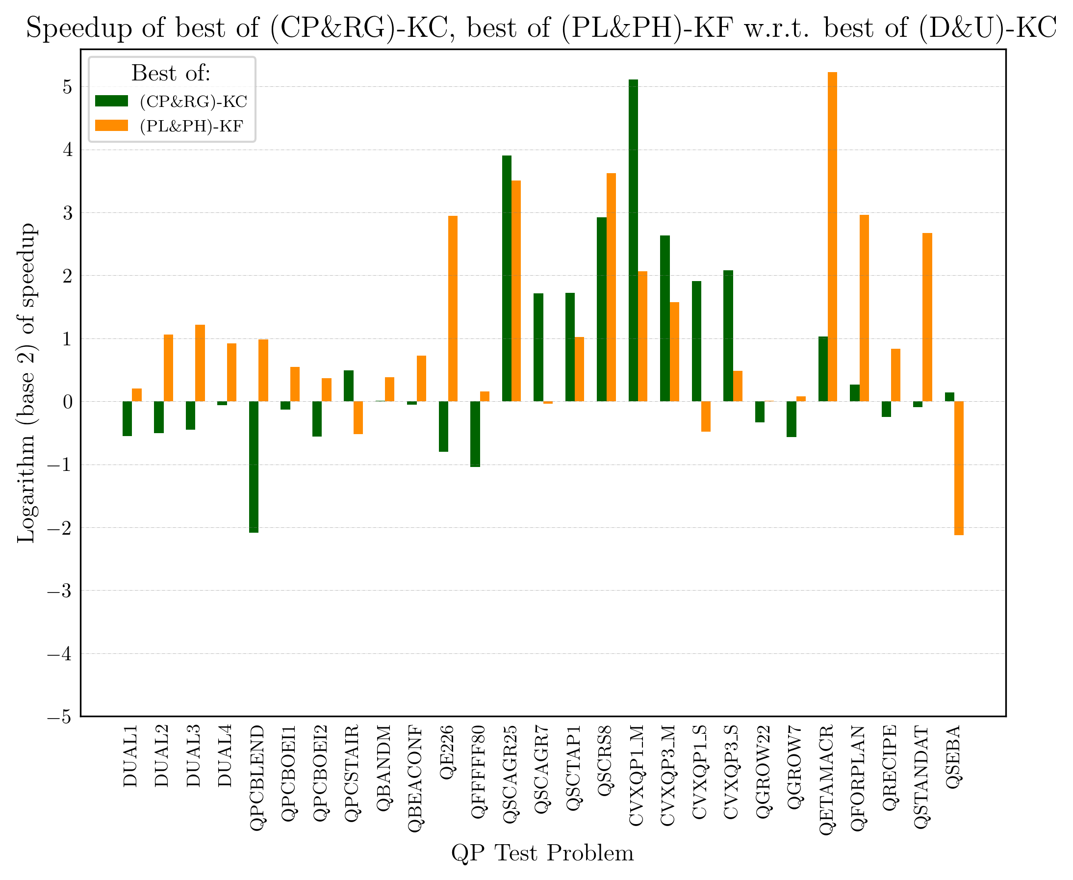
Excluding problems which are amenable to efficient direct solve (for which the direct solver D-KC is fastest among the variants) allows us to more clearly compare the performance among inexact IPM methods. We will denote this subset of problem as $\text{MMQP}_{\text{XD}}$ for the remainder of our experiments. Figure 5 shows the maximum speedup among the (CP-KC, RG-KC) variants, $\max\bigl{(}s_{CP-KC}^{D-U},s_{RG-KC}^{D-U}\bigr{)}$, and the (PL-KF, PH-KF) variants, $\max\bigl{(}s_{PL-KF}^{D-U},s_{PH-KF}^{D-U}\bigr{)}$, for the QP test problems for which at least one of the four variants has a speedup $s_{i}^{D-U}$ greater than $1$.

Comparing speed-ups across the $\text{MMQP}_{\text{XD}}$ subset of problems, the new preconditioned variants (PL&PH)-KF provide the lowest and most robust cost for the tested problems among alternative methods. Our preconditioned inexact IPM methods achieve a median speed-up of $1.8$ across this problem set in Fig. 5, compared to $0.9$ for the (CP&RG)-KC variants. Table 6 further shows that the PH-KF preconditioner is fastest for 59% of these problems, and taken together, either PL-KF or PH-KF is the method of choice for 2/3 of the problems.

Preconditioner	$p(\%)$	$\tilde{s}^{U}$	$\hat{s}^{U}$
PL-KF	7.41	4.89	4.58
PH-KF	59.25	25.16	34.08
CP-KC	29.63	14.79	18.24
RG-KC	3.7	2.97	3.53

Table 6: $p$ is the percentage of problems this preconditioner is the fastest among the four preconditioned variants for QP test problems (excluding problems where the direct method is the fastest). $\tilde{s}^{U}$ is the median speedup with respect to U-KC and $\hat{s}^{U}$ is the geometric mean speedup with respect to U-KC, across test problems where the direct method D-KC is not the fastest.

Figure 6: Speedups of PL-KF and PH-KF with respect to the fastest of the iterative augmented system variants (U-KC, CP-KC and RG-KC) for the $\text{MMQP}_{\text{XD}}$ problems for which the direct variant D-KF does not achieve the fastest overall.

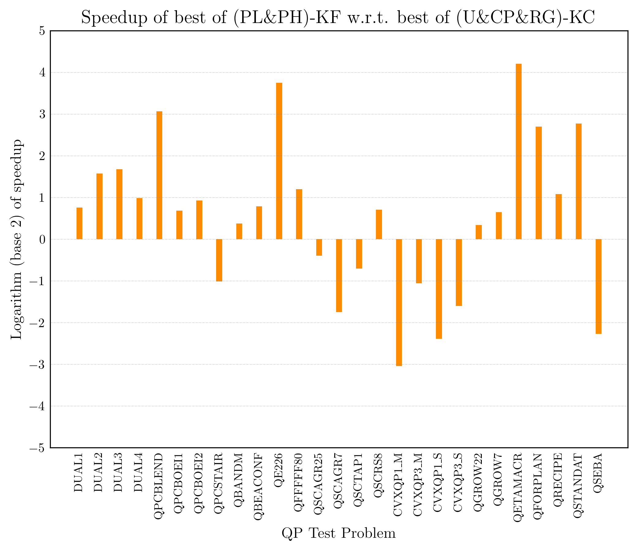
Lastly, we directly compare our IPM variants PL-KF and PH-KF, to the alternative iterative variants namely U-KC, CP-KC and RG-KC by computing the following speedup for QP test problems, once more excluding the ones agreeable with the direct solve variant,

(50) $$s_{\text{PL-PH}}^{\text{U-CP-RG}}(q_{j})=\frac{\min\bigl{(}c_{\text{U-KC}}(q_{j}),c_{\text{CP-KC}}(q_{j}),c_{\text{RG-KC}}(q_{j})\bigr{)}}{\min\bigl{(}c_{\text{PL-KF}}(q_{j}),c_{\text{PH-KF}}(q_{j})\bigr{)}},\;\;\;\;\;q_{j}\in{\{\text{MMQP}_{\text{XD}}\}}.$$

Figure 6 presents the logarithm (base 2) of these speedup (and slowdown) results. Our preconditioned inexact IPM solvers (PL&PH)-KF achieve a reduction in cost of $1.432$ (by geometric mean) relative to the best alternative inexact IPM variant.

7 Conclusion

Our theoretical analysis and experimental results demonstrate that the proposed new preconditioned iterative framework for IPM requires fewer iterations and minimal cost among alternatives in practical scenarios. For QP problems arising in particular applications, the structure of the Hessian and constraint matrices is often known, so a choice among methods should be guided by how much fill is expected in factorizations employed by each approach. Due to factorizing $K_{F}$, our inexact IPM solvers require that the KKT subsystem $F$ be nonsingular and that the fill in this factorization is manageable. In this paper, this invertibility is a enforced by a simple regularization, rendering the Hessian positive-definite. But an extension of our method to handle singular $H$ and/or $F$ is possible. In particular, if $H$ is singular, but $F$ is full rank, our approach is applicable except for the high-d.o.f. preconditioner, which would need to become more sophisticated. When $F$ is also singular, our method may be applied by taking the Schur complement of a smaller full-rank subsystem.

Our inexact IPM methods are a hybrid between direct and iterative solvers. The benefit of our approach with respect to a direct method is in avoiding the need to compute a matrix factorization at each IPM step and that the factorized matrix is independent of the inequality constraints. Relative to previously existing preconditioners, the preconditioned reduced system we employ is significantly better conditioned, which enables us to reduce iteration count and cost. The positive results obtained in our cost evaluations and conditioning studies suggest that a high-performance implementation of our method might achieve favorable performance to existing high-performance linear solvers for IPM.

QP Problem	$\min({\kappa}(\text{U}),{\kappa}(\text{CP}),{\kappa}(\text{RG}))$	$\min({\kappa}(\text{PL}),{\kappa}(\text{PH}))$	ratio
DUAL1	7.89e+02	2.16e+01	3.66e+01
DUAL2	2.14e+02	3.76e+00	5.70e+01
DUAL3	4.64e+02	2.89e+00	1.61e+02
DUAL4	6.48e+02	1.82e+00	3.56e+02
DUALC1	1.36e+09	7.89e+03	1.73e+05
DUALC5	1.46e+08	8.60e+02	1.70e+05
QPCBLEND	4.36e+11	5.60e+04	7.79e+06
QPCBOEI1	5.16e+07	6.43e+03	8.03e+03
QPCBOEI2	1.71e+08	1.05e+05	1.63e+03
QPCSTAIR	1.58e+07	4.81e+03	3.29e+03
QBANDM	3.64e+01	5.45e+06	6.68e-06
QADLITTL	3.42e+07	3.76e+06	9.11e+00
QAFIRO	3.35e+08	5.86e+03	5.71e+04
QBEACONF	3.70e+00	2.18e+09	1.70e-09
QE226	1.78e+09	9.79e+04	1.82e+04
QFFFFF80	1.30e+15	2.46e+08	5.28e+06
QSC205	2.30e+10	6.71e+04	3.43e+05
QSCAGR25	2.74e+07	2.32e+05	1.18e+02
QSCAGR7	1.85e+07	2.60e+05	7.13e+01
QSCFXM1	1.46e+11	1.41e+08	1.04e+03
QSCFXM2	1.73e+12	3.33e+08	5.20e+03
QSCTAP1	1.66e+08	5.39e+05	3.08e+02
QSHARE1B	4.79e+08	2.56e+07	1.87e+01
QSHARE2B	1.80e+09	2.56e+07	7.03e+01
QSCRS8	6.49e+12	2.77e+08	2.34e+04
CVXQP1_M	9.26e+05	6.89e+02	1.34e+03
CVXQP3_M	9.25e+06	4.99e+02	1.85e+04
CVXQP1_S	7.79e+05	8.99e+03	8.66e+01
CVXQP3_S	3.44e+06	4.02e+04	8.55e+01
QGROW15	4.68e+03	2.73e+03	1.71e+00
QGROW22	9.04e+03	2.09e+03	4.33e+00
QGROW7	9.50e+02	2.65e+03	3.59e-01
VALUES	2.39e+02	3.31e+03	7.22e-02
DUALC2	4.25e+09	4.55e+04	9.35e+04
DUALC8	1.65e+09	4.42e+03	3.73e+05
QETAMACR	4.28e+10	3.17e+07	1.35e+03
QFORPLAN	1.62e+13	1.98e+09	8.16e+03
QRECIPE	1.08e+08	1.35e+09	8.04e-02
QSTAIR	1.47e+07	7.76e+04	1.90e+02
QSTANDAT	1.14e+12	1.14e+10	9.96e+01
QSEBA	1.83e+06	8.99e+04	2.03e+01
Geometric mean over QP problems	3.13e+07	1.30e+05	2.40e+02

Table 7: Conditioning of the preconditioned augmented system and the preconditioned inequality constraint reduced system (with best choices of preconditioners for each), as well as the ratio of improvement obtained by the preconditioners, defined as $\min({\kappa}(\text{U}),{\kappa}(\text{CP}),{\kappa}(\text{RG}))/\min({\kappa}(\text{PL}),{\kappa}(\text{PH}))$.

References

- [1] G. Al-Jeiroudi, J. Gondzio, and J. Hall, Preconditioning indefinite systems in interior point methods for large scale linear optimisation, Optimisation Methods and Software, 23 (2008), pp. 345–363.
- [2] F. P. Ali Beik and M. Benzi, Iterative methods for double saddle point systems, SIAM Journal on Matrix Analysis and Applications, 39 (2018), pp. 902–921.
- [3] A. Altman and J. Gondzio, Regularized symmetric indefinite systems in interior point methods for linear and quadratic optimization, Optimization Methods and Software, 11 (1999), pp. 275–302.
- [4] M. Arioli, I. S. Duff, and P. P. de Rijk, On the augmented system approach to sparse least-squares problems, Numerische Mathematik, 55 (1989), pp. 667–684.
- [5] O. Axelsson and M. Neytcheva, Preconditioning methods for linear systems arising in constrained optimization problems, Numerical linear algebra with applications, 10 (2003), pp. 3–31.
- [6] R. E. Bank, B. D. Welfert, and H. Yserentant, A class of iterative methods for solving saddle point problems, Numerische Mathematik, 56 (1989), pp. 645–666.
- [7] S. Bellavia, Inexact interior-point method, Journal of Optimization Theory and Applications, 96 (1998), pp. 109–121.
- [8] S. Bellavia, V. De Simone, D. di Serafino, and B. Morini, Updating constraint preconditioners for KKT systems in quadratic programming via low-rank corrections, SIAM Journal on Optimization, 25 (2015), pp. 1787–1808.
- [9] M. Benzi and F. P. A. Beik, Uzawa-type and augmented lagrangian methods for double saddle point systems, in Structured Matrices in Numerical Linear Algebra, Springer, 2019, pp. 215–236.
- [10] M. Benzi, G. H. Golub, and J. Liesen, Numerical solution of saddle point problems, Acta numerica, 14 (2005), pp. 1–137.
- [11] M. Benzi and M. A. Olshanskii, An augmented lagrangian-based approach to the oseen problem, SIAM Journal on Scientific Computing, 28 (2006), pp. 2095–2113.
- [12] M. Benzi and A. J. Wathen, Some preconditioning techniques for saddle point problems, in Model Order Reduction: Theory, Research Aspects and Applications, Springer, 2008, pp. 195–211.
- [13] L. Bergamaschi, J. Gondzio, Á. Martínez, J. W. Pearson, and S. Pougkakiotis, A new preconditioning approach for an interior point-proximal method of multipliers for linear and convex quadratic programming, Numerical Linear Algebra with Applications, 28 (2021), p. e2361.
- [14] L. Bergamaschi, J. Gondzio, and G. Zilli, Preconditioning indefinite systems in interior point methods for optimization, Computational Optimization and Applications, 28 (2004), pp. 149–171.
- [15] S. Bocanegra, J. Castro, and A. R. Oliveira, Improving an interior-point approach for large block-angular problems by hybrid preconditioners, European Journal of Operational Research, 231 (2013), pp. 263–273.
- [16] Z.-H. Cao, Augmentation block preconditioners for saddle point-type matrices with singular (1, 1) blocks, Numerical Linear Algebra with Applications, 15 (2008), pp. 515–533.
- [17] L. Casacio, C. Lyra, A. R. L. Oliveira, and C. O. Castro, Improving the preconditioning of linear systems from interior point methods, Computers and Operations Research, 85 (2017), pp. 129–138.
- [18] E. Chow and Y. Saad, Approximate inverse techniques for block-partitioned matrices, SIAM Journal on Scientific Computing, 18 (1997), pp. 1657–1675.
- [19] H. S. Dollar, N. I. Gould, W. H. Schilders, and A. J. Wathen, Using constraint preconditioners with regularized saddle-point problems, Computational optimization and applications, 36 (2007), pp. 249–270.
- [20] M. D. Dražić, R. P. Lazović, and V. V. Kovačević-Vujčić, Sparsity preserving preconditioners for linear systems in interior-point methods, Computational Optimization and Applications, 61 (2015), pp. 557–570.
- [21] I. S. Duff, A. M. Erisman, and J. K. Reid, Direct methods for sparse matrices, Oxford University Press, 2017.
- [22] C. Durazzi and V. Ruggiero, Indefinitely preconditioned conjugate gradient method for large sparse equality and inequality constrained quadratic problems, Numerical linear algebra with applications, 10 (2003), pp. 673–688.
- [23] R. E. Ewing, R. D. Lazarov, P. Lu, and P. S. Vassilevski, Preconditioning indefinite systems arising from mixed finite element discretization of second-order elliptic problems, in Preconditioned conjugate gradient methods, Springer, 1990, pp. 28–43.
- [24] P. E. Farrell, L. Mitchell, and F. Wechsung, An augmented lagrangian preconditioner for the 3d stationary incompressible navier–stokes equations at high reynolds number, SIAM Journal on Scientific Computing, 41 (2019), pp. A3073–A3096.
- [25] R. Fletcher, Practical methods of optimization, John Wiley & Sons, 2013.
- [26] A. Forsgren, Inertia-controlling factorizations for optimization algorithms, Applied Numerical Mathematics, 43 (2002), pp. 91–107.
- [27] A. Forsgren, P. E. Gill, and J. D. Griffin, Iterative solution of augmented systems arising in interior methods, SIAM Journal on Optimization, 18 (2007), pp. 666–690.
- [28] A. Forsgren, P. E. Gill, and M. H. Wright, Interior methods for nonlinear optimization, SIAM review, 44 (2002), pp. 525–597.
- [29] M. Fortin and R. Glowinski, Augmented Lagrangian methods: applications to the numerical solution of boundary-value problems, Elsevier, 2000.
- [30] R. W. Freund, F. Jarre, and S. Mizuno, Convergence of a class of inexact interior-point algorithms for linear programs, Mathematics of Operations Research, 24 (1999), pp. 50–71.
- [31] R. W. Freund and N. M. Nachtigal, Software for simplified Lanczos and QMR algorithms, Applied Numerical Mathematics, 19 (1995), pp. 319–341.
- [32] W. N. Gansterer, J. Schneid, and C. W. Ueberhuber, Mathematical properties of equilibrium systems, tech. report, University of Vienna, 2003.
- [33] G. N. Gatica and N. Heuer, A dual-dual formulation for the coupling of mixed-fem and bem in hyperelasticity, SIAM Journal on Numerical Analysis, 38 (2000), pp. 380–400.
- [34] E. M. Gertz and S. J. Wright, Object-oriented software for quadratic programming, ACM Transactions on Mathematical Software (TOMS), 29 (2003), pp. 58–81.
- [35] P. E. Gill, W. Murray, D. B. Ponceleon, and M. A. Saunders, Solving reduced kkt systems in barrier methods for linear and quadratic programming, tech. report, STANFORD UNIV CA SYSTEMS OPTIMIZATION LAB, 1991.
- [36] P. E. Gill, W. Murray, D. B. Ponceleón, and M. A. Saunders, Preconditioners for indefinite systems arising in optimization, SIAM journal on matrix analysis and applications, 13 (1992), pp. 292–311.
- [37] P. E. Gill, W. Murray, D. B. Ponceleón, M. A. Saunders, G. Watson, and D. Griffiths, Solving reduced kkt systems in barrier methods for linear programming, Numerical Analysis, (1993), pp. 89–104.
- [38] R. Glowinski and P. Le Tallec, Augmented Lagrangian and operator-splitting methods in nonlinear mechanics, SIAM, 1989.
- [39] G. H. Golub and C. Greif, On solving block-structured indefinite linear systems, SIAM Journal on Scientific Computing, 24 (2003), pp. 2076–2092.
- [40] G. H. Golub and C. F. Van Loan, Matrix computations, vol. 3, JHU press, 2013.
- [41] J. Gondzio, Matrix-free interior point method, Computational Optimization and Applications, 51 (2012), pp. 457–480.
- [42] N. I. Gould, M. E. Hribar, and J. Nocedal, On the solution of equality constrained quadratic programming problems arising in optimization, SIAM Journal on Scientific Computing, 23 (2001), pp. 1376–1395.
- [43] N. I. Gould, D. Orban, and P. L. Toint, Cutest: a constrained and unconstrained testing environment with safe threads for mathematical optimization, Computational optimization and applications, 60 (2015), pp. 545–557.
- [44] C. Greif, G. H. Golub, and J. M. Varah, Augmented lagrangian techniques for solving saddle point linear systems, matrix, 500 (2004), pp. 1–1.
- [45] C. Greif, E. Moulding, and D. Orban, Bounds on eigenvalues of matrices arising from interior-point methods, SIAM Journal on Optimization, 24 (2014), pp. 49–83.
- [46] C. Greif and D. Schötzau, Preconditioners for saddle point linear systems with highly singular (1, 1) blocks, ETNA, Special Volume on Saddle Point Problems, 22 (2006), pp. 114–121.
- [47] C. Greif and D. Schötzau, Preconditioners for the discretized time-harmonic Maxwell equations in mixed form, Numerical Linear Algebra with Applications, 14 (2007), pp. 281–297.
- [48] J. C. Haws, Preconditioning KKT systems, PhD thesis, North Carolina State University, 2002.
- [49] E. V. Haynsworth and A. M. Ostrowski, On the inertia of some classes of partitioned matrices, Linear Algebra and its Applications, 1 (1968), pp. 299–316.
- [50] M. R. Hestenes, E. Stiefel, et al., Methods of conjugate gradients for solving linear systems, Journal of research of the National Bureau of Standards, 49 (1952), pp. 409–436.
- [51] C. Keller, N. I. Gould, and A. J. Wathen, Constraint preconditioning for indefinite linear systems, SIAM Journal on Matrix Analysis and Applications, 21 (2000), pp. 1300–1317.
- [52] P. Krzyzanowski, On block preconditioners for nonsymmetric saddle point problems, SIAM Journal on Scientific Computing, 23 (2001), pp. 157–169.
- [53] L. Lukšan and J. Vlček, Indefinitely preconditioned inexact newton method for large sparse equality constrained non-linear programming problems, Numerical linear algebra with applications, 5 (1998), pp. 219–247.
- [54] I. J. Lustig, R. E. Marsten, and D. F. Shanno, On implementing Mehrotra’s predictor–corrector interior-point method for linear programming, SIAM Journal on Optimization, 2 (1992), pp. 435–449.
- [55] K.-A. Mardal and R. Winther, Uniform preconditioners for the time dependent stokes problem, Numerische Mathematik, 98 (2004), pp. 305–327.
- [56] I. Maros and C. Mészáros, A repository of convex quadratic programming problems, Optimization Methods and Software, 11 (1999), pp. 671–681.
- [57] M. D. Mihajlović and D. J. Silvester, Efficient parallel solvers for the biharmonic equation, Parallel Computing, 30 (2004), pp. 35–55.
- [58] B. Morini, V. Simoncini, and M. Tani, Spectral estimates for unreduced symmetric kkt systems arising from interior point methods, Numerical Linear Algebra with Applications, 23 (2016), pp. 776–800.
- [59] B. Morini, V. Simoncini, and M. Tani, A comparison of reduced and unreduced KKT systems arising from interior point methods, Computational Optimization and Applications, 68 (2017), pp. 1–27.
- [60] J. Nocedal and S. J. Wright, Numerical Optimization, Springer, New York, NY, USA, second ed., 2006.
- [61] A. R. Oliveira and D. C. Sorensen, A new class of preconditioners for large-scale linear systems from interior point methods for linear programming, Linear Algebra and its applications, 394 (2005), pp. 1–24.
- [62] C. C. Paige and M. A. Saunders, Solution of sparse indefinite systems of linear equations, SIAM journal on numerical analysis, 12 (1975), pp. 617–629.
- [63] J. W. Pearson and J. Gondzio, Fast interior point solution of quadratic programming problems arising from pde-constrained optimization, Numerische Mathematik, 137 (2017), pp. 959–999.
- [64] J. W. Pearson and J. Pestana, Preconditioners for krylov subspace methods: An overview, GAMM-Mitteilungen, 43 (2020), p. e202000015.
- [65] I. Perugia and V. Simoncini, Block-diagonal and indefinite symmetric preconditioners for mixed finite element formulations, Numerical linear algebra with applications, 7 (2000), pp. 585–616.
- [66] S. Pougkakiotis and J. Gondzio, Dynamic non-diagonal regularization in interior point methods for linear and convex quadratic programming, Journal of Optimization Theory and Applications, 181 (2019), pp. 905–945.
- [67] S. Pougkakiotis and J. Gondzio, An interior point-proximal method of multipliers for convex quadratic programming, Computational Optimization and Applications, 78 (2021), pp. 307–351.
- [68] C. E. Powell and D. Silvester, Optimal preconditioning for raviart–thomas mixed formulation of second-order elliptic problems, SIAM journal on matrix analysis and applications, 25 (2003), pp. 718–738.
- [69] A. Ramage and E. C. Gartland Jr, A preconditioned nullspace method for liquid crystal director modeling, SIAM Journal on Scientific Computing, 35 (2013), pp. B226–B247.
- [70] T. Rees and C. Greif, A preconditioner for linear systems arising from interior point optimization methods, SIAM Journal on Scientific Computing, 29 (2007), pp. 1992–2007.
- [71] M. Rozlozník and V. Simoncini, Krylov subspace methods for saddle point problems with indefinite preconditioning, SIAM Journal on Matrix Analysis and Applications, 24 (2002), pp. 368–391.
- [72] Y. Saad, Iterative methods for sparse linear systems, SIAM, 2003.
- [73] Y. Saad and M. H. Schultz, GMRES: A generalized minimal residual algorithm for solving nonsymmetric linear systems, SIAM Journal on scientific and statistical computing, 7 (1986), pp. 856–869.
- [74] M. A. Saunders et al., Cholesky-based methods for sparse least squares: The benefits of regularization, Linear and nonlinear conjugate gradient-related methods, 100 (1996), pp. 92–100.
- [75] S.-Q. Shen, T.-Z. Huang, and J.-S. Zhang, Augmentation block triangular preconditioners for regularized saddle point problems, SIAM Journal on Matrix Analysis and Applications, 33 (2012), pp. 721–741.
- [76] D. Silvester and A. Wathen, Fast iterative solution of stabilised stokes systems part ii: Using general block preconditioners, SIAM Journal on Numerical Analysis, 31 (1994), pp. 1352–1367.
- [77] J. Sogn and W. Zulehner, Schur complement preconditioners for multiple saddle point problems of block tridiagonal form with application to optimization problems, IMA Journal of Numerical Analysis, 39 (2019), pp. 1328–1359.
- [78] K.-C. Toh, K.-K. Phoon, and S.-H. Chan, Block preconditioners for symmetric indefinite linear systems, International Journal for Numerical Methods in Engineering, 60 (2004), pp. 1361–1381.
- [79] Z. Tong and A. Sameh, On an iterative method for saddle point problems, Numerische Mathematik, 79 (1998), pp. 643–646.
- [80] H. A. Van der Vorst, Bi-CGSTAB: A fast and smoothly converging variant of Bi-CG for the solution of nonsymmetric linear systems, SIAM Journal on scientific and Statistical Computing, 13 (1992), pp. 631–644.
- [81] L. Vandenberghe, The cvxopt linear and quadratic cone program solvers, Online: http://cvxopt. org/documentation/coneprog. pdf, (2010).
- [82] A. Wächter and L. T. Biegler, On the implementation of an interior-point filter line-search algorithm for large-scale nonlinear programming, Mathematical programming, 106 (2006), pp. 25–57.
- [83] W. Wang and D. P. O’Leary, Adaptive use of iterative methods in predictor–corrector interior point methods for linear programming, Numerical Algorithms, 25 (2000), pp. 387–406.
- [84] A. Wathen, B. Fischer, and D. Silvester, The convergence rate of the minimal residual method for the stokes problem, Numerische Mathematik, 71 (1995), pp. 121–134.
- [85] M. H. Wright, Interior methods for constrained optimization, Acta numerica, 1 (1992), pp. 341–407.
- [86] S. J. Wright, Primal-dual interior-point methods, SIAM, 1997.
- [87] Y. Zhang, Solving large-scale linear programs by interior-point methods under the MATLAB environment, Optimization Methods and Software, 10 (1998), pp. 1–31.