Energy Savings by Task Offloading to a Fog Considering Radio Front-End Characteristics

Abstract

Fog computing can be used to offload computationally intensive tasks from battery powered Internet of Things (IoT) devices. Although it reduces energy required for computations in an IoT device, it uses energy for communications with the fog. This paper analyzes when usage of fog computing is more energy efficient than local computing. Detailed energy consumption models are built in both scenarios with the focus set on the relation between energy consumption and distortion introduced by a Power Amplifier (PA). Numerical results show that task offloading to a fog is the most energy efficient for short, wideband links.

I Introduction

Cloud computing has become an established paradigm to provide various services to end users, e.g., computational resources for IoT devices [1]. The cloud is typically located hundreds of kilometers away from the end device [2]. The corresponding communications delay and jitter can be therefore significant. Fog computing, being set of computational resources (e.g., local servers, small data centers) located close to the end user, has been introduced to address this problem [3]. At the same time fog computing can reduce required local computing and therefore simplify IoT end devices construction and cost. At the same time the power required for computations at IoT devices is reduced. Optimization of IoT devices Energy Efficiency (EE) is particularly important when these devices are battery powered.

Research on green fog networks is usually focused on delay and energy efficiency of computations carried in fog instead of the cloud [4, 5]. Modelling of energy consumption of the fog network as a whole is performed in [6, 5, 4]. However, energy consumption modeling of mobile devices is omitted. On the other hand, there are articles focused on energy consumption of mobile/IoT devices in fog computing environment. In [7] offloading decisions of a single mobile device are examined. In [8, 9, 10] optimization of offloading decisions of multiple mobile devices is performed jointly. Energy consumption spent on local computations and transmission is considered in [8, 9, 7]. Additionally, energy spent on computations in Fog Nodes is considered in [10]. However, models of energy consumption for transmission used in each of these papers are simple and do not cover BaseBand (BB) and Radio Frequency (RF) processing required to transmit data. To the best of our knowledge, our work is the first one to cover these aspects in the context of fog networks.

Our research question is formulated as follows: when is it beneficial to offload computations to the fog from the perspective of energy consumption of an IoT device? Both solutions, i.e., local computations and data offloading consume various amounts of energy. Energy required to process data locally is compared with energy required for preparation and sending data to the fog. Accurate modelling of wireless transmission costs is essential to properly assess the viability of offloading computations to the fog tier. First, we provide detailed models of power spent by end devices on transmission. The radio transmission chain is divided into separate elements. Significant attention is devoted to power consumption and nonlinear distortion introduced by a PA. It can consume significant amount of power and introduce significant distortion [11, 12, 13]. Both effects are modeled considering soft limiter nonlinearity model and power consumption of class B PA. Second, the optimal operating point of the PA is derived and used assuming Signal-to-Interference and Noise Ratio (SINR) maximization. We take video surveillance as an application scenario. It consists of one or multiple IoT devices, i.e., high-bitrate cameras utilizing Time-Division Multiple Access (TDMA). We assume Orthogonal Frequency-Division Multiplexing (OFDM) for transmission which is a state-of-the-art technology in modern wireless communications, e.g, used in WiFi and Long Term Evolution (LTE). Our results confirm that the PA consumes significant part of link power. This is particularly evident for long distances and narrow transmission bandwidths. Fog computing is the most advantageous for short links with wide bandwidth available. To the best of our knowledge, this work is the first one to consider detailed power model of an IoT device in the context of offloading computations to fog or performing them locally.

The rest of this paper is organized as follows. The considered fog network architecture is presented in Sec. II along with the system model including the power consumption model of the local computations as well as in the case of offloading computations to the Fog. Sec. III details numerical results. The paper is summarized in Sec. IV.

II Fog application for video surveillance

We use the fog architecture shown in Fig. 1. It consists of three tiers. The Things tier includes IoT devices. These devices are sources of computation requests. The requests can be served either locally, or offloaded using a wireless connection to the Fog tier, i.e., a nearby Base Station (BS). The BS has a short-range wired connection to a FN which can process computational tasks sent by IoT devices. In addition, some computationally intensive and delay tolerant tasks can be sent to a far-away Cloud tier or distributed among many FNs.

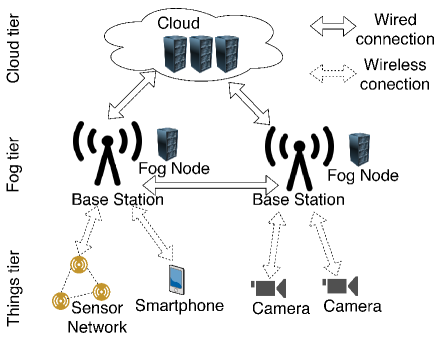
Figure 1: The considered fog network architecture.

In our application system, we consider $M$ video cameras, each generating constant bitrate stream that has to be processed requiring high computational load. Face recognition is an exemplary application.

II-A Local computations

In the case of local computations, the power consumption can be modeled as a function of clock frequency, voltage, and some platform specific coefficients [14]. However, such a model is not directly related to the computational power measured in number of Floating point Operations Per Second (FLOPS) available. Therefore, here, a mean, constant processing efficiency of $\Gamma=5\textrm{ }GFLOPS/W$ is used as in [15]. It is inline with values reported for some smartphones, e.g., Samsung Galaxy S6 [16]. The total power consumption for local calculations $P_{local}$ is defined as

$$P_{local}=\frac{\theta\cdot R}{\Gamma}\text{,}$$ (1)

where $R$ denotes the bitrate of video stream after compression while $\theta$ is the computational complexity coefficient determining the mean number of operations per single encoded bit required to complete the task, e.g., face recognition. Thus, $\theta\cdot R$ specifies the required computational load in FLOPS.

II-B Offloading to the Fog

The workload $\theta\cdot R$ can be offloaded to the fog network reducing energy consumption of the local device. On the other hand, the task offloading requires the data to be transmitted via the network to the fog. This forms another source of energy consumption. The data offloading is carried in Up Link (UL) of OFDM-based system (being a common choice for modern wireless communications systems). The downlink is neglected as a few orders of magnitude lower throughput is usually experienced. All $M$ cameras are sharing resources of a single serving BS, utilizing $1/M$-th of available time resources. TDMA is the most energy efficient approach for sharing transmission media [11]. According to [17] the UL rate considering adaptive modulation and coding can be approximated by the scaled Shannon formula

$$R=\beta\frac{B}{M}\log_{2}\left(1+SINR\right)\text{,}$$ (2)

where $B$ is the useful bandwidth of the transmitted signal, SINR is Signal-to-Interference and Noise Ratio, and $\beta$ is a scaling coefficient. In [17] $\beta$ is equal 0.55 assuming Single-Input Single-Output (SISO) transmission in Additive White Gaussian Noise (AWGN) channel and 0.4 assuming Single-Input Multiple-Output (SIMO) transmission in UL of typical urban fast fading channel.

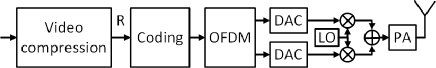
Figure 2: Diagram of the considered IoT transmitter.

The diagram of the considered transmitter is shown in Fig. 2. The stream of bitrate $R$ is encoded and modulated (with power consumption detailed in Sec. II-B2) and transmitted using many subcarriers using OFDM (resulting in power consumption described in Sec. II-B3). The complex symbols at the output of OFDM block are separated to in-phase and quadrature phase real symbols and fed to two Digital-Analog Converters of $N_{\mathrm{DAC}}$ bit resolution and conversion speed $f_{s}$, where $f_{s}>B$. The considered DAC power consumption model is provided in Sec. II-B4. In order to reduce power consumption Zero- Intermediate Frequency (IF) architecture is considered as in [12] requiring in addition only one Local Oscillator (LO) and two mixers whose power consumption models are provided in Sec. II-B5 and Sec. II-B6, respectively. Finally, the signal at radio frequency has to be amplified in PA and fed to the antenna.

In the simplest approach the higher the transmit power, the higher the received power and higher the achievable link throughput. However, nonlinear distortion of OFDM signal passing through PA has to be considered[11]. The OFDM signal samples $x$ for sufficiently high number of subcarriers follow complex-Gaussian distribution [18]. Assuming that the PA can be modeled in BB as a soft limiter with the input OFDM signal $x\sim\mathcal{CN}(0,\sigma^{2})$, the output sample $\tilde{x}$ equals:

$$\tilde{x}=\begin{cases}x&\mbox{for}~{}~{}|x|<\sqrt{P_{\mathrm{MAX}}}\\ \frac{\sqrt{P_{\mathrm{MAX}}}}{|x|}x&\mbox{for}~{}~{}|x|\geq\sqrt{P_{\mathrm{MAX}}},\end{cases}$$ (3)

where $P_{\mathrm{MAX}}$ is the maximum power of a sample, i.e., clipping threshold. An Input Back-Off (IBO) defined as

$$\mathrm{IBO}=\frac{P_{\mathrm{MAX}}}{\sigma^{2}}$$ (4)

is a common measure of PA operating point, i.e., how far the mean transmission power is from the clipping power. The energy consumption of a PA is discussed in Sec. II-B7. According to the Bussgang theorem the nonlinearly distorted signal can be decomposed into linearly down-scaled (by coefficient $\alpha$ defined in [19]) input signal and uncorrelated distortion $n_{\mathrm{PA}}$, i.e.,

$$\tilde{x}=\alpha x+n_{\mathrm{PA}}.$$ (5)

This signal reaches a receiver being attenuated by the channel of a single coefficient $h$ (reflecting path loss; other effects like fading are included in coefficient $\beta$), where the noise sample $n_{\mathrm{RX}}\sim\mathcal{CN}(0,N)$ is added, resulting in

$$\tilde{y}=h\alpha x+hn_{\mathrm{PA}}+n_{\mathrm{RX}}.$$ (6)

Based on derivations in [19, 11] it can be shown that the received SINR value equals

$$SINR =\frac{|h|^{2}\alpha^{2}\sigma^{2}}{|h|^{2}\mathbb{E}\left[|n_{\mathrm{PA}}|^{2}\right]+N}$$ (7)

$$=\frac{\alpha^{2}}{1-\alpha^{2}-e^{-\mathrm{IBO}}+\frac{IBO}{SNR_{\mathrm{MAX}}}},$$

where $\alpha=1-e^{-\mathrm{IBO}}+0.5\sqrt{\pi\mathrm{IBO}}\mathrm{erfc}\left(\sqrt{\mathrm{IBO}}\right)$ and $SNR_{\mathrm{MAX}}=|h|^{2}P_{\mathrm{MAX}}/N$. SINR depends on IBO and $SNR_{\mathrm{MAX}}$ that can be interpreted as maximum possible SINR that can be obtained if input signal $x$ is a complex sine of power $P_{\mathrm{MAX}}$ resulting in no nonlinear distortion but maximum PA utilization. For SINR maximization, the optimal IBO value can be derived (as shown in Appendix A) by numerically solving (e.g., using the Newton method) the following equation

$$\frac{\sqrt{\pi}}{2}\mathrm{erfc}\left(\sqrt{\mathrm{IBO}}\right)=\frac{\sqrt{\mathrm{IBO}}}{SNR_{\mathrm{MAX}}}.$$ (8)

The resulting IBO value (see (7)) is shown in Fig. 3 for $(SNR_{\mathrm{MAX}})_{dB}\in\langle-10,50\rangle$. Most interestingly, the maximum SINR can be approximated in dB scale as

$$(SINR)_{dB}\approx 0.84(SNR_{\mathrm{MAX}})_{dB}-2.23$$ (9)

with maximum error lower than 0.5 dB for $(SNR_{\mathrm{MAX}})_{dB}\in\langle-10,50\rangle$ as shown in Fig. 3.

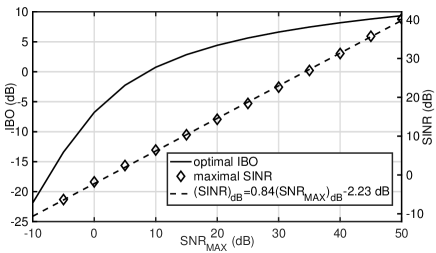
Figure 3: Optimal IBO and SINR value for SINR maximization vs. $SNR_{\mathrm{MAX}}$ value.

For a known bitrate requirement $R$, SINR calculated from (2) can be used in (9) giving

$$0.84(SNR_{\mathrm{MAX}})_{dB}-2.23=10\log_{10}\left(2^{\frac{MR}{\beta B}}-1\right).$$ (10)

After some simplifications and substitution of the $SNR_{\mathrm{MAX}}$ definition we obtain:

$$P_{\mathrm{MAX}}=\frac{N}{|h|^{2}}10^{\frac{1}{0.84}\log_{10}\left(2^{\frac{MR}{\beta B}}-1\right)+\frac{2.23}{10\cdot 0.84}}.$$ (11)

The last equation determines optimum (maximizing SINR over IBO) clipping power of the PA that influences power utilization described in Sec. II-B7.

The mean power consumption of a single camera for the task offloading to the fog $P_{\mathrm{off.}}$ is given as

$$P_{\mathrm{off.}}= P_{\mathrm{VIDEO}}+P_{\mathrm{COD}}+\frac{1}{M}P_{\mathrm{OFDM}}+\frac{2}{M}P_{\mathrm{DAC}}+$$

$$+P_{\mathrm{LO}}+\frac{2}{M}P_{\mathrm{MIX}}+\frac{1}{M}P_{\mathrm{PA}},$$ (12)

where $P_{\mathrm{VIDEO}}$, $P_{\mathrm{COD}}$, $P_{\mathrm{OFDM}}$, $P_{\mathrm{DAC}}$, $P_{\mathrm{LO}}$, $P_{\mathrm{MIX}}$, and $P_{\mathrm{PA}}$ denote power consumed by video coder, redundancy coding, OFDM, DAC, LO, mixer, and PA, respectively. Division by $M$ is carried for transmitter components that are turned off when other cameras transmit their data, i.e., a component is active only $1/M$-th of time. They are detailed in the sections below.

II-B1 Video compression

In order to transmit a video signal its raw video frames have to be encoded. H264 is one of the state-of-the-art compression standards that can be used for this purpose. Video encoding is a computationally intensive process. This fact together with high popularity of watching videos leads to high availability of dedicated Application-Specific Integrated Circuits in the mass market [20]. The power consumption depends on many parameters including coder configuration, resolution, and utilized Complementary Metal-Oxide-Semiconductor (CMOS) technology. Average power consumption is reported in [20], e.g., $P_{\mathrm{VIDEO}}=242\textrm{ }mW$ for a Full HD stream. The typical output bitrate is $R=6\textrm{ }Mbps$.

II-B2 Redundancy coding

The source encoded data has to be protected from transmission errors by redundancy coding, e.g., turbo or Low-Density Parity Check (LDPC). Typically, the power utilized by the coder $P_{\mathrm{COD}}$ is proportional to the bitrate $R$ [12, 15, 11]. We assume the proportionality factor $\psi=0.1$ W/Gbps [15] in this work , i.e., $P_{\mathrm{COD}}=R\cdot\psi$.

II-B3 OFDM

The computational complexity of an OFDM transmitter is dominated by Inverse Fast Fourier Transform (IFFT) [21]. For a given transmitter bandwidth (not useful band spanned by utilized subcarriers), a subcarrier bandwidth of $\Delta f$ can be assumed giving IFFT size $N_{OFDM}=f_{s}/\Delta f$.

Assuming the number of operations required for IFFT equals $4N_{OFDM}\log_{2}(N_{OFDM})-6N_{OFDM}+8$ [21] and constant OFDM symbol duration equal to $1/\Delta f$ (the cyclic prefix duration is neglected for simplicity) the required computational complexity equals $(4N_{OFDM}\log_{2}(N_{OFDM})-6N_{OFDM}+8)\Delta f$ FLOPSs. We use $\Gamma_{MOD}$ being a constant number of operations per second per Watt to map the computational complexity to power consumption. A value of $\Gamma_{MOD}=120~{}GFLOPS/W$ is assumed for femto base stations [12]. This value can be much higher than $\Gamma$ reported for general purpose processors as the computing unit can be optimized specifically for this task. This is related also to the utilized terminal, i.e., $P_{\mathrm{OFDM}}=\left(4N_{OFDM}\log_{2}(N_{OFDM})-6N_{OFDM}+8\right)\Delta f\cdot\frac{1}{\Gamma_{MOD}}$.

II-B4 Digital-Analog Converter

The power consumption $P_{\mathrm{DAC}}$ (in Watts) of a DAC is modeled as in [13] as

$$P_{\mathrm{DAC}}=V_{dd}I_{0}\left(2^{N_{\mathrm{DAC}}}-1\right)+0.5N_{\mathrm{DAC}}C_{p}f_{s}V_{dd}^{2},$$ (13)

where $V_{dd}$ denotes power supply voltage (3 V following [13]), $I_{0}$ denotes unit current per least significant bit ($5\text{ }\mu A$ [13]), $N_{\mathrm{DAC}}$ is resolution in bits of DAC (10 bits), and $C_{p}$ is parasitic capacitance ($1\text{ }pF$ [13]).

II-B5 Local Oscillator

Real implementations of local oscillators are reported in [22, 13]. We assume constant power consumption of the local oscillator $P_{\mathrm{LO}}=67.5\textrm{ }[mW]$ based on [13].

II-B6 Mixer

A Zero-IF transmitter uses two mixers: one for the in-phase component and one for the quadrature component. Based on [13] a constant value of $P_{\mathrm{MIX}}=21\textrm{ }[mW]$ is used here for one mixer.

II-B7 PA

Modeling of power consumed by a PA is a complex task depending on several factors such as PA class, input signal distribution and specific implementation [23]. A class B PA is considered in [11] as it provides relatively high energy efficiency (up to 78.5%) and has relatively simple construction that is suitable for mobile devices. Similarly, in [24] l-way Doherty PA is assumed being generalization of B class PA. However, while [11] does not consider input signal clipping (required by the considered soft limiter PA model), [24] does not consider OFDM samples power distribution. Therefore, the class B PA power consumption $P_{\mathrm{PA}}$ assuming soft limiter nonlinear characteristic for complex Gaussian input signal is derived in Appendix B giving:

$$P_{\mathrm{PA}}=\frac{2P_{\mathrm{MAX}}}{\sqrt{\pi IBO}}\mathrm{erf}\left(\sqrt{IBO}\right),$$ (14)

where optimal IBO is calculated solving (8) for $SNR_{\mathrm{MAX}}$ from (9) and $P_{\mathrm{MAX}}$ is calculated based on (11).

III Numerical results

The considered IoT link offloading computations to the fog is analyzed using parameters summarized in Table I. The propagation channel amplification $10\log_{10}\left(|h|^{2}\right)$ assumes path loss for macro, urban base station, with 0 dBi IoT device gain and 15 dBi base station antenna gain [17]. Distance between base station and IoT device is $d$ (in km) and carrier frequency is denoted by $f$. Noise power $N$ is modeled as thermal noise in $20^{o}C$ increased by 5 dB noise figure according to [17].

TABLE I: Parameters used in numerical evaluation.

Parameter	Value
$\Gamma$	5 GFLOPS/W [15]
$\beta$	0.4 [17]
R	6 Mbit/s
$M$	$\{1;10\}$
$P_{VIDEO}$	242 mW [20]
$f_{s}$	$\{15.36;30.72\}$ MHz [17]
$B$	$\{9;18\}$ MHz [17]
$N_{OFDM}$	$\{1024;2048\}$ [17]
$\Gamma_{MOD}$	120 GFLOPS/W [12]
$\Delta f$	15 kHz
$f$	3.5 GHz
$10\log_{10}\left(|h|^{2}\right)$	$15\!-\!\Bigl{(}\!128.1\!+\!37.6log_{10}(d\text{ }[km])\!+$
	$+\!21log_{10}\left(\frac{f}{2\text{ }[GHz]}\right)\Bigr{)}$ [17]
$(N)_{dBm}$	$-174+10log_{10}(B)+5$ dBm [17]
$P_{LO}$	67.5 mW [13]
$P_{MIX}$	21 mW [13]
$P_{COD}$	$0.1\cdot R$ [mW/Mbps] [15]
$V_{DD}$	$3\text{ }V$[13]
$I_{0}$	$5\text{ }\mu A$[13]
$C_{p}$	$1\text{ }pF$[13]
$N_{DAC}$	10 bit

The optimal SINR changes according to (2) as shown in the top part of Fig. 4 under varying utilized bandwidth and fixed rate $R=6\text{ }Mbps$. Higher bandwidth allows the same rate to be achieved by lower SINR. Higher number of cameras sharing spectrum require higher SINR as well. The SINR can be used to calculate optimal parameters of the PA, i.e., $SNR_{MAX}$ using (9) and IBO using (8) presented in the bottom of Fig. 4. The optimal IBO (maximizing SINR defined by (7)) decreases with available bandwidth achieving IBO lower than 0 dB for B greater than 7 MHz and $M=1$. Such low setting of IBO results in relatively high PA energy efficiency at the cost of relatively high nonlinear distortion power.

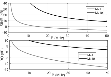
Figure 4: Optimal SINR and IBO for given bandwidth $B$ and constant rate $R=6\text{ }Mbps$.

The required power for offloading the video stream to the fog for processing is shown in Fig. 5 for varying distance between IoT device and base station. Two transmission bandwidths and 1 or 10 cameras are considered. The power consumption for short distance communications (e.g., below 20 m) equals around 26 dBm (differences below 1 dB) in each case. This is dominated by components other than PA. Video compression consumes around 24 dBm. This is inline with power consumption of WiFi cards reported in [25] where a significant constant, idle power is visible. However, as the communications link becomes longer, the PA power consumption becomes dominant over all power consumption components. This phenomenon is particularly significant for narrow bandwidth and high number of cameras sharing the radio channel.

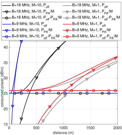
Figure 5: Power required for offloading vs. distance and available bandwidth.

Finally, the power consumed by an IoT device for local computing is compared with power consumed by the same device for communications performed to offload the computation task to the fog in Fig. 6. The total communications power $P_{off.}$ is compared with (1) in order to obtain the maximum number $\theta$ of FLOPS per bit of compressed video stream that can be carried locally within the same power budget. For short links (distance below 20 m) it is more power efficient to offload tasks to the fog if $\theta$ is greater than 320 FLOP/bit and 267 FLOP/bit for $M=1$ and $M=10$, respectively. For longer distance the computations complexity coefficient $\theta$ has to be even higher to offload the task, e.g., for $d=1000\textrm{ }m$ and one camera it equals around 620 FLOP/bit and 530 FLOP/bit for $B=$ 9 MHz and 18 MHz, respectively. These numbers are significantly higher for 10 cameras sharing radio channel. Maximal $\theta$ is lower for $M=10$ than for $M=1$ at distances lower than 200 m. This is due to the fact that PA power is low for low distances. The constant terms from (12) dominate $P_{off.}$ then. Some elements (such as mixers or DACs) can be switched off when the number of devices $M$ is bigger than 1 (see the divisions over $M$ in (12)).

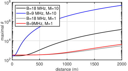
Figure 6: Maximal number of floating point operations per encoded video bit making local computations more power efficient.

IV Conclusions

In the context of ever lacking energy stored in the batteries of mobile IoT devices, we answer the question whether it is beneficial from the power consumption perspective to perform computations locally by the IoT device or to offload (i.e., send) them to the fog. We contribute with a detailed power consumption model of IoT device for data offloading to the fog and local computations. Optimal operating point of the PA is derived and used assuming SINR maximization. The results prove that usage of fog computing reduces IoT device power consumption mostly for short transmission distances, wide transmission bandwidth, and relatively high local computations complexity, e.g., more than 300 FLOP per bit of compressed video stream. Numerical values are valid for the considered, realistic system parameters. The general trend is expected to be valid for most setups. Verification of the analytical results against measurements of equipment on a testbed or in a real fog network would be useful in the future. An algorithm deciding when to offload computations to the fog is also needed.

Appendix A Optimal IBO for SINR maximization

The IBO maximizing SINR in (7) can be calculated by finding $z=\sqrt{IBO}$ for which SINR derivative equals 0, i.e.,

$$\frac{\partial SINR}{\partial z}=\frac{2\alpha}{\left(1-\alpha^{2}-e^{-z^{2}}+\frac{z^{2}}{SNR_{\mathrm{MAX}}}\right)^{2}}\cdot$$ (15)

$$\cdot\left(\frac{\partial\alpha}{\partial z}\left(\!1\!\!-\!\!e^{-z^{2}}\!\!+\!\!\frac{z^{2}}{SNR_{\mathrm{MAX}}}\!\!\right)\!-\alpha ze^{-z^{2}}\!\!-\!\frac{\alpha z}{SNR_{\mathrm{MAX}}}\right)\!=\!0,$$

where $\frac{\partial\alpha}{\partial z}=ze^{-z^{2}}+\frac{\sqrt{\pi}}{2}\mathrm{erfc}\left(z\right)$. Observing that the denominator is always positive, the root of the nominator has to be found. The following equation is obtained after omission of denominator and substitution of $\frac{\partial\alpha}{\partial z}$ and $\alpha$:

$$\left(\!1\!-\!e^{-z^{2}}\!-\!z^{2}e^{-z^{2}}\right)\left(\frac{\sqrt{\pi}}{2}\mathrm{erfc}\left(z\right)-\frac{z}{SNR_{\mathrm{MAX}}}\right)=0.$$ (16)

In the above product the first factor is always positive for $z>0$. This stems from the fact that it equals 0 for $z=0$ and its derivative, i.e., $2z^{3}e^{-z^{2}}$, is positive for any $z>0$. Therefore, the second factor has to be equal 0 resulting in (8).

Appendix B Class B PA power consumption for complex Gaussian input signal

For the input PA signal $x$ the output signal $\tilde{x}$, described by (3), achieves maximum power $P_{\mathrm{MAX}}$. Consumed power $\hat{P}_{\mathrm{PA}}$ of a class B PA transmitting sine wave of mean power $p$ is given as

$$\hat{P}_{\mathrm{PA}}=\frac{4}{\pi}\sqrt{pP_{\mathrm{MAX}}}$$ (17)

following [23, 11]. It has to be averaged over experienced instantaneous power distribution for any other transmitted signal. Each OFDM symbol sample $x$ can be well approximated by a complex normal distribution with variance $\sigma^{2}$, i.e., $x\sim\mathcal{CN}(0,\sigma^{2})$. Therefore, amplitude $z=|x|$ is Rayleigh distributed with parameter $\sigma/\sqrt{2}$ resulting in probability density function

$$f_{z}(z)=\frac{2z}{\sigma^{2}}\exp{\left(-\frac{z^{2}}{\sigma^{2}}\right)}.$$ (18)

The mean PA power consumption is calculated as follows:

$$P_{\mathrm{PA}}=E\left[\hat{P}_{\mathrm{PA}}\right]=\frac{4}{\pi}\sqrt{P_{\mathrm{MAX}}}\int_{0}^{\infty}\left|\tilde{x}\right|f_{z}(z)dz.$$ (19)

It can be rewritten utilizing (3) as

$$P_{\mathrm{PA}}=\frac{4}{\pi}\sqrt{P_{\mathrm{MAX}}}\left(\int_{0}^{\sqrt{P_{\mathrm{MAX}}}}\!\!\!\!\!\!\!\!\!\!\!\!\!\!\!\!\!zf_{z}(z)dz+\int_{\sqrt{P_{\mathrm{MAX}}}}^{\infty}\!\!\!\!\!\!\!\!\!\!\!\!\sqrt{P_{\mathrm{MAX}}}f_{z}(z)dz\right).$$ (20)

It can be found that

$$\int\frac{z^{2}}{B}\exp{\left(-\frac{z^{2}}{B}\right)}dz=\frac{\sqrt{\pi B}}{4}\mathrm{erf}\left(\frac{z}{\sqrt{B}}\right)-\frac{z}{2}\exp{\left(-\frac{z^{2}}{B}\right)}$$ (21)

and

$$\int\frac{z}{B}\exp{\left(-\frac{z^{2}}{B}\right)}dz=-\frac{1}{2}\exp{\left(-\frac{z^{2}}{B}\right)}.$$ (22)

Substituting these results to (20) and after some simplifications we obtain

$$P_{\mathrm{PA}}=2\sqrt{\frac{P_{\mathrm{MAX}}\sigma^{2}}{\pi}}\mathrm{erf}\left(\sqrt{\frac{P_{\mathrm{MAX}}}{\sigma^{2}}}\right)$$ (23)

where $\sigma^{2}$ can be substituted using (4) resulting in (14).

References

- [1] S. Abolfazli, Z. Sanaei, E. Ahmed, A. Gani, and R. Buyya, “Cloud-based augmentation for mobile devices: Motivation, taxonomies, and open challenges,” IEEE Communications Surveys Tutorials, vol. 16, no. 1, pp. 337–368, First Quarter 2014.
- [2] M. Mukherjee, L. Shu, and D. Wang, “Survey of fog computing: Fundamental, network applications, and research challenges,” IEEE Communications Surveys Tutorials, vol. 20, no. 3, pp. 1826–1857, Third Quarter 2018.
- [3] M. Chiang and T. Zhang, “Fog and IoT: An overview of research opportunities,” IEEE Internet of Things Journal, vol. 3, no. 6, pp. 854–864, Dec. 2016.
- [4] R. Deng, R. Lu, C. Lai, T. H. Luan, and H. Liang, “Optimal workload allocation in fog-cloud computing toward balanced delay and power consumption,” IEEE Internet of Things Journal, vol. 3, no. 6, pp. 1171–1181, Dec. 2016.
- [5] S. Sarkar, S. Chatterjee, and S. Misra, “Assessment of the suitability of fog computing in the context of Internet of Things,” IEEE Transactions on Cloud Computing, vol. 6, no. 1, pp. 46–59, Jan. 2018.
- [6] S. Sarkar and S. Misra, “Theoretical modelling of fog computing: a green computing paradigm to support IoT applications,” IET Networks, vol. 5, no. 2, pp. 23–29, Mar. 2016.
- [7] T. Q. Dinh, J. Tang, Q. D. La, and T. Q. S. Quek, “Offloading in mobile edge computing: Task allocation and computational frequency scaling,” IEEE Transactions on Communications, vol. 65, no. 8, pp. 3571–3584, Aug. 2017.
- [8] Y. Yu, X. Bu, K. Yang, Z. Wu, and Z. Han, “Green large-scale fog computing resource allocation using joint benders decomposition, Dinkelbach algorithm, ADMM, and branch-and-bound,” IEEE Internet of Things Journal, pp. 1–1, 2019, early access.
- [9] C. You, K. Huang, H. Chae, and B. H. Kim, “Energy-efficient resource allocation for mobile-edge computation offloading,” IEEE Transactions on Wireless Communications, vol. 16, no. 3, pp. 1397–1411, March 2017.
- [10] G. Zhang, F. Shen, Z. Liu, Y. Yang, K. Wang, and M. Zhou, “FEMTO: Fair and energy-minimized task offloading for fog-enabled IoT networks,” IEEE Internet of Things Journal, pp. 1–1, 2019.
- [11] A. Mezghani and J. A. Nossek, “Power efficiency in communication systems from a circuit perspective,” in 2011 IEEE International Symposium of Circuits and Systems (ISCAS), May 2011, pp. 1896–1899.
- [12] C. Desset, B. Debaillie, V. Giannini, A. Fehske, G. Auer, H. Holtkamp, W. Wajda, D. Sabella, F. Richter, M. J. Gonzalez, H. Klessig, I. Gódor, M. Olsson, M. A. Imran, A. Ambrosy, and O. Blume, “Flexible power modeling of LTE base stations,” in 2012 IEEE Wireless Communications and Networking Conference (WCNC), April 2012, pp. 2858–2862.
- [13] Y. Li, B. Bakkaloglu, and C. Chakrabarti, “A system level energy model and energy-quality evaluation for integrated transceiver front-ends,” IEEE Transactions on Very Large Scale Integration (VLSI) Systems, vol. 15, no. 1, pp. 90–103, Jan. 2007.
- [14] S. Park, J. Park, D. Shin, Y. Wang, Q. Xie, M. Pedram, and N. Chang, “Accurate modeling of the delay and energy overhead of dynamic voltage and frequency scaling in modern microprocessors,” IEEE Transactions on Computer-Aided Design of Integrated Circuits and Systems, vol. 32, no. 5, pp. 695–708, May 2013.
- [15] E. Björnson, L. Sanguinetti, J. Hoydis, and M. Debbah, “Optimal design of energy-efficient multi-user MIMO systems: Is massive MIMO the answer?” IEEE Transactions on Wireless Communications, vol. 14, no. 6, pp. 3059–3075, June 2015.
- [16] Boston Limited. (2016, Sep.) More power! – your smartphone is smarter than your games console. https://www.boston.co.uk/blog/2016/09/13/more-power-your-smartphone-is-smarter-than-your-games-console.aspx.
- [17] ETSI, “LTE; Evolved Universal Terrestrial Radio Access (E-UTRA); Radio Frequency (RF) system scenarios,” ETSI, TR 136 942 v.14.0.0, Apr. 2017.
- [18] S. Wei, D. Goeckel, and P. Kelly, “Convergence of the complex envelope of bandlimited OFDM signals,” IEEE Transactions on Information Theory, vol. 56, no. 10, pp. 4893–4904, Oct. 2010.
- [19] H. Ochiai and H. Imai, “Performance of the deliberate clipping with adaptive symbol selection for strictly band-limited OFDM systems,” IEEE Journal on Selected Areas in Communications, vol. 18, no. 11, pp. 2270–2277, Nov 2000.
- [20] N. Nguyen, E. Beigne, S. Lesecq, D. Bui, N. Dang, and X. Tran, “H.264/AVC hardware encoders and low-power features,” in 2014 IEEE Asia Pacific Conference on Circuits and Systems (APCCAS), Nov. 2014, pp. 77–80.
- [21] H. Bogucka, P. Kryszkiewicz, and A. Kliks, “Dynamic spectrum aggregation for future 5G communications,” IEEE Communications Magazine, vol. 53, no. 5, pp. 35–43, May 2015.
- [22] S. Rong, J. Yin, and H. C. Luong, “A 0.05- to 10-GHz, 19- to 22-GHz, and 38- to 44-GHz frequency synthesizer for software-defined radios in 0.13- CMOS process,” IEEE Transactions on Circuits and Systems II: Express Briefs, vol. 63, no. 1, pp. 109–113, Jan. 2016.
- [23] F. H. Raab, P. Asbeck, S. Cripps, P. B. Kenington, Z. B. Popovic, N. Pothecary, J. F. Sevic, and N. O. Sokal, “Power amplifiers and transmitters for rf and microwave,” IEEE Transactions on Microwave Theory and Techniques, vol. 50, no. 3, pp. 814–826, Mar. 2002.
- [24] J. Joung, C. K. Ho, and S. Sun, “Spectral efficiency and energy efficiency of OFDM systems: Impact of power amplifiers and countermeasures,” IEEE Journal on Selected Areas in Communications, vol. 32, no. 2, pp. 208–220, Feb. 2014.
- [25] P. Kryszkiewicz and A. Kliks, “Modeling of power consumption by wireless transceivers for system level simulations,” in European Wireless 2017; 23th European Wireless Conference, May 2017, pp. 1–6.