Limits of Short-Time Evolution of Local Hamiltonians

Ali Hamed Moosavian Email: ali@phanous.ir Affiliation: QuOne Lab, Phanous Research and Innovation Centre, Tehran, Iran OrcID: 0000-0002-1818-5037    Seyed Sajad Kahani Email: sajad@phanous.ir Affiliation: QuOne Lab, Phanous Research and Innovation Centre, Tehran, Iran    Salman Beigi Email: salman@phanous.ir Affiliation: QuOne Lab, Phanous Research and Innovation Centre, Tehran, Iran OrcID: 0000-0003-3588-4662
Abstract

Evolutions of local Hamiltonians in short times are expected to remain local and thus limited. In this paper, we validate this intuition by proving some limitations on short-time evolutions of local time-dependent Hamiltonians. We show that the distribution of the measurement output of short-time (at most logarithmic) evolutions of local Hamiltonians are concentrated and satisfy an isoperimetric inequality. To showcase explicit applications of our results, we study the MAXCUT problem and conclude that quantum annealing needs at least a run-time that scales logarithmically in the problem size to beat classical algorithms on MAXCUT. To establish our results, we also prove a Lieb-Robinson bound that works for time-dependent Hamiltonians which might be of independent interest.

1 Introduction

The Quantum Annealing (QA) algorithm [1] was first introduced as a general purpose optimization algorithm for quantum computers in [2]. The QA algorithm is based on the adiabatic theorem in quantum mechanics [3]. The adiabatic theorem states that if we initialize a system in its ground state, and then evolve the Hamiltonian of the system slowly enough, as long as the spectral gap of the Hamiltonian does not close, the system remains close to the ground state of the system at all times [4, 5]. Because of its simple conceptual structure, QA has been implemented on many different platforms and applied to a variety of different problems, see e.g. [6, 7, 8, 9, 10, 11, 12, 13, 14, 15, 16, 17, 18, 19, 20].

In this manuscript, we focus on short-time QA algorithms. This setup is motivated by the current state of the art quantum technologies (see methods of [21]). On one hand, we still lack universal quantum computers capable of simulating general QA algorithms [22, 23], and on the other hand the analog QA devices lack fault-tolerance. Therefore, the total time of reliably performing a continuous computation on these analog devices is bounded by their decoherence time.

By considering short-time quantum annealing, we exit the scope of the adiabatic theorem. Hence, our results are not sensitive to the Hamiltonian gap. In this context, the algorithms considered in our work are sometimes called "diabatic quantum annealing" in the literature (E.g. see [24] and references therein).

Quantum Approximate Optimization Algorithm (QAOA) is another general purpose quantum algorithm that can yield approximate solutions to many optimization problems, particularly combinatorial ones [25]. Based on QAOA’s local nature, recent developments have shown that low-depth QAOAs are unable to produce better approximate solutions to some optimization problems than the best known classical algorithms [26, 27, 28, 29, 30].

In particular, Bravyi et al [28] use the isoperimetric inequality of [31] that puts restrictions on the output distributions of all low-depth circuits, to show that low-depth (at most logarithmic) QAOA for MaxCut does not outperform best classical algorithms on Ramanujan graphs. Also, Farhi et al [26] show that low-depth QAOA for the problems of MaxCut and Maximum Independent Set, does not perform well on random regular bipartite graphs.

Thinking of the correspondence between short-time QA algorithms and low-depth quantum circuits, particularly low-depth QAOAs, it is natural to ask whether the above bounds hold for QA algorithms or not. In this paper, we show that most of the aforementioned results on limitations of QAOAs still hold for short-time QA algorithms as well. Throughout this article we use short-time to represent times that scale at most logarithmically with the system size. We first show that the isoperimetric inequality of [31] remains to hold for output distributions of short-time QA computations. Then, using this inequality as a tool (besides others), we generalize the results of [28] and [26] to the QA case.

QA and QAOA can be thought of two instances of optimal control problems. In QA we look for an optimal path in the space of Hamiltonians from a starting Hamiltonian to a target one, while in QAOA we look for optimal rotation angles of some local circuits. Applying Pontryagin’s maximum principle, some authors have argued that the optimal solution to the first control theory problem takes the so called bang-bang cond problem. However, it was shortly noted that in some common problem instances the control Hamiltonian of the system becomes singular, a condition that was presumed to be extremely rare, and then the optimal control protocol is no longer of the bang-bang form [32, 33, 34]. This means that, in general, the optimal control problem for QA does not reduce to that of the QAOA, and needs thoughtful considerations. In fact, the observations of [32, 33, 34] show that we cannot directly use the results on the obstructions of QAOAs, to prove the aforementioned limitations of short-time QA algorithms.

Another idea for relating results on low-depth quantum circuits (QAOAs) to QA algorithms is trotterization (see [35] and references therein), which approximates the unitary evolution of a local Hamiltonian with a quantum circuit. Although one can imagine this approach working in some very specific instances, in general the trotterized circuit must have an asymptotic depth that grows polynomially with the number of qubits. This prohibits the application of the aforementioned QAOA results, [26, 27, 28, 29, 30], as they only apply to logarithmic depths.

We use Lieb-Robinson bounds as a main tool for proving our results [36, 37, 38, 39]. To this end, we first prove a Lieb-Robinson bound that works for time-dependent Hamiltonians and is amenable to QA algorithms. To the best of our knowledge, this is the first time-dependent Lieb-Robinson bound.

As another technical tool, we use the notion of γ2\gamma_{2}-norm, also called factorization norm, from matrix analysis to bound the derivative of certain functions on the space of operators. This enables us to bound certain errors induced by applying the Lieb-Robinson approximation.

Here is a summary of our results and the structure of the paper. In Section 2 we state our version of the Lieb-Robinson bound that is a fundamental tool in our work. Then in Section 3 we outline the proof of two different bounds on the output distributions of short-time evolutions of local time-dependent Hamiltonians. Our first bound is a generalization of the well-known Chebyshev inequality which says that the Hamming weight of the measurement outcome of a short-time local Hamiltonian evolution is concentrated around its mean. The next bound, that is independent of the first one, is a generalization of the isoperimetric inequality of [31] for short-time Hamiltonian evolutions. Then, in Section 4, we take the approach of [28], and show that the 2\mathbb{Z}_{2}-symmetry of the MaxCut Hamiltonian limits the performance of QA algorithms on Ramanujan graphs. To prove this result we use our isoperimetric inequality. Next, in Section 5 , we prove a similar limitation on random regular bipartite graphs using the Lieb-Robinson bound. This result is an extension of the result of [26] for QA algorithms. Final remarks come in Section 6, and many of the detailed proofs are left for Supplemental materials.

2 Lieb-Robinson Bound

One of our main tools in this manuscript is the Lieb-Robinson bound [40]. Roughly speaking, it states that the evolution of a local observable in the Heisenberg picture, remains almost local in short times. We use the following version of the Lieb-Robinson bound that notably works for time-dependent Hamiltonians as well.

To state our theorem we need a definition. Given a graph GG and a subset of its vertices AA, we denote the set of vertices on the LL-boundary of AA by L(A)\partial_{L}(A). That is,

L(A)=\displaystyle\partial_{L}(A)= {xA:yAc,distG(x,y)L}\displaystyle\{x\in A:\,\exists y\in A^{c},\dist_{G}(x,y)\leq L\} (1)
{xAc:yA,distG(x,y)L},\displaystyle\penalty\ \cup\{x\in A^{c}:\,\exists y\in A,\dist_{G}(x,y)\leq L\}, (2)

where AcA^{c} is the subgraph consisting of vertices not in AA and distG(x,y)\dist_{G}(x,y) is the graph distance between vertices xx and yy.

Theorem 1 (Lieb-Robinson Bound).

Let GG be a graph that may contain loops and parallel edges with maximum degree Δ>1\Delta>1. Let 𝐇(t)\mathbf{H}(t) be a time-dependent Hamiltonian defined on vertices of GG of the form

𝐇(t)=eue(t)𝐡e,\mathbf{H}(t)=\sum_{e}u_{e}(t)\mathbf{h}_{e}, (3)

where 𝐡e\mathbf{h}_{e} is time-independent and acts non-trivially only on the two ends of edge ee in GG. Let 𝐔(t)\mathbf{U}(t) be the unitary evolution associated with 𝐇(t)\mathbf{H}(t). Suppose that ue(t)𝐡eg\norm{u_e(t)\vb h_{e}}\leq g for any ee and 0tT0\leq t\leq T. Throughout this paper .\norm{.} represents the spectral norm unless it is clearly defined otherwise. Let 𝐎A\mathbf{O}_{A} be an observable acting on region AA of the graph. For L>1L>1 let

𝐇~A(t):=eAL(A)ue(t)𝐡e,\mathbf{\widetilde{H}}_{A}(t):=\sum_{e\subseteq A\cup\partial_{L}(A)}u_{e}(t)\mathbf{h}_{e}, (4)

be the Hamiltonian consisting of terms in the region AL(A)A\cup\partial_{L}(A), and let 𝐕A(t)\mathbf{V}_{A}(t) be the unitary evolution associated to 𝐇~A(t)\mathbf{\widetilde{H}}_{A}(t). Then we have

𝐔(T)𝐎A𝐔(T)𝐕A(T)𝐎A𝐕A(T)2π|A|𝐎AeL(logLlogTlog(4g(Δ1)))12logL.\norm{\vb U^\dagger(T) \vb O_A\vb U(T)-\vb V^\dagger_A(T) \vb O_A\vb V_A(T)}\leq\sqrt{\frac{2}{\pi}}\,|A|\cdot\|\mathbf{O}_{A}\|\cdot\e^{-L\big(\log L-\log T-\log(4 g(\Delta-1))\big)-\frac{1}{2}\log L}\,. (5)

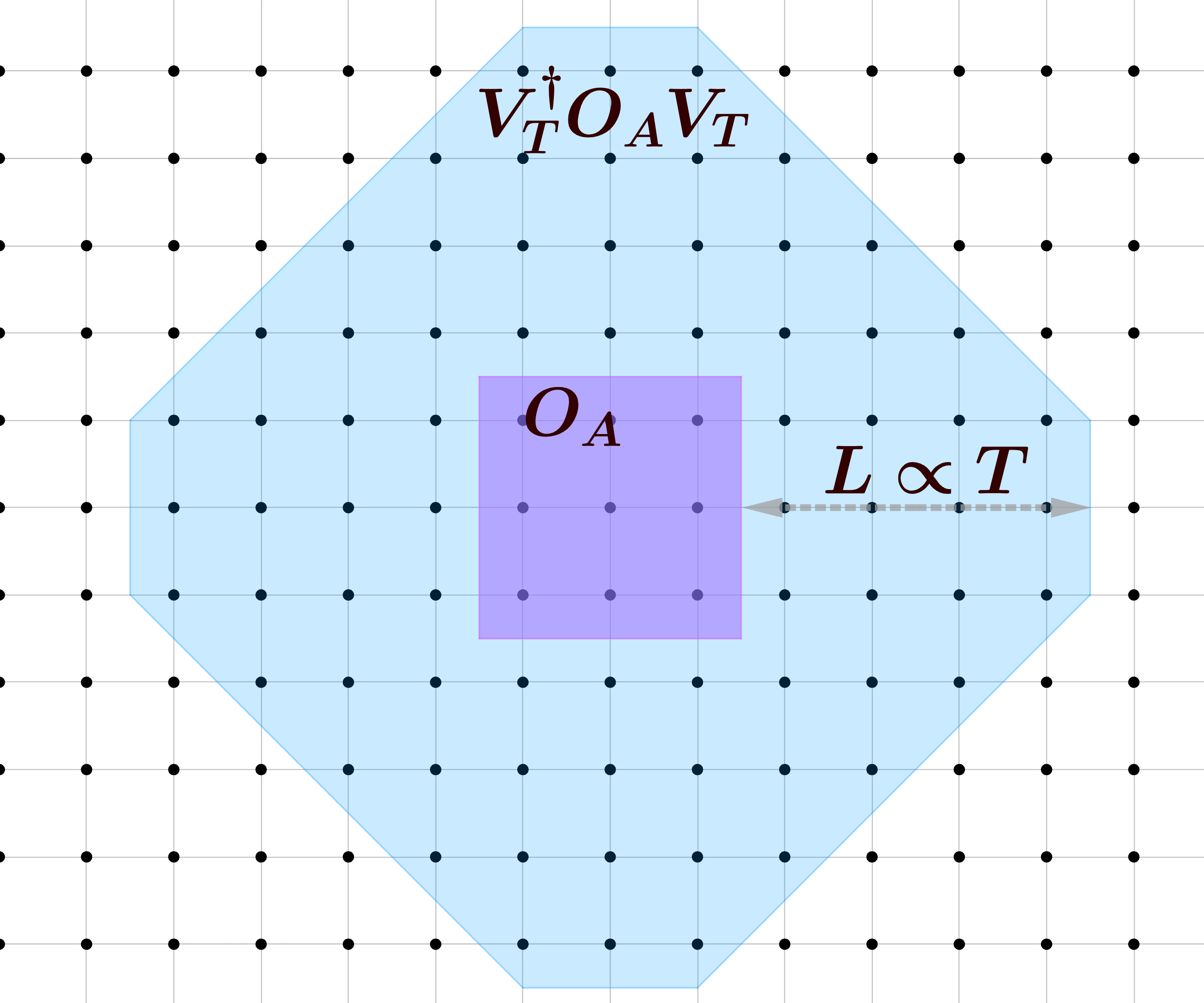
Intuitively speaking, this theorem says that, as 𝐎A\mathbf{O}_{A} is local, it remains almost local under a short-time evolution of a local Hamiltonian. Indeed, since 𝐇~A(t)\widetilde{\mathbf{H}}_{A}(t) is non-trivial only in the region AL(A)A\cup\partial_{L}(A), then 𝐕A(T)\mathbf{V}_{A}(T) also acts non-trivially only on this region. Therefore, by this theorem as it is schematically depicted in Fig. 1, 𝐔(T)𝐎A𝐔(T)\mathbf{U}^{\dagger}(T)\mathbf{O}_{A}\mathbf{U}(T) is approximated by 𝐕A(T)𝐎A𝐕A(T)\mathbf{V}^{\dagger}_{A}(T)\mathbf{O}_{A}\mathbf{V}_{A}(T) that acts only on AL(A)A\cup\partial_{L}(A).

Refer to caption
Figure 1: (Color online) Illustration of 1. Here, AA is the region on which the operator 𝐎A\mathbf{O}_{A} acts, and the larger shaded area represents L(A)\partial_{L}(A). 𝐕A(T)𝐎A𝐕A(T)\mathbf{V}^{\dagger}_{A}(T)\mathbf{O}_{A}\mathbf{V}_{A}(T) acts non-trivially on AL(A)A\cup\partial_{L}(A) and approximates 𝐔(T)𝐎A𝐔(T)\mathbf{U}^{\dagger}(T)\mathbf{O}_{A}\mathbf{U}(T), the time evolution of 𝐎A\mathbf{O}_{A} in the Heisenberg picture.

Some remarks are in line regarding this theorem. First, as the proof of this theorem given in Appendix A shows, the above Lieb-Robinson bound can easily be generalized for local Hamiltonians with kk-body interactions, by replacing the term log(4g(Δ1))\log(4g(\Delta-1)) on the right hand side of Eq. 5 with log(2kg(Δ1))\log(2kg(\Delta-1)). Second, this theorem in the case where 𝐇\mathbf{H} is time-independent is proven in [41, 37, 38]. Third, the type of time-dependent Hamiltonians (Equation 3) considered by this theorem are motivated by some quantum annealing applications in mind. Nevertheless, note that in principle any time-dependent Hamiltonian can be written in this form; simply consider the expansion of each local term of the Hamiltonian in the Pauli basis.

3 Limits on the output distribution of short-time evaluations

In this section we present our main results, namely, how the output distribution of a short-time quantum annealing algorithm is constrained. Our first main result is a generalization of the well-known Chebyshev inequality in probability theory that is a concentration of measure inequality. Our second result is an isoperimetric inequality. A similar result for low-depth circuits has been proven in [31].

In the following we assume that 𝐇(t)\mathbf{H}(t) is a time-dependent Hamiltonian defined on the vertices of a graph GG as in Eq. 3. We assume that starting with a product state

|ψ0=|s1|s2|sn,\displaystyle\ket{\psi_0}=\ket{s_1}\otimes\ket{s_2}\otimes\cdots\otimes\ket{s_n}, (6)

the system evolves under the Hamiltonian 𝐇(t)\mathbf{H}(t). Let

|ψt=𝐔(t)|ψ0,\displaystyle\ket{\psi_t}=\mathbf{U}(t)\ket{\psi_0}, (7)

where as before 𝐔(t)\mathbf{U}(t) is the associated unitary evolution. We assume that at time TT we make a measurement in the computational basis to a get a distribution p(𝐱)p(\mathbf{x}) on {0,1}n\{0,1\}^{n}.

3.1 A Chebyshev bound

Theorem 2 (Quantum Chebyshev bound).

Let 𝐇(t)\mathbf{H}(t) be a Hamiltonian on a graph with maximum degree Δ>1\Delta>1 as in Eq. 3 with ue(t)𝐡eg\|u_{e}(t)\mathbf{h}_{e}\|\leq g for any edge ee. Let

Tκ18gΔ2κ1κ1logΔlogn,\displaystyle T\leq\frac{\kappa_{1}}{8g\Delta^{\frac{2-\kappa_{1}}{\kappa_{1}}}\log\Delta}\log n, (8)

where 0<κ1<10<\kappa_{1}<1 is an arbitrary constant. Let p(𝐱)p(\mathbf{x}) be the output distribution of measuring |ψT=𝐔(T)|ψ0\ket{\psi_T}=\mathbf{U}(T)\ket{\psi_0} in the computational basis. We assume |ψ0\ket{\psi_0} to be a product state as in Eq. 6. Then for any c>0c>0 and κ1/2<κ2<1/2\kappa_{1}/2<\kappa_{2}<1/2 we have

Pr[|wH(𝐱)(n2m2)|cn12+κ2]\displaystyle\Pr\left[\left|w_{H}(\mathbf{x})-\left(\frac{n}{2}-\frac{m}{2}\right)\right|\geq cn^{\frac{1}{2}+\kappa_{2}}\right] (9)
32c2n(2κ2κ1),\displaystyle\leq\frac{3}{2c^{2}}n^{-(2\kappa_{2}-\kappa_{1})},

where wH(𝐱)w_{H}(\mathbf{x}) is the hamming weight of 𝐱{0,1}n\mathbf{x}\in\{0,1\}^{n}, i.e. number of non-zero coordinates of 𝐱\mathbf{x}, and m=iψT|𝐙i|ψTm=\sum_{i}\bra{\psi_T}\mathbf{Z}_{i}\ket{\psi_T} with 𝐙\mathbf{Z} being the Pauli-zz operator.

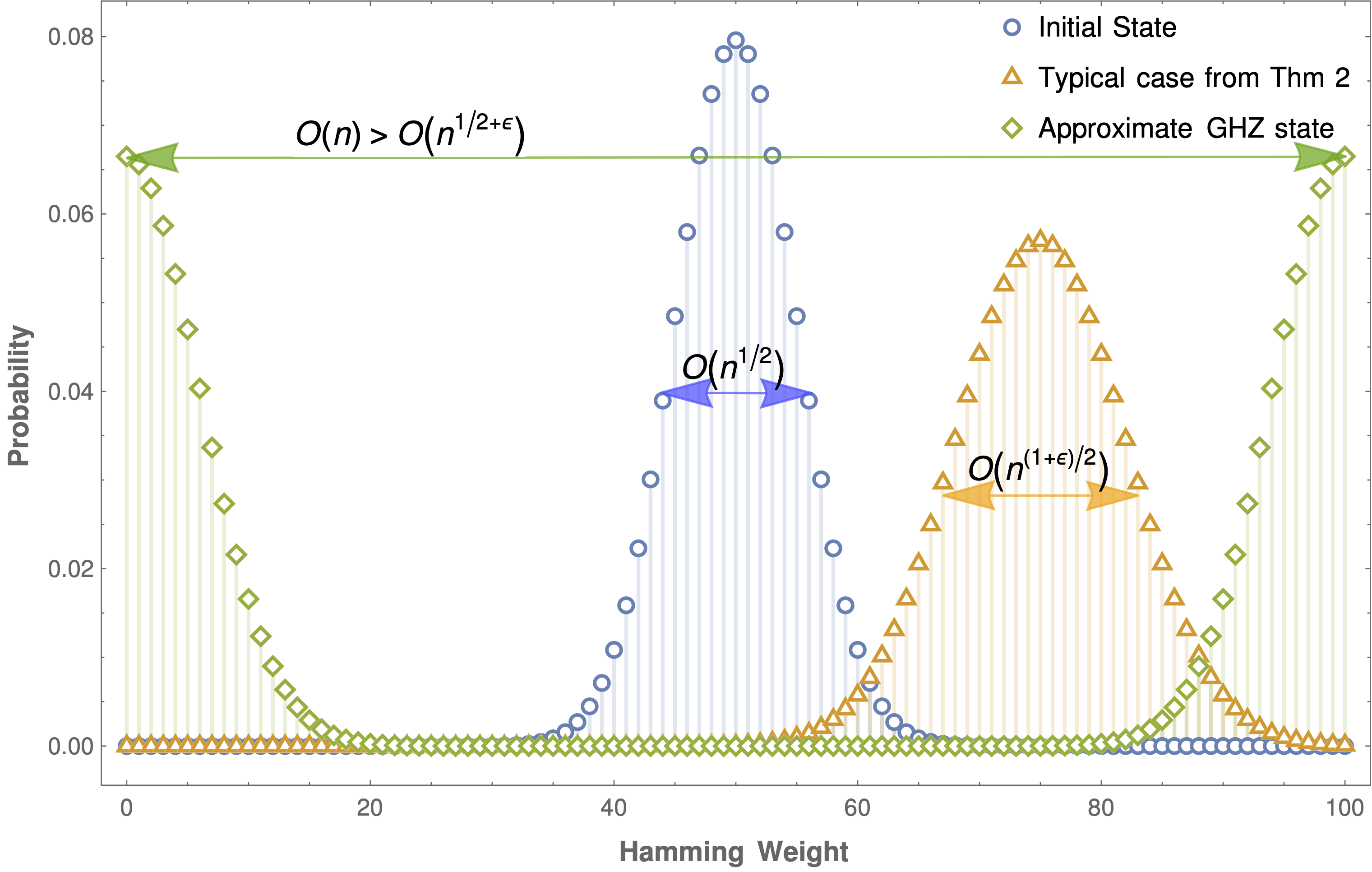
This theorem says that, when TT is bounded, with high probability the hamming weight of the measurement output is close to 12(nm)\frac{1}{2}(n-m) which is the average of wH(𝐱)w_{H}(\mathbf{x}). That is, the Hamming weight of the measurement outcome is concentrated.

The proof idea of this theorem is similar to that of the standard Chebyshev inequality; we need to bound the variance of wH(𝐱)w_{H}(\mathbf{x}). In the standard Chebyshev inequality the coordinates of 𝐱\mathbf{x} are independent while here they are correlated. Nevertheless, since TT is bounded, by the Lieb-Robinson bound (1) pairs of coordinates whose associated Hamming weights are far from each other are almost independent. This allows us to bound the variance of wH(𝐱)w_{H}(\mathbf{x}). A detailed proof of this theorem is given in Appendix B.

As a result of this theorem, as long as the initial state is a product state, no short-time annealing computation can produce the nn-qubit GHZ state 12(|00+|11)\frac{1}{\sqrt{2}}(\ket{0\cdots 0}+\ket{1\cdots 1}) in sub-logarithmic times. This is because measuring this state in the computational basis gives two far apart peaks in the hamming weight wHw_{H}, Fig. 2. We note that this statement holds for any annealing computation even with gapless Hamiltonians. Intuitively speaking, this is a result of the local nature of the Hamiltonian in Eq. 3.
Refer to caption
Figure 2: (Color online) Illustration of Theorem 2 depicting the probability distribution of the Hamming weight of three different nn-qubit states for n=100n=100. The centered distribution in the middle (blue) is the typical distribution for a product initial state (e.g., |+n\ket{+}^{\otimes n}). The distribution that is peaked just to the right (orange) represents the distribution after a short time evolution of the initial state described by 2. The distribution that has two peaks on either side of the spectrum (green) is an approximation for the GHZ state. This shows that the GHZ state cannot be generated even approximately by a short-time quantum annealing.

3.2 An isoperimetric inequality

We now prove that the output distribution of a short-time quantum annealing algorithm satisfies an isoperimetric inequality, see Figs. 3 and 4. Such a result for low-depth circuits was first proved in [31].

Theorem 3.

Let 𝐇(t)\mathbf{H}(t) be a Hamiltonian on a graph with maximum degree Δ>1\Delta>1 as in Eq. 3 with ue(t)𝐡eg\|u_{e}(t)\mathbf{h}_{e}\|\leq g for any edge ee. Let |ψ0=|s1|s2|sn\ket{\psi_0}=\ket{s_1}\otimes\ket{s_2}\otimes\cdots\otimes\ket{s_n} be an arbitrary product state and let |ψT=𝐔(T)|ψ0\ket{\psi_T}=\mathbf{U}(T)\ket{\psi_0} be the state of the system at time T>0T>0. Let p(𝐱)p(\mathbf{x}) be the distribution on {0,1}n0\{0,1\}^{n_{0}} resulting from measuring the first n0n_{0} qubits of |ψT\ket{\psi_T} in the computational basis, i.e.,

p(𝐱)\displaystyle p(\mathbf{x}) =𝐲{0,1}nn0|𝐱,𝐲|ψT|2.\displaystyle=\sum_{\mathbf{y}\in\{0,1\}^{n-n_{0}}}\absolutevalue{\braket{\vb x,\vb y}{\psi_T}}^{2}. (10)

Then for any F{0,1}n0F\subset\{0,1\}^{n_{0}} with p(F)12p(F)\leq\frac{1}{2} and any 0θ1/20\leq\theta\leq 1/2 the following results hold:

  • (i)

    Assume that

    Tκ14glog(Δ)Δ1+2κ1+κ2κ1logn0,T\leq\frac{\kappa_{1}}{4g\log(\Delta)\Delta^{\frac{1+2\kappa_{1}+\kappa_{2}}{\kappa_{1}}}}\log n_{0}\,, (11)

    for some constants κ1,κ2>0\kappa_{1},\kappa_{2}>0. Then we have

    p((F))18(2n01+κ1)2θp(F)2n0κ2.\displaystyle p\big(\partial_{\ell}(F)\big)\geq\frac{1}{8}(2n_{0}^{1+\kappa_{1}})^{-2\theta}p(F)-2n_{0}^{-\kappa_{2}}. (12)

    where

    =κ12log(Δ)log(n0)n0(12θ)(1+κ1).\ell=\frac{\kappa_{1}}{\sqrt{2}\log(\Delta)}\log(n_0)n_{0}^{\big(\frac{1}{2}-\theta\big)(1+\kappa_{1})}\,. (13)
  • (ii)

    Assume that we measure all the qubits, i.e. n0=nn_{0}=n. Moreover, assume that

    Tκ14g(Δ1)logn,T\leq\frac{\kappa_{1}}{4g(\Delta-1)}\log n\,, (14)

    and

    =κ1(1+κ2)2log(n)n\displaystyle\ell=\frac{\kappa_{1}(1+\kappa_{2})}{2}\log(n)\sqrt{n} (15)

    for some constants κ1,κ2>0\kappa_{1},\kappa_{2}>0. Then we have

    p((F))18p(F)54n(κ1(1+κ2)log(1+κ2)1).p(\partial_{\ell}(F))\geq\frac{1}{8}p(F)-\frac{5}{4}n^{-\big(\kappa_{1}(1+\kappa_{2})\log(1+\kappa_2)-1\big)}. (16)

This theorem says that, measuring in terms of the outcome probabilities of a short-time quantum annealing computation, the size of a boundary of a set is large comparing to the size of a set itself, see Fig. 3. The proof of this theorem is given in Appendix D.
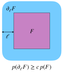
Figure 3: (Color online) A schematic presentation of the isoperimetric inequality, stating that the boundary of a region is large comparing to the region itself.
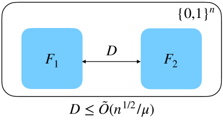
Figure 4: (Color online) 4 says that measuring in terms of the output distribution of a short-time QA algorithm, if two sets have size at least μ\mu, then their distance (ignoring some logarithmic factors) is at most n1/2/μn^{1/2}/\mu.
Theorem 4.

Let 𝐇(t)\mathbf{H}(t) be a Hamiltonian on a graph with maximum degree Δ>1\Delta>1 as in Eq. 3 with ue(t)𝐡eg\|u_{e}(t)\mathbf{h}_{e}\|\leq g for any edge ee. Let |ψ0=|s1|s2|sn\ket{\psi_0}=\ket{s_1}\otimes\ket{s_2}\otimes\cdots\otimes\ket{s_n} be an arbitrary product state and let |ψT=𝐔(T)|ψ0\ket{\psi_T}=\mathbf{U}(T)\ket{\psi_0} be the state of the system at time T>0T>0. Let p(𝐱)p(\mathbf{x}) be the distribution on {0,1}n\{0,1\}^{n} resulting from measuring qubits of |ψT\ket{\psi_T} in the computational basis. Moreover, assume that

T\displaystyle T κ14g(Δ1)logn,\displaystyle\leq\frac{\kappa_{1}}{4g(\Delta-1)}\log n,\, (17)
\displaystyle\ell =κ1(1+κ2)2log(n)n,\displaystyle=\frac{\kappa_{1}(1+\kappa_{2})}{2}\log(n)\sqrt{n},

for some constants κ1,κ2>0\kappa_{1},\kappa_{2}>0. Then for two arbitrary disjoint sets F1,F2{0,1}nF_{1},F_{2}\subset\{0,1\}^{n} with Hamming distance D=distH(F1,F2)D=\dist_{H}(F_{1},F_{2}) and μ:=min{p(F1),p(F2)}\mu:=\min\{p(F_{1}),p(F_{2})\}, we have

D\displaystyle D <16μ+10Dμn(κ1(1+κ2)log(1+κ2)1)\displaystyle<\frac{16\ell}{\mu}+\frac{10D}{\mu}n^{-\big(\kappa_{1}(1+\kappa_{2})\log(1+\kappa_2)-1\big)} (18)
16μ+10μn(κ1(1+κ2)log(1+κ2)2).\displaystyle\leq\frac{16\ell}{\mu}+\frac{10}{\mu}n^{-\big(\kappa_{1}(1+\kappa_{2})\log(1+\kappa_2)-2\big)}. (19)

The contra-positive version of this theorem says that if two far apart subsets of {0,1}n\{0,1\}^{n} have high probability under the distribution produced by the annealing algorithm, then the run-time of the annealing algorithm is necessarily long.

Here is a high level perspectice of how the proofs are laid out in the appendix. In order to prove 3, we need to bound the derivative of a certain Chebyshev polynomial of some quantum operators. Because of the approximate nature of the Lieb-Robinson bound, proving this requires an accurate mathematical analysis of the polynomials using the γ2\gamma_{2}-norm. More naive approaches would have disproportionately large errors. The proof is laid out in Appendix C. Then, by utilizing these results we prove 3 in Appendix D. 4 is basically a corollary of 3 and it is proven in Appendix E.

4 MAXCUT on Ramanujan Graphs

In this section and the following one, we present limits of short-time quantum annealing algorithms for the MaxCut problem. Here, inspired by [28] our strategy is to use the 2\mathbb{Z}_{2}-symmetry of the MaxCut Hamiltonian, and show that short-time quantum annealing algorithm cannot outperform best classical algorithms for MaxCut on Ramanujan graphs [42].

We first describe the quantum annealing algorithm for MaxCut.

Given a graph G=(V,E)G=(V,E), the MaxCut problem asks for a cut with maximum size in GG; meaning what is the maximum number of edges between vertices in V+V_{+} and VV_{-} where V+V=VV_{+}\cup V_{-}=V form a partition of vertices? Labeling vertices in V+V_{+} with +1+1 and vertices in VV_{-} with 1-1, this problem is equivalent to minimizing the energy of the following Hamiltonian:

𝐂:=12(i,j)E(𝐈𝐙i𝐙j),\mathbf{C}:=-\frac{1}{2}\sum_{(i,j)\in E}{\left(\mathbf{I}-\mathbf{Z}_{i}\mathbf{Z}_{j}\right)}, (20)

Where 𝐙i\mathbf{Z}_{i}’s are the Pauli-zz operators. Indeed, letting Cut\Cut^{*} be the maximum cut of GG we have

Cut=min|ϕϕ|𝐂|ϕ.\Cut^{*}=-\min_{\ket{\phi}}\bra{\phi}\mathbf{C}\ket{\phi}. (21)

We may use quantum annealing to find the ground state and minimum energy of 𝐂\mathbf{C}. To this end, a common choice for the driving Hamiltonian is the summation of Pauli-xx operators:

𝐁:=kV𝐗k.\mathbf{B}:=-\sum_{k\in V}\mathbf{X}_{k}. (22)

Using a control parameter u:[0,T][0,1]u:[0,T]\to[0,1] with u(0)=0u(0)=0 and u(T)=1u(T)=1, the resulting time-dependent Hamiltonian is given by

𝐇(t):=(1u(t))𝐁+u(t)𝐂\mathbf{H}(t):=\left(1-u(t)\right)\mathbf{B}+u(t)\mathbf{C} (23)

At time t=0t=0, we start with the ground state of 𝐇(0)=𝐁\mathbf{H}(0)=\mathbf{B} that is equal to

|ψ0=|+n,\displaystyle\ket{\psi_0}=\ket{+}^{\otimes n}, (24)

where n=|V|n=|V| is the number of vertices. In the following we show that if TT is bounded, then

ψT|𝐂|ψT,\bra{\psi_T}\mathbf{C}\ket{\psi_T}, (25)

is bounded away from the ground energy, i.e., Cut-\Cut^{*}, for a certain family of graphs to be defined.

For a graph G=(V,E)G=(V,E) on nn vertices, its Cheeger constant is defined by [43]:

h(G)=minSV,0<|S|n2|E(S)||S|,h(G)=\min_{S\subset V,0<\absolutevalue{S}\leq\frac{n}{2}}\frac{\absolutevalue{\partial^E(S)}}{\absolutevalue{S}}\,, (26)

where E(S)\partial^{E}(S) is the set of edges with one end in SS and one end outside of SS. Ramanujan graphs are certain families of graphs that have a large Cheeger constant; for a Δ\Delta-regular Ramanujan graph GG we have

h(G)12(Δ2Δ1).h(G)\geq\frac{1}{2}\big(\Delta-2\sqrt{\Delta-1}\big). (27)

It is known that [44, 45, 46] for any Δ3\Delta\geq 3 there exists an infinite family of Δ\Delta-regular bipartite Ramanujan graphs. We note that for such a graph, as a bipartite graph, we have

Cut=|E|=12Δn.\Cut^{*}=|E|=\frac{1}{2}\Delta n. (28)
Theorem 5.

Let GG be a Δ\Delta-regular bipartite Ramanujan graph on nn vertices. Consider the quantum annealing algorithm given by Eqs. 23 and 24. Assume that TT satisfies

Tκ14Δlogn,T\leq\frac{\kappa_{1}}{4\Delta}\log n\,, (29)

for some κ1>0\kappa_{1}>0. Then, for any 0<α<1/20<\alpha<1/2, 0<ϵ<10<\epsilon<1 and sufficiently large nn we have

ψT|𝐂|ψTCut<1α(1ϵ)+2α(1ϵ)Δ1Δ.\frac{-\bra{\psi_T}\mathbf{C}\ket{\psi_T}}{\Cut^{*}}<1-\alpha(1-\epsilon)+2\alpha(1-\epsilon)\frac{\sqrt{\Delta-1}}{\Delta}. (30)

We note that for appropriate choices of α,ϵ\alpha,\epsilon and for sufficiently large (but constant) Δ6\Delta\geq 6, the right hand side of Eq. 30 can be made smaller than 0.878560.87856. This means that the quantum annealing algorithm with TO(logn)T\leq O(\log n) does not improve on the classical algorithm of Goemans and Williamson for MaxCut [47].

As the proof of this theorem in Appendix F shows, the smallest nn for which the bound Eq. 30 holds can be explicitly estimated in terms of α,ϵ,κ1\alpha,\epsilon,\kappa_{1} and Δ\Delta.

We remark that, comparing to Eq. 14, in Eq. 29 the parameter Δ\Delta is replaced with Δ+1\Delta+1. The point is that in the MaxCut Hamiltonian Eq. 23, the number of terms acting on a vertex is Δ+1\Delta+1 due to the extra term coming from 𝐁\mathbf{B}.

5 MAXCUT on Random Bipartite Graphs

Inspired by the recent work of Farhi, Gamarnik and Gutmann [26], in this section we claim that short-time QA algorithm for MaxCut does not perform well on random bipartite graphs. The idea is that such a short-time QA algorithm does not see the whole graph, so it cannot distinguish between a bipartite random graph and an arbitrary random graph. Thus, the output cut-size of these algorithms on random bipartite graphs is bounded by the MaxCut of arbitrary random graphs.

Theorem 6.

Consider the QA algorithm using the Hamiltonian (23) with the initial state |ψ0=|+n\ket{\psi_0}=\ket{+}^{\otimes n}, and time

Tκ16log(Δ)Δ1+4/κlogn,T\leq\frac{\kappa}{16\log(\Delta)\Delta^{1+4/\kappa}}\log n\,, (31)

for some 0<κ<10<\kappa<1. Then, for any ν>0\nu>0 and sufficiently large nn, the expected cut size from applying the algorithm on a random Δ\Delta-regular bipartite graphs is at most

(Δ4+O(Δ)+2ν)n.\displaystyle\left(\frac{\Delta}{4}+O(\sqrt{\Delta})+2\nu\right)n\,. (32)

Note that, by the bound in Eq. 32, the performance of the QA algorithm on random Δ\Delta-regular bipartite graphs is not much better than outputting a random cut.

The proof of this theorem is given in Appendix G.

Farhi et al also show how the low-depth QAOA algorithm cannot outperform classical algorithms for the maximum independent set problem on random bipartite graphs [26]. Using similar arguments to what we provided in this section, that result can also be generalized to short-time QA algorithms.

6 Conclusions

Motivated by short-time quantum annealing, in this manuscript we proved limits on the output distribution of local time-dependent Hamiltonian evolutions. In particular, we showed that the distribution of the measurement outcome of a local Hamiltonian evolution is concentrated and satisfies an isoperimetric inequality if the evolution time is short. Using our framework, we generalized results about limitations of low-depth quantum circuits, to short-time QA algorithms. To this end, an essential tool that we developed, is a Lieb-Robinson bound that works for time-dependent Hamiltonians and is amenable to QA algorithms.

Our results are general in the sense that they work for the circuit model as well; they imply limitations on the output distribution of low-depth circuits with a locality structure. The point is that we can assume that the control parameters ue(t)u_{e}(t) in Eq. 3 have a so-called bang-bang form: they are either zero or take a fixed value, and for each tt the values of ue1(t),ue2(t)u_{e_{1}}(t),u_{e_{2}}(t) for intersecting edges e1,e2e_{1},e_{2} cannot both be non-zero. With such bang-bang control parameters, low-depth local circuits can be seen as special cases of short-time evolutions of local Hamiltonians for which our results hold.

The short-time condition is strictly essential for the bounds we have proven, and our results do not hold without this assumption. Indeed, there are several known examples where quantum annealing with Poly(n)\textup{Poly}(n) run-time can provide superpolynomial speedups. For example, see [48, 49, 50].

We believe that the techniques presented here can be applied to generalize other results about the limitation of low-depth circuits too, see e.g. [29, 27], for short-time QA algorithm. We leave this for future research.

References

Appendix A Proof of the Lieb-Robinson Bound

In this appendix we give a proof of 1. As mentioned before, the proof ideas are essentially the same as those of the original Lieb-Robinson bound. Here, for simplicity of presentation of the proof we first give two lemmas.

Lemma 1.

([37]) Let 𝐗=𝐗(t)\mathbf{X}=\mathbf{X}(t) and 𝐘=𝐘(t)\mathbf{Y}=\mathbf{Y}(t) be time-dependent bounded operators with 𝐗\mathbf{X} being Hermitian. Let 𝐅=𝐅(t)\mathbf{F}=\mathbf{F}(t) be given by

ddt𝐅=i[𝐗,𝐅]+𝐘.\frac{\differential}{\differential t}\mathbf{F}=i[\mathbf{X},\mathbf{F}]+\mathbf{Y}. (33)

Then we have

ddt𝐅(t)𝐘(t).\frac{\differential}{\differential t}\|\mathbf{F}(t)\|\leq\|\mathbf{Y}(t)\|. (34)
Proof.

Writing the definition of the derivative we have

ddt𝐅\displaystyle\frac{\differential}{\differential t}\|\mathbf{F}\| =limh0𝐅(t+h)𝐅(t)h\displaystyle=\lim_{h\to 0}\frac{\|\mathbf{F}(t+h)\|-\|\mathbf{F}(t)\|}{h} (35)
=limh0𝐅(t)+ih[𝐗(t),𝐅(t)]+h𝐘(t)+O(h2)𝐅(t)h\displaystyle=\lim_{h\to 0}\frac{\|\mathbf{F}(t)+ih[\mathbf{X}(t),\mathbf{F}(t)]+h\mathbf{Y}(t)\|+O(h^{2})-\|\mathbf{F}(t)\|}{h}
=limh0(I+ih𝐗)𝐅(Iih𝐗)+ih2𝐗𝐅𝐗+h𝐘𝐅h\displaystyle=\lim_{h\to 0}\frac{\|(I+ih\mathbf{X})\mathbf{F}(I-ih\mathbf{X})+ih^{2}\mathbf{X}\mathbf{F}\mathbf{X}+h\mathbf{Y}\|-\|\mathbf{F}\|}{h}
=limh0eih𝐗𝐅eih𝐗+ih2𝐗𝐅𝐗+h𝐘+O(h2)𝐅h\displaystyle=\lim_{h\to 0}\frac{\|\e^{ih\mathbf{X}}\mathbf{F}\e^{-ih\mathbf{X}}+ih^{2}\mathbf{X}\mathbf{F}\mathbf{X}+h\mathbf{Y}\|+O(h^{2})-\|\mathbf{F}\|}{h}
limh0eih𝐗𝐅eih𝐗𝐅h+h𝐗𝐅𝐗+𝐘\displaystyle\leq\lim_{h\to 0}\frac{\|\e^{ih\mathbf{X}}\mathbf{F}\e^{-ih\mathbf{X}}\|-\|\mathbf{F}\|}{h}+h\|\mathbf{X}\mathbf{F}\mathbf{X}\|+\|\mathbf{Y}\|
=𝐘,\displaystyle=\|\mathbf{Y}\|\,,

where in the fourth line we use e±ih𝐗=I±ih𝐗+O(h2)\e^{\pm ih\mathbf{X}}=I\pm ih\mathbf{X}+O(h^{2}), and in the last line we use the fact that 𝐗\mathbf{X} is Hermitian and e±ih𝐗e^{\pm ih\mathbf{X}} is unitary. ∎

Here is our second building block of the proof.

Lemma 2.

Using the notation of 1 and assuming that L>1L>1 we have

𝐔(t)𝐎𝐔(t)𝐕(t)𝐎𝐕(t)2𝐎AeA0t|ue(τ)|𝐔(τ)𝐡e𝐔(τ)𝐕(τ)𝐡e𝐕(τ)dτ,\big\|\mathbf{U}(t)^{\dagger}\mathbf{O}\mathbf{U}(t)-\mathbf{V}(t)^{\dagger}\mathbf{O}\mathbf{V}(t)\big\|\leq 2\|\mathbf{O}_{A}\|\sum_{e\sim A}\int_{0}^{t}|u_{e}(\tau)|\cdot\big\|\mathbf{U}^{\dagger}(\tau)\mathbf{h}_{e}\mathbf{U}(\tau)-\mathbf{V}(\tau)^{\dagger}\mathbf{h}_{e}\mathbf{V}(\tau)\big\|\differential\tau\,, (36)

where 𝐇~A(t):=eAL(A)ue(t)𝐡e\mathbf{\widetilde{H}}_{A}(t):=\sum_{e\subseteq A\cup\partial_{L}(A)}u_{e}(t)\mathbf{h}_{e} is the Hamiltonian consisting of terms in the region AL(A)A\cup\partial_{L}(A), and 𝐕(t)\mathbf{V}(t) is the unitary evolution associated to 𝐇~A(t)\mathbf{\widetilde{H}}_{A}(t). Also, by eAe\sim A we mean ee intersects AA. Moreover, if A=e0A=e_{0} for some edge e0e_{0} and 𝐎A=𝐡e0\mathbf{O}_{A}=\mathbf{h}_{e_{0}}, then the sum in Eq. 36 can be further restricted to ee0e\neq e_{0}.

Proof.

Let

𝐅(t):=𝐔(t)𝐎𝐔(t)𝐕(t)𝐎𝐕(t).\mathbf{F}(t):=\mathbf{U}(t)^{\dagger}\mathbf{O}\mathbf{U}(t)-\mathbf{V}(t)^{\dagger}\mathbf{O}\mathbf{V}(t). (37)

Then from Schrodinger’s equation we have

ddt𝐅(t)\displaystyle\frac{\differential}{\differential t}\mathbf{F}(t) =i𝐔(t)[𝐇(t),𝐎]𝐔(t)i𝐕(t)[𝐇~(t),𝐎]𝐕(t)\displaystyle=i\mathbf{U}(t)^{\dagger}\big[\mathbf{H}(t),\mathbf{O}\big]\mathbf{U}(t)-i\mathbf{V}(t)^{\dagger}\big[\mathbf{\widetilde{H}}(t),\mathbf{O}\big]\mathbf{V}(t) (38)
=eAi𝐔(t)[𝐡e(t),𝐎]𝐔(t)i𝐕(t)[𝐡e(t),𝐎]𝐕(t)\displaystyle=\sum_{e\sim A}i\mathbf{U}(t)^{\dagger}\big[\mathbf{h}_{e}(t),\mathbf{O}\big]\mathbf{U}(t)-i\mathbf{V}(t)^{\dagger}\big[\mathbf{h}_{e}(t),\mathbf{O}\big]\mathbf{V}(t)
=eAi[𝐔(t)𝐡e(t)𝐔(t),𝐔(t)𝐎𝐔(t)]i[𝐕(t)𝐡e(t)𝐕(t),𝐕(t)𝐎𝐕(t)]\displaystyle=\sum_{e\sim A}i\big[\mathbf{U}(t)^{\dagger}\mathbf{h}_{e}(t)\mathbf{U}(t),\mathbf{U}(t)^{\dagger}\mathbf{O}\mathbf{U}(t)^{\dagger}\big]-i\big[\mathbf{V}(t)^{\dagger}{\mathbf{h}}_{e}(t)\mathbf{V}(t),\mathbf{V}(t)^{\dagger}\mathbf{O}\mathbf{V}(t)\big]
=eAi[𝐔(t)𝐡e(t)𝐔(t),𝐅(t)+𝐕(t)𝐎𝐕(t)]i[𝐕(t)𝐡e(t)𝐕(t),𝐕(t)𝐎𝐕(t)]\displaystyle=\sum_{e\sim A}i\big[\mathbf{U}(t)^{\dagger}\mathbf{h}_{e}(t)\mathbf{U}(t),\mathbf{F}(t)+\mathbf{V}(t)^{\dagger}\mathbf{O}\mathbf{V}(t)^{\dagger}\big]-i\big[\mathbf{V}(t)^{\dagger}{\mathbf{h}}_{e}(t)\mathbf{V}(t),\mathbf{V}(t)^{\dagger}\mathbf{O}\mathbf{V}(t)\big]
=i[eA𝐔(t)𝐡e(t)𝐔(t),𝐅(t)]+ieA[𝐔(t)𝐡e(t)𝐔(t)𝐕(t)𝐡e(t)𝐕(t),𝐕(t)𝐎𝐕(t)].\displaystyle=i\Big[\sum_{e\sim A}\mathbf{U}(t)^{\dagger}\mathbf{h}_{e}(t)\mathbf{U}(t),\mathbf{F}(t)\Big]+i\sum_{e\sim A}\big[\mathbf{U}(t)^{\dagger}{\mathbf{h}}_{e}(t)\mathbf{U}(t)-\mathbf{V}(t)^{\dagger}{\mathbf{h}}_{e}(t)\mathbf{V}(t),\mathbf{V}(t)^{\dagger}\mathbf{O}\mathbf{V}(t)\big]\,.

Therefore, using 𝐅(0)=0\mathbf{F}(0)=0 and 1 we can bound

𝐅(t)\displaystyle\|\mathbf{F}(t)\| =0tddτ𝐅(τ)dτ\displaystyle=\left\|\int_{0}^{t}\frac{\differential}{\differential\tau}\mathbf{F}(\tau)\differential\tau\right\| (39)
0tddτ𝐅(τ)dτ\displaystyle\leq\int_{0}^{t}\Big\|\frac{\differential}{\differential\tau}\mathbf{F}(\tau)\Big\|\differential\tau
0teA[𝐔(τ)𝐡e(τ)𝐔(τ)𝐕(τ)𝐡e(τ)𝐕(τ),𝐕(τ)𝐎𝐕(τ)]dτ\displaystyle\leq\int_{0}^{t}\sum_{e\sim A}\big\|\big[\mathbf{U}(\tau)^{\dagger}{\mathbf{h}}_{e}(\tau)\mathbf{U}(\tau)-\mathbf{V}(\tau)^{\dagger}{\mathbf{h}}_{e}(\tau)\mathbf{V}(\tau),\mathbf{V}(\tau)^{\dagger}\mathbf{O}\mathbf{V}(\tau)\big]\big\|\differential\tau
2𝐎eA0t|ue(τ)|𝐔(τ)𝐡e𝐔(τ)𝐕(τ)𝐡e𝐕(τ)dτ,\displaystyle\leq 2\|\mathbf{O}\|\sum_{e\sim A}\int_{0}^{t}|u_{e}(\tau)|\cdot\big\|\mathbf{U}(\tau)^{\dagger}{\mathbf{h}}_{e}\mathbf{U}(\tau)-\mathbf{V}(\tau)^{\dagger}{\mathbf{h}}_{e}\mathbf{V}(\tau)\big\|\differential\tau\,,

where we use [𝐗,𝐘]2𝐗𝐘\|[\mathbf{X},\mathbf{Y}]\|\leq 2\|\mathbf{X}\|\|\mathbf{Y}\| in the last line. Note that if 𝐎A=𝐡e0\mathbf{O}_{A}=\mathbf{h}_{e_{0}}, in the second line of Eq. 38 and thereafter, we can further restrict the sum to ee0e\neq e_{0}.

We can now give the proof of 1. As before, let 𝐅(t):=𝐔(t)𝐎𝐔(t)𝐕(t)𝐎𝐕(t)\mathbf{F}(t):=\mathbf{U}(t)^{\dagger}\mathbf{O}\mathbf{U}(t)-\mathbf{V}(t)^{\dagger}\mathbf{O}\mathbf{V}(t). By 2 we have

𝐅(T)2𝐎e1A0T|ue1(t1)|𝐔(t1)𝐡e1𝐔(t1)𝐕(t1)𝐡e1𝐕(t1)dt1.\|\mathbf{F}(T)\|\leq 2\|\mathbf{O}\|\sum_{e_{1}\sim A}\int_{0}^{T}|u_{e_{1}}(t_{1})|\cdot\big\|\mathbf{U}(t_{1})^{\dagger}{\mathbf{h}}_{e_{1}}\mathbf{U}(t_{1})-\mathbf{V}(t_{1})^{\dagger}{\mathbf{h}}_{e_{1}}\mathbf{V}(t_{1})\big\|\differential t_{1}\,. (40)

Assuming that L>2L>2, we can apply 2 on each of the terms in the above sum, in which A=e1A=e_{1} and 𝐎A\mathbf{O}_{A} is replaced by 𝐡e1\mathbf{h}_{e_{1}}. Therefore,

𝐅(T)\displaystyle\|\mathbf{F}(T)\| 2𝐎Ae1A0T2ue1(t)𝐡e10t1e2e1e2e1|ue2(t2)|𝐔(t2)𝐡e2𝐔(t2)𝐕(t2)𝐡e2𝐕(t2)dt2dt1\displaystyle\leq 2\|\mathbf{O}_{A}\|\sum_{e_{1}\sim A}\int_{0}^{T}2\|u_{e_{1}}(t)\mathbf{h}_{e_{1}}\|\int_{0}^{t_{1}}\sum_{\stackrel{{\scriptstyle e_{2}\sim e_{1}}}{{e_{2}\neq e_{1}}}}|u_{e_{2}}(t_{2})|\cdot\|\mathbf{U}(t_{2})^{\dagger}\mathbf{h}_{e_{2}}\mathbf{U}(t_{2})-\mathbf{V}(t_{2})^{\dagger}\mathbf{h}_{e_{2}}\mathbf{V}(t_{2})\|\differential t_{2}\differential t_{1} (41)
2𝐎A 2ge1Ae2e1e2e10T0t1|ue2(t2)|𝐔(t2)𝐡e2𝐔(t2)𝐕(t2)𝐡e2𝐕(t2)dt2dt1.\displaystyle\leq 2\|\mathbf{O}_{A}\|\,2g\sum_{e_{1}\sim A}\sum_{\stackrel{{\scriptstyle e_{2}\sim e_{1}}}{{e_{2}\neq e_{1}}}}\int_{0}^{T}\int_{0}^{t_{1}}|u_{e_{2}}(t_{2})|\cdot\|\mathbf{U}(t_{2})^{\dagger}\mathbf{h}_{e_{2}}\mathbf{U}(t_{2})-\mathbf{V}(t_{2})^{\dagger}\mathbf{h}_{e_{2}}\mathbf{V}(t_{2})\|\differential t_{2}\differential t_{1}\,.

We can repeat the same process for LL times to obtain

𝐅(T)2𝐎A(2g)L1\displaystyle\frac{\|\mathbf{F}(T)\|}{2\|\mathbf{O}_{A}\|(2g)^{L-1}} (42)
 walk starting at A(e1,e2,,eL):0T0t10tL1|ueL(tL)|𝐔(tL)𝐡eL𝐔(tL)𝐕(tL)𝐡e2𝐕(tL)dtLdt2dt1\displaystyle\leq\sum_{\stackrel{{\scriptstyle(e_{1},e_{2},\dots,e_{L}):}}{{\text{ walk starting at }A}}}\int_{0}^{T}\int_{0}^{t_{1}}\dots\int_{0}^{t_{L-1}}|u_{e_{L}}(t_{L})|\cdot\|\mathbf{U}(t_{L})^{\dagger}\mathbf{h}_{e_{L}}\mathbf{U}(t_{L})-\mathbf{V}(t_{L})^{\dagger}\mathbf{h}_{e_{2}}\mathbf{V}(t_{L})\|\differential t_{L}\dots\differential t_{2}\differential t_{1}
 walk starting at A(e1,e2,,eL):0T0t10tL12gdtLdt2dt1\displaystyle\leq\sum_{\stackrel{{\scriptstyle(e_{1},e_{2},\dots,e_{L}):}}{{\text{ walk starting at }A}}}\int_{0}^{T}\int_{0}^{t_{1}}\dots\int_{0}^{t_{L-1}}2g\penalty\ \differential t_{L}\dots\differential t_{2}\differential t_{1}
=2gTLL!NL,\displaystyle=2g\frac{T^{L}}{L!}N_{L}\,,

where NLN_{L} denotes the number of walks of length LL starting at AA, i.e., NLN_{L} is the number of sequences of edges (e1,,eL)(e_{1},\dots,e_{L}) such that e1Ae_{1}\sim A, eiei+1e_{i}\sim e_{i+1} and eiei+1e_{i}\neq e_{i+1} for i=1,,L1i=1,\dots,L-1. We note that as the maximum degree of the graph GG is Δ\Delta, the number of choices for e1e_{1} is at most Δ|A|2(Δ1)|A|\Delta|A|\leq 2(\Delta-1)|A|. Moreover, the number of choices for ei+1e_{i+1} given eie_{i} is at most 2(Δ1)2(\Delta-1). Thus NL(2(Δ1))L|A|N_{L}\leq(2(\Delta-1))^{L}|A|. Therefore, using the Stirling’s approximation we have

𝐅(T)\displaystyle\|\mathbf{F}(T)\| 2|A|𝐎A(4g(Δ1)T)LL!\displaystyle\leq 2|A|\penalty\ \|\mathbf{O}_{A}\|\frac{\big(4g(\Delta-1)T\big)^{L}}{L!} (43)
2|A|𝐎A(4g(Δ1)T)L12πeLlogL+L12logL\displaystyle\leq 2|A|\cdot\|\mathbf{O}_{A}\|\big(4g(\Delta-1)T\big)^{L}\frac{1}{\sqrt{2\pi}}\e^{-L\log L+L-\frac{1}{2}\log L}
2π|A|𝐎AeL(logLlogTlog((4g(Δ1))))12logL.\displaystyle\leq\sqrt{\frac{2}{\pi}}|A|\cdot\|\mathbf{O}_{A}\|\e^{-L\big(\log L-\log T-\log{(4g(\Delta-1))}\big)-\frac{1}{2}\log L}\,.

Appendix B Proof of 2

Let 𝜻=i𝐙i{\bf\it\zeta}=\sum_{i}\mathbf{Z}_{i} and use Markov’s inequality to obtain

Pr[|wH(𝐱)(n2m2)|cn12+κ2]\displaystyle\text{Pr}\left[\left|w_{H}(\mathbf{x})-\left(\frac{n}{2}-\frac{m}{2}\right)\right|\geq cn^{\frac{1}{2}+\kappa_{2}}\right] =Pr[|𝐱|𝜻|𝐱m|2cn12+κ2]\displaystyle=\text{Pr}\left[\left|\bra{\vb x}{\bf\it\zeta}\ket{\vb x}-m\right|\geq 2cn^{\frac{1}{2}+\kappa_{2}}\right] (44)
1(2cn12+κ2)2𝔼[(𝐱|𝜻|𝐱m)2].\displaystyle\leq\frac{1}{\left(2cn^{\frac{1}{2}+\kappa_{2}}\right)^{2}}\mathbb{E}\left[\big(\bra{\vb x}{\bf\it\zeta}\ket{\vb x}-m\big)^{2}\right]\,. (45)

Thus to prove the theorem it suffices to bound 𝔼[(𝐱|𝜻|𝐱m)2]\mathbb{E}\big[\big(\bra{\vb x}{\bf\it\zeta}\ket{\vb x}-m\big)^{2}\big].

Let mi=ψT|𝐙i|ψTm_{i}=\bra{\psi_T}\mathbf{Z}_{i}\ket{\psi_T}. Then we have

𝔼[(𝐱|𝜻|𝐱m)2]\displaystyle\mathbb{E}\left[\left(\bra{\vb x}{\bf\it\zeta}\ket{\vb x}-m\right)^{2}\right] (46)
=𝔼[(i𝐱|𝐙i|𝐱mi)2]\displaystyle=\mathbb{E}\left[\left(\sum_{i}\bra{\vb x}\mathbf{Z}_{i}\ket{\vb x}-m_{i}\right)^{2}\right]
=i,j𝔼[(𝐱|𝐙i|𝐱mi)(𝐱|𝐙j|𝐱mj)]\displaystyle=\sum_{i,j}\mathbb{E}\big[\big(\bra{\vb x}\mathbf{Z}_{i}\ket{\vb x}-m_{i}\big)\cdot\big(\bra{\vb x}\mathbf{Z}_{j}\ket{\vb x}-m_{j}\big)\big]
=i,jψT|(𝐙imi)(𝐙jmj)|ψT\displaystyle=\sum_{i,j}\bra{\psi_T}(\mathbf{Z}_{i}-m_{i})(\mathbf{Z}_{j}-m_{j})\ket{\psi_T}
=i,jdistG(i,j)2LψT|(𝐙imi)(𝐙jmj)|ψT+i,jdistG(i,j)>2LψT|(𝐙imi)(𝐙jmj)|ψT,\displaystyle=\sum_{\begin{subarray}{c}i,j\\ \dist_{G}(i,j)\leq 2L\end{subarray}}\bra{\psi_T}(\mathbf{Z}_{i}-m_{i})(\mathbf{Z}_{j}-m_{j})\ket{\psi_T}+\sum_{\begin{subarray}{c}i,j\\ \dist_{G}(i,j)>2L\end{subarray}}\bra{\psi_T}(\mathbf{Z}_{i}-m_{i})(\mathbf{Z}_{j}-m_{j})\ket{\psi_T}\,,

where in the third line we use the fact that 𝐙i\mathbf{Z}_{i} is diagonal in the computational basis, distG(i,j)\dist_{G}(i,j) denotes the distance of vertices i,ji,j on the graph GG, and LL is given by

L=κ12logΔlogn4gΔ2κ1κ1T.\displaystyle L=\frac{\kappa_{1}}{2\log\Delta}\log n\geq 4g\Delta^{\frac{2-\kappa_{1}}{\kappa_{1}}}T. (47)

We analyze terms in the above sum separately. If distG(i,j)2L\dist_{G}(i,j)\leq 2L, then by the Cauchy-Schwarz inequality we have

ψT|(𝐙imi)(𝐙jmj)|ψT\displaystyle\bra{\psi_T}\left(\mathbf{Z}_{i}-m_{i}\right)\left(\mathbf{Z}_{j}-m_{j}\right)\ket{\psi_T} ψT|(𝐙imi)2|ψTψT|(𝐙jmj)2|ψT\displaystyle\leq\sqrt{\bra{\psi_T}\left(\mathbf{Z}_{i}-m_{i}\right)^{2}\ket{\psi_T}\cdot\bra{\psi_T}\left(\mathbf{Z}_{j}-m_{j}\right)^{2}\ket{\psi_T}} (48)
=(1mi2)(1mj2)\displaystyle=\sqrt{(1-m_{i}^{2})(1-m_{j}^{2})} (49)
1.\displaystyle\leq 1\,. (50)

Next, by the Lieb-Robinson bound (Theorem 1), for any ii there is an operator 𝐙~i\mathbf{\tilde{Z}}_{i} that acts only on L({i})\partial_{L}(\{i\}) and

𝐔(T)(𝐙imi)𝐔(T)𝐙~ieL(logLlogTlog(4gΔ))eL(21κ1κ1logΔ)=n(1κ1),\|\mathbf{U}(T)^{\dagger}(\mathbf{Z}_{i}-m_{i})\mathbf{U}(T)-\mathbf{\tilde{Z}}_{i}\|\leq\e^{-L\big(\log L-\log T-\log{4g\Delta}\big)}\leq\e^{-L\Big(2\frac{1-\kappa_{1}}{\kappa_{1}}\log\Delta\Big)}=n^{-(1-\kappa_{1})}\,, (51)

where the second inequality follows from (47). Therefore, letting 𝚼i=𝐔(T)(𝐙imi)𝐔(T)𝐙~i\mathbf{\Upsilon}_{i}=\mathbf{U}(T)^{\dagger}(\mathbf{Z}_{i}-m_{i})\mathbf{U}(T)-\mathbf{\tilde{Z}}_{i}, if distG(i,j)>2L\dist_{G}(i,j)>2L we have

ψT|(𝐙imi)(𝐙jmj)|ψT\displaystyle\bra{\psi_T}\left(\mathbf{Z}_{i}-m_{i}\right)\left(\mathbf{Z}_{j}-m_{j}\right)\ket{\psi_T} (52)
=ψ0|𝐔(T)(𝐙imi)(𝐙jmj)𝐔(T)|ψ0\displaystyle=\bra{\psi_0}\mathbf{U}(T)^{\dagger}\left(\mathbf{Z}_{i}-m_{i}\right)\left(\mathbf{Z}_{j}-m_{j}\right)\mathbf{U}(T)\ket{\psi_0}
=ψ0|(𝐙~i+𝚼i)(𝐙~j+𝚼j)|ψ0\displaystyle=\bra{\psi_0}\left(\tilde{\mathbf{Z}}_{i}+\mathbf{\Upsilon}_{i}\right)\left(\tilde{\mathbf{Z}}_{j}+\mathbf{\Upsilon}_{j}\right)\ket{\psi_0}
=ψ0|𝐙~i𝐙~j|ψ0+ψ0|𝚼i𝐙~j|ψ0+ψ0|𝐙~i𝚼j|ψ0+ψ0|𝚼i𝚼j|ψ0\displaystyle=\bra{\psi_0}\tilde{\mathbf{Z}}_{i}\tilde{\mathbf{Z}}_{j}\ket{\psi_0}+\bra{\psi_0}\mathbf{\Upsilon}_{i}\tilde{\mathbf{Z}}_{j}\ket{\psi_0}+\bra{\psi_0}\tilde{\mathbf{Z}}_{i}\mathbf{\Upsilon}_{j}\ket{\psi_0}+\bra{\psi_0}\mathbf{\Upsilon}_{i}\mathbf{\Upsilon}_{j}\ket{\psi_0}
=ψ0|𝐙~i|ψ0ψ0|𝐙~j|ψ0+ψ0|𝚼i𝐙~j|ψ0+ψ0|𝐙~i𝚼j|ψ0+ψ0|𝚼i𝚼j|ψ0,\displaystyle=\bra{\psi_0}\tilde{\mathbf{Z}}_{i}\ket{\psi_0}\bra{\psi_0}\tilde{\mathbf{Z}}_{j}\ket{\psi_0}+\bra{\psi_0}\mathbf{\Upsilon}_{i}\tilde{\mathbf{Z}}_{j}\ket{\psi_0}+\bra{\psi_0}\tilde{\mathbf{Z}}_{i}\mathbf{\Upsilon}_{j}\ket{\psi_0}+\bra{\psi_0}\mathbf{\Upsilon}_{i}\mathbf{\Upsilon}_{j}\ket{\psi_0}\,,

where in the last line we use the facts that |ψ0\ket{\psi_0} is a product state and that the supports of 𝐙~i,𝐙~j\tilde{\mathbf{Z}}_{i},\tilde{\mathbf{Z}}_{j} do not intersect. Now we have

|ψ0|𝐙~i|ψ0|\displaystyle|\bra{\psi_0}\tilde{\mathbf{Z}}_{i}\ket{\psi_0}| =|ψT|(𝐙imi)|ψTψ0|𝚼i|ψ0|\displaystyle=|\bra{\psi_T}({\mathbf{Z}}_{i}-m_{i})\ket{\psi_T}-\bra{\psi_0}\mathbf{\Upsilon}_{i}\ket{\psi_0}| (53)
=|ψ0|𝚼i|ψ0|\displaystyle=|\bra{\psi_0}\mathbf{\Upsilon}_{i}\ket{\psi_0}| (54)
𝚼i\displaystyle\leq\|\mathbf{\Upsilon}_{i}\| (55)
n(1κ1).\displaystyle\leq n^{-(1-\kappa_{1})}. (56)

Using this, and similar inequalities, we find that

ψT|(𝐙imi)(𝐙jmj)|ψT2(n(1κ1))2+2n(1κ1)4n(1κ1).\displaystyle\bra{\psi_T}\left(\mathbf{Z}_{i}-m_{i}\right)\left(\mathbf{Z}_{j}-m_{j}\right)\ket{\psi_T}\leq 2\left(n^{-(1-\kappa_{1})}\right)^{2}+2n^{-(1-\kappa_{1})}\leq 4n^{-(1-\kappa_{1})}. (57)

Putting these together yields

𝔼[(𝐱|𝜻|𝐱m)2]\displaystyle\mathbb{E}\left[\left(\bra{\vb x}{\bf\it\zeta}\ket{\vb x}-m\right)^{2}\right] i,jdistG(i,j)2L1+i,jdistG(i,j)>2L4n(1κ1)\displaystyle\leq\sum_{\begin{subarray}{c}i,j\\ \dist_{G}(i,j)\leq 2L\end{subarray}}1+\sum_{\begin{subarray}{c}i,j\\ \dist_{G}(i,j)>2L\end{subarray}}4n^{-(1-\kappa_{1})} (58)
2nΔ2L+n2(4n(1κ1))\displaystyle\leq 2n\Delta^{2L}+n^{2}(4n^{-(1-\kappa_{1})}) (59)
=6n1+κ1,\displaystyle=6n^{1+\kappa_{1}}, (60)

where in the second line we use

1+Δ(1+(Δ1)+(Δ1)2+(Δ1)2L1)2Δ2L.\displaystyle 1+\Delta\Big(1+(\Delta-1)+(\Delta-1)^{2}+\cdots(\Delta-1)^{2L-1}\Big)\leq 2\Delta^{2L}. (61)

Using this in (45) the desired inequality follows.

Appendix C Derivative of a matrix function

In this appendix we compute a bound on the derivative of a certain polynomial function of matrices. This bound is an important ingredient in the proof of 3. Indeed, in the proof, applying the Lieb-Robinson bound, a desired operator is approximated by a local one. Then, a polynomial function is applied on this operator, and the blow-up of the error of the Lieb-Robinson approximation induced by this polynomial should be estimated. We note that a naive approach to estimate this error is ineffective since the degree of this polynomial is large and some of its coefficients are exponentially large. Therefore, we need a more careful analysis of this error which itself demands a more careful analysis of the derivative of that polynomial as a map on the space of matrices.

We first need to fix some notations. Given two matrices 𝐀\mathbf{A} and 𝐁\mathbf{B} of the same dimensions, we denote their entry-wise product by 𝐀𝐁\mathbf{A}\circ\mathbf{B}. In other words, 𝐀𝐁\mathbf{A}\circ\mathbf{B} is a matrix whose (i,j)(i,j)-th entry equals the product of (i,j)(i,j)-th entries of 𝐀\mathbf{A} and 𝐁\mathbf{B}, i.e., (𝐀𝐁)ij=𝐀ij𝐁ij(\mathbf{A}\circ\mathbf{B})_{ij}=\mathbf{A}_{ij}\cdot\mathbf{B}_{ij}. The matrix 𝐀𝐁\mathbf{A}\circ\mathbf{B} is called the Schur or Hadamard product of 𝐀\mathbf{A} and 𝐁\mathbf{B}.

For a continuously differentiable function f:(a,b)f:(a,b)\to\mathbb{R} and a sequence 𝝀=(λ1,,λd)\boldsymbol{\lambda}=(\lambda_{1},\dots,\lambda_{d}) of numbers in (a,b)(a,b) we let 𝒟f,𝝀\mathcal{D}_{f,\boldsymbol{\lambda}} be the d×dd\times d matrix whose (i,j)(i,j)-th entry equals

(𝒟f,𝝀)ij={f(λi)f(λj)λiλjλiλj,f(λi)λi=λj,\displaystyle\big(\mathcal{D}_{f,\boldsymbol{\lambda}}\big)_{ij}=\begin{cases}\frac{f(\lambda_{i})-f(\lambda_{j})}{\lambda_{i}-\lambda_{j}}&\quad\lambda_{i}\neq\lambda_{j},\\ f^{\prime}(\lambda_{i})&\quad\lambda_{i}=\lambda_{j},\end{cases} (62)

where f(λi)f^{\prime}(\lambda_{i}) is the derivative of ff at λi\lambda_{i}. For a diagonal matrix 𝚲=diag(𝝀)\mathbf{\Lambda}=\text{diag}(\boldsymbol{\lambda}) with diagonal elements in 𝝀=(λ1,,λd)\boldsymbol{\lambda}=(\lambda_{1},\dots,\lambda_{d}) we let

𝒟f,𝚲:=𝒟f,𝝀.\displaystyle\mathcal{D}_{f,\mathbf{\Lambda}}:=\mathcal{D}_{f,\boldsymbol{\lambda}}. (63)

Also, for a self-adjoint matrix 𝐀\mathbf{A}, that can be diagonalized as 𝐀=𝐔𝚲𝐔\mathbf{A}=\mathbf{U}\mathbf{\Lambda}\mathbf{U}^{\dagger} where 𝐔\mathbf{U} is unitary and 𝚲=diag(𝝀)\mathbf{\Lambda}=\text{diag}(\boldsymbol{\lambda}) is a diagonal matrix containing eigenvalues of 𝐀\mathbf{A}, we let

𝒟f,𝐀=𝐔𝒟f,𝚲𝐔.\displaystyle\mathcal{D}_{f,\mathbf{A}}=\mathbf{U}\mathcal{D}_{f,\mathbf{\Lambda}}\mathbf{U}^{\dagger}. (64)
Lemma 3.

[51, pp. 124] Let 𝐀,𝐄\mathbf{A},\mathbf{E} be two Hermitian matrices and ff be a real continuously differentiable function on an interval containing the eigenvalues of 𝐀+t𝐄\mathbf{A}+t\mathbf{E} for all t(1,1)t\in(-1,1). Then we have

ddtf(𝐀+t𝐄)|t=0=𝒟f,𝐀𝐄.\derivative{t}f\left(\mathbf{A}+t\mathbf{E}\right)\Big|_{t=0}=\mathcal{D}_{f,\mathbf{A}}\circ\mathbf{E}\,. (65)

By this lemma, to bound the derivative of a matrix function as above, we need to bound the norm of the Schur product as a super-operator on the space of matrices. This super-operator norm is given by the so called γ2\gamma_{2}-norm.

Lemma 4.

[52, pp. 79] For a d×dd\times d matrix 𝐌\mathbf{M} let

γ2(𝐌):=infmax{|vi2: 1id}{|wj2: 1jd},\displaystyle\gamma_{2}(\mathbf{M}):=\inf\,\max\{\|\ket{v_i}\|^{2}:\,1\leq i\leq d\}\cup\{\|\ket{w_j}\|^{2}:\,1\leq j\leq d\}, (66)

where the infimum is taken over all vectors |vi,|wj\ket{v_i},\ket{w_j} satisfying 𝐌ij=vi|wj\mathbf{M}_{ij}=\langle v_{i}\ket{w_j} for all i,ji,j. Then for any d×dd\times d matrix 𝐄\mathbf{E} we have

𝐌𝐄γ2(𝐌)𝐄.\displaystyle\|\mathbf{M}\circ\mathbf{E}\|\leq\gamma_{2}(\mathbf{M})\|\mathbf{E}\|. (67)

It is not hard to verify that γ2\gamma_{2}-norm as defined in Eq. 66 satisfies the triangle inequality and is a norm. We also note that if 𝐌ij=vi|wj\mathbf{M}_{ij}=\bra{v_i}w_{j}\rangle and 𝐌ij=vi|wj\mathbf{M}^{\prime}_{ij}=\bra{v'_i}{w^{\prime}_{j}}\rangle for two matrices 𝐌\mathbf{M} and 𝐌\mathbf{M}^{\prime}, then we have (𝐌𝐌)ij=v~i|w~j(\mathbf{M}\circ\mathbf{M}^{\prime})_{ij}=\bra{\tilde v_{i}}\tilde{w}_{j}\rangle where |v~i=|vi|vi\ket{\tilde v_i}=\ket{v_i}\otimes\ket{v'_i} and |w~j=|wj|wj\ket{\tilde w_j}=\ket{w_j}\otimes\ket{w'_j}. Therefore,

γ2(𝐌𝐌)γ2(𝐌)γ2(𝐌).\displaystyle\gamma_{2}(\mathbf{M}\circ\mathbf{M}^{\prime})\leq\gamma_{2}(\mathbf{M})\cdot\gamma_{2}(\mathbf{M}^{\prime}). (68)

The following lemma is a simple consequence of the lemmas above.

Lemma 5.

For any two Hermitian matrices 𝐀,𝐄\mathbf{A},\mathbf{E} and polynomial PP, we have

P(𝐀+𝐄)P(𝐀)\displaystyle\norm{P\left(\vb A + \vb E\right)-P\left(\vb A\right)} 𝐄01γ2(𝒟P,𝐀+t𝐄)dt.\displaystyle\leq\|\mathbf{E}\|\cdot\int_{0}^{1}\gamma_{2}(\mathcal{D}_{P,\mathbf{A}+t\mathbf{E}})\differential t\,. (69)
Proof.

By 3 we have

P(𝐀+𝐄)P(𝐀)=01ddtP(𝐀+t𝐄)dt=01(𝒟P,𝐀+t𝐄𝐄)dt\displaystyle\norm{P\left(\vb A + \vb E\right)-P\left(\vb A\right)}=\int_{0}^{1}\derivative{t}P(\mathbf{A}+t\mathbf{E})\differential t=\int_{0}^{1}\big(\mathcal{D}_{P,\mathbf{A}+t\mathbf{E}}\circ\mathbf{E}\big)\,\differential t (70)

Then the result follows using 5 and the triangle inequality. ∎

In the proof of 3 we will use this lemma for a polynomial that is defined in terms of the Chebyshev’s polynomials. Recall that the Chebyshev’s polynomial Tn(x)T_{n}(x) is defined by

Tn(cosθ)=cos(nθ).\displaystyle T_{n}(\cos\theta)=\cos(n\theta). (71)

This equation shows that |Tn(x)|1=Tn(1)|T_{n}(x)|\leq 1=T_{n}(1) if |x|1|x|\leq 1. Moreover, Tn(x)T_{n}(x) as a degree nn polynomial, has nn roots in the interval [1,1][-1,1]. Thus, it is monotone in the interval [1,)[1,\infty) and we have |Tn(x)|Tn(1+δ)\left|T_{n}(x)\right|\leq T_{n}(1+\delta) for x[1,1+δ]x\in[-1,1+\delta]. The Chebyshev polynomials can also be defined by recursive equations: we have T0(x)=1T_{0}(x)=1, T1(x)=xT_{1}(x)=x and

T2n+1(x)\displaystyle T_{2n+1}(x) =2Tn+1(x)Tn(x)x,\displaystyle=2T_{n+1}(x)T_{n}(x)-x, (72)
T2n(x)\displaystyle T_{2n}(x) =2Tn2(x)1.\displaystyle=2T_{n}^{2}(x)-1\,. (73)
Lemma 6.

For any 0δ<10\leq\delta<1 and any sequence 𝛌=(λ1,,λd)\boldsymbol{\lambda}=(\lambda_{1},\dots,\lambda_{d}) with 1λi1+δ-1\leq\lambda_{i}\leq 1+\delta we have

γ2(𝒟Tn,𝝀)(2n21)Tn(1+δ),n1.\gamma_{2}(\mathcal{D}_{T_{n},\boldsymbol{\lambda}})\leq(2n^{2}-1)T_{n}(1+\delta),\qquad\forall n\geq 1\,. (74)
Proof.

We prove the lemma by induction on nn. For n=1n=1 it can be easily shown by setting T1(x)=xT_{1}(x)=x.

For an even number 2n2n we can write:

(𝒟T2n,𝝀)ij\displaystyle\left(\mathcal{D}_{T_{2n},\boldsymbol{\lambda}}\right)_{ij} =T2n(λi)T2n(λj)λiλj\displaystyle=\frac{T_{2n}(\lambda_{i})-T_{2n}(\lambda_{j})}{\lambda_{i}-\lambda_{j}} (75)
=2Tn2(λi)Tn2(λj)λiλj\displaystyle=2\frac{T_{n}^{2}(\lambda_{i})-T_{n}^{2}(\lambda_{j})}{\lambda_{i}-\lambda_{j}} (76)
=2(Tn(λi)Tn(λj))(Tn(λi)+Tn(λj))λiλj\displaystyle=2\frac{\left(T_{n}(\lambda_{i})-T_{n}(\lambda_{j})\right)\left(T_{n}(\lambda_{i})+T_{n}(\lambda_{j})\right)}{\lambda_{i}-\lambda_{j}} (77)
=2(𝒟Tn,𝝀)ij(Tn(λi)+Tn(λj))\displaystyle=2\left(\mathcal{D}_{T_{n},\boldsymbol{\lambda}}\right)_{ij}\left(T_{n}(\lambda_{i})+T_{n}(\lambda_{j})\right) (78)
=2(𝒟Tn,𝝀)ij(RTn,𝝀+RTn,𝝀)ij,\displaystyle=2\left(\mathcal{D}_{T_{n},\boldsymbol{\lambda}}\right)_{ij}\left(R_{T_{n},\boldsymbol{\lambda}}+R^{\intercal}_{T_{n},\boldsymbol{\lambda}}\right)_{ij}\,, (79)

where (Tn,𝝀)ij=Tn(λi)\big(\mathcal{R}_{T_{n},\boldsymbol{\lambda}}\big)_{ij}=T_{n}(\lambda_{i}), and RTn,𝝀R^{\intercal}_{T_{n},\boldsymbol{\lambda}} is its transpose. Now we can write:

γ2(𝒟T2n,𝝀)\displaystyle\gamma_{2}(\mathcal{D}_{T_{2n},\boldsymbol{\lambda}}) 2γ2(𝒟Tn,𝝀)γ2(RTn,𝝀+RTn,𝝀),\displaystyle\leq 2\gamma_{2}(\mathcal{D}_{T_{n},\boldsymbol{\lambda}})\gamma_{2}(R_{T_{n},\boldsymbol{\lambda}}+R^{\intercal}_{T_{n},\boldsymbol{\lambda}})\,, (80)
2((2n21)Tn(1+δ))(γ2(RTn,𝝀)+γ2(RTn,𝝀)).\displaystyle\leq 2\left((2n^{2}-1)T_{n}(1+\delta)\right)\left(\gamma_{2}(R_{T_{n},\boldsymbol{\lambda}})+\gamma_{2}(R^{\intercal}_{T_{n},\boldsymbol{\lambda}})\right)\,.

Using |Tn(x)|Tn(1+δ)\left|T_{n}(x)\right|\leq T_{n}(1+\delta) for x[1,1+δ]x\in[-1,1+\delta], we can find that

γ2(RTn,𝝀),γ2(RTn,𝝀)Tn(1+δ).\gamma_{2}(R_{T_{n},\boldsymbol{\lambda}}),\gamma_{2}(R^{\intercal}_{T_{n},\boldsymbol{\lambda}})\leq T_{n}(1+\delta)\,. (81)

As a result

γ2(𝒟T2n,𝝀)4(2n21)Tn2(1+δ).\gamma_{2}(\mathcal{D}_{T_{2n},\boldsymbol{\lambda}})\leq 4(2n^{2}-1)T_{n}^{2}(1+\delta)\,. (82)

Now recall that Tn2(1+δ)=T2n(1+δ)+12T_{n}^{2}(1+\delta)=\frac{T_{2n}(1+\delta)+1}{2} and knowing that T2n(1+δ)1T_{2n}(1+\delta)\geq 1

γ2(𝒟T2n,𝝀)\displaystyle\gamma_{2}(\mathcal{D}_{T_{2n},\boldsymbol{\lambda}}) 2(2n21)(T2n(1+δ)+1),\displaystyle\leq 2(2n^{2}-1)\left(T_{2n}(1+\delta)+1\right)\,, (83)
4(2n21)T2n(1+δ),\displaystyle\leq 4(2n^{2}-1)T_{2n}(1+\delta)\,,
(2(2n)21)T2n(1+δ).\displaystyle\leq\left(2(2n)^{2}-1\right)T_{2n}(1+\delta)\,.

Similarly for an odd number 2n+12n+1, we can write:

(𝒟T2n+1,𝝀)ij\displaystyle\left(\mathcal{D}_{T_{2n+1},\boldsymbol{\lambda}}\right)_{ij} =2Tn(λi)Tn+1(λi)Tn(λj)Tn+1(λj)λiλj1\displaystyle=2\frac{T_{n}(\lambda_{i})T_{n+1}(\lambda_{i})-T_{n}(\lambda_{j})T_{n+1}(\lambda_{j})}{\lambda_{i}-\lambda_{j}}-1 (84)
=2Tn(λi)Tn+1(λi)Tn(λj)Tn+1(λi)+Tn(λj)Tn+1(λi)Tn(λj)Tn+1(λj)λiλj1\displaystyle=2\frac{T_{n}(\lambda_{i})T_{n+1}(\lambda_{i})-T_{n}(\lambda_{j})T_{n+1}(\lambda_{i})+T_{n}(\lambda_{j})T_{n+1}(\lambda_{i})-T_{n}(\lambda_{j})T_{n+1}(\lambda_{j})}{\lambda_{i}-\lambda_{j}}-1 (85)
=2((𝒟Tn,𝝀)ijTn+1(λi)+Tn(λj)(𝒟Tn+1,𝝀)ij)1\displaystyle=2\left(\left(\mathcal{D}_{T_{n},\boldsymbol{\lambda}}\right)_{ij}T_{n+1}\left(\lambda_{i}\right)+T_{n}\left(\lambda_{j}\right)\left(\mathcal{D}_{T_{n+1},\boldsymbol{\lambda}}\right)_{ij}\right)-1 (86)
=2((𝒟Tn,𝝀)ij((RTn+1,𝝀)ij+(RTn,𝝀)(𝒟Tn+1,𝝀)ij)1CLOSE.\displaystyle=2\left(\left(\mathcal{D}_{T_{n},\boldsymbol{\lambda}}\right)_{ij}\left((R_{T_{n+1},\boldsymbol{\lambda}}\right)_{ij}+\left(R^{\intercal}_{T_{n},\boldsymbol{\lambda}}\right)\left(\mathcal{D}_{T_{n+1},\boldsymbol{\lambda}}\right)_{ij}\right)-1\,. (87)

Now by bounding γ2(RTn,𝝀)\gamma_{2}(R_{T_{n},\boldsymbol{\lambda}}) and γ2(RTn+1,𝝀)\gamma_{2}(R_{T_{n+1},\boldsymbol{\lambda}})

γ2(𝒟T2n+1,𝝀)\displaystyle\gamma_{2}(\mathcal{D}_{T_{2n+1},\boldsymbol{\lambda}})\leq 2γ2(𝒟Tn,𝝀)γ2((RTn+1,𝝀)+2γ2(𝒟Tn+1,𝝀)γ2(RTn,𝝀)+1,\displaystyle\penalty\displaystyle 2\gamma_{2}(\mathcal{D}_{T_{n},\boldsymbol{\lambda}})\gamma_{2}\left((R_{T_{n+1},\boldsymbol{\lambda}}\right)+2\gamma_{2}(\mathcal{D}_{T_{n+1},\boldsymbol{\lambda}})\gamma_{2}\left(R^{\intercal}_{T_{n},\boldsymbol{\lambda}}\right)+1\,, (88)
\displaystyle\leq 2(2n21)Tn(1+δ)γ2(RTn+1,𝝀)+\displaystyle\penalty\displaystyle 2(2n^{2}-1)T_{n}(1+\delta)\gamma_{2}(R_{T_{n+1},\boldsymbol{\lambda}})+
2(2(n+1)21)Tn+1(1+δ)γ2(RTn,𝝀)+1,\displaystyle\penalty\displaystyle 2\left(2(n+1)^{2}-1\right)T_{n+1}(1+\delta)\gamma_{2}(R^{\intercal}_{T_{n},\boldsymbol{\lambda}})+1\,,
\displaystyle\leq 2(2n21)Tn(1+δ)Tn+1(1+δ)+\displaystyle\penalty\displaystyle 2(2n^{2}-1)T_{n}(1+\delta)T_{n+1}(1+\delta)+
2(2(n+1)21)Tn+1(1+δ)Tn(1+δ)+1,\displaystyle\penalty\displaystyle 2\left(2(n+1)^{2}-1\right)T_{n+1}(1+\delta)T_{n}(1+\delta)+1\,,
\displaystyle\leq 2((2n+1)21)Tn(1+δ)Tn+1(1+δ)+1.\displaystyle\penalty\displaystyle 2\left((2n+1)^{2}-1\right)T_{n}(1+\delta)T_{n+1}(1+\delta)+1\,.

Next using 2Tn(1+δ)Tn+1(1+δ)=T2n+1(1+δ)+1+δ2T_{n}(1+\delta)T_{n+1}(1+\delta)=T_{2n+1}(1+\delta)+1+\delta and the fact that T2n+1(1+δ)1+δT_{2n+1}(1+\delta)\geq 1+\delta we obtain

γ2(𝒟T2n+1,𝝀)\displaystyle\gamma_{2}(\mathcal{D}_{T_{2n+1},\boldsymbol{\lambda}}) ((2n+1)21)(T2n+1(1+δ)+1+δ)+1,\displaystyle\leq\left((2n+1)^{2}-1\right)\left(T_{2n+1}(1+\delta)+1+\delta\right)+1\,, (89)
(2(2n+1)21)T2n+1(1+δ).\displaystyle\leq\left(2(2n+1)^{2}-1\right)T_{2n+1}(1+\delta)\,.

We can now state the main lemma that will be used in the proof of 3.

Lemma 7.

For any nn define the polynomial Cn(x)C_{n}(x) by

Cn(x):=1Tn(f(x))Tn(f(0)),C_{n}(x):=1-\frac{T_{n}(f(x))}{T_{n}(f(0))}\,, (90)

where

f(x)=1+ϵ2x1ϵ,f(x)=\frac{1+\epsilon-2x}{1-\epsilon}\,, (91)

and 0ϵ1/30\leq\epsilon\leq 1/3, then for any sequence 𝛌=(λ1,,λd)\boldsymbol{\lambda}=(\lambda_{1},\dots,\lambda_{d}) with 0λi10\leq\lambda_{i}\leq 1 we have

γ2(𝒟Cn,𝝀)\displaystyle\gamma_{2}(\mathcal{D}_{C_{n},\boldsymbol{\lambda}}) 6n23\displaystyle\leq 6n^{2}-3 (92)
Proof.

One can easily verify that

𝒟Cn,𝝀\displaystyle\mathcal{D}_{C_{n},\boldsymbol{\lambda}} =1Tn(f(0))𝒟Tnf,𝝀\displaystyle=-\frac{1}{T_{n}(f(0))}\mathcal{D}_{T_{n}\circ f,\boldsymbol{\lambda}} (93)
=1Tn(f(0))𝒟Tn,f(𝝀)𝒟f,𝝀\displaystyle=-\frac{1}{T_{n}(f(0))}\mathcal{D}_{T_{n},f(\boldsymbol{\lambda})}\circ\mathcal{D}_{f,\boldsymbol{\lambda}}
=1Tn(f(0))𝒟Tn,f(𝝀)(21ϵ𝐉)\displaystyle=-\frac{1}{T_{n}(f(0))}\mathcal{D}_{T_{n},f(\boldsymbol{\lambda})}\circ(\frac{-2}{1-\epsilon}\mathbf{J})

Where 𝐉\mathbf{J} is an all-one matrix.

Then we introduce δ:=2ϵ1ϵ\delta:=\frac{2\epsilon}{1-\epsilon} and we have f(0)=1+δf(0)=1+\delta

γ2(𝒟Cn,𝝀)\displaystyle\gamma_{2}(\mathcal{D}_{C_{n},\boldsymbol{\lambda}}) =1Tn(1+δ)γ2(𝒟Tn,f(𝝀))(21ϵ)\displaystyle=-\frac{1}{T_{n}(1+\delta)}\gamma_{2}(\mathcal{D}_{T_{n},f(\boldsymbol{\lambda})})(\frac{-2}{1-\epsilon}) (94)
1Tn(1+δ)γ2(𝒟Tn,f(𝝀))(2113)\displaystyle\leq\frac{1}{T_{n}(1+\delta)}\gamma_{2}(\mathcal{D}_{T_{n},f(\boldsymbol{\lambda})})(\frac{2}{1-\frac{1}{3}})

Knowing f(λi)1+δf(\lambda_{i})\leq 1+\delta and 0δ10\leq\delta\leq 1, by applying 6

γ2(𝒟Cn,𝝀)\displaystyle\gamma_{2}(\mathcal{D}_{C_{n},\boldsymbol{\lambda}}) 3Tn(1+δ)(2n21)Tn(1+δ)\displaystyle\leq\frac{3}{T_{n}(1+\delta)}(2n^{2}-1)T_{n}(1+\delta) (95)
γ2(𝒟Cn,𝝀)\displaystyle\gamma_{2}(\mathcal{D}_{C_{n},\boldsymbol{\lambda}}) 6n23\displaystyle\leq 6n^{2}-3

Appendix D A general isoperimetric inequality

In this appendix we prove 3. This is a general isoperimetric inequality that will be used in the proof of 4.

Proof.

Let N1N_{1} be the set of qubits within distance LL from qubits N0={1,,n0}N_{0}=\{1,\dots,n_{0}\} in the graph, i.e.,

N1=N0L(N0).N_{1}=N_{0}\cup\partial_{L}(N_{0}). (96)

Observe that using (61) we have n1=|N1|min{2n0ΔL,n}n_{1}=|N_{1}|\leq\min\{2n_{0}\Delta^{L},n\}. For simplicity of presentation we assume that N1={1,,n1}N_{1}=\{1,\dots,n_{1}\}. Define

𝐏0:=|s1s1||sn1sn1|𝐈(nn1),\mathbf{P}_{0}:=\outerproduct{s_1}{s_1}\otimes\cdots\outerproduct{s_{n_1}}{s_{n_1}}\otimes\mathbf{I}^{\otimes(n-n_{1})}, (97)

and

𝚪0:=1n1i=1n1|s¯is¯i|i,\mathbf{\Gamma}_{0}:=\frac{1}{n_{1}}\sum_{i=1}^{n_{1}}\outerproduct{\bar s_i}{\bar s_i}_{i}, (98)

where |s¯i\ket{\bar s_i} is the qubit state orthogonal to |si\ket{s_i} and |s¯is¯i|i\outerproduct{\bar s_i}{\bar s_i}_{i} is the operator acting on the ii-qubit by projecting on |s¯i\ket{\bar s_i}.

Let Tm(x)T_{m}(x) for m=12n112θm=\frac{1}{2}n_{1}^{\frac{1}{2}-\theta} be the Chebyshev polynomial of degree mm given by Eq. 71. Let

f(x)=1+1n12x11n1,f(x)=\frac{1+\frac{1}{n_{1}}-2x}{1-\frac{1}{n_{1}}}, (99)

and define

Cm(x):=1Tm(f(x))Tm(f(0)).C_{m}(x):=1-\frac{T_{m}(f(x))}{T_{m}(f(0))}. (100)

Next, define

𝐊:=𝐔Cm(𝚪0)𝐔=Cm(𝐔𝚪0𝐔),\mathbf{K}:=\mathbf{U}C_{m}(\mathbf{\Gamma}_{0})\mathbf{U}^{\dagger}=C_{m}\big(\mathbf{U}\mathbf{\Gamma}_{0}\mathbf{U}^{\dagger}\big)\,, (101)

where 𝐔=𝐔(T)\mathbf{U}=\mathbf{U}(T). We note that Cm(0)=0C_{m}(0)=0, and for 0x10\leq x\leq 1 we have

0Cm(x)1+1Tm(f(0))2.0\leq C_{m}(x)\leq 1+\frac{1}{T_{m}(f(0))}\leq 2. (102)

Moreover, as shown in [31] we have

Cm(x)111+2m2n1m2n1=14n12θ,1n1x1.C_{m}(x)\geq 1-\frac{1}{1+2\frac{m^{2}}{n_{1}}}\geq\frac{m^{2}}{n_{1}}=\frac{1}{4}n_{1}^{-2\theta},\qquad\frac{1}{n_{1}}\leq x\leq 1. (103)

Note that the spectrum of 𝚪0\mathbf{\Gamma}_{0}, regardless of multiplicities, equals {0,1n1,2n1,1}\{0,\frac{1}{n_{1}},\frac{2}{n_{1}}\dots,1\}. Thus, by the above properties of Cm(x)C_{m}(x), the spectrum of 𝐊\mathbf{K} belongs to {0}[n12θ/4, 2]\{0\}\cup[n_{1}^{-2\theta}/4,\,2]. Moreover, the projection on the eigenspace of 𝐊\mathbf{K} associated to the 00-eigenvalue equals 𝐏=𝐔𝐏0𝐔\mathbf{P}=\mathbf{U}\mathbf{P}_{0}\mathbf{U}^{\dagger}. Therefore,

14n12θ(𝐈𝐏)𝐊2(𝐈𝐏).\displaystyle\frac{1}{4}n_{1}^{-2\theta}(\mathbf{I}-\mathbf{P})\leq\mathbf{K}\leq 2(\mathbf{I}-\mathbf{P}). (104)

The next step is to approximate 𝐊\mathbf{K} with a sum of local operators. Based on 1, for 1in11\leq i\leq n_{1} let 𝐐i\mathbf{Q}_{i} be an LL-local operator such that

𝐐i𝐔|s¯is¯i|i𝐔ϵ(L),\big\|\mathbf{Q}_{i}-\mathbf{U}\outerproduct{\bar s_i}{\bar s_i}_{i}\mathbf{U}^{\dagger}\big\|\leq\epsilon(L), (105)

where

ϵ(L)=2πeL(logLlogTlog(4g(Δ1)))12logL.\displaystyle\epsilon(L)=\sqrt{\frac{2}{\pi}}\e^{-L\big(\log L-\log T-\log(4g(\Delta-1))\big)-\frac{1}{2}\log L}. (106)

Indeed, 𝐐i\mathbf{Q}_{i} acts on qubits within distance LL from ii in the graph. Then letting

𝚪~:=1n1i=1n1𝐐i,\tilde{\mathbf{\Gamma}}:=\frac{1}{n_{1}}\sum_{i=1}^{n_{1}}\mathbf{Q}_{i}, (107)

we have

𝚪~𝐔𝚪0𝐔ϵ(L).\big\|\tilde{\mathbf{\Gamma}}-\mathbf{U}\mathbf{\Gamma}_{0}\mathbf{U}^{\dagger}\big\|\leq\epsilon(L). (108)

We claim that 𝐊~=Cm(𝚪~)\tilde{\mathbf{K}}=C_{m}(\tilde{\mathbf{\Gamma}}) is close to 𝐊=Cm(𝐔𝚪0𝐔)\mathbf{K}=C_{m}\big(\mathbf{U}\mathbf{\Gamma}_{0}\mathbf{U}^{\dagger}\big). To prove this we use 5 and 7. To apply the latter lemma we need to have a bound on the spectrum of (1r)𝐔𝚪0𝐔+r𝚪~(1-r)\mathbf{U}\mathbf{\Gamma}_{0}\mathbf{U}^{\dagger}+r\tilde{\mathbf{\Gamma}}. Here, a crucial observation is that by construction of 𝐐i\mathbf{Q}_{i} in the proof of 1 we have 0𝐐i𝐈0\preceq\mathbf{Q}_{i}\preceq\mathbf{I} which gives 0𝚪~10\preceq\tilde{\mathbf{\Gamma}}\preceq 1. On the other hand, by definition 0𝚪0𝐈0\preceq\mathbf{\Gamma}_{0}\preceq\mathbf{I} which yields 0(1r)𝐔𝚪0𝐔+r𝚪~𝐈0\preceq(1-r)\mathbf{U}\mathbf{\Gamma}_{0}\mathbf{U}^{\dagger}+r\tilde{\mathbf{\Gamma}}\preceq\mathbf{I} for 0r10\leq r\leq 1. As a result, by 5 and 7 we have

𝐊~𝐊(6m23)ϵ(L)6m2ϵ(L).\big\|{\mathbf{\widetilde{K}}}-\mathbf{K}\big\|\leq(6m^{2}-3)\epsilon(L)\leq 6m^{2}\epsilon(L). (109)

Now recall that 𝚪~\tilde{\mathbf{\Gamma}} is a sum of LL-local operators, and Cm(x)C_{m}(x) is a degree mm polynomial. As a result 𝐊~=Cm(𝚪~)\tilde{\mathbf{K}}=C_{m}(\tilde{\mathbf{\Gamma}}) is a sum of \ell^{\prime}-local operators where

=mL.\ell^{\prime}=mL.

Next, as in [31] we partition {0,1}n\{0,1\}^{n} into four sets:

F1\displaystyle F_{1} :=(F(F))×{0,1}nn0,\displaystyle:=\big(F\setminus\partial_{\ell^{\prime}}(F))\times\{0,1\}^{n-n_{0}}, (110)
F2\displaystyle F_{2} :=(F(F))×{0,1}nn0,\displaystyle:=\big(F\cap\partial_{\ell^{\prime}}(F))\times\{0,1\}^{n-n_{0}}, (111)
F3\displaystyle F_{3} :=(Fc(F))×{0,1}nn0,\displaystyle:=\big(F^{c}\cap\partial_{\ell^{\prime}}(F))\times\{0,1\}^{n-n_{0}}, (112)
F4\displaystyle F_{4} :=(Fc(F))×{0,1}nn0.\displaystyle:=\big(F^{c}\setminus\partial_{\ell^{\prime}}(F))\times\{0,1\}^{n-n_{0}}. (113)

Here, (F)\partial_{\ell^{\prime}}(F) is defined with respect to the Hamming distance on {0,1}n0\{0,1\}^{n_{0}}. Then, expanding |ψ=|ψT\ket{\psi}=\ket{\psi_T} in the computational basis, we can write

|ψ=|ϕ1+|ϕ2+|ϕ3+|ϕ4,\ket{\psi}=\ket{\phi_1}+\ket{\phi_2}+\ket{\phi_3}+\ket{\phi_4}, (114)

where |ϕj\ket{\phi_j} is a linear combination of |𝐱\ket{\vb x}’s with 𝐱Fj\mathbf{x}\in F_{j}. The point of this decomposition is that p((F))=ϕ22+ϕ32p(\partial_{\ell^{\prime}}(F))=\|\phi_{2}\|^{2}+\|\phi_{3}\|^{2}. On the other hand, since 𝐊~\mathbf{\widetilde{K}} is \ell^{\prime}-local we have

ϕ1|𝐊~|ϕ3=ϕ1|𝐊~|ϕ4=ϕ2|𝐊~|ϕ4=0.\displaystyle\matrixelement{\phi_1}{\vb{\widetilde{K}}}{\phi_3}=\matrixelement{\phi_1}{\vb{\widetilde{K}}}{\phi_4}=\matrixelement{\phi_2}{\vb{\widetilde{K}}}{\phi_4}=0. (115)

Therefore, because 𝚪0|ψ0=0\mathbf{\Gamma}_{0}\ket{\psi_0}=0, we have

ψ|𝐊|ψ=ψ|𝐔Cm(𝚪0)𝐔|ψ=ψ0|Cm(𝚪0)|ψ0=0.\expectationvalue{\vb K}{\psi}=\bra{\psi}\mathbf{U}C_{m}(\mathbf{\Gamma}_{0})\mathbf{U}^{\dagger}\ket{\psi}=\bra{\psi_0}C_{m}(\mathbf{\Gamma}_{0})\ket{\psi_0}=0. (116)

Thus by Eq. 109 we have

|ψ|𝐊~|ψ|6m2ϵ(L).\displaystyle\big|\expectationvalue{\tilde{\vb K}}{\psi}\big|\leq 6m^{2}\epsilon(L). (117)

Let |ψ:=|ϕ1|ϕ2+|ϕ3+|ϕ4\ket{\psi'}:=-\ket{\phi_1}-\ket{\phi_2}+\ket{\phi_3}+\ket{\phi_4}. Then using Eq. 115 we have

ψ|𝐊~|ψ\displaystyle\bra{\psi'}\tilde{\mathbf{K}}\ket{\psi'} =(i,j){1,2}2{3,4}2ϕi|𝐊~|ϕj(i,j){1,2}×{3,4}ϕi|𝐊~|ϕj\displaystyle=\sum_{(i,j)\in\{1,2\}^{2}\cup\{3,4\}^{2}}\bra{\phi_i}\tilde{\mathbf{K}}\ket{\phi_j}-\sum_{(i,j)\in\{1,2\}\times\{3,4\}}\bra{\phi_i}\tilde{\mathbf{K}}\ket{\phi_j} (118)
=ϕ12+ϕ22+ϕ32+ϕ42+2Reϕ1|𝐊~|ϕ2+2Reϕ3|𝐊~|ϕ42Reϕ2|𝐊~|ϕ3.\displaystyle=\|\phi_{1}\|^{2}+\|\phi_{2}\|^{2}+\|\phi_{3}\|^{2}+\|\phi_{4}\|^{2}+2\real\bra{\phi_1}\tilde{\mathbf{K}}\ket{\phi_2}+2\real\bra{\phi_3}\tilde{\mathbf{K}}\ket{\phi_4}-2\real\bra{\phi_2}\tilde{\mathbf{K}}\ket{\phi_3}. (119)

Considering the same expansion for ψ|𝐊~|ψ\bra{\psi}\tilde{\mathbf{K}}\ket{\psi} and using Eq. 117, we obtain

ψ|𝐊~|ψ\displaystyle\expectationvalue{\tilde{\vb K}}{\psi'} 4|ϕ2|𝐊~|ϕ3|+6m2ϵ(L)\displaystyle\leq 4\big|\matrixelement{\phi_{2}}{\tilde{\vb K}}{\phi_{3}}\big|+6m^{2}\epsilon(L) (120)
4𝐊~|ϕ2|ϕ3+6m2ϵ(L)\displaystyle\leq 4\big\|\mathbf{\widetilde{K}}\big\|\cdot\norm{\ket{\phi_2}}\cdot\norm{\ket{\phi_3}}+6m^{2}\epsilon(L)
4(|ϕ22+|ϕ32)+6m2ϵ(L)\displaystyle\leq 4\left(\norm{\ket{\phi_2}}^{2}+\norm{\ket{\phi_3}}^{2}\right)+6m^{2}\epsilon(L)
=4p((F))+6m2ϵ(L),\displaystyle=4p(\partial_{\ell^{\prime}}(F))+6m^{2}\epsilon(L),

where in the third line we use 0𝚪~𝐈0\preceq\tilde{\mathbf{\Gamma}}\preceq\mathbf{I} which gives 𝐊~=Cm(𝚪~)2\|\tilde{\mathbf{K}}\|=\|C_{m}(\tilde{\mathbf{\Gamma}})\|\leq 2.

We now prove a lower bound on ψ|𝐊~|ψ\expectationvalue{\tilde{\vb K}}{\psi'} in terms of p(F)p(F). To this end we will use Eq. 104, so we first prove an upper bound on ψ|𝐏|ψ\expectationvalue{\vb P}{\psi'}. Define

𝐑0:=𝐱Fc|𝐱𝐱|𝐈𝐱F|𝐱𝐱|𝐈.\mathbf{R}_{0}:=\sum_{\mathbf{x}\in F^{c}}\outerproduct{\vb x}{\vb x}\otimes\mathbf{I}-\sum_{\mathbf{x}\in F}\outerproduct{\vb x}{\vb x}\otimes\mathbf{I}. (121)

Note that 𝐑0|ψ=|ψ\mathbf{R}_{0}\ket{\psi}=\ket{\psi'} and that 𝐑0\mathbf{R}_{0} is an n0n_{0}-local operator acting on the first n0n_{0} qubits. Then by 1 there is 𝐑~\tilde{\mathbf{R}} acting on qubits in N1N_{1} such that

𝐑~𝐑0n0ϵ(L).\big\|\tilde{\mathbf{R}}-\mathbf{R}_{0}\big\|\leq n_{0}\epsilon(L). (122)

Then we have

𝐏0𝐔|ψ\displaystyle\mathbf{P}_{0}\mathbf{U}^{\dagger}\ket{\psi'} =𝐏0𝐔𝐑0|ψ\displaystyle=\mathbf{P}_{0}\mathbf{U}^{\dagger}\mathbf{R}_{0}\ket{\psi} (123)
=𝐏0𝐔𝐑0𝐔|ψ0\displaystyle=\mathbf{P}_{0}\mathbf{U}^{\dagger}\mathbf{R}_{0}\mathbf{U}\ket{\psi_0} (124)
=𝐏0𝐑~|ψ0+|δ,\displaystyle=\mathbf{P}_{0}\tilde{\mathbf{R}}\ket{\psi_0}+\ket{\delta}, (125)

where |δ\ket{\delta} is a vector with |δn0ϵ(L)\|\ket{\delta}\|\leq n_{0}\epsilon(L). On the other hand, since 𝐑~\tilde{\mathbf{R}} acts only on the first n1n_{1} qubits and |ψ0=|s0|sn\ket{\psi_0}=\ket{s_0}\cdots\ket{s_n}, the vector 𝐑~|ψ0\tilde{\mathbf{R}}\ket{\psi_0} is a linear combination of vectors of the form |𝐱|sn1+1|sn\ket{\vb x}\otimes\ket{s_{n_1+1}}\cdots\ket{s_n} for 𝐱{0,1}n1\mathbf{x}\in\{0,1\}^{n_{1}}. Therefore, applying the projection 𝐏0\mathbf{P}_{0} on 𝐑~|ψ0\tilde{\mathbf{R}}\ket{\psi_0} we get a vector parallel to |ψ0\ket{\psi_0}, i.e., 𝐏0𝐑~|ψ0=α|ψ0\mathbf{P}_{0}\tilde{\mathbf{R}}\ket{\psi_0}=\alpha\ket{\psi_0} for some α\alpha\in\mathbb{C}. This means that

𝐏0𝐔|ψ=α|ψ0+|δ.\displaystyle\mathbf{P}_{0}\mathbf{U}^{\dagger}\ket{\psi'}=\alpha\ket{\psi_0}+\ket{\delta}. (126)

To compute α\alpha we write

α\displaystyle\alpha =ψ0|𝐏0𝐔|ψψ0|δ\displaystyle=\bra{\psi_0}\mathbf{P}_{0}\mathbf{U}^{\dagger}\ket{\psi'}-\langle\psi_{0}|\delta\rangle (127)
=ψ0|𝐏0𝐔𝐑𝐔|ψ0ψ0|δ\displaystyle=\bra{\psi_0}\mathbf{P}_{0}\mathbf{U}^{\dagger}\mathbf{R}\mathbf{U}\ket{\psi_0}-\langle\psi_{0}|\delta\rangle (128)
=ψ0|𝐔𝐑𝐔|ψ0ψ0|δ\displaystyle=\bra{\psi_0}\mathbf{U}^{\dagger}\mathbf{R}\mathbf{U}\ket{\psi_0}-\langle\psi_{0}|\delta\rangle (129)
=ψ|𝐑|ψψ0|δ\displaystyle=\bra{\psi}\mathbf{R}\ket{\psi}-\langle\psi_{0}|\delta\rangle (130)
=ψ|ψψ0|δ\displaystyle=\bra{\psi}\psi^{\prime}\rangle-\langle\psi_{0}|\delta\rangle (131)
=|ϕ12|ϕ22+|ϕ32+|ϕ42ψ0|δ\displaystyle=-\|\ket{\phi_1}\|^{2}-\|\ket{\phi_2}\|^{2}+\|\ket{\phi_3}\|^{2}+\|\ket{\phi_4}\|^{2}-\langle\psi_{0}|\delta\rangle (132)
=(12p(F))ψ0|δ,\displaystyle=(1-2p(F))-\langle\psi_{0}|\delta\rangle, (133)

where in the last line we have used p(F)=|ϕ12+|ϕ22p(F)=\|\ket{\phi_1}\|^{2}+\|\ket{\phi_2}\|^{2}. Putting these together we arrive at

𝐏0𝐔|ψ=((12p(F))ψ0|δ)|ψ0+|δ.\mathbf{P}_{0}\mathbf{U}^{\dagger}\ket{\psi'}=\big((1-2p(F))-\langle\psi_{0}|\delta\rangle\big)\ket{\psi_0}+\ket{\delta}. (134)

Therefore,

ψ|𝐏|ψ\displaystyle\bra{\psi'}\mathbf{P}\ket{\psi'} =ψ|𝐔𝐏0𝐔|ψ\displaystyle=\bra{\psi'}\mathbf{U}\mathbf{P}_{0}\mathbf{U}^{\dagger}\ket{\psi'} (135)
=𝐏0𝐔|ψ2\displaystyle=\big\|\mathbf{P}_{0}\mathbf{U}^{\dagger}\ket{\psi'}\big\|^{2} (136)
|(12p(F))ψ0|δ|2+|δ2+2|(12p(F))ψ0|δ||δ\displaystyle\leq\big|(1-2p(F))-\langle\psi_{0}|\delta\rangle\big|^{2}+\|\ket{\delta}\|^{2}+2\big|(1-2p(F))-\langle\psi_{0}|\delta\rangle\big|\cdot\|\ket{\delta}\| (137)
(12p(F))2+8|δ\displaystyle\leq(1-2p(F))^{2}+8\|\ket{\delta}\| (138)
(12p(F))2+8n0ϵ(L).\displaystyle\leq(1-2p(F))^{2}+8n_{0}\epsilon(L). (139)

Next, using Eq. 104 we find that

ψ|𝐊|ψ\displaystyle\bra{\psi'}\mathbf{K}\ket{\psi'} 14n12θ(1ψ|𝐏|ψ)\displaystyle\geq\frac{1}{4}n_{1}^{-2\theta}\big(1-\bra{\psi'}\mathbf{P}\ket{\psi'}\big) (140)
14n12θ(1(12p(F))28n0ϵ(L))\displaystyle\geq\frac{1}{4}n_{1}^{-2\theta}\Big(1-(1-2p(F))^{2}-8n_{0}\epsilon(L)\Big) (141)
12n12θp(F)2n12θn0ϵ(L),\displaystyle\geq\frac{1}{2}n_{1}^{-2\theta}p(F)-2n_{1}^{-2\theta}n_{0}\epsilon(L), (142)

where in the last line we used p(F)1/2p(F)\leq 1/2 to conclude that 1(12p(F))22p(F)1-(1-2p(F))^{2}\geq 2p(F). Then by Eq. 109 we have

|ψ|𝐊~|ψ|12n12θp(F)(2n12θn0+6m2)ϵ(L).\displaystyle\big|\bra{\psi'}\tilde{\mathbf{K}}\ket{\psi'}\big|\geq\frac{1}{2}n_{1}^{-2\theta}p(F)-\big(2n_{1}^{-2\theta}n_{0}+6m^{2}\big)\epsilon(L). (143)

Finally, comparing this inequality with Eq. 120 yields

4p((F))+6m2ϵ(L)12n12θp(F)(2n12θn0+6m2)ϵ(L),\displaystyle 4p(\partial_{\ell^{\prime}}(F))+6m^{2}\epsilon(L)\geq\frac{1}{2}n_{1}^{-2\theta}p(F)-\big(2n_{1}^{-2\theta}n_{0}+6m^{2}\big)\epsilon(L), (144)

or equivalently

p((F))18n12θp(F)(12n12θn0+3m2)ϵ(L).\displaystyle p(\partial_{\ell^{\prime}}(F))\geq\frac{1}{8}n_{1}^{-2\theta}p(F)-\Big(\frac{1}{2}n_{1}^{-2\theta}n_{0}+3m^{2}\Big)\epsilon(L). (145)

Now for the first part of the theorem let L=k1logΔlogn0=β4gΔTL=\frac{k_{1}}{\log\Delta}\log n_{0}=\beta 4g\Delta T with

β=κ14gΔlog(Δ)Tlogn0Δ1+κ1+κ2κ1,\beta=\frac{\kappa_{1}}{4g\Delta\log(\Delta)T}\log n_{0}\geq\Delta^{\frac{1+\kappa_{1}+\kappa_{2}}{\kappa_{1}}}, (146)

where the inequality follows from the assumption

Tκ14gΔlog(Δ)Δ1+2κ1+κ2κ1logn0.T\leq\frac{\kappa_{1}}{4g\Delta\log(\Delta)\Delta^{\frac{1+2\kappa_{1}+\kappa_{2}}{\kappa_{1}}}}\log n_{0}. (147)

Then we have n12n0ΔL=2n01+κ1n_{1}\leq 2n_{0}\Delta^{L}=2n_{0}^{1+\kappa_{1}} and m=12n112θ12n012(1+κ1)m=\frac{1}{2}n_{1}^{\frac{1}{2}-\theta}\leq\frac{1}{\sqrt{2}}n_{0}^{\frac{1}{2}(1+\kappa_{1})}. We also have

ϵ(L)\displaystyle\epsilon(L) =2πeL(logLlogTlog(4g(Δ1)))12logL\displaystyle=\sqrt{\frac{2}{\pi}}\e^{-L\big(\log L-\log T-\log(4g(\Delta-1))\big)-\frac{1}{2}\log L} (148)
eLlogβ\displaystyle\leq\e^{-L\log\beta} (149)
=n0κ1log(Δ)logβ\displaystyle=n_{0}^{-\frac{\kappa_{1}}{\log(\Delta)}\log\beta} (150)
n0(1+κ1+κ2).\displaystyle\leq n_{0}^{-(1+\kappa_{1}+\kappa_{2})}. (151)

Therefore,

(12n12θn0+3m2)ϵ(L)\displaystyle\Big(\frac{1}{2}n_{1}^{-2\theta}n_{0}+3m^{2}\Big)\epsilon(L) 2n01+κ1n0(1+κ1+κ2)=2n0κ2.\displaystyle\leq 2\,n_{0}^{1+\kappa_{1}}n_{0}^{-(1+\kappa_{1}+\kappa_{2})}=2n_{0}^{-\kappa_{2}}. (152)

On the other hand,

=mL12(2n01+κ1)12θκ1log(Δ)logn0.\ell^{\prime}=mL\leq\frac{1}{2}(2n_{0}^{1+\kappa_{1}})^{\frac{1}{2}-\theta}\frac{\kappa_{1}}{\log(\Delta)}\log n_{0}\leq\ell. (153)

We conclude that

p((F))p((F))18n12θp(F)2n0κ218(2n01+κ1)2θp(F)2n0κ2.\displaystyle p(\partial_{\ell}(F))\geq p(\partial_{\ell^{\prime}}(F))\geq\frac{1}{8}n_{1}^{-2\theta}p(F)-2n_{0}^{-\kappa_{2}}\geq\frac{1}{8}(2n_{0}^{1+\kappa_{1}})^{-2\theta}p(F)-2n_{0}^{-\kappa_{2}}. (154)

For the second part of the theorem, note that when n0=nn_{0}=n, then n1=nn_{1}=n. Using this in (145) for θ=0\theta=0, we obtain

p()18p(F)54nϵ(L).p(\partial_{\ell^{\prime}})\geq\frac{1}{8}p(F)-\frac{5}{4}n\epsilon(L). (155)

Let L=κ1(1+κ2)lognL=\kappa_{1}(1+\kappa_{2})\log n and note that =mL=12nL=\ell^{\prime}=mL=\frac{1}{2}\sqrt{n}L=\ell. On the other hand, using the given bound on TT we find that ϵ(L)nκ1(1+κ2)log(1+κ2)\epsilon(L)\leq n^{-\kappa_{1}(1+\kappa_{2})\log(1+\kappa_2)}. Putting this in the above inequality yields the desired result.

Appendix E Proof Theorem 4

For an integer 0d<D/0\leq d<D/\ell define Kd{0,1}nK_{d}\subseteq\{0,1\}^{n} by

Kd={𝐱:(d1)<distH(𝐱,F1)d},K_{d}=\{\mathbf{x}\,:\,(d-1)\ell<\dist_{H}(\mathbf{x},F_{1})\leq d\ell\}\,, (156)

where distH(𝐱,F1)=min𝐲F1distH(𝐱,𝐲)\dist_{H}(\mathbf{x},F_{1})=\min_{\mathbf{y}\in F_{1}}\dist_{H}(\mathbf{x},\mathbf{y}). Clearly, K0=F1K_{0}=F_{1} and KdF2=K_{d}\cap F_{2}=\emptyset for all d<D/d<D/\ell. Then, since KdK_{d}’s are disjoint, we have

d:odd1d<D1p(Kd)+p(Kd+1)1(p(F1)+p(F2))12μ.\sum_{\stackrel{{\scriptstyle 1\leq d<\frac{D}{\ell}-1}}{{d:\text{odd}}}}p(K_{d})+p(K_{d+1})\leq 1-\big(p(F_{1})+p(F_{2})\big)\leq 1-2\mu\,. (157)

Therefore, there exists d0d_{0} such that

p(Kd0)+p(Kd0+1)12μD22.p(K_{d_{0}})+p(K_{d_{0}+1})\leq\frac{1-2\mu}{\frac{D}{2\ell}-2}\,. (158)

Now define

F~1\displaystyle\widetilde{F}_{1} :=jd0Kd.\displaystyle:=\bigcup_{j\leq d_{0}}K_{d}\,. (159)

Observe that by definition F1F~1F_{1}\subseteq\widetilde{F}_{1} and that (F~1)Kd0Kd0+1\partial_{\ell}(\widetilde{F}_{1})\subseteq K_{d_{0}}\cup K_{d_{0}+1}. Therefore, using 3 we obtain

12μD22\displaystyle\frac{1-2\mu}{\frac{D}{2\ell}-2} p(Kd0)+p(Kd0+1)\displaystyle\geq p(K_{d_{0}})+p(K_{d_{0}+1}) (160)
p(F~1)\displaystyle\geq p\big(\partial_{\ell}\widetilde{F}_{1}\big) (161)
18p(F~1)54n(κ1(1+κ2)log(1+κ2)1)\displaystyle\geq\frac{1}{8}p(\widetilde{F}_{1})-\frac{5}{4}n^{-\big(\kappa_{1}(1+\kappa_{2})\log(1+\kappa_2)-1\big)} (162)
μ854n(κ1(1+κ2)log(1+κ2)1),\displaystyle\geq\frac{\mu}{8}-\frac{5}{4}n^{-\big(\kappa_{1}(1+\kappa_{2})\log(1+\kappa_2)-1\big)}, (163)

and

D22\displaystyle\frac{D}{2\ell}-2 12μμ/8+54n(κ1(1+κ2)log(1+κ2)1)(D22μ/8)\displaystyle\leq\frac{1-2\mu}{\mu/8}+\frac{5}{4}n^{-\big(\kappa_{1}(1+\kappa_{2})\log(1+\kappa_2)-1\big)}\Big(\frac{\frac{D}{2\ell}-2}{\mu/8}\Big) (164)
<8μ2+54n(κ1(1+κ2)log(1+κ2)1)(D2μ/8).\displaystyle<\frac{8}{\mu}-2+\frac{5}{4}n^{-\big(\kappa_{1}(1+\kappa_{2})\log(1+\kappa_2)-1\big)}\Big(\frac{\frac{D}{2\ell}}{\mu/8}\Big). (165)

Multiplying both sides by 22\ell yields the desired inequality.

Appendix F Proof of Theorem 5

We follow similar steps as in [28] to prove this theorem. Let 𝐱{0,1}n\mathbf{x}\in\{0,1\}^{n} be the measurement outcome on |ψT\ket{\psi_T} in the computational basis. Let Cut(𝐱)\Cut(\mathbf{x}) be the size of the cut associated to 𝐱\mathbf{x}:

Cut(𝐱)=𝐱|𝐂|𝐱.\Cut(\mathbf{x})=-\bra{\vb x}\mathbf{C}\ket{\vb x}. (166)

Then we have

ψT|𝐂|ψT=𝔼[Cut(𝐱)].-\bra{\psi_T}\mathbf{C}\ket{\psi_T}=\mathbb{E}[\Cut(\mathbf{x})]. (167)

Here a crucial observation is that Cut(𝐱)=Cut(𝐱¯)\Cut(\mathbf{x})=\Cut(\bar{\mathbf{x}}) where 𝐱¯{0,1}n\bar{\mathbf{x}}\in\{0,1\}^{n} is obtained from 𝐱\mathbf{x} by flipping each coordinate: 𝐱¯i=1𝐱i\bar{\mathbf{x}}_{i}=1-\mathbf{x}_{i}. On the other hand, the distribution of 𝐱¯\bar{\mathbf{x}} is the same as the distribution of 𝐱\mathbf{x}. This is because 𝐗n|ψT=|ψT\mathbf{X}^{\otimes n}\ket{\psi_T}=\ket{\psi_T} which itself can be proven using the fact that the starting state of QA satisfies 𝐗n|ψ0=|ψ0\mathbf{X}^{\otimes n}\ket{\psi_0}=\ket{\psi_0} and that 𝐗n\mathbf{X}^{\otimes n} commutes with 𝐇(t)\mathbf{H}(t) for any tt.

Let 𝐱\mathbf{x}^{*} be the configuration associated to the bipartition of GG. Then we have Cut=Cut(𝐱)=Cut(𝐱¯)=|E|=Δn/2\Cut^{*}=\Cut(\mathbf{x}^{*})=\Cut(\bar{\mathbf{x}}^{*})=|E|=\Delta n/2. Let d=αnd=\alpha n and define

F1={𝐱:distH(𝐱,𝐱)d},F_{1}=\{\mathbf{x}\,:\,\dist_{H}(\mathbf{x},\mathbf{x}^{*})\leq d\}, (168)

where as before, distH(𝐱,𝐱)\dist_{H}(\mathbf{x},\mathbf{x}^{*}) denotes the hamming distance between 𝐱\mathbf{x} and 𝐱\mathbf{x}^{*}. Similarly, define

F2={𝐱:distH(𝐱,𝐱¯)d}={𝐱:𝐱¯F1}.F_{2}=\{\mathbf{x}\,:\,\dist_{H}(\mathbf{x},\bar{\mathbf{x}}^{*})\leq d\}=\{\mathbf{x}\,:\,\bar{\mathbf{x}}\in F_{1}\}. (169)

Now using Appendix E and the fact that D:=distH(F1,F2)n2dD:=\dist_{H}(F_{1},F_{2})\geq n-2d we have

p(F1)=p(F2)=min{p(F1),p(F2)}16D+10nκ3,\displaystyle p(F_{1})=p(F_{2})=\min\{p(F_{1}),p(F_{2})\}\leq\frac{16\ell}{D}+10n^{-\kappa_{3}}, (170)

where the first equality follows from the aforementioned symmetry and \ell is given by Eq. 15 for some κ2>0\kappa_{2}>0 and

κ3=κ1(1+κ2)log(1+κ2)1.\kappa_{3}=\kappa_{1}(1+\kappa_{2})\log(1+\kappa_2)-1. (171)

Suppose that 𝐱\mathbf{x} is not in F1F2F_{1}\cup F_{2}. This means that either d<distH(𝐱,𝐱)n/2d<\dist_{H}(\mathbf{x},\mathbf{x}^{*})\leq n/2 or d<distH(𝐱,𝐱¯)n/2d<\dist_{H}(\mathbf{x},\bar{\mathbf{x}}^{*})\leq n/2. Then, e.g., in the first case, using the definition of the Cheeger constant we have

Cut(𝐱)|E|h(G)d<Cut(𝐱).\Cut(\mathbf{x})\leq|E|-h(G)d<\Cut(\mathbf{x}^{*}). (172)

This means that, letting

J={𝐱:Cut(𝐱)|E|h(G)d},J=\{\mathbf{x}\,:\,\Cut(\mathbf{x})\geq|E|-h(G)d\}, (173)

we have JF1F2J\subseteq F_{1}\cup F_{2} and

p(J)p(F1)+p(F2)2(16D+10nκ3).p(J)\leq p(F_{1})+p(F_{2})\leq 2\Big(\frac{16\ell}{D}+10n^{-\kappa_{3}}\Big). (174)

Therefore,

p(|E|Cut(𝐱)>h(G)d)132D20nκ3.p\Big(|E|-\Cut(\mathbf{x})>h(G)d\Big)\geq 1-\frac{32\ell}{D}-20n^{-\kappa_{3}}. (175)

Next, using Markov’s inequality we have

𝔼[|E|Cut(𝐱)]h(G)d(132D20nκ3).\mathbb{E}\big[|E|-\Cut(\mathbf{x})\big]\geq h(G)d\left(1-\frac{32\ell}{D}-20n^{-\kappa_{3}}\right). (176)

Now, note that Dn2d=(12α)nD\geq n-2d=(1-2\alpha)n and that for sufficiently large nn we have

132D20nκ31ϵ.1-\frac{32\ell}{D}-20n^{-\kappa_{3}}\geq 1-\epsilon. (177)

Then, for any such nn we have

𝔼[Cut(𝐱)]|E|α(1ϵ)h(G)n.\mathbb{E}[\Cut(\mathbf{x})]\leq|E|-\alpha(1-\epsilon)h(G)n. (178)

Thus, using |E|=nΔ2|E|=\frac{n\Delta}{2} and h(G)Δ2Δ12h(G)\geq\frac{\Delta-2\sqrt{\Delta-1}}{2} we obtain

𝔼[Cut(𝐱)]Cut\displaystyle\frac{\mathbb{E}[\Cut(\mathbf{x})]}{\Cut^{*}} 1α(1ϵ)(nΔ2|E|nΔ1|E|)\displaystyle\leq 1-\alpha(1-\epsilon)\Big(\frac{n\Delta}{2|E|}-\frac{n\sqrt{\Delta-1}}{|E|}\Big) (179)
=1α(1ϵ)+2α(1ϵ)Δ1Δ.\displaystyle=1-\alpha(1-\epsilon)+2\alpha(1-\epsilon)\frac{\sqrt{\Delta-1}}{\Delta}.

Appendix G Proof of Theorem 6

Let 𝔾Δ(n)\mathbb{G}_{\Delta}(n) be a random Δ\Delta-regular graph on nn vertices and 𝔾ΔB(n)\mathbb{G}_{\Delta}^{B}(n) be a bipartite random Δ\Delta-regular graph on nn vertices. Let LL be a parameter that grows at most logarithmically with nn. Then, it is known [53] that there exists a constant αΔ\alpha_{\Delta} independent of nn and LL such that

𝔼𝔾Δ(n)[# of cycles of length at most 2L+1]\displaystyle\mathbb{E}_{\mathbb{G}_{\Delta}(n)}\left[\#\text{ of cycles of length at most }2L+1\right] αΔ.Δ2L+1,\displaystyle\leq\alpha_{\Delta}.\Delta^{2L+1}\,, (180)
𝔼𝔾ΔB(n)[# of cycles of length at most 2L+1]\displaystyle\mathbb{E}_{\mathbb{G}^{B}_{\Delta}(n)}\left[\#\text{ of cycles of length at most }2L+1\right] αΔ.Δ2L+1.\displaystyle\leq\alpha_{\Delta}.\Delta^{2L+1}\,. (181)

Given a graph G=(V,E)G=(V,E) let RL(G)R_{L}(G) be the set of edges in GG that have a cycle in their LL-neighborhood:

RL(G)={eE| a cycle in the L-neighborhood of e}.R_{L}(G)=\left\{e\in E\,|\,\exists\text{ a cycle in the }L\text{-neighborhood of }e\right\}.

It is easy to verify that if ee belong to RL(G)R_{L}(G), then there is cycle of length at most 2L+12L+1 in the LL-neighborhood of ee. On the other hand, for any such cycle, the number of edges in its LL-neighborhood is at most:

(2L+1)[1+Δ+Δ(Δ1)+Δ(Δ1)L1]2(2L+1)ΔL.(2L+1)\Big[1+\Delta+\Delta(\Delta-1)+\cdots\Delta(\Delta-1)^{L-1}\Big]\leq 2(2L+1)\Delta^{L}\,. (182)

Therefore, by the above bound on the expectation of the number of cycles of length at most 2L+12L+1 we have

𝔼𝔾Δ(n)[|RL(𝔾Δ(n))|]\displaystyle\mathbb{E}_{\mathbb{G}_{\Delta}(n)}\left[\absolutevalue{R_L(\mathbb{G}_\Delta(n))}\right] 2αΔ(2L+1)Δ3L+1αΔnκ,\displaystyle\leq 2\alpha_{\Delta}(2L+1)\Delta^{3L+1}\leq\alpha_{\Delta}n^{\kappa}\,, (183)
𝔼𝔾ΔB(n)[|RL(𝔾ΔB(n))|]\displaystyle\mathbb{E}_{\mathbb{G}_{\Delta}^{B}(n)}\left[\absolutevalue{R_L(\mathbb{G}_\Delta^B (n))}\right] 2αΔ(2L+1)Δ3L+1αΔnκ.\displaystyle\leq 2\alpha_{\Delta}(2L+1)\Delta^{3L+1}\leq\alpha_{\Delta}n^{\kappa}\,. (184)

Let

L=κ4logΔlogn.L=\frac{\kappa}{4\log\Delta}\log n\,. (185)

For an edge e={i,j}e=\{i,j\} in GG define

(e,L)=ψ0|𝐕e(T)𝐂e𝐕e(T)|ψ0,\mathcal{E}(e,L)=\expectationvalue{ \vb V_e(T)^\dagger\vb C_e \vb V_e(T) }{\psi_0}\,, (186)

where

𝐂e=12(𝐈𝐙i𝐙j),\mathbf{C}_{e}=\frac{1}{2}(\mathbf{I}-\mathbf{Z}_{i}\mathbf{Z}_{j})\,, (187)

and 𝐕e(T)\mathbf{V}_{e}(T) is the unitary evolution associated to the Hamiltonian that includes the terms of 𝐇(t)\mathbf{H}(t) that correspond to edges/vertices at distance at most LL from ee. Note that by 1 we have

𝚼ϵ(L)=2πeL(logLlogTlog(4Δ))12logL,\displaystyle\norm{\vb{\Upsilon}}\leq\epsilon(L)=\sqrt{\frac{2}{\pi}}\e^{-L\big(\log L-\log T-\log(4\Delta)\big)-\frac{1}{2}\log L}\,, (188)

where

𝚼e=𝐔(T)𝐂e𝐔(T)𝐕e(T)𝐂e𝐕e(T).\displaystyle\mathbf{\Upsilon}_{e}=\mathbf{U}(T)^{\dagger}\mathbf{C}_{e}\mathbf{U}(T)-\mathbf{V}_{e}(T)^{\dagger}\mathbf{C}_{e}\mathbf{V}_{e}(T)\,. (189)

On the other hand, observe that the LL-neighborhood of any edge ee not in RL(G)R_{L}(G) is a tree, and that this is a fixed tree. Then, since 𝐕e(T)\mathbf{V}_{e}(T) depends only on the structure of the graph around ee, and |ψ0\ket{\psi_0} is symmetric, for any eRL(G)e\notin R_{L}(G), the quantity

(e,L)=tree(L),\mathcal{E}(e,L)=\mathcal{E}_{\text{tree}}(L)\,, (190)

is independent of ee. Thus, using the fact that 𝐂e1\norm{\mathbf C_e}\leq 1, we have

ψT|𝐂|ψT\displaystyle-\expectationvalue{ \vb{C} }{\psi_T} =ψ0|𝐔(T)𝐂𝐔(T)|ψ0\displaystyle=-\expectationvalue{\vb U(T)^\dagger\mathbf C \vb U(T)}{\psi_0} (191)
=eRL(G)ψ0|𝐔(T)𝐂e𝐔(T)|ψ0\displaystyle=\sum_{e\notin R_{L}(G)}\expectationvalue{\vb U(T)^\dagger\mathbf C_e \vb U(T)}{\psi_0}
+eRL(G)ψ0|𝐔(T)𝐂e𝐔(T)|ψ0\displaystyle\quad+\sum_{e\in R_{L}(G)}\expectationvalue{\vb U(T)^\dagger\mathbf C_e \vb U(T)}{\psi_0} (192)
|E|(tree(L)+ϵ(L))+|RL(G)|\displaystyle\leq\absolutevalue{E}\cdot\big(\mathcal{E}_{\text{tree}}(L)+\epsilon(L)\big)+\absolutevalue{R_L(G)} (193)
nΔ2(tree(L)+ϵ(L))+|RL(G)|.\displaystyle\leq\frac{n\Delta}{2}\big(\mathcal{E}_{\text{tree}}(L)+\epsilon(L)\big)+\absolutevalue{R_L(G)}\,. (194)

Therefore,

𝔼𝔾ΔB(n)\displaystyle\mathbb{E}_{\mathbb{G}^{B}_{\Delta}(n)} [ψT|𝐂|ψT]\displaystyle\big[-\expectationvalue{ \mathbf C }{\psi_T}\big]
nΔ2(tree(L)+ϵ(L))+2αΔ(2L+1)Δ3L+1.\displaystyle\leq\frac{n\Delta}{2}\big(\mathcal{E}_{\text{tree}}(L)+\epsilon(L)\big)+2\alpha_{\Delta}(2L+1)\Delta^{3L+1}\,. (195)

On the other hand, we also have

ψT|𝐂|ψT\displaystyle-\expectationvalue{ \mathbf C }{\psi_T} =eRL(G)ψ0|𝐔(T)𝐂e𝐔(T)|ψ0\displaystyle=\sum_{e\notin R_{L}(G)}\expectationvalue{\vb U(T)^\dagger\mathbf C_e \vb U(T)}{\psi_0}
+eRL(G)ψ0|𝐔(T)𝐂e𝐔(T)|ψ0\displaystyle\quad+\sum_{e\in R_{L}(G)}\expectationvalue{\vb U(T)^\dagger\mathbf C_e \vb U(T)}{\psi_0} (196)
(|E||RL(G)|)(tree(L)ϵ(L)),\displaystyle\geq\big(\absolutevalue{E}-\absolutevalue{R_L(G)}\big)\big(\mathcal{E}_{\text{tree}}(L)-\epsilon(L)\big)\,, (197)

and

𝔼𝔾Δ(n)\displaystyle\mathbb{E}_{\mathbb{G}_{\Delta}(n)} [ψT|𝐂|ψT]\displaystyle\left[-\expectationvalue{\mathbf C }{\psi_T}\right]
(nΔ22αΔ(2L+1)Δ3L+1)(tree(L)ϵ(L)).\displaystyle\geq\left(\frac{n\Delta}{2}-2\alpha_{\Delta}(2L+1)\Delta^{3L+1}\right)\big(\mathcal{E}_{\text{tree}}(L)-\epsilon(L)\big)\,. (198)

It is known that for any Δ\Delta, there exists a constant ρΔ\rho_{\Delta} such that

𝔼𝔾Δ(n)[size of MaxCut]=ρΔn+o(n).\mathbb{E}_{\mathbb{G}_{\Delta}(n)}\left[\text{size of }\textsc{MaxCut}\right]=\rho_{\Delta}n+o(n)\,. (199)

Therefore, since ψT|𝐂|ψT-\expectationvalue{\mathbf C }{\psi_T} itself is an expectation of sizes of certain cuts, we have

𝔼𝔾Δ(n)[ψT|𝐂|ψT]ρΔn+o(n).\mathbb{E}_{\mathbb{G}_{\Delta}(n)}\left[-\expectationvalue{\mathbf C }{\psi_T}\right]\leq\rho_{\Delta}n+o(n)\,. (200)

Comparing this with Eq. 198 yields

Δ(n22αΔ(2L+1)Δ3L)(tree(L)ϵ(L))ρΔn+o(n).\Delta\left(\frac{n}{2}-2\alpha_{\Delta}(2L+1)\Delta^{3L}\right)\big(\mathcal{E}_{\text{tree}}(L)-\epsilon(L)\big)\leq\rho_{\Delta}n+o(n)\,. (201)

Next, using the definition of LL and the bound on TT, we find that for any ν>0\nu>0 and sufficiently large nn we have

Δ2treeρΔ+ν,\frac{\Delta}{2}\mathcal{E}_{\text{tree}}\leq\rho_{\Delta}+\nu\,, (202)

with

tree=lim supntree(L),\mathcal{E}_{\text{tree}}=\limsup_{n\to\infty}\mathcal{E}_{\text{tree}}(L)\,, (203)

where we note that LL can grow with nn. Using this in (195) we find that for sufficiently large nn

𝔼𝔾ΔB(n)[ψT|𝐂|ψT](ρΔ+2ν)n.\mathbb{E}_{\mathbb{G}^{B}_{\Delta}(n)}\big[-\expectationvalue{ \mathbf C }{\psi_T}\big]\leq(\rho_{\Delta}+2\nu)n\,. (204)

It is known that ρ31.4026<32\rho_{3}\leq 1.4026<\frac{3}{2}, and that for large Δ\Delta [54, 55, 56]

ρΔΔ4+O(Δ).\rho_{\Delta}\leq\frac{\Delta}{4}+O(\sqrt{\Delta})\,. (205)

Thus, for sufficiently large nn, short time QA on a random bipartite graphs gives a cut of size of at most

(Δ4+O(Δ)+2ν)n,\left(\frac{\Delta}{4}+O(\sqrt{\Delta})+2\nu\right)n\,, (206)

which is far from the optimal value of Δ2n\frac{\Delta}{2}n.