The impact of binaries on the evolution of star clusters from turbulent molecular clouds

Abstract

Most of massive stars form in binary or higher-order systems in clumpy, sub-structured clusters. In the very first phases of their life, these stars are expected to interact with the surrounding environment, before being released to the field when the cluster is tidally disrupted by the host galaxy. We present a set of N$-$body simulations to describe the evolution of young stellar clusters and their binary content in the first phases of their life. To do this, we have developed a method that generates realistic initial conditions for binary stars in star clusters from hydrodynamical simulations. We considered different evolutionary cases to quantify the impact of binary and stellar evolution. Also, we compared their evolution to that of King and fractal models with different length scales. Our results indicate that the global expansion of the cluster from hydrodynamical simulations is initially balanced by the sub-clump motion and accelerates when a monolithic shape is reached, as in a post-core collapse evolution. Compared to the spherical initial conditions, the ratio of the 50% to 10% Lagrangian radius shows a very distinctive trend, explained by the formation of a hot core of massive stars triggered by the high initial degree of mass segregation. As for its binary population, each cluster shows a self-regulating behaviour by creating interacting binaries with binding energies of the order of its energy scales. Also, in absence of original binaries, the dynamically formed binaries present a mass dependent binary fraction, that mimics the trend of the observed one.

1 Introduction

Most stars form as members of clusters or associations, that present a clumpy spatial distribution and may also contain sub-structures (Larson, 1995). Understanding the early evolution of these star-forming complexes is of fundamental importance for the comprehension of the properties of young ($<100$ Myr) and open clusters (Portegies Zwart et al., 2010), where the presence of sub-structures and fractality is observed (e.g., Cartwright & Whitworth, 2004; Sánchez & Alfaro, 2009; Parker & Meyer, 2012; Kuhn et al., 2019). Also, these systems are characterized by complex internal kinematics, such as sub-clump relative motions and mergers, cluster expansion, gas dispersal (Kuhn et al., 2019; Cantat-Gaudin et al., 2019) and rotation (Hénault-Brunet et al., 2012). In particular, gas dispersal due to stellar winds and supernova explosions drives the cluster out of dynamical equilibrium, leading to an expansion phase, where most stars become unbound and disperse into the field (Hills, 1980; Goodwin & Bastian, 2006; Baumgardt & Kroupa, 2007; Pfalzner, 2009). Some of these natal properties might even survive the successive evolution of the stellar system and leave an imprint on the observed properties of older, relaxed stellar clusters (e.g., they may contribute to the signatures of rotation visible in some globular clusters, van Leeuwen et al., 2000; Pancino et al., 2007; Bianchini et al., 2013; Kamann et al., 2018; Bianchini et al., 2018).

In the first phases of their life, the dynamical evolution of young stellar clusters is deeply influenced by their stellar and binary content, and vice versa. In particular, a large fraction of the most massive stars is part of binary and higher order systems (Moe & Di Stefano, 2017) that can actively exchange energy and angular momentum with the host environment, thanks to the very high density ($\rho\sim 10^{4}$ M_⊙ pc^-3) of the cluster core. On the one hand, original binary stars (i.e., stars that form as members of a binary system) contain a large reservoir of internal energy, that can be transferred to other stars in the host star cluster, through three- and multi-body encounters (e.g., Heggie, 1975; Hut, 1983), preventing or reversing the gravothermal collapse of the core of the cluster (Chatterjee et al., 2013; Fujii & Portegies Zwart, 2014). On the other hand, the global evolution of the cluster affects the properties of the binary population: for example, core collapse leads to the formation of new binary systems and to their dynamical hardening (Spitzer & Hart, 1971). On top of this, binary stars are also affected by mass transfer, common envelope, supernova kicks, tides and other evolutionary processes (e.g., Hut, 1981; Webbink, 1984; Portegies Zwart & Verbunt, 1996; Hurley et al., 2002). All these processes are crucial for the ejection of stars from their host star cluster (e.g., runaway stars, Fujii & Portegies Zwart, 2011), and for the formation of intermediate-mass black holes (e.g., Ebisuzaki et al., 2001; Portegies Zwart et al., 2004; Giersz et al., 2015; Mapelli, 2016). Finally, the interplay between dynamical interactions and binary evolution (Banerjee et al., 2010; Ziosi et al., 2014; Banerjee, 2017; Fujii et al., 2017; Di Carlo et al., 2020b; Kumamoto et al., 2019; Antonini & Gieles, 2020; Trani et al., 2021) can explain the properties of the binary compact objects observed through gravitational wave detection by LIGO and Virgo (Abbott et al., 2020a, b).

Direct N$-$body simulations are usually adopted to integrate the collisional dynamics of gas-free star clusters, where length-scales of different orders of magnitude, from binary separations of some solar radii to several parsecs, need to be included. However, studies of this type often lack realistic initial conditions. For example, state-of-the-art direct N$-$body simulations of star clusters include realistic stellar mass functions and stellar evolution, but most of them start from spherical idealized models, such as Plummer (1911) or King (1966) models. In some recent work, fractal initial conditions were adopted to mimic the initial clumpiness of star clusters (e.g., Goodwin & Whitworth, 2004; Schmeja & Klessen, 2006; Allison et al., 2010; Küpper et al., 2011; Parker et al., 2014; Di Carlo et al., 2019; Daffern-Powell & Parker, 2020). Few studies tried to re-simulate with a direct N$-$body code the initial conditions obtained from hydrodynamical simulations of star cluster formation (Moeckel & Bate, 2010; Moeckel et al., 2012; Parker & Dale, 2013; Fujii & Portegies Zwart, 2015), but most of them do not include stellar evolution or realistic stellar mass functions or original binary populations. A recent attempt to couple magneto-hydrodynamics and direct N$-$body star cluster formation simulations, also considering the presence of original binaries, was proposed by Cournoyer-Cloutier et al. (2020), who developed a binary generation algorithm consistent with observations of mass dependent binary fraction and distributions of orbital periods, mass ratios and eccentricities. They found that binary systems formed dynamically do not have the same properties as the original ones, and that the presence of an initial population of binaries affects the properties of dynamically-formed binaries. An adequate modelling of the original binary population is thus necessary for a realistic description of dynamical interactions in the early stages of star clusters’ evolution.

Recently, Ballone et al. (2020) and Ballone et al. (2021) proposed a new approach to connect hydrodynamics and stellar dynamics that can be used to provide more realistic initial conditions for direct N$-$body simulations. This approach includes a number of the ingredients necessary to self-consistently study this problem: realistic phase-space distributions of stars, drawn from sink particle distributions of collapsing molecular clouds, and a realistic stellar mass function, which is fundamental to assess the impact of stellar evolution. This method is based on the assumption that the gas, in which the newly formed star cluster is embedded, is almost instantaneously expelled by feedback (radiation, winds and, most of all, supernova explosions) from the young most massive stars (e.g., Vázquez-Semadeni et al., 2010; Dale et al., 2014; Pfalzner et al., 2014; Gavagnin et al., 2017; Chevance et al., 2020a, b; Pang et al., 2020). From that moment on, the evolution of the newly born stellar system is mainly driven by gravitational dynamics. A necessary step towards a more realistic description is the insertion of binary stars in the original stellar population.

The aim of this paper is to offer a realistic, self-consistent description of the complex interplay between binaries and their host cluster in the first phases of a cluster’s life after gas expulsion, by considering the effects of dynamics, stellar and binary evolution simultaneously. To do this, we insert original binaries in the joining/splitting method introduced in Ballone et al. (2021), to generate realistic initial conditions for N$-$body simulations starting from hydrodynamical simulations. Also, we study the evolution of the phase-space distribution of star clusters generated by hydrodynamical simulations and we compare it to other, more idealized, initial configurations.

This paper is organized as follows. In Sect. 2, we introduce our binary generation algorithm. Section 3 describes the initial conditions of the N$-$body simulations. In Sect. 4, we report the results of the simulation of a stellar cluster under different evolutionary conditions and compare it to other initial phase-space distributions. In Sect. 5, we discuss the peculiar aspects of the evolution of the stellar clusters from hydrodynamical simulations. Finally, in Sect. 6 we report our conclusions.

2 Methods

Figure 1: Properties of binary stars generated with the algorithm described in Section 2.1. Upper panel: Kroupa (2001) IMF (left), mass ratio (centre) and eccentricity (right) distributions, following Sana et al. (2012). Central panel: period distribution (left) from Sana et al. (2012), the resulting semi-major axis distribution (centre), and the eccentricity$-$period relation (right) from Moe & Di Stefano (2017). Lower panel: fraction of binaries not counted as triples ($f_{\mathrm{bin}}$, left), fraction of binary stars counted as triples ($f_{\mathrm{trip}}$, centre) and the resulting binary fraction ($f_{\mathrm{bin}}+f_{\mathrm{trip}}$, right). Red data points labelled as M&DS: observations from Moe & Di Stefano (2017). Blue data points: simulated binaries and triples from this work.

2.1 Binary generation algorithm

We developed a new algorithm to generate a realistic initial mass function (IMF) and a realistic population of original binaries, based on observations (Sana et al., 2012; Moe & Di Stefano, 2017). This algorithm can be easily coupled to different phase-space generation codes to obtain a variety of initial conditions for N$-$body simulations. The method consists of the following steps.

1. First, the algorithm randomly draws a population of stars from a Kroupa (2001) IMF between $0.1\;M_{\odot}$ and $150\;M_{\odot}$, for an assigned value of the total mass of the population.

2. The stars are paired up to each other in order to obtain a distribution of mass ratios $q=m_{2}/m_{1}$ following Sana et al. (2012):

   $$\mathcal{F}(q)\propto q^{-0.1},\;\mathrm{with}\;q\;\in[0.1,\,{}1].$$ (1)

   The coupling is set to generate a binary fraction $f_{\rm bin}=N_{\rm bin}/(N_{\rm sing}+N_{\rm bin})$, where $N_{\rm bin}$ is the number of binary systems and $N_{\rm sing}$ is the number of single stars, which depends on the mass of the primary star, following the observational results of Moe & Di Stefano (2017). For simplicity’s sake, we do not include triple systems, but we take into account their presence when evaluating the binary fraction by labeling a certain number of single stars as third components of the existing binary systems (following Moe & Di Stefano 2017). This results in a fraction of binaries counted as triples ($f_{\mathrm{trip}}$), and prevents from having an excessive number of binary systems among the most massive stars. By this procedure, we obtain a distribution of single stars and of binary particles. For this work, we assume the binary fraction goes to zero in the mass range $0.1-0.8\;M_{\odot}$: the observations indicate that the percentage of binary stars in this mass range is low anyway (Moe & Di Stefano, 2017), and including these low-mass binary stars would have dramatically increased the computational cost of the simulations. The resulting binary fraction for stars with mass $m>0.8\;M_{\odot}$ is $0.4$.

3. The single and binary particles are assigned a phase-space distribution by coupling the aforementioned algorithm to a phase-space distribution generator. For this work, we considered two choices of the phase-space distribution generator. In the first case, we coupled our algorithm with the joining/splitting procedure summarized in the next sections and described in detail in Ballone et al. (2021). In the second case, the phase-space distribution is created with the code McLuster (Küpper et al., 2011).

4. Finally, the binary particles are split into separate stars and their orbital period ($P$) and eccentricity ($e$) distributions are generated following Sana et al. (2012):

   $$\mathcal{F}(\mathcal{P})\propto\mathcal{P}^{-0.55},\;\mathrm{with}\;\mathcal{P}=\log_{10}(P/{\rm days})\in[0.15,\,{}5.5],$$ (2)

   and

   $$\mathcal{F}(e)\propto e^{-0.45},\;\mathrm{with}\;e\in[10^{-5},\,{}e_{\rm max}(P)],$$ (3)

   where, for a given orbital period, we set the upper limit of the eccentricity distribution $e_{\rm max}(P)$ according to eq. (3) of Moe & Di Stefano (2017):

   $$e_{\rm max}(P)=1-\left(\frac{P}{2\,{\rm days}}\right)^{-2/3}.$$ (4)

   The orbital properties of the binaries are then converted into positions and velocities by considering an isotropic distribution for the orbital planes.

Figure 1 shows an example of the binary populations generated by means of this algorithm. These initial conditions can be used to study the evolution of binary stars at the early and later stages of their host stellar cluster’s life with a great variety of initial configurations. In addition, the generation of initial conditions through this algorithm has negligible computational cost. Finally, the described procedure is also suited to generate initial conditions for population synthesis studies.

2.2 Hydrodynamical simulations

The star clusters studied in this work are obtained by applying our algorithm to the output of the hydrodynamical simulations of turbulent molecular clouds presented in Ballone et al. (2020) and Ballone et al. (2021). These hydrodynamical simulations are performed with the smoothed-particle hydrodynamics code gasoline2 (Wadsley et al., 2004, 2017). For this work, we consider the hydrodynamical simulation initialized with a total mass of $2\times 10^{4}\;M_{\odot}$. The cloud has an initial uniform density of 250 cm^-3, an initial temperature of 10 K and it is in an initial marginally bound state, with a virial ratio $\alpha_{\rm vir}\equiv{}2\,{}T/|V|=2$, where $T$ and $V$ are the kinetic and potential energy, respectively. The turbulence consists of a divergence-free Gaussian random velocity field, following a Burgers (1948) power spectrum. The gas thermodynamics has been treated by adopting an adiabatic equation of state with the addition of radiative cooling (Boley, 2009). Stellar feedback was not included. Star formation is implemented through a sink particle algorithm adopting the same criteria as in Bate et al. (1995).

At 3 Myr (for a discussion of this choice see Ballone et al. 2021), we instantaneously remove all the gas from the simulations, mimicking the impact of a supernova explosion. We apply the joining/splitting algorithm to the properties of the sink particles at 3 Myr, as detailed in the next sub-section. We refer to Ballone et al. (2020) and Ballone et al. (2021) for more details on the hydrodynamical simulations.

2.3 The joining/splitting algorithm

Ballone et al. (2021) introduced a new algorithm to generate stellar populations from sink particles obtained through hydrodynamical simulations. This algorithm consists in either joining or splitting the sink particle masses, which are affected by non-physical effects (such as the simulation resolution and the adopted sink particle algorithm), so to obtain a new, more realistic mass function of “children” stars. In this way the obtained stellar population inherits the turbulent phase space distribution generated from hydrodynamical simulations, but features a realistic mass function. Here we summarize the main steps of the joining/splitting process.

First, a population of stars with a chosen IMF is created, for an assigned value of their total mass. The joining algorithm is used when a star is more massive than the most massive sink particle. According to the joining algorithm, we select the densest region of the sink particle distribution and merge the neighbour sinks until we obtain the mass of the star. The position and the velocity of the star are assigned as the position and the velocity of the centre of mass of the joined sinks. The joining algorithm tends to enforce mass segregation in the central regions of the simulated star clusters.

The splitting branch of the algorithm, instead, is applied if a massive sink is more massive than any left star. In this case, we subtract the mass of individual stars from the massive sink particle, until a mass smaller than 0.1 $\mathrm{M_{\odot}}$ is left. The leftover mass is reassigned to the closest sink, so to enforce local and total mass conservation. The children stars of each sink particle are then distributed around the position and velocity of their parent sink according to a virialized Plummer distribution (for this step we make use of the new_plummer_model module in amuse, Pelupessy et al., 2013). In Ballone et al. (2021), we considered a Plummer half-mass radius of $10^{-3}$ pc, that allowed a good energy and virial ratio conservation for all the hydrodynamical simulations of the sample. For this work, we prefer a Plummer half-mass radius of $10^{-2}$ pc because, for this specific star cluster, this choice allows a better conservation of the total energy and a smaller variation of the virial ratio. The process of joining/splitting is cycled until either all the sink particles or the stars are consumed.

2.4 Direct N-body simulations

For our direct $N-$body simulations, we made use of the direct summation N$-$body code nbody6++gpu (Wang et al., 2015) coupled with the population synthesis code mobse (Mapelli, 2017; Giacobbo et al., 2018; Giacobbo & Mapelli, 2018, 2019; Mapelli & Giacobbo, 2018), an upgraded version of bse (Hurley et al., 2000, 2002). nbody6++gpu implements a 4th-order Hermite integrator, individual block timesteps (Makino & Aarseth, 1992) and a Kustaanheimo-Stiefel regularization of close encounters and few-body subsystems (Stiefel et al., 1965; Mikkola & Aarseth, 1993). A neighbour scheme (Nitadori & Aarseth, 2012) is used to compute the force contributions at short time intervals (irregular force/time steps), while at longer time intervals (regular force/time steps) all the members in the system contribute to the force evaluation. The irregular forces are evaluated using CPUs, while the regular forces are computed on GPUs using the CUDA architecture. The force integration includes a solar neighbourhood-like static external tidal field (Wang et al., 2016). In all our cases, we consider a star as an escaper if it reaches a distance from the centre of density greater than four times the tidal radius of the cluster. The value chosen for the removal distance avoids the presence of potential escapers in the calculation (Takahashi & Baumgardt, 2012; Moyano Loyola & Hurley, 2013). mobse includes up-to-date prescriptions for massive star winds (Giacobbo et al., 2018), for core-collapse supernova explosions (Fryer et al., 2012; Giacobbo & Mapelli, 2020) and for pair instability (Mapelli et al., 2020). nbody6++gpu and mobse are integrated, as described by Di Carlo et al. (2019); Di Carlo et al. (2020a).

3 Initial conditions for N-body simulations

The initial conditions for the N$-$body simulations from hydrodynamical simulations (hereafter labeled as Hydro) are obtained by combining the binary generation algorithm described in Sect. 2.1 and the the joining/splitting procedure (Sect. 2.3). The main properties of the initial conditions for the star cluster are reported in Table 1. The system has a total mass of $M_{\rm tot}=6687\;M_{\odot}$, a half-mass radius (defined as the 50% Lagrangian radius centred in the centre of density) $r_{50}=1.70$ pc, and a core radius (defined as the 10% Lagrangian radius centred in the centre of density) $r_{10}=0.06$ pc. After the instantaneous removal of the gas, the system is left in a super-virial state, with $\alpha_{\rm vir}\equiv{}2\,{}T/|V|=1.53$.

Table 1: Initial conditions of the N$-$body simulations.

Name	$M_{\rm tot}$	$r_{50}$	$r_{10}$	$\alpha_{\rm vir}$	$f_{\rm bin}$
	(M⊙)	(pc)	(pc)
Hydro	$6.69\times 10^{3}$	1.70	0.06	1.53	0.06
King	$6.69\times 10^{3}$	0.42	0.06	1.53	0.06
Loose Fract	$6.69\times 10^{3}$	1.70	0.30	1.53	0.06
Dense Fract	$6.69\times 10^{3}$	0.32	0.07	1.53	0.06

First column: name of the simulation set; second column: total mass $M_{\rm tot}$; third column: half-mass radius $r_{50}$; fourth column: core radius $r_{10}$; fifth column: virial ratio $\alpha_{\rm vir}$; sixth column: binary fraction $f_{\rm bin}$ (if original binaries are present).

In order to quantify the impact of different physical ingredients on the dynamical evolution of a stellar cluster, we take into account four different evolutionary cases:

• Bin: evolution with original binary stars and without stellar evolution.

• Bin+SE: evolution with original binary stars and with stellar evolution. We assumed solar metallicity ($Z=0.02$, Anders & Grevesse 1989), in order to match the young star clusters of the Milky Way (Portegies Zwart et al., 2010) and to maximize the difference with respect to the case without stellar evolution, because mass loss by stellar winds is extremely high at solar metallicity (e.g., Vink et al., 2001; Kudritzki, 2002).

• NoBin: case with no original binary stars and no stellar evolution.

• NoBin+SE: case without original binary stars but with stellar evolution.

The comparison between the aforementioned four different cases allows us to have a complete view of the impact of binaries and of stellar evolution on the dynamical evolution of a cluster with a realistic phase-space distribution of stars.

For each case, we ran 10 simulations of different joining/splitting realizations in order to filter out stochastic fluctuations.

Figure 2: Upper panel: initial spatial distribution of a realization of the $Hydro$ stellar cluster after the joining/splitting procedure. The coloured points are the stars that belong to the main (orange) and secondary sub-clump (green). The grey points are the stars that are catalogued as noise points by the dbscan algorithm. Lower panel: relation between the mass ($M_{\mathrm{SC}}$) and half-mass radius ($r_{\mathrm{SC}}$) of all the sub-clumps of the stellar clusters presented in Ballone et al. (2021). The two sub-clumps of the $Hydro$ stellar cluster, which corresponds to SC2 in Ballone et al. (2021), are marked as blue stars. The grey region is the interval defined by the Marks & Kroupa (2012) relation (grey solid line).

Figure 3: Evolution of the cluster in the first Myr. The red solid line is the half-mass radius, and the red dashed line is the core radius. The left-hand panel shows the initial configuration of the system. The central panel shows the system at 0.5 Myr, when the second sub-clump enters the sphere of the half-mass radius, making it decrease. The right-hand panel shows the system at 1 Myr, when the two main sub-clumps are almost merged and start expanding as a monolithic cluster. Every point is weighted with its local density, calculated as the density of the sphere that includes the 500 closest stars.

3.1 Comparison with other initial conditions

We compared the evolution of the Hydro initial conditions to that of other initial phase-space distributions, which are commonly used in studies of star cluster dynamics. In order to have a fair comparison, we set initial conditions that match the mass scale and either the central length scale ($r_{10}$) or the global length scale ($r_{50}$) of our Hydro clusters. All the initial conditions are generated by coupling our binary generation code to McLuster (Küpper et al., 2011) as descibed in Section 2.1. We considered three cases:

• King: a King (1966) model matching the core radius of the hydrodynamical initial conditions. We generated a King model with a half-mass radius of $r_{50}=0.25$ pc and a central concentration of $W_{0}=9$. The chosen value for the central concentration is high, typical of clusters that are believed to have undergone core-collapse. For this reason a post-core collapse evolution may be expected for both this case and for the central regions of the hydrodynamical case.

• Loose Fract: a fractal sphere, with the same total mass and half-mass radius as the Hydro case. For this case, we selected a fractal dimension $D=1.6$.

• Dense Fract: a fractal sphere with the same mass and fractal dimension as the previous case, but with a half-mass radius set according to the Marks & Kroupa (2012) relation:

  $$r_{50}=0.10^{+0.07}_{-0.04}\,{}{\rm pc}\left(\frac{M_{\rm tot}}{{\rm M}_{\odot}}\right)^{0.13\pm 0.04}$$ (5)

  In this case, we have $r_{50}\approx 0.3$ pc and $r_{10}\approx 0.07$ pc. Interestingly, the core radius results very similar to that of the Hydro initial conditions.

For all these initial conditions we set the same virial ratio as the Hydro case. The physical properties for all the initial conditions are summarized in Table 1.

Figure 4: Early evolution of the 50% Lagrangian radius ($r_{50}$, left-hand panel) and 10% Lagrangian radius ($r_{10}$, right-hand panel) for our set of N$-$body simulations. Different lines represent different evolutionary configurations: with original binary stars and without stellar evolution (Bin, black circles), with original binary stars and with stellar evolution (Bin+SE, ochre triangles), without original binary stars and without stellar evolution (NoBin, pink squares), without original binary stars but with stellar evolution (NoBin+SE, cyan diamonds). For each case, the shaded areas define the range of variation (over the 10 different realizations of each model) of $r_{50}$ (left) and $r_{10}$ (right), while solid lines and markers are the median values. The dashed black and pink lines are our best fit according to eq. (6).

4 Results

4.1 Initial clumpiness of the stellar cluster

The initial space distribution of the $Hydro$ simulation is clumpy and sub-structured, as can be seen in Fig. 2. The stellar cluster mainly consists of two very dense main sub-clumps and some minor and irregular clusters and filaments. We first defined the two main sub-clumps by using the dbscan (Density-Based Spatial Clustering of Applications with Noise) algorithm (Ester et al., 1996). This algorithm allows to group together points in high-density regions: these are labeled as core points, and they are distinguished from points in low density areas, that are labeled as noise The result of the clustering procedure is shown in the top panel of Fig. 2: the algorithm manages to identify the two main sub-clusters.

The main sub-clump presents a mass of $M_{\rm sc}\approx{}2304\,\mathrm{M_{\odot}}$ (35% of the total mass) and a half-mass radius of $r_{\rm SC}=0.15\,\mathrm{pc}$, while the second sub-clump has a mass of $M_{\rm sc}\approx{}1132\,\mathrm{M_{\odot}}$ (17% of the total mass) and a half-mass radius of $r_{\rm SC}=0.16\,\mathrm{pc}$. We checked if the sub-clump masses and half-mass radii are consistent with eq.  (5), that is the relation between total mass and half-mass radius found in star-forming cloud cores by Marks & Kroupa (2012). Recently, Fujii et al. (2021) found that this relation holds in N-body/SPH simulations for embedded clusters with mass up to about $10^{3}\,\mathrm{M_{\odot}}$ and it is preserved after gas expulsion. In this case, we consider the sub-clumps found in the sample of stellar clusters considered by Ballone et al. (2021), that extend to higher masses, between $10^{3}$ and $10^{4}\,\mathrm{M_{\odot}}$. As the lower panel of Fig. 2 shows, this sample is well consistent with eq. (5).

4.2 Global evolution

4.2.1 Early evolution ($t<1\,\mathrm{Myr}$)

Figure 3 shows the very first phase ($t\leq{}1\,\mathrm{Myr}$) of the evolution for one representative cluster. At $t=0$ Myr, the centre of density is located well within the main clump, while the second main sub-clump is out of the sphere defined by the half-mass radius. At $t=0.5$ Myr, the cluster structure has significantly evolved. On the one hand, at small scales, each sub-clump rapidly expands, as a consequence of the instantaneous gas removal, thus lowering its local density. On the other hand, the two main sub-clumps get closer to each other, thus balancing the small scale expansion on a larger scale. These competing mechanisms characterize the first $\approx 1$ Myr of the simulation.

At $t=1$ Myr the cluster has nearly a monolithic shape. The half-mass radius is slightly larger ($r_{50}\approx 2$ pc) than at the beginning of the simulation (when $r_{50}\approx 1.7$ pc), while the core radius has grown much faster, as can be easily seen from Fig. 3. Typically, a realization reaches a monolithic shape after $1-1.5$ Myr (only in a limited number of cases, this condition is fulfilled at about $2-2.5$ Myr), after a short period in which the two sub-clumps tidally interact without merging. The resultant cluster presents an elongated shape, as a consequence of the strong tidal interaction and the relative motion between the sub-clumps.

The range of merger timescales is in agreement with the results by Fujii (2015), whose simulations can simultaneously reproduce the properties of different types of young star clusters, from massive and dense ones to open clusters and looser OB associations. In this sense, when N-body simulations are exploited to study the early evolution of stellar clusters, the timescale of sub-clump mergers is strongly dependent on the initial energetic state of the molecular cloud, as can be inferred by comparing the results in Fujii & Portegies Zwart (2014) and Ballone et al. (2021), who initialized their clouds in a marginally bound state. On the observational side, this kind of mergers between sub-clumps seems to be disfavoured to explain the formation of young star clusters like NGC 3603 (Banerjee & Kroupa, 2013), whose observational properties require either a monolithic formation channel or a prompt assembly in $t<1\,\mathrm{Myr}$. However, the results by Sabbi et al. (2012) hint that ongoing mergers between very young clusters (such as R136 and the Northeast Clump in NGC 2070) may also occur.

4.2.2 Cluster expansion

In order to consider both the initial clumpy evolution and the successive monolithic expansion, we evolved the clusters for 10 Myr. Figure 4 shows the expansion of the cluster, described by $r_{50}$ and $r_{10}$, for all the four evolutionary cases. As a consequence of the mechanism described in Section 4.2.1, the half-mass radius initially grows, reaches a peak at about 0.5 Myr, that is when the secondary sub-clump enters the sphere of the half-mass radius of the main sub-clump, and then decreases. At 1 Myr, $r_{50}$ reaches a minimum and then grows monotonically. The expansion of $r_{50}$ is no longer influenced by the relative sub-clump motion, which at this time have merged or are very close to each other, but is due to the small scale expansion that has now reached larger scales. In contrast, the core radius grows rapidly since the very beginning of the simulation, because the sub-clump motion has no effect at these small scales.

The impact of binary stars is evident in the second phase of the evolution of the cluster, during the monolithic expansion. In fact, clusters with original binaries expand faster after 1 Myr: at this point the large-scale interaction of the sub-clumps is no longer present, and the density in the central region is still high enough (of the order of $10^{3}-10^{4}$ M_⊙ pc^-3) to allow efficient interactions and energy exchange between the binary stars and their surrounding environment. In the very first phases, instead, the faster expansion due to binary stars is balanced by the global evolution of the sub-clumps.

As explained in Sect. 3.1, the central regions of the cluster are matched by a King model with $W_{0}=9$, that is typical of stellar clusters that are thought to have undergone core-collapse. We thus compared the monolithic expansion of the cluster with that expected based on a self-similar evolution, at constant mass (Spitzer, 1987):

$$r_{50}=\mathcal{B}\,t^{2/3},$$ (6)

where $\mathcal{B}$ is a proportionality constant. If the evolution of the cluster is a post-core collapse expansion, the time increase of $r_{50}$ should be roughly consistent with eq. (6). We performed a fit to the median values of $r_{50}$ from 1 Myr curves by using eq. (6). The resulting best-fit curves are the dashed lines in the left-hand panel of Fig. 4. We show the curves for the cases Bin and NoBin, where the lack of stellar evolution should avoid the presence of additional effects (e.g., mass loss) and make the dynamical effect by binaries more evident. The curves of both cases seem to be consistent with a post-core collapse phase until 10 Myr.

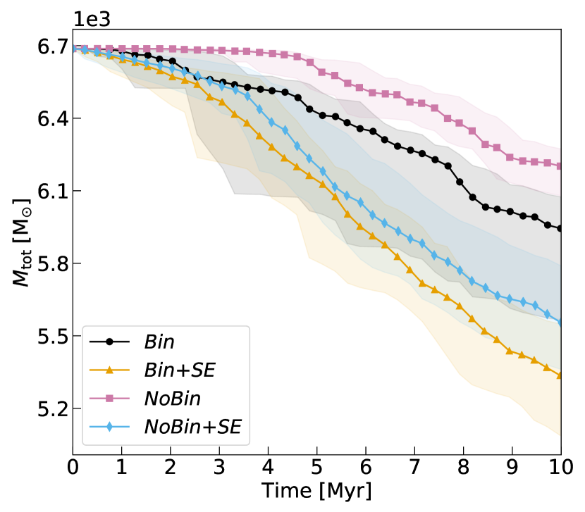
Figure 5: Mass variation in the four evolutionary cases we considered. Lines and colours are the same as in Fig. 4.

4.2.3 Mass loss

As the cluster expands, stars get further away from its centre, until they are eventually removed from the cluster dynamics by the tidal field of the host galaxy. This makes the total mass of the stellar system decrease. The presence of binary stars enhances the number of escaping stars, by powering a faster expansion. Also, close interactions between binary stars and single (or other binary) stars may lead to the ejection of stars, and possibly also of binary systems. In addition, stellar evolutionary processes (e.g. stellar winds, supernova explosions) make single stars, and thus the cluster, lose mass.

Figure 5 shows the variation of the total mass of the cluster. Stellar evolution gives the main contribution to mass loss in the early stages of the simulation, resulting in a steeper slope of the mass evolution. After $10\,\mathrm{Myr}$, the mass loss in the cases with stellar evolution is twice as large as that in the cases without stellar evolution. The absence of primordial binaries delays the mass loss, because the cluster needs to form its binaries dynamically before they start ejecting other stars.

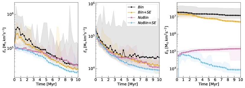
Figure 6: Evolution of the total kinetic energy ($E_{\rm k}$, left), of the total gravitational energy of the centres of mass ($E_{\rm g}$, middle) and of the total binding energy of the binary systems ($E_{\rm b}$, right). Lines and colours are the same as in Fig. 4.

4.2.4 Energy variation

Figure 6 shows the evolution of the total kinetic energy ($E_{\mathrm{k}}$), the total potential energy ($E_{\mathrm{g}}$) of the centres of mass and the total binding energy of binary systems ($E_{\mathrm{b}}$). Binary stars produce an initial sharp increase of the kinetic energy by yielding their internal energy to the surrounding stars. This results in the fast cluster expansion seen in Fig. 4. After this initial sharp increase, the kinetic energy of the clusters with original binaries decreases at a fast rate as a consequence of the ejection or evaporation of high velocity stars. After the first $\sim{}5$ Myr, the kinetic energy of the star clusters with original binary systems becomes similar to that of the other clusters, and they evolve in the same way for the rest of the simulation.

The total binding energy of the initial binary population is much higher than the typical gravitational energy of the centres of mass. Our original binary stars are, in fact, mostly hard and a small fraction of their total internal energy is sufficient to deeply affect the evolution of the cluster. The decrease of the total binding energy springs from two factors. Firstly, some binary stars escape from the system. This causes the slow decrease of the black line in Fig. 6. Secondly, stellar and binary evolution tend to remove binary stars from the population, via mergers, supernova explosions but also direct collisions between stars. This process is important since the very first stages, because the binary fraction is very high for the most massive stars and because the initial semi-major axes from Sana et al. (2012) are skewed to small values. By comparing the Bin models and the Bin+SE models, one can infer that this second factor is the main responsible for the variation of the total binding energy.

If there are no original binary systems (NoBin and NoBin+SE models), the cluster creates its own population, with binding energies of the order of the gravitational energy scale. The case without stellar evolution is characterized by a monotonic increase of the binding energy, where binaries form and the hardest ones tend to harden. In the end, the total binding energy is dominated by the binding energy of a very few binaries. In presence of stellar and binary evolution, after an initial increase, the total binding energy decreases when stellar and binary evolution processes take over.

4.3 Binary populations

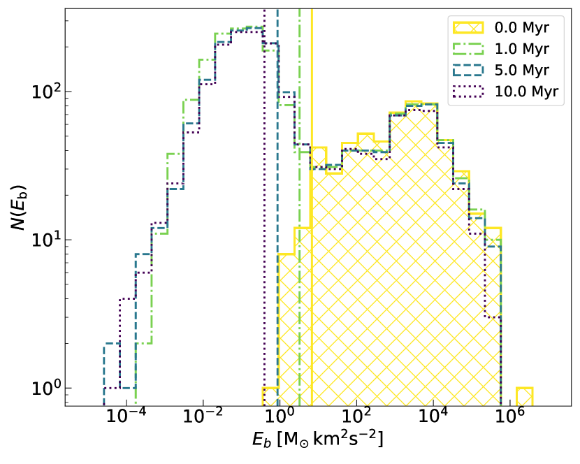
Figure 7: Distribution of binding energies for a cluster, in presence of original binaries and stellar evolution. Four different snapshots are shown: $t=0$ Myr (yellow solid line, hatched area), $t=1$ Myr (green dot-dashed line), $t=5$ Myr (blue dashed line), $t=10$ Myr (purple dotted line). The vertical lines represent the mean kinetic energy of the cluster, defined as the mean kinetic energy of the centres of mass within two half-mass radii (where binaries are more likely to interact).

In order to understand how binary populations evolve and interact with the host cluster, we must estimate how their binding energy distribution is related to the mean energy of the cluster. Figure 7 shows the distribution of binding energies for one representative simulation at four different snapshots, in presence of original binary systems and stellar evolution.

At the beginning of the simulation, binding energies are very large if compared to the mean kinetic energy. In particular, the hardest part of the distribution is about five orders of magnitude higher than the typical energy scale of the star cluster. This means that the other stars in the cluster "see" the hardest binary systems as if they were single stars: the cross section of the hardest binary systems is so small that these can hardly interact with single stars.

In absence of original binary systems with a sufficiently large cross section, the star cluster creates new binary systems, with a larger semi-major axis and, thus, a large cross section for three-body encounters. This is the reason behind the large number of binary systems created at successive snapshots, that are close to the mean kinetic energy of the cluster. Finally, the loosely bound tail of the binary distribution consists of soft binaries that are continuously created and destroyed by dynamical interactions with their neighbours.

Figure 8: Distribution of semi-major axes (left), mass ratios (centre) and multiplicity fractions (right) for a cluster with (upper panels) and without (lower panels) original binaries. Four different snapshots are shown: $t=0$ Myr (yellow solid line, hatched area, circles), $t=1$ Myr (green dot-dashed line, squares), $t=5$ Myr (blue dashed line, triangles), $t=10$ Myr (purple dotted line, diamonds).

4.3.1 Orbital parameters and multiplicity fraction

Figure 8 shows the evolution of probability density function (PDF) of the binary semi-major axes and of the mass ratios and the multiplicity fraction, defined as the sum of the fraction of binaries and the fraction of triples. We consider two representative populations, one for simulations with original binaries (the same as in Fig. 7) and one for simulations without original binaries, in presence of stellar evolution.

In presence of original binaries, the PDFs significantly change with time, because of the creation of a large number of dynamical binaries. In particular, the distribution of semi-major axes extends to higher values, and shows a secondary peak at $10^{3}$ AU, the typical value at which dynamical binaries form. This value corresponds to $\approx{}5\times 10^{-3}$ pc, that is the lowest distance scale (it is the typical distance of stars split into Plummer spheres). As explained above, the cluster responds to the absence of interacting binaries by creating its own. This also explains why the distributions of the dynamically formed semi-major axes and mass ratios are very similar to those that form in absence of original binaries (as shown in the lower-left panel of Fig. 8).

As for the mass ratios’ ($q$) distribution, dynamical interactions produce a steep increase of the PDF at high values, because the new binaries are typically formed by the low mass stars in the Plummer spheres. Also, the distribution of mass ratios extends towards lower values than the initial lower limit ($q=0.1$). Most of the variations in the PDFs take place in the first 1 Myr, that is when the environment is dynamically active. Since then, the binary distributions remain almost unchanged. Also, the large number of dynamically-created small-mass binaries increases the total multiplicity fraction from $\approx 6\%$ to $\approx 26\%$. In particular, these systems populate the lowest mass bin of Figure 1, by increasing the binary fraction from 0 to $20\%$.

In the absence of original binaries (NoBin+SE case), dynamical interactions produce a distribution of semi-major axes that is similar to the distribution of dynamically formed binary systems in the Bin+SE case, but cannot reproduce the hardest part of the Sana et al. (2012) binary distribution. Also, dynamical mechanisms tend to create equal-mass binaries. Remarkably, the binary fraction of dynamically formed binaries in the NoBin+SE case is mass-dependent: it grows with the mass of the primary star and mimics the trend of the observed distribution (Moe & Di Stefano, 2017). Hence, in the absence of original binary stars, the cluster is able to produce a mass-dependent binary fraction. However, there is not sufficient energy at small scales to reproduce the hardest part of the initial distribution of Sana et al. (2012).

4.3.2 Exchanges

The degree of interactions between the binary systems and their host cluster can be quantified by evaluating the number of exchanges that take place. Fig. 9 shows the variation of the incremental number of exchanges. The original binaries take part in a limited number of exchanges, most of which are in the first 2 Myr of the cluster’s life, when densities allow an efficient interaction with the other stars. In the following evolution, the original binaries interact much less, as indicated by the flatness of the curve. Nonetheless, because the original binaries are very hard, the few interactions they undergo exchange a sufficient amount of energy to affect the global evolution of the cluster, as shown by the evolution of $r_{50}$ (Fig. 4).

Interestingly, the total number of exchanges is about two orders of magnitude higher than that of original binaries and does not depend on the presence of an initial population of binary stars. This aspect indicates that the cluster under consideration is a very active environment for binary interactions and confirms that the most interacting binaries are dynamically created by the cluster itself. However, most of these exchanges involve binaries that are loosely bound (see also Fig. 7) and thus their energy exchange is quite low with respect to that of the original binaries.

Figure 9: Number of exchanges $N_{\rm exch}$ as a function of time for the entire population of binaries (solid lines, filled markers) and for the sub-population of original binaries (dashed lines, empty markers). $N_{\rm exch}$ is calculated at steps of 0.25 Myr. Lines and colours are the same as in Fig. 4.

4.4 Comparison with other initial conditions

The novelty of the Hydro initial conditions can be better understood if we compare their evolution to that of other, more idealized initial conditions. To this purpose, we ran simulations with the initial conditions presented in Section 3.1. Since we want to focus on the dynamical evolution with different initial phase-space distributions, we decided to run these simulations without stellar evolution.

Figure 10: Early evolution of the 50% Lagrangian radius (left-hand panel), the 10% Lagrangian radius (central panel), and the concentration of the cluster, quantified by $r_{\mathrm{50}}/r_{\mathrm{10}}$ (right-hand panel). Different lines represent the medians of different initial phase-space distributions: Hydro (yellow circles), King (pink squares), Loose Fract (purple triangles), Dense Fract (blue diamonds). The solid lines and filled markers represent clusters with original binaries, while the dashed lines and empty markers correspond to clusters without original binaries.

4.4.1 Cluster Expansion

Figure 10 shows the evolution of the medians of the distributions of $r_{50}$, of $r_{10}$, and of the ratio $r_{50}/r_{10}$, that measures the concentration of the system. In the initial conditions, the Hydro clusters have a much larger ratio $r_{50}/r_{10}$ than the other models. Hence, they have very dense cores and rather extended halos, because of the scale of the sub-structures. For these intrinsic differences, the evolution of the characteristic radii of the Hydro simulations is considerably different from that of the other distributions.

In the first Myr, the Hydro case is the only one that does not show a monotonic increase of $r_{50}$ because of the initial sub-cluster motion (as discussed in Section 4.2.1). All of the other initial conditions present a monotonic increase of $r_{50}$ and $r_{10}$, but with different slopes. The Loose Fract case, that is initialized with the same half-mass radius as the Hydro case, shows a mild expansion on both scales, due to its supervirial state. The low density of the central regions (the initial value of $r_{10}$ is larger than in the Hydro case by a factor of 5, see Tab. 1) does not allow efficient star-star interactions, that would power a faster expansion. The King and Dense Fract models, that are set to match the core radius of the initial Hydro simulations, undergo a stronger expansion from the very beginning of their evolution. These two different initial conditions present a very similar behavior.

The peculiarity in the evolution of the Hydro case is evident when the evolution of the ratio $r_{50}/r_{10}$ is taken into account. All the cases except the Hydro present a monotonic slow decrease for the $r_{50}/r_{10}$ ratio, that indicates that the systems expand at a similar rate at both scales. The Hydro initial conditions, instead, show an initial steep decrease, because the growth of $r_{\mathrm{50}}$ is balanced by the sub-clump motion (see Fig. 4), while at smaller scales the cluster expands rapidly. Even when it has reached a nearly monolithic shape, the evolution of its $r_{50}/r_{10}$ ratio is very different from the other initial conditions: this ratio rapidly increases until it reaches a maximum at about 5 Myr. Such a difference may be explained in terms of the stronger mass segregation that features the Hydro simulation (we will discuss this point in Sect. 5).

4.4.2 Binding energies

Figure 11: Evolution of the total binding energy of the binary systems. Lines and colours are the same as Fig. 10.

Figure 11 shows the evolution of the total binding energy for different initial conditions. In absence of original binaries, every initial configuration creates its own population and the resulting total binding energy is strictly connected to the initial energy scale of the system. In particular, the Hydro, King and Dense Fract final binding energies are similar to each other as they are initialized with similar core radii, whereas the total binding energy of the Loose Fract systems is about one order of magnitude lower. Most of the total binding energy is contained in a limited number of binaries (from 2 to 5) that go on hardening as the simulation proceeds. This relation between the total binding energy and the global scales of the clusters confirms that star clusters are self-regulating systems with respect to their binary populations (Goodman & Hut, 1989, 1993): in absence of binaries, each system creates its own population of binaries, with binding energies of the order of its global energy scales.

5 Discussion

The Hydro star clusters present a very distinctive evolution of the $r_{\mathrm{50}}/r_{\mathrm{10}}$ ratio. We studied what factor determines the growth of this ratio during the monolithic phase. In particular, we focus on the impact of the initial degree of mass segregation. In fact, a high degree of mass segregation would allow the most massive stars to rapidly form a centrally concentrated core that is dynamically separated from the rest of the cluster, the scenario usually referred to as Spitzer instability (Spitzer, 1969). If this happens, the distribution of massive stars is hotter than the rest of the cluster, because they remain more concentrated and the local value of the velocity dispersion decreases with the distance from the centre.

Previous N$-$body simulations have found evidence that, for a wide range of initial conditions, the most massive stars in a system do not move slower than the low-mass stars (Parker & Wright, 2016; Spera et al., 2016; Webb & Vesperini, 2017), as one would expect based on the tendency of stellar systems towards energy equipartition (Trenti & van der Marel, 2013; Bianchini et al., 2016). A confirmation that the most massive stars can present higher velocities has also been found in proper motion observations of the open cluster NGC 6530 (Wright et al., 2019). Wright & Parker (2019) showed that this aspect can be explained by the combination of Spitzer instability and a cool collapse. If the most massive stars remain more concentrated than the rest of cluster, then the core, that is mostly populated by these massive stars, is expected to expand slower than the rest of the cluster.

To quantify the impact of mass segregation on the evolution of the cluster, we selected the 30 most massive stellar particles and evaluated the ratio between their velocity dispersion $\sigma_{\mathrm{mass}}$ and the velocity dispersion of all the stellar particles $\sigma_{\mathrm{all}}$. For these calculation, only stars inside two half-mass radii are considered, as done in Wright & Parker (2019). The evolution of the ratio between these two velocity dispersions is shown in the upper panel Fig. 12. In all the phase-space configurations except the Hydro, the velocity dispersion ratio is about one and does not change very much with time. In the Hydro case, instead, the high initial value of the velocity dispersion ratio suggests that the stellar cluster presents a strong initial mass segregation. Also, during the monolithic phase, the velocity dispersion ratio grows because, after the merger of the two main sub-clumps, their most massive stars rapidly segregate towards the centre, while the system globally expands. The segregation of the massive stars towards the centre of the potential well may be enhanced by the fact that, in each sub-clump, the stars have already formed a massive core that segregates as one single, very massive particle. In the case with binaries, the velocity dispersion value grows enough to match the observed value for NGC 6530.

The connection between the growth of the velocity dispersion ratio and the degree of mass segregation is confirmed by the trend shown by the ratio of the half-mass radii of the 30 most massive stellar particles $r_{\rm mass}$ and the overall half-mass radius $r_{\rm 50}$, shown in the bottom panel of Fig. 12. The Hydro simulations show an initial strong degree of mass segregation. The initial small scale expansion makes this ratio instantly grow; but, then, it rapidly decreases because of the strong segregation at the centre of the cluster. The initial degree of mass segregation seems to be the most important factor in the growth of the velocity dispersion ratio in the Hydro case: a stronger initial degree of mass segregation triggers the rapid formation of a dense core that expands more slowly than the rest of the cluster. Also, the rapid formation of a dense core could influences the interaction rate between binaries and the host cluster. If the primordial hard binaries live in a denser environment, they are more likely to interact: this explains why the Hydro initial conditions present different expansions for the cases with and without binaries (Fig. 10).

Figure 12: Upper panel: evolution of the ratio between the velocity dispersion of the 30 most massive star particles $\sigma_{\rm mass}$ and the velocity dispersion of all the stars inside inside $2\,r_{50}$, $\sigma_{\rm all}$. The grey data point with error bar is the observed value for NGC 6530 (Wright et al., 2019). Lower panel: evolution of the ratio between the half-mass radius of the 30 most massive star particles ($r_{\rm mass}$) and the overall half-mass radius, $r_{50}$. Lines and colours are the same as Fig. 10.

6 Summary and Conclusions

We studied the early dynamical evolution ($t<10\,\mathrm{Myr}$) of young stellar clusters with realistic populations of binaries and different initial phase-space distributions. The initial conditions for our N$-$body simulations are obtained by combining a new algorithm to generate realistic stellar and binary distributions (Sana et al., 2012; Moe & Di Stefano, 2017) with the joining/splitting algorithm defined in Ballone et al. (2021), to derive initial conditions from hydrodynamical simulations.

For the hydrodynamical initial conditions (Hydro cluster), we considered different evolutionary cases by switching on and off the presence of original binary stars and stellar evolution in order to weight their contribution to the dynamical evolution. Our results show that the evolution of the cluster is characterized by two distinct evolutionary phases: first, the global expansion of the cluster is balanced by the approaching of its main sub-clumps, while at small scales the cluster expands instantaneously. After 1 Myr, the cluster has reached a nearly monolithic shape and expands as a whole, following a post-core collapse expansion. Binaries tend to speed up the expansion of the cluster in this phase, making the half-mass radius expand faster, while stellar evolution has a minor impact on the early dynamical evolution of the cluster, but has a major impact on mass loss.

We compared the evolution of the Hydro star cluster to that of star clusters with spherical distributions of stars (King, Loose Fract, Dense Fract). The main difference between the Hydro cluster and the others relies in the evolution of the $r_{50}/r_{10}$ ratio, that measures the concentration of the system. The Hydro cluster, in fact, shows a distinctive trend of $r_{50}/r_{10}$. At the beginning of the simulations, $r_{50}/r_{10}$ is much larger in the Hydro cluster than in the other models, because the Hydro cluster is an aggregate of several sub-clumps, resulting in a large total half-mass radius, but its core radius is very small, since it basically coincides with the core radius of the densest sub-clump. The $r_{50}/r_{10}$ ratio decreases very fast ($<1$ Myr) in the Hydro cluster, reaching values similar to the other clusters, because of the hierarchical merger of the sub-clumps, which reduces the total half-mass radius. However, at $t>1$ Myr the value of $r_{50}/r_{10}$ keeps decreasing in the spherical models, while it grows again in the Hydro case. The late growth of $r_{50}/r_{10}$ in the Hydro cluster is due to its initial high degree of mass segregation, which allows it to form a centrally concentrated core of massive stars. As this core expands more slowly than the rest of the cluster, the ratio between the velocity dispersion of the most massive stars and that of all the stars increases. In the case with binaries, it grows enough to match the observed value for NGC 6530 (Wright et al., 2019).

The initial binary stars we set based on observational constraints (Sana et al., 2012; Moe & Di Stefano, 2017) are generally too hard to interact in an efficient way with the host environment. The stellar systems recover from the lack of interacting binaries by dynamically creating additional binaries with binding energy of the order of their kinetic energy. Also, in the absence of primordial binaries, the binary fraction of the dynamically formed binaries show a binary fraction that increases with the mass of the primary star. This behaviour spontaneously reproduces the relation between binary fraction and stellar mass found in observations (Moe & Di Stefano, 2017).

Data availability

The data underlying this article will be shared on reasonable request to the corresponding authors.

References

- Abbott et al. (2020a) Abbott R., et al., 2020a, arXiv e-prints, p. arXiv:2010.14527
- Abbott et al. (2020b) Abbott R., et al., 2020b, arXiv e-prints, p. arXiv:2010.14533
- Allison et al. (2010) Allison R. J., Goodwin S. P., Parker R. J., Portegies Zwart S. F., de Grijs R., 2010, MNRAS, 407, 1098
- Anders & Grevesse (1989) Anders E., Grevesse N., 1989, Geochimica Cosmochimica Acta, 53, 197
- Antonini & Gieles (2020) Antonini F., Gieles M., 2020, MNRAS, 492, 2936
- Ballone et al. (2020) Ballone A., Mapelli M., Di Carlo U. N., Torniamenti S., Spera M., Rastello S., 2020, MNRAS, 496, 49
- Ballone et al. (2021) Ballone A., Torniamenti S., Mapelli M., Di Carlo U. N., Spera M., Rastello S., Gaspari N., Iorio G., 2021, MNRAS, 501, 2920
- Banerjee (2017) Banerjee S., 2017, MNRAS, 467, 524
- Banerjee & Kroupa (2013) Banerjee S., Kroupa P., 2013, ApJ, 764, 29
- Banerjee et al. (2010) Banerjee S., Baumgardt H., Kroupa P., 2010, MNRAS, 402, 371
- Bate et al. (1995) Bate M. R., Bonnell I. A., Price N. M., 1995, MNRAS, 277, 362
- Baumgardt & Kroupa (2007) Baumgardt H., Kroupa P., 2007, MNRAS, 380, 1589
- Bianchini et al. (2013) Bianchini P., Varri A. L., Bertin G., Zocchi A., 2013, ApJ, 772, 67
- Bianchini et al. (2016) Bianchini P., van de Ven G., Norris M. A., Schinnerer E., Varri A. L., 2016, MNRAS, 458, 3644
- Bianchini et al. (2018) Bianchini P., van der Marel R. P., del Pino A., Watkins L. L., Bellini A., Fardal M. A., Libralato M., Sills A., 2018, MNRAS, 481, 2125
- Boley (2009) Boley A. C., 2009, ApJ, 695, L53
- Burgers (1948) Burgers J. M., 1948, Advances in Applied Mechanics, 1, 171
- Cantat-Gaudin et al. (2019) Cantat-Gaudin T., et al., 2019, A&A, 626, A17
- Cartwright & Whitworth (2004) Cartwright A., Whitworth A. P., 2004, MNRAS, 348, 589
- Chatterjee et al. (2013) Chatterjee S., Umbreit S., Fregeau J. M., Rasio F. A., 2013, MNRAS, 429, 2881
- Chevance et al. (2020a) Chevance M., et al., 2020a, arXiv e-prints, p. arXiv:2010.13788
- Chevance et al. (2020b) Chevance M., et al., 2020b, MNRAS, 493, 2872
- Cournoyer-Cloutier et al. (2020) Cournoyer-Cloutier C., et al., 2020, arXiv e-prints, p. arXiv:2011.06105
- Daffern-Powell & Parker (2020) Daffern-Powell E. C., Parker R. J., 2020, MNRAS, 493, 4925
- Dale et al. (2014) Dale J. E., Ngoumou J., Ercolano B., Bonnell I. A., 2014, MNRAS, 442, 694
- Di Carlo et al. (2019) Di Carlo U. N., Giacobbo N., Mapelli M., Pasquato M., Spera M., Wang L., Haardt F., 2019, MNRAS, 487, 2947
- Di Carlo et al. (2020a) Di Carlo U. N., Mapelli M., Bouffanais Y., Giacobbo N., Santoliquido F., Bressan A., Spera M., Haardt F., 2020a, MNRAS, 497, 1043
- Di Carlo et al. (2020b) Di Carlo U. N., et al., 2020b, MNRAS, 498, 495
- Ebisuzaki et al. (2001) Ebisuzaki T., et al., 2001, ApJ, 562, L19
- Ester et al. (1996) Ester M., Kriegel H.-P., Sander J., Xu X., 1996. AAAI Press, pp 226–231
- Fryer et al. (2012) Fryer C. L., Belczynski K., Wiktorowicz G., Dominik M., Kalogera V., Holz D. E., 2012, ApJ, 749, 91
- Fujii (2015) Fujii M. S., 2015, PASJ, 67, 59
- Fujii & Portegies Zwart (2011) Fujii M. S., Portegies Zwart S., 2011, Science, 334, 1380
- Fujii & Portegies Zwart (2014) Fujii M. S., Portegies Zwart S., 2014, MNRAS, 439, 1003
- Fujii & Portegies Zwart (2015) Fujii M. S., Portegies Zwart S., 2015, MNRAS, 449, 726
- Fujii et al. (2017) Fujii M. S., Tanikawa A., Makino J., 2017, PASJ, 69, 94
- Fujii et al. (2021) Fujii M. S., Saitoh T. R., Hirai Y., Wang L., 2021, arXiv e-prints, p. arXiv:2103.02829
- Gavagnin et al. (2017) Gavagnin E., Bleuler A., Rosdahl J., Teyssier R., 2017, MNRAS, 472, 4155
- Giacobbo & Mapelli (2018) Giacobbo N., Mapelli M., 2018, MNRAS, 480, 2011
- Giacobbo & Mapelli (2019) Giacobbo N., Mapelli M., 2019, MNRAS, 482, 2234
- Giacobbo & Mapelli (2020) Giacobbo N., Mapelli M., 2020, ApJ, 891, 141
- Giacobbo et al. (2018) Giacobbo N., Mapelli M., Spera M., 2018, MNRAS, 474, 2959
- Giersz et al. (2015) Giersz M., Leigh N., Hypki A., Lützgendorf N., Askar A., 2015, MNRAS, 454, 3150
- Goodman & Hut (1989) Goodman J., Hut P., 1989, Nature, 339, 40
- Goodman & Hut (1993) Goodman J., Hut P., 1993, ApJ, 403, 271
- Goodwin & Bastian (2006) Goodwin S. P., Bastian N., 2006, MNRAS, 373, 752
- Goodwin & Whitworth (2004) Goodwin S. P., Whitworth A. P., 2004, A&A, 413, 929
- Heggie (1975) Heggie D. C., 1975, MNRAS, 173, 729
- Hénault-Brunet et al. (2012) Hénault-Brunet V., et al., 2012, A&A, 545, L1
- Hills (1980) Hills J. G., 1980, ApJ, 235, 986
- Hurley et al. (2000) Hurley J. R., Pols O. R., Tout C. A., 2000, MNRAS, 315, 543
- Hurley et al. (2002) Hurley J. R., Tout C. A., Pols O. R., 2002, MNRAS, 329, 897
- Hut (1981) Hut P., 1981, A&A, 99, 126
- Hut (1983) Hut P., 1983, ApJ, 272, L29
- Kamann et al. (2018) Kamann S., et al., 2018, MNRAS, 473, 5591
- King (1966) King I. R., 1966, AJ, 71, 64
- Kroupa (2001) Kroupa P., 2001, MNRAS, 322, 231
- Kudritzki (2002) Kudritzki R. P., 2002, ApJ, 577, 389
- Kuhn et al. (2019) Kuhn M. A., Hillenbrand L. A., Sills A., Feigelson E. D., Getman K. V., 2019, ApJ, 870, 32
- Kumamoto et al. (2019) Kumamoto J., Fujii M. S., Tanikawa A., 2019, MNRAS, 486, 3942
- Küpper et al. (2011) Küpper A. H. W., Maschberger T., Kroupa P., Baumgardt H., 2011, MNRAS, 417, 2300
- Larson (1995) Larson R. B., 1995, MNRAS, 272, 213
- Makino & Aarseth (1992) Makino J., Aarseth S. J., 1992, PASJ, 44, 141
- Mapelli (2016) Mapelli M., 2016, MNRAS, 459, 3432
- Mapelli (2017) Mapelli M., 2017, MNRAS, 467, 3255
- Mapelli & Giacobbo (2018) Mapelli M., Giacobbo N., 2018, MNRAS, 479, 4391
- Mapelli et al. (2020) Mapelli M., Spera M., Montanari E., Limongi M., Chieffi A., Giacobbo N., Bressan A., Bouffanais Y., 2020, ApJ, 888, 76
- Marks & Kroupa (2012) Marks M., Kroupa P., 2012, A&A, 543, A8
- Mikkola & Aarseth (1993) Mikkola S., Aarseth S. J., 1993, Celestial Mechanics and Dynamical Astronomy, 57, 439
- Moe & Di Stefano (2017) Moe M., Di Stefano R., 2017, ApJS, 230, 15
- Moeckel & Bate (2010) Moeckel N., Bate M. R., 2010, MNRAS, 404, 721
- Moeckel et al. (2012) Moeckel N., Holland C., Clarke C. J., Bonnell I. A., 2012, MNRAS, 425, 450
- Moyano Loyola & Hurley (2013) Moyano Loyola G. R. I., Hurley J. R., 2013, MNRAS, 434, 2509
- Nitadori & Aarseth (2012) Nitadori K., Aarseth S. J., 2012, MNRAS, 424, 545
- Pancino et al. (2007) Pancino E., Galfo A., Ferraro F. R., Bellazzini M., 2007, ApJ, 661, L155
- Pang et al. (2020) Pang X., Li Y., Tang S.-Y., Pasquato M., Kouwenhoven M. B. N., 2020, ApJ, 900, L4
- Parker & Dale (2013) Parker R. J., Dale J. E., 2013, MNRAS, 432, 986
- Parker & Meyer (2012) Parker R. J., Meyer M. R., 2012, MNRAS, 427, 637
- Parker & Wright (2016) Parker R. J., Wright N. J., 2016, MNRAS, 457, 3430
- Parker et al. (2014) Parker R. J., Wright N. J., Goodwin S. P., Meyer M. R., 2014, MNRAS, 438, 620
- Pedregosa et al. (2011) Pedregosa F., et al., 2011, Journal of Machine Learning Research, 12, 2825
- Pelupessy et al. (2013) Pelupessy F. I., van Elteren A., de Vries N., McMillan S. L. W., Drost N., Portegies Zwart S. F., 2013, A&A, 557, A84
- Pfalzner (2009) Pfalzner S., 2009, A&A, 498, L37
- Pfalzner et al. (2014) Pfalzner S., Parmentier G., Steinhausen M., Vincke K., Menten K., 2014, ApJ, 794, 147
- Plummer (1911) Plummer H. C., 1911, MNRAS, 71, 460
- Portegies Zwart & Verbunt (1996) Portegies Zwart S. F., Verbunt F., 1996, A&A, 309, 179
- Portegies Zwart et al. (2004) Portegies Zwart S. F., Baumgardt H., Hut P., Makino J., McMillan S. L. W., 2004, Nature, 428, 724
- Portegies Zwart et al. (2010) Portegies Zwart S. F., McMillan S. L. W., Gieles M., 2010, ARA&A, 48, 431
- Sabbi et al. (2012) Sabbi E., et al., 2012, ApJ, 754, L37
- Sana et al. (2012) Sana H., et al., 2012, Science, 337, 444
- Sánchez & Alfaro (2009) Sánchez N., Alfaro E. J., 2009, ApJ, 696, 2086
- Schmeja & Klessen (2006) Schmeja S., Klessen R. S., 2006, A&A, 449, 151
- Spera et al. (2016) Spera M., Mapelli M., Jeffries R. D., 2016, MNRAS, 460, 317
- Spitzer (1969) Spitzer Lyman J., 1969, ApJ, 158, L139
- Spitzer (1987) Spitzer L., 1987, Dynamical evolution of globular clusters
- Spitzer & Hart (1971) Spitzer Lyman J., Hart M. H., 1971, ApJ, 164, 399
- Stiefel et al. (1965) Stiefel E. L., Rheinboldt W. C., Rheinboldt C. J., Hagger H. J., 1965, Physics Today, 18, 110
- Takahashi & Baumgardt (2012) Takahashi K., Baumgardt H., 2012, MNRAS, 420, 1799
- Trani et al. (2021) Trani A. A., Tanikawa A., Fujii M. S., Leigh N. W. C., Kumamoto J., 2021, arXiv e-prints, p. arXiv:2102.01689
- Trenti & van der Marel (2013) Trenti M., van der Marel R., 2013, MNRAS, 435, 3272
- Vázquez-Semadeni et al. (2010) Vázquez-Semadeni E., Colín P., Gómez G. C., Ballesteros-Paredes J., Watson A. W., 2010, ApJ, 715, 1302
- Vink et al. (2001) Vink J. S., de Koter A., Lamers H. J. G. L. M., 2001, A&A, 369, 574
- Wadsley et al. (2004) Wadsley J. W., Stadel J., Quinn T., 2004, New Astron., 9, 137
- Wadsley et al. (2017) Wadsley J. W., Keller B. W., Quinn T. R., 2017, MNRAS, 471, 2357
- Wang et al. (2015) Wang L., Spurzem R., Aarseth S., Nitadori K., Berczik P., Kouwenhoven M. B. N., Naab T., 2015, MNRAS, 450, 4070
- Wang et al. (2016) Wang L., et al., 2016, MNRAS, 458, 1450
- Webb & Vesperini (2017) Webb J. J., Vesperini E., 2017, MNRAS, 464, 1977
- Webbink (1984) Webbink R. F., 1984, ApJ, 277, 355
- Wright & Parker (2019) Wright N. J., Parker R. J., 2019, MNRAS, 489, 2694
- Wright et al. (2019) Wright N. J., et al., 2019, VizieR Online Data Catalog, p. J/MNRAS/486/2477
- Ziosi et al. (2014) Ziosi B. M., Mapelli M., Branchesi M., Tormen G., 2014, MNRAS, 441, 3703
- van Leeuwen et al. (2000) van Leeuwen F., Le Poole R. S., Reijns R. A., Freeman K. C., de Zeeuw P. T., 2000, A&A, 360, 472