Turnaround radius in $\Lambda$CDM, and dark matter cosmologies II: the role of dynamical friction

Abstract

This paper is an extension of the paper by Del Popolo, Chan, and Mota (2020) to take account the effect of dynamical friction. We show how dynamical friction changes the threshold of collapse, $\delta_{c}$, and the turn-around radius, $R_{t}$. We find numerically the relationship between the turnaround radius, $R_{\rm t}$, and mass, $M_{\rm t}$, in $\Lambda$CDM, in dark energy scenarios, and in a $f(R)$ modified gravity model. Dynamical friction gives rise to a $R_{\rm t}-M_{\rm t}$ relation differing from that of the standard spherical collapse. In particular, dynamical friction amplifies the effect of shear, and vorticity already studied in Del Popolo, Chan, and Mota (2020). A comparison of the $R_{\rm t}-M_{\rm t}$ relationship for the $\Lambda$CDM, and those for the dark energy, and modified gravity models shows, that the $R_{\rm t}-M_{\rm t}$ relationship of the $\Lambda$CDM is similar to that of the dark energy models, and small differences are seen when comparing with the $f(R)$ models. The effect of shear, rotation, and dynamical friction is particularly evident at galactic scales, giving rise to a difference between the $R_{\rm t}-M_{\rm t}$ relation of the standard spherical collapse of the order of $\simeq 60\%$. Finally, we show how the new values of the $R_{\rm t}-M_{\rm t}$ influence the constraints to the $w$ parameter of the equation of state.

I Introduction

In the past several decades, observations revealed that some missing mass exist in our universe Sanders (2010). Many physicists believe that the existence of some unknown particles called cold dark matter (CDM) can account for the missing mass Profumo (2017). On the other hand, cosmological observations suggest that the expansion of our universe is accelerating. Many cosmologists propose that the existence of a new kind of energy called dark energy can help explain the accelerating expansion Li et al. (2011). In standard cosmological model, the amount of dark energy can be represented by the cosmological constant $\Lambda$. This standard cosmological model is now known as the $\Lambda$CDM model. The $\Lambda$CDM model can give good agreements for observations in large-scale structures Del Popolo (2013); Ade (2016). However, there are some discrepancies between the predictions of the $\Lambda$CDM model and the observations in small-scale structures. Specifically, the core-cusp problem de Blok (2010), the missing satellites problem Moore et al. (1999) and the mass-discrepancy acceleration relation problem McGaugh (2004); McGaugh et al. (2016) are three classical problems challenging the $\Lambda$CDM model. Moreover, currently no compelling particle dark matter signal has been detected directly or indirectly. The current direct-detection and indirect-detection constraints of dark matter have ruled out a large parameter space of potential particle dark matter models Aprile (2017); Abecrcrombie (2020); Ackermann (2015); Chan and Leung (2017); Chan et al. (2019); Chan and Lee (2020). Also, the cosmological constant $\Lambda$ suffers from the cosmological constant fine-tuning problem and the cosmic coincidence problem Weinberg (1989); Velten et al. (2014). Therefore, despite some success in the cosmological scale, the $\Lambda$CDM model is still being challenged by many recent studies.

Based on the above problems, some studies propose alternative models for the universe accelerated expansion. Dark energy (DE) effects are generated by additional matter fields (e.g., quintessence (Copeland et al., 2006)), or that the dynamical effects of dark matter and/or dark energy might originate from modified gravity (MG) models(Horndeski, 1974; Milgrom, 1983; Zwiebach, 1985; Moffat, 2006; Nojiri et al., 2005; Bekenstein, 2010; De Felice and Tsujikawa, 2010; Linder, 2010; Milgrom, 2014; Lovelock, 1971; Hořava, 2009; Rodríguez and Navarro, 2017; Horndeski, 1974; Deffayet et al., 2010, 2010)

Several popular modified gravity theories have been proposed to compete with the standard $\Lambda$CDM model, including Emergent Gravity Verlinde (2017), f(R) gravity Buchdahl (1970) and scalar-tensor-vector gravity Moffat (2006). Therefore, it is very important to motivate some theoretical framework to differentiate the dynamical effects of the $\Lambda$CDM model and the modified gravity. Some recent studies proposed that using the turnaround radius (TAR) can be a clue to test the standard $\Lambda$CDM model and modified gravity models Bhattacharya et al. (2017); Lopes et al. (2018, 2019); Pavlidou and Tomaras (2014); Pavlidou et al. (2014); Faraoni et al. (2015). The TAR has been claimed to be a well-defined and unambiguous boundary of a structure (e.g. galaxy clusters) in simulations Pavlidou and Tomaras (2014). Different cosmological models and modified gravity models might have different general relations of the TAR. Therefore, determining the TAR of different structures precisely would be crucial to test and constrain different cosmological models (Lopes et al., 2018), DE, and disentangle between $\Lambda$CDM model, DE, and MG models (Pavlidou and Tomaras, 2014; Pavlidou et al., 2014; Faraoni et al., 2015; Bhattacharya et al., 2017; Lopes et al., 2018, 2019).

Contrarily to the previous claim, we already showed in (Del Popolo et al., 2013a, b; Pace et al., 2014a; Mehrabi et al., 2017; Pace et al., 2019; Del Popolo et al., 2020) that shear, and vorticity modifies the non-linear evolution of structures. In this paper, we will also show that dynamical friction further modifies the structure formation, and consequently modifies TAR, and that TAR generally depends on baryons physics Del Popolo et al. (2020). By using an extended spherical collapse model, the TAR depends on the effects of shear and vorticity. Taking into account of the effects of shear and vorticity, the relation between TAR and total mass can differ by 30% from that omit these effects, especially in galaxies Del Popolo et al. (2020). In the present paper, we show that the effect of dynamical friction is also significant.

TAR was calculated by (Pavlidou and Tomaras, 2014; Pavlidou et al., 2014) for the $\Lambda$CDM model smooth DE model, while (Faraoni et al., 2015) obtained TAR in generic gravitational theories.

In this paper, we extend the results of (Del Popolo et al., 2020), based on an extended spherical collapse model (ESCM) introduced, and adopted in (Del Popolo, 2013; Del Popolo et al., 2013a; Pace et al., 2014a; Mehrabi et al., 2017; Pace et al., 2019). The ESCM takes into account the effect of shear, vorticity and dynamical friction on the collapse, to show how the TAR is changed. Apart the typical parameters of the spherical collapse, shear, vorticity, and dynamical friction change the two-point correlation function (Del Popolo and Gambera, 1999), the weak lensing peaks (Pace et al., 2019), and the mass function (Del Popolo, 2013; Del Popolo et al., 2013a; Pace et al., 2014a; Mehrabi et al., 2017). Similarly, to (Del Popolo et al., 2020), the aim of the paper is to show how the parameters of the spherical collapse are changed, together with the $R_{\rm t}$-$M_{\rm t}$ relation for MG models, DE models, and to compare to $\Lambda$CDM model predictions.

The paper is organized as follows. Section II describes the model used to derive the $R_{\rm t}$-$M_{\rm t}$ relation. Section III is devoted to the discussion of our results. Section IV is devoted to conclusions.

II The Model

In the following, we will use an improved version (Fillmore and Goldreich, 1984; Bertschinger, 1985; Hoffman and Shaham, 1985; Ryden and Gunn, 1987; Subramanian et al., 2000; Ascasibar et al., 2004; Williams et al., 2004) of the spherical collapse model introduced by Gunn and Gott (1972). The model describes the evolution of perturbation from the linear to the non-linear phase, when them decouple from Hubble flow, reach a maximum radius, the TAR, collapse, and viriliaze forming a structure. As reported the initial model of Gunn and Gott (1972) was extended to take account of angular momentum (Ryden and Gunn, 1987; Gurevich and Zybin, 1988a, b; White and Zaritsky, 1992; Sikivie et al., 1997; Nusser, 2001; Hiotelis, 2002; Le Delliou and Henriksen, 2003; Ascasibar et al., 2004; Williams et al., 2004; Zukin and Bertschinger, 2010), of dynamical friction (Antonuccio-Delogu and Colafrancesco, 1994; Del Popolo, 2009), shear (Hoffman, 1986, 1989; Zaroubi and Hoffman, 1993), and the effects of the DE fluid perturbation (see Mota and van de Bruck, 2004; Nunes and Mota, 2006; Abramo et al., 2007, 2008, 2009a, 2009b; Creminelli et al., 2010; Basse et al., 2011; Batista and Pace, 2013). Del Popolo et al. (2013a, b) studied the effects of shear and rotation in smooth DE models, Pace et al. (2014b) in clustering DE cosmologies, and Del Popolo et al. (2013c) in Chaplygin cosmologies.

II.1 The ESCM

Here, we show how the evolution equations of $\delta$ in the non-linear regime can be obtained.

The equations of evolution of $\delta$ in the non-linear regime were obtained by Bernardeau (1994); Padmanabhan (1996); Ohta et al. (2003, 2004); Abramo et al. (2007); Pace et al. (2010). In order to obtain the equation, we used the Neo-Newtonian expressions for the relativistic Poisson equation, the Euler, and continuity equations (Lima et al., 1997)

$$\frac{\partial\rho}{\partial t}+\nabla_{\vec{r}}\cdot(\rho\vec{v})+\frac{P}{c^{2}}\nabla_{\vec{r}}\cdot\vec{v} = 0\;,$$ (1)

$$\frac{\partial\vec{v}}{\partial t}+(\vec{v}\cdot\nabla_{\vec{r}})\vec{v}+\nabla_{\vec{r}}\Phi+{\bf\frac{c^{2}}{c^{2}\rho+P}\nabla P} = 0\;,$$ (2)

$$\nabla^{2}\Phi-4\pi G\left(\rho+\frac{3P}{c^{2}}\right) = 0\;,$$ (3)

where the equation of state (EoS) is given by $P=w\rho c^{2}$, $\vec{r}$ indicates the physical coordinate, $\Phi$ the Newtonian gravitational potential, and $\vec{v}$ the velocity in three-space. Writing and combining the perturbation equation as in (Del Popolo et al., 2020), we obtain the non-linear evolution equation in a dust ($w=0$) universe

$$\begin{split}\ddot{\delta}+2H\dot{\delta}-\frac{4}{3}\frac{\dot{\delta}^{2}}{1+\delta}-4\pi G\bar{\rho}\delta(1+\delta)-\\ (1+\delta)(\sigma^{2}-\omega^{2})&=0\;\end{split}$$ (4)

Eq. (4) is Eq. 41 of Ohta et al. (2003), and a generalization of Eq. 7 of Abramo et al. (2007) to the case of a non-spherical configuration of a rotating fluid.

In Eq. (4), $H$ is the Hubble function, $\overline{\rho}=\rho-\delta\rho$ the background density, $\sigma^{2}=\sigma_{ij}\sigma^{ij}$, and $\omega^{2}=\omega_{ij}\omega^{ij}$ are the shear, and rotation term, respectively. The shear term is related to a symmetric traceless tensor, dubbed shear tensor, while rotation term is related to an antisymmetric tensor.

In terms of the scale factor, $a$, the nonlinear equation driving the evolution of the overdensity contrast can be rewritten as:

$$\begin{split}\delta^{\prime\prime}+\left(\frac{3}{a}+\frac{E^{\prime}}{E}\right)\delta^{\prime}-\frac{4}{3}\frac{\delta^{\prime 2}}{1+\delta}-\frac{3}{2}\frac{\Omega_{\mathrm{m},0}}{a^{5}E^{2}(a)}\delta(1+\delta)-&\\ \frac{1}{a^{2}H^{2}(a)}(1+\delta)(\sigma^{2}-\omega^{2})&=0\;,\end{split}$$ (5)

where $\Omega_{m,0}$ is DM density parameter at $t=0$ ($a=1$), and $E(a)$ is given in Eq. 11 of (Del Popolo et al., 2020).

Since $\delta=\frac{2GM_{\rm m}}{\Omega_{m,0}H^{2}_{0}}(a/R)^{3}-1$, where $R$ is the effective perturbation radius, inserting into Eq. (4), it is easy to check that the evolution equation for $\delta$ reduces to the spherical collapse model (SCM) (Fosalba and Gaztan̈aga, 1998; Engineer et al., 2000; Ohta et al., 2003)

$$\ddot{R} = -\frac{GM_{\rm m}}{R^{2}}-\frac{GM_{\rm de}}{R^{2}}(1+3w_{\rm de})-\frac{\sigma^{2}-\omega^{2}}{3}R=$$ (6)

$$-\frac{GM_{\rm m}}{R^{2}}-\frac{4\pi G\bar{\rho_{\rm de}}R}{3}(1+3w_{\rm de})-\frac{\sigma^{2}-\omega^{2}}{3}R\,,$$

where $M_{\rm de}$ is the mass of the dark-energy component enclosed in the volume, $M_{\rm m}=\frac{4\pi R^{3}}{3}(\bar{\rho}+\delta\rho)$, $w_{\rm de}$, and $\bar{\rho}_{\rm de}$, are the DE equation-of-state parameter and its background density, respectively (Fosalba and Gaztan̈aga, 1998; Engineer et al., 2000; Ohta et al., 2003; Pace et al., 2019).

In the case $w=-1$, namely the cosmological constant, $\Lambda$, case, Eq. (6), for $w=-1$, can be written as

$$\ddot{R}=-\frac{GM_{\rm m}}{R^{2}}-\frac{\sigma^{2}-\omega^{2}}{3}R+\frac{\Lambda}{3}R\$$ (7)

The previous equation is clearly similar to the usual expression for the SCM with cosmological constant, and angular momentum (e.g. Peebles, 1993; Nusser, 2001; Zukin and Bertschinger, 2010):

$$\frac{d^{2}R}{dt^{2}}=-\frac{GM}{R^{2}}+\frac{L^{2}}{M^{2}R^{3}}+\frac{\Lambda}{3}R=-\frac{GM}{R^{2}}+\frac{4}{25}\Omega^{2}R+\frac{\Lambda}{3}R,$$ (8)

The last right term in Eq. 8 is obtained recalling that $L=I\Omega$, and the momentum of inertia of a sphere, $I=2/5MR^{2}$.

Angular momentum is related to vorticity by $\Omega=\omega/2$ (see also Chernin (1993)), in the case of a uniform rotation with angular velocity $\Omega=\Omega_{\rm z}{\bf e}_{\rm z}$. As in (Del Popolo et al., 2013a, b, 2020), we define the dimensionless, but mass dependent, quantity $\alpha$ as the ratio between the rotational and the gravitational term in Eq. (8):

$$\alpha(M)=\frac{L^{2}}{M^{3}RG}$$ (9)

In order to solve Eq. (4), the relation between the term $\sigma^{2}-\omega^{2}$, and the density contrast, $\delta$ is needed. This connection can be obtained recalling the relation between angular momentum and shear, and recalling that Eq. (8) from which $\alpha$ was obtained is equivalent to Eq. (6) which is also equivalent to Eq. (4).

Calculating the same ratio between the gravitational and the extra term appearing in Eq. (4) we obtain

$$\frac{\sigma^{2}-\omega^{2}}{H^{2}_{0}}=-\frac{3}{2}\frac{\alpha\Omega_{\rm m,0}}{a^{3}}\delta.$$ (10)

This reasonable assumption (see (Del Popolo et al., 2013b)) was also used in (Del Popolo et al., 2013a, b; Pace et al., 2014a; Mehrabi et al., 2017).

The nonlinear equation to solve is obtained substituting Eq. (10) into Eq. (4)

$$\begin{split}\ddot{\delta}+2H\dot{\delta}-\frac{4}{3}\frac{\dot{\delta}^{2}}{1+\delta}-4\pi G\bar{\rho}\delta(1+\delta)-\\ -\frac{3}{2}H_{0}^{2}(1+\delta)\frac{\alpha\Omega_{\rm m,0}}{a^{3}}\delta&=0\;\end{split}$$ (11)

Solving Eq. (11) following the method described in (Pace et al., 2010), or solving Eq. (6), the threshold of collapse, and the turnaround, can be obtained.

At this point, we want to take into account also dynamical friction in our analysis. Then we notice that Eq. (6), can be written in a more general form taking into account dynamical friction (Kashlinsky, 1986, 1987; Lahav et al., 1991; Bartlett and Silk, 1993; Antonuccio-Delogu and Colafrancesco, 1994; Peebles, 1993; Del Popolo and Gambera, 1998; Del Popolo et al., 1998; Del Popolo, 2006, 2009; Del Popolo et al., 2019)

$$\begin{split}\ddot{R}=-\frac{GM}{R^{2}}+\frac{L^{2}(R)}{M^{2}R^{3}}+\frac{\Lambda}{3}R-\eta\frac{{\rm d}R}{{\rm d}t}=\\ -\frac{GM_{\rm m}}{R^{2}}-\frac{GM_{\rm de}}{R^{2}}(1+3w_{\rm de})-\frac{\sigma^{2}-\omega^{2}}{3}R-\eta\frac{dR}{dt}.\end{split}$$ (12)

being $\eta$ the dynamical friction coefficient. Eq. (12) can be obtained via Liouville’s theorem (Del Popolo and Gambera, 1999), and the dynamical friction force per unit mass, $\eta\frac{{\rm d}R}{{\rm d}t}$, is given in (Del Popolo, 2009)(Appendix D, Eq. D5), and (Del Popolo, 2006), Eq. 5).

A similar equation (excluding the dynamical friction term) was obtained by several authors (e.g., Fosalba and Gaztan̈aga, 1998; Engineer et al., 2000; Del Popolo et al., 2013b)) and generalized to smooth DE models in Pace et al. (2019).

Eq. (12), and Eq. (6) differs for the presence of the dynamical friction term. Dynamical friction similarly to rotation, and cosmological constant delays the collapse of a structure (perturbation). (Antonuccio-Delogu and Colafrancesco, 1994; Del Popolo, 2009, 2006; Del Popolo et al., 2017, 2019). The magnitude of the effect of cosmological constant, rotation, and dynamical friction, are of the same order with differences of a few percent (see Fig. 1 of (Del Popolo et al., 2017), and Fig. 11 of (Del Popolo, 2009)).

Notice that, by means of the relation $\delta=\frac{2GM_{\rm m}}{\Omega_{m,0}H^{2}_{0}}(a/R)^{3}-1$, Eq. (12) can be written in terms of $\delta$, similarly to Eq. (4).

Our SCM model depends not only from shear, vorticity, as in (Del Popolo et al., 2020), but also on dynamical friction. Since shear, rotation, and dynamical friction depends from the mass, the SCM results depend from the baryon physics, differently from what claimed by (Pavlidou and Tomaras, 2014; Lopes et al., 2018; Bhattacharya et al., 2017).

III Results

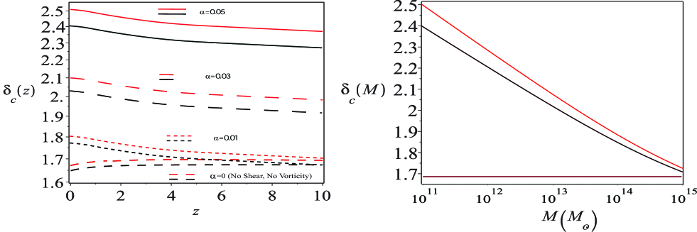
Figure 1: The threshold of collapse $\delta_{c}$, as function of redshift, and mass. In the left panel, $\delta_{c}$ vs redshift is plotted. The prediction for $\delta_{c}(z)$ for the $\Lambda$CDM model are represented by the red lines. The values of $\alpha$ varies from 0.05 (solid line) (galactic mass scale), to 0.03 (long dashed line), to 0.01 (dotted line) (cluster mass scale), and to 0 (dashed line). The right panel plots $\delta_{c}$ vs mass. The solid red line represents the result of the ESCM model, the red dashed line that of the elliptictal collapse model of (Sheth et al., 2001), and the brown line the $\Lambda$CDM expectation when no shear and rotation are taken into account.

The effect of shear (Hoffman, 1986, 1989; Zaroubi and Hoffman, 1993), and rotation (Del Popolo and Gambera, 1998, 1999, 2000; Del Popolo et al., 2001; Del Popolo, 2002a; Del Popolo et al., 2013b; Pace et al., 2019) on the collapse are manifold.

One general feature is that of slowing down the collapse (Peebles, 1990; Audit et al., 1997; Del Popolo et al., 2001; Del Popolo, 2002a). Mass function (Del Popolo and Gambera, 1999, 2000; Del Popolo et al., 2013b; Pace et al., 2014a; Mehrabi et al., 2017; Del Popolo et al., 2017; Pace et al., 2019), two-point correlation function, (Del Popolo et al., 2005), scaling relations like the mass-temperature, and luminosity-temperature relation (Del Popolo et al., 2005) (Del Popolo, 2002b; Del Popolo et al., 2019), are modified. This is connected to the change of the typical parameters of the SCM.

III.1 Threshold of collapse with shear, rotation, and dynamical friction

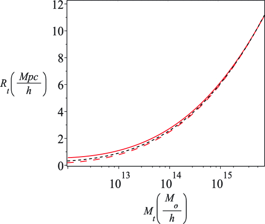
Figure 2: Turnaround radius $R_{\rm t}$ vs mass, $M_{\rm t}$. The solid red line represents the TAR predicted by the standard SCM, and the dashed red line ESCM result for the $\Lambda$CDM model. The black dotted line the result of the ESCM for the AS model.

Fig. 1 shows how shear, rotation, and dynamical friction (shortly SRD) change the collapse threshold, $\delta_{c}$. We show the dependence from redshift in the left panel, and mass in the right panel. The red line represents the predictions of the ESCM for $\delta_{c}(z)$ for the $\Lambda$CDM model, while the black line the ESCM in the case of one DE model, the Albrecht-Skordis (Albrecht and Skordis, 2000) (AS) (black line).

In the left panel, from top to bottom, the value of $\alpha$ varies from 0.05 (solid line) corresponding to a mass $\simeq 10^{11}M_{\odot}$, to 0.03 (long dashed line), corresponding to a mass $\simeq 10^{13}M_{\odot}$, to 0.01 (dotted line), corresponding to a mass $\simeq 10^{15}M_{\odot}$, and to 0 (dashed line). The value of $\delta_{c}(z)$ for $\alpha=0.05$, is $\simeq 30\%$ larger than in the $\alpha=0$ case.

In the case, of no shear, rotation ($\alpha=0$) and dynamical friction, $\delta_{c}$, has a weak dependence from redshift in the $z$ range $[0,2]$, and then assumes the value predicted by the Einstein de Sitter model.

In other terms, SRD gives rise to a non-flat threshold, $\delta_{c}$, which is monotonically decreasing with redshift. Moreover, the larger is $\alpha$, the larger is the difference between the values of $\delta_{c}(z)$, as shown by the different curves.

Of the DE quintessence models in literature, we plotted the AS model because the other models considered in previous papers (Pace et al., 2010; Del Popolo et al., 2013a) (INV1 ($w_{0}=-0.4$), INV2 ($w_{0}=-0.79$), 2EXP ($w_{0}=-1$), CNR ($w_{0}=-1$), CPL ($w_{0}=-1$), SUGRA ($w_{0}=-0.82$) (see (Pace et al., 2010; Del Popolo et al., 2013b))) are contained in the envelope between the region included in the $\Lambda$CDM and the AS model (see Fig. 4 of (Pace et al., 2010)).

The right panel of Fig. 1 plots $\delta_{c}(M)$ versus the mass. In absence of SRD the value of $\delta_{c}$ is constant (brown line). in presence of SRD, $\delta_{c}$ becomes mass dependent, and monotonically decreases with mass. This means that in order a less massive perturbations (e.g., galaxies) form structures must cross a higher threshold than more massive ones. This behavior, is related to the anticorrelation of the angular momentum acquired by the proto-structure and its height. Since low peaks acquire larger angular momentum than high peaks, they need a higher density contrast to collapse and form structures (Del Popolo and Gambera, 1998; Del Popolo et al., 2001; Del Popolo, 2002a, 2009; Ryden, 1988; Peebles, 1990; Audit et al., 1997).

As shown in the left and right panel of Fig. 1, the effect of dynamical friction is that of increasing the values of $\delta_{c}(z)$, and $\delta_{c}(M)$ with respect to the case it is not present as shown in (Del Popolo et al., 2020).

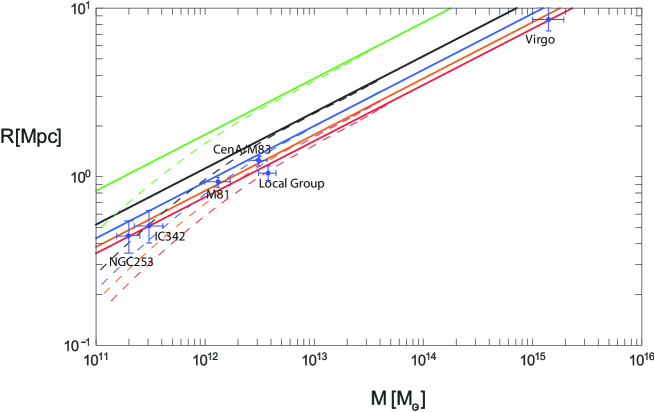
Figure 3: Stable structures mass-radius relation for different $w$. The solid lines from top to bottom represent $w=-0.5$ (solid green line), -1 (black solid line), -1.5 (blue solid line) ,-2 (pink solid line), -2.5 (red solid line). The results of the ESCM are represented by the dashed lines. The dots with error bars, are data as in (Pavlidou et al., 2014).

III.2 Comparison of TAR, in the $\Lambda$CDM, ESCM, and DE models

Shear, rotation, and dynamical friction modify the TAR. In order to show this, we may compare the predictions of the $\Lambda$CDM, that of the ESCM, and DE models. (Pavlidou and Tomaras, 2014) and (Pavlidou et al., 2014) calculated the maximum TAR, MTAR, that is, the radius of the surface where $\ddot{R}=0$. (Pavlidou et al., 2014) found

$$R_{\rm ta}=\left[\frac{-3M}{4\pi\rho_{\rm de}(1+3w)}\right]^{1/3}$$ (13)

which in the case of the $\Lambda$CDM model ($w=-1$) reduces to

$$R_{\rm ta}=\left[\frac{3GM}{\Lambda}\right]^{1/3}$$ (14)

(Pavlidou and Tomaras, 2014).

In their estimation, they assumed that shear and rotation were not present. Their expression can be generalized to the case shear, and rotation are non zero. This can be done using Eq. (6), obtaining

$$R_{\rm ta}=\left[\frac{-3M}{4\pi\rho_{\rm de}(1+3w)+(\sigma^{2}-\omega^{2})}\right]^{1/3}$$ (15)

In the paper, we will get and plot the TAR, not MTAR, since we compare with (Lopes et al., 2018), which calculated the TAR.

Fig. 2, shows the TAR predicted by the $\Lambda$CDM model (solid red line), that of the ESCM model (taking into account shear rotation, and dynamical friction) (red dashed line) for the $\Lambda$CDM model, and the AS model (black dashed line). When shear, rotation and dynamical friction are taken into account the collapse is slowed down, and the the TAR is smaller. The difference between the $\Lambda$CDM model, and the ESCM preditions increases going towards smaller masses. This is mainly related to the larger rotation of smaller objects, and reach a maximum difference of $\simeq 60\%$. The black dashed line, as already reported, is the AS model, which has a slightly larger TAR with

III.3 Constraints on DE EoS parameter

Table 1: The allowed ranges of $w$ based on the ESCM model.

Stable structure	range of $w$
M81	$w\geq-1.5$
IC342	$w\geq-1$
NGC253	$w\geq-1$
CenA/M83	$w\geq-1.5$
Local Group	$w\geq-2$
Virgo	$w\geq-2$

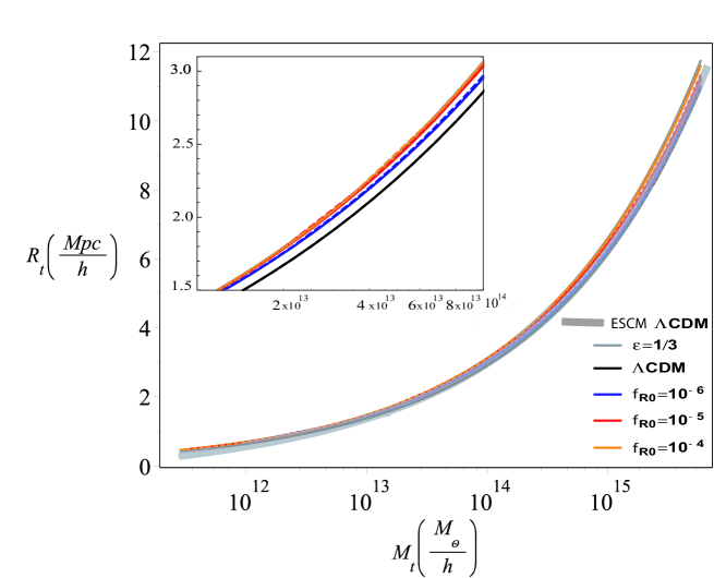
Figure 4: Turnaround radius, $R_{\rm t}$ vs mass, $M_{\rm t}$. The plot represents the result obtained by (Lopes et al., 2018) for $R_{\rm ta}$ vs mass for the $\Lambda$CDM model, the model with $\epsilon=1/3$, and $f(R)$ with $f_{\rm R0}=10^{-6}$, $10^{-5}$, and $10^{-4}$. The gray band represents our prediction for the $\Lambda$CDM model, obtained with the ESCM, with the 68% confidence level region.

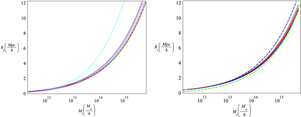
Figure 5: The turnaround radius, $R_{\rm t}$ vs mass, $M_{\rm t}$ obtained with the ESCM for the DE models. Left panel: from top to bottom, the cyan, blue, brown, magenta, black, red, and green lines represent the INV1, INV2, SUGRA, $w_{09}$, AS, $\Lambda$CDM without shear, and rotation, and $\Lambda$CDM with shear, and rotation, respectively. Right panel: the solid lines are the $\Lambda$CDM, and $f(R)$ models of (Lopes et al., 2018), while the blue dashed line, and the green dashed lines, are the INV2 model, and the $\Lambda$CDM with shear, rotation, and dynamical friction, plotted in the left panel.

Knowing the relation between TAR, the structure mass, and the EoS parameter, it is possible to obtain some constraints on the DE EoS ($w$). This was tried by (Pavlidou et al., 2014) by means of Eq. (13). In general, a great number of DE models are described through the equation of state parameter, $w(a)$. The last depends on its present value $w_{0}$, on that at matter-radiation equality epoch, and some other parameters at the same epoch (see Eq. 23 of (Pace et al., 2010)). If one wants to constrain the EoS parameter, $w$ evolution, high redshift structures are needed. If by converse, one wants to constrain the values of $w_{0}$ small $z$ cosmic structures may be used. (Pavlidou et al., 2014) compared the predicted TAR at different $w$ in the plane $M_{t}$-$R_{t}$, finding constraints on $w_{0}$. To this aim data from several structures (e.g., Milky Way (MW), M81/M82 group, Local Group, Virgo cluster, Fornax-Eridanus group) were used. It is of fundamental importance to note, that the constrain depends from the model used. As shown by (Peirani and de Freitas Pacheco, 2008), the mass of the structure, and its TAR changes when to the standard SCM (considering only the gravitational potential) is also added the cosmological constant (Eq. 1 of (Peirani and de Freitas Pacheco, 2008)). This was also pointed out comparing the values predicted by several Karachentsev’s paper (e.g., (Karachentsev et al., 2002; Karachentsev, 2005), for M81, the local group, and neighboring groups) with those of (Peirani and de Freitas Pacheco, 2008).

In Fig. 3, the solid lines obtained from the equation of TAR (Eq. 13), correspond to $w=-2.5$, -2, -1.5, -1, -0.5, from bottom to top when shear, rotation, and dynamical friction are absent. The dashed lines are the corrections obtained when shear, rotation, and dynamical friction are taken into account. The range of $w$ for which no stable structures exist is given by the parameter space above each line. (Pavlidou et al., 2014) discussed some constraints to $w$, based on the highest mass objects. As shown by the dashed lines, one has to expect that at masses smaller than $10^{13}M_{\odot}$ the TAR is modified by the presence of shear, rotation, and dynamical friction. As a consequence, structures at smaller masses can give different constraints to $w$. At the same time, following (Peirani and de Freitas Pacheco, 2008), taking also the effect of dynamical friction, we see that the constraints on the cosmic structure studied, and plotted in Fig. 3, is noteworthy different from that of (Del Popolo et al., 2020). The values of TAR and mass for each of the objects in Fig. 3 were obtained using the SCM with dynamical friction, and using a method described by (Peirani and de Freitas Pacheco, 2006, 2008) (see Appendix). In Table 1, we report the constraints we obtained.

III.4 Comparison with TAR in $f(R)$ theories

In this section, we compare the evolution of the TAR in the ESCM, and the $f(R)$ theories. The evolution of TAR in General Relativity (GR), and in the $f(R)$ theories was investigated by (Lopes et al., 2018). Modified Gravity (MG) effects were introduced in the equation of the evolution of overdensity (their Eq. 3.3) by means of the parameter $\epsilon(a,k)$, where $k$ is the (angular) wavenumber. GR is recovered when $\epsilon(a,k)$ is zero, and our Eq. (5), is recovered in the case $\epsilon(a,k)$ is zero, and shear, and rotation are put equal to zero. In other terms, our Eq. (5) is a generalization of Eq. 3.3 of (Lopes et al., 2018), for the case $\epsilon(a,k)$ is zero. Consequantly, their Figs. 1, 3, similarly to the left panel of our Fig. 1, and to the $\Lambda$CDM, and DE models without shear, and rotation, as shown in (Pace et al., 2010), shows a monotonic increase of $\delta_{c}(z)$. Their Fig. 4 shows an almost flat behavior of $\delta_{c}(M)$, with variations from constancy of the order of 1%. The behavior of $\delta_{c}(z)$, and $\delta_{c}(M)$ in (Lopes et al., 2018) disagrees with the prediction of several papers (e.g., (Sheth et al., 2001; Del Popolo et al., 2013a, b; Pace et al., 2014a; Mehrabi et al., 2017; Del Popolo et al., 2017)). The previous papers showed that in order to have a mass function reproducing simulations, the threshold must be a monotonic decreasing function of mass. Since in (Lopes et al., 2018) $\delta_{c}(M)$ is practically constant, and $\delta_{c}(z)$ is a monotonic increasing function of redshift, this implies that (Lopes et al., 2018) results cannot reproduce the mass function obtained in simulations, and observations. This is due to the the fact (Lopes et al., 2018) discarded the effect of shear, and rotation, and in general of aspericities. A more detailed discussion of this aspect can be found in (Del Popolo et al., 2020).

Going back to our main goal, namely the use of the TAR to disentangle between GR and MG, and GR and DE models, discussed by several authors (e.g., (Lopes et al., 2018)), we will compare (Lopes et al., 2018) prediction on the $M_{t}$-$R_{t}$ relation with that of our ESCM. In Fig. 4, the result obtained by (Lopes et al., 2018) for $R_{\rm t}$ vs mass for the $\Lambda$CDM model, the model with $\epsilon=1/3$, and $f(R)$ with $f_{\rm R0}=10^{-6}$, $10^{-5}$, and $10^{-4}$, are plotted. Our prediction for the $\Lambda$CDM model, obtained with the ESCM, with the 68% confidence level region, are represented by the grey band. The 68% confidence level was obtained, as in (Del Popolo et al., 2020), by means of a Monte Carlo simulation. The result of the plot is slightly different from Fig. 4 of (Del Popolo et al., 2020). Because of the presence of dynamical friction, which further contribute to slow down the collapse, the TAR has smaller values. Consequently, the TAR in the ESCM model does not completely overlap with that of (Lopes et al., 2018), as happened in (Del Popolo et al., 2020). This means that the study of the top values of the $M_{t}$-$R_{t}$ relation could disentangle the GR predictions from that of the $f(R)$ theories. Choosing peculiar values of the TAR would be possible to disentangle between GR, and $f(R)$ theories.

The predictions of some of the quintessence DE models previously cited are compared in Fig. 5 to the same $f(R)$ models of (Lopes et al., 2018) plotted in Fig. 4. All the curves are obtained by means of the ESCM applied to the DE models of the TAR. From top to bottom, the cyan, blue, brown, magenta, black, red, and green lines represent the INV1, INV2, SUGRA, $w_{09}$, AS, $\Lambda$CDM without shear, and rotation, and $\Lambda$CDM with shear, and rotation, respectively.

The comparison of the (Lopes et al., 2018) predictions for TAR with that of the DE models are plotted in the right panel. In this plot, we show only INV2 (blue dashed line), and the $\Lambda$CDM with shear, rotation, and dynamical friction (green dashed line). With exception of INV1, the two quoted curves contain all other DE models.

The other lines are the $\Lambda$CDM, and $f(R)$ models of (Lopes et al., 2018). Differently from Fig. 4, the DE models contain the (Lopes et al., 2018) prediction for TAR. As a consequence the TAR cannot be used to disentangle DE, and $f(R)$ theories predictions.

IV Conclusions

In this paper, we discussed how shear, rotation, and dynamical friction change the TAR, and some of the parameters of the SCM. The results were obtained using an ESCM taking into account the effects of shear, vorticity, and dynamical friction, to determine the $R_{\rm t}-M_{\rm t}$, in $\Lambda$CDM, and in DE scenarios. We extended numerically the formula for maximum TAR obtained in (Del Popolo et al., 2020), to take into account dynamical friction. The value of TAR is reduced by shear, rotation, and dynamical friction, especially at galactic scales. Using the $R_{\rm t}-M_{\rm t}$ relationship, and data from stable structures, one can obtain constraints to $w$. Its values are smaller for structures with masses approximately smaller that $10^{13}M_{\odot}$. In this paper, we recalculated the mass, and TAR of M81/M82 group, Local Group, Virgo cluster, NGC253, IC342, CenA/M83 group following (Peirani and de Freitas Pacheco, 2006, 2008).

A comparison of the $R_{\rm t}-M_{\rm t}$ relationship obtained for $\Lambda$CDM, and DE scenarios with (Lopes et al., 2018) prediction of the $f(R)$ theories, shows that $R_{\rm t}-M_{\rm t}$ relationship in the $f(R)$ models are practically identical to that of of DE scenarios. This implies that the $R_{\rm t}-M_{\rm t}$ relationship is not a good probe to disentangle between GR, and DE models predictions. The situation is different in the case of the $\Lambda$CDM model. In this case, the 68% confidence level region does not overlap with that of the $f(R)$ models. The higher values of the TAR could be used to disentangle between $f(R)$ theories, and GR.

Appendix A Mass and TAR of structures

The most general equation taking account of shear, rotation, and dynamical friction is Eq. (12). We will rewrite it in adimensional form. Assuming that $J=kR^{\alpha}$, with $\alpha=1$, in agreement with (Bullock et al., 2001), and $k$ constant. In terms of the variables $y=R/R_{0}$, $t=x/H_{0}$, Eq. (12) can be written as

$$\frac{d^{2}y}{dx^{2}}=-\frac{A}{2y^{2}}+\Omega_{\Lambda}y+\frac{K_{j}}{y}-\frac{\eta}{H_{0}}\frac{dy}{dx},$$ (16)

where $K_{j}=k\frac{1}{(H_{0}R_{0})^{2}}$, $A=\frac{2GM}{H_{0}^{2}R_{0}^{3}}$, and

$$H=H_{0}\sqrt{\left(\frac{a_{0}}{a}\right)^{3}\Omega_{m}+\Omega_{\Lambda}}.$$ (17)

Eq.(16) has a first integral, given by

$$u^{2}=\left(\frac{dy}{dx}\right)^{2}$$

$$=\frac{A}{y}+\Omega_{\Lambda}y^{2}+2K_{j}\log{y}-2\frac{\eta}{H_{0}}\int\left(\frac{dy}{dx}\right)^{2}dx+K$$ (18)

where $K=\frac{2E}{(H_{0}R_{0})^{2}}$, and $E$ is the energy per unit mass of a shell.

The previous equation can solved as described in (Peirani and de Freitas Pacheco, 2006, 2008).

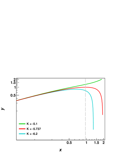
Figure 6: Evolution of shell radius for different values of $K$. The red, cyan, and green lines correspond to $K=-5.737$, $K=-6.2$, and $K=-5.1$, respectively.

The mass, and turn-around radius of some groups of galaxies, is obtained finding a relation between the velocity, and radius, $v-R$. The last will be fitted to the data. The $v-R$ relation is obtained as follows. Let’s consider Fig.6. This is a solution of Eq. (12) for different values of $K$. The vertical line corresponds to $x=0.964$. Its intersection with the curves, solution of Eq. (12) (cyan, red, green) gives, for each one a value $y(x)=y(0.964)$. The solution of Eq. (12), also gives the velocity, allowing us to find $u(x)=u(0.964)$. We will get a couple of value $(y,u)$ for each intersection of the vertical line with the curves. This allows us to find a series of points that can be fitted with a relation of the form $u=-b/y^{n}+by$ obtaining $u=-1.3436/y^{0.9107}+1.3436y$. This last relation can be written in physical units as follows.

$$v(R)=-bH_{0}R_{0}\left(\frac{R_{0}}{R}\right)^{n}+bH_{0}R$$ (19)

. Substituting in this equation, $R_{0}=(\frac{2GM}{H_{0}^{2}})^{\frac{1}{3}}$, we get

$$v(R)=-b\frac{H_{0}}{R^{n}}\left(\frac{2GM}{AH_{0}^{2}}\right)^{\frac{n+1}{3}}+bH_{0}R$$ (20)

or

$$v(R)=-\frac{-0.66385H_{0}}{R^{n}}\left(\frac{GM}{H_{0}^{2}}\right)^{\frac{n+1}{3}}+1.3436H_{0}R$$ (21)

where $n=0.9107$. Eq. (21) satisfy the condition $v(R_{0})=0$. Fitting the equation to the data of (Peirani and de Freitas Pacheco, 2006) (Fig. 2), and (Peirani and de Freitas Pacheco, 2008) (Fig. 2) one obtains the value of the Hubble parameter , $H_{0}$, and TAR. Solving Eq. (12) one can obtain the value of $A$, and solving the equation $A=\frac{2GM}{H_{0}^{2}R_{0}^{3}}$, being $H_{0}$, and $R_{0}$, one gets the mass, $M$.

References

- Sanders (2010) R. H. Sanders, The Dark Matter Problem: A Historical Perspective (Cambridge University Press, 2010).
- Profumo (2017) S. Profumo, An Introduction to Particle Dark Matter (World Scientific, 2017).
- Li et al. (2011) M. Li, X.-D. Li, S. Wang, and Y. Wang, Communications in Theoretical Physics 56, 525 (2011), arXiv:1103.5870 .
- Del Popolo (2013) A. Del Popolo, in AIP Conf. Proc., Vol. 1548 (2013) pp. 2–63.
- Ade (2016) P. A. R. e. a. Ade, Astron. Astrophys. 594, A13 (2016).
- de Blok (2010) W. J. G. de Blok, Advances in Astronomy 2010, 789293 (2010), arXiv:0910.3538 .
- Moore et al. (1999) B. Moore, S. Ghigna, F. Governato, G. Lake, and T. Quinn, Astrophys. J. 524, L19 (1999).
- McGaugh (2004) S. S. McGaugh, Astrophys. J. 609, 652 (2004).
- McGaugh et al. (2016) S. S. McGaugh, F. Lelli, and J. M. Schombert, Phys. Rev. Lett. 117, 201101 (2016).
- Aprile (2017) E. e. a. Aprile, Phys. Rev. Lett. 119, 181301 (2017).
- Abecrcrombie (2020) D. e. a. Abecrcrombie, Physics of Dark Universe 27, 100371 (2020).
- Ackermann (2015) M. e. a. Ackermann, Phys. Rev. Lett. 115, 231301 (2015).
- Chan and Leung (2017) M. H. Chan and C. H. Leung, Scientific Reports 7, 14895 (2017), arXiv:1710.08123 .
- Chan et al. (2019) M. H. Chan, L. Cui, J. Liu, and C. S. Leung, ApJ 872, 177 (2019), arXiv:1901.04638 .
- Chan and Lee (2020) M. H. Chan and C. M. Lee, Phys. Rev. D (2020).
- Weinberg (1989) S. Weinberg, Reviews of Modern Physics 61, 1 (1989).
- Velten et al. (2014) H. E. S. Velten, R. F. vom Marttens, and W. Zimdahl, European Physical Journal C 74, 3160 (2014), arXiv:1410.2509 .
- Copeland et al. (2006) E. J. Copeland, M. Sami, and S. Tsujikawa, International Journal of Modern Physics D 15, 1753 (2006), arXiv:hep-th/0603057 .
- Horndeski (1974) G. W. Horndeski, International Journal of Theoretical Physics 10, 363 (1974).
- Milgrom (1983) M. Milgrom, ApJ 270, 365 (1983).
- Zwiebach (1985) B. Zwiebach, Physics Letters B 156, 315 (1985).
- Moffat (2006) J. W. Moffat, JCAP 3, 004 (2006), gr-qc/0506021 .
- Nojiri et al. (2005) S. Nojiri, S. D. Odintsov, and M. Sasaki, Phys. Rev. D 71, 123509 (2005), hep-th/0504052 .
- Bekenstein (2010) J. D. Bekenstein, “Modified gravity as an alternative to dark matter,” in Particle Dark Matter : Observations, Models and Searches, edited by G. Bertone (Cambridge University Press, 2010) p. 99.
- De Felice and Tsujikawa (2010) A. De Felice and S. Tsujikawa, Living Reviews in Relativity 13, 3 (2010), arXiv:1002.4928 .
- Linder (2010) E. V. Linder, Phys. Rev. D 81, 127301 (2010), arXiv:1005.3039 .
- Milgrom (2014) M. Milgrom, Phys. Rev. D 89, 024027 (2014), arXiv:1308.5388 .
- Lovelock (1971) D. Lovelock, Journal of Mathematical Physics 12, 498 (1971).
- Hořava (2009) P. Hořava, Phys. Rev. D 79, 084008 (2009), arXiv:0901.3775 .
- Rodríguez and Navarro (2017) Y. Rodríguez and A. A. Navarro, in Journal of Physics Conference Series, Journal of Physics Conference Series, Vol. 831 (2017) p. 012004, arXiv:1703.01884 .
- Deffayet et al. (2010) C. Deffayet, O. Pujolàs, I. Sawicki, and A. Vikman, JCAP 10, 026 (2010), arXiv:1008.0048 .
- Verlinde (2017) E. P. Verlinde, SciPost Physics 2, 016 (2017).
- Buchdahl (1970) H. A. Buchdahl, MNRAS 150, 1 (1970).
- Bhattacharya et al. (2017) S. Bhattacharya, K. F. Dialektopoulos, A. Enea Romano, C. Skordis, and T. N. Tomaras, JCAP 7, 018 (2017), arXiv:1611.05055 .
- Lopes et al. (2018) R. C. C. Lopes, R. Voivodic, L. R. Abramo, and J. Sodré, Laerte, JCAP 2018, 010 (2018), arXiv:1805.09918 .
- Lopes et al. (2019) R. C. C. Lopes, R. Voivodic, L. R. Abramo, and J. Sodré, Laerte, JCAP 2019, 026 (2019), arXiv:1809.10321 .