Adaptive Learning in Continuous Games:
Optimal Regret Bounds and Convergence to Nash Equilibrium

Abstract

In game-theoretic learning, several agents are simultaneously following their individual interests, so the environment is non-stationary from each player’s perspective. In this context, the performance of a learning algorithm is often measured by its regret. However, no-regret algorithms are not created equal in terms of game-theoretic guarantees: depending on how they are tuned, some of them may drive the system to an equilibrium, while others could produce cyclic, chaotic, or otherwise divergent trajectories. To account for this, we propose a range of no-regret policies based on optimistic mirror descent, with the following desirable properties: it n) they do not require any prior tuning or knowledge of the game; it n) they all achieve $\operatorname{\mathcal{O}}(\sqrt{T})$ regret against arbitrary, adversarial opponents; and it n) they converge to the best response against convergent opponents. Also, if employed by all players, then it n) they guarantee $\operatorname{\mathcal{O}}(1)$ social regret; while it n) the induced sequence of play converges to Nash equilibrium with $\operatorname{\mathcal{O}}(1)$ individual regret in all variationally stable games (a class of games that includes all monotone and convex-concave zero-sum games).

1 Introduction

A fundamental problem at the interface of game theory and online learning concerns the exact interplay between static and dynamic solution concepts. On the one hand, if all players know the game and are assumed to be rational, the most relevant solution concept is that of a Nash equilibrium: this represents a stationary state from which no player has an incentive to deviate. On the other hand, this knowledge is often unavailable, so players must adapt to each other’s actions in a dynamic manner; in this case, the standard figure of merit is an agent’s regret, i.e., the cumulative difference in performance between an agent’s trajectory of play and the best action in hindsight. Optimistically, one would expect that the two approaches should yield compatible answers – and, indeed, one direction is clear: Nash equilibrium never incurs any regret. Our paper deals with the converse question, namely: Does no-regret lead to Nash equilibrium?

This question has attracted considerable interest in the literature and the answer can be particularly nuanced. To provide some context, it is well known that the empirical frequency of no-regret play in finite games converges to the set of coarse correlated equilibria (CCE) – also known as the game’s Hannan set [18, 19]. This is sometimes interpreted as a “universal equilibrium convergence” result, but one needs to keep in mind that itn) the type of convergence involved is not the actual, day-to-day play but the empirical frequency of play; and itn) the game’s coarse correlated equilibria set may contain elements that fail even the most basic rationalizability axioms. In particular, Viossat and Zapechelnyuk [46] constructed a simple two-player game (a variant of rock-paper-scissors with a feeble twin) that admits CCE supported exclusively on strictly dominated strategies.

This interplay becomes even more involved because the behavior of a no-regret learning algorithm could switch from convergent to non-convergent by a slight variation of its hyperparameters or a small perturbation of the game. As a simple example, optimistic gradient methods are known to converge to Nash equilibrium in smooth convex-concave games, provided that they are tuned appropriately. However, if the algorithm’s step-size is out-of-tune even by a little bit, the trajectory of play could diverge and the players’ mean behavior could converge to an irrelevant off-equilibrium profile (we provide a concrete example of this behavior in Section 3). Equally pernicious examples can be found in symmetric $2\times 2$ congestion games: even though such games have a very simple equilibrium structure (a unique, evolutionarily stable equilibrium), running a no-regret learning algorithm – like the popular multiplicative weights update scheme – may lead to chaos [40, 10, 11].

Our contributions and related work.

In view of all this, the equilibrium convergence properties of no-regret learning depend crucially on the algorithm’s tuning – and the parameters required for this tuning could be beyond the players’ reach. With this in mind, we propose a range of no-regret policies with the following desirable properties:

1. They do not require any prior tuning or knowledge of the game’s parameters: each player updates their individual step-size with purely local, individual gradient information.

2. They guarantee an order-optimal $\operatorname{\mathcal{O}}(\sqrt{T})$ regret bound against adversarial play, and they further enjoy constant social regret when all players employ one of these algorithms.

3. In any continuous game with smooth, convex losses, the sequence of chosen actions of any player converges to best response against convergent opponents.

4. If all players follow one of these algorithms, the induced trajectory of play converges to Nash equilibrium and the individual regret of each player is bounded as $\operatorname{\mathcal{O}}(1)$ in all variationally stable games – a large class of games that contains as special cases all convex-concave zero-sum games and monotone / diagonally convex games.

To the best of our knowledge, the proposed methods – optimistic dual averaging (OptDA) and dual stabilized optimistic mirror descent (DS-OptMD) – are the first in the literature that concurrently enjoy even a subset of these properties in games with continuous action spaces. To achieve this, they rely on two principal ingredients: itn) a regularization mechanism as in the popular “follow the regularized leader” (FTRL) class of policies [44, 6]; and itn) a player-specific adaptive step-size rule inspired by [42]. In this regard, they resemble the policy employed by Syrgkanis et al. [45] who established comparable individual/social regret guarantees for finite games. Our results extend the analysis of Syrgkanis et al. [45] to games with continuous – and possibly unbounded – action spaces, and, as a pleasing after-effect, they also shave off all logarithmic factors.

Concerning the convergence behavior of optimistic mirror descent (OptMD), it is known that the sequence of realized actions converges to a Nash equilibrium in all variationally stable games, provided that every player runs the algorithm with a sufficiently large regularization parameter, common across all players [35, 21]. This result cannot be attained by “vanilla” first-order methods that do not include an extra-gradient mechanism, but it also comes with several important caveats. First, running OptMD with a constant step-size robs the algorithm of any fallback guarantees: a player’s individual regret may grow linearly if the other players switch to an adversarial behavior (e.g., as part of a “grim trigger” strategy). Second, the method’s convergence is contingent on the players’ using a fine-tuned regularization parameter, depending on the smoothness modulus of their payoff functions. This constant cannot be estimated without prior, global knowledge of the game’s primitives, and if a player misestimates it, the algorithm’s convergence breaks down completely (see Fig. 1 in Section 3).

In terms of trajectory convergence of adaptive methods, the closest antecedents of our results are the recent papers by Lin et al. [29] and Antonakopoulos et al. [2, 3], where the authors propose an adaptive step-size rule for cocoercive games and variational inequalities respectively. However, in both cases, the method’s step-size requires global gradient information, and therefore does not apply to a fully distributed game-theoretic setting.

2 Online learning in games

In this section, we present the necessary background material on normal form games with continuous action spaces and the corresponding learning framework.

2.1 Games with continuous action spaces

Definitions and examples.

Throughout the paper, we focus on normal form games played by a finite set of players $\mathcal{N}\coloneqq\{1,\ldots,N\}$. Each player $i\in\mathcal{N}$ is associated with a closed convex action set ${\mathcal{X}^{i}}\subseteq\mathbb{R}^{d_{i}}$ and a loss function ${\ell^{i}}\colon\mathcal{X}\to\mathbb{R}$, where $\mathcal{X}\coloneqq\prod_{i=1}^{N}{\mathcal{X}^{i}}$ denotes the game’s joint action space. For the sake of clarity, a joint action of multiple players will be typeset in bold; in particular, the joint action profile of all players will be written as $\mathbf{x}=({x^{i}},{\mathbf{x}^{-i}})=({x^{i}})_{i\in\mathcal{N}}$, where ${x^{i}}$ and ${\mathbf{x}^{-i}}$ respectively denote the action of player $i$ and the joint action of all players except player $i$.

Our blanket assumption concerning the players’ loss functions is the following:

Assumption 1 (Individual convexity + Smoothness).

For each $i\in\mathcal{N}$, ${\ell^{i}}$ is continuous in $\mathbf{x}$ and convex in ${x^{i}}$ –  that is, ${\ell^{i}}(\cdot,{\mathbf{x}^{-i}})$ is convex for all ${\mathbf{x}^{-i}}\in\prod_{j\neq i}{\mathcal{X}^{j}}$. Furthermore, the subdifferential $\partial_{i}{\ell^{i}}$ of ${\ell^{i}}$ relative to ${x^{i}}$ admits a Lipschitz continuous selection ${V^{i}}$ on $\mathcal{X}$.

In the sequel, we will refer to any game that satisfies Assumption 1 as a (continuous) convex game. For the sake of concreteness, we briefly discuss below two examples of such games.

Example 1 (Mixed extensions of finite games).

In a finite game, each player $i\in\mathcal{N}$ has a finite set ${\mathcal{A}^{i}}$ of pure strategies and no assumptions are made on the loss function ${\ell^{i}}\colon\prod_{i=1}^{N}{\mathcal{A}^{i}}\to\mathbb{R}$. A mixed strategy for player $i$ is a probability distribution ${x^{i}}$ over their pure strategies, so the player plays $k$ with probability ${x_{k}^{i}}$ (i.e., the $k$-th coordinate of ${x^{i}}$). In this case, ${\mathcal{X}^{i}}=\operatorname{\Delta}({\mathcal{A}^{i}})$ is the set of mixed strategies, the expected loss at a mixed profile is given by ${\ell^{i}}(\mathbf{x})=\operatorname{\mathbb{E}}_{\mathbf{s}\sim\mathbf{x}}{{\ell^{i}}(\mathbf{s})}$, and the player’s feedback is the observation of the expected loss $\operatorname{\mathbb{E}}_{{\mathbf{s}^{-i}}\sim{\mathbf{x}^{-i}}}[{\ell^{i}}(k,{\mathbf{s}^{-i}})]$ for all $k\in{\mathcal{A}^{i}}$. Our blanket assumption holds trivially since the mixed losses are multilinear.

Example 2 (Kelly auctions).

Consider an auction of $K$ splittable resources among $N$ bidders (players). For the $k$-th resource, let $q_{k}$ and $c_{k}$ denote respectively its available quantity and the entry barrier for bidding on it; for the $i$-th bidder, let ${b^{i}}$ and ${\textsl{g}^{i}}$ denote respectively the bidder’s budget and marginal gain from obtaining a unit of resources. During play, each bidder submits a bid ${x_{k}^{i}}$ for each resource $k$ with the constraint $\sum_{k=1}^{K}{x_{k}^{i}}\leq{b^{i}}$. Resources are then allocated to bidders proportionally to their bids, so the $i$-th player gets ${\rho_{k}^{i}}=q_{k}{x_{k}^{i}}/(c_{k}+\sum_{i=1}^{N}{x_{k}^{i}})$ units of the $k$-th resource. The utility of player $i\in\mathcal{N}$ is given by ${u^{i}}(\mathbf{x})=\sum_{k=1}^{K}({\textsl{g}^{i}}{\rho_{k}^{i}}-{x_{k}^{i}})$, and the loss function is ${\ell^{i}}=-{u^{i}}$.

Nash equilibrium.

In terms of solution concepts, the most widely used notion is that of a Nash equilibrium, i.e., a strategy profile from which no player has incentive to deviate unilaterally. Formally, a point $\mathbf{x_{\star}}\in\mathcal{X}$ is a Nash equilibrium if for all $i\in\mathcal{N}$ and all ${x^{i}}\in{\mathcal{X}^{i}}$, ${\ell^{i}}({x_{\star}^{i}},{\mathbf{x}_{\star}^{-i}})\leq{\ell^{i}}({x^{i}},{\mathbf{x}_{\star}^{-i}})$. For posterity, we will write $\mathcal{X}_{\star}$ for the set of Nash equilibria of the game; by a famous theorem of Debreu [15], $\mathcal{X}_{\star}$ is always nonempty if $\mathcal{X}$ is compact.

2.2 Regret minimization

In the multi-agent learning model that we consider, players interact with each other repeatedly via a continuous convex game. In more detail, during each round $t$ of the process, each player $i$ selects an action ${x^{i}_{t}}$ from their action set ${\mathcal{X}^{i}}$ and suffers a loss ${\ell^{i}}(\mathbf{x}_{t})$, where $\mathbf{x}_{t}=({x^{i}_{t}})_{i\in\mathcal{N}}$ is the joint action profile of all players. At the end of each round, the players receive as feedback a subgradient vector

$${g^{i}_{t}}={V^{i}}(\mathbf{x}_{t})\in\partial_{i}{\ell^{i}}({x^{i}_{t}},{\mathbf{x}^{-i}_{t}}),$$ (1)

and the process repeats. We will also write $\mathbf{V}=({V^{i}})_{i\in\mathcal{N}}$ for the joint feedback operator.

In this low-information setting, the players have no knowledge about the rules of the game, and can only improve their performance by “learning through play”. It is therefore unrealistic to assume that players can pre-compute their component of an equilibrium profile; however, it is plausible to expect that rational players would always seek to minimize their accumulated losses. This criterion can be quantified via each player’s individual regret, i.e., the difference between the player’s cumulative loss and the best they could have achieved by playing a given action from a compact comparator set ${\mathcal{P}^{i}}\subseteq{\mathcal{X}^{i}}$.

Following Shalev-Shwartz [44], we define the regret relative to a set of competing actions as

$${\operatorname{Reg}^{i}_{T}}({\mathcal{P}^{i}})=\max_{{p^{i}}\in{\mathcal{P}^{i}}}\sum_{t=1}^{T}\left({\ell^{i}}({x^{i}_{t}},{\mathbf{x}^{-i}_{t}})-{\ell^{i}}({p^{i}},{\mathbf{x}^{-i}_{t}})\right).$$

Likewise, for $\mathcal{P}\coloneqq\prod_{i=1}^{N}{\mathcal{P}^{i}}\subseteq\mathcal{X}$, we define the social regret by aggregating over all players, viz,

$$\operatorname{Reg}_{T}(\mathcal{P})=\sum_{i=1}^{N}{\operatorname{Reg}^{i}_{T}}({\mathcal{P}^{i}})=\max_{\mathbf{p}\in\mathcal{P}}\sum_{i=1}^{N}\sum_{t=1}^{T}\left({\ell^{i}}({x^{i}_{t}},{\mathbf{x}^{-i}_{t}})-{\ell^{i}}({p^{i}},{\mathbf{x}^{-i}_{t}})\right).$$

In this context, a sequence of play ${\mathbf{x}^{i}_{t}}$ of player $i$ incurs no individual regret if ${\operatorname{Reg}^{i}_{T}}({\mathcal{P}^{i}})=\operatorname{\mathnormal{o}}(T)$ for every (compact) set of alternative strategies; correspondingly, $\mathbf{x}_{t}$ incurs no social regret if $\operatorname{Reg}_{T}(\mathcal{P})=o(T)$.

In certain classes of games, the growth rate of the social regret can be related to the empirical mean of the players’ social welfare [45]. However, beyond this “aggregate” criterion, having no regret does not translate into any tangible guarantees for the quality of “day-to-day” play [46]. On that account, we will measure the optimality of ${x^{i}_{t}}$ at a given stage $t$ by the gap function

$${\operatorname{\Delta}_{{\mathcal{P}^{i}}}^{i}}(\mathbf{x}_{t})={\ell^{i}}({x^{i}_{t}},{\mathbf{x}^{-i}_{t}})-\min_{{p^{i}}\in{\mathcal{P}^{i}}}{\ell^{i}}({p^{i}},{\mathbf{x}^{-i}_{t}}),$$

i.e., the best that the player could have gained by switching to any other strategy in ${\mathcal{P}^{i}}$ at round $t$. When ${\mathcal{P}^{i}}={\mathcal{X}^{i}}$ and ${\operatorname{\Delta}_{{\mathcal{X}^{i}}}^{i}}(\mathbf{x}_{t})\leq\varepsilon$ for every $i\in\mathcal{N}$, we recover the definition of an $\varepsilon$-equilibrium.

3 Optimistic mirror descent and its failures

The OptMD template.

Our focal point in the sequel will be the optimistic mirror descent (OptMD) class of algorithms, which, under different assumptions, has been shown to enjoy optimal regret minimization guarantees [9, 41, 42]. To define it, assume that each player $i\in\mathcal{N}$ is equipped with a regularizer ${h^{i}}\colon{\mathcal{X}^{i}}\to\mathbb{R}$, i.e., a continuous, strongly convex function whose subdifferential $\partial{h^{i}}$ admits a continuous selection $\operatorname{\nabla}{h^{i}}$. Then, given a sequence of feedback signals $({g^{i}_{t}})_{t\in\mathbb{N}}$ (defined in (1) with the notation ${g^{i}_{0}}=0$), the $i$-th player plays an action ${x^{i}_{t}}={X^{i}_{t+\frac{1}{2}}}$ via the update rule

$${X^{i}_{t}}=\operatorname*{arg\,min}_{x\in{\mathcal{X}^{i}}}\thinspace\langle{g^{i}_{t-1}},x\rangle+{\lambda^{i}_{t-1}}{D^{i}}(x,{X^{i}_{t-1}}),~{}~{}~{}{X^{i}_{t+\frac{1}{2}}}=\operatorname*{arg\,min}_{x\in{\mathcal{X}^{i}}}\thinspace\langle{g^{i}_{t-1}},x\rangle+{\lambda^{i}_{t}}{D^{i}}(x,{X^{i}_{t}}),~{}~{}~{}$$ (OptMD)

where

$${D^{i}}(p,x)={h^{i}}(p)-{h^{i}}(x)-\langle\operatorname{\nabla}{h^{i}}(x),p-x\rangle\qquad p\in{\mathcal{X}^{i}},x\in\operatorname{dom}\partial{h^{i}},$$

denotes the Bregman divergence of ${h^{i}}$ and ${\lambda^{i}_{t}}$ is a player-specific regularization parameter (more details on this below). We also stress that, although (OptMD) produces two iterates per step, only one is actually played and directly contributes to the received feedback – namely, ${g^{i}_{t}}={V^{i}}({X^{i}_{t+\frac{1}{2}}},{\mathbf{x}^{-i}_{t}})$.

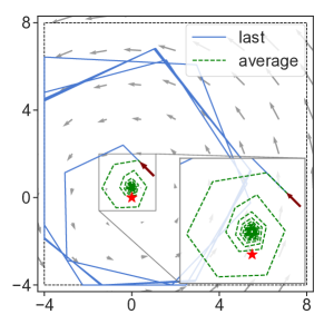
Figure 1: The trajectories of play and its time-average when running PEG for $\min_{\theta\in[-4,8]}\max_{\phi\in[-4,8]}\theta\phi$ with constant stepsize $\eta=0.7>1/\sqrt{3}$. Neither of the two converges to the unique Nash equilibrium at $(0,0)$.

Two of the most widely used instances of (OptMD) are the past extra-gradient (PEG) and optimistic multiplicative weights update (OMWU) algorithms, obtained respectively by the quadratic regularizer ${h^{i}}(x)=\lVert x\rVert_{2}^{2}/2$ and the negentropy function ${h^{i}}(x)=\sum_{k=1}^{d_{i}}x_{k}\log x_{k}$. For a detailed discussion, see [42, 31, 17, 20, 13] and references therein.

Failures of OptMD.

As we mentioned in the introduction, the convergence of (OptMD) is only guaranteed as long as the players’ regularization parameter ${\lambda^{i}_{t}}$ has been suitably fine-tuned – specifically, as long as it is sufficiently large relative to the smoothness modulus of the players’ loss functions. However, this tuning is contingent on a degree of coordination and global knowledge of the game that is often impractical: if ${\lambda^{i}_{t}}$ is not chosen properly, (OptMD) may – and, in fact, does – fail to converge.

We illustrate this failure in the simple min-max game ${\ell^{1}}(\theta,\phi)=\theta\phi=-{\ell^{2}}(\theta,\phi)$. In this case, if both players run the past extra-gradient (PEG) instance of (OptMD) with $\lambda>\sqrt{3}$, the sequence of play converges to the game’s unique Nash equilibrium. However, if the players misestimate the critical value $\sqrt{3}$ and choose $\lambda<\sqrt{3}$, the method no longer converges to equilibrium, in either the “ergodic” or “trajectory/last-iterate” sense (for a proof, see e.g., [48]). Moreover, as we show in Fig. 1, this “off-equilibrium” behavior persists even if we restrict the players’ actions to a compact set: in fact, not only does the method fail to converge to equilibrium, its average actually converges to an irrelevant action profile (an artifact of the trajectory’s divergence). This makes such failures particularly spurious and difficult to detect: even though the algorithm stabilizes, the players’ regret continues to accrue at a linear rate.

A simple remedy to the above would be to run (OptMD) with an increasing regularization schedule, e.g., of the form ${\lambda^{i}_{t}}\propto\sqrt{t}$. In some cases, this could indeed stabilize the algorithm and ensure convergence, but at a much slower rate – in terms of both regret minimization and convergence speed. An alternative would be to employ an adaptive schedule in the spirit of [42] (see Section 4 for details), but even this is not enough: as was shown by Orabona and Pál [39], when the “Bregman diameter” $D_{\mathcal{X}}\coloneqq[2\sup_{p,x}D(p,x)]^{1/2}$ of $\mathcal{X}$ is unbounded, mirror-based methods with an increasing regularization parameter may – and often do – lead to superlinear regret. This “finite Bregman diameter” condition rules out both MWU on the simplex and gradient descent in unbounded domains, and it is the first requirement that we relax in the next section.

4 Optimistic averaging, adaptation, and stabilization

4.1 Optimistic dual averaging

Viewed abstractly, the failures described above are due to the following aspect of (OptMD):

With an increasing schedule for $\lambda_{t}$, new information enters (OptMD) with a decreasing weight.

From a learning viewpoint, this behavior is undesirable because it gives more weight to earlier, uninformed updates, and less weight to more recent, more relevant ones (so, mutatis mutandis, an adversary could push the algorithm very far from an optimal point in the starting iterations of a given window of play). To account for this disparity, we build on an idea originally due to Nesterov [38], and introduce the optimistic dual averaging (OptDA) method as:

$${X^{i}_{t}} =\operatorname*{arg\,min}_{x\in{\mathcal{X}^{i}}}\sum_{s=1}^{t-1}\langle{g^{i}_{s}},x\rangle+{\lambda^{i}_{t}}{h^{i}}(x),$$ (OptDA)

$${X^{i}_{t+\frac{1}{2}}} =\operatorname*{arg\,min}_{x\in{\mathcal{X}^{i}}}\thinspace\langle{g^{i}_{t-1}},x\rangle+{\lambda^{i}_{t}}{D^{i}}(x,{X^{i}_{t}}).$$

In contrast to (OptMD), the base state $X_{t}$ of (OptDA) is produced by aggregating all feedback received with the same weight (the first line in the algorithm); subsequently, each player selects an action ${x^{i}_{t}}={X^{i}_{t+\frac{1}{2}}}$ after taking a “conservatively optimistic” step forward (this one with a decreasing step-size, for reasons of stability). As we will show, this different aggregation architecture plays a crucial role in overcoming the “finite Bregman diameter” limitation of (OptMD).

From a design perspective, the core elements of (OptDA) are itn) the choice of “learning rate” parameters ${\lambda^{i}_{t}}$ (which now acts both as a regularization weight and as an inverse step-size); and itn) the choice of regularizer ${h^{i}}$, which defines the “mirror map” ${Q^{i}}\colon y\to\operatorname*{arg\,max}_{x\in{\mathcal{X}^{i}}}\langle y,x\rangle-{h^{i}}(x)$ that determines the update of the base state ${X^{i}_{t}}$ of (OptDA). We discuss both elements in detail in the remainder of this section.

Remark (Optimistic FTRL).

Another closely related algorithm is the optimistic variant of “follow the regularized leader” (OptFTRL) [1, 36, 45], whose updates follow the recursion

$${X^{i}_{t+\frac{1}{2}}}=\operatorname*{arg\,min}_{x\in{\mathcal{X}^{i}}}\left\langle\sum_{s=1}^{t-1}{g^{i}_{s}}+{g^{i}_{t-1}},x\right\rangle+{\lambda^{i}_{t}}{h^{i}}(x).$$ (OptFTRL)

Compared to (OptDA), (OptFTRL) aggregates all the relevant feedback, including ${g^{i}_{t-1}}$ directly in the dual space. In this way, there is no need to define ${X^{i}_{t}}$, which acts as an auxiliary state to produce the actual iterate ${X^{i}_{t+\frac{1}{2}}}$ in both (OptMD) and (OptDA). Nonetheless, while the regret bounds presented in Section 5 can also be obtained for adaptive variants of (OptFTRL), the fact that all updates are performed in the dual space prevents us from proving the last-iterate convergence results of Section 6.

4.2 Learning rate adaptation

Since running the algorithm with a $\sqrt{t}$ learning rate schedule is, in general, too pessimistic, we will consider an adaptive policy in the spirit of Rakhlin and Sridharan [42], namely

$$\textstyle{\lambda^{i}_{t}}=\sqrt{{\tau^{i}}+\sum_{s=1}^{t-1}{\delta^{i}_{t}}}~{}~{}~{}~{}\text{where}~{}~{}~{}{\delta^{i}_{t}}=\lVert{g^{i}_{t}}-{g^{i}_{t-1}}\rVert^{2}_{(i),\ast}.$$ (Adapt)

In the above, ${\tau^{i}}>0$ is a player-specific constant that can be chosen freely by each player, and $\lVert\cdot\rVert_{(i),\ast}\colon y\to\max_{\lVert x\rVert_{(i)}\leq 1}{\langle y,x\rangle}$ is the dual norm of $\lVert\cdot\rVert_{(i)}$, itself a norm on $\mathbb{R}^{d_{i}}$. Intuitively, in the favorable case (e.g., when the environment is stationary), the increments ${\delta^{i}_{t}}$ will eventually vanish, so the policy (Adapt) will be a proxy for the “constant step-size” case. By contrast, in a non-favorable / adversarial setting, we have ${\delta^{i}_{t}}=\Theta(1)$ and ${\lambda^{i}_{t}}$ grows as $\Theta(\sqrt{t})$, which makes the algorithm robust.

We should also note here that (Adapt) involves exclusively player-specific quantities, and its computation only makes use of information that is available to each player locally. This is not always the case for other adaptive learning rates considered in the game-theoretic literature, e.g., as in [29, 2, 3]. Even though this “local information” desideratum is very natural, very few algorithms with this property have been analyzed in the game theory literature.

4.3 Reciprocity and stabilization

In the aggregation step of (OptDA), the mirror map ${Q^{i}}$ maps a dual vector back to the primal space to obtain ${X^{i}_{t}}$. For this reason, to analyze the players’ sequence of play, we will make use of the Fenchel coupling, a “primal-dual” distance of measure first introduced in [31, 32, 5]. To define it, let $({h^{i}})^{\ast}$ be the Fenchel conjugate of ${h^{i}}$, i.e., $({h^{i}})^{\ast}(y)=\max_{x\in{\mathcal{X}^{i}}}\langle y,x\rangle-{h^{i}}(x)$. The Fenchel coupling induced by ${h^{i}}$ between a primal point $p\in{\mathcal{X}^{i}}$ and a dual vector $y\in\mathbb{R}^{d_{i}}$ is then defined as

$${F^{i}}(p,y)={h^{i}}(p)+({h^{i}})^{\ast}(y)-\langle y,p\rangle.$$

One key property of the Fenchel coupling is that ${F^{i}}(p,y)\geq(1/2)\lVert{Q^{i}}(y)-p\rVert^{2}_{(i)}$ for some norm $\lVert\cdot\rVert_{(i)}$ on ${\mathcal{X}^{i}}$. Therefore, it can be used to measure the convergence of a sequence. In particular, ${Q^{i}}({Y^{i}_{t}})\to{p^{i}}$ whenever ${F^{i}}({p^{i}},{Y^{i}_{t}})\to 0$. For several results concerning the trajectory convergence of the algorithm, it will also be convenient to assume the converse, that is

Assumption 2 (Fenchel reciprocity [33]).

For any $i\in\mathcal{N}$, ${p^{i}}\in{\mathcal{X}^{i}}$, and $({Y^{i}_{t}})_{t\in\mathbb{N}}$ a sequence of dual vectors such that ${Q^{i}}({Y^{i}_{t}})\to{p^{i}}$, we have ${F^{i}}({p^{i}},{Y^{i}_{t}})\to 0$.

Given the similarity between the Fenchel coupling and the Bregman divergence (which we discuss in detail in Appendix A), Fenchel reciprocity may be regarded as a primal-dual analogue of the more widely used Bregman reciprocity condition [7, 26].

Assumption 2^′ (Bregman reciprocity).

For any $i\in\mathcal{N}$, ${p^{i}}\in{\mathcal{X}^{i}}$, and $({X^{i}_{t}})_{t\in\mathbb{N}}$ a sequence of primal points such that ${X^{i}_{t}}\to{p^{i}}$, it holds ${D^{i}}({p^{i}},{X^{i}_{t}})\to 0$.

It can be verified that Bregman reciprocity is indeed implied by Fenchel reciprocity, but the opposite is generally not true. For example, when ${h^{i}}$ is the quadratic regularizer, Bregman reciprocity always holds while Fenchel reciprocity is only guaranteed when ${\mathcal{X}^{i}}$ is a polytope.

In this regard, it is desirable to devise an algorithm with the same regret guarantees as optimistic dual averaging (OptDA) while only requiring the less stringent Bregman reciprocity condition to ensure the convergence of the trajectory. This motivates us to introduce dual stabilized optimistic mirror descent (DS-OptMD), in which player $i$ recursively computes their realized action ${x^{i}_{t}}={X^{i}_{t+\frac{1}{2}}}$ by

$${X^{i}_{t}} =\operatorname*{arg\,min}_{x\in{\mathcal{X}^{i}}}\thinspace\langle{g^{i}_{t-1}},x\rangle+{\lambda^{i}_{t-1}}{D^{i}}(x,{X^{i}_{t-1}})+({\lambda^{i}_{t}}-{\lambda^{i}_{t-1}}){D^{i}}(x,{X^{i}_{1}}),$$ (DS-OptMD)

$${X^{i}_{t+\frac{1}{2}}} =\operatorname*{arg\,min}_{x\in{\mathcal{X}^{i}}}\thinspace\langle{g^{i}_{t-1}},x\rangle+{\lambda^{i}_{t}}{D^{i}}(x,{X^{i}_{t}}).$$

The stabilization step (i.e., the anchoring term that appears in the first line of the update) is inspired by Fang et al. [16], and it has been shown to help the algorithm achieve no regret even when the Bregman diameter is unbounded. Moreover, by standard arguments [27, 30, 24, 16], we can show that when the mirror map is interior-valued, i.e., $\operatorname{im}{Q^{i}}=\operatorname{ri}{\mathcal{X}^{i}}$ (here $\operatorname{ri}{\mathcal{X}^{i}}$ denotes the relative interior of ${\mathcal{X}^{i}}$), the update of (DS-OptMD) coincides with that of (OptDA). One important example which falls into this situation is the (stabilized) optimistic multiplicative weights update (OMWU) algorithm [13], whose update can be written in a coordinate-wise way as follows

$${x^{i}_{t,k}}={X^{i}_{t+\frac{1}{2},k}}=\frac{\exp(-(\sum_{s=1}^{t-1}g_{s,k}+g_{t-1,k})/{\lambda^{i}_{t}})}{\sum_{l=1}^{d_{i}}\exp(-(\sum_{s=1}^{t-1}g_{s,l}+g_{t-1,l})/{\lambda^{i}_{t}})}.$$ (OMWU)

4.4 A template descent inequality

For the results presented in this work, we provide an umbrella analysis for OptDA and dual stabilized optimistic mirror descent (DS-OptMD) by means of the following energy inequality.

Lemma 1.

Suppose that player $i$ runs (OptDA) or (DS-OptMD). Then, for any ${p^{i}}\in{\mathcal{X}^{i}}$, we have

$${\lambda^{i}_{t+1}}{\psi^{i}_{t+1}}({p^{i}}) \leq{\lambda^{i}_{t}}{\psi^{i}_{t}}({p^{i}})-\langle{g^{i}_{t}},{X^{i}_{t+\frac{1}{2}}}-{p^{i}}\rangle+({\lambda^{i}_{t+1}}-{\lambda^{i}_{t}}){\varphi^{i}}({p^{i}})$$ (2)

$$~{}+\langle{g^{i}_{t}}-{g^{i}_{t-1}},{X^{i}_{t+\frac{1}{2}}}-{X^{i}_{t+1}}\rangle-{\lambda^{i}_{t}}{D^{i}}({X^{i}_{t+1}},{X^{i}_{t+\frac{1}{2}}})-{\lambda^{i}_{t}}{D^{i}}({X^{i}_{t+\frac{1}{2}}},{X^{i}_{t}}),$$

where:

1. ${\psi^{i}_{t}}({p^{i}})={F^{i}}({p^{i}},{Y^{i}_{t}})$, ${\varphi^{i}}({p^{i}})={h^{i}}({p^{i}})-\min{h^{i}}$ for (OptDA).

2. ${\psi^{i}_{t}}({p^{i}})={D^{i}}({p^{i}},{X^{i}_{t}})$, ${\varphi^{i}}({p^{i}})={D^{i}}({p^{i}},{X^{i}_{1}})$ for (DS-OptMD).

The proof of Lemma 1 combines several techniques used in the analysis of regularized online learning algorithms and is deferred to Appendix A. As a direct consequence of Lemma 1, we have

$$\sum_{t=1}^{T}\langle{g^{i}_{t}},{X^{i}_{t+\frac{1}{2}}}-{p^{i}}\rangle\leq{\lambda^{i}_{T+1}}{\varphi^{i}}({p^{i}})+\sum_{t=1}^{T}\frac{\lVert{g^{i}_{t}}-{g^{i}_{t-1}}\rVert^{2}_{(i),\ast}missing}{{\lambda^{i}_{t}}missing}-\sum_{t=2}^{T}\frac{{\lambda^{i}_{t-1}}missing}{8}\lVert{X^{i}_{t+\frac{1}{2}}}-{X^{i}_{t-\frac{1}{2}}}\rVert^{2}_{(i)}.$$ (3)

This is very similar to the Regret bounded by Variations in Utilities (RVU) property introduced by Syrgkanis et al. [45], but it now applies to an algorithm with possibly non-constant learning rate (and, of course, to continuous action spaces). By invoking the individual convexity assumption, (3) gives an implicit upper bound on the individual regret of each player. Moreover, (2) relates the distance measure of round $t$ to that of round $t+1$. Therefore, we can also leverage Lemma 1 to prove the convergence of the learning dynamics. In Appendix B we explain in detail how this template inequality can be used to derive exactly the same guarantees for other learning algorithms as long as they satisfy a version of (2).

5 Optimal regret bounds

In this section, we derive a series of min-max optimal regret bounds, both when the opponents are adversarial and when all the players interact according to prescribed algorithms. The proofs of our results leverage the template inequality (3) and are deferred to Appendix C.

5.1 Regret guarantees: individual and social

Our first result provides a worst-case guarantee for any sequence of play realized by the opponents.

Theorem 2.

Suppose that Assumption 1 holds, and a player $i\in\mathcal{N}$ adopts (OptDA) or (DS-OptMD) with the adaptive learning rate (Adapt). If ${\mathcal{P}^{i}}\subseteq{\mathcal{X}^{i}}$ is bounded and $G=\sup_{t}\lVert{g^{i}_{t}}\rVert$, the regret incurred by the player is bounded as ${\operatorname{Reg}^{i}_{T}}({\mathcal{P}^{i}})=\operatorname{\mathcal{O}}(G\sqrt{T}+G^{2})$.

Theorem 2 is a direct consequence of (3) and the definition of the adaptive learning rate. It addresses what is traditionally referred to as the adversarial scenario, since we do not make any assumptions on how the opponents’ actions are selected; in particular, they may choose the actions so as to maximize the player’s cumulative loss. Even in this case, Theorem 2 shows that the two adaptive algorithms that we consider would achieve no regret provided that the sequence of feedback is bounded (this is for example the case when $\mathcal{X}$ is compact).

We now proceed to show that, if all players adhere to one of the adaptive policies discussed so far, the social regret is at most constant.

Theorem 3.

Suppose that Assumption 1 holds and all players $i\in\mathcal{N}$ use (OptDA) or (DS-OptMD) with the adaptive learning rate (Adapt). Then, for every bounded comparator set $\mathcal{P}\subseteq\mathcal{X}$, the players’ social regret is bounded as $\operatorname{Reg}_{T}(\mathcal{P})=\operatorname{\mathcal{O}}(1)$.

The closest result in the literature is that of [45], which proves a constant regret bound for finite games for all algorithms that satisfy the Regret bounded by Variations in Utilities (RVU) property. Theorem 3 improves upon this result in two fundamental aspects: First, Theorem 3 applies to any continuous game with smooth and convex losses, not just mixed extensions of finite games. Second, the proposed policies do not require any prior knowledge about the game’s parameters (such as the relevant Lipschitz constants and the like).

An additional appealing property of our analysis is that, to the best of our knowledge, this is the first guarantee that shaves off the logarithmic in $T$ factors in this specific setting for a method that is robust to adversarial opponents (i.e., Theorem 2). This relies on a careful analysis of (3) with the specific learning rate (Adapt). We note additionally that, in Theorem 3, the players do not need to use the same regularizer or even the same template algorithm: As a matter of fact, the only requirement for this result to hold is that the players’ sequence of play satisfies a version of the inequality (3).

5.2 Individual regret under variational stability

We close this section by zooming in on a class of convex games known as variationally stable:

Definition 4.

A continuous convex game is variationally stable if the set $\mathcal{X}_{\star}$ of Nash equilibria of the game is nonempty and

$$\langle\mathbf{V}(\mathbf{x}),\mathbf{x}-\mathbf{x_{\star}}\rangle=\sum_{i=1}^{N}\langle{V^{i}}(\mathbf{x}),{x^{i}}-{x_{\star}^{i}}\rangle\geq 0\quad\text{for all $\mathbf{x}\in\mathcal{X}$, $\mathbf{x_{\star}}\in\mathcal{X}_{\star}$.}$$ (4)

The game is strictly variationally stable if (4) holds as a strict inequality whenever $\mathbf{x}\notin\mathcal{X}_{\star}$.

A notable family of games that verify the variational stability condition is monotone games (i.e., $\mathbf{V}$ is monotone), which includes convex-concave zero-sum games, zero-sum polymatrix games, Cournot oligopolies, and Kelly auctions (Example 2) as several examples. The last two examples satisfy in fact a more stringent diagonal strict concavity condition (Rosen [43]), i.e., the vector field $\mathbf{V}$ is strictly monotone, which implies the strict variational stability of the game.

Remark.

In the literature, the term “variationally stable” frequently signifies what we refer to as “strictly variationlly stable”; this is for example the case in [33], where the concept was first introduced.

Under this stability condition, we derive a constant regret bound on the individual regrets of the players when they play against each other using a prescribed algorithm.

Theorem 5.

Suppose that Assumption 1 holds and all players $i\in\mathcal{N}$ use (OptDA) or (DS-OptMD) with the adaptive learning rate (Adapt). If the game is variationally stable, then, for every bounded comparator set ${\mathcal{P}^{i}}\subseteq{\mathcal{X}^{i}}$, the individual regret of player $i\in\mathcal{N}$ is bounded as ${\operatorname{Reg}^{i}_{T}}({\mathcal{P}^{i}})=\operatorname{\mathcal{O}}(1)$.

Theorem 5 extends a range of results previously proved for finite two-player, zero-sum games for various learning algorithms [14, 25, 42]. It also inherits the appealing attribute of the social regret bound of Theorem 3 – namely, that all logarithmic factors have been shaved off.

The main difficulty in the proof of Theorem 5 is to show that the sequence of gradient increments $({\delta^{i}_{t}})_{t\in\mathbb{N}}$ is actually summable for all $i\in\mathcal{N}$. Equivalently, this implies that each player’s learning rate ${\lambda^{i}_{t}}$ converges to a finite constant that is automatically adapted to the smoothness landscape of the game. To achieve this, we follow a proof strategy that is similar in spirit to the approach of [3] for solving variational inequalities; however, our setting is considerably more complicated because each player’s learning rate is different.

6 Convergence of the day-to-day trajectory of play

So far, our results have focused on “average” measures of performance, namely the players’ individual and social regret. Even though the derived bounds are sharp, as we discussed in Section 2, they cannot be used to draw meaningful conclusions for the players’ actual sequence of play. Our analysis in this section shows that, in fact, the proposed learning methods actually stabilize to a best response or a Nash equilibrium in a number of relevant cases. The proof details are deferred to Appendix D.

6.1 Convergence to best response against convergent opponents

A fundamental consistency property for online learning in games is that any player should end up “best responding” to the action profile of all other players if their actions stabilize (or are stationary). Formally, a player $i\in\mathcal{N}$ is said to “converge to best response” if, whenever the action profile ${\mathbf{x}^{-i}_{t}}$ of all other players converges to some limit profile ${\mathbf{x}_{\infty}^{-i}}\in\prod_{j\neq i}{\mathcal{X}^{j}}$, the sequence of actions ${x^{i}_{t}}\in{\mathcal{X}^{i}}$ of the focal player $i\in\mathcal{N}$ converges itself to $\operatorname{BR}({\mathbf{x}_{\infty}^{-i}})\coloneqq\operatorname*{arg\,min}_{{x^{i}}\in{\mathcal{X}^{i}}}{\ell^{i}}({x^{i}},{\mathbf{x}_{\infty}^{-i}})$. We establish this key requirement below.

Theorem 6.

Suppose that Assumptions 1 and 2 (resp. 2^′) hold, and a player $i\in\mathcal{N}$ employs (OptDA) (resp. (DS-OptMD)) with the adaptive learning rate (Adapt). If ${\mathcal{X}^{i}}$ is compact, the trajectory of chosen actions of the player in question converges to best response.

Idea of proof.

The fact that the opponents are only convergent rather than stationary makes the proof much more challenging and requires a non-standard “trapping” argument. Specifically, we show that when the sequence ${X^{i}_{t}}$ gets close to a best response (i.e., when $\min_{{x_{\star}^{i}}\in\operatorname{BR}({\mathbf{x}_{\infty}^{-i}})}{\psi^{i}_{t}}({x_{\star}^{i}})\leq\varepsilon$ for some $\varepsilon>0$), all subsequent iterates must remain in this neighborhood provided that $t$ is sufficiently large. Subsequently, we also show that the sequence $({X^{i}_{t}})_{t\in\mathbb{N}}$ visits any neighborhood of $\operatorname{BR}({\mathbf{x}_{\infty}^{-i}})$ infinitely many times. Therefore, for every neighborhood of $\operatorname{BR}({\mathbf{x}_{\infty}^{-i}})$, the iterates eventually get trapped into that neighborhood, and we conclude by showing $\lVert{X^{i}_{t+\frac{1}{2}}}-{X^{i}_{t}}\rVert_{(i)}$ converges to zero. ∎

As a direct consequence of Theorem 6, we deduce that $\lim_{t\to+\infty}{\operatorname{\Delta}_{{\mathcal{X}^{i}}}^{i}}(\mathbf{x}_{t})=0$ whenever the opponents’ actions converge. Therefore, the action of the player becomes quasi-optimal as time goes by, in the sense that they would not earn much more by switching to any other strategy in each round.

6.2 Main result: Convergence to Nash equilibrium

Moving forward, we proceed to establish a series of results concerning the convergence of the players’ trajectory of play to Nash equilibrium when all players employ an adaptive learning algorithm.

Theorem 7.

Suppose that Assumptions 1 and 2 (resp. 2^′) hold and all players $i\in\mathcal{N}$ use either (OptDA) or (DS-OptMD) (resp. only (DS-OptMD)) with the adaptive learning rate (Adapt). Then the induced trajectory of play converges to a Nash equilibrium provided that either of the following conditions is satisfied

1. The game is strictly variationally stable.

2. The game is variationally stable and ${h^{i}}$ is subdifferentiable on all ${\mathcal{X}^{i}}$, i.e., $\operatorname{dom}\partial{h^{i}}={\mathcal{X}^{i}}$.

Idea of proof.

The proof of the two cases follow the same schema. We first establish that every cluster point of $(\mathbf{X}_{t})_{t\in\mathbb{N}}$ is a Nash equilibrium. This utilizes the fact that ${\lambda^{i}_{t}}$ converges to a finite constant as shown in the proof of Theorem 5. Then, to prove the sequence actually converges, we leverage the reciprocity conditions discussed in Section 4.1 together with a quasi-Fejér property [12] that we establish for the induced sequence of play relative to a suitable divergence metric. ∎

The convergence to a Nash equilibrium $\mathbf{x_{\star}}$ implies that for every $i\in\mathcal{N}$ and every compact set ${\mathcal{P}^{i}}\in{\mathcal{X}^{i}}$, $\lim_{t\to+\infty}{\operatorname{\Delta}_{{\mathcal{P}^{i}}}^{i}}(\mathbf{x}_{t})={\operatorname{\Delta}_{{\mathcal{P}^{i}}}^{i}}(\mathbf{x_{\star}})\leq 0$. Thus, in the long run, the players are individually satisfied with their own choices of each play compared to any other action they could have pick from a comparator set. To the best of our knowledge, this is the first equilibrim convergence result for online learning in variationally stable games with a player-specific, adaptive learning rate. The closest antecedent to our result is the recent work of [29] where the authors prove convergence to Nash equilibrium in unconstrained cocoercive games, with an adaptive step-size that is the same across player (and which therefore requires access to global information to be computed). In this regard, Theorem 7 extends a wide range of earlier equilibrium convergence results for strictly stable games that were obtained with a constant or diminishing – but not adaptive – step-size.

Despite the generality of Theorem 7, it fails to cover the case where the players are running localized, adaptive versions of OMWU in a game that is variationally stable but not strictly so. The most representative example of this special case is finite two-player zero-sum games with a mixed equilibrium; we address this case below.

Theorem 8.

Suppose that the players of a two-player, finite zero-sum game follow (OMWU) with the adaptive learning rate (Adapt). Then the induced sequence of play converges to a Nash equilibrium.

The closest results in the literature are [13] and, most recently, [47]. Theorem 8 sharpens these results in two key aspects: itn) the players’ learning rate is not contingent on the knowledge of game-specific constants; and itn) we do not assume the existence of a unique Nash equilibrium.

Finally, following the proof of Theorem 7, we establish below an interesting dichotomy for general convex games with compact action sets (see also Section D.3 for a non-compact version).

Theorem 9.

Suppose that Assumption 1 holds and all players $i\in\mathcal{N}$ use (OptDA) or (DS-OptMD) with the adaptive learning rate (Adapt). Assume additionally that ${\mathcal{X}^{i}}\subset\operatorname{dom}\partial{h^{i}}$ for every $i\in\mathcal{N}$ and $\mathcal{X}$ is compact. Then one of the following holds:

1. The sequence of realized actions converges to the set of Nash equilibria. Furthermore, for every $i\in\mathcal{N}$, it holds ${\operatorname{Reg}^{i}_{T}}({\mathcal{X}^{i}})=\operatorname{\mathcal{O}}(1)$ and $\limsup_{t\to+\infty}{\operatorname{\Delta}_{{\mathcal{X}^{i}}}^{i}}(\mathbf{x}_{t})\leq 0$.

2. The social regret tends to minus infinity when $t\to+\infty$, i.e., $\lim_{t\to+\infty}\operatorname{Reg}_{T}(\mathcal{X})=-\infty$.

Theorem 9 shows that, if the player’s sequence of actions fails to converge, the social regret goes to $-\infty$; in particular, there is at least one player who benefits more from the actions employed by all other players compared to the regret incurred by all the dissatisfied players put together. For this player in question, the individual regret goes to $-\infty$ and the player actually benefits from not converging to a fixed action. We are not aware of any similar result in the literature.

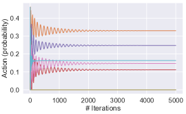
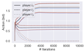
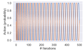
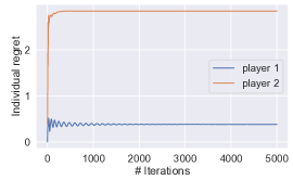
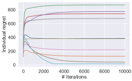
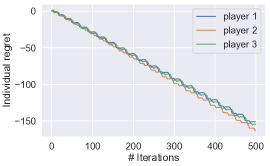
Figure 2: - [Illustrative experiments]: The realized actions (top, each line representing a coordinate of ${x^{i}_{t}}$) and the individual regret (bottom) of a subset of players in a finite two-player zero-sum game (left), a resource allocation auction (middle), and a three-player matching-pennies game [22] (right). All the players use either adaptive OptDA or adaptive DS-OptMD as their learning strategies. We observe convergence of the realized actions and the regrets in the first two examples.

7 Illustrative experiments

In this section we experimentally illustrate our theoretical results through Examples 1 and 2. Precisely, we investigate the following three different setups.

• A finite zero-sum two-player game with $10\times 10$ cost matrix whose elements are drawn uniformly at random from $[-1,+1]$: We let the two players play DS-OptMD respectively with negative entropy and Euclidean regularizers.

• A resource allocation auction (Example 2) with $6$ resources and $20$ bidders: We fix $c_{k}=1$, draw $q_{k}$ and ${\textsl{g}^{i}}$ uniformly at random from $[4,6]$, and draw ${b^{i}}$ uniformly at random from $[5,10]$. Each player runs either OptDA or DS-OptMD and ${h^{i}}(x)=\lVert x\rVert_{2}^{2}/2$ for all $i\in\mathcal{N}$.

• A three-player-matching-pennies game introduced in [22]: Each player has two pure strategies. Player $1$ wants to match the pure strategy of player $2$; player $2$ wants to match the pure strategy of player $3$; and player $3$ wants to match the opposite of the pure strategy of player $1$. Each player receives a loss of $-1$ if they match as desired, and $1$ otherwise. It is straightforward to see that the unique equilibrium is achieved when all the players uniformly randomize. In this game, we let the three players run DS-OptMD with Euclidean regularizer.

As for the learning rates, we fix ${\tau^{i}}=1$ and use the Euclidean norm $\lVert\cdot\rVert_{(i)}=\lVert\cdot\rVert_{2}$ throughout. The results are plotted in Fig. 2. The first two games that we consider are variationally stable, and as predicted by our analysis, we observe the convergence of the iterates and the boundedness of the individual regrets. For the three-player-matching-pennies game, all the players oscillate between the two pure strategies, and have their individual regrets tend to minus infinity. This is consistent with our dichotomy result Theorem 9.

8 Concluding remarks

In this work, we have presented a family of adaptive algorithms for online learning in continuous games that solely utilizes local information received by each player. We showed that these algorithms achieve optimal regret bounds under various conditions, and more importantly, lead to Nash equilibrium when employed by all the players in a variationally stable game.

Many interesting questions remain to be answered. For example, it is known that optimistic algorithms can achieve individual regret much smaller than $\operatorname{\mathcal{O}}(\sqrt{T})$ in general-sum finite games when used by all players [45, 8]. Is this feature shared by our algorithm? Theorem 9 and preliminary experiments suggest that this could be the case. Nonetheless, even this property does not imply that the algorithm effectively generates a ‘good’ sequence of play. In fact, in some cases, the players may benefit more from staying at a Nash equilibrium rather than following a trajectory that lead to $-\infty$ individual regret, and we believe that understanding the dynamics of the algorithm even in the case of no-convergence is an important and challenging direction for future research.

Appendix A Proof of Lemma 1

In this appendix, we present several basic properties of the Bregman divergence, the mirror map, and the Fenchel coupling, before proceeding to prove Lemma 1. For ease of notation, the player index will be dropped in the notation. In particular, we will write $\mathcal{X}$ and $h$ respectively for the player’s action space and the associated regularizer, and we assume that $h$ is $1$-stronlgy convex relative to an ambient norm $\lVert\cdot\rVert$.

A.1 Bregman divergence, mirror map, and Fenchel coupling

We first recall the definition of the Bregman divergence and the Fenchel coupling,

$$D(p,x) =h(p)-h(x)-\langle\operatorname{\nabla}h(x),p-x\rangle,$$

$$F(p,y) =h(p)+h^{\ast}(y)-\langle y,p\rangle,$$

where $h^{\ast}\colon y\to\max_{x\in\mathcal{X}}\langle y,x\rangle-h(x)$ is the Fenchel conjugate of $h$. We also recall that the mirror map induced by $h$ is defined as

$$Q(y)=\operatorname*{arg\,min}_{x\in\mathcal{X}}\langle-y,x\rangle+h(x).$$

The auxiliary results that we are going to present below concerning these three quantities are not new (see e.g., [23, 37, 33] and references therein); however, the set of hypotheses used to obtain them varies widely in the literature, so we still provide the proofs for the sake of completeness.

To begin, our first lemma concerns the optimality condition of the mirror map.

Lemma 10.

Let $h$ be a regularizer on $\mathcal{X}$. Then, for all $x\in\operatorname{dom}\partial h$ and all $y\in\mathbb{R}^{d}$, we have

$$x=Q(y)\iff y\in\partial h(x).$$

Moreover, if $x=Q(y)$, it holds for all $p\in\mathcal{X}$ that

$$\langle\operatorname{\nabla}h(x),x-p\rangle\leq\langle y,x-p\rangle.$$

Proof.

For the first claim, we have by the definition of the mirror map $x=Q(y)$ if and only if $0\in\partial h(x)-y$, i.e., $y\in\partial h(x)$. For the second claim, it suffices to show it holds for all $p\in\operatorname{ri}\mathcal{X}$ (by continuity). To do so, we can define

$$\phi(t)=h(x+t(p-x))-[h(x)+\langle y,x+t(p-x)\rangle].$$

Since $h$ is strongly convex and $y\in\partial h(x)$ by the previous claim, it follows that $\phi(t)\geq 0$ with equality if and only if $t=0$. Moreover, as $\operatorname{ri}\mathcal{X}\subset\operatorname{dom}\partial h$, $\nabla h(x+t(p-x))$ is well-defined and $\psi(t)=\langle\nabla h(x+t(p-x))-y,p-x\rangle$ is a continuous selection of subgradients of $\phi$. Given that $\phi$ and $\psi$ are both continuous on $[0,1]$, it follows that $\phi$ is continuously differentiable and $\phi^{\prime}=\psi$ on $[0,1]$. Thus, with $\phi(t)\geq 0=\phi(0)$ for all $t\in[0,1]$, we conclude that $\phi^{\prime}(0)=\langle\nabla h(x)-y,p-x\rangle\geq 0$, from which our claim follows. ∎

We continue with the “three-point identity” [7] which will be used to derive the recurrent relationship between the divergence measures of different steps.

Lemma 11.

Let $h$ be a regularizer on $\mathcal{X}$. Then, for all $p\in\mathcal{X}$ and all $x,x^{\prime}\in\operatorname{dom}\partial h$, we have

$$\langle\operatorname{\nabla}h(x^{\prime})-\operatorname{\nabla}h(x),x-p\rangle=D(p,x^{\prime})-D(p,x)-D(x,x^{\prime}).$$ (5)

Similarly, writing $x=Q(y)$, for all $p\in\mathcal{X}$ and all $y,y^{\prime}\in\mathbb{R}^{d}$, we have

$$\langle y^{\prime}-y,x-p\rangle=F(p,y^{\prime})-F(p,y)-F(x,y^{\prime}).$$ (6)

Proof.

We start with the Bregman version. By definition,

$$D(p,x^{\prime}) =h(p)-h(x^{\prime})-\langle\nabla h(x^{\prime}),p-x^{\prime}\rangle$$

$$D(p,x) =h(p)-h(x)-\langle\nabla h(x),p-x\rangle$$

$$D(x,x^{\prime}) =h(x)-h(x^{\prime})-\langle\nabla h(x^{\prime}),x-x^{\prime}\rangle.$$

The result then follows by adding the two last lines and subtracting the first. On the other hand, in order to show the Fenchel coupling version we write

$$F(p,y^{\prime}) =h(p)+h^{\ast}(y^{\prime})-\langle y^{\prime},p\rangle$$

$$F(p,y) =h(p)+h^{\ast}(y)-\langle y,p\rangle.$$

Then, by subtracting the above we obtain

$$F(p,y^{\prime})-F(p,y) =h(p)+h^{\ast}(y^{\prime})-\langle y^{\prime},p\rangle-h(p)-h^{\ast}(y)+\langle y,p\rangle$$

$$=h^{\ast}(y^{\prime})-h^{\ast}(y)-\langle y^{\prime}-y,p\rangle$$

$$=h^{\ast}(y^{\prime})-\langle y,Q(y)\rangle+h(Q(y))-\langle y^{\prime}-y,p\rangle$$

$$=h^{\ast}(y^{\prime})-\langle y,x\rangle+h(x)-\langle y^{\prime}-y,p\rangle$$

$$=h^{\ast}(y^{\prime})+\langle y^{\prime}-y,x\rangle-\langle y^{\prime},x\rangle+h(x)-\langle y^{\prime}-y,p\rangle$$

$$=F(x,y^{\prime})+\langle y^{\prime}-y,x-p\rangle$$

and our proof is complete. ∎

Since $x=Q(\operatorname{\nabla}h(x))$ and $F(p,\operatorname{\nabla}h(x))=D(p,x)$, the identity (5) is indeed a special case of (6). In the general case, the Fenchel coupling and the Bregman divergence can be related by the following lemma.

Lemma 12.

Let $h$ be a regularizer on $\mathcal{P}$. Then, for all $p\in\mathcal{P}$ and $y\in\mathbb{R}^{d}$, it holds

$$F(p,y)\geq D(p,Q(y))\geq\frac{\lVert p-Q(y)\rVert^{2}}{2}.$$

Proof.

For the first inequality we have,

$$F(p,y) =h(p)+h^{\ast}(y)-\langle y,p\rangle$$

$$=h(p)-h(Q(y))+\langle y,Q(y)\rangle+\langle y,-p\rangle$$

$$=h(p)-h(Q(y))-\langle y,p-Q(y)\rangle$$

Since $y\in\partial h(Q(y))$, by Lemma 10 we get

$$\langle\nabla h(Q(y)),Q(y)-p\rangle\leq\langle y,Q(y)-p\rangle$$

With all the above we then have

$$F(p,y) =h(p)-h(Q(y))-\langle y,p-Q(y)\rangle$$

$$\geq h(p)-h(Q(y))-\langle\nabla h(Q(y)),p-Q(y)\rangle$$

$$=D(p,Q(y))$$

and the result follows. The second inequality follows directly from the fact that the regularizer $h$ is $1$-strongly convex relative to $\lVert\cdot\rVert$. ∎

Remark.

From the above proof we see that $F(p,y)=h(p)-h(Q(y))-\langle y,p-Q(y)\rangle$. Since $y\in\partial h(Q(y))$ by Lemma 10, Fenchel coupling is also closely related to a generalized version of Bregman divergence which is defined for $p\in\mathcal{X}$, $x\in\operatorname{dom}\partial h$, and $g\in\partial h(x)$ by $D(p,x;g)=h(p)-h(x)-\langle g,p-x\rangle$. This definition is formally introduced in [24], but its use in the literature can be traced back to much earlier work such as [26].

Remark.

By using $x=Q(\operatorname{\nabla}h(x))$ and $F(p,\operatorname{\nabla}h(x))=D(p,x)$, we see immediately that Bregman reciprocity is implied by Fenchel reciprocity.

A.2 Optimistic dual averaging

We first prove Lemma 1 for optimistic dual averaging (OptDA). Its update writes

$$X_{t} =\operatorname*{arg\,min}_{x\in\mathcal{X}}\sum_{s=1}^{t-1}\langle g_{s},x\rangle+\lambda_{t}h(x),$$ (OptDA)

$$X_{t+\frac{1}{2}} =\operatorname*{arg\,min}_{x\in\mathcal{X}}\thinspace\langle g_{t-1},x\rangle+\lambda_{t}D(x,X_{t}).$$

Let us define $Y_{t}=(-1/\lambda_{t})\sum_{s=1}^{t-1}g_{s}$ so that $X_{t}=Q(Y_{t})$. For any $p\in\mathcal{X}$, we can apply the three-point identity for Fenchel coupling (6) to the update of $X_{t+1}$ and get

$$\langle g_{t},X_{t+1}-p\rangle =\langle\lambda_{t}Y_{t}-\lambda_{t+1}Y_{t+1},X_{t+1}-p\rangle$$

$$=\lambda_{t}\langle Y_{t}-Y_{t+1},X_{t+1}-p\rangle+(\lambda_{t+1}-\lambda_{t})\langle 0-Y_{t+1},X_{t+1}-p\rangle$$

$$=\lambda_{t}(F(p,Y_{t})-F(p,Y_{t+1})-F(X_{t+1},Y_{t}))$$

$$~{}~{}+(\lambda_{t+1}-\lambda_{t})(F(p,0)-F(p,Y_{t+1})-F(X_{t+1},0)).$$

As $F(p,0)=h(p)-h(Q(0))=h(p)-\min h$, writing $\varphi(p)=h(p)-\min h$, the above gives

$$\langle g_{t},X_{t+1}-p\rangle\leq\lambda_{t}F(p,Y_{t})-\lambda_{t+1}F(p,Y_{t+1})-\lambda_{t}F(X_{t+1},Y_{t})+(\lambda_{t+1}-\lambda_{t})\varphi(p).$$ (7)

As for the update of $X_{t+\frac{1}{2}}$, we note that $X_{t+\frac{1}{2}}=Q(\operatorname{\nabla}h(X_{t})-g_{t-1}/\lambda_{t})$. Therefore, invoking Lemma 10 gives

$$\langle\operatorname{\nabla}h(X_{t+\frac{1}{2}}),X_{t+\frac{1}{2}}-p\rangle\leq\big{\langle}\operatorname{\nabla}h(X_{t})-\frac{g_{t-1}missing}{\lambda_{t}missing},X_{t+\frac{1}{2}}-p\big{\rangle}.$$

For the specific choice $p\leftarrow X_{t+1}$, using the three-point identity for Bregman divergence (5) we obtain

$$\langle g_{t-1},X_{t+\frac{1}{2}}-X_{t+1}\rangle \leq\lambda_{t}\langle\operatorname{\nabla}h(X_{t})-\operatorname{\nabla}h(X_{t+\frac{1}{2}}),X_{t+\frac{1}{2}}-X_{t+1}\rangle$$ (8)

$$=\lambda_{t}(D(X_{t+1},X_{t})-D(X_{t+1},X_{t+\frac{1}{2}})-D(X_{t+\frac{1}{2}},X_{t})).$$

Since $F(X_{t+1},Y_{t})\geq D(X_{t+1},X_{t})$ by Lemma 12, combining (7) and (8) leads to

$$\langle g_{t},X_{t+\frac{1}{2}}-p\rangle =\langle g_{t}-g_{t-1},X_{t+\frac{1}{2}}-X_{t+1}\rangle+\langle g_{t-1},X_{t+\frac{1}{2}}-X_{t+1}\rangle+\langle g_{t},X_{t+1}-p\rangle$$

$$\leq\lambda_{t}F(p,Y_{t})-\lambda_{t+1}F(p,Y_{t+1})+(\lambda_{t+1}-\lambda_{t})\varphi(p)$$

$$~{}~{}+\langle g_{t}-g_{t-1},X_{t+\frac{1}{2}}-X_{t+1}\rangle-\lambda_{t}D(X_{t+1},X_{t+\frac{1}{2}})-\lambda_{t}D(X_{t+\frac{1}{2}},X_{t}).$$

This proves the generated iterates of OptDA satisfy (2) with ${\psi^{i}_{t}}={F^{i}}(\cdot,{Y^{i}_{t}})$ and ${\varphi^{i}}={h^{i}}-\min{h^{i}}$.

A.3 Dual stabilized optimistic mirror descent

We next prove the generated iterates of dual stabilized optimistic mirror descent (DS-OptMD) satisfy (2) with ${\psi^{i}_{t}}={D^{i}}(\cdot,{X^{i}_{t}})$ and ${\varphi^{i}}={D^{i}}(\cdot,{X^{i}_{1}})$. The algorithm is stated recursively as

$$X_{t+\frac{1}{2}} =\operatorname*{arg\,min}_{x\in\mathcal{X}}\thinspace\langle g_{t-1},x\rangle+\lambda_{t}D(x,X_{t}),$$ (DS-OptMD)

$$X_{t+1} =\operatorname*{arg\,min}_{x\in\mathcal{X}}\thinspace\langle g_{t},x\rangle+\lambda_{t}D(x,X_{t})+(\lambda_{t+1}-\lambda_{t})D(x,X_{1}).$$

By definition of the Bregman divergence and the mirror map, the second step is equivalent to

$$X_{t+1}=Q\left(\frac{\lambda_{t}missing}{\lambda_{t+1}missing}\operatorname{\nabla}h(X_{t})+(1-\frac{\lambda_{t}missing}{\lambda_{t+1}missing})\operatorname{\nabla}h(X_{1})-\frac{g_{t}missing}{\lambda_{t+1}missing}\right).$$

This shows that the update of $X_{t+1}$ consists in fact of a mixing step in the dual space with weight $\lambda_{t}/\lambda_{t+1}$ followed by a standard mirror descent step. Applying Lemma 10 gives

$$\langle\operatorname{\nabla}h(X_{t+1}),X_{t+1}-p\rangle\leq\left\langle\frac{\lambda_{t}missing}{\lambda_{t+1}missing}\operatorname{\nabla}h(X_{t})+(1-\frac{\lambda_{t}missing}{\lambda_{t+1}missing})\operatorname{\nabla}h(X_{1})-\frac{g_{t}missing}{\lambda_{t+1}missing},X_{t+1}-p\right\rangle.$$

We rearrange the terms and use the three-point identity (5) to get

$$\langle g_{t},X_{t+1}-p\rangle \leq\lambda_{t}\langle\operatorname{\nabla}h(X_{t})-\operatorname{\nabla}h(X_{t+1}),X_{t+1}-p\rangle$$ (9)

$$~{}~{}+(\lambda_{t+1}-\lambda_{t})\langle\operatorname{\nabla}h(X_{1})-\operatorname{\nabla}h(X_{t+1}),X_{t+1}-p\rangle$$

$$\leq\lambda_{t}(D(p,X_{t})-D(p,X_{t+1})-D(X_{t+1},X_{t}))$$

$$~{}~{}+(\lambda_{t+1}-\lambda_{t})(D(p,X_{1})-D(p,X_{t+1})-D(X_{t+1},X_{1}))$$

Since $X_{t+\frac{1}{2}}$ is computed exactly as in (OptDA), inequality (8) still holds. We conclude by putting together (9) and (8)

$$\langle g_{t},X_{t+\frac{1}{2}}-p\rangle =\langle g_{t}-g_{t-1},X_{t+\frac{1}{2}}-X_{t+1}\rangle+\langle g_{t-1},X_{t+\frac{1}{2}}-X_{t+1}\rangle+\langle g_{t},X_{t+1}-p\rangle$$

$$\leq\lambda_{t}D(p,X_{t})-\lambda_{t+1}D(p,X_{t+1})+(\lambda_{t+1}-\lambda_{t})D(p,X_{1})$$

$$~{}~{}+\langle g_{t}-g_{t-1},X_{t+\frac{1}{2}}-X_{t+1}\rangle-\lambda_{t}D(X_{t+1},X_{t+\frac{1}{2}})-\lambda_{t}D(X_{t+\frac{1}{2}},X_{t}).$$

This prove Lemma 1 for DS-OptMD. ∎

Appendix B Adaptive optimistic algorithms

In the remainder of the appendix, we consider a broad family of algorithms which we refer to as “optimistic and compatible with dynamic learning rate”. Given a regularizer $h$ and a sequence of non-decreasing positive numbers $(\lambda_{t})_{t\in\mathbb{N}}$, an algorithm of this family produces a sequence of iterates $(X_{s})_{s\in\mathbb{N}/2}$ satisfying that

1. For some non-negative continuous functions $(\psi_{t})_{t\in\mathbb{N}}$ and $\varphi$ defined on ${\mathcal{X}^{i}}$ (the player’s action set), we have, for all $p\in{\mathcal{X}^{i}}$,

   $$\lambda_{t+1}\psi_{t+1}(p) \leq\lambda_{t}\psi_{t}(p)-\langle g_{t},X_{t+\frac{1}{2}}-p\rangle+(\lambda_{t+1}-\lambda_{t})\varphi(p)$$ (10)

   $$~{}+\langle g_{t}-g_{t-1},X_{t+\frac{1}{2}}-X_{t+1}\rangle-\lambda_{t}D(X_{t+1},X_{t+\frac{1}{2}})-\lambda_{t}D(X_{t+\frac{1}{2}},X_{t}),$$

   where $D$ is the associated Bregman divergence of $h$.

2. For every $t\in\mathbb{N}$, $X_{t+\frac{1}{2}}$ is generated by

   $$X_{t+\frac{1}{2}}=\operatorname*{arg\,min}_{x\in{\mathcal{X}^{i}}}\thinspace\langle g_{t-1},x\rangle+\lambda_{t}D(x,X_{t}).$$

By replacing $\varphi$ with $\max(\varphi,\psi_{1})$ if needed, we may assume $\psi_{1}\leq\varphi$ without loss of generality. Thanks to Lemma 1, we know that both (DS-OptMD) and (OptDA) are optimistic and compatible with dynamic learning rate. As another example, it can be proved in a similar way that (OptMD) is optimistic and compatible with dynamic learning rate if $\sup_{p,x\in{\mathcal{X}^{i}}}D(p,x)<+\infty$. In this case, $\psi_{t}=D(\cdot,X_{t})$ and $\varphi\equiv\sup_{p,x\in{\mathcal{X}^{i}}}D(p,x)$.

Since the player’s cost function is convex with respect to its own action by Assumption 1, their regret can be bounded by the linearized regret, which, using (10), can be in turn bounded by

$$\sum_{t=1}^{T}\langle g_{t},X_{t+\frac{1}{2}}-p\rangle \leq\lambda_{T+1}\varphi(p)-\lambda_{T+1}\psi_{T+1}(p)+\sum_{t=1}^{T}\langle g_{t}-g_{t-1},X_{t+\frac{1}{2}}-X_{t+1}\rangle$$ (11)

$$~{}-\sum_{t=1}^{T}\lambda_{t}\left(D(X_{t+1},X_{t+\frac{1}{2}})+D(X_{t+\frac{1}{2}},X_{t})\right).$$

To further obtain (2), we need to invoke Young’s inequality and the strong convexity of $h$. More details can be found in the proof of Theorem 3 (Section C.2). For those results that require the reciprocity conditions, this translates into the following requirement on $\psi_{t}(p)$.

Assumption 2^′.

For some norm $\lVert\cdot\rVert$ and its associated distance function $\operatorname{dist}$, the sequence $(\psi_{t})_{t\in\mathbb{N}}$ satisfies

1. For any $t\in\mathbb{N}$, $\psi_{t}(p)\geq(1/2)\lVert X_{t}-p\rVert^{2}$.

2. For any compact set $\mathcal{K}\in{\mathcal{X}^{i}}$ and $\varepsilon>0$, there exists $r>0$ such that if $\operatorname{dist}(X_{t},\mathcal{K})\leq r$ then $\psi_{t}(\mathcal{K})\coloneqq\min_{p\in\mathcal{K}}\psi_{t}(p)\leq\varepsilon$.

For $\psi_{t}=D(\cdot,X_{t})$ and $\psi_{t}=F(\cdot,Y_{t})$, Assumption 2^′(a) is indeed verified (Lemma 12) and Assumption 2^′(b) is implied by the corresponding reciprocity condition (this can be proved by using some standard arguments of the point-set topology).

In the sequel, we will restate all our results in the case where players “adopt an adaptive optimistic learning strategy”. This means that the player runs an optimistic algorithm that is compatible with dynamic learning rate with a regularizer ${h^{i}}$ and the adaptive scheme (Adapt), and plays ${x^{i}_{t}}={X^{i}_{t+\frac{1}{2}}}$. For ease of presentation, we will take ${\tau^{i}}=1$ throughout, and we will assume that ${h^{i}}$ is $1$-strongly convex relative to $\lVert\cdot\rVert_{(i)}$, but the proof can be easily adapted to general ${\tau^{i}}$ and $\lVert\cdot\rVert_{(i)}$. It will also be convenient to define the norm on the joint action space as

$$\lVert({x^{i}})_{i\in\mathcal{N}}\rVert=\sqrt{\sum_{i=1}^{N}\lVert{x^{i}}\rVert^{2}_{(i)}}.$$ (12)

Appendix C Proofs for regret bounds

C.1 Robustness to adversarial opponent

Theorem 2.

Suppose that Assumption 1 holds, and a player $i\in\mathcal{N}$ adopts an adaptive optimistic learning strategy. If ${\mathcal{P}^{i}}\subseteq{\mathcal{X}^{i}}$ is bounded and $G=\sup_{t}\lVert{g^{i}_{t}}\rVert$, the regret incurred by the player is bounded as ${\operatorname{Reg}^{i}_{T}}({\mathcal{P}^{i}})=\operatorname{\mathcal{O}}(G\sqrt{T}+G^{2})$.

Proof.

By Young’s inequality and the strong convexity of ${h^{i}}$,

$$\begin{multlined}\langle{g^{i}_{t}}-{g^{i}_{t-1}},{X^{i}_{t+\frac{1}{2}}}-{X^{i}_{t+1}}\rangle-{\lambda^{i}_{t}}{D^{i}}({X^{i}_{t+1}},{X^{i}_{t+\frac{1}{2}}})\\ \leq\frac{\lVert{g^{i}_{t}}-{g^{i}_{t-1}}\rVert^{2}_{(i),\ast}missing}{2{\lambda^{i}_{t}}missing}+\frac{{\lambda^{i}_{t}}missing}{2}\lVert{X^{i}_{t+\frac{1}{2}}}-{X^{i}_{t+1}}\rVert^{2}_{(i)}-\frac{{\lambda^{i}_{t}}missing}{2}\lVert{X^{i}_{t+\frac{1}{2}}}-{X^{i}_{t+1}}\rVert^{2}_{(i)}=\frac{{\delta^{i}_{t}}missing}{2{\lambda^{i}_{t}}missing}.\end{multlined}\langle{g^{i}_{t}}-{g^{i}_{t-1}},{X^{i}_{t+\frac{1}{2}}}-{X^{i}_{t+1}}\rangle-{\lambda^{i}_{t}}{D^{i}}({X^{i}_{t+1}},{X^{i}_{t+\frac{1}{2}}})\\ \leq\frac{\lVert{g^{i}_{t}}-{g^{i}_{t-1}}\rVert^{2}_{(i),\ast}missing}{2{\lambda^{i}_{t}}missing}+\frac{{\lambda^{i}_{t}}missing}{2}\lVert{X^{i}_{t+\frac{1}{2}}}-{X^{i}_{t+1}}\rVert^{2}_{(i)}-\frac{{\lambda^{i}_{t}}missing}{2}\lVert{X^{i}_{t+\frac{1}{2}}}-{X^{i}_{t+1}}\rVert^{2}_{(i)}=\frac{{\delta^{i}_{t}}missing}{2{\lambda^{i}_{t}}missing}.$$ (13)

From (11) we then obtain

$$\sum_{t=1}^{T}\langle{g^{i}_{t}},{X^{i}_{t+\frac{1}{2}}}-{p^{i}}\rangle \leq{\lambda^{i}_{T+1}}{\varphi^{i}}({p^{i}})+\frac{1}{2}\sum_{t=1}^{T}\frac{{\delta^{i}_{t}}missing}{{\lambda^{i}_{t}}missing}$$ (14)

$$={\lambda^{i}_{T+1}}{\varphi^{i}}({p^{i}})+\frac{1}{2}\sum_{t=1}^{T}\frac{{\delta^{i}_{t}}missing}{{\lambda^{i}_{t+1}}missing}+\frac{1}{2}\sum_{t=1}^{T}\left(\frac{1}{{\lambda^{i}_{t}}missing}-\frac{1}{{\lambda^{i}_{t+1}}missing}\right){\delta^{i}_{t}}$$

$$\leq(1+{\varphi^{i}}({p^{i}}))\sqrt{1+\sum_{t=1}^{T}{\delta^{i}_{t}}}+2\sum_{t=1}^{T}\left(\frac{1}{{\lambda^{i}_{t}}missing}-\frac{1}{{\lambda^{i}_{t+1}}missing}\right)G^{2}$$

$$\leq(1+{\varphi^{i}}({p^{i}}))\sqrt{1+4G^{2}T}+2G^{2}$$

We have used Lemma 19 in the second to last inequality. We conclude by maximizing the above inequality over ${p^{i}}\in{\mathcal{P}^{i}}$. ∎

C.2 Constant bound on social regret

Theorem 3.

Suppose that Assumption 1 holds and all players $i\in\mathcal{N}$ adopt an adaptive optimistic learning strategy. Then, for every bounded comparator set $\mathcal{P}\subseteq\mathcal{X}$, the players’ social regret is bounded as $\operatorname{Reg}_{T}(\mathcal{P})=\operatorname{\mathcal{O}}(1)$.

Proof.

Let $\mathbf{p}=({p^{i}})_{i\in\mathcal{N}}\in\mathcal{P}$. Since $\mathcal{P}$ is bounded and ${\varphi^{i}}$ is continuous, there exists ${M^{i}}>0$ such that it always holds ${\varphi^{i}}({p^{i}})\leq{M^{i}}$. We start by rewriting the regret bound (11) as

$$\sum_{t=1}^{T}\langle{g^{i}_{t}},{X^{i}_{t+\frac{1}{2}}}-{p^{i}}\rangle \leq{\lambda^{i}_{T+1}}{\varphi^{i}}({p^{i}})-{\lambda^{i}_{T+1}}{\psi^{i}_{T+1}}({p^{i}})$$ (15)

$$~{}~{}-{\lambda^{i}_{1}}{D^{i}}({X^{i}_{3/2}},{X^{i}_{1}})-\frac{{\lambda^{i}_{T}}}{2}{D^{i}}({X^{i}_{T+1}},{X^{i}_{T+\frac{1}{2}}})$$

$$~{}~{}-\sum_{t=2}^{T}\left(\frac{{\lambda^{i}_{t-1}}}{2}{D^{i}}({X^{i}_{t}},{X^{i}_{t-\frac{1}{2}}})+{\lambda^{i}_{t}}{D^{i}}({X^{i}_{t+\frac{1}{2}}},{X^{i}_{t}})\right)$$

$$~{}~{}+\sum_{t=1}^{T}\left(\langle{g^{i}_{t}}-{g^{i}_{t-1}},{X^{i}_{t+\frac{1}{2}}}-{X^{i}_{t+1}}\rangle-\frac{{\lambda^{i}_{t}}missing}{2}{D^{i}}({X^{i}_{t+1}},{X^{i}_{t+\frac{1}{2}}})\right)$$

On one hand, the strong convexity of ${h^{i}}$ implies

$$\lVert{X^{i}_{t+\frac{1}{2}}}-{X^{i}_{t-\frac{1}{2}}}\rVert^{2}_{(i)} \leq 2\lVert{X^{i}_{t+\frac{1}{2}}}-{X^{i}_{t}}\rVert^{2}_{(i)}+2\lVert{X^{i}_{t}}-{X^{i}_{t-\frac{1}{2}}}\rVert^{2}_{(i)}$$ (16)

$$\leq 4{D^{i}}({X^{i}_{t+\frac{1}{2}}},{X^{i}_{t}})+4{D^{i}}({X^{i}_{t}},{X^{i}_{t-\frac{1}{2}}}).$$

On the other hand, similar to (13),

$$\langle{g^{i}_{t}}-{g^{i}_{t-1}},{X^{i}_{t+\frac{1}{2}}}-{X^{i}_{t+1}}\rangle-\frac{{\lambda^{i}_{t}}missing}{2}{D^{i}}({X^{i}_{t+1}},{X^{i}_{t+\frac{1}{2}}})\\ \leq\frac{\lVert{g^{i}_{t}}-{g^{i}_{t-1}}\rVert^{2}_{(i),\ast}missing}{{\lambda^{i}_{t}}missing}.$$ (17)

Combining (15), (16), (17), we obtain

$$\sum_{t=1}^{T}\langle{g^{i}_{t}},{X^{i}_{t+\frac{1}{2}}}-{p^{i}}\rangle \leq{\lambda^{i}_{T+1}}{\varphi^{i}}({p^{i}})-{\lambda^{i}_{T+1}}{\psi^{i}_{T+1}}({p^{i}})$$ (18)

$$~{}~{}+\sum_{t=1}^{T}\frac{\lVert{g^{i}_{t}}-{g^{i}_{t-1}}\rVert^{2}_{(i),\ast}missing}{{\lambda^{i}_{t}}missing}-\frac{1}{8}\sum_{t=2}^{T}{\lambda^{i}_{t-1}}\lVert{X^{i}_{t+\frac{1}{2}}}-{X^{i}_{t-\frac{1}{2}}}\rVert^{2}_{(i)}$$

$$\leq{\lambda^{i}_{T+1}}{M^{i}}+\lVert{V^{i}}(\mathbf{x}_{1})\rVert^{2}_{(i),\ast}$$

$$~{}~{}+\sum_{t=2}^{T}\left(\frac{\lVert{V^{i}}(\mathbf{x}_{t})-{V^{i}}(\mathbf{x}_{t-1})\rVert^{2}_{(i),\ast}missing}{{\lambda^{i}_{t}}missing}-\frac{{\lambda^{i}_{t-1}}missing}{8}\lVert{X^{i}_{t+\frac{1}{2}}}-{X^{i}_{t-\frac{1}{2}}}\rVert^{2}_{(i)}\right).$$

In the current setting, the realized joint action is $\mathbf{x}_{t}=\mathbf{X}_{t+\frac{1}{2}}$. With the norm on $\mathcal{X}$ defined in (12), we have $\sum_{i=1}^{N}\lVert{X^{i}_{t+\frac{1}{2}}}-{X^{i}_{t-\frac{1}{2}}}\rVert^{2}=\lVert\mathbf{X}_{t+\frac{1}{2}}-\mathbf{X}_{t-\frac{1}{2}}\rVert^{2}$. Note that ${\lambda^{i}_{t}}\geq 1$ for all $t$ and $i$ by definition. Summing (18) from $i=1$ to $N$ and maximizing over $p\in\mathcal{P}$ then gives

$$\operatorname{Reg}_{T}(\mathcal{P}) \leq\sum_{i=1}^{N}\left({\lambda^{i}_{T+1}}{M^{i}}+\lVert{V^{i}}(\mathbf{x}_{1})\rVert^{2}_{(i),\ast}\right)$$ (19)

$$~{}~{}+\sum_{t=2}^{T}\left(\sum_{i=1}^{N}\frac{\lVert{V^{i}}(\mathbf{X}_{t+\frac{1}{2}})-{V^{i}}(\mathbf{X}_{t-\frac{1}{2}})\rVert^{2}_{(i),\ast}missing}{{\lambda^{i}_{t}}missing}-\frac{1}{8}\lVert\mathbf{X}_{t+\frac{1}{2}}-\mathbf{X}_{t-\frac{1}{2}}\rVert^{2}\right).$$

In the remainder of the proof, we show that the right-hand side of (19) is bounded from above by some constant. Since all the norms are equivalent in a finite dimensional space, from Assumption 1 we know that for every $i\in\mathcal{N}$, there exists ${L^{i}}>0$ such that for all $\mathbf{x},\mathbf{x}^{\prime}\in\mathcal{X}$,

$$\lVert{V^{i}}(\mathbf{x})-{V^{i}}(\mathbf{x}^{\prime})\rVert_{(i),\ast}\leq{L^{i}}\lVert\mathbf{x}-\mathbf{x}^{\prime}\rVert.$$ (20)

Subsequently,

$$\lVert\mathbf{X}_{t+\frac{1}{2}}-\mathbf{X}_{t-\frac{1}{2}}\rVert^{2}\geq\sum_{i=1}^{N}\frac{1}{N{L^{i}}^{2}}\lVert{V^{i}}(\mathbf{X}_{t+\frac{1}{2}})-{V^{i}}(\mathbf{X}_{t-\frac{1}{2}})\rVert^{2}_{(i),\ast}.$$ (21)

It is thus sufficient to show that for each $i\in\mathcal{N}$, there exists ${C^{i}}\in\mathbb{R}_{+}$ such that for all $T\in\mathbb{N}$,

$${\lambda^{i}_{T+1}}{M^{i}}-\frac{1}{16N{L^{i}}^{2}}\sum_{t=2}^{T}\lVert{V^{i}}(\mathbf{X}_{t+\frac{1}{2}})-{V^{i}}(\mathbf{X}_{t-\frac{1}{2}})\rVert^{2}_{(i),\ast}\leq{C^{i}},$$ (22)

$$\sum_{t=2}^{T}\left(\frac{\lVert{V^{i}}(\mathbf{X}_{t+\frac{1}{2}})-{V^{i}}(\mathbf{X}_{t-\frac{1}{2}})\rVert^{2}_{(i),\ast}missing}{{\lambda^{i}_{t}}missing}-\frac{1}{16N{L^{i}}^{2}}\lVert{V^{i}}(\mathbf{X}_{t+\frac{1}{2}})-{V^{i}}(\mathbf{X}_{t-\frac{1}{2}})\rVert^{2}_{(i),\ast}\right)\leq{C^{i}}.$$ (23)

To simplify the notation, we will write ${\gamma^{i}}=1/(16N{L^{i}}^{2})$. We recall that ${\lambda^{i}_{t}}=\sqrt{1+\sum_{s=1}^{t-1}{\delta^{i}_{t}}}$ where ${\delta^{i}_{t}}=\lVert{g^{i}_{t}}-{g^{i}_{t-1}}\rVert^{2}_{(i),\ast}$. Using the inequality $\sqrt{a+b}\leq\sqrt{a}+\sqrt{b}$, we can bound the left-hand side of (22) as following

$${M^{i}}\sqrt{1+\sum_{s=1}^{T}{\delta^{i}_{t}}}-{\gamma^{i}}\sum_{t=2}^{T}{\delta^{i}_{t}}\leq{M^{i}}\sqrt{1+{\delta^{i}_{1}}}+{M^{i}}\sqrt{\sum_{s=2}^{T}{\delta^{i}_{t}}}-{\gamma^{i}}\sum_{t=2}^{T}{\delta^{i}_{t}}={f^{i}}\left(\sqrt{\sum_{t=2}^{T}{\delta^{i}_{t}}}\right).$$ (24)

where ${f^{i}}\colon\nu\in\mathbb{R}\mapsto-{\gamma^{i}}\nu^{2}+{M^{i}}\nu+{M^{i}}\sqrt{1+{\delta^{i}_{1}}}$ is a quadratic function with negative leading coefficient and is hence bounded from above. This proves (22) by setting ${C^{i}}\geq\max_{\nu\in\mathbb{R}_{+}}{f^{i}}(\nu)$.

Note that $({\lambda^{i}_{t}})_{t\in\mathbb{N}}$ is non-decreasing. Therefore, it either converges to some finite limit or tends to plus infinity. We can thus write $\lim_{t\to+\infty}{\lambda^{i}_{t}}={\lambda^{i}}\in\mathbb{R}_{+}\operatorname*{\cup}\{+\infty\}$. To prove (23), we tackle the two cases separately:

Case 1, ${\lambda^{i}}\in\mathbb{R}_{+}$: In other words, $\sum_{t=2}^{+\infty}{\delta^{i}_{t}}$ is finite. Since ${\lambda^{i}_{t}}\geq 1$, by taking ${C^{i}}\geq\sum_{t=2}^{+\infty}{\delta^{i}_{t}}$ inequality (23) is verified.

Case 2, ${\lambda^{i}}=+\infty$: Then $\lim_{t\to+\infty}1/{\lambda^{i}_{t}}=0$. The quantity $t^{\prime}=\min_{t}\{t:1/{\lambda^{i}_{t}}\leq{\gamma^{i}}\}$ is well-defined and the inequality (23) is satisfied as long as ${C^{i}}\geq\sum_{t=2}^{t^{\prime}-1}(1/{\lambda^{i}_{t}}-{\gamma^{i}}){\delta^{i}_{t}}$.

To summarize, we have proved that (22) and (23) must hold for some ${C^{i}}\in\mathbb{R}_{+}$. Therefore, invoking $\eqref{eq:OptDA-regret-refined}$ and $\eqref{eq:lips-sum}$ we have effectively proved $\operatorname{Reg}_{T}(\mathcal{P})=\operatorname{\mathcal{O}}(1)$. ∎

C.3 Individual regret bound in variationally stable games

Lemma 13.

Let Assumption 1 holds and that all players $i\in\mathcal{N}$ adopt an adaptive optimistic learning strategy. Assume additionally that the game is variationally stable. Then, for every $i\in\mathcal{N}$, the sequence $({\lambda^{i}_{t}})_{t\in\mathbb{N}}$ converges to a finite constant ${\lambda^{i}}\in\mathbb{R}_{+}$ (equivalently, $\sum_{t=1}^{+\infty}{\delta^{i}_{t}}<+\infty$).

Proof.

In this proof we borrow the notations from the proof of Theorem 3. First, summing the left-hand side of (18) from $i=1$ to $N$ leads to $\sum_{t=1}^{T}\langle\mathbf{V}(\mathbf{X}_{t+\frac{1}{2}}),\mathbf{X}_{t+\frac{1}{2}}-\mathbf{p}\rangle$. Since the game is variationally stable, we may take $\mathbf{p}\leftarrow\mathbf{x_{\star}}\in\mathcal{X}_{\star}$ a Nash equilibrium of the game, which gurantees that $\langle\mathbf{V}(\mathbf{x}),\mathbf{x}-\mathbf{x_{\star}}\rangle\geq 0$ for all $\mathbf{x}\in\mathcal{X}$. Summing (18) from $i=1$ to $N$ and using the Lipschitz continuity of the functions, similar to (19), we obtain

$$0 \leq\sum_{i=1}^{N}\left({\lambda^{i}_{T+1}}{\varphi^{i}}({x_{\star}^{i}})+\lVert{V^{i}}(\mathbf{x}_{1})\rVert^{2}_{(i),\ast}\right)$$ (25)

$$~{}~{}+\sum_{t=2}^{T}\left(\sum_{i=1}^{N}\frac{\lVert{V^{i}}(\mathbf{X}_{t+\frac{1}{2}})-{V^{i}}(\mathbf{X}_{t-\frac{1}{2}})\rVert^{2}_{(i),\ast}missing}{{\lambda^{i}_{t}}missing}-\frac{1}{8}\lVert\mathbf{X}_{t+\frac{1}{2}}-\mathbf{X}_{t-\frac{1}{2}}\rVert^{2}\right).$$

Combining (22) and (23) with the above inequality, we deduce that for any $i$, there exists ${\widetilde{C}^{i}}\in\mathbb{R}$ such that for all $T\in\mathbb{N}$,

$${\varphi^{i}}({x_{\star}^{i}})\sqrt{1+\sum_{s=1}^{T}{\delta^{i}_{t}}}-{\gamma^{i}}\sum_{t=2}^{T}{\delta^{i}_{t}}\geq{\widetilde{C}^{i}}.$$

Invoking (24) then gives ${f^{i}}\left(\sqrt{\sum_{t=2}^{T}{\delta^{i}_{t}}}\right)\geq{\widetilde{C}^{i}}$. Since ${f^{i}}$ is a quadratic function with negative leading coefficient, $\lim_{\nu\to+\infty}{f^{i}}(\nu)=-\infty$. Accordingly, $\sum_{t=2}^{+\infty}{\delta^{i}_{t}}$ is finite, which in turn implies ${\lambda^{i}}=\lim_{t\to+\infty}{\lambda^{i}_{t}}<+\infty$. ∎

Theorem 5.

Suppose that Assumption 1 holds and all players $i\in\mathcal{N}$ adopt an adaptive optimistic learning strategy. If the game is variationally stable, then, for every bounded comparator set ${\mathcal{P}^{i}}\subseteq{\mathcal{X}^{i}}$, the individual regret of player $i\in\mathcal{N}$ is bounded as ${\operatorname{Reg}^{i}_{T}}({\mathcal{P}^{i}})=\operatorname{\mathcal{O}}(1)$.

Proof.

From the first line of (14) we have

$$\sum_{t=1}^{T}\langle{g^{i}_{t}},{X^{i}_{t+\frac{1}{2}}}-{p^{i}}\rangle\leq{\lambda^{i}_{T+1}}{\varphi^{i}}({p^{i}})+\frac{1}{2}\sum_{t=1}^{T}\frac{{\delta^{i}_{t}}missing}{{\lambda^{i}_{t}}missing}.$$ (26)

As ${\varphi^{i}}$ is continuous and ${\mathcal{P}^{i}}$ is bounded, ${M^{i}}=\max_{{p^{i}}\in{\mathcal{P}^{i}}}{\varphi^{i}}({p^{i}})$ is well-defined. Moreover, $1/{\lambda^{i}_{t}}\leq 1$ for all $t$. Maximizing (26) over ${p^{i}}\in{\mathcal{P}^{i}}$ then gives

$${\operatorname{Reg}^{i}_{T}}({\mathcal{P}^{i}})\leq{\lambda^{i}_{T+1}}{M^{i}}+\frac{1}{2}\sum_{t=1}^{T}{\delta^{i}_{t}}\leq{\lambda^{i}}{M^{i}}+\frac{1}{2}\sum_{t=1}^{+\infty}{\delta^{i}_{t}},$$

where ${\lambda^{i}}=\lim_{t\to+\infty}{\lambda^{i}_{t}}$ and $\sum_{t=1}^{+\infty}{\delta^{i}_{t}}$ are finite according to Lemma 13. We have thus proved ${\operatorname{Reg}^{i}_{T}}({\mathcal{P}^{i}})=\operatorname{\mathcal{O}}(1)$. ∎

Appendix D Proofs for last-iterate convergence

D.1 Convergence to best response

In this part, we focus on the learning of a single player when the realized actions of the other players converge asymptotically. For ease of notation, the player index $i$ will be dropped when there is no confusion.

Lemma 14.

Let player $i$ adopt an adaptive (optimistic) learning strategy. Then, if the sequence of received feedback is bounded, both the sequences itn) $(\lambda_{t+1}-\lambda_{t})_{t\in\mathbb{N}}$and itn) $(\delta_{t}/\lambda_{t})_{t\in\mathbb{N}}$ tend to zero.

Proof.

This trivially holds if $\lim_{t\to+\infty}\lambda_{t}<+\infty$ (which is equivalent to $\sum_{t=1}^{+\infty}\delta_{t}<+\infty$). Otherwise, we have $\lambda_{t}\to+\infty$. Let $G$ be an upper bound on the received feedback. Since $\delta_{t}\leq 4G^{2}$, we deduce the sequence b) converges to $0$. For the sequence a), we simply note that

$$\lambda_{t+1}-\lambda_{t}=\frac{\lambda^{2}_{t+1}-\lambda^{2}_{t}missing}{\lambda_{t+1}+\lambda_{t}missing}=\frac{\delta_{t}missing}{\lambda_{t+1}+\lambda_{t}missing}\leq\frac{2G^{2}}{\lambda_{t}missing}\xrightarrow{\lambda_{t}\to+\infty}0.$$

∎

Theorem 6.

Suppose that Assumption 1 holds, and a player $i\in\mathcal{N}$ adopts an adaptive optimistic learning strategy that verifies Assumption 2^′. Assume additionally that ${\mathcal{X}^{i}}$ is compact. Then, if all other players’ actions converge to a point ${\mathbf{x}_{\infty}^{-i}}\in\prod_{j\neq i}{\mathcal{X}^{j}}$, player $i$’s realized actions converge to the best response to ${\mathbf{x}_{\infty}^{-i}}$.

Proof.

Let ${x_{\star}^{i}}\in{\mathcal{X}_{\star}^{i}}\coloneqq\operatorname{BR}({\mathbf{x}_{\infty}^{-i}})$. From (10) we derive immediately that

$$\lambda_{t+1}\psi_{t+1}({x_{\star}^{i}}) \leq\lambda_{t}\psi_{t}({x_{\star}^{i}})+(\lambda_{t+1}-\lambda_{t})M+\frac{\delta_{t}missing}{\lambda_{t}missing}$$ (27)

$$~{}~{}-\langle{V^{i}}(\mathbf{X}_{t+\frac{1}{2}}),{X^{i}_{t+\frac{1}{2}}}-{x_{\star}^{i}}\rangle-\frac{\lambda_{t}missing}{4}\lVert{X^{i}_{t+1}}-{X^{i}_{t+\frac{1}{2}}}\rVert^{2}_{(i)},$$

where $M=\max_{{x_{\star}^{i}}\in{\mathcal{X}_{\star}^{i}}}\varphi({x_{\star}^{i}})$. The scalar product term is not necessarily non-negative, but with $\widetilde{\mathbf{X}}_{t+\frac{1}{2}}=({X^{i}_{t+\frac{1}{2}}},{\mathbf{x}_{\infty}^{-i}})$, $\mathbf{x_{\star}}=({x_{\star}^{i}},{\mathbf{x}_{\infty}^{-i}})$, and $R$ the diameter of ${\mathcal{X}^{i}}$, we can decompose

$$\langle{V^{i}}(\mathbf{X}_{t+\frac{1}{2}}),{X^{i}_{t+\frac{1}{2}}}-{x_{\star}^{i}}\rangle =\langle{V^{i}}(\mathbf{X}_{t+\frac{1}{2}})-{V^{i}}(\widetilde{\mathbf{X}}_{t+\frac{1}{2}}),{X^{i}_{t+\frac{1}{2}}}-{x_{\star}^{i}}\rangle+\langle{V^{i}}(\widetilde{\mathbf{X}}_{t+\frac{1}{2}}),{X^{i}_{t+\frac{1}{2}}}-{x_{\star}^{i}}\rangle$$ (28)

$$\geq-R\lVert{V^{i}}(\mathbf{X}_{t+\frac{1}{2}})-{V^{i}}(\widetilde{\mathbf{X}}_{t+\frac{1}{2}})\rVert_{(i),\ast}+{\ell^{i}}(\widetilde{\mathbf{X}}_{t+\frac{1}{2}})-{\ell^{i}}(\mathbf{x_{\star}}).$$

In the inequality we have used the convexity of ${\ell^{i}}(\cdot,{\mathbf{x}_{\infty}^{-i}})$. Since ${\mathcal{X}^{i}}$ is compact and ${V^{i}}$ is continuous, the function

$$f:{\mathbf{x}^{-i}}\mapsto\max_{{p^{i}}\in{\mathcal{X}^{i}}}\lVert{V^{i}}({p^{i}},{\mathbf{x}^{-i}})-{V^{i}}({p^{i}},{\mathbf{x}_{\infty}^{-i}})\rVert_{(i),\ast}$$

is continuous by Berge’s maximum theorem. Therefore $f({\mathbf{X}^{-i}_{t+\frac{1}{2}}})$ converges to $0$ when $t$ goes to infinity. Moreover, from (28) we have

$$\langle{V^{i}}(\mathbf{X}_{t+\frac{1}{2}}),{X^{i}_{t+\frac{1}{2}}}-{x_{\star}^{i}}\rangle\geq-Rf({\mathbf{X}^{-i}_{t+\frac{1}{2}}})+{\ell^{i}}(\widetilde{\mathbf{X}}_{t+\frac{1}{2}})-{\ell^{i}}(\mathbf{x_{\star}}).$$ (29)

Let us write ${\ell_{\star}^{i}}=\min_{{x^{i}}\in{\mathcal{X}^{i}}}{\ell^{i}}({x^{i}},{\mathbf{x}_{\infty}^{-i}})$. Combining (27), (29) and minimizing with respect to ${x_{\star}^{i}}\in{\mathcal{X}_{\star}^{i}}$ leads to

$$\lambda_{t+1}\psi_{t+1}({\mathcal{X}_{\star}^{i}}) \leq\lambda_{t}\psi_{t}({\mathcal{X}_{\star}^{i}})+(\lambda_{t+1}-\lambda_{t})M+\frac{\delta_{t}missing}{\lambda_{t}missing}+Rf({\mathbf{X}^{-i}_{t+\frac{1}{2}}})$$ (30)

$$~{}~{}-({\ell^{i}}(\widetilde{\mathbf{X}}_{t+\frac{1}{2}})-{\ell_{\star}^{i}})-\frac{\lambda_{t}missing}{4}\lVert{X^{i}_{t+1}}-{X^{i}_{t+\frac{1}{2}}}\rVert^{2}_{(i)}.$$

We define $\zeta_{t}=(\lambda_{t+1}-\lambda_{t})M+\delta_{t}/\lambda_{t}+Rf({\mathbf{X}^{-i}_{t+\frac{1}{2}}})$. As ${V^{i}}$ is continuous, ${\mathcal{X}^{i}}$ is compact, and the iterates $({\mathbf{x}^{-i}_{t}})_{t\in\mathbb{N}}$ converges and is hence bounded, the sequence of feedback received by player $i$ is also bounded. Applying Lemma 14 then gives $\lim_{t\to+\infty}\zeta_{t}=0$.

Let us next prove that for any $\varepsilon>0$, we have $\psi_{t}({\mathcal{X}_{\star}^{i}})\leq\varepsilon$ for all $t$ large enough. Since ${\mathcal{X}_{\star}^{i}}\subset{\mathcal{X}^{i}}$ is a compact set, Assumption 2^′(b) ensures the existence of $r>0$ such that if $\operatorname{dist}({X^{i}_{t}},{\mathcal{X}_{\star}^{i}})\leq r$ then $\psi_{t}({\mathcal{X}_{\star}^{i}})\leq\varepsilon$. We distinguish between three different situations:

Case 1, $\operatorname{dist}({X^{i}_{t+\frac{1}{2}}},{\mathcal{X}_{\star}^{i}})\geq r/2$: By convexity of ${\ell^{i}}(\cdot,{\mathbf{x}_{\infty}^{-i}})$ this clearly implies the existence $c>0$ such that ${\ell^{i}}(\widetilde{\mathbf{X}}_{t+\frac{1}{2}})-{\ell_{\star}^{i}}\geq c$ whenever we are in this situation. As $\lim_{t\to+\infty}\zeta_{t}=0$, there exists $t_{1}\in\mathbb{N}$ such that for all $t\geq t_{1}$, $\zeta_{t}\leq c/2$. For any $t\geq t_{1}$, the inequality (30) then gives

$$\lambda_{t+1}\psi_{t+1}({\mathcal{X}_{\star}^{i}})\leq\lambda_{t}\psi_{t}({\mathcal{X}_{\star}^{i}})+\zeta_{t}-c-\frac{\lambda_{t}missing}{4}\lVert{X^{i}_{t+1}}-{X^{i}_{t+\frac{1}{2}}}\rVert^{2}_{(i)}\leq\lambda_{t}\psi_{t}({\mathcal{X}_{\star}^{i}})-\frac{c}{2}.$$

Case 2, $\operatorname{dist}({X^{i}_{t+\frac{1}{2}}},{\mathcal{X}_{\star}^{i}})\leq r/2$ and $\lVert{X^{i}_{t+1}}-{X^{i}_{t+\frac{1}{2}}}\rVert_{(i)}\geq r/2$: We define $t_{2}\in\mathbb{N}$ such that for all $t\geq t_{2}$, $\zeta_{t}\leq r^{2}/32$. Then for $t\geq t_{2}$,

$$\lambda_{t+1}\psi_{t+1}({\mathcal{X}_{\star}^{i}})\leq\lambda_{t}\psi_{t}({\mathcal{X}_{\star}^{i}})+\zeta_{t}-({\ell^{i}}(\widetilde{\mathbf{X}}_{t+\frac{1}{2}})-{\ell_{\star}^{i}})-\frac{r^{2}}{16}\leq\lambda_{t}\psi_{t}({\mathcal{X}_{\star}^{i}})-\frac{r^{2}}{32}.$$

Case 3, $\operatorname{dist}({X^{i}_{t+\frac{1}{2}}},{\mathcal{X}_{\star}^{i}})\leq r/2$ and $\lVert{X^{i}_{t+1}}-{X^{i}_{t+\frac{1}{2}}}\rVert_{(i)}\leq r/2$: By the triangular inequality this implies $\operatorname{dist}({X^{i}_{t+1}},{\mathcal{X}_{\star}^{i}})\leq r$ and thus $\psi_{t+1}({\mathcal{X}_{\star}^{i}})\leq\varepsilon$ by the choice of $r$.

Conclude. Let us consider the sequence $(\rho_{t})_{t\in\mathbb{N}}\in(\mathbb{R}_{+})^{\mathbb{N}}$ defined by $\rho_{t}=\lambda_{t}\psi_{t}({\mathcal{X}_{\star}^{i}})$. For $t\geq\max(t_{1},t_{2})$, whenever we are in Case 1 or 2, we have $\rho_{t+1}\leq\rho_{t}-\min(c/2,r^{2}/32)$. Since $(\rho_{t})_{t\in\mathbb{N}}$ is non-negative, this can not happen for all $t\geq\max(t_{1},t_{2})$; this means Case 3 must happen for some $t^{\prime}\geq\max(t_{1},t_{2})$. Note that for both Case 1 and 2 we get $\psi_{t+1}({\mathcal{X}_{\star}^{i}})\leq\psi_{t}({\mathcal{X}_{\star}^{i}})$. Therefore, with the three cases presented above we see that for all $t\geq t^{\prime}+1$ we have $\psi_{t}({\mathcal{X}_{\star}^{i}})\leq\varepsilon$. We have proved that for any $\varepsilon>0$, the distance measure $\psi_{t}({\mathcal{X}_{\star}^{i}})$ becomes eventually smaller than $\varepsilon$. This means $\lim_{t\to+\infty}\psi_{t}({\mathcal{X}_{\star}^{i}})=0$ and accordingly $\lim_{t\to+\infty}\operatorname{dist}({X^{i}_{t}},{\mathcal{X}_{\star}^{i}})=0$ thanks to Assumption 2^′(a).

We next prove $\lVert{X^{i}_{t+\frac{1}{2}}}-{X^{i}_{t}}\rVert_{(i)}\to 0$. In (10) we may keep the $D({X^{i}_{t+\frac{1}{2}}},{X^{i}_{t}})$ term, then similar to how (30) is derived, we get

$$\lambda_{t}D({X^{i}_{t+\frac{1}{2}}},{X^{i}_{t}})\leq\lambda_{t}\psi_{t}({\mathcal{X}_{\star}^{i}})-\lambda_{t+1}\psi_{t+1}({\mathcal{X}_{\star}^{i}})+\zeta_{t}.$$

This implies

$$\lVert{X^{i}_{t+\frac{1}{2}}}-{X^{i}_{t}}\rVert^{2}_{(i)}\leq 2\left(\psi_{t}({\mathcal{X}_{\star}^{i}})-\psi_{t+1}({\mathcal{X}_{\star}^{i}})+\frac{\zeta_{t}missing}{\lambda_{t}missing}\right).$$

As the right-hand side of the above inequality tends to zero when $t$ goes to infinity, we conclude that $\lVert{X^{i}_{t+\frac{1}{2}}}-{X^{i}_{t}}\rVert_{(i)}\to 0$. As a consequence, $\lim_{t\to+\infty}\operatorname{dist}({X^{i}_{t+\frac{1}{2}}},{\mathcal{X}_{\star}^{i}})=0$. ∎

D.2 Convergence to Nash equilibrium

In this part, we show the convergence of the realized actions to a Nash equilibrium when all the players adopt an adaptive optimistic learning strategy in a variationally stable game. According to Lemma 13, the limit ${\lambda^{i}}=\lim_{t\to+\infty}{\lambda^{i}_{t}}$ is finite in this case.

Lemma 15.

Let Assumption 1 holds and that all players $i\in\mathcal{N}$ adopt an adaptive optimistic learning strategy in a variationally stable game. Then, $\lVert\mathbf{X}_{t+\frac{1}{2}}-\mathbf{X}_{t}\rVert\to 0$ and $\lVert\mathbf{X}_{t}-\mathbf{X}_{t-\frac{1}{2}}\rVert\to 0$ as $t\to+\infty$.

Proof.

Let $\mathbf{x_{\star}}$ be a Nash equilibrium. We apply the regret bound (11) to ${p^{i}}\leftarrow{x_{\star}^{i}}$, and sum these bounds for $i=1$ to $N$, with Young’s inequality (17), we get

$$\frac{1}{2}\sum_{t=1}^{T}\sum_{i=1}^{N}{\lambda^{i}_{t}}\left({D^{i}}({X^{i}_{t+1}},{X^{i}_{t+\frac{1}{2}}})+{D^{i}}({X^{i}_{t+\frac{1}{2}}},{X^{i}_{t}})\right)\leq\sum_{i=1}^{N}\left({\lambda^{i}}{h^{i}}({x_{\star}^{i}})+\sum_{t=1}^{+\infty}\frac{{\delta^{i}_{t}}missing}{{\lambda^{i}_{t}}missing}\right).$$ (31)

The right-hand side of (31) is finite by Lemma 13. With strong convexity of ${h^{i}}$, this implies

$$\sum_{t=1}^{+\infty}\left(\lVert\mathbf{X}_{t+1}-\mathbf{X}_{t+\frac{1}{2}}\rVert^{2}+\lVert\mathbf{X}_{t+\frac{1}{2}}-\mathbf{X}_{t}\rVert^{2}\right)<+\infty.$$

As a consequence, both $\lVert\mathbf{X}_{t+\frac{1}{2}}-\mathbf{X}_{t}\rVert$ and $\lVert\mathbf{X}_{t}-\mathbf{X}_{t-\frac{1}{2}}\rVert$ converge to zero when $t\to+\infty$. ∎

Lemma 16.

Let Assumption 1 holds and that all players $i\in\mathcal{N}$ adopt an adaptive optimistic learning strategy in a variationally stable game. Then, $\sum_{i=1}^{N}{\lambda^{i}}{\psi^{i}_{t}}({x_{\star}^{i}})$ converges for all Nash equilibrium $\mathbf{x_{\star}}\in\mathcal{X}_{\star}$.

Proof.

Let $\mathbf{x_{\star}}$ be a Nash equilibrium. From the descent inequality (10), it is straightforward to show that

$$\sum_{i=1}^{N}{\lambda^{i}_{t+1}}{\psi^{i}_{t+1}}({x_{\star}^{i}}) \leq\sum_{i=1}^{N}{\lambda^{i}_{t}}{\psi^{i}_{t}}({x_{\star}^{i}})-\langle\mathbf{V}(\mathbf{X}_{t+\frac{1}{2}}),\mathbf{X}_{t+\frac{1}{2}}-\mathbf{x_{\star}}\rangle$$

$$~{}~{}+\sum_{i=1}^{N}\left(({\lambda^{i}_{t+1}}-{\lambda^{t}_{t}}){\varphi^{i}}({x_{\star}^{i}})+\frac{{\delta^{i}_{t}}missing}{2{\lambda^{i}_{t}}missing}\right).$$

By the choice of $\mathbf{x_{\star}}$, $\langle\mathbf{V}(\mathbf{X}_{t+\frac{1}{2}}),\mathbf{X}_{t+\frac{1}{2}}-\mathbf{x_{\star}}\rangle\geq 0$. On the other hand, thanks to Lemma 13 we know that the term on the second line is summable. Therefore, by applying Lemma 20, we deduce the convergence of $\sum_{i=1}^{N}{\lambda^{i}_{t}}{\psi^{i}_{t}}({x_{\star}^{i}})$. This in particular implies that ${\psi^{i}_{t}}({x_{\star}^{i}})$ is bounded above for all $i$ and $t$; hence $\sum_{i=1}^{N}({\lambda^{i}}-{\lambda^{i}_{t}}){\psi^{i}_{t}}({x_{\star}^{i}})$ converges to zero, and the convergence of $\sum_{i=1}^{N}{\lambda^{i}}{\psi^{i}_{t}}({x_{\star}^{i}})$ follows immediately. ∎

Theorem 7.

Suppose that Assumption 1 holds and all players $i\in\mathcal{N}$ adopt an adaptive optimistic learning strategy which verifies Assumption 2^′. Then the induced trajectory of play converges to a Nash equilibrium provided that either of the following conditions is satisfied

1. The game is strictly variationally stable.

2. The game is variationally stable and ${h^{i}}$ is subdifferentiable on all of ${\mathcal{X}^{i}}$.

Proof.

We first show that in both cases, a cluster point of $(\mathbf{X}_{t})_{t\in\mathbb{N}}$ is necessarily a Nash equilibrium.

a) Let $\mathbf{x}_{\infty}$ be a cluster point of $(\mathbf{X}_{t})_{t\in\mathbb{N}}$ and $\mathbf{x_{\star}}$ be a Nash equilibrium. The point $\mathbf{x}_{\infty}$ is also a cluster point of $(\mathbf{X}_{t+\frac{1}{2}})_{t\in\mathbb{N}}$ since $\lim_{t\to+\infty}\lVert\mathbf{X}_{t+\frac{1}{2}}-\mathbf{X}_{t}\rVert=0$. From the proof of Theorem 3, we have $\sum_{t=1}^{T}\langle\mathbf{V}(\mathbf{X}_{t+\frac{1}{2}}),\mathbf{X}_{t+\frac{1}{2}}-\mathbf{x_{\star}}\rangle=\operatorname{\mathcal{O}}(1)$. As $\langle\mathbf{V}(\mathbf{X}_{t+\frac{1}{2}}),\mathbf{X}_{t+\frac{1}{2}}-\mathbf{x_{\star}}\rangle\geq 0$ for all $t$, this implies $\lim_{t\to+\infty}\langle\mathbf{V}(\mathbf{X}_{t+\frac{1}{2}}),\mathbf{X}_{t+\frac{1}{2}}-\mathbf{x_{\star}}\rangle=0$. Subsequently, $\langle\mathbf{V}(\mathbf{x}_{\infty}),\mathbf{x}_{\infty}-\mathbf{x_{\star}}\rangle=0$ by the continuity of $\mathbf{V}$, which shows that $\mathbf{x}_{\infty}$ must be a Nash equilibrium by the strict variational stability of the game.

b) Let $\mathbf{x}_{\infty}\in\mathcal{X}$ be a cluster point of $(\mathbf{X}_{t})_{t\in\mathbb{N}}$. We recall that ${X^{i}_{t+\frac{1}{2}}}$ is obtained by

$${X^{i}_{t+\frac{1}{2}}}=\operatorname*{arg\,min}_{x\in{\mathcal{X}^{i}}}\left\{\langle{V^{i}}(\mathbf{X}_{t-\frac{1}{2}}),x\rangle+{\lambda^{i}_{t}}{D^{i}}(x,{X^{i}_{t}})\right\}.$$

For any ${p^{i}}\in{\mathcal{X}^{i}}$, the optimality condition Lemma 10 then gives

$$\langle{V^{i}}(\mathbf{X}_{t-\frac{1}{2}})+{\lambda^{i}_{t}}\operatorname{\nabla}{h^{i}}({X^{i}_{t+\frac{1}{2}}})-{\lambda^{i}_{t}}\operatorname{\nabla}{h^{i}}({X^{i}_{t}}),{p^{i}}-{X^{i}_{t+\frac{1}{2}}}\rangle\geq 0.$$ (32)

Let $(\mathbf{X}_{\omega(t)})_{t\in\mathbb{N}}$ be a subsequence that converges to $\mathbf{x}_{\infty}$. With $\lim_{t\to+\infty}\lVert\mathbf{X}_{t+\frac{1}{2}}-\mathbf{X}_{t}\rVert=0$ and $\lim_{t\to+\infty}\lVert\mathbf{X}_{t}-\mathbf{X}_{t-\frac{1}{2}}\rVert=0$ (Lemma 15), we deduce $\mathbf{X}_{\omega(t)+\frac{1}{2}}\to\mathbf{x}_{\infty}$ and $\mathbf{X}_{\omega(t)-\frac{1}{2}}\to\mathbf{x}_{\infty}$. Since both $\operatorname{\nabla}{h^{i}}$ and ${V^{i}}$ are continuous ($\operatorname{\nabla}{h^{i}}$ is a continuous selection of the subgradients of ${h^{i}}$) and ${\mathcal{X}^{i}}\subset\operatorname{dom}\partial{h^{i}}$, by substituting $t\leftarrow\omega(t)$ in (32) and letting $t$ go to infinity, we get

$$\langle{V^{i}}(\mathbf{x}_{\infty})+{\lambda^{i}}\operatorname{\nabla}{h^{i}}({x_{\infty}^{i}})-{\lambda^{i}}\operatorname{\nabla}{h^{i}}({x_{\infty}^{i}}),{p^{i}}-{x_{\infty}^{i}}\rangle\geq 0.$$

In other words, for all ${p^{i}}\in{\mathcal{X}^{i}}$, it holds that

$$\langle\operatorname{\nabla}_{{x^{i}}}{\ell^{i}}(\mathbf{x}_{\infty}),{p^{i}}-{x_{\infty}^{i}}\rangle\geq 0.$$

Since ${\ell^{i}}$ is convex in ${x^{i}}$ by Assumption 1, the above implies

$${\ell^{i}}({p^{i}},{\mathbf{x}_{\infty}^{-i}})\geq{\ell^{i}}(\mathbf{x}_{\infty}).$$

This is true for all $i\in\mathcal{N}$ and all ${p^{i}}\in{\mathcal{X}^{i}}$, which shows that $\mathbf{x}_{\infty}$ is indeed a Nash equilibrium.

Conclude. Lemma 16 along with Assumption 2^′(a) implies the boundedness of $(\mathbf{X}_{t})_{t\in\mathbb{N}}$. With the above we can readily show that $\operatorname{dist}(\mathbf{x}_{t},\mathcal{X}_{\star})\to 0$ and $\limsup_{t\to+\infty}{\operatorname{\Delta}_{{\mathcal{P}^{i}}}^{i}}(\mathbf{x}_{t})\leq 0$ for all $i$ and every compact set ${\mathcal{P}^{i}}\subset{\mathcal{X}^{i}}$ ($\mathbf{x}_{t}=\mathbf{X}_{t+\frac{1}{2}}$ is the realized action at time $t$).

Below, we further prove the convergence of the iterates to a point using Assumption 2^′(b) and Lemma 16. The sequence $(\mathbf{X}_{t})_{t\in\mathbb{N}}$, being bounded, necessarily possesses a cluster point which we denote by $\mathbf{x}_{\infty}$. We have proved that $\mathbf{x}_{\infty}$ must be a Nash equilibrium. Therefore, by Lemma 16 the sequence $\sum_{i=1}^{N}{\lambda^{i}}{\psi^{i}_{t}}({x_{\infty}^{i}})$ converges. In Assumption 2^′(b), we take $\mathcal{K}\leftarrow\{{x_{\infty}^{i}}\}$ and this means that when ${X^{i}_{t}}$ is close enough to ${x_{\infty}^{i}}$, ${\psi^{i}_{t}}({x_{\infty}^{i}})$ becomes arbitrarily small. Consequently, $\sum_{i=1}^{N}{\lambda^{i}}{\psi^{i}_{t}}({x_{\infty}^{i}})$ can only converge to zero. By invoking Assumption 2^′(a), we then get $\lim_{t\to+\infty}\mathbf{X}_{t}=\mathbf{x}_{\infty}$, or equivalently $\lim_{t\to+\infty}\mathbf{X}_{t+\frac{1}{2}}=\mathbf{x}_{\infty}$. ∎

D.2.1 Finite two-player zero-sum games with adaptive OMWU

We now investigate the specific case of learning in a finite two-player zero-sum game with adaptive (OMWU). We consider the saddle-point formulation of the problem. Let us denote respectively by $\theta\in\operatorname{\Delta}_{m}$ and $\phi\in\operatorname{\Delta}_{n}$ the mixed strategy of the first and the second player. A point $(\theta_{\star},\phi_{\star})$ is a Nash equilibrium if for all $\theta\in\operatorname{\Delta}_{m}$ and $\phi\in\operatorname{\Delta}_{n}$,

$$\theta_{\star}^{\top}A\phi_{\star}\leq\theta^{\top}A\phi_{\star},~{}~{}~{}~{}\theta_{\star}^{\top}A\phi\leq\theta_{\star}^{\top}A\phi_{\star}.$$ (33)

where $A$ is the payoff matrix and without loss of generality we assume $\lVert A\rVert_{\infty}\leq 1$. We define $v=\min_{\theta\in\operatorname{\Delta}_{m}}\max_{\phi\in\operatorname{\Delta}_{n}}\theta^{\top}A\phi$ as the value of the game and we will write ${x}_{[k]}$ for the $k$-th coordinate of $x$. A pure strategy ${\alpha^{i}}$ of player $i$ is called essential if there exists a Nash equilibrium in which player $i$ plays ${\alpha^{i}}$ with positive probability. We have the following lemma from [34].

Lemma 17.

Let $A\in\mathbb{R}^{m\times n}$ be the game matrix for a finite two-player zero-sum game with value $v$. There is a Nash equilibrium $(\theta_{\star},\phi_{\star})$ such that each player plays each of their essential strategies with positive probability, and

$$\forall k\notin\operatorname{supp}(\theta_{\star}),~{}{(A\phi_{\star})}_{[k]}>v,~{}~{}~{}~{}\forall l\notin\operatorname{supp}(\phi_{\star}),~{}{(A^{\top}\theta_{\star})}_{[l]}<v.$$

In the following, we will denote by $x_{\star}=(\theta_{\star},\phi_{\star})$ such an equilibrium. As an immediate consequence, for all $k\in\operatorname{supp}(\theta_{\star})$, ${(A\phi_{\star})}_{[k]}=v$ and for all $l\in\operatorname{supp}(\phi_{\star})$, ${(A^{\top}\theta_{\star})}_{[l]}=v$. We also define

$$\xi=\min\left\{\min_{k\notin\operatorname{supp}(\theta_{\star})}{(A\phi_{\star})}_{[k]}-v,v-\max_{l\notin\operatorname{supp}(\phi_{\star})}{(A^{\top}\theta_{\star})}_{[l]}\right\}>0.$$

Moreover,

$$\xi\leq\frac{\min_{k\notin\operatorname{supp}(\theta_{\star})}{(A\phi_{\star})}_{[k]}-v+v-\max_{l\notin\operatorname{supp}(\phi_{\star})}{(A^{\top}\theta_{\star})}_{[l]}}{2}\leq\frac{\lVert A\phi_{\star}\rVert_{\infty}+\lVert A^{\top}\theta_{\star}\rVert_{\infty}}{2}\leq 1.$$

For any $\widehat{\theta}\in\operatorname{\Delta}_{m}$, we denote by

$$\mathcal{V}_{\widehat{\theta}}=\{\theta\in\operatorname{\Delta}_{m}:\operatorname{supp}(\theta)\subset\operatorname{supp}(\widehat{\theta})\}.$$

the set of the points whose support is included in that of $\widehat{\theta}$. For $\widehat{\phi}\in\operatorname{\Delta}_{n}$, $\mathcal{V}_{\widehat{\phi}}$ is defined in the same way. The next lemma, extracted from [47], is crucial to our proof.

Lemma 18.

Let $\widehat{x}=(\widehat{\theta},\widehat{\phi})\in\operatorname{\Delta}_{m}\times\operatorname{\Delta}_{n}$ satisfy that for all $(\theta,\phi)\in\mathcal{V}_{\theta_{\star}}\times\mathcal{V}_{\phi_{\star}}$,

$$(\theta-\widehat{\theta})^{\top}A\widehat{\phi}+\widehat{\theta}^{\top}A(\widehat{\phi}-\phi)\geq 0.$$ (34)

Then $x^{\prime}=(1-\xi/2)x_{\star}+(\xi/2)\widehat{x}$ is also a Nash equilibrium.

Proof.

We rewrite the left-hand side of (34) as

$$(\theta-\widehat{\theta})^{\top}A\widehat{\phi}+\widehat{\theta}^{\top}A(\widehat{\phi}-\phi)=\theta^{\top}A\widehat{\phi}-v+v-\widehat{\theta}^{\top}A\phi=\theta^{\top}A(\widehat{\phi}-\phi_{\star})+(\theta_{\star}-\widehat{\theta})^{\top}A\phi.$$ (35)

The second inequality holds because $(\theta,\phi)\in\mathcal{V}_{\theta_{\star}}\times\mathcal{V}_{\phi_{\star}}$. With the choice $(\theta,\phi)\leftarrow(\theta_{\star},\phi_{\star})$ and (34) we then get

$$\theta_{\star}^{\top}A(\widehat{\phi}-\phi_{\star})+(\theta_{\star}-\widehat{\theta})^{\top}A\phi_{\star}\geq 0.$$

This implies

$$\theta_{\star}^{\top}A(\widehat{\phi}-\phi_{\star})=(\theta_{\star}-\widehat{\theta})^{\top}A\phi_{\star}=0$$ (36)

by the definition of Nash equilibrium (33).

We next prove that $(\theta_{\star},\phi^{\prime})$ is also a Nash equilibrium with $\phi^{\prime}=(1-\xi/2)\phi_{\star}+(\xi/2)\widehat{\phi}$. From (36) we already have

$$\theta_{\star}^{\top}A\phi^{\prime}=\theta_{\star}^{\top}A\phi_{\star}=v=\max_{\phi\in\operatorname{\Delta}_{n}}\theta_{\star}^{\top}A\phi.$$

It remains to show that $\theta_{\star}^{\top}A\phi^{\prime}=\min_{\theta\in\operatorname{\Delta}_{m}}\theta^{\top}A\phi^{\prime}$. By choosing $\phi=\phi_{\star}$ in (35), we know that for all $\theta\in\mathcal{V}_{\theta_{\star}}$, it holds $\theta^{\top}A(\widehat{\phi}-\phi_{\star})\geq 0$. In other words,

$$\forall k\in\operatorname{supp}(\theta_{\star}),~{}~{}{(A(\widehat{\phi}-\phi_{\star}))}_{[k]}\geq 0$$ (37)

Let $\theta\in\operatorname{\Delta}_{m}$. We decompose

$$\theta^{\top}A\phi^{\prime}=\sum_{k\in\operatorname{supp}(\theta_{\star})}{\theta}_{[k]}{(A\phi^{\prime})}_{[k]}+\sum_{k\notin\operatorname{supp}(\theta_{\star})}{\theta}_{[k]}{(A\phi^{\prime})}_{[k]}.$$ (38)

The first term can be bounded below using (37),

$$\sum_{k\in\operatorname{supp}(\theta_{\star})}{\theta}_{[k]}{(A\phi^{\prime})}_{[k]}=\sum_{k\in\operatorname{supp}(\theta_{\star})}\left(\frac{\xi}{2}\,{\theta}_{[k]}{(A(\widehat{\phi}-\phi_{\star}))}_{[k]}+{\theta}_{[k]}{(A\phi_{\star})}_{[k]}\right)\geq\sum_{k\in\operatorname{supp}(\theta_{\star})}{\theta}_{[k]}v.$$ (39)

We proceed to lower bound the second term

$$\sum_{k\notin\operatorname{supp}(\theta_{\star})}{\theta}_{[k]}{(A\phi^{\prime})}_{[k]} \geq\sum_{k\notin\operatorname{supp}(\theta_{\star})}\left({\theta}_{[k]}{(A\phi_{\star})}_{[k]}-\frac{\xi}{2}\,\lvert{\theta}_{[k]}{(A(\widehat{\phi}-\phi_{\star}))}_{[k]}\rvert\right)$$ (40)

$$\geq\sum_{k\notin\operatorname{supp}(\theta_{\star})}\left({\theta}_{[k]}{(A\phi_{\star})}_{[k]}-\frac{\xi}{2}\,{\theta}_{[k]}\lVert A\rVert_{\infty}\lVert\widehat{\phi}-\phi_{\star}\rVert_{1}\right)$$

$$\geq\sum_{k\notin\operatorname{supp}(\theta_{\star})}{\theta}_{[k]}({(A\phi_{\star})}_{[k]}-\xi)$$

$$\geq\sum_{k\notin\operatorname{supp}(\theta_{\star})}{\theta}_{[k]}v.$$

In the last inequality we use the definition of $\xi$. Combining (38), (39), and (40) we have $\theta^{\top}A\phi^{\prime}\geq v=\theta_{\star}^{\top}A\phi^{\prime}$. We have therefore proved that $(\theta_{\star},\phi^{\prime})$ is a Nash equilibrium. In the same way we can show that with $\theta^{\prime}=(1-\xi/2)\theta_{\star}+(\xi/2)\widehat{\theta}$, the point $(\theta^{\prime},\phi_{\star})$ is also a Nash equilibrium. We then conclude that $x^{\prime}=(\theta^{\prime},\phi^{\prime})$ is indeed a Nash equilibrium. ∎

In the following we analyse the case where both ${h^{1}}$ and ${h^{2}}$ are negative entropy regularizers (i.e., both players play adaptive OMWU). The case where one is negative entropy regularizer and the other satisfies that ${\mathcal{X}^{i}}\subset\operatorname{dom}\partial{h^{i}}$ can be proved similarly. The Bregman divergence for the negative entropy regularizer is the KL divergence which we will denote by $D_{\mathrm{KL}}$. We take $\operatorname{\nabla}{h^{1}}\colon({\theta}_{[k]})_{k\in\{1,\ldots,m\}}\to(-\log{\theta}_{[k]})_{k\in\{1,\ldots,m\}}$ and $\operatorname{\nabla}{h^{2}}\colon({\phi}_{[l]})_{l\in\{1,\ldots,m\}}\to(-\log{\phi}_{[l]})_{l\in\{1,\ldots,n\}}$.

See 8

Proof.

Consider the solution $x_{\star}=(\theta_{\star},\phi_{\star})$ that we have chosen using Lemma 17. By Lemma 16 we know that ${\lambda^{1}}D_{\mathrm{KL}}(\theta_{\star},\theta_{t})+{\lambda^{2}}D_{\mathrm{KL}}(\phi_{\star},\phi_{t})$ are bounded above. This implies that for all $k\in\operatorname{supp}(\theta_{\star})$ and $l\in\operatorname{supp}(\phi_{\star})$, the coordinates $\theta_{t,[k]}$ and $\phi_{t,[l]}$ are bounded below. In particular, for any cluster point $x_{\infty}=(\theta_{\infty},\phi_{\infty})$, we have $\operatorname{supp}(\theta_{\star})\subset\operatorname{supp}(\theta_{\infty})$ and $\operatorname{supp}(\phi_{\star})\subset\operatorname{supp}(\phi_{\infty})$.

We will proceed to prove the sequence of produced iterates only has one cluster point. We first use the optimality condition (32) but only apply it to ${p^{1}}\leftarrow\theta\in\mathcal{V}(\theta_{\star})$. This gives

$$\sum_{k\in\operatorname{supp}(\theta_{\star})}({{V^{1}}(\mathbf{X}_{t-\frac{1}{2}})}_{[k]}+{\lambda^{1}_{t}}(\log(\theta_{t,[k]})-\log(\theta_{t+\frac{1}{2},[k]})))({\theta}_{[k]}-\theta_{t+\frac{1}{2},[k]})\geq 0$$ (41)

We consider a subsequence that goes to a cluster point $x_{\infty}=(\theta_{\infty},\phi_{\infty})$. Since ${\theta_{\infty}}_{[k]}>0$ for all $k\in\operatorname{supp}(\theta_{\star})$ and both $\lVert\mathbf{X}_{t}-\mathbf{X}_{t-\frac{1}{2}}\rVert$ and $\lVert\mathbf{X}_{t+\frac{1}{2}}-\mathbf{X}_{t}\rVert$ go to zero (Lemma 15), (41) implies

$$\sum_{k\in\operatorname{supp}(\theta_{\star})}{{V^{1}}(\mathbf{x}_{\infty})}_{[k]}({\theta}_{[k]}-{\theta_{\infty}}_{[k]})\geq 0.$$

Equivalently, $(\theta-\theta_{\infty})^{\top}A\phi_{\infty}\geq 0$. In the same way, for all $\phi\in\mathcal{V}(\phi_{\star})$ we have $\theta_{\infty}^{\top}A(\phi_{\infty}-\phi)\geq 0$. We can thus apply Lemma 18 and we know that $(\theta_{\star}^{\prime},\phi_{\star}^{\prime})=(1-\xi/2)x_{\star}+(\xi/2)x_{\infty}$ is also a Nash equilibrium. By the choice of $x_{\star}$, we have $\operatorname{supp}(\theta_{\star}^{\prime})\subset\operatorname{supp}(\theta_{\star})$ and $\operatorname{supp}(\phi_{\star}^{\prime})\subset\operatorname{supp}(\phi_{\star})$. Subsequently, $\operatorname{supp}(\theta_{\star})=\operatorname{supp}(\theta_{\infty})$ and $\operatorname{supp}(\phi_{\star})=\operatorname{supp}(\phi_{\infty})$.

Using Lemma 16, we can define

$$\rho =\lim_{t\to+\infty}{\lambda^{1}}D_{\mathrm{KL}}(\theta_{\star},\theta_{t})+{\lambda^{2}}D_{\mathrm{KL}}(\phi_{\star},\phi_{t})$$

$$\rho^{\prime} =\lim_{t\to+\infty}{\lambda^{2}}D_{\mathrm{KL}}(\theta_{\star}^{\prime},\theta_{t})+{\lambda^{2}}D_{\mathrm{KL}}(\phi_{\star}^{\prime},\phi_{t}).$$

Since $\operatorname{supp}(\theta_{\star})=\operatorname{supp}(\theta_{\infty})$ and $\operatorname{supp}(\phi_{\star})=\operatorname{supp}(\phi_{\infty})$, we can use the continuity of the KL divergence with respect to the second variable and deduce that ${\lambda^{1}}D_{\mathrm{KL}}(\theta_{\star},\theta_{\infty})+{\lambda^{2}}D_{\mathrm{KL}}(\phi_{\star},\phi_{\infty})=\rho$. Similarly, ${\lambda^{1}}D_{\mathrm{KL}}(\theta_{\star}^{\prime},\theta_{\infty})+{\lambda^{2}}D_{\mathrm{KL}}(\phi_{\star}^{\prime},\phi_{\infty})=\rho^{\prime}$. These two equations also hold if we consider another cluster point $x_{\infty}^{\prime}=(\theta_{\infty}^{\prime},\phi_{\infty}^{\prime})$. As a consequence,

$$\begin{multlined}{\lambda^{1}}\sum_{k\in\operatorname{supp}(\theta_{\star})}{\theta_{\star}}_{[k]}\log{\theta_{\infty}}_{[k]}+{\lambda^{2}}\sum_{l\in\operatorname{supp}(\phi_{\star})}{\phi_{\star}}_{[l]}\log{\phi_{\infty}}_{[l]}\\ ={\lambda^{1}}\sum_{k\in\operatorname{supp}(\theta_{\star})}{\theta_{\star}}_{[k]}\log{\theta_{\infty}^{\prime}}_{[k]}+{\lambda^{2}}\sum_{l\in\operatorname{supp}(\phi_{\star})}{\phi_{\star}}_{[l]}\log{\phi_{\infty}^{\prime}}_{[l]},\end{multlined}{\lambda^{1}}\sum_{k\in\operatorname{supp}(\theta_{\star})}{\theta_{\star}}_{[k]}\log{\theta_{\infty}}_{[k]}+{\lambda^{2}}\sum_{l\in\operatorname{supp}(\phi_{\star})}{\phi_{\star}}_{[l]}\log{\phi_{\infty}}_{[l]}\\ ={\lambda^{1}}\sum_{k\in\operatorname{supp}(\theta_{\star})}{\theta_{\star}}_{[k]}\log{\theta_{\infty}^{\prime}}_{[k]}+{\lambda^{2}}\sum_{l\in\operatorname{supp}(\phi_{\star})}{\phi_{\star}}_{[l]}\log{\phi_{\infty}^{\prime}}_{[l]},$$ (42)

and

$$\begin{multlined}{\lambda^{1}}\sum_{k\in\operatorname{supp}(\theta_{\star})}{\theta_{\star}^{\prime}}_{[k]}\log{\theta_{\infty}}_{[k]}+{\lambda^{2}}\sum_{l\in\operatorname{supp}(\phi_{\star})}{\phi_{\star}^{\prime}}_{[l]}\log{\phi_{\infty}}_{[l]}\\ ={\lambda^{1}}\sum_{k\in\operatorname{supp}(\theta_{\star})}{\theta_{\star}^{\prime}}_{[k]}\log{\theta_{\infty}^{\prime}}_{[k]}+{\lambda^{2}}\sum_{l\in\operatorname{supp}(\phi_{\star})}{\phi_{\star}^{\prime}}_{[l]}\log{\phi_{\infty}^{\prime}}_{[l]},\end{multlined}{\lambda^{1}}\sum_{k\in\operatorname{supp}(\theta_{\star})}{\theta_{\star}^{\prime}}_{[k]}\log{\theta_{\infty}}_{[k]}+{\lambda^{2}}\sum_{l\in\operatorname{supp}(\phi_{\star})}{\phi_{\star}^{\prime}}_{[l]}\log{\phi_{\infty}}_{[l]}\\ ={\lambda^{1}}\sum_{k\in\operatorname{supp}(\theta_{\star})}{\theta_{\star}^{\prime}}_{[k]}\log{\theta_{\infty}^{\prime}}_{[k]}+{\lambda^{2}}\sum_{l\in\operatorname{supp}(\phi_{\star})}{\phi_{\star}^{\prime}}_{[l]}\log{\phi_{\infty}^{\prime}}_{[l]},$$ (43)

With $(\theta_{\star}^{\prime},\phi_{\star}^{\prime})=(1-\xi/2)x_{\star}+(\xi/2)x_{\infty}$ and $\xi>0$, using (42) and (43) we get

$$\begin{multlined}{\lambda^{1}}\sum_{k\in\operatorname{supp}(\theta_{\star})}{\theta_{\infty}}_{[k]}\log{\theta_{\infty}}_{[k]}+{\lambda^{2}}\sum_{l\in\operatorname{supp}(\phi_{\star})}{\phi_{\infty}}_{[l]}\log{\phi_{\infty}}_{[l]}\\ ={\lambda^{1}}\sum_{k\in\operatorname{supp}(\theta_{\star})}{\theta_{\infty}}_{[k]}\log{\theta_{\infty}^{\prime}}_{[k]}+{\lambda^{2}}\sum_{l\in\operatorname{supp}(\phi_{\star})}{\phi_{\infty}}_{[l]}\log{\phi_{\infty}^{\prime}}_{[l]},\end{multlined}{\lambda^{1}}\sum_{k\in\operatorname{supp}(\theta_{\star})}{\theta_{\infty}}_{[k]}\log{\theta_{\infty}}_{[k]}+{\lambda^{2}}\sum_{l\in\operatorname{supp}(\phi_{\star})}{\phi_{\infty}}_{[l]}\log{\phi_{\infty}}_{[l]}\\ ={\lambda^{1}}\sum_{k\in\operatorname{supp}(\theta_{\star})}{\theta_{\infty}}_{[k]}\log{\theta_{\infty}^{\prime}}_{[k]}+{\lambda^{2}}\sum_{l\in\operatorname{supp}(\phi_{\star})}{\phi_{\infty}}_{[l]}\log{\phi_{\infty}^{\prime}}_{[l]},$$

Note that we also have $\operatorname{supp}(\theta_{\star})=\operatorname{supp}(\theta_{\infty}^{\prime})$ and $\operatorname{supp}(\phi_{\star})=\operatorname{supp}(\phi_{\infty}^{\prime})$. The above is thus equivalent to

$${\lambda^{1}}D_{\mathrm{KL}}(\theta_{\infty},\theta_{\infty}^{\prime})+{\lambda^{2}}D_{\mathrm{KL}}(\phi_{\infty},\phi_{\infty}^{\prime})=0$$

This shows $x_{\infty}=x_{\infty}^{\prime}$, and therefore $(\mathbf{X}_{t})_{t\in\mathbb{N}}$ has only one cluster point; in other words, the algorithm converges (recall that $\lim_{t\to+\infty}\lVert\mathbf{X}_{t+\frac{1}{2}}-\mathbf{X}_{t}\rVert=0$). To conclude, we note that if a no regret learning algorithm converges, it must converge to a Nash equilibrium. In fact, for all $\theta\in\operatorname{\Delta}_{m}$, we have $\sum_{t=1}^{T}\langle{V^{1}}(\mathbf{X}_{t+\frac{1}{2}}),\theta_{t+\frac{1}{2}}-\theta\rangle=\operatorname{\mathnormal{o}}(T)$ and thus $\liminf_{t\to+\infty}\langle{V^{1}}(\mathbf{X}_{t+\frac{1}{2}}),\theta_{t+\frac{1}{2}}-\theta\rangle\leq 0$. However, $\lim_{t\to+\infty}\langle{V^{1}}(\mathbf{X}_{t+\frac{1}{2}}),\theta_{t+\frac{1}{2}}-\theta\rangle=\langle{V^{1}}(x_{\infty}),\theta_{\infty}-\theta\rangle$. This shows $\langle{V^{1}}(x_{\infty}),\theta_{\infty}-\theta\rangle\leq 0$ for all $\theta\in\operatorname{\Delta}_{m}$ and thus $\theta_{\infty}$ is a best response to $\phi_{\infty}$. The same argument also applies to the second player; accordingly, $x_{\infty}$ is indeed a Nash equilibrium. ∎

D.3 A dichotomy result for general convex games

Below we prove a variant of Theorem 9 which does not require the compactness assumption. Theorem 9 is a direct corollary of this variant.

Theorem 9^′.

Suppose that Assumption 1 holds and all players $i\in\mathcal{N}$ adopt an adaptive optimistic learning strategy. Assume additionally that ${\mathcal{X}^{i}}\subset\operatorname{dom}\partial{h^{i}}$. Then one of the following holds:

1. For every $i\in\mathcal{N}$ and every compact set ${\mathcal{P}^{i}}\in{\mathcal{X}^{i}}$, the individual regret ${\operatorname{Reg}^{i}_{T}}({\mathcal{P}^{i}})$ is bounded above i.e., ${\operatorname{Reg}^{i}_{T}}({\mathcal{P}^{i}})=\operatorname{\mathcal{O}}(1)$. Moreover, every cluster point of the realized actions is a Nash equilibrium of the game.

2. For every compact set $\mathcal{P}\subset\mathcal{X}$, the social regret with respect it tends to minus infinity when $t\to+\infty$, i.e., $\lim_{t\to+\infty}\operatorname{Reg}_{T}(\mathcal{P})=-\infty$.

Proof.

By Lipschitz continuity of ${V^{i}}$, there exists ${L^{i}}>0$ such that

$$\lVert{V^{i}}(\mathbf{X}_{t+\frac{1}{2}})-{V^{i}}(\mathbf{X}_{t-\frac{1}{2}})\rVert_{(i),\ast}\leq{L^{i}}\lVert\mathbf{X}_{t+\frac{1}{2}}-\mathbf{X}_{t-\frac{1}{2}}\rVert\leq{L^{i}}(\lVert\mathbf{X}_{t+\frac{1}{2}}-\mathbf{X}_{t}\rVert+\lVert\mathbf{X}_{t}-\mathbf{X}_{t-\frac{1}{2}}\rVert).$$

We set ${\delta^{\prime i}_{t}}=2{L^{i}}^{2}(\lVert\mathbf{X}_{t+\frac{1}{2}}-\mathbf{X}_{t}\rVert^{2}+\lVert\mathbf{X}_{t}-\mathbf{X}_{t-\frac{1}{2}}\rVert^{2})$ for $t\geq 2$ so that ${\delta^{i}_{t}}\leq{\delta^{\prime i}_{t}}$. We also define ${\delta^{\prime i}_{1}}={\delta^{i}_{1}}=\lVert{V^{i}}(\mathbf{x}_{1})\rVert^{2}_{(i),\ast}$, ${\gamma^{i}}=1/(16N{L^{i}}^{2})$, and ${M^{i}}=\max_{{p^{i}}\in{\mathcal{P}^{i}}}{\varphi^{i}}({p^{i}})$. Then, from the regret bound (11), similar to how (19) is derived, we deduce

$$\operatorname{Reg}_{T}(\mathcal{P}) \leq\sum_{i=1}^{N}\left({\lambda^{i}_{T+1}}{M^{i}}+\lVert{V^{i}}(\mathbf{x}_{1})\rVert^{2}_{(i),\ast}\right)$$

$$~{}~{}+\sum_{t=2}^{T}\left(\sum_{i=1}^{N}\frac{{\delta^{i}_{t}}missing}{{\lambda^{i}_{t}}missing}-\frac{1}{4}\left(\lVert\mathbf{X}_{t+\frac{1}{2}}-\mathbf{X}_{t}\rVert^{2}+\lVert\mathbf{X}_{t}-\mathbf{X}_{t-\frac{1}{2}}\rVert^{2}\right)\right)$$

$$\leq\sum_{i=1}^{N}\left({M^{i}}\sqrt{1+\sum_{t=1}^{T}{\delta^{\prime i}_{t}}}+{\delta^{i}_{1}}-{\gamma^{i}}\sum_{t=2}^{T}{\delta^{\prime i}_{t}}\right)+\sum_{t=2}^{T}\sum_{i=1}^{N}\left(\frac{{\delta^{i}_{t}}missing}{{\lambda^{i}_{t}}missing}-{\gamma^{i}}{\delta^{i}_{t}}\right).$$

Following the reasoning of the proof of Theorem 3, we know there exists a constant $C$ such that for all $T\in\mathbb{N}$,

$$\operatorname{Reg}_{T}(\mathcal{P})\leq C+{f^{1}}\left(\sqrt{\sum_{t=2}^{T}{\delta^{\prime 1}_{t}}}\right),$$

where ${f^{1}}\colon\nu\in\mathbb{R}\mapsto-{\gamma^{1}}\nu^{2}+{M^{1}}\nu$ is quadratic and has negative leading coefficient. Therefore, $\operatorname{Reg}_{T}(\mathcal{P})\to-\infty$ when $\sum_{t=1}^{+\infty}{\delta^{\prime 1}_{t}}=+\infty$, and this corresponds to the situation 2.

Otherwise, $\sum_{t=1}^{+\infty}(\lVert\mathbf{X}_{t+\frac{1}{2}}-\mathbf{X}_{t}\rVert^{2}+\lVert\mathbf{X}_{t}-\mathbf{X}_{t-\frac{1}{2}}\rVert^{2})<+\infty$ and this implies

1. $\lim_{t\to+\infty}\lVert\mathbf{X}_{t+\frac{1}{2}}-\mathbf{X}_{t}\rVert^{2}=0$;

2. $\lim_{t\to+\infty}\lVert\mathbf{X}_{t}-\mathbf{X}_{t-\frac{1}{2}}\rVert^{2}=0$;

3. for all $i\in\mathcal{N}$, $\sum_{t=1}^{+\infty}{\delta^{i}_{t}}<+\infty$ and hence ${\lambda^{i}}=\lim_{t\to+\infty}{\lambda^{i}_{t}}<+\infty$.

To conclude, we prove the boundedness of individual regrets as in the proof of Theorem 5 and that every cluster point of $(\mathbf{X}_{t+\frac{1}{2}})_{t\in\mathbb{N}}$ is a Nash equilibrium as in the proof of Theorem 7 (case a). ∎

Appendix E Technical lemmas for numerical sequences

In this appendix we provide two basic lemmas for numerical sequences, one for bounding the adversarial regret of adaptive methods [4, Lemma 3.5], and the other for the analysis of quasi-Fejér sequence [12, Lemma 3.1].

Lemma 19.

For any real numbers $\nu_{1},\ldots,\nu_{T}$ such that $\sum_{s=1}^{t}\nu_{s}>0$ for all $t\in\{1,\ldots,T\}$, it holds

$$\sum_{t=1}^{T}\frac{\nu_{t}}{\sqrt{\sum_{s=1}^{t}\nu_{s}}}\leq 2\sqrt{\sum_{t=1}^{T}\nu_{t}}.$$

Proof.

The function $y\in\mathbb{R}^{+}\mapsto\sqrt{y}$ being concave and has derivative $y\mapsto 1/(2\sqrt{y})$, it holds for every $z\geq 0$,

$$\sqrt{z}\leq\sqrt{y}+\frac{1}{2\sqrt{y}}(z-y).$$

Take $y=\sum_{s=1}^{t}\nu_{s}$ and $z=\sum_{s=1}^{t-1}\nu_{s}$ gives

$$2\sqrt{\sum_{s=1}^{t-1}\nu_{s}}+\frac{\nu_{t}}{\sqrt{\sum_{s=1}^{t}\nu_{s}}}\leq 2\sqrt{\sum_{s=1}^{t}\nu_{s}}.$$

We conclude by summing the inequality from $t=2$ to $t=T$ and using $\sqrt{\nu_{1}}\leq 2\sqrt{\nu_{1}}$. ∎

Lemma 20.

Let $(D_{t})_{t\in\mathbb{N}}\in\mathbb{R}_{+}^{\mathbb{N}}$ be a non-negative sequence and $(\chi_{t})_{t\in\mathbb{N}}\in\mathbb{R}_{+}^{\mathbb{N}}$ be summable such that, for all $t\in\mathbb{N}$,

$$D_{t+1}\leq D_{t}+\chi_{t}.$$ (44)

Then, $(D_{t})_{t\in\mathbb{N}}$ converges.

Proof.

Since $(\chi_{t})_{t\in\mathbb{N}}$ is summable, we can define $D^{\prime}_{t}=D_{t}+\sum_{s=t}^{+\infty}\chi_{s}\in\mathbb{R}_{+}$. Inequality (44) then implies $D^{\prime}_{t+1}\leq D^{\prime}_{t}$. Therefore, $(D^{\prime}_{t})_{t\in\mathbb{N}}$ converges, and accordingly $(D_{t})_{t\in\mathbb{N}}$ converges. ∎

References

- Abernethy et al. [2018] Jacob Abernethy, Kevin A Lai, Kfir Y Levy, and Jun-Kun Wang. Faster rates for convex-concave games. In Conference On Learning Theory, pages 1595–1625. PMLR, 2018.
- Antonakopoulos et al. [2019] Kimon Antonakopoulos, E. Veronica Belmega, and Panayotis Mertikopoulos. An adaptive mirror-prox algorithm for variational inequalities with singular operators. In NeurIPS ’19: Proceedings of the 33rd International Conference on Neural Information Processing Systems, 2019.
- Antonakopoulos et al. [2021] Kimon Antonakopoulos, Veronica Belmega, and Panayotis Mertikopoulos. Adaptive extra-gradient methods for min-max optimization and games. In ICLR ’21: Proceedings of the 2021 International Conference on Learning Representations, 2021.
- Auer et al. [2002] Peter Auer, Nicolo Cesa-Bianchi, and Claudio Gentile. Adaptive and self-confident on-line learning algorithms. Journal of Computer and System Sciences, 64(1):48–75, 2002.
- Bravo and Mertikopoulos [2017] Mario Bravo and Panayotis Mertikopoulos. On the robustness of learning in games with stochastically perturbed payoff observations. Games and Economic Behavior, 103, John Nash Memorial issue:41–66, May 2017.
- Bubeck and Cesa-Bianchi [2012] Sébastien Bubeck and Nicolò Cesa-Bianchi. Regret analysis of stochastic and nonstochastic multi-armed bandit problems. Foundations and Trends in Machine Learning, 5(1):1–122, 2012.
- Chen and Teboulle [1993] Gong Chen and Marc Teboulle. Convergence analysis of a proximal-like minimization algorithm using Bregman functions. SIAM Journal on Optimization, 3(3):538–543, August 1993.
- Chen and Peng [2020] Xi Chen and Binghui Peng. Hedging in games: Faster convergence of external and swap regrets. 2020.
- Chiang et al. [2012] Chao-Kai Chiang, Tianbao Yang, Chia-Jung Lee, Mehrdad Mahdavi, Chi-Jen Lu, Rong Jin, and Shenghuo Zhu. Online optimization with gradual variations. In COLT ’12: Proceedings of the 25th Annual Conference on Learning Theory, 2012.
- Chotibut et al. [2020a] Thiparat Chotibut, Fryderyk Falniowski, Michał Misiurewicz, and Georgios Piliouras. Family of chaotic maps from game theory. Dynamical Systems, 2020a.
- Chotibut et al. [2020b] Thiparat Chotibut, Fryderyk Falniowski, Michał Misiurewicz, and Georgios Piliouras. The route to chaos in routing games: When is price of anarchy too optimistic? In NeurIPS ’20: Proceedings of the 34th International Conference on Neural Information Processing Systems, 2020b.
- Combettes [2001] Patrick L. Combettes. Quasi-Fejérian analysis of some optimization algorithms. In Dan Butnariu, Yair Censor, and Simeon Reich, editors, Inherently Parallel Algorithms in Feasibility and Optimization and Their Applications, pages 115–152. Elsevier, New York, NY, USA, 2001.
- Daskalakis and Panageas [2019] Constantinos Daskalakis and Ioannis Panageas. Last-iterate convergence: Zero-sum games and constrained min-max optimization. In ITCS ’19: Proceedings of the 10th Conference on Innovations in Theoretical Computer Science, 2019.
- Daskalakis et al. [2011] Constantinos Daskalakis, Alan Deckelbaum, and Anthony Kim. Near-optimal no-regret algorithms for zero-sum games. In Proceedings of the twenty-second annual ACM-SIAM symposium on Discrete Algorithms, pages 235–254. SIAM, 2011.
- Debreu [1952] Gérard Debreu. A social equilibrium existence theorem. Proceedings of the National Academy of Sciences of the USA, 38(10):886–893, October 1952.
- Fang et al. [2020] Huang Fang, Nick Harvey, Victor Portella, and Michael Friedlander. Online mirror descent and dual averaging: keeping pace in the dynamic case. In ICML ’20: Proceedings of the 37th International Conference on Machine Learning, pages 3008–3017, 2020.
- Gidel et al. [2019] Gauthier Gidel, Hugo Berard, Gaëtan Vignoud, Pascal Vincent, and Simon Lacoste-Julien. A variational inequality perspective on generative adversarial networks. In ICLR ’19: Proceedings of the 2019 International Conference on Learning Representations, 2019.
- Hannan [1957] James Hannan. Approximation to Bayes risk in repeated play. In Melvin Dresher, Albert William Tucker, and P. Wolfe, editors, Contributions to the Theory of Games, Volume III, volume 39 of Annals of Mathematics Studies, pages 97–139. Princeton University Press, Princeton, NJ, 1957.
- Hart and Mas-Colell [2000] Sergiu Hart and Andreu Mas-Colell. A simple adaptive procedure leading to correlated equilibrium. Econometrica, 68(5):1127–1150, September 2000.
- Hsieh et al. [2019] Yu-Guan Hsieh, Franck Iutzeler, Jérôme Malick, and Panayotis Mertikopoulos. On the convergence of single-call stochastic extra-gradient methods. In NeurIPS ’19: Proceedings of the 33rd International Conference on Neural Information Processing Systems, pages 6936–6946, 2019.
- Hsieh et al. [2020] Yu-Guan Hsieh, Franck Iutzeler, Jérôme Malick, and Panayotis Mertikopoulos. Explore aggressively, update conservatively: Stochastic extragradient methods with variable stepsize scaling. In NeurIPS ’20: Proceedings of the 34th International Conference on Neural Information Processing Systems, 2020.
- Jordan [1993] James S Jordan. Three problems in learning mixed-strategy nash equilibria. Games and Economic Behavior, 5(3):368–386, 1993.
- Juditsky et al. [2011] Anatoli Juditsky, Arkadi Semen Nemirovski, and Claire Tauvel. Solving variational inequalities with stochastic mirror-prox algorithm. Stochastic Systems, 1(1):17–58, 2011.
- Juditsky et al. [2019] Anatoli Juditsky, Joon Kwon, and Éric Moulines. Unifying mirror descent and dual averaging. arXiv preprint arXiv:1910.13742, 2019.
- Kangarshahi et al. [2018] Ehsan Asadi Kangarshahi, Ya-Ping Hsieh, Mehmet Fatih Sahin, and Volkan Cevher. Let’s be honest: An optimal no-regret framework for zero-sum games. In ICML ’18: Proceedings of the 35th International Conference on Machine Learning, pages 2488–2496, 2018.
- Kiwiel [1997] Krzysztof C. Kiwiel. Proximal minimization methods with generalized Bregman functions. SIAM Journal on Control and Optimization, 35:1142–1168, 1997.
- Kwon and Mertikopoulos [2017] Joon Kwon and Panayotis Mertikopoulos. A continuous-time approach to online optimization. Journal of Dynamics and Games, 4(2):125–148, April 2017.
- Liang and Stokes [2019] Tengyuan Liang and James Stokes. Interaction matters: A note on non-asymptotic local convergence of generative adversarial networks. In AISTATS ’19: Proceedings of the 22nd International Conference on Artificial Intelligence and Statistics, 2019.
- Lin et al. [2020] Tianyi Lin, Zhengyuan Zhou, Panayotis Mertikopoulos, and Michael I. Jordan. Finite-time last-iterate convergence for multi-agent learning in games. In ICML ’20: Proceedings of the 37th International Conference on Machine Learning, 2020.
- Mertikopoulos [2019] Panayotis Mertikopoulos. Online Optimization and Learning in Games: Theory and Applications. Habilitation à Diriger des Recherches (HDR), Université Grenoble-Alpes, December 2019.
- Mertikopoulos and Sandholm [2016] Panayotis Mertikopoulos and William H. Sandholm. Learning in games via reinforcement and regularization. Mathematics of Operations Research, 41(4):1297–1324, November 2016.
- Mertikopoulos and Staudigl [2018] Panayotis Mertikopoulos and Mathias Staudigl. On the convergence of gradient-like flows with noisy gradient input. SIAM Journal on Optimization, 28(1):163–197, January 2018.
- Mertikopoulos and Zhou [2019] Panayotis Mertikopoulos and Zhengyuan Zhou. Learning in games with continuous action sets and unknown payoff functions. Mathematical Programming, 173(1-2):465–507, January 2019.
- Mertikopoulos et al. [2018] Panayotis Mertikopoulos, Christos H. Papadimitriou, and Georgios Piliouras. Cycles in adversarial regularized learning. In SODA ’18: Proceedings of the 29th annual ACM-SIAM Symposium on Discrete Algorithms, 2018.
- Mertikopoulos et al. [2019] Panayotis Mertikopoulos, Bruno Lecouat, Houssam Zenati, Chuan-Sheng Foo, Vijay Chandrasekhar, and Georgios Piliouras. Optimistic mirror descent in saddle-point problems: Going the extra (gradient) mile. In ICLR ’19: Proceedings of the 2019 International Conference on Learning Representations, 2019.
- Mohri and Yang [2016] Mehryar Mohri and Scott Yang. Accelerating online convex optimization via adaptive prediction. In Artificial Intelligence and Statistics, pages 848–856, 2016.
- Nemirovski et al. [2009] Arkadi Semen Nemirovski, Anatoli Juditsky, Guanghui Lan, and Alexander Shapiro. Robust stochastic approximation approach to stochastic programming. SIAM Journal on Optimization, 19(4):1574–1609, 2009.
- Nesterov [2007] Yurii Nesterov. Dual extrapolation and its applications to solving variational inequalities and related problems. Mathematical Programming, 109(2):319–344, 2007.
- Orabona and Pál [2018] Francesco Orabona and Dávid Pál. Scale-free online learning. Theoretical Computer Science, 716:50–69, 2018.
- Palaiopanos et al. [2017] Gerasimos Palaiopanos, Ioannis Panageas, and Georgios Piliouras. Multiplicative weights update with constant step-size in congestion games: Convergence, limit cycles and chaos. In NIPS ’17: Proceedings of the 31st International Conference on Neural Information Processing Systems, 2017.
- Rakhlin and Sridharan [2013a] Alexander Rakhlin and Karthik Sridharan. Online learning with predictable sequences. In COLT ’13: Proceedings of the 26th Annual Conference on Learning Theory, 2013a.
- Rakhlin and Sridharan [2013b] Alexander Rakhlin and Karthik Sridharan. Optimization, learning, and games with predictable sequences. In NIPS ’13: Proceedings of the 27th International Conference on Neural Information Processing Systems, 2013b.
- Rosen [1965] J Ben Rosen. Existence and uniqueness of equilibrium points for concave n-person games. Econometrica: Journal of the Econometric Society, pages 520–534, 1965.
- Shalev-Shwartz [2011] Shai Shalev-Shwartz. Online learning and online convex optimization. Foundations and Trends in Machine Learning, 4(2):107–194, 2011.
- Syrgkanis et al. [2015] Vasilis Syrgkanis, Alekh Agarwal, Haipeng Luo, and Robert E. Schapire. Fast convergence of regularized learning in games. In NIPS ’15: Proceedings of the 29th International Conference on Neural Information Processing Systems, pages 2989–2997, 2015.
- Viossat and Zapechelnyuk [2013] Yannick Viossat and Andriy Zapechelnyuk. No-regret dynamics and fictitious play. Journal of Economic Theory, 148(2):825–842, March 2013.
- Wei et al. [2021] Chen-Yu Wei, Chung-Wei Lee, Mengxiao Zhang, and Haipeng Luo. Linear last-iterate convergence in constrained saddle-point optimization. In ICLR ’21: Proceedings of the 2021 International Conference on Learning Representations, 2021.
- Zhang and Yu [2020] Guojun Zhang and Yaoliang Yu. Convergence of gradient methods on bilinear zero-sum games. In ICLR ’20: Proceedings of the 2020 International Conference on Learning Representations, 2020.