Traveling fronts in a reaction-diffusion equation
with a memory term

Abstract

Based on a recent work on traveling waves in spatially nonlocal reaction-diffusion equations, we investigate the existence of traveling fronts in reaction-diffusion equations with a memory term. We will explain how such memory terms can arise from reduction of reaction-diffusion systems if the diffusion constants of the other species can be neglected. In particular, we show that two-scale homogenization of spatially periodic systems can induce spatially homogeneous systems with temporal memory.

The existence of fronts is proved using comparison principles as well as a reformulation trick involving an auxiliary speed that allows us to transform memory terms into spatially nonlocal terms. Deriving explicit bounds and monotonicity properties of the wave speed of the arising traveling front, we are able to establish the existence of true traveling fronts for the original problem with memory. Our results are supplemented by numerical simulations.

In memory of Pavel Brunovskỳ

1 Introduction

The study of traveling fronts in scalar reaction-diffusion equations with a bistable nonlinearity is a classical topic and there is a rich literature concerning the existence, uniqueness, and asymptotic stability of such fronts, see e.g. [FiM77] and [Che97, AcK15] and the references therein. The last two references are actually devoted to scalar, spatially nonlocal, parabolic equations of the form

$$\dot{u}=Lu+F(u)+G\big{(}u,{\mathbb{J}}S(u)\big{)},\quad t>0,\ x\in{\mathbb{R}},$$ (1.1)

where traveling fronts of the form $u(t,x)={\mathcal{U}}(x{-}ct)\in{\mathbb{R}}$ are investigated. In particular, [Che97] studies the case $Lu=Du_{xx}$, assumes that $G(u,\cdot):{\mathbb{R}}\to{\mathbb{R}}$ and $S:{\mathbb{R}}\to{\mathbb{R}}$ are monotonously increasing and that ${\mathbb{J}}$ is a convolution with a smooth, nonnegative kernel $J\geq 0$, i.e. $({\mathbb{J}}f)(x)=(J{*}f)(x)=\int_{\mathbb{R}}J(x{-}y)f(y)\;\!\mathrm{d}y$. The paper [AcK15] considers the case $G\equiv 0$ and $Lu={\mathrm{D}}^{\alpha}_{\theta}u$, which is a Riesz-Feller operator with $\alpha\in{]1,2]}$ and $|\theta|\leq\min\{\alpha,2{-}\alpha\}$. In both cases, the nonlinearity $F$ is of bistable type such that (1.1) has exactly three homogeneous steady states $u\equiv u_{\alpha}$ with $\alpha\in\{-,{\mathrm{m}},+\}$, where $u_{\pm}$ are stable while the middle state $u_{\mathrm{m}}$ is unstable.

In [Che97, AcK15] it is shown that, under suitable technical assumptions, equation (1.1) admits traveling fronts $u(t,x)={\mathcal{U}}(x{-}ct)$ with ${\mathcal{U}}(\xi)\to u_{\pm}$ for $\xi\to\pm\infty$, and that these solutions are even stable up to translation. The crucial tool for the analysis in these two papers are comparison principles that are flexible enough to survive nonlocal operators with positive kernels and monotone operators. The only non-monotonicity occurs in the local function $u\mapsto F(u)$.

Here we treat a similar type of equation but allow for memory terms (nonlocality in time), namely the equation

$$\dot{u}(t,x)=Du_{xx}(t,x)+F(u(t,x))+\int_{0}^{\infty}\widehat{\Gamma}(\tau)\,u(t{-}\tau,x)\;\!\mathrm{d}\tau,\quad t>0,\ x\in{\mathbb{R}},$$ (1.2)

with an integrable, nonnegative memory kernel $\widehat{\Gamma}$. A more general, nonlinear memory kernel of the type $G\big{(}u,\widehat{\Gamma}{*}S(u(\tau,x))\big{)}$ could be treated as well (cf. Section 3.5), but we avoid this complexity to keep the main arguments simple. Of course, memory terms of this type destroy any kind of comparison principles, so the ideas in [Che97, AcK15] cannot be applied directly. Traveling fronts in parabolic equations with discrete time delay are treated in [WuZ01], but not including the bistable case considered here.

However, introducing the auxiliary wave speed $\mathtt{v}\in{\mathbb{R}}$, we look at a corresponding equation with spatial nonlocality, namely

$$\dot{u}(t,x)=Du_{xx}(t,x)+F(u(t,x))+\int_{0}^{\infty}\widehat{\Gamma}(\tau)\,u(t,x{+}\mathtt{v}\tau)\;\!\mathrm{d}\tau,\quad t>0,\ x\in{\mathbb{R}}.$$ (1.3)

This nonlocal equation has now traveling fronts if the function $\widehat{F}:u\mapsto F(u)+\gamma u$ with $\gamma=\int_{0}^{\infty}\widehat{\Gamma}(\tau)\;\!\mathrm{d}\tau$ is a bistable nonlinearity and the associated fronts will have a wave speed $c=C(\mathtt{v})$. The main observation is now that in the special case $\mathtt{v}=C(\mathtt{v})$ the traveling wave $u(t,x)={\mathcal{U}}(x{-}\mathtt{v}t)$ of (1.3) also solves the original memory equation (1.2), see Proposition 2.1.

Hence, existence of traveling fronts for the memory equation (1.2) will be established by providing conditions that guarantee that the function $\mathtt{v}\mapsto C(\mathtt{v})$ has a fixed point. Indeed, we again use the comparison principle for the spatially nonlocal equation (1.3) to derive continuity of $C$ and certain monotonicities. In Theorem 2.8 we can conclude that the memory equation (1.2) has always a traveling front if $\widehat{F}:u\mapsto F(u)+\gamma u$ is a bistable nonlinearity. In Corollary 2.9 we provide bounds on the associated wave speed in terms of the wave speed of the local equation with nonlinearity $\widehat{F}$.

In Section 3 we discuss several derivations of the memory equation from classical reaction-diffusion systems. In all cases, the memory appears by a coupling to ODEs or PDEs acting locally in $x\in{\mathbb{R}}$ but induce memory through its internal dynamics. The simplest case occurs in the coupled PDE-ODE system considered extensively in [GuR18]:

$$\dot{u}=Du_{xx}+F(u)+\sum_{i=1}^{m_{\mathrm{m}}}a_{i}w_{i},\qquad\dot{w}_{i}=-\lambda_{i}w_{i}+b_{i}u\ \text{ for }i=1,\ldots,m_{\mathrm{m}},$$ (1.4)

where $a_{i},\ b_{i}$, and $\lambda_{i}$ are fixed real parameters with $\lambda_{i}>0$. Clearly, the linear ODEs can be solved by $w_{i}(t)=\int_{0}^{\infty}\mathrm{e}^{-\lambda_{i}\tau}b_{i}u(t{-}\tau)\;\!\mathrm{d}\tau$, and we obtain (1.2) with

$$\widehat{\Gamma}(\tau)=\sum_{i=1}^{m_{\mathrm{m}}}\mathrm{e}^{-\lambda_{i}\tau}a_{i}b_{i},\quad\text{ giving }\gamma=\int_{0}^{\infty}\!\widehat{\Gamma}(\tau)\;\!\mathrm{d}\tau=\sum_{i=1}^{m_{\mathrm{m}}}\frac{a_{i}b_{i}}{\lambda_{i}}.$$

We emphasize that our theory is applicable also in cases where some of the products $a_{i}b_{i}$ are negative, as long as $\widehat{\Gamma}$ is nonnegative. We also discuss possible nonlinear couplings that still allow for the application of [Che97].

A second motivation for deriving memory equations is the study of traveling pulses and fronts in situations where the coefficients in the system are rapidly oscillating, thus modeling a periodic heterostructure of the medium on a microscopic scale. In the following, the homogenization parameter $\varepsilon>0$ denotes the ratio between the characteristic length scales of the microscopic and macroscopic structure. A typical system considered in Section 3.2 is the heterogeneous FitzHugh-Nagumo system

$$\dot{u} =\big{(}D_{\mathrm{u}}(\tfrac{1}{\varepsilon}x)u_{x}\big{)}_{x}+F(\tfrac{1}{\varepsilon}x,u)-\alpha\big{(}\tfrac{1}{\varepsilon}x\big{)}w,$$ (1.5)

$$\dot{w} =\big{(}\varepsilon^{2}D_{\mathrm{w}}(\tfrac{1}{\varepsilon}x)w_{x}\big{)}_{x}-\lambda\big{(}\tfrac{1}{\varepsilon}x\big{)}w+\beta\big{(}\tfrac{1}{\varepsilon}x\big{)}u,$$

where all dependence on $\tfrac{1}{\varepsilon}x$ is assumed to be 1-periodic. Of course, exact traveling waves cannot exist, but one still expects periodically modulated pulses and fronts traveling through the heterogeneous medium. Indeed, there exists a vast literature on the study of traveling fronts for reaction-diffusion equations in continuous periodic media, e.g. [HuZ95, BeH02], fronts in discrete periodic media [GuH06, CGW08], and fronts in perforated domains [Hei01]. We refer to [Xin00] for a review including references to earlier works. Most of the latter results share a common approach based on comparison principles, and so do we. However, our approach also allows for systems of reaction-diffusion equations.

In [MSU07] reaction-diffusion systems are studied and exponential averaging is used to show that traveling wave solutions can be described by a spatially homogeneous equation and exponentially small remainders. The approach based on center-manifold reduction in [BoM14] applies to traveling waves in parabolic equations and, moreover, the authors prove the existence of a generalized oscillating wave that converges to a limiting wave. We point out that all previously mentioned articles study limit problems of “one-scale” nature, in contrast to [GuR18] and the present work where traveling pulses in “two-scale FitzHugh–Nagumo systems” are investigated, see Section 3.3. According to Theorem 3.1, the solutions $(u_{\varepsilon},w_{\varepsilon})$ of (1.5) converge to the solution $(U,W)$ of the two-scale system

$$\dot{U}(t,x) =D_{\mathrm{u}}^{\text{eff}}U_{xx}(t,x)+\int_{\mathbb{T}}F(y,U(t,x))\;\!\mathrm{d}y-\int_{\mathbb{T}}\alpha(y)W(t,x,y)\;\!\mathrm{d}y,$$ (1.6)

$$\dot{W}(t,x,y) =\big{(}D_{\mathrm{w}}(y)W_{y}(t,x,y)\big{)}_{y}-\lambda(y)W(t,x,y)+\beta(y)U(t,x),$$

where the microscopic variable $y$ lies in the circle ${\mathbb{T}}={\mathbb{R}}_{\!/{\mathbb{Z}}}$. The importance of the two-scale system (1.6) is that the microscopic variable $y$ decouples from the macroscopic space variable $x$ such that this system admits exact traveling waves of the form $(U(x{-}ct),W(x{-}ct,y))$. Moreover, the coupling from $U$ to $W$ and its feedback are local in $x\in{\mathbb{R}}$ and hence can be captured in spatially local memory terms as in (1.3).

The paper is structured as follows. In Section 2 we develop our existence result for traveling fronts for the memory equation (1.2), see Theorem 2.8 which relies on the comparison principle in the spirit of [Che97, AcK15] and on new a priori bounds for the front speed $c$ in Theorem 2.5. In Section 3 we first present the derivation of memory equations from coupled, but homogeneous systems, and secondly we show that two-scale homogenization can be used to derive effective two-scale limits, which again lead to the same memory equation. Finally, Section 4 compares the abstract theory with numerical results in the special case that $F$ is the classical bistable cubic polynomial $-u(u{-}a)(u{-}1)$ and the memory kernel is simply given by $\widehat{\Gamma}(\tau)=-\beta\,\mathrm{e}^{-\tau}$.

2 Existence of traveling fronts

We first describe the setup and the assumptions for our theory in Section 2.1. In Section 2.2 we introduce the spatially nonlocal equation with the auxiliary speed $\mathtt{v}$ and show that for traveling fronts these equations are related. The main technical part are Sections 2.3 and 2.4 where we exploit the comparison principles developed in [Che97]. The main results are presented in Section 2.5, where we also discuss potential generalizations.

2.1 Setup of the memory equation and assumptions

In all of Section 2 we study the Nagumo-type reaction-diffusion equation (cf. [NAY62, McK70]) with linear memory term in the form

$$\dot{u}(t,x)=Du_{xx}(t,x)+F(u(t,x))+\gamma\int_{0}^{\infty}\Gamma(\tau)u(t{-}\tau,x)\;\!\mathrm{d}\tau.$$ (2.1)

Here, the nonnegative memory kernel $\Gamma$ is normalized, and hence satisfies

$$\Gamma\in{\mathrm{C}}^{0}({[0,\infty[}),\quad\Gamma(\tau)\geq 0\text{ for all }\tau\geq 0,\quad\int_{0}^{\infty}\Gamma(\tau)\;\!\mathrm{d}\tau=1.$$ (2.2)

To formulate the precise conditions on the bistable nonlinearity $F$ we introduce the tilted function

$$F_{\gamma}(u)=F(u)+\gamma u\quad\text{for }u\in{\mathbb{R}}.$$

Hypotheses (H):

• We have $F\in{\mathrm{C}}^{2}({\mathbb{R}})$ and there exists $\gamma_{*}>0$ such that for all $\gamma\in[0,\gamma_{*}]$ the function $F_{\gamma}$ has exactly three zeros, which we assume to be $u_{-}^{\gamma}<u_{\mathrm{m}}^{\gamma}<u_{+}^{\gamma}$ and which satisfy $F_{\gamma}^{\prime}(u_{-}^{\gamma})<0$, $F^{\prime}(u^{\gamma}_{\mathrm{m}})>0$, and $F_{\gamma}^{\prime}(u^{\gamma}_{+})<0$.

• The memory kernel $\Gamma$ satisfies (2.2) and $\widehat{g}_{1}:=\int_{0}^{\infty}\Gamma(\tau)\tau\;\!\mathrm{d}\tau<\infty$.

The assumptions imply that the three constant functions $u(t,x)=u^{\gamma}_{\alpha}$ with $\alpha\in\{-,{\mathrm{m}},+\}$ are indeed trivial solutions for (2.1). The solutions $u_{\pm}^{\gamma}$ will be stable, while the middle solution $u^{\gamma}_{\mathrm{m}}$ is unstable. Our aim is to show the existence of nontrivial traveling fronts $u(t,x)={\mathcal{U}}(x{-}ct)$ connecting the two stable levels $u^{\gamma}_{\pm}$, namely ${\mathcal{U}}(\xi)\to u^{\gamma}_{\pm}$ for $\xi\to\pm\infty$. Of course, then also a reflected traveling front $u(t,x)={\mathcal{U}}^{\text{refl}}(x{-}c^{\text{refl}}t)$ exists satisfying ${\mathcal{U}}^{\text{refl}}(\xi)\to u^{\gamma}_{\mp}$ for $\xi\to\pm\infty$. Indeed, using the reflection symmetry $x\to-x$ of (2.1) gives ${\mathcal{U}}^{\text{refl}}(\xi)={\mathcal{U}}({-}\xi)$ and $c^{\text{refl}}=-c$.

2.2 Traveling waves for the auxiliary equation

The works in [Che97, AcK15] allow for nonlocal terms in the reaction-diffusion equation, but only for spatial nonlocality and not for temporal one. However, for traveling waves space and time coincide up to a scaling, so we look at an auxiliary problem, where we choose a corresponding spatial nonlocality. For this we have to choose an auxiliary wave speed $\mathtt{v}$ and arrive at the auxiliary problem with spatial nonlocality:

$$\dot{\widetilde{u}}(t,x)=D\widetilde{u}_{xx}(t,x)+F(\widetilde{u}(t,x))+\gamma\int_{0}^{\infty}\!\Gamma(\tau)\,\widetilde{u}(t,x{+}\mathtt{v}\tau)\;\!\mathrm{d}\tau.$$ (2.3)

The basis of our theory is the following simple proposition that connects the existence of traveling waves for the original problem with that of the auxiliary one.

Proposition 2.1

If (2.3) has a bounded traveling-wave solution $\widetilde{u}(t,x)={\mathcal{U}}(x{-}\mathtt{c}t)$ and the wave speed $\mathtt{c}$ matches the auxiliary speed $\mathtt{v}$ occurring as parameter in (2.3), then $u(t,x)={\mathcal{U}}(x{-}\mathtt{v}t)$ is also a solution of (2.1).

Proof. Obviously, the partial derivatives and the local function $F(u)$ in (2.3) and (2.1) coincide, so it remains to match the integral terms. The straightforward calculation

$$\int_{0}^{\infty}\!\Gamma(\tau)\,\widetilde{u}(t,x{+}\mathtt{v}\tau)\;\!\mathrm{d}\tau=\int_{0}^{\infty}\!\Gamma(\tau)\,{\mathcal{U}}(x{+}\mathtt{v}\tau-\mathtt{c}t)\;\!\mathrm{d}\tau$$

$$\overset{\mathtt{v}=\mathtt{c}}{=}\int_{0}^{\infty}\!\Gamma(\tau)\,{\mathcal{U}}(x+\mathtt{v}(t{-}\tau))\;\!\mathrm{d}\tau=\int_{0}^{\infty}\!\Gamma(\tau)\,u(t{-}\tau,x)\;\!\mathrm{d}\tau,$$

relying strongly on $\mathtt{c}=\mathtt{v}$, turns the spatial nonlinearity into a temporal memory. This gives the desired result.  

The above result does not specify the form of the traveling wave, hence it is applicable to traveling pulse, traveling fronts, or to (quasi-)periodic wave trains.

2.3 Comparison principles for the auxiliary equation

We are now in a position to apply the general theory for nonlocal parabolic equations as developed in [Che97, AcK15] to our auxiliary problem (2.3) for $\gamma\in[0,\gamma_{*}]$. For this, we define the nonlinear operator $u\mapsto{\mathcal{A}}_{\gamma,\mathtt{v}}[u]$ via

$${\mathcal{A}}_{\gamma,\mathtt{v}}[u](x) :=Du_{xx}(x)+F(u(x))+\gamma\int_{0}^{\infty}\!\Gamma(\tau)\,u(x{+}\mathtt{v}\tau)\;\!\mathrm{d}\tau$$ (2.4)

in the notation of [Che97]. We first observe the relation ${\mathcal{A}}_{\gamma,\mathtt{v}}[\lambda\bm{1}]=F_{\gamma}(\lambda)\bm{1}$ for all $\lambda\in{\mathbb{R}}$, where $\bm{1}$ denotes the constant function $u(x)=1$. Moreover, the Fréchet derivative reads

$$\big{(}{\mathcal{A}}^{\prime}_{\gamma,\mathtt{v}}[u](\varphi)\big{)}(x)=D\varphi_{xx}(x)+F^{\prime}(u(x))\varphi(x)+\gamma\int_{0}^{\infty}\!\Gamma(\tau)\,\varphi(x{+}\mathtt{v}\tau)\;\!\mathrm{d}\tau.$$

Hence, we obtain $\big{(}{\mathcal{A}}^{\prime}_{\gamma,\mathtt{v}}[u{+}v](\bm{1})\big{)}(x)-\big{(}{\mathcal{A}}^{\prime}_{\gamma,\mathtt{v}}[u](\bm{1})\big{)}(x)=F^{\prime}(u(x){+}v(x))-F^{\prime}(u(x))$. With this and the assumption $F\in{\mathrm{C}}^{2}({\mathbb{R}})$ from (H1), the two assumptions (A1) and (A3) in [Che97, Sect. 2] are satisfied.

The crucial and nontrivial assumption (A2) in [Che97] concerns the strong comparison principle and is the content of the following proposition. To formulate it we introduce the notion of super- and subsolutions for (2.3): We call $u^{*}$ a supersolution and $u_{*}$ a subsolution if the relations $\dot{u}^{*}-{\mathcal{A}}_{\gamma,\mathtt{v}}[u^{*}]\geq 0$ and $\dot{u}_{*}-{\mathcal{A}}_{\gamma,\mathtt{v}}[u_{*}]\leq 0$ hold, respectively.

Proposition 2.2 (Strong comparison principle)

Let the Hypotheses (H1)–(H2) and $\gamma\in[0,\gamma_{*}]$ hold. If $u^{*}$ is a supersolution and $u_{*}$ is a subsolution of (2.3) such that $u^{*}(0,\cdot)\geq u_{*}(0,\cdot)$ and $u^{*}(0,\cdot){-}u_{*}(0,\cdot)\not\equiv 0$, then we have $u^{*}(t,\cdot)\gneqq u_{*}(t,\cdot)$ for all $t>0$.

Proof. We follow some ideas in the proof of [Che97, Thm. 5.1] for establishing condition (C2). By assumption the difference $w(t,x):=u^{*}(t,x)-u_{*}(t,x)$ satisfies $w(0,\cdot)\geq 0$ and

$$\dot{w}\geq Dw_{xx}+F(u^{*})-F(u_{*})+{\mathbb{J}}w\quad\text{with}\quad({\mathbb{J}}w)(t,x):=\gamma\int_{0}^{\infty}\!\Gamma(\tau)w(t,x{+}\mathtt{v}\tau)\;\!\mathrm{d}\tau.$$

Step 1. We show by contradiction that the inequality $\dot{w}\geq Dw_{xx}+{\mathbb{J}}w$ implies $w\geq 0$. We set $K:=4\gamma_{*}{+}4D$ with $\gamma_{*}$ from (H1). By assuming $w\ngeq 0$, there exist $\delta>0$ and $T>0$ such that $w(t,x)>-\delta\mathrm{e}^{Kt}$ for $t\in\left[0,T\right[$ and $\inf_{x\in{\mathbb{R}}}w(T,x)=-\delta\mathrm{e}^{KT}$. Without loss of generality, we may assume $w(T,0)<-\frac{3}{4}\delta\mathrm{e}^{KT}$.

Next we define the comparison function $\varphi_{\sigma}(t,x):=-(\frac{1}{2}+\sigma z(x))\,\delta\mathrm{e}^{Kt}$ with $z(x)=\frac{1+3x^{2}}{1+x^{2}}$, where the parameter $\sigma>0$ will be fixed later. On the one hand, using $z\geq 1$ we have, for $\sigma\geq\frac{1}{2}$, the estimate

$$\textstyle\varphi_{\sigma}(t,x)\leq-\big{(}\frac{1}{2}+\frac{1}{2}\,1\big{)}\,\delta\,\mathrm{e}^{Kt}=-\delta\mathrm{e}^{Kt}\leq w(t,x)$$

for all $t\in[0,T]$ and $x\in{\mathbb{R}}$. On the other hand, using $z(0)=1$ for $\sigma=1/4$ we find

$$\textstyle\varphi_{1/4}(T,0)=-\big{(}\frac{1}{2}+\frac{1}{4}1\big{)}\,\delta\,\mathrm{e}^{KT}=-\frac{3}{4}\delta\mathrm{e}^{KT}>w(T,0).$$

We define $\sigma_{*}$ as follows:

$$\sigma_{*}:=\inf\Sigma\quad\text{with }\Sigma:=\big{\{}\,\sigma>0\>\big{|}\>\forall\,(t,x)\in[0,T]{\times}{\mathbb{R}}:\ \varphi_{\sigma}(t,x)\leq w(t,x)\,\big{\}}$$

and observe that the above estimates imply $\sigma_{*}\in[\frac{1}{4},\frac{1}{2}]$. By continuity, we see that $\Sigma$ is closed, hence $\sigma_{*}\in\Sigma$, which implies $\sigma_{*}>\frac{1}{4}$. Using $z(x)>2$ for $|x|>2$ for all $\sigma\geq\frac{1}{4}$, we have $\varphi_{\sigma}(t,x)<-(\frac{1}{2}+\frac{1}{4}2)\delta\mathrm{e}^{Kt}\leq w(t,x)$. Hence, for $\sigma\in{[\frac{1}{4},\sigma_{*}[}\subset{\mathbb{R}}\setminus\Sigma$ there exists $(t_{\sigma},x_{\sigma})\in[0,T]{\times}[-1,1]$ such that $\varphi_{\sigma}(t_{\sigma},x_{\sigma})\geq w(t_{\sigma},x_{\sigma})$.

By the continuity of $w$ and $(\sigma,t,x)\mapsto\varphi_{\sigma}(t,x)$ and by compactness of $[0,T]{\times}[-1,1]$, we hence find $(t_{*},x_{*})\in[0,T]{\times}[-1,1]$ such that $\varphi_{\sigma_{*}}(t_{*},x_{*})\geq w(t_{*},x_{*})$. Obviously, we have $t_{*}>0$, but $t=T$ may be possible. However $\sigma_{*}\in\Sigma$ means $\varphi_{\sigma_{*}}(t,x)\leq w(t,x)$ for all $(t,x)\in[0,T]{\times}{\mathbb{R}}$. Thus, we conclude $w(t_{*},x_{*})=\varphi_{\sigma_{*}}(t_{*},x_{*})$, $w_{x}(t_{*},x_{*})=\partial_{x}\varphi_{\sigma_{*}}(t_{*},x_{*})$,

$$w_{xx}(t_{*},x_{*})\geq\partial^{2}_{x}\varphi_{\sigma_{*}}(t_{*},x_{*}),\quad\text{and }\left\{\begin{array}[]{cl}\dot{w}(t_{*},x_{*})=\dot{\varphi}_{\sigma_{*}}(t_{*},x_{*})&\text{for }t_{*}\in{]0,T[},\\ \dot{w}(t_{*},x_{*})\leq\dot{\varphi}_{\sigma_{*}}(t_{*},x_{*})&\text{for }t_{*}=T.\end{array}\right.$$

Using (H2) (nonnegativity of $\Gamma$) and $\gamma\in[0,\gamma_{*}]$ together with the inequalities (i) $\frac{3}{4}\leq\frac{1}{2}+\sigma_{*}z(x_{*})$ and (ii) $\frac{1}{2}+\sigma_{*}z(x)\leq 2$ for all $x\in{\mathbb{R}}$, the following chain of inequalities for the particular point $(t_{*},x_{*})$ holds:

$$-\tfrac{3}{4}\delta K\mathrm{e}^{Kt_{*}} \overset{\text{(i)}}{\geq}-\big{(}\tfrac{1}{2}+\sigma_{*}z(x_{*})\big{)}\delta K\mathrm{e}^{Kt_{*}}=\dot{\varphi}_{\sigma_{*}}(t_{*},x_{*})$$

$$\geq\dot{w}(t_{*},x_{*})\geq Dw_{xx}(t_{*},x_{*})+{\mathbb{J}}w(t_{*},x_{*})$$

$$\!\!\!\overset{w\geq\varphi_{\sigma_{*}}}{\geq}D\partial_{x}^{2}\varphi_{\sigma_{*}}(t_{*},x_{*})+\textstyle\gamma\int_{0}^{\infty}\!\Gamma(\tau)\,\varphi_{\sigma_{*}}(t_{*},x_{*}{+}\mathtt{v}\tau))\;\!\mathrm{d}\tau$$

$$\overset{\text{(ii)}}{\geq}-D\sigma_{*}z^{\prime\prime}(x_{*})\delta\mathrm{e}^{Kt_{0}}-2\gamma\delta\mathrm{e}^{Kt_{*}}\geq-\big{(}2D+2\gamma_{*})\delta\mathrm{e}^{Kt_{*}}=-\tfrac{1}{2}\delta K\mathrm{e}^{Kt_{*}},$$

where we used $z^{\prime\prime}(x)\leq 4$ and $\sigma_{*}\leq\frac{1}{2}$ and the definition of $K=4\gamma_{*}{+}4D$. Thus, we have reached a contradiction and the assertion $w\geq 0$ is proven.

Step 2. Without loss of generality, we can assume that $u_{*}(t,x)$ and $u^{*}(t,x)$ only attain values in the bounded interval $[-\mathtt{C}_{\mathrm{max}},\mathtt{C}_{\mathrm{max}}]$ for some constant $\mathtt{C}_{\mathrm{max}}>0$ depending on the roots of $F$ according to (H2). Therefore, we have $F(u^{*})-F(u_{*})\geq K_{0}w$ with $K_{0}:=-\min_{|u|\leq\mathtt{C}_{\mathrm{max}}}F^{\prime}(u)>0$ and

$$\dot{w}\geq Dw_{xx}+F(v^{*})-F(v_{*})+{\mathbb{J}}w\geq Dw_{xx}-K_{0}w+{\mathbb{J}}w\geq Dw_{xx}-K_{0}w,$$

where the last estimate follows because of $w\geq 0$ from Step 1 and (H2), giving ${\mathbb{J}}w\geq 0$.

Finally, we use that $w(0,\cdot)$ is nonnegative and not identical to $0$. Hence, the solution $\psi$ of the linear equation $\dot{\psi}=D\psi_{xx}-K_{0}\psi$ is strictly positive, as it is given by $\psi(t,\cdot)=\mathrm{e}^{-K_{0}t}H_{D}(t){*}w(0,\cdot)$, where $H_{D}(t)$ is the strictly positive heat kernel. We now set $W=\mathrm{e}^{K_{0}t}(w{-}\psi)$ and obtain $W(0,\cdot)\equiv 0$ and $\dot{W}\geq DW_{xx}$. As in Step 1 (with ${\mathbb{J}}=0$) we obtain $W\geq 0$ and conclude

$$u^{*}(t,x)-u_{*}(t,x)=w(t,x)\geq\psi(t,x)>0\quad\text{for all }t>0\text{ and }x\in{\mathbb{R}}.$$

This is the desired strong comparison principle.  

As an important technical tool we obtain the following simple result concerning the speed of traveling fronts.

Proposition 2.3 (Comparison of speeds)

Assume that the auxiliary equation (2.3) has a traveling front $u(t,x)={\mathcal{U}}(x{-}ct)$. If there is a traveling-front subsolution $w_{*}(t,x)=W_{*}(x{-}c_{*}t)$ satisfying

$$\lim_{\xi\to-\infty}W_{*}(\xi)<\lim_{\xi\to-\infty}{\mathcal{U}}(\xi)<\lim_{\xi\to+\infty}W_{*}(\xi)<\lim_{\xi\to+\infty}{\mathcal{U}}(\xi),$$ (2.5a)

then we have $$c\leq c_{*} w^{*}(t,x)=W^{*}(x{-}c^{*}t)$$. If there is a traveling-front supersolution satisfying

$$\lim_{\xi\to-\infty}{\mathcal{U}}(\xi)<\lim_{\xi\to-\infty}W^{*}(\xi)<\lim_{\xi\to+\infty}{\mathcal{U}}(\xi)<\lim_{\xi\to+\infty}W^{*}(\xi),$$ (2.5b)

then we have $c\geq c^{*}$.

Proof. It suffices to show the result for the subsolution, since the proof for the supersolutions is analogous.

As the limits of $W_{*}$ and ${\mathcal{U}}$ at $\xi=\pm\infty$ are strictly ordered, we can shift $W_{*}$ to the right to make it smaller for $t=0$. More precisely, we set $u^{*}(t,x)={\mathcal{U}}(x{-}ct)$ and $u_{*}(t,x)=W_{*}(x{-}\xi{-}c_{*}t)$ and find $\xi$ big enough such that $u^{*}(0,x)={\mathcal{U}}(x)>W_{*}(x{-}\xi)=u_{*}(0,x)$. The comparison principle in Proposition 2.2 now implies

$$u^{*}(t,x)={\mathcal{U}}(x{-}ct)>W_{*}(x{-}\xi{-}c_{*}t)=u_{*}(t,x)\quad\text{ for all }t\geq 0\text{ and }x\in{\mathbb{R}}.$$ (2.6)

Now we assume $c>c_{*}$, insert $x=\frac{1}{2}(c{+}c_{*})t$ into (2.6), and take the limit $t\to\infty$. This leads to $\lim_{\xi\to-\infty}{\mathcal{U}}(\xi)\geq\lim_{\xi\to+\infty}W_{*}(\xi)$, which contradicts the middle assumption in (2.5a). Hence the assumption $c>c_{*}$ is false and $c\leq c_{*}$ is established.  

2.4 Existence of traveling fronts for the auxiliary equation

We are now in the position to formulate our result concerning the existence of traveling fronts in the auxiliary equation (2.3). The proof will be a direct application of the corresponding result [Che97, Thm. 5.1] for spatially nonlocal equations. We obtain a two-parameter family ${\mathcal{U}}_{\gamma,\mathtt{v}}$ of traveling fronts depending on the auxiliary speed $\mathtt{v}\in{\mathbb{R}}$ and the strength $\gamma\in[0,\gamma_{*}]$ of the nonlocal term.

Proposition 2.4

Let the Hypotheses (H1) and (H2) hold and let $\gamma\in[0,\gamma_{*}]$. Then, for all $\mathtt{v}\in{\mathbb{R}}$ there exists a unique (up to translation) traveling-front solution

$$u(t,x)={\mathcal{U}}_{\gamma,\mathtt{v}}\big{(}x{-}\mathtt{c}t\big{)}\text{ solving \eqref{eq:Aux1} with wave speed }\mathtt{c}=\mathtt{C}(\gamma,\mathtt{v}),$$

which is characterized by

$${-}\mathtt{c}\,{\mathcal{U}}^{\prime}_{\gamma,\mathtt{v}}(\xi)=D\,{\mathcal{U}}^{\prime\prime}_{\gamma,\mathtt{v}}(\xi)+F({\mathcal{U}}_{\gamma,\mathtt{v}}(\xi))+\gamma\int_{0}^{\infty}\Gamma(\tau)\,{\mathcal{U}}_{\gamma,\mathtt{v}}(\xi{+}\mathtt{v}\tau)\;\!\mathrm{d}\tau,$$ (2.7a)

$${\mathcal{U}}_{\gamma,\mathtt{v}}(\xi)\to u_{-}^{\gamma}\ \text{ for }\xi\to-\infty\quad\text{ and }\quad{\mathcal{U}}_{\gamma,\mathtt{v}}(\xi)\to u^{\gamma}_{+}\ \text{ for }\xi\to+\infty.$$ (2.7b)

These traveling fronts satisfy the properties

$${\mathcal{U}}_{\gamma,\mathtt{v}}\in{\mathrm{C}}^{2}({\mathbb{R}}),\quad{\mathcal{U}}_{\gamma,\mathtt{v}}^{\prime}(\xi)>0\text{ on }{\mathbb{R}},\quad{\mathcal{U}}^{\prime}_{\gamma,\mathtt{v}}(\xi)\to 0\text{ as }|\xi|\to\infty.$$ (2.8)

Moreover, they are globally asymptotically stable in the following sense: There exists $\kappa>0$ such that for all solutions $u$ of (2.3) satisfying

$$\forall\,x\in{\mathbb{R}}:u(0,x)\in[u_{-}^{\gamma}{-}\kappa,u^{\gamma}_{+}{+}\kappa],\qquad\liminf_{x\to+\infty}u(0,x)>u^{\gamma}_{\mathrm{m}},\quad\limsup_{x\to-\infty}u(0,x)<u^{\gamma}_{\mathrm{m}},$$ (2.9)

there exist constants $\xi$ and $K$ (depending on $u(0,\cdot)$) such that

$$\|u(t,\cdot)-{\mathcal{U}}_{\gamma,\mathtt{v}}(\,\cdot\,{-}\mathtt{c}t{+}\xi)\|_{{\mathrm{L}}^{\infty}({\mathbb{R}})}\leq Ke^{-\kappa t}\quad\text{for }t\geq 0.$$ (2.10)

Proof. For the evolution equation $\dot{u}=Du_{xx}+G(u,J{*}S(u))$ in [Che97, Eqn. (5.1)], we distinguish the cases $\mathtt{v}=0$ and $\mathtt{v}\neq 0$. In the former case, there is no nonlocal term, and we set $G(u,p)=F(u)+\gamma u$ and $J\equiv 0$. In the latter case we identify the quantities

$$G(u,p)=F(u)+\gamma p,\quad S(u)=u,\quad J=J_{v}:s\mapsto\frac{1}{|\mathtt{v}|}\,\Gamma\big{(}{-}\frac{s}{\mathtt{v}}\big{)},$$

where $\Gamma(\tau)=0$ for $\tau<0$ is assumed.

It remains to verify the Assumptions (D1)–(D4) of [Che97, Thm. 5.1]:

• Clearly, the operator ${\mathcal{A}}_{\gamma,\mathtt{v}}$ defined in (2.4) is translation invariant, ${\mathcal{A}}_{\gamma,\mathtt{v}}[u(\,\cdot\,{+}h)](x)={\mathcal{A}}_{\gamma,\mathtt{v}}[u(\cdot)](\,\cdot\,{+}h)$ for all $h\in{\mathbb{R}}$. The desired properties of the function $F_{\gamma}:u\mapsto F(u)+\gamma u$ characterized by ${\mathcal{A}}_{\gamma,\mathtt{v}}(\lambda\bm{1})=F_{\gamma}(\lambda)\bm{1}$ follow directly from (H1).

• The condition (H2) is stronger than our condition because it additionally asks $\Gamma\in{\mathrm{C}}^{1}({\mathbb{R}})$ and $\int_{\mathbb{R}}|\Gamma^{\prime}(\tau)|\;\!\mathrm{d}\tau<\infty$. However, a close inspection of the proof of [Che97, Thm. 5.1] reveals that these additional conditions are not needed in the case $D>0$. Indeed, (D2) is used to derive (C2) and (C4) there. However, (C2) is the strong comparison principle, which holds according to Proposition 2.2, while (C4) follows from classical parabolic regularity theory because of $D>0$.

• The function $G(u,p)=F(u)+\gamma p$ and $S(u)=u$ are smooth with $\partial_{p}G(u,p)=\gamma\geq 0$ and $S^{\prime}(u)=1>0$.

• This holds because of $D>0$.

Therefore, [Che97, Thm. 5.1] yields the desired existence of traveling fronts.  

The comparison principle is not only useful for establishing existence and uniqueness of traveling fronts. It will also be essential to derive qualitative properties of the function $(\gamma,\mathtt{v})\mapsto\mathtt{C}(\gamma,\mathtt{v})$. We first derive upper and lower bounds for $\mathtt{C}$ and then its continuity, which will be crucial to construct traveling fronts for the memory equation (2.1). The ideas of the proof follow [Che97, Lem. 3.2 & Thm. 3.5], but they are much more explicit, thus providing realistic bounds by assuming reasonable bounds for $F_{\gamma}$. In Figure 2.1 we display the way in which $F_{\gamma}$ needs to be estimated.

Theorem 2.5 (Bounds on the front speed)

Let the Hypotheses (H1) and (H2) hold and fix $\gamma\in[0,\gamma_{*}]$ and $\mathtt{v}\in{\mathbb{R}}$. Assume further that $F_{\gamma}$ satisfies the estimates

$$F_{\gamma}(u)\geq-\Phi_{*}\text{ for }u\in[u^{\gamma}_{-},u^{\gamma}_{\mathrm{m}}]\quad\text{and}\quad F_{\gamma}(u)\leq\Phi^{*}\text{ for }u\in[u^{\gamma}_{\mathrm{m}},u^{\gamma}_{+}],$$ (2.11)

$$\exists\,a_{*},b_{*}\in[u^{\gamma}_{\mathrm{m}},u^{\gamma}_{+}]\ \exists\,\alpha_{*}>0:\quad a_{*}<b_{*}\ \text{ and }\ F_{\gamma}(u)\geq\alpha_{*}(u{-}a_{*})\text{ for }u\in[a_{*},b_{*}],$$

$$\exists\,a^{*},b^{*}\in[u^{\gamma}_{-},u^{\gamma}_{\mathrm{m}}]\ \exists\,\alpha^{*}>0:\quad b^{*}<a^{*}\ \text{ and }\ F_{\gamma}(u)\leq\alpha^{*}(u{-}a^{*})\text{ for }u\in[b^{*},a^{*}].$$

Then, the speed $\mathtt{c}=\mathtt{C}(\gamma,\mathtt{v})$ of the traveling front ${\mathcal{U}}_{\gamma,\mathtt{v}}$ satisfies

$$\mathtt{v}\geq 0:\quad -\max\Big{\{}\Big{(}\frac{\Phi^{*}D}{b^{*}{-}a^{*}}\Big{)}^{1/2},\,\frac{\Phi^{*}\gamma\widehat{g}_{1}\mathtt{v}}{\alpha^{*}(b^{*}{-}a^{*})}\Big{\}}-\gamma\widehat{g}_{1}\mathtt{v}\leq\mathtt{C}(\gamma,\mathtt{v})\leq\Big{(}\frac{\Phi_{*}D}{u^{\gamma}_{+}{-}u^{\gamma}_{\mathrm{m}}}\Big{)}^{1/2},$$ (2.12a)

$$\mathtt{v}\leq 0:\quad -\Big{(}\frac{\Phi^{*}D}{u^{\gamma}_{\mathrm{m}}{-}u^{\gamma}_{-}}\Big{)}^{1/2}\leq\mathtt{C}(\gamma,\mathtt{v})\leq\max\Big{\{}\Big{(}\frac{\Phi_{*}D}{b_{*}{-}a_{*}}\Big{)}^{1/2},\,\frac{\Phi_{*}\gamma\widehat{g}_{1}|\mathtt{v}|}{\alpha_{*}(b_{*}{-}a_{*})}\Big{\}}+\gamma\widehat{g}_{1}|\mathtt{v}|$$ (2.12b)

with $\widehat{g}_{1}=\int_{0}^{\infty}\tau\Gamma(\tau)\;\!\mathrm{d}\tau>0$ from (H2).

Figure 2.1: We show how $F_{\gamma}$ needs to be estimated from above and below to obtain the upper and lower bounds in Theorem 2.5 for the speed of traveling fronts ${\mathcal{U}}_{\gamma,\mathtt{v}}$ for the nonlocal equation (2.3).

Proof. We construct suitable traveling fronts as subsolutions $W_{*}$ and supersolutions $W^{*}$ with speeds $c_{*}$ and $c^{*}$, respectively. The comparison principle for the travel speeds in Proposition 2.3 gives the desired result $c^{*}\leq\mathtt{c}\leq c_{*}$.

Choosing a small $\delta>0$ and a positive slope $m>0$, we set $\xi_{*}:=(a_{*}{-}u^{\gamma}_{-})/m>0$ and $\lambda_{*}:=m/(b_{*}{-}a_{*})$ and define the function $W_{*}$ in the specific form

$$W_{*}(\xi)=\left\{\begin{array}[]{cl}u^{\gamma}_{-}-\delta m&\text{for }\xi\leq-\delta,\\ u^{\gamma}_{-}+m\xi&\text{for }\xi\in[-\delta,\xi_{*}],\\ b_{*}-(b_{*}{-}a_{*})\mathrm{e}^{-\lambda_{*}(\xi-a_{*}/m)}&\text{for }\xi>\xi_{*}.\end{array}\right.$$

Actually $W_{*}$ could be smoothed out in $I_{\delta}:=[-\frac{2}{3}\delta,-\frac{1}{3}\delta]$ such that it lies in ${\mathrm{C}}^{2}({\mathbb{R}})$ with $W^{\prime\prime}_{*}(\xi)\geq 0$ for $\xi\in I_{\delta}$. This smoothening would not destroy the property of a subsolution.

A main observation is the monotonicity $W^{\prime}_{*}(\xi)\geq 0$ and that $W_{*}$ and ${\mathcal{U}}_{\gamma,\mathtt{v}}$ satisfy the ordering conditions (2.5a) for the limits at $\xi=\pm\infty$. It remains to be shown that there is a speed $c_{*}$ such that $u_{*}(t,x)=W_{*}(x{-}c_{*}t)$ is a subsolution. To obtain this, we proceed as follows (using $\xi=x{-}c_{*}t$):

$$\dot{u}_{*}(\xi)-{\mathcal{A}}_{\gamma,\mathtt{v}}[u_{*}](\xi) =-c_{*}W^{\prime}_{*}(\xi)-DW^{\prime\prime}_{*}(\xi)-F_{\gamma}\big{(}W_{*}(\xi)\big{)}-{\mathcal{L}}_{\gamma,\mathtt{v}}[W_{*}](\xi)$$

$$\text{ with }{\mathcal{L}}_{\gamma,\mathtt{v}}[w](\xi) :=\gamma\int_{0}^{\infty}\Gamma(\tau)\big{(}w(\xi{+}\mathtt{v}\tau)-w(\xi)\big{)}\;\!\mathrm{d}\tau.$$

For $\mathtt{v}\geq 0$ we have ${\mathcal{L}}_{\gamma,\mathtt{v}}[W_{*}]\geq 0$ because of the monotonicity of $W_{*}$ and the nonnegativity of $\Gamma$. Hence, we can drop $-{\mathcal{L}}_{\gamma,\mathtt{v}}[W_{*}]$ when showing that $u_{*}$ is a subsolution.

For $\mathtt{v}<0$ we estimate $0\leq-{\mathcal{L}}_{\gamma,\mathtt{v}}[W_{*}](\xi)$ from above by considering two regimes for $\xi$ separately: For $\xi\leq-\delta$ we have ${\mathcal{L}}_{\gamma,\mathtt{v}}[W_{*}](\xi)=0$ since $W_{*}$ is constant on ${]{-}\infty,-\delta]}$. For $\xi>-\delta$ we use $W^{\prime}_{*}(\xi)\in[0,m]$ and obtain

$$0\leq-{\mathcal{L}}_{\gamma,\mathtt{v}}[W_{*}](\xi)\leq-\gamma\int_{0}^{\infty}\Gamma(\tau)\,\mathtt{v}\tau m\,\;\!\mathrm{d}\tau=g_{\mathtt{v}}m\quad\text{with }g_{\mathtt{v}}:=\gamma\widehat{g}_{1}\max\{-\mathtt{v},0\}.$$

We derive the conditions that $m$ and $c_{*}$ have to satisfy in order to guarantee that $W_{*}$ is indeed a subsolutions. For this we estimate $\dot{u}_{*}(\xi)-{\mathcal{A}}_{\gamma,\mathtt{v}}[u_{*}](\xi)$ from above on the separate domains and collect the corresponding conditions:

$$\xi<-\delta:\quad -c_{*}\cdot 0-D\cdot 0-F_{\gamma}\big{(}u^{\gamma}_{-}{-}\delta m\big{)}-0\ \leq 0,$$

$$\xi\in{]{-}\delta,\xi_{*}[}:\quad -c_{*}\cdot m-D\cdot 0+\qquad\Phi_{*}\quad+m\,g_{\mathtt{v}}\leq 0,$$

$$\xi>\xi_{*}:\quad (b_{*}{-}a_{*})\big{(}({-}c_{*}\lambda_{*}+\lambda_{*}^{2}D+\alpha_{*})\mathrm{e}^{-\lambda_{*}(\xi-\xi_{*})}-\alpha_{*}\big{)}+m\,g_{\mathtt{v}}\leq 0.$$

The first condition is always true because $F_{\gamma}(u)>0$ for $u<u^{\gamma}_{-}$. For the second term we simply choose $c_{*}\geq\Phi_{*}/m+g_{\mathtt{v}}$, where $m$ is still to be determined. Hence, it remains to analyze the third condition. For $\mathtt{v}\geq 0$, the last term vanishes and the terms multiplying $\alpha_{*}$ are nonpositive. Hence, it suffices to take $c_{*}\geq\lambda_{*}D=mD/(b_{*}{-}a_{*})$. Together with $c_{*}\geq\Phi_{*}/m$ we can choose $m$ optimally and find that $c_{*}=\big{(}\Phi_{*}D/(b_{*}{-}a_{*})\big{)}^{1/2}$ guarantees that $W_{*}$ is a subsolution. Surprisingly, the result does not depend on the slope $\alpha_{*}>0$, hence we may optimize $a_{*}$ and $b_{*}$ by pushing them to their limits $u^{\gamma}_{\mathrm{m}}$ and $u^{\gamma}_{+}$, respectively. Thus, we obtain the upper estimate for $c$ in (2.12a).

For $\mathtt{v}<0$ the term involving $\mathtt{v}_{\!\bm{-}}>0$ can only be compensated by $\alpha_{*}(b_{*}{-}a_{*})$. Setting $m=\theta\alpha_{*}(b_{*}{-}a_{*})/g_{\mathtt{v}}$ we can rewrite the third condition in the form

$$\textstyle\alpha_{*}(b_{*}{-}a_{*})\Big{(}\big{(}-c_{*}\frac{\theta}{g_{\mathtt{v}}}+\frac{\alpha_{*}\theta^{2}D}{g_{\mathtt{v}}^{2}}+1\big{)}\,\mathrm{e}^{-\lambda_{*}(\xi-\xi_{*})}-1+\theta\Big{)}\leq 0.$$

Together with the second condition it remains to satisfy

$$c_{*}\geq\max\big{\{}\tfrac{1}{\theta}\,\tfrac{\Phi_{*}g_{\mathtt{v}}}{\alpha_{*}(b_{*}{-}a_{*})}+g_{\mathtt{v}}\,,\,\theta\,\tfrac{\alpha_{*}D}{g_{\mathtt{v}}}+g_{\mathtt{v}}\big{\}}.$$

For $g_{\mathtt{v}}^{2}\Phi_{*}<\alpha_{*}^{2}(b_{*}{-}a_{*})D$ we find an optimal $\theta\in{]0,1[}$, whereas otherwise the first term in the maximum dominates and $\theta=1$ gives the smallest bound for $c_{*}$. This establishes the upper estimate in (2.12b).

To obtain the lower estimates, we construct a supersolution in a completely analogous fashion. We emphasize that now we need to estimate $-{\mathcal{L}}_{\gamma,\mathtt{v}}[W^{*}]$ from below. Since we still have $(W^{*})^{\prime}(\xi)>0$, we find $-{\mathcal{L}}_{\gamma,\mathtt{v}}[W^{*}](\xi)\geq 0$ for $\mathtt{v}\leq 0$, which is now the easy case leading to the simple lower bound in (2.12b). For $\mathtt{v}>0$ we then use $-{\mathcal{L}}_{\gamma,\mathtt{v}}[W^{*}](\xi)\geq-\mathtt{v}\gamma\widehat{g}_{1}\,m$ and obtain the lower bound in (2.12a).  

Lemma 2.6

Let the Hypotheses (H1) and (H2) hold. Then, the function $\mathtt{C}:[0,\gamma_{*}]{\times}{\mathbb{R}}\to{\mathbb{R}}$ is continuous.

Proof. Consider a sequence $(\gamma_{n},\mathtt{v}_{n})_{n\in{\mathbb{N}}}$ with $(\gamma_{n},\mathtt{v}_{n})\to(\gamma,\mathtt{v})$ as $n\to\infty$. According to Proposition 2.4, for all $n\in{\mathbb{N}}$ there exists a unique traveling front $u_{n}(t,x)={\mathcal{U}}_{n}(x{-}\mathtt{c}_{n}t)$ for (2.3) with $\mathtt{c}_{n}=\mathtt{C}(\gamma_{n},\mathtt{v}_{n})$.

Step 1: Uniform bounds for the sequence $(\mathtt{c}_{n},{\mathcal{U}}_{n})$. Since $({\mathcal{U}}_{n})_{n\in{\mathbb{N}}}$ is a traveling front, we have $u^{\gamma_{n}}_{-}<{\mathcal{U}}_{n}(\xi)<u^{\gamma_{n}}_{+}$. By (H1) and the form $F_{\gamma}(u)=F(u)+\gamma u$, the mappings $\gamma\mapsto u^{\gamma}_{\pm}$ are uniformly continuous and hence bounded, i.e. there exists $U_{*}>0$ such that $-U_{*}\leq u^{\gamma}_{-}<u^{\gamma}_{+}\leq U_{*}$ for all $\gamma\in[0,\gamma_{*}]$. Hence, $\|{\mathcal{U}}_{n}\|_{{\mathrm{L}}^{\infty}}\leq U_{*}$ and there exists $R_{*}>0$ such that $|F(u)|\leq R_{*}$ for all $u\in[-U_{*},U_{*}]$.

Moreover, we can apply the speed bounds for $\mathtt{c}_{n}=\mathtt{C}(\gamma_{n},\mathtt{v}_{n})$ from Theorem 2.5 to show that $|\mathtt{c}_{n}|\leq C_{0}$. Indeed, in a neighborhood of the limit $(\gamma,\mathtt{v})$ we can choose the estimating quantities $\Phi_{*}$, $a_{*}$, $b_{*}$, $\Phi^{*}$, $a^{*}$, and $b^{*}$ uniform for $(\gamma_{n},\mathtt{v}_{n})$ for all $n\geq n_{0}$.

Next we show that ${\mathcal{U}}_{n}$ is also bounded in ${\mathrm{H}}^{1}_{\text{loc}}({\mathbb{R}})$. For this we use equation (2.7a) in the form

$$-\mathtt{c}_{n}{\mathcal{U}}^{\prime}_{n}=D{\mathcal{U}}^{\prime\prime}_{n}+h_{n}\quad\text{ with }h_{n}(\xi)=F({\mathcal{U}}_{n}(\xi))+\gamma_{n}\int_{0}^{\infty}\Gamma(\tau){\mathcal{U}}_{n}(\xi{+}\mathtt{v}_{n}\tau)\;\!\mathrm{d}\tau,$$ (2.13)

where now $\|h_{n}\|_{{\mathrm{L}}^{\infty}}\leq H_{*}$ for a suitable constant $H_{*}$. Moreover, we define the function $\psi_{0}\in{\mathrm{C}}^{1}({\mathbb{R}})$ with $\psi_{0}(x)=(x^{2}{-}1)^{2}$ for $|x|\leq 1$ and $\psi_{0}(x)=0$ otherwise, which satisfies the estimate $\psi^{\prime}_{0}(x)^{2}\leq 16\psi_{0}(x)$. For arbitrary $\zeta_{*}\in{\mathbb{R}}$ we define the test function $\psi:\xi\mapsto\psi_{0}(\xi{-}\zeta_{*})$ and test equation (2.13) with $\psi{\mathcal{U}}_{n}$. Setting $\Xi=[\zeta_{*}{-}1,\zeta_{*}{+}1]$ this leads to the estimate

$$\Delta_{n,\zeta_{*}}:=\int_{\Xi}D|{\mathcal{U}}^{\prime}_{n}|^{2}\psi\;\!\mathrm{d}\xi=-\int_{\Xi}D({\mathcal{U}}^{\prime\prime}_{n}{\mathcal{U}}_{n}\psi+{\mathcal{U}}_{n}{\mathcal{U}}^{\prime}_{n}\psi^{\prime})\;\!\mathrm{d}\xi$$

$$\overset{\text{\eqref{eq:TF.hn}}}{=}\int_{\Xi}\big{(}(h_{n}{+}\mathtt{c}_{n}{\mathcal{U}}^{\prime}_{n}){\mathcal{U}}_{n}\psi-D{\mathcal{U}}_{n}{\mathcal{U}}^{\prime}_{n}\psi^{\prime})\;\!\mathrm{d}\xi$$

$$\leq H_{*}U_{*}\|\psi\|_{{\mathrm{L}}^{1}(\Xi)}\!+\big{\|}(D\psi)^{1/2}{\mathcal{U}}^{\prime}_{n}\big{\|}_{{\mathrm{L}}^{2}1(\Xi)}\big{\|}\mathtt{c}_{n}(\tfrac{\psi}{D})^{1/2}{\mathcal{U}}_{n}-(\tfrac{D}{\psi})^{1/2}\psi^{\prime}{\mathcal{U}}_{n}\big{\|}_{{\mathrm{L}}^{2}1(\Xi)}$$

$$\leq\tfrac{16}{15}H_{*}U_{*}+\Delta_{n,\zeta_{*}}^{1/2}\Big{(}\big{(}\tfrac{16}{15D}\big{)}^{1/2}C_{0}U_{*}+8D^{1/2}U_{*}\Big{)}.$$

Since $\zeta_{*}$ was arbitrary and $D\psi(x)\geq D/2$ for $|x|\leq 1/2$, we find the uniform estimate

$$\sup_{\zeta_{*}\in{\mathbb{R}}}\int_{\zeta_{*}{-}1/2}^{\zeta_{*}+1/2}|{\mathcal{U}}^{\prime}_{n}(\xi)|^{2}\;\!\mathrm{d}\xi\leq\tfrac{64}{15D}H_{*}U_{*}+\tfrac{8}{D}\big{(}\tfrac{16}{15D}C_{0}^{2}U_{*}^{2}+64DU_{*}^{2}\big{)},$$

which together with $\|{\mathcal{U}}_{n}\|_{{\mathrm{L}}^{\infty}}\leq U_{*}$ is the desired uniform bound in ${\mathrm{H}}^{1}_{\text{loc}}({\mathbb{R}})$.

Inserting the last result into (2.13), we first obtain a uniform bound for ${\mathcal{U}}_{n}$ in ${\mathrm{H}}^{2}_{\text{loc}}({\mathbb{R}})$, and inserting again we find $\|{\mathcal{U}}^{\prime\prime}_{n}\|_{{\mathrm{L}}^{\infty}}\leq C_{2}<\infty$ for all $n\in{\mathbb{N}}$.

Step 2: Convergent subsequences and passage to the limit. We can extract a subsequence (not relabeled) such that $\mathtt{c}_{n}\to\mathtt{c}$ and ${\mathcal{U}}_{n}\rightharpoonup{\mathcal{U}}$ weakly in ${\mathrm{H}}^{1}_{\mathrm{loc}}({\mathbb{R}})$. We also fix the translations in such a way that ${\mathcal{U}}_{n}(0)=u^{\gamma_{n}}_{\mathrm{m}}\to u^{\gamma}_{\mathrm{m}}$. Weak convergence in ${\mathrm{H}}^{1}_{\text{loc}}({\mathbb{R}})$ implies uniform convergence on any compact interval $K\Subset{\mathbb{R}}$. Hence, we have ${\mathcal{U}}_{n}(\xi)\to{\mathcal{U}}(\xi)$ for all $\xi\in{\mathbb{R}}$ and ${\mathcal{U}}(0)=u^{\gamma}_{\mathrm{m}}$ in particular. Of course, the uniform bounds for ${\mathcal{U}}_{n}$ imply ${\mathcal{U}}\in{\mathrm{C}}^{1,\text{Lip}}({\mathbb{R}})$ with $\|{\mathcal{U}}^{\prime\prime}\|_{{\mathrm{L}}^{\infty}}\leq C_{2}$. Moreover, since all ${\mathcal{U}}_{n}$ are nondecreasing, we have ${\mathcal{U}}^{\prime}(\xi)\geq 0$ as well.

Testing the equation (2.7a) with $\Phi\in{\mathrm{C}}^{\infty}_{\mathrm{c}}({\mathbb{R}})$ and integrating over the arbitrarily chosen compact subset $K\Subset{\mathbb{R}}$ with $\mathrm{sppt}\Phi\subset K$ yields

$$\int_{K}-\mathtt{c}_{n}{\mathcal{U}}_{n}^{\prime}\Phi\;\!\mathrm{d}\xi=\int_{K}\bigg{(}{-}D{\mathcal{U}}_{n}^{\prime}\Phi^{\prime}+\Big{(}F({\mathcal{U}}_{n})+\gamma_{n}\int_{0}^{\infty}\!\Gamma(\tau){\mathcal{U}}_{n}(\cdot{+}\mathtt{v}_{n}\tau)\;\!\mathrm{d}\tau\Big{)}\Phi\bigg{)}\;\!\mathrm{d}\xi.$$

Exploiting the continuity of $F$ and the locally uniform convergence ${\mathcal{U}}_{n}\to{\mathcal{U}}$, the limit $n\to\infty$ leads to

$$\int_{K}-\mathtt{c}\,{\mathcal{U}}^{\prime}\Phi\;\!\mathrm{d}\xi=\int_{K}\bigg{(}-D{\mathcal{U}}^{\prime}\Phi^{\prime}+\Big{(}F({\mathcal{U}})+\gamma\int_{0}^{\infty}\Gamma(\tau){\mathcal{U}}(\cdot{+}\mathtt{v}\tau)\;\!\mathrm{d}\tau\Big{)}\Phi\;\!\mathrm{d}\xi.$$

Thus, the pair $(\mathtt{c},{\mathcal{U}})$ is a solution of (2.7a), which satisfies ${\mathcal{U}}(0)=u^{\gamma}_{\mathrm{m}}$.

Step 3: Nontriviality of ${\mathcal{U}}$. We still need to show that ${\mathcal{U}}$ is not equal to the constant solution $u^{\gamma}_{\mathrm{m}}$. Since we already know that ${\mathcal{U}}$ is monotone, the limits $U_{\pm}=\lim_{\xi\to\pm\infty}{\mathcal{U}}(\xi)$ exist. It is easy to see that these limits satisfy $F_{\gamma}(U_{\pm})=0$. Hence, it suffices to show $U_{-}\lneqq u^{\gamma}_{\mathrm{m}}$ and $U_{\gamma}\gneqq u^{\gamma}_{\mathrm{m}}$. For this, it is sufficient, to find a $\delta>0$ such that ${\mathcal{U}}^{\prime}_{n}(0)\geq\delta$, which implies ${\mathcal{U}}^{\prime}(0)\geq\delta>0$.

To show this, we consider the case $\mathtt{v}_{n}\leq 0$ and estimate ${\mathcal{U}}_{n}$ from above on ${]{-}\infty,0]}$, while the case $\mathtt{v}_{n}\geq 0$ is treated analogously by estimating ${\mathcal{U}}_{n}$ from below on ${[0,\infty[}$. Because of $\gamma_{n}\to\gamma$, we find $f_{*}>0$ such that $F_{\gamma_{n}}(u)\leq-\frac{f_{*}}{u^{\gamma_{n}}_{\mathrm{m}}{-}u^{\gamma_{n}}_{-}}(u{-}u^{\gamma_{n}}_{-})(u^{\gamma_{n}}_{\mathrm{m}}-u)\leq 0$ holds for all $u\in[u^{\gamma_{n}}_{-},u^{\gamma_{n}}]$ and $n\in{\mathbb{N}}$. Hence, using ${\mathcal{U}}^{\prime}_{n}\geq 0$ and $\mathtt{v}_{n}\leq 0$ we obtain

$$D{\mathcal{U}}^{\prime\prime}_{n} =-\mathtt{c}_{n}{\mathcal{U}}^{\prime}_{n}-F({\mathcal{U}}^{\prime}_{n})-\gamma_{n}\int_{0}^{\infty}\Gamma(\tau){\mathcal{U}}_{n}(\xi{+}\mathtt{v}_{n}\tau)\;\!\mathrm{d}\tau$$

$$\geq-|\mathtt{c}_{n}|{\mathcal{U}}^{\prime}_{n}-F_{\gamma_{n}}({\mathcal{U}}_{n})\geq-(|\mathtt{c}|{+}1){\mathcal{U}}^{\prime}_{n}+\frac{f_{*}}{u^{\gamma_{n}}_{\mathrm{m}}{-}u^{\gamma_{n}}_{-}}({\mathcal{U}}_{n}{-}u^{\gamma_{n}}_{-})\,(u^{\gamma_{n}}_{\mathrm{m}}{-}{\mathcal{U}}_{n}).$$ (2.14)

With this, we can compare the curve ${\mathcal{C}}_{n}:\xi\mapsto({\mathcal{U}}_{n}(\xi),{\mathcal{U}}^{\prime}_{n}(\xi))$ in the phase plane for $(U,U^{\prime})$ with the curve $\widetilde{C}_{n}$ generated by the solution $\widetilde{U}_{n}$ of the ODE $DU^{\prime\prime}=-(|\mathtt{c}|{+}1)U^{\prime}+\frac{f_{*}}{u^{\gamma_{n}}_{\mathrm{m}}{-}u^{\gamma_{n}}_{-}}(U{-}u^{\gamma_{n}}_{-})\,(u^{\gamma_{n}}_{\mathrm{m}}{-}U)$, satisfying $\widetilde{U}^{\prime}_{n}\geq 0$ and $(\widetilde{U}_{n}(\xi),\widetilde{U}^{\prime}_{n}(\xi))\to(u^{\gamma_{n}}_{-},0)$ for $\xi\to-\infty$.

The function ${\mathcal{U}}_{n}$ has the expansion ${\mathcal{U}}_{n}(\xi)=u^{\gamma}_{-}+d_{n}\mathrm{e}^{\lambda_{n}\xi}(1{+}o(1))$ for $\xi\to-\infty$ with $d_{n}>0$, where $\lambda_{n}$ is the positive root of the characteristic equation $D\lambda^{2}+\mathtt{c}_{n}\lambda+F^{\prime}(u^{\gamma_{n}}_{-})=0$. Hence, the former curve ${\mathcal{C}}_{n}$ leaves the point $(u^{\gamma_{n}}_{-},0)$ to the right with positive slope $\lambda_{n}>0$, i.e. $U^{\prime}=\lambda_{n}(U{-}u^{\gamma_{n}}_{-})+$h.o.t. Similarly, the curve $\widetilde{C}_{n}$ generated by the solution $\widetilde{U}_{n}$ has the expansion $U^{\prime}=\widetilde{\lambda}_{n}(U{-}u^{\gamma_{n}}_{-})+$h.o.t., where $\widetilde{\lambda}_{n}$ is the positive root of $D\lambda^{2}-(|\mathtt{c}|{+}1)\lambda-f_{*}=0$. Because of $\mathtt{c}_{n}\geq-(|\mathtt{c}|{+}1)$ and $F^{\prime}(u^{\gamma_{n}}_{-})\leq-f_{*}<0$ we have $\lambda_{n}>\widetilde{\lambda}_{n}>0$, which implies that the curve ${\mathcal{C}}_{n}$ lies above $\widetilde{C}_{n}$ in a neighborhood of $(u^{\gamma_{n}}_{-},0)$.

Because of the comparison (2.14) we know that ${\mathcal{C}}_{n}$ must stay above $\widetilde{C}_{n}$ until both curves hit the line $U=u^{\gamma_{n}}_{\mathrm{m}}$. Thus, choosing $\widetilde{\xi}_{n}$ such that $\widetilde{U}_{n}(\widetilde{\xi}_{n})=u^{\gamma_{n}}_{\mathrm{m}}={\mathcal{U}}_{n}(0)$ and $\widetilde{U}_{n}(\xi)<u^{\gamma_{n}}_{\mathrm{m}}$ for $\xi\leq\widetilde{\xi}_{n}$, we obtain ${\mathcal{U}}^{\prime}_{n}(0)\geq\widetilde{U}^{\prime}_{n}(\xi_{n})$, see also Figure 2.2. By simple scaling we see that $\widetilde{U}_{n}$ has the form

$$\widetilde{U}_{n}(\xi)=u^{\gamma_{n}}_{-}+\big{(}u^{\gamma_{n}}_{\mathrm{m}}{-}u^{\gamma_{n}}_{-}\big{)}\,Y(\kappa(\xi{-}\xi_{n}))\ \text{ where }Y^{\prime\prime}+Y^{\prime}-\sigma Y(1{-}Y)=0,$$

$$\kappa=\frac{|\mathtt{c}|{+}1}{D},\quad\sigma=\frac{f_{*}\,D}{(|\mathtt{c}|{+}1)^{2}},\quad Y(-\infty)=0,\quad Y(0)=1,\quad Y^{\prime}(\xi)>0.$$

With this, we arrive at the desired result

$${\mathcal{U}}^{\prime}_{n}(0)\geq\widetilde{U}^{\prime}_{n}(\xi_{n})=\big{(}u^{\gamma_{n}}_{\mathrm{m}}{-}u^{\gamma_{n}}_{-}\big{)}\,\kappa\,Y^{\prime}(0)\geq\frac{1}{2}\big{(}u^{\gamma}_{\mathrm{m}}{-}u^{\gamma}_{-}\big{)}\,\kappa\,Y^{\prime}(0)=:\delta>0.$$

In summary we have shown that the limit pair $(\mathtt{c},{\mathcal{U}})$ satisfies the ODE (2.7a) as well as the boundary conditions (2.7b). Hence, by the uniqueness in Proposition 2.4 we conclude $\mathtt{c}=\mathtt{C}(\gamma,\mathtt{v})$, and the desired continuity of $\mathtt{C}$ follows from $(\gamma_{n},\mathtt{v}_{n})\to(\gamma,\mathtt{v})$ and $\mathtt{c}_{n}=\mathtt{C}(\gamma_{n},\mathtt{v}_{n})\to\mathtt{c}=\mathtt{C}(\gamma,\mathtt{v})$. Indeed, the convergence along the chosen subsequence converts into convergence of the full sequence, because the limit of any convergence subsequence of $(\mathtt{c}_{n},{\mathcal{U}}_{n})$ is uniquely determined.  

Figure 2.2: Phase plane for $(U,U^{\prime})$ displaying the stream plot of the ODE $U^{\prime\prime}+\mathtt{c}\,U^{\prime}+f_{*}(U{-}u^{\gamma_{n}}_{-})(u^{\gamma_{n}}_{\mathrm{m}}{-}U)=0$ together with the (red) curve
${\mathcal{C}}_{n}:\xi\mapsto({\mathcal{U}}_{n}(\xi),{\mathcal{U}}^{\prime}_{n}(\xi))$
lying above the unstable manifold of $(u^{\gamma_{n}}_{-},0)$ (black curve).

2.5 Traveling fronts for the memory equation

According to Proposition 2.1, we obtain a traveling front for the memory equation (2.1) by finding $\mathtt{v}\in{\mathbb{R}}$ such that $\mathtt{v}=\mathtt{C}(\gamma,\mathtt{v})$. To guarantee existence of such solutions, we derive suitable bounds and monotonicity properties for the wave speed function $\mathtt{C}$, where again the comparison principle for sub- and supersolutions is useful, see Propositions 2.2 and 2.3. We recall our choice that all traveling fronts ${\mathcal{U}}_{\gamma,\mathtt{v}}$ satisfy ${\mathcal{U}}_{\gamma,\mathtt{v}}(-\infty)=u^{\gamma}_{-}\lneqq u^{\gamma}_{+}={\mathcal{U}}_{\gamma,\mathtt{v}}(\infty)$.

Lemma 2.7 (Monotonicity of $\mathtt{C}$)

For all $\gamma,\widetilde{\gamma}\in[0,\gamma_{*}]$ and all $\mathtt{v},\widetilde{\mathtt{v}}\in{\mathbb{R}}$, we have the following implications:

$$(a)\qquad\qquad\mathtt{v}\leq\widetilde{\mathtt{v}} \Longrightarrow\quad\mathtt{C}(\gamma,\mathtt{v}) \geq\mathtt{C}(\gamma,\widetilde{\mathtt{v}});$$ (2.15)

$$(b)\ \gamma\leq\widetilde{\gamma}\text{ and }\max\{u^{\gamma}_{-},u^{\widetilde{\gamma}}_{-}\}\geq 0 \Longrightarrow\quad\mathtt{C}(\gamma,\mathtt{v}) \geq\mathtt{C}(\widetilde{\gamma},\mathtt{v}).$$ (2.16)

Proof. Throughout the proof we set $u_{\gamma,\mathtt{v}}(t,x)={\mathcal{U}}\big{(}x{-}\mathtt{C}(\gamma,\mathtt{v})t\big{)}$ and insert one traveling front into the parabolic equation for the other front, thus obtaining a super or a subsolution. Then, Proposition 2.3 provides a comparison of the wave speeds.

Ad (a). We insert $u_{\gamma,\widetilde{\mathtt{v}}}$ into the equation for $u_{\gamma,\mathtt{v}}$ and obtain

$$\dot{u}_{\gamma,\widetilde{\mathtt{v}}}{-}{\mathcal{A}}_{\gamma,\mathtt{v}}[u_{\gamma,\widetilde{\mathtt{v}}}]=\underbrace{\dot{u}_{\gamma,\widetilde{\mathtt{v}}}{-}{\mathcal{A}}_{\gamma,\widetilde{\mathtt{v}}}[u_{\gamma,\widetilde{\mathtt{v}}}]}_{=0}+\color[rgb]{0,0,0}\gamma\int_{0}^{\infty}\!\Gamma(\tau)\;\!\big{(}u_{\gamma,\widetilde{\mathtt{v}}}(t,x{+}\widetilde{\mathtt{v}}\tau){-}u_{\gamma,\widetilde{\mathtt{v}}}(t,x{+}\mathtt{v}\tau)\big{)}\;\!\mathrm{d}\tau.$$ (2.17)

Using $\Gamma(\tau)\geq 0$, ${\mathcal{U}}^{\prime}_{\gamma,\widetilde{\mathtt{v}}}(\xi)\geq 0$, and $\mathtt{v}\leq\widetilde{\mathtt{v}}$, we see that the integral is nonnegative. Together with $\gamma\geq 0$, we find $\dot{u}_{\gamma,\widetilde{\mathtt{v}}}-{\mathcal{A}}_{\gamma,\mathtt{v}}[u_{\gamma,\widetilde{\mathtt{v}}}]\geq 0$, i.e. $u_{\gamma,\widetilde{\mathtt{v}}}$ is a supersolution of $\dot{u}={\mathcal{A}}_{\gamma,\mathtt{v}}[u]$, whereas $u_{\gamma,\mathtt{v}}$ is a (sub)solution. Hence, Proposition 2.3 gives (2.15).

Ad (b). Assume $u^{\gamma}_{-}\geq 0$ such that $u_{\gamma,\mathtt{v}}(t,x)\geq u^{\gamma}_{-}\geq 0$. We insert this solution into the equation for $u_{\widetilde{\gamma},\mathtt{v}}$ and obtain

$$\dot{u}_{\gamma,\mathtt{v}}{-}{\mathcal{A}}_{\widetilde{\gamma},\mathtt{v}}[u_{\gamma,\mathtt{v}}]=\underbrace{\dot{u}_{\gamma,\mathtt{v}}{-}{\mathcal{A}}_{\gamma,\mathtt{v}}[u_{\gamma,\mathtt{v}}]}_{=0}+\color[rgb]{0,0,0}(\gamma{-}\widetilde{\gamma})\int_{0}^{\infty}\!\Gamma(\tau)\;\!u_{\gamma,\mathtt{v}}(t,x{+}\mathtt{v}\tau)\;\!\mathrm{d}\tau.$$ (2.18)

Since the integral is nonnegative, the assumption $\gamma\leq\widetilde{\gamma}$ implies that $u_{\gamma,\mathtt{v}}$ is a subsolution whereas $u_{\gamma,\widetilde{\mathtt{v}}}$ is a (super)solution. Hence, (2.16) follows via Proposition 2.3.

If $u^{\gamma}_{-}<0$ we can rely on $u^{\gamma}_{-}\geq 0$. Interchanging the role of $\gamma$ and $\widetilde{\gamma}$ in (2.18), we see that $u_{\gamma,\widetilde{\mathtt{v}}}$ is a supersolution of $\dot{u}={\mathcal{A}}_{\gamma,\mathtt{v}}[u]$ and (2.15) follows again.  

Having collected all preliminary estimates, we can prove the existence of traveling fronts for the original memory equation (2.1). Moreover, we are able to give bounds on the corresponding wave speed.

Theorem 2.8 (Main result)

Let the Hypotheses (H1) and (H2) hold. Then, for all $\gamma\in[0,\gamma_{*}]$ the equation $\mathtt{c}=\mathtt{C}(\gamma,\mathtt{c})$ has a unique solution $\mathtt{c}_{\gamma}$, and thus there exists a unique (up to translation), asymptotically stable traveling-front solution $u(t,x)=\overline{\mathcal{U}}_{\gamma}(x{+}\mathtt{c}_{\gamma}t)$ for the memory equation (2.1), where $\overline{\mathcal{U}}_{\gamma}$ satisfies the properties (2.7) and (2.8).

Proof. For a fixed $\gamma\in[0,\gamma_{*}]$ the function $\mathtt{v}\mapsto\mathtt{C}(\gamma,\mathtt{v})$ is continuous and non-increasing according to Lemma 2.6 and relation (2.15), respectively. Thus, there is a unique solution to $\mathtt{v}=\mathtt{C}(\gamma,\mathtt{v})$, which we call $\mathtt{c}_{\gamma}$. According to Proposition 2.4 there is a unique (up to translation) traveling front $\overline{\mathcal{U}}_{\gamma}:={\mathcal{U}}_{\gamma,\mathtt{c}_{\gamma}}$ for the auxiliary equation (2.3)with $\mathtt{v}=\mathtt{c}_{\gamma}$.

Because of $\mathtt{v}=\mathtt{c}_{\gamma}=\mathtt{C}(\gamma,\mathtt{c}_{\gamma})$ we can return to the memory equation using Proposition 2.1, and the result is established.  

Next we combine the available estimates and monotonicity of the wave speed $\mathtt{C}(\gamma,\mathtt{v})$ to give bounds on $\mathtt{c}_{\gamma}$. Before doing so, we recall the classical result that for the local equation, i.e. $\mathtt{v}=0$, the sign of the wave speed $\mathtt{C}(\gamma,0)$ is opposite to the sign of

$${\mathcal{F}}(\gamma):=\int_{u^{\gamma}_{-}}^{u^{\gamma}_{+}}F_{\gamma}(u)\;\!\mathrm{d}u.$$

Indeed, to see this, we multiply (2.7a) by ${\mathcal{U}}^{\prime}$ and integrate over ${\mathbb{R}}$ leading to

$$-\mathtt{C}(\gamma,0)\int_{\mathbb{R}}{\mathcal{U}}^{\prime}_{\gamma,0}(\xi)^{2}\;\!\mathrm{d}\xi=\lim_{R\to\infty}\Big{(}\frac{D}{2}{\mathcal{U}}^{\prime}_{\gamma,0}(\xi)^{2}\Big{)}\Big{|}_{-R}^{R}+\int_{\mathbb{R}}F_{\gamma}({\mathcal{U}}_{\gamma,0}(\xi)){\mathcal{U}}^{\prime}_{\gamma,0}(\xi)\;\!\mathrm{d}\xi={\mathcal{F}}(\gamma).$$

In particular, for ${\mathcal{F}}(\gamma)=0$, we obtain $\mathtt{C}(\gamma,0)=0$, which means that a standing wave exists. Obviously this implies $\mathtt{c}_{0}=0$, i.e. also the memory equation (2.1) has the same standing wave solution as the local equation with nonlinearity $F_{\gamma}$.

Corollary 2.9 (Bounds on the wave speed)

Let the assumptions (H1) and (H2) hold and let $F_{\gamma}$ satisfy (2.11), then for all $\gamma\in[0,\gamma_{*}]$, we have the following bounds for the speeds $\mathtt{c}_{\gamma}$ of the traveling front $\overline{\\ }calU_{\gamma}$ for the memory equation (2.1):

$${\mathcal{F}}(\gamma)\leq 0 \quad\Longrightarrow\quad 0\leq\mathtt{c}_{\gamma}\leq\mathtt{C}(\gamma,0)\leq\Big{(}\frac{\Phi_{*}D}{u^{\gamma}_{+}{-}u^{\gamma}_{\mathrm{m}}}\Big{)}^{1/2},$$ (2.19)

$${\mathcal{F}}(\gamma)\geq 0 \quad\Longrightarrow\quad 0\geq\mathtt{c}_{\gamma}\geq\mathtt{C}(\gamma,0)\geq-\Big{(}\frac{\Phi^{*}D}{u^{\gamma}_{\mathrm{m}}{-}u^{\gamma}_{-}}\Big{)}^{1/2}.$$

Proof. Since $\mathtt{v}\mapsto\mathtt{C}(\gamma,\mathtt{v})$ is non-increasing and continuous, we easily see that the solution $\mathtt{c}_{\gamma}$ of $\mathtt{v}=\mathtt{C}(\gamma,\mathtt{v})$ always lies between $0$ (not included) and $\mathtt{C}(\gamma,0)$ (possibly included). This provides the first two estimates in both lines of (2.19). The last estimate (in both lines) is a direct consequence of (2.12) with $\mathtt{v}=0$.  

3 Derivation of memory equations from local PDEs

Equations with memory can be derived from local models if so-called internal variables $w$ are eliminated. Changes in the main variable $u$ induce instantaneous changes in $w$, but the internal dynamics of the $w$ system leads to the delayed back-coupling from $w$. This effect stays local in space, if the diffusion in the variable $w$ can be neglected.

3.1 Parabolic equation coupled to linear ODEs

For the modeling of pulse propagation in nerves, one often uses the coupling between a parabolic equation and ODEs, see e.g. [Car77, Eqn. (0.1)] for the Hodgkin-Huxley equation and [NAY62, Den91] for the FitzHugh–Nagumo-like equations, which corresponds to the case $m_{\mathrm{w}}=1$ in the following model:

$$\dot{u}=Du_{xx}+F(u)+\sum_{i=1}^{m_{\mathrm{w}}}a_{i}w_{i},\qquad\dot{w}_{i}=-\lambda_{i}w_{i}+b_{i}u\ \text{ for }i=1,\ldots,m_{\mathrm{w}},$$ (3.1)

where $a_{i},\ b_{i}$, and $\lambda_{i}$ are fixed real parameters with $\lambda_{i}>0$. Clearly, the linear ODEs can be solved locally in space by $w_{i}(t,x)=w_{i}(0,x)\mathrm{e}^{-\lambda_{i}t}+\int_{0}^{t}\mathrm{e}^{-\lambda_{i}(t{-}\tau)}b_{i}u(\tau,x)\;\!\mathrm{d}\tau$. Assuming that there is infinite history (which is compatible with our search for traveling fronts that exist for all time) we may also write $w_{i}(t,x)=\int_{0}^{\infty}\mathrm{e}^{-\lambda_{i}\tau}b_{i}u(t{-}\tau,x)\;\!\mathrm{d}\tau$. With this we obtain the memory equation (2.1) with the specific kernel

$$\Gamma(\tau)=\frac{1}{\gamma}\sum_{i=1}^{m_{\mathrm{w}}}\mathrm{e}^{-\lambda_{i}\tau}a_{i}b_{i}\quad\text{ with }\gamma=\sum_{i=1}^{m_{\mathrm{w}}}\frac{a_{i}b_{i}}{\lambda_{i}}.$$ (3.2)

Clearly, our theory is applicable also in cases where some of the products $a_{i}b_{i}$ are negative, as long as $\Gamma$ is nonnegative, e.g. $\mathrm{e}^{-2\tau}-2\mathrm{e}^{-3\tau}+\mathrm{e}^{-4\tau}=(\mathrm{e}^{-\tau}{-}\mathrm{e}^{-2\tau})^{2}$. Thus, we need a positive feedback $a_{i}b_{i}$ for several species $i$, but we may also allow for a negative feedback $a_{j}b_{j}$ for some components if they are not too big.

For systems of the type (3.1) the existence of traveling waves, in particular pulses, is studied in [GuR18] in detail, even in cases where Hypothesis (H2) is violated, i.e. $\Gamma$ may change sign. The latter is necessary to handle non-monotone fronts and pulses. Therefore, the assumptions in [GuR18] are more general with respect to the types of traveling waves (e.g. pulses, non-monotone fronts) under consideration.

However, when studying only traveling fronts, the assumptions of the present article are much more general, since (H2) does not require any assumptions on the (exponential) structure of $\Gamma$. In particular, we believe that our approach may be generalized to nonlinear coupling terms as in Section 3.5, whereas the approach in [GuR18] relies on the linear structure of the equations for $w_{i}$. Moreover, the present approach allows to calculate bounds on the wave speed, see Theorem 2.5 and Corollary 2.9.

3.2 The two-scale homogenization model

A significant body of work (cf. [HuZ95, Xin00, Hei01, BeH02, MSU07, CGW08, BoM14]) considers the propagation in periodic media. If the period of the oscillating coefficient is very small one can perform a homogenization and consider traveling waves in the homogenized system. However, often the diffusion coefficients of some of the species are very small as well, which leads to a coupled system of the form

$$\left.\begin{aligned} \dot{v}&=\mathop{\mathrm{div}}\nolimits\big{(}{\mathbb{D}}_{\mathrm{v}}(\tfrac{1}{\varepsilon}x)\nabla v\big{)}+f_{\mathrm{v}}(\tfrac{1}{\varepsilon}x,v,w)\\ \dot{w}&=\mathop{\mathrm{div}}\nolimits\big{(}\varepsilon^{2}{\mathbb{D}}_{\mathrm{w}}(\tfrac{1}{\varepsilon}x)\nabla w\big{)}+f_{\mathrm{w}}(\tfrac{1}{\varepsilon}x,v,w)\end{aligned}\right\}\quad t>0,\ x\in\Omega.$$ (3.3)

Here the functions ${\mathbb{D}}_{\mathrm{v}}$, ${\mathbb{D}}_{\mathrm{w}}$, $f_{\mathrm{v}}(\cdot,v,w)\in{\mathbb{R}}^{m_{\mathrm{v}}}$, and $f_{\mathrm{w}}(\cdot,v,w)\in{\mathbb{R}}^{m_{\mathrm{w}}}$ are assumed to be 1-periodic in each component of $y=\frac{1}{\varepsilon}x\in{\mathbb{R}}^{d}$.

It is shown in [MRT14] that under suitable conditions on the diffusion matrices ${\mathbb{D}}_{\mathrm{v}}$ and ${\mathbb{D}}_{\mathrm{w}}$ and the reaction terms $f_{\mathrm{v}}$ and $f_{\mathrm{w}}$ the solutions $(v_{\varepsilon},w_{\varepsilon})$ to the initial value problem converge in the limit $\varepsilon\to 0$ to solutions $(V,W)$ of the following two-scale model. For this we denote by ${\mathbb{T}}^{d}={\mathbb{R}}^{d}/{\mathbb{Z}}^{d}$ the $d$-dimensional torus obtained by identifying the opposite sides of the unit cube. While the fast diffusion of the variable $v_{\varepsilon}$ guarantees that the limit $V$ only depends on the macroscopic variable $x\in\Omega$, the limit $W$ of the solutions $w_{\varepsilon}$ is a two-scale function depending also on the microscopic variable $y\in{\mathbb{T}}^{d}$:

$$\dot{V}(t,x) =\mathop{\mathrm{div}}\nolimits_{x}\big{(}{\mathbb{D}}_{\mathrm{v}}^{\text{eff}}\nabla_{x}V(t,x)\big{)}+\int_{{\mathbb{T}}^{d}}f_{\mathrm{v}}(y,V(t,x),W(t,x,y))\;\!\mathrm{d}y \text{in }\Omega,$$ (3.4a)

$$\dot{W}(t,x,y) =\mathop{\mathrm{div}}\nolimits_{y}\big{(}{\mathbb{D}}_{\mathrm{w}}(y)\nabla_{y}W(t,x,y)\big{)}+f_{\mathrm{w}}(y,V(t,x),W(t,x,y)) \text{in }\Omega{\times}{\mathbb{T}}^{d}.$$ (3.4b)

Here ${\mathbb{D}}_{\mathrm{v}}^{\text{eff}}$ is the effective diffusion tensor obtained by classical homogenization, see e.g. [BLP78]. The main point in this theory is that it is not possible to replace the slowly diffusing component $w^{\varepsilon}$ by its macroscopic average. We rather need to keep track of the microscopic distribution of the $w^{\varepsilon}$ relative to the underlying periodic microstructure. This is exactly done by the function $W$ depending on $x$ and $y$.

The original theory in [MRT14] and [Rei15] was developed for bounded Lipschitz domains $\Omega\subset{\mathbb{R}}^{d}$. We show in Appendix A how the result can be generalized to equations posed on the full space $\Omega={\mathbb{R}}^{d}$, which is needed to treat traveling waves. For this one introduces the weighted Lebesgue spaces

$${\mathrm{L}}^{2}_{\varrho}({\mathbb{R}}^{d}) :=\Big{\{}\>u\in{\mathrm{L}}^{2}_{\mathrm{loc}}({\mathbb{R}}^{d})\;\Big{|}\;\|u\|^{2}_{{\mathrm{L}}^{2}_{\varrho}({\mathbb{R}}^{d})}:=\int_{{\mathbb{R}}^{d}}\varrho(x)|u(x)|^{2}\;\!\mathrm{d}x<\infty\>\Big{\}},$$ (3.5)

$${\mathrm{L}}^{2}_{\varrho}({\mathbb{R}}^{d}{\times}{\mathbb{T}}^{d}) :=\Big{\{}\>U\in{\mathrm{L}}^{2}_{\mathrm{loc}}({\mathbb{R}}^{d}{\times}{\mathbb{T}}^{d})\;\Big{|}\;\|U\|_{{\mathrm{L}}^{2}_{\varrho}({\mathbb{R}}^{d}\times{\mathbb{T}}^{d})}^{2}:=\int_{{\mathbb{R}}^{d}\times{\mathbb{T}}^{d}}\varrho(x)|U(x,y)|^{2}\;\!\mathrm{d}x\;\!\mathrm{d}y<\infty\>\Big{\}},$$

where for a radius $R>0$ we set $\varrho(x)=1/\cosh(|x|/R)$. With this and the natural conditions on ${\mathbb{D}}_{\mathrm{v}}$, ${\mathbb{D}}_{\mathrm{w}}$, $f_{\mathrm{v}}$, and $f_{\mathrm{w}}$ we derive the following result in Appendix A.

Theorem 3.1 (Two-scale homogenization)

Let $(v_{\varepsilon},w_{\varepsilon})_{\varepsilon>0}$ denote a sequence of solutions to the initial value problem (3.3) on $\Omega={\mathbb{R}}^{d}$ with initial conditions $(v_{\varepsilon}^{0},w_{\varepsilon}^{0})=(v_{\varepsilon}(0,\cdot),w_{\varepsilon}(0,\cdot)$ that are bounded in ${\mathrm{L}}^{\infty}({\mathbb{R}}^{d})^{m_{\mathrm{v}}+m_{\mathrm{w}}}$ and converge as follows:

$$v_{\varepsilon}^{0}\to V^{0}\text{ in }{\mathrm{L}}^{2}_{\varrho}({\mathbb{R}}^{d})\quad\text{and}\quad w_{\varepsilon}^{0}\operatorname{\xrightarrow{2s}}\color[rgb]{0,0,0}W^{0}\text{ in }{\mathrm{L}}^{2}_{\varrho}({\mathbb{R}}^{d}{\times}{\mathbb{T}}^{d}),$$

then the solution $(v_{\varepsilon},w_{\varepsilon})$ converges to the solution $(V,W)$ of the two-scale system (3.4),

$$\begin{array}[]{ll}v_{\varepsilon}\rightharpoonup V\ \text{ in }{\mathrm{L}}^{2}(0,T;{\mathrm{H}}^{1}_{\varrho}({\mathbb{R}}^{d})),&\ \nabla v_{\varepsilon}\operatorname{\ext@arrow 0359{\arrowfill@\relbar\relbar\rightharpoonup}{}{2w}}\nabla V{+}\nabla_{y}\widetilde{V}\text{ in }{\mathrm{L}}^{2}(0,T;{\mathrm{L}}^{2}_{\varrho}({\mathbb{R}}^{d}{\times}{\mathbb{T}}^{d})),\\ w_{\varepsilon}\operatorname{\xrightarrow{2s}}W\text{ in }{\mathrm{L}}^{2}(0,T;{\mathrm{L}}^{2}_{\varrho}({\mathbb{R}}^{d}\times{\mathbb{T}}^{d})),&\varepsilon\nabla w_{\varepsilon}\operatorname{\ext@arrow 0359{\arrowfill@\relbar\relbar\rightharpoonup}{}{2w}}\nabla_{y}W\qquad\text{ in }{\mathrm{L}}^{2}(0,T;{\mathrm{L}}^{2}_{\varrho}({\mathbb{R}}^{d}{\times}{\mathbb{T}}^{d})),\end{array}$$

where $\widetilde{V}\in{\mathrm{L}}^{2}([0,T]\times\Omega;{\mathrm{H}}^{1}({\mathbb{T}}^{d}))$ with $\int_{{\mathbb{T}}^{d}}\widetilde{V}\;\!\mathrm{d}y=0$ denotes the corrector function.

The major advantage of the two-scale model (3.4) is that it is again homogeneous in the macroscopic spatial variable $x\in{\mathbb{R}}^{d}$, while the periodic structure is restricted to the microscopic variable $y\in{\mathbb{T}}^{d}$. Thus, we have a coupling that is local in $x\in{\mathbb{R}}^{d}$ from $V(s,x)\in{\mathbb{R}}^{m_{\mathrm{v}}}$ to $W(s,x,\cdot)\in{\mathrm{H}}^{1}({\mathbb{T}}^{d})^{m_{\mathrm{w}}}$. At later times $t>s$ the internal parabolic evolution of $W(t,x,\cdot)$ via (3.4b) leads to a delayed feedback of $V(s,x)$ for all $s<t$ of memory type.

In particular, it is possible to look for exact traveling waves for (3.4) in the form

$$(V(t,x),W(t,x,y))=({\mathcal{V}}(x{-}\mathtt{c}t),{\mathcal{W}}(x{-}\mathtt{c}t,y))\in{\mathbb{R}}^{m_{\mathrm{v}}+m_{\mathrm{w}}}.$$

Transforming these two-scale solutions back into the one-scale form (called folding in [MiT07, MRT14]) one obtains periodically oscillating traveling waves, namely

$$(\widetilde{v}_{\varepsilon}(t,x),\widetilde{w}_{\varepsilon}(t,x))=({\mathcal{V}}(x{-}\mathtt{c}t),{\mathcal{W}}(x{-}\mathtt{c}t,\frac{1}{\varepsilon}x))$$

that provide the correct first-order approximation of the true solutions $(v_{\varepsilon},w_{\varepsilon})$, see Figure 3.2 for a plot of such solutions.

3.3 Reduction to a scalar equation

Here we give an explicit example for deriving a scalar memory equation from a two-scale system with $(v,w)\in{\mathbb{R}}^{1}{\times}{\mathbb{R}}^{1}$. We start by looking at a specific case for the full time-dependent system (3.4), namely the FitzHugh-Nagumo case where $V$ and $W$ are scalar and are defined on the real line $\Omega={\mathbb{R}}$. Moreover, we assume linear couplings with $f_{\mathrm{v}}(y,V,W)=\Phi(y,V)+\alpha(y)W$ and $f_{\mathrm{w}}(y,V,W)=-b(y)W+\beta(y)V$:

$$\dot{V}(t,x)\quad =D_{\mathrm{v}}V_{xx}(t,x)+\int_{{\mathbb{T}}}\Phi(y,V(t,x))\;\!\mathrm{d}y+\int_{{\mathbb{T}}}\alpha(y)W(t,x,y)\;\!\mathrm{d}y,$$ (3.6a)

$$\dot{W}(t,x,y) =\left({\mathbb{D}}_{w}(y)W_{y}(t,x,y)\right)_{y}-b(y)W(t,x,y)+\beta(y)V(t,x),$$ (3.6b)

where ${\mathbb{T}}={\mathbb{T}}^{1}={\mathbb{R}}_{\!/{\mathbb{Z}}}$. All functions $\Phi$, $\alpha$, $\beta$ and $b$ are assumed to be continuous. In general, the coupling parameters $\alpha(y)$ and $\beta(y)$ may change sign, while the microscopic diffusion coefficient ${\mathbb{D}}_{\mathrm{w}}(y)$ and the damping factor $b$ are assumed to be strictly positive. The solution $\psi(t,y)$ of the linear equation $\dot{\psi}=({\mathbb{D}}(y)\psi_{y})_{y}-b(y)\psi$, $\psi(0,\cdot)=\psi^{0}$ has the semigroup representation $\psi(t,y)=\int_{\mathbb{T}}H(t,y,\widetilde{y})\psi^{0}(\widetilde{y})\;\!\mathrm{d}\widetilde{y}$, where the Greens function $H(t,y,\widetilde{y})$ is strictly positive for $t>0$ by the maximum principle for linear parabolic equations, see e.g. [Eva98, Thm. 12, p. 376].

By introducing the effective nonlinearity $F(V):=\int_{\mathbb{T}}\Phi(y,V)\;\!\mathrm{d}y$ and expressing $W$ as a linear functional over the history of $V$ via (3.6b), we obtain a Nagumo equation with memory kernel:

$$\dot{V}(t,x)=V_{xx}(t,x)+F(V(t,x))+\int_{0}^{\infty}\!\widehat{\Gamma}(\tau)V(t{-}\tau,x)\;\!\mathrm{d}\tau$$ (3.7)

$$\text{with }\widehat{\Gamma}(\tau)=\int_{{\mathbb{T}}}\int_{{\mathbb{T}}}H(\tau,y,\widetilde{y})\alpha(\widetilde{y})\beta(y)\;\!\mathrm{d}y\;\!\mathrm{d}\widetilde{y}.$$

Thus, using $H>0$ a sufficient condition for $\widehat{\Gamma}(\tau)\geq 0$ in our Hypothesis (H2) is given by $\alpha(y),\beta(y)\geq 0$ for all $y\in{\mathbb{T}}$ or vice versa $\alpha(y),\beta(y)\leq 0$.

Remark 3.2 (On the positivity of $\widehat{\Gamma}$)

The given conditions on $\alpha$ and $\beta$ are far from optimal. Indeed, writing ${\mathbb{L}}\psi=-({\mathbb{D}}_{\mathrm{w}}\psi_{y})_{y}+b\psi$ we find a complete orthonormal set $(\psi_{n})_{n\in{\mathbb{N}}}$ in ${\mathrm{L}}^{2}({\mathbb{T}})$ of injunctions, i.e. ${\mathbb{L}}\psi_{n}=\lambda_{n}\psi_{n}$ with $0<\lambda_{1}\leq\lambda_{2}\leq\cdots\leq\lambda_{n}\to\infty$.

Expanding the coupling coefficients $\alpha(y)=\sum_{\mathbb{N}}a_{n}\psi_{n}(y)$ and $\beta(y)=\sum_{\mathbb{N}}b_{n}\psi_{n}(y)$, we find $\widehat{\Gamma}(\tau)=\sum_{n=1}^{\infty}\mathrm{e}^{-\lambda_{n}\tau}a_{n}b_{n}$, and conclude that the property $a_{n}b_{n}\geq 0$ for all $n\in{\mathbb{N}}$ is sufficient. Hence, setting $\alpha(y)=\beta(y)=\psi_{n}(y)$ and noticing that, by the Sturm-Liouville property, the function $\psi_{n}$ has $\lfloor\frac{n-1}{2}\rfloor$ zeros, we have constructed an example for $\alpha$ and $\beta$ that change sign and still satisfy $\widehat{\Gamma}(\tau)\geq 0$.

However, it is not even necessary that all of the products $a_{n}b_{n}$ are nonnegative, see the arguments after (3.2). In [GuR18] the explicit choices $\alpha(y)=-\sum_{n=1}^{m_{*}}\psi_{n}(y)$ and $\beta(y)=\sum_{n=1}^{m_{*}}\sigma_{n}\psi_{n}(y)$ were made, and different signs for $\sigma_{n}$ are explicitly allowed.

3.4 A homogenization example

In the spirit of Remark 3.2 we consider the two-scale system (3.6) in a specific example fulfilling all the assumptions of our theory. For the operator ${\mathbb{L}}W:=-W_{yy}+W$ we have the eigenfunctions $\psi_{2n}(y)=\sqrt{2}\sin(2\pi ny)$ with eigenvalues $\lambda_{2n}=1{+}(2\pi n)^{2}$. We set

$$\alpha(y)=\psi_{2}(y)+\psi_{4}(y)\quad\text{and}\quad\beta(y)=\psi_{2}(y)+10\,\psi_{4}(y)-\psi_{6}(y).$$

Hence, Hypothesis (H2) is satisfied with $\gamma=\int_{0}^{\infty}\widehat{\Gamma}(\tau)\;\!\mathrm{d}\tau=1/\lambda_{2}+10/\lambda_{4}\approx 0.08763>0$. Notice that the coupling coefficients $\alpha(\cdot)$ and $\beta(\cdot)$ do not change sign simultaneously. For the cubic function, we choose $F(u)=-u(u{-}0.25)(u{-}1)$. For this choice of parameters, the two-scale solution $(V,W)$ is depicted in Figure 3.1, where the microscopic average of the component $W$ vanishes, since the constant eigenfunction $\psi_{1}(y)=1$ is not activated because of $\langle\psi_{1},\beta\rangle=0$. However, the periodic oscillations of $W$ on the micro-scale are captured by the two-scale limit.

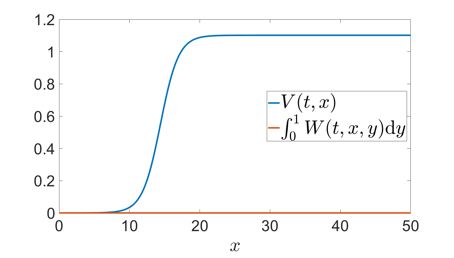
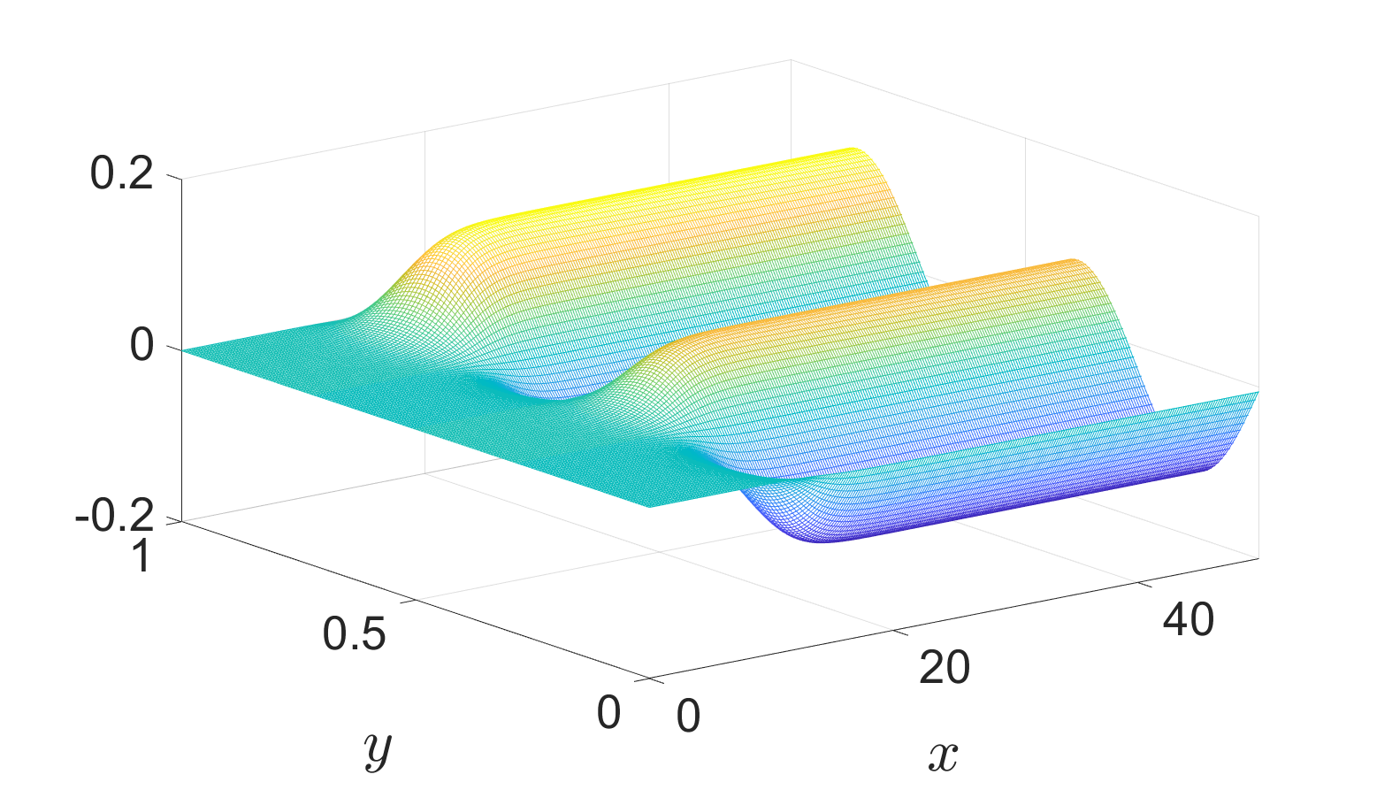
Figure 3.1: The front $(V,W)$ of the two-scale system (3.6) moves from right to left in $x$. Left: $V$ and average $\int_{\mathbb{T}}W(t,x,y)\;\!\mathrm{d}y$. Right: the $W(t,x,y)$-component in $(x,y)$-plane.

We can compare the solution $(V,W)$ of our two-scale limit system with the solution $(v_{\varepsilon},w_{\varepsilon})$ of the original system (3.4) with rapidly oscillating coefficients. In Figure 3.2 one can observe that the $\varepsilon$-periodic coupling coefficients induce $\varepsilon$-periodic oscillations of the solutions. Whereas the amplitude of the oscillations of the component $w_{\varepsilon}$ is of order $O(1)$, the postive diffusion $D_{\mathrm{v}}$ reduces the amplitude of the oscillations of the component $v_{\varepsilon}$ to order $O(\varepsilon)$, such that it vanishes in the limit $\varepsilon\to 0$. Notice that the component $w_{\varepsilon}$ also changes sign. Overall, the effective behavior of the oscillating solution $(v_{\varepsilon},w_{\varepsilon})$ is nicely captured by the two-scale limit $(V,W)$.

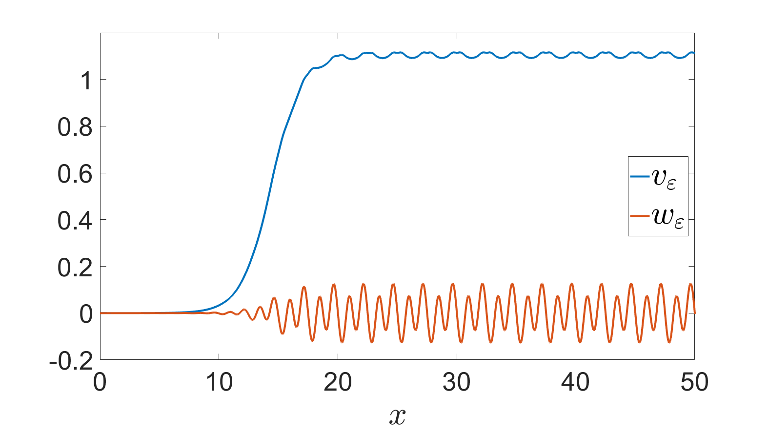
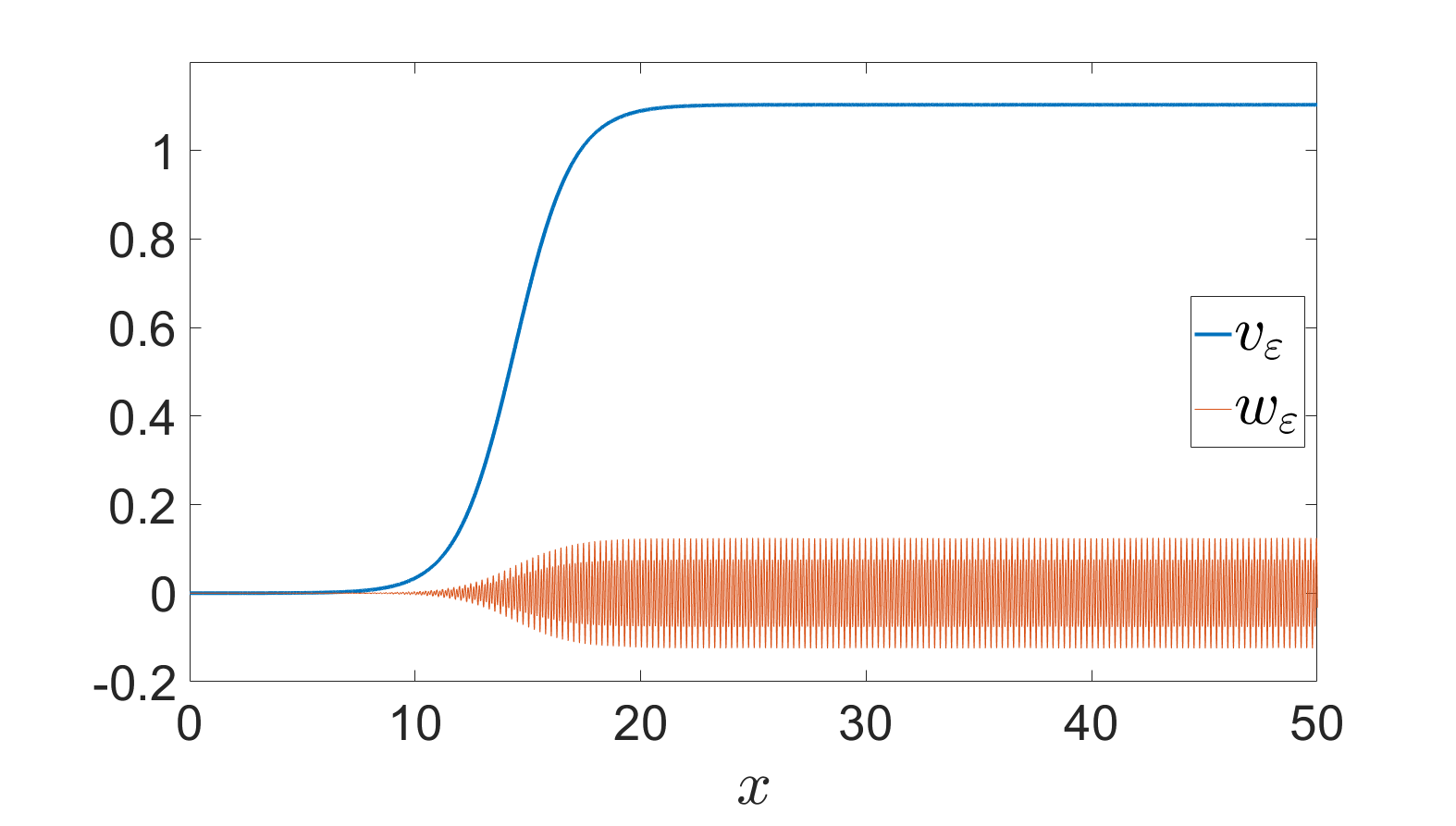
Figure 3.2: Solutions $(v_{\varepsilon},w_{\varepsilon})$ of the original system (3.4): left $\varepsilon{=}2.5$, right $\varepsilon{=}0.25$.

3.5 Possible generalizations

For mathematical conciseness we have decided to restrict ourselves to memory terms with a simple linear structure. However, as our theory is many based on the quite general work in [Che97] it is clear that the results can be generalized in several ways.

First, the integral memory can be replaced by discrete time delays in the form such that the equation reads

$$\dot{u}(t,x)=Du_{xx}(t,x)+F(u(t,x))+\sum_{j=1}^{j_{*}}\gamma_{j}u(t{-}\tau_{j},x).$$ (3.8)

Assuming $\gamma_{j}>0$ and setting $\gamma=\sum_{j=1}^{j_{*}}\gamma_{j}$, we obtain the memory equation (2.1) with a $\Gamma(\tau)=\sum_{j=1}^{j_{*}}\frac{\gamma_{j}}{\gamma}\,\delta_{\tau_{j}}(\tau)$. We refer to [WuZ01] for a general approach to traveling waves in reaction-diffusion equations involving linear and nonlinear delay terms.

Secondly, further generalizations can be obtained by looking at nonlinear couplings to ODEs, thus generalizing the coupled system (3.1):

$$\dot{u}=Du_{xx}+F(u)+\sum_{i=1}^{m_{\mathrm{w}}}A_{i}(u,w_{i}),\qquad\dot{w}_{i}=-\lambda_{i}w_{i}+B_{i}(u),$$ (3.9)

where the coupling functions $A_{i}:{\mathbb{R}}^{2}\to{\mathbb{R}}$ and $B_{i}:{\mathbb{R}}\to{\mathbb{R}}$ are assumed to be smooth functions with derivatives satisfying $\partial_{u}A(u,w_{i})\leq 0$, $\partial_{w_{i}}A_{i}(u,w_{i})\geq 0$, and $B^{\prime}_{i}(u)\geq 0$. Again we can express $w_{i}(t,x)$ as memory functional depending on $u(s,x)$ for $s\in{]{-}\infty,t[}$. Hence, (3.9) can be written in the form

$$\dot{u}(t,x)=Du_{xx}(t,x)+F(u(t,x))+\sum_{i=1}^{m_{\mathrm{w}}}A_{i}\big{(}u(t,x),{\mathrm{I}}\Gamma_{i}{*}B_{i}(u(\cdot,x))(t)\big{)},$$

$$\text{where }{\mathrm{I}}\Gamma_{i}{*}h(t)=\int_{0}^{\infty}\mathrm{e}^{-\lambda_{i}\tau}h(t{-}\tau)\;\!\mathrm{d}\tau.$$

Hence we have a memory in time, which is local in the space variable $x\in{\mathbb{R}}$. As in Section 2.2 we can introduce an auxiliary wave speed $\mathtt{v}$ and turn the memory terms into spatially nonlocal terms. Because of our assumptions on $A_{i}$ and $B_{i}$ we are exactly in the setting of [Che97, Eqn. (1.14)]. Thus, it is expected that the methods developed here can be extended to such nonlinear couplings.

Thirdly, it seems possible to generalize the theory to handle multidimensional traveling waves in a cylindrical domain $\Omega={\mathbb{R}}{\times}\Sigma$ as in [Gar86], but now with memory terms.

$$\dot{u}(t,x,y) =D\big{(}u_{xx}(t,x,y)+\Delta_{y}u(t,x,y)\big{)}$$

$$\quad+F(y,u(t,x,y))+\gamma\int_{0}^{\infty}\Gamma(\tau)u(t{-}\tau,x,y)\;\!\mathrm{d}\tau \text{for }t>0,\ (x,y)\in{\mathbb{R}}{\times}\Sigma,$$

$$0 =u(t,x,y) \text{for }t>0,\ (x,y)\in{\mathbb{R}}{\times}\partial\Sigma.$$

However, then the “bistability” Hypothesis (H1) has to be formulated in terms of the elliptic problem $u\mapsto D\Delta_{y}u+F(u)+\gamma u$ in $\Sigma$, which should have exactly three solutions $u^{\gamma}_{\alpha}\in{\mathrm{H}}^{1}_{0}(\Sigma)$ with appropriate properties.

4 Applications to the cubic case

In this section we study the classical FitzHugh-Nagumo system with a bistable cubic nonlinearity, namely

$$\dot{u}=u_{xx}+F(u)-\beta v,\qquad\dot{v}=-v+u,\quad F(u)=-u(u{-}a)(u{-}1),$$ (4.1)

where $a\in{]0,1[}$. Concerning traveling fronts, this system is equivalent to the memory equation

$$\dot{u}(t,x)=u_{xx}(t,x)+F(u(t,x))-\beta\int_{0}^{\infty}\mathrm{e}^{-\tau}u(t{-}\tau,x)\;\!\mathrm{d}\tau.$$ (4.2)

In particular, we see that the previous parameter $\gamma$ is given by $\gamma=-\beta$, such that our theory developed above only applies for $\beta\leq 0$. However, in the numerical simulations documented below, we are free to choose $\beta>0$ as well.

We first observe that the nonlinearity

$$F_{-\beta}(u)=-u(u{-}a)(u{-}1)-\beta u$$

has a bistable structure if and only if $\beta<(1{-}a)^{2}/4$ and then

$$u^{-\beta}_{-}=0,\quad u^{-\beta}_{\mathrm{m}}=\frac{1{+}a}{2}-\frac{1}{2}\sqrt{(1{-}a)^{2}-4\beta},\quad u^{-\beta}_{+}=\frac{1{+}a}{2}+\frac{1}{2}\sqrt{(1{-}a)^{2}-4\beta}.$$

In [McK70], the wave speed of the local model $\dot{u}=u_{xx}+F_{-\beta}(u)$ is calculated explicitly, which gives

$$\mathtt{C}^{\mathrm{FN}}(-\beta,0):=\frac{1}{\sqrt{2}}\big{(}2u^{-\beta}_{\mathrm{m}}-u^{-\beta}_{+}\big{)}=\frac{1}{2\sqrt{2}}\Big{(}1{+}a-3\sqrt{(1{-}a)^{2}-4\beta}\>\Big{)}.$$

In the case $\beta=0$ there is no coupling between the ODE an the PDE, hence $\mathtt{c}_{0}=\mathtt{C}^{\mathrm{FN}}(0,0)=(2a{-}1)/{\sqrt{2}}$ is known.

In the case $a\in{]\frac{1}{2},1[}$, which we fix from now on, the function $\beta\mapsto\mathtt{C}({-}\beta,0)$ changes sign at

$$\beta_{0}(a)=\tfrac{1}{9}\big{(}2a^{2}{-}5a{+}2\big{)}\in{]{-}\tfrac{1}{9},0[}.$$

With $\mathtt{C}^{\mathrm{FN}}(0,0)=(2a{-}1)/{\sqrt{2}}>0$, we obtain $\mathtt{C}^{\mathrm{FN}}(-\beta,0)>0$ for $\beta\in{]\beta_{0}(a),\frac{1}{4}(1{-}a)^{2}]}$ and $\mathtt{C}^{\mathrm{FN}}(-\beta,0)<0$ for $\beta<\beta_{0}(a)$.

From this, we see that we can apply our existence theory in Theorem 2.8 and obtain a unique traveling front for the FitzHugh-Nagumo (4.1), or equivalently for the memory equation (4.2) for all $\beta\leq 0$. This front connects the values $u^{-\beta}_{-}=0$ and $u^{-\beta}_{+}$, and using Corollary 2.9 it travels with the speed $\mathtt{c}_{-\beta}$ satisfying the bound

$$0\leq\mathtt{c}_{-\beta}\leq\mathtt{C}^{\mathrm{FN}}({-}\beta,0) \quad\text{for }\beta\in[\beta_{0}(a),0],$$

$$\mathtt{C}^{\mathrm{FN}}({-}\beta,0)\leq\mathtt{c}_{-\beta}\leq 0 \quad\text{for }\beta\leq\beta_{0}(a).$$

For numerical simulations we choose $a=0.6$ determine $\mathtt{c}_{-\beta}$ on the whole bistable regime $\beta\leq(1{-}a)^{2}/4=0.04$. For this case, we have $\mathtt{c}_{0}=\mathtt{C}^{\mathrm{FN}}(0,0)=0.2/\sqrt{2}\approx 0.1414$ and

$$\mathtt{C}^{\mathrm{FN}}(-\beta,0)=\frac{1}{2\sqrt{2}}\big{(}1.6-3\sqrt{0.4^{2}-4\beta}\>\big{)}\approx 0.566-2.12\sqrt{0.04{-}\beta}$$

as upper or lower bound for $\mathtt{c}_{-\beta}$. Moreover, we know that $\mathtt{C}^{\mathrm{FN}}({-}\beta,0)$ changes sign at $\beta_{0}(0.6)=-0.28/9\approx-0.0311$.

To determine the speed of the traveling front numerically, we solve the coupled system (4.1) starting from front-like initial data with the correct plateau $(u,v)=(u^{-\beta}_{+},u^{-\beta}_{+})$ for large $x$ and $(u,v)=(0,0)$ for small $x$. The solution rapidly stabilizes into the front and the speed $\mathtt{c}_{-\beta}$ can be measured. The numerical simulations nicely confirm the bounds on the wave speed $\mathtt{c}_{-\beta}$ in Corollary 2.9. For all $\beta<\beta_{0}(0.6)\approx-0.0311$, Figure 4.1 shows $\mathtt{C}(-\beta,0)\leq\mathtt{c}_{-\beta}\leq 0$.

Figure 4.1: The region $\beta\in[-5,-0.03]$ was sampled with $\beta$-steps of size $0.01$ to find $\mathtt{c}_{-\beta}\in[\mathtt{C}^{\mathrm{FN}}(-\beta,0),0]$.

For $\beta\in[\beta_{0}(0.6),0]$ Figure 4.2 shows $0\leq\mathtt{c}_{-\beta}\leq\mathtt{C}(-\beta,0)$ as predicted by the theory. For positive $\beta\in{]0,0.04[}$ Theorem 2.8 does not apply, however, the comparison argument in (2.17) predicts the reverse relation $\mathtt{c}_{-\beta}\geq\mathtt{C}(-\beta,0)\geq 0$, which is confirmed in the simulations, which also show that $\mathtt{c}_{-\beta}$ and $\mathtt{C}(-\beta,0)$ only differ less than a percent in relative size for all $\beta\in[-0.06,0.03]$. Moreover, the identities $\mathtt{c}_{-\beta}=\mathtt{C}(-\beta,0)$ are confirmed for $\beta=\beta_{0}(0.6)$ and $\beta=0$.

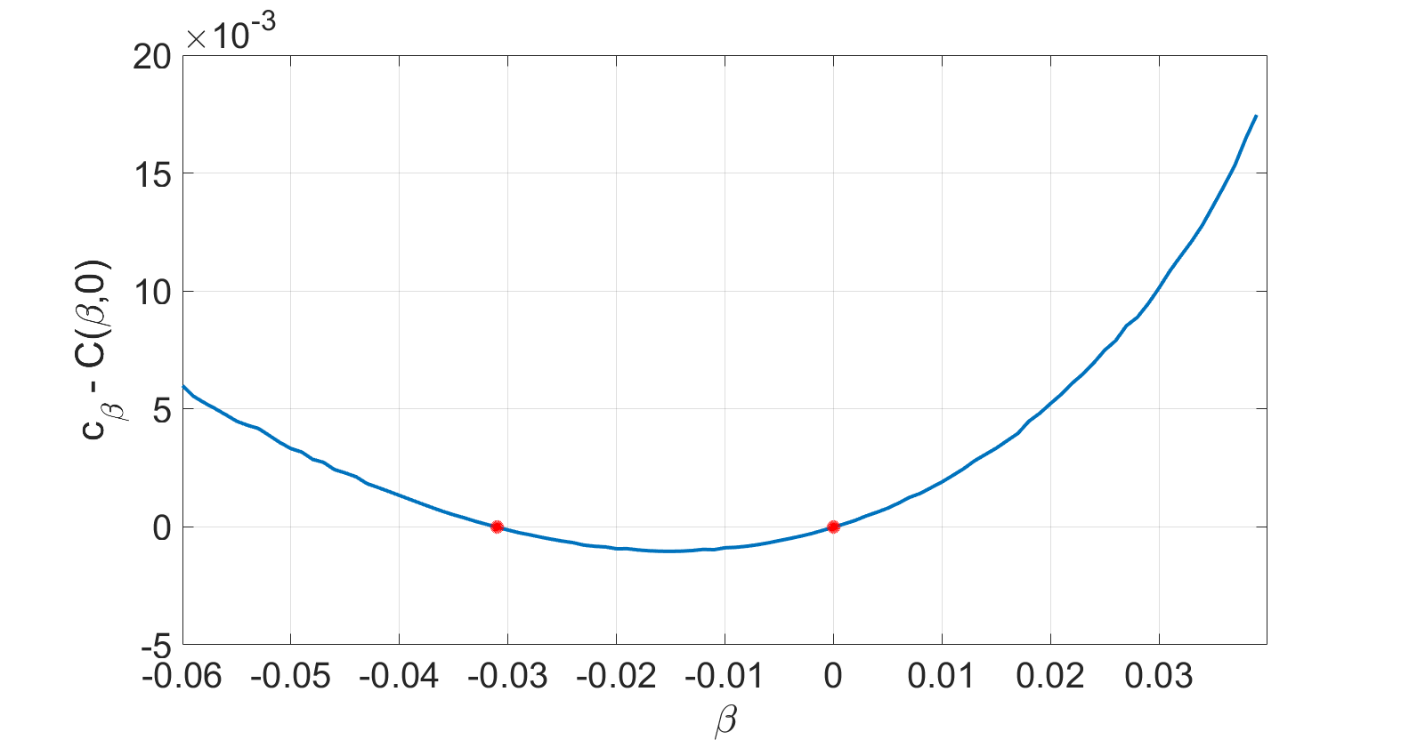
Figure 4.2: The region $\beta\in[-0.06,0.04]$ was sampled with $\beta$-steps of size $0.001$ to compare $\mathtt{c}_{-\beta}$ and $\mathtt{C}(-\beta,0)$ in the upper figure. As the two graphs differ only little, the lower figure displays $c_{-\beta}-\mathtt{C}(-\beta,0)$, where the sign changes at $\beta=\beta_{0}(0.6)\approx-0.0311$ and $\beta=0$ are clearly visible.

Appendix A Two-scale convergence in weighted Sobolev spaces

The aim of this appendix is to explain how the result in Theorem 3.1 for $\Omega={\mathbb{R}}^{d}$ can be derived by generalizing the theory for bounded Lipschitz domains $\Omega\subset{\mathbb{R}}^{d}$ as developed in [MRT14, Rei15]. To this end we introduce a few notations from two-scale convergence and two-scale homogenization as developed in [Ngu89, All92, MiT07, CDG08]. For arbitrary (bounded or unbounded) Lipschitz domains $\Omega\subseteq{\mathbb{R}}^{d}$, we set

$${\mathcal{T}}_{\varepsilon}:{\mathrm{L}}^{2}(\Omega)\to{\mathrm{L}}^{2}({\mathbb{R}}^{d}{\times}{\mathbb{T}}^{d});\quad({\mathcal{T}}_{\varepsilon}u)(x,y):=u_{\mathrm{ex}}\left(\varepsilon\left[\tfrac{x}{\varepsilon}\right]+\varepsilon y\right),$$

where $u_{\mathrm{ex}}\in{\mathrm{L}}^{2}({\mathbb{R}}^{d})$ is obtained by extension with $0$ on ${\mathbb{R}}^{d}\backslash\Omega$ and $[z]\in{\mathbb{Z}}^{d}$ denotes the integer part for any $z\in{\mathbb{R}}^{d}$. We define weak and strong two-scale convergence via

$$u_{\varepsilon}\operatorname{\ext@arrow 0359{\arrowfill@\relbar\relbar\rightharpoonup}{}{2w}}U\text{ in }{\mathrm{L}}^{2}(\Omega{\times}{\mathbb{T}}^{d}) \quad:\overset{\text{Def.}}{\Longleftrightarrow}\quad{\mathcal{T}}_{\varepsilon}u_{\varepsilon}\rightharpoonup U_{\mathrm{ex}}\text{ in }{\mathrm{L}}^{2}({\mathbb{R}}^{d}{\times}{\mathbb{T}}^{d}),$$

$$u_{\varepsilon}\operatorname{\xrightarrow{2s}}U\text{ in }{\mathrm{L}}^{2}(\Omega{\times}{\mathbb{T}}^{d}) \quad:\overset{\text{Def.}}{\Longleftrightarrow}\quad{\mathcal{T}}_{\varepsilon}u_{\varepsilon}\to U_{\mathrm{ex}}\text{ in }{\mathrm{L}}^{2}({\mathbb{R}}^{d}{\times}{\mathbb{T}}^{d}).$$

We briefly recall the mathematical setting for the $\varepsilon$-problem (3.3) such that the two-scale system (3.4) is rigorously justified. The fourth order diffusion tensors ${\mathbb{D}}_{i}\in\mathrm{Lin}({\mathbb{R}}^{d{\times}m_{i}};{\mathbb{R}}^{d{\times}m_{i}})$ are uniformly elliptic and bounded, i.e. there exist constants $M,\mu>0$ such that

$${\mathbb{D}}_{\mathrm{i}}(y)\xi:\xi\geq\mu|\xi|^{2}\quad\text{and}\quad|{\mathbb{D}}_{\mathrm{i}}(y)\xi|\leq M|\xi|\quad\text{for all }\xi\in{\mathbb{R}}^{d{\times}m_{\mathrm{i}}}\text{ and }{\mathrm{i}}\in\{{\mathrm{v}},{\mathrm{w}}\},$$

and they are not necessarily symmetric. For the reaction terms we assume boundedness $f_{\mathrm{i}}(\cdot,v,w)\in{\mathrm{L}}^{\infty}({\mathbb{T}}^{d})$ and global Lipschitz continuity, i.e. there exists $L>0$ such that for $v_{1},v_{2}\in{\mathbb{R}}^{m_{\mathrm{v}}}$ and $w_{1},w_{2}\in{\mathbb{R}}^{m_{\mathrm{w}}}$

$$|f_{\mathrm{i}}(y,v_{1},w_{1})-f_{\mathrm{i}}(y,v_{2},w_{2})|\leq L(|v_{1}{-}v_{2}|+|w_{1}{-}w_{2}|)\quad\text{for }{\mathrm{i}}\in\{{\mathrm{v}},{\mathrm{w}}\}.$$

In addition to the weighted Lebesgue spaces ${\mathrm{L}}^{2}_{\varrho}({\mathbb{R}}^{d})$ and ${\mathrm{L}}^{2}_{\varrho}({\mathbb{R}}^{d}{\times}{\mathbb{T}}^{d})$ from (3.5), we also define the weighted Sobolev spaces ${\mathrm{H}}^{1}_{\varrho}({\mathbb{R}}^{d})$ and ${\mathrm{L}}^{2}_{\varrho}({\mathbb{R}}^{d};{\mathrm{H}}^{1}({\mathbb{T}}^{d}))$ via

$${\mathrm{H}}^{1}_{\varrho}({\mathbb{R}}^{d}) :=\Big{\{}\>u\in{\mathrm{H}}^{1}_{\mathrm{loc}}({\mathbb{R}}^{d})\;\Big{|}\;\|u\|_{{\mathrm{L}}^{2}_{\varrho}({\mathbb{R}}^{d})}+\|\nabla u\|_{{\mathrm{L}}^{2}_{\varrho}({\mathbb{R}}^{d})}<\infty\>\Big{\}},$$

$${\mathrm{L}}^{2}_{\varrho}({\mathbb{R}}^{d};{\mathrm{H}}^{1}({\mathbb{T}}^{d})) :=\Big{\{}\>U\in{\mathrm{L}}^{2}_{\mathrm{loc}}({\mathbb{R}}^{d};{\mathrm{H}}^{1}({\mathbb{T}}^{d}))\;\Big{|}\;\|U\|_{{\mathrm{L}}^{2}_{\varrho}({\mathbb{R}}^{d}{\times}{\mathbb{T}}^{d})}+\|\nabla_{y}U\|_{{\mathrm{L}}^{2}_{\varrho}({\mathbb{R}}^{d}{\times}{\mathbb{T}}^{d})}<\infty\>\Big{\}}.$$

Our choice $\varrho(x)=1/\cosh(|x|/R)$ gives $\varrho,\varrho^{-1}\in{\mathrm{L}}^{1}_{\mathrm{loc}}({\mathbb{R}}^{d})$, which implies that the weighted Lebesgue and Sobolev spaces are Banach spaces, see e.g. [GoU09, Thm. 1]. Moreover, introducing the scalar product $(u,v)_{{\mathrm{L}}^{2}_{\varrho}({\mathbb{R}}^{d})}:=(\sqrt{\varrho}u,\sqrt{\varrho}v)_{{\mathrm{L}}^{2}({\mathbb{R}}^{d})}$ yields that they are also separable Hilbert spaces. The proof of Theorem 3.1 follows along the lines of [MRT14, Thm. 4.1] and [Rei15, Thm. 2.1.1, Thm. 2.2.1] with the following modifications.

• The definition of the periodic unfolding operator

  $${\mathcal{T}}_{\varepsilon}:{\mathrm{L}}^{2}_{\varrho}({\mathbb{R}}^{d})\to{\mathrm{L}}^{2}_{\varrho}({\mathbb{R}}^{d}{\times}{\mathbb{T}}^{d});\quad({\mathcal{T}}_{\varepsilon}u)(x,y):=u\left(\varepsilon\left[\tfrac{x}{\varepsilon}\right]+\varepsilon y\right)$$

  is immediate and the notion of two-scale convergence follows analogously. Notice that the assumptions on the weight function imply the unfolding estimate

  $$\|{\mathcal{T}}_{\varepsilon}\varrho-\varrho\|_{{\mathrm{L}}^{\infty}({\mathbb{R}}^{d}{\times}{\mathbb{T}}^{d})}\leq\varepsilon\sqrt{d}\|\nabla\varrho\|_{{\mathrm{L}}^{\infty}({\mathbb{R}}^{d})}\leq\varepsilon\sqrt{d}/R.$$

  Hence, we obtain the upper bound for unfolded functions $u\in{\mathrm{L}}^{2}_{\varrho}({\mathbb{R}}^{d})$

  $$\|{\mathcal{T}}_{\varepsilon}u\|_{{\mathrm{L}}^{2}_{\varrho}({\mathbb{R}}^{d}{\times}{\mathbb{T}}^{d})}\leq U_{\varepsilon}\|u\|_{{\mathrm{L}}^{2}_{\varrho}({\mathbb{R}}^{d})}\quad\text{with}\quad U_{\varepsilon}=\big{(}1-\varepsilon\sqrt{d}/R\big{)}^{-1/2}.$$

• The standard compactness results for two-scale convergence [Ngu89, All92, MiT07] also hold for weighted spaces, since they are, in particular, separable Banach spaces and the Banach–Alaoglu Theorem is applicable.

• The definition of the gradient folding operator $\mathcal{G}^{\mathrm{slow}}_{\varepsilon}$ (cf. [MRT14, Def. 3.5]) needs to be adapted as follows: In the case of slow diffusion of order $O(\varepsilon^{2})$, we define for $W\in{\mathrm{L}}^{2}_{\varrho}({\mathbb{R}}^{d};{\mathrm{H}}^{1}({\mathbb{T}}^{d}))$ the one-scale function $\mathcal{G}^{\mathrm{slow}}_{\varepsilon}W:=\hat{w}_{\varepsilon}\in{\mathrm{H}}^{1}_{\varrho}({\mathbb{R}}^{d})$, which is given by the Lax–Milgram lemma as the unique solution of the elliptic problem

  $$\int_{{\mathbb{R}}^{d}}\big{[}\sqrt{\varrho}\hat{w}_{\varepsilon}-\mathcal{F}_{\varepsilon}\left(\sqrt{\varrho}W\right)\big{]}\cdot\sqrt{\varrho}\varphi+\big{[}\varepsilon\sqrt{\varrho}\nabla\hat{w}_{\varepsilon}-\mathcal{F}_{\varepsilon}\left(\sqrt{\varrho}\nabla_{y}W\right)\big{]}:\varepsilon\sqrt{\varrho}\nabla\varphi\;\!\mathrm{d}x=0$$

  for all $\varphi\in{\mathrm{H}}^{1}_{\varrho}({\mathbb{R}}^{d})$.

• For the slowly diffusing species $w_{\varepsilon}$, we choose the test function $\varphi^{\mathrm{slow}}_{\varepsilon}=\varrho\left(w_{\varepsilon}{-}\mathcal{G}^{\mathrm{slow}}_{\varepsilon}W\right)$ and continue as in [MRT14, Rei15]. For species $v_{\varepsilon}$ undergoing diffusion of order $O(1)$, we proceed analogously (cf. [Rei15, Def. 1.2.7]) and choose the test function $\varphi^{\mathrm{stand}}_{\varepsilon}=\varrho\left(v_{\varepsilon}-\mathcal{G}^{\mathrm{stand}}_{\varepsilon}V\right)$.

With these modifications for $\Omega={\mathbb{R}}^{d}$, the proofs in [MRT14, Thm. 4.1] and [Rei15, Thm. 2.1.1, Thm. 2.2.1] can be easily adapted, and the proof of Theorem 3.1 is complete.

Acknowledgments.

The authors are grateful to Christian Kühn for illuminating discussions and to Stefanie Schindler for many helpful comments. This research was supported by Deutsche Forschungsgemeinschaft through the Collaborative Research Center SFB 910 Control of self-organizing nonlinear systems (Project no. 163436311) via the subproject A5 “Pattern formation in coupled parabolic systems”.

References

- [AcK15] F. Achleitner and C. Kuehn. Traveling waves for a bistable equation with nonlocal diffusion. Adv. Diff. Eqns., 20(9-10), 887–936, 2015.
- [All92] G. Allaire. Homogenization and two-scale convergence. SIAM J. Math. Anal., 23, 1482–1518, 1992.
- [BeH02] H. Berestycki and F. Hamel. Front propagation in periodic excitable media. Comm. Pure Appl. Math., 55(8), 949–1032, 2002.
- [BLP78] A. Bensoussan, J.-L. Lions, and G. Papanicolaou. Asymptotic analysis for periodic structures, volume 5 of Studies in Mathematics and its Applications. North-Holland Publishing Co., Amsterdam, 1978.
- [BoM14] A. Boden and K. Matthies. Existence and homogenisation of travelling waves bifurcating from resonances of reaction-diffusion equations in periodic media. J. Dynam. Differential Equations, 26(3), 405–459, 2014.
- [Car77] G. A. Carpenter. A geometric approach to singular perturbation problems with applications to nerve impulse equations. J. Diff. Eqns., 23(3), 335–367, 1977.
- [CDG08] D. Cioranescu, A. Damlamian, and G. Griso. The periodic unfolding method in homogenization. SIAM J. Math. Anal., 40(4), 1585–1620, 2008.
- [CGW08] X. Chen, J.-S. Guo, and C.-C. Wu. Traveling waves in discrete periodic media for bistable dynamics. Arch. Rational Mech. Anal., 189(2), 189–236, 2008.
- [Che97] X. Chen. Existence, uniqueness, and asymptotic stability of traveling waves in nonlocal evolution equations. Adv. Differential Equations, 2(1), 125–160, 1997.
- [Den91] B. Deng. The existence of infinitely many traveling front and back waves in the FitzHugh-Nagumo equations. SIAM J. Math. Analysis, 22(6), 1631–1650, 1991.
- [Eva98] L. C. Evans. Partial differential equations, volume 19 of Graduate Studies in Mathematics. American Mathematical Society, Providence, RI, 1998.
- [FiM77] P. C. Fife and J. B. McLeod. The approach of solutions of nonlinear diffusion equations to travelling front solutions. Arch. Rational Mech. Anal., 65, 335–361, 1977.
- [Gar86] R. Gardner. Existence of multidimensional travelling wave solutions of an initial-boundary value problem. J. Diff. Eqns., 61, 335–379, 1986.
- [GoU09] V. Gol’dshtein and A. Ukhlov. Weighted Sobolev spaces and embedding theorems. Trans. Amer. Math. Soc., 361(7), 3829–3850, 2009.
- [GuH06] J.-S. Guo and F. Hamel. Front propagation for discrete periodic monostable equations. Math. Ann., 335(3), 489–525, 2006.
- [GuR18] P. Gurevich and S. Reichelt. Pulses in FitzHugh–Nagumo systems with rapidly oscillating coefficients. Multiscale Model. Simul., 16(2), 833–856, 2018.
- [Hei01] S. Heinze. Wave solutions to reaction-diffusion systems in perforated domains. Zeits. Analysis Anwend., 20(3), 661–676, 2001.
- [HuZ95] W. Hudson and B. Zinner. Existence of traveling waves for reaction diffusion equations of Fisher type in periodic media. In Boundary value problems for functional-differential equations, pages 187–199. World Sci. Publ., River Edge, NJ, 1995.
- [McK70] H. McKean Jr. Nagumo’s equation. Advances in Math., 4(3), 1970.
- [MiT07] A. Mielke and A. M. Timofte. Two-scale homogenization for evolutionary variational inequalities via the energetic formulation. SIAM J. Math. Analysis, 39(2), 642–668, 2007.
- [MRT14] A. Mielke, S. Reichelt, and M. Thomas. Two-scale homogenization of nonlinear reaction-diffusion systems with slow diffusion. Networks Heterg. Materials, 9(2), 353–382, 2014.
- [MSU07] K. Matthies, G. Schneider, and H. Uecker. Exponential averaging for traveling wave solutions in rapidly varying periodic media. Math. Nachr., 280(4), 408–422, 2007.
- [NAY62] J. Nagumo, S. Arimoto, and S. Yoshizawa. An active pulse transmission line simulating nerve axon. Proc. Inst. Radio Eng., 50(10), 2061–2070, 1962.
- [Ngu89] G. Nguetseng. A general convergence result for a functional related to the theory of homogenization. SIAM J. Math. Anal., 20(3), 608–623, 1989.
- [Rei15] S. Reichelt. Two-scale homogenization of systems of nonlinear parabolic equations. PhD thesis, Institut für Mathematik, Humboldt-Universität zu Berlin, November 2015.
- [WuZ01] J. Wu and X. Zou. Traveling wave fronts of reaction-diffusion systems with delay. J. Dynam. Differential Equations, 13(3), 651–687, 2001.
- [Xin00] J. Xin. Front propagation in heterogeneous media. SIAM Review, 42(2), 161–230, 2000.