Algorithms for ridge estimation with convergence guarantees

Abstract

The extraction of filamentary structure from a point cloud is discussed. The filaments are modeled as ridge lines or higher dimensional ridges of an underlying density. We propose two novel algorithms, and provide theoretical guarantees for their convergences. We consider the new algorithms as alternatives to the Subspace Constraint Mean Shift (SCMS) algorithm that do not suffer from a shortcoming of the SCMS that is also revealed in this paper.

Keywords: Filaments, Ridges, Manifold Learning, Mean Shift, Gradient Ascent

1 Introduction

The geometric interpretation of a ridge in $\mathbb{R}^{d}$ is that of a low-dimensional structure along which the density is higher than in the surrounding area when moving away from the set in an orthogonal direction. Blood vessels, road system, DNA strands or fault lines appearing in 2D or 3D images can be modeled as filaments, or maybe better as unions of filaments that might intersect, or that have a common starting point. We sometimes call such unions filamentary structures. Another example is provided by the filamentary structure that can be observed in the distribution of galaxies in the universe, the ‘cosmic web’. Cosmologists are interested in finding rigorous geometric and topological descriptions of the filamentary structures. Usually, the first step is the extraction of this structure, and this is the topic discussed below.

Ozertem and Erdogmus (2011) developed the popular SCMS (Subspace Constrained Mean Shift) algorithm for extracting estimates of $k$-dimensional ridges of a $d$-dimensional density $f$ from a point cloud sampled from $f$. The algorithm consists in running a corrected mean shift algorithm (subspace constrained) starting at a data point. For each data point the algorithm then provides an estimate of a point on the ridge. While the algorithm works well in practice, we here reveal a shortcoming of the algorithm: Some parts of the ridges might be missed by the algorithm. This is discussed below in some detail (see subsection 2.3).

Here we propose algorithms that does not suffer from the shortcoming of the SCMS algorithm just mentioned, and we also derive theoretical guarantees for their convergence. So far, no theoretical guarantees for the SCMS algorithm seem to be known.

The heuristic underlying our algorithm is simple: Consider a one-dimensional ridge line of a smooth density $f$. A point $x$ on the ridge line is characterized by the conditions (i) $V^{\top}_{\perp}(x)\nabla f(x)={\bf 0}$ and (ii) $\lambda_{i}(x)<0,\,i=2,\ldots,d$. Here ${\bf 0}$ is the zero-vector in $\mathbb{R}^{d-1}$, $\lambda_{i}(x)$ are the eigenvalues of the Hessian of $f$ at $x$, $\nabla f(x)$ denotes the gradient of $f$, and the columns of the $(d\times(d-1))$-matrix $V_{\perp}$ are the orthonormal eigenvectors of the Hessian of $f$ corresponding to $\lambda_{2},\ldots,\lambda_{d}.$ Observing that (i) is equivalent to $\|V^{\top}_{\perp}(x)\nabla f(x)\|^{2}=0$, we can find ridge points by finding the global minimizers of the real-valued function $r(x)=\|V^{\top}_{\perp}(x)\nabla f(x)\|^{2}$ subject to (ii). Given data $X_{1},\ldots,X_{n}$ sampled from $f$, one can simply replace all the population quantities by the ones corresponding to a KDE (kernel density estimator) of $f.$ We will devise subspace-constrained type algorithms for finding the entire set of global minimizers of the function $r$ subject to condition (ii), i.e., the ridge lines, and of higher-dimensional analogs.

The literature on ridge (or filament) detection is rich, and different approaches use different geometric ideas. For instance, Qiao and Polonik (2016) use the fact that integral curves driven by the second eigenvectors of the Hessians of the density $f$ can be used to extract ridges. Other approaches include the skeleton (Novikov et al. 2006), local principal curves (Einbeck et al. 2005, 2007), minimum spanning trees (Barrow et al. 1985), the candy model (Stoica et al. 2007), multiscale detection (Arias-Castro et al. 2006) and the path density (Genovese et al. 2009). Other related concepts include principal curves (Hastie et al. 1989) and the medial axis (Genovese et al. 2012). Also see Chen et al. (2015), Pulkinnen (2015), and Qiao (2021).

The remaining part of the paper is organized as follows. In Section 2 we introduce the definition of ridges. This is followed by our extraction algorithm, which is illustrated using a few datasets in $\mathbb{R}^{2}$. The main results are given in Subsection 2.9, where we show the convergence of our algorithms. All the mathematical details are given in Section 3.

2 Extraction of filamentary structures

2.1 Definition

We use the following definition of a ridge (filament) as given in Eberly (1996).

Definition 1

(Ridge points in $\mathbb{R}^{d}$). Let $f:\mathbb{R}^{d}\mapsto\mathbb{R}$ be a twice differentiable density function on $\mathbb{R}^{d}$. Suppose the Hessian $\nabla^{2}f(x)$ has eigenvalues $\lambda_{1}(x)\geq\cdots\geq\lambda_{k}(x)>\lambda_{k+1}(x)\cdots\geq\lambda_{d}(x)$ with $V_{1}(x),\cdots,V_{d}(x)$ being the corresponding orthonormal eigenvectors. For $1\leq k\leq d-1$, a point $x$ is said to be a $k-$dimensional ridge point if

$$\left\langle\nabla f(x),V_{i}(x)\right\rangle =0,\;\;\text{for }\,i=k+1,\cdots,d,$$ (2.1)

and

$$\lambda_{k+1}(x) <0.$$ (2.2)

The geometric intuition underlying this definition is clear: Since the (first order) directional derivative of $f(x)$ along $V_{i}(x)$ is $\langle\nabla f(x),V_{i}(x)\rangle$ and the second order directional derivative of $f(x)$ along $V_{i}(x)$ is $\lambda_{i}(x)\|V_{i}(x)\|^{2}$, conditions (2.1) and (2.2) mean that the point $x$ is a local mode in the linear subspace spanned by $V_{i}(x),\;i=k+1,\cdots,d$, for which the density has the largest concavity (see Eberly, 1996).

Let $V_{\perp}=[V_{k+1},\cdots,V_{d}]\in{\mathbb{R}}^{d\times(d-k)}$. For a twice differentiable function $f$, a ridge is the set of ridge points, given by

$$\text{Ridge}(f)=\{x\in\mathbb{R}^{d}:\;V_{\perp}(x)^{\top}\nabla f(x)={\bf 0}\;\text{ and }\;\lambda_{k+1}(x)<0\}.$$

If we have an estimator $\widehat{f}$ for $f$, then $\text{Ridge}(\widehat{f}\,)$ is a plug-in estimator for $\text{Ridge}(f)$. In this work we consider $f$ to be a density function, and given an i.i.d. sample $X_{1},\cdots,X_{n}$ from $f$, we use a kernel density estimator $\widehat{f}$ of the form

$$\widehat{f}(x)=\frac{1}{nh^{d}}\sum_{i=1}^{n}K\left(\frac{X_{i}-x}{h}\right),$$

where $h>0$ is a bandwidth and $\int_{\mathbb{R}^{d}}K(u)du=1$. Denote the eigenvalues of the Hessian $\nabla^{2}\widehat{f}(x)$ by $\widehat{\lambda}_{1}(x)\geq\widehat{\lambda}_{2}(x)\geq\cdots\geq\widehat{\lambda}_{d}(x),$ and let $\widehat{V}_{1}(x),\cdots\widehat{V}_{d}(x)$ be the corresponding orthonormal eigenvectors. With $\widehat{V}_{\perp}=[\widehat{V}_{k+1},\cdots,\widehat{V}_{d}]$, we then have

$$\text{Ridge}(\widehat{f}\,)=\{x\in\mathbb{R}^{d}:\;\widehat{V}_{\perp}(x)^{\top}\nabla\widehat{f}(x)={\bf 0}\;\text{ and }\;\widehat{\lambda}_{k+1}(x)<0\}.$$

Of course, this only gives the definition of an estimated ridge. One still needs an algorithm to actually extract the estimated ridges from data.

2.2 Mean shift algorithm and subspace constrained mean shift algorithm

One of the popular algorithms for ridge extraction is called Subspace Constrained Mean Shift (SCMS), proposed in Ozertem and Erdogmus (2011). The algorithm uses the idea of mean shift, which is briefly reviewed first. The mean shift algorithm (Fukanaga and Hostetler, 1975) is essentially tracking non-parametric estimates of gradients. It is being used for mode finding and clustering, e.g. see Cheng (1995) and Comaniciu and Meer (1999, 2002). Considering the above kernel estimator with $K(x)=\phi(\|x\|)$, the vector

$$m(x):=\frac{\sum_{i=1}^{n}X_{i}\phi\big{(}\frac{\|x-X_{i}\|}{h}\big{)}}{\sum_{i=1}^{n}\phi\big{(}\frac{\|x-X_{i}\|}{h}\big{)}}-x$$ (2.3)

is called mean shift. It is well known that the direction of the mean shift is an estimator of the direction of the gradient of $f$ at $x$. Given some initial position $y_{0}$, let the points $y_{1},y_{2},\cdots$ be defined iteratively by

$$y_{j+1}=m(y_{j})+y_{j},\;\;j=0,1,2,\cdots.$$ (2.4)

Successively connecting these points provides an estimate of the integral curve driven by the gradient, starting from $y_{0}$. The endpoint of this iteration (after applying some stopping criterion) is considered to be an estimate of a mode of $f$. This is the popular mean shift algorithm.

The idea of using a subspace constraint comes in when the target is a ridge. To this end, one modifies the just described hill climbing algorithm by following the direction of the gradient projected on the subspace spanned by the eigenvectors of the Hessian corresponding to small eigenvalues, thereby exploiting the definition of a ridge point. In this algorithm, the gradient direction is approximated by the mean shift and the Hessian is estimated by the Hessian of the kernel density estimator. More specifically, given a starting point $y_{0}$, the SCMS generates a sequence

$$y_{j+1}=\widehat{V}_{\perp}(y_{j})\widehat{V}_{\perp}(y_{j})^{\top}m(y_{j})+y_{j},\quad j=0,1,2,\ldots$$ (2.5)

where $m(y)$ is the mean shift vector, and $\widehat{V}_{\perp}(y)\widehat{V}_{\perp}^{\top}(y)$ is the projection matrix onto the subspace spanned by the trailing $(d-k)$ eigenvectors of the estimated Hessian evaluated at $y$. Notice that for $y\in{\rm Ridge}(\widehat{f}\,)$, this space is orthogonal to the ridge (see below for more). This motivates that the endpoint of this iteration (after applying some stopping criterion) is considered to be an estimated ridge point. The SCMS algorithm is very popular, and it gives nice results in practice.

2.3 A shortcoming of the SCMS Algorithm

The main idea behind SCMS is to consider ridge points as local maxima on the trajectories along the tangent direction of $V_{\perp}V_{\perp}^{\top}\nabla f$, the projection of $\nabla f$ onto the subspace spanned by the $(d-k)$ trailing eigenvectors of $\nabla^{2}f$. This is the ascending direction that SCMS tries to estimate. Indeed, a ridge point $x_{0}$ is a local mode in the direction given by the columns of $V_{\perp}(x_{0})$. In other words, a ridge point $x_{0}$ is a local mode in the linear subspace $\{x_{0}+V_{\perp}(x_{0})^{\top}t:\;t\in\mathbb{R}^{d-k}\}$. This is because for $i=1,\cdots,n$, the sign of $\lambda_{i}(x_{0})$ determines the sign of the second order directional derivative in the direction of $V_{i}(x_{0})$, assuming that the eigenvalues are simple, i.e., without ties, that is,

$$\nabla_{V_{i}(x_{0})}\left(\nabla_{V_{i}(x_{0})}f(x)\right)=\lambda_{i}(x_{0})\|{V_{i}(x_{0})}\|^{2},$$ (2.6)

where $\nabla_{V_{i}(x_{0})}$ is the directional derivative along $V_{i}(x_{0})$. Thus, the ridge point $x_{0}$ yielding a local maximum of $f$ in the directions of $V_{i}(x_{0}),i=k+1,\ldots,d$ follows from the condition in (2.1) that $\lambda_{i}(x_{0})<0$ for $i=k+1,\ldots,d,$ and the first order condition in (2.1). However, when running the SCMS algorithm, we of course do not know which point is a ridge point. Therefore, at a given step of the algorithm, we project the gradient at the current point $y_{j}$, say, on the space spanned by $\{V_{i}(y_{j}),i=k+1,\cdots,d\}$. Implicitly this means that we view the $V_{i}$’s as functions of $x$, and in this case, the derivatives are taken constrained in the corresponding integral surface, and because of this, the signs of the directional derivatives are usually not determined by the signs of the $\lambda_{i}$’s. As a consequence, ridge points are not necessarily local modes along the corresponding integral curves, but they can also be local minimizers or saddle points, as we explain now for $d=2.$ For a given point $x_{0}$ near the ridge, we consider an integral curve $x(t)$ defined as

$$\frac{dx(t)}{dt}=V_{\perp}(x(t)),\;\;x(0)=x_{0},$$ (2.7)

where $V_{\perp}$ is the second unit eigenvector of the Hessian. Of course each eigenvector has two opposite orientations, and we assume that the direction of $V_{\perp}(x)$ is determined such that it varies continuously with $x$. Note that $V_{\perp}$ is parallel to $V_{\perp}V_{\perp}^{\top}\nabla f$ and so $x(t)$ has the same trajectory as the integral curve driven by $V_{\perp}V_{\perp}^{\top}\nabla f$. Using $V_{\perp}$ has the advantage that allows tracking integral curves both forward and backward. Indeed, the vector field $V_{\perp}V_{\perp}^{\top}\nabla f$ vanishes on the ridge, while $V_{\perp}$ always has a unit length. Suppose that there exists an interval $(a,b)$ such that $\{x(t):\;t\in(a,b)\}$ intersects with Ridge$(f)$. Then the first and second order derivatives of $f(x(t))$ with respect to $t$ are

$$\frac{df(x(t))}{dt}=\big{\langle}\nabla f(x(t)),\;V_{\perp}(x(t))\big{\rangle}$$ (2.8)

and

$$\frac{d^{2}f(x(t))}{dt^{2}} =\Big{\langle}\nabla\big{\langle}\nabla f(x(t)),\;V_{\perp}(x(t))\big{\rangle},\;V_{\perp}(x(t))\Big{\rangle}$$

$$=\nabla f(x(t))\nabla V_{\perp}(x(t))V_{\perp}(x(t))+\big{\langle}\nabla^{2}f(x(t))V_{\perp}(x(t)),\;V_{\perp}(x(t))\big{\rangle}$$

$$=\nabla f(x(t))\nabla V_{\perp}(x(t))V_{\perp}(x(t))+\lambda_{2}(x(t))\|V_{\perp}(x(t))\|^{2}.$$ (2.9)

If $x(t)$ is a ridge point, then $\frac{df(x(t))}{dt}=0$ in (2.8) by Definition 1, but $\frac{d^{2}f(x(t))}{dt^{2}}$ is not always negative. In other words, depending on the sign in (2.3), ridge points on the trajectory driven by $V_{\perp}$ (or equivalently, by $V_{\perp}V_{\perp}^{\top}\nabla f$) can be local maxima, local minima or even saddle points. An example is given below, showing that following the direction of $V_{\perp}V_{\perp}^{\top}\nabla f$, a piece of ridge will be missed if the starting points are not chosen exactly on that piece.

Example 1

Consider the density function

$$f(u,v)=\frac{3}{8}(1-u^{2})v,\quad u\in[-1,1],\quad v\in[0,2].$$

Using the ridge point definition, two curves are detected: $\{u=0,v\in(0,2)\}$ and $\{(u,v):v=\frac{1-u^{2}}{\sqrt{2+2u^{2}}},u\in(-1,1)\}$. The intersection of the two curves is at $\big{(}0,\frac{1}{\sqrt{2}}\big{)}$. The plots of this function and the ridge are given in Figures 2.1 and 2.2.

Figure 2.1: Surface plot of the function $f$.

Figure 2.2: contour lines (black), ridge lines (red), and integral curves driven by $V_{\perp}$ (green).

In Figures 2.3 and 2.4 we compare the ideas behind the original SCMS algorithm and our new algorithms. It can be found that a piece of the ridge is failed to be detected using the idea of the original SCMS algorithm in this example.

Figure 2.3: green curves are the trajectories of $V_{\perp}V_{\perp}^{\top}\nabla f$, and the red dots are the limit points.

Figure 2.4: green curves are the trajectories of $-\nabla r$, and the red dots are the limit points.

2.4 Measuring ridgeness

Our new ridge finding algorithms to be described below, are designed to avoid the issue identified above. Their construction is based on the following ridgeness measure (which actually measures ‘non-ridgeness’):

$$\eta(x)=-\frac{1}{2}\|V_{\perp}(x)^{\top}\nabla f(x)\|^{2}.$$ (2.10)

Since we will assume that $\lambda_{k}(x)\neq\lambda_{k+1}(x)$ for all $x$ (see assumption (A2) below), $\eta(x)$ is well-defined. According to their definition, ridge points can be described as

$$\eta(x)=0\;\;\;\text{s.t.}\;\;\;\lambda_{k+1}(x)<0.$$ (2.11)

Since $\eta\leq 0,$ ridge points are global maximizers of $\eta$. In other words, ridge points can be described as

$$\mathop{\rm argmax}_{x}\eta(x)\;\;\;\text{s.t.}\;\;\;\lambda_{k+1}(x)<0.$$

With this formulation, finding ridges means finding global maximizers of a function plus checking the eigenvalue condition. Notice, however, that in this case, the global maximizers of interest are not isolated points, but we rather have an entire continuum of global maximizers - the ridge points.

Of course, $\eta(x)$ depends on population quantities and is thus unknown. A data-dependent version is given by

$$\widehat{\eta}(x)=-\frac{1}{2}\|\widehat{V}_{\perp}(x)^{\top}\nabla\widehat{f}(x)\|^{2},$$ (2.12)

and the corresponding empirical optimization problem becomes finding

$$\mathop{\rm argmax}_{x}\widehat{\eta}(x)\;\;\;\text{s.t.}\;\;\;\widehat{\lambda}_{k+1}(x)<0.$$

2.5 Algorithms

To compute the minimizers of the ridgeness function we now consider two algorithms based on $\widehat{\eta}(x)$. Recall that the columns of $\widehat{V}_{\perp}(x)\in\mathbb{R}^{d\times(d-k)}$ are the orthonormal eigenvectors of the Hessian of $\widehat{f}(x)$ corresponding to its $(d-k)$ smallest eigenvalues. Similarly, let the columns of $\widehat{V}^{*}_{\perp}(x)\in\mathbb{R}^{d\times(d-k)}$ be the trailing orthonormal eigenvectors $\widehat{V}_{k+1}^{*}(x),\cdots,\widehat{V}_{d}^{*}(x)$ of the Hessian $\nabla^{2}\widehat{\eta}(x)$, and let $\widehat{\lambda}_{1}^{*}(x)\geq\widehat{\lambda}_{2}^{*}(x)\geq\cdots\geq\widehat{\lambda}_{d}^{*}(x)$ denote the eigenvalues of $\nabla^{2}\widehat{\eta}(x)$. Further, let

$$\widehat{\xi}(x)=\widehat{V}_{\perp}(x)\widehat{V}_{\perp}(x)^{\top}\nabla\widehat{f}(x),$$

$$\widehat{\xi}^{*}(x)=\widehat{V}^{*}_{\perp}(x)\big{[}\widehat{V}^{*}_{\perp}(x)\big{]}^{\top}\nabla\widehat{\eta}(x).$$

In other words, $\widehat{\xi}(x)$ is the projection of $\nabla\widehat{f}(x)$ onto the subspace spanned by the columns of $\widehat{V}_{\bot}(x)$, and similarly, $\widehat{\xi}^{*}(x)$ is the projection of $\nabla\widehat{\eta}(x)$ onto the subspace spanned by the columns of $\widehat{V}^{*}_{\bot}(x)$. Note that with this notation we have

$$\widehat{\eta}(x)=-\frac{1}{2}\|\widehat{\xi}(x)\|^{2}.$$

We will see below (see Lemma 10) that the ridge of the ridgeness function essentially equals the original ridge of $f$, and we will use this fact.

In the following, we assume that all the functions considered are defined on $[0,1]^{d}.$

Basic Algorithm 1: Alternative SCMS approach using an estimated ridgeness function.

Observing that $\nabla\widehat{\eta}(x)=-[\nabla\widehat{\xi}(x)]^{\top}\widehat{\xi}(x),$ we have the following SCMS-type algorithm: Given $a>0$ (step size) and a starting point $y_{0}$, we update through

$$y_{j+1} =y_{j}+a\,\widehat{\xi}^{*}(y_{j})$$

$$=y_{j}-a\,\widehat{V}_{\perp}^{*}(y_{j})[\widehat{V}_{\perp}^{*}(y_{j})]^{\top}[\nabla\widehat{\xi}(y_{j})]^{\top}\widehat{\xi}(y_{j})$$

$$=y_{j}-a\,\widehat{V}_{\perp}^{*}(y_{j})[\widehat{V}_{\perp}^{*}(y_{j})]^{\top}[\nabla\widehat{\xi}(y_{j})]^{\top}\widehat{V}_{\perp}(y_{j})\widehat{V}_{\perp}(y_{j})^{\top}\nabla\widehat{f}(y_{j}),\;j=0,1,2,\cdots$$

More precisely, the algorithm is as follows:

Input: $y_{i}^{0}=X_{i}$, $i=1,\cdots,n$, $a>0$, $\varepsilon_{\text{tol}}>0$.

Update: For $i=0,1,2,\ldots,n$, if $y_{i}^{j}\in[0,1]^{d}$, run

$$y_{i}^{j+1}=y_{i}^{j}-a\,\widehat{V}_{\perp}^{*}(y_{i}^{j})[\widehat{V}_{\perp}^{*}(y_{i}^{j})]^{\top}[\nabla\widehat{\xi}(y_{i}^{j})]^{\top}\widehat{V}_{\perp}(y_{i}^{j})\widehat{V}_{\perp}(y_{i}^{j})^{\top}\nabla\widehat{f}(y_{i}^{j})$$ (2.13)

until $\|y_{i}^{j+1}-y_{i}^{j}\|\leq\varepsilon_{\text{tol}}$; otherwise discard the sequence. Let $y_{i}^{*}$ be the last point before stopping.

Output: $\qquad\qquad\{y_{i}^{*}:\;\widehat{\lambda}_{k+1}(y_{i}^{*})<0\}.$

In other words, in the output step, we remove points that do not comply with the condition for eigenvalues in the definition of ridges, because this condition is not being taken into account when constructing the iterations of the algorithm.

Basic Algorithm 2: Alternative SCMS approach using a smoothed estimated ridgeness function.

Let $\tau>0$ be another bandwidth and $L:\mathbb{R}^{d}\to\mathbb{R}_{\geq 0}$ be a twice differentiable kernel function. Define a smoothed version of the ridgeness function $\widehat{\eta}(x)$ as

$$\widehat{\eta}_{\tau}(x)=\frac{1}{\tau^{d}}\int_{\mathbb{R}^{d}}L\left(\frac{x-u}{\tau}\right)\widehat{\eta}(u)du.$$ (2.14)

Our algorithm will approximate the ridge of this smoothed version of the ridgeness function. Using this smoothed version has some computational advantages (see subsection 2.6.3 below). Let $\widehat{V}_{\perp}^{\tau}(x)$ be the matrix whose columns are the last $(d-k)$ orthonormal eigenvectors of $\nabla^{2}\widehat{\eta}_{\tau}(x)$, and let $\widehat{\xi}^{*}_{\tau}(x)=\widehat{V}_{\perp}^{\tau}(x)[\widehat{V}_{\perp}^{\tau}(x)]^{\top}\nabla\widehat{\eta}_{\tau}(x).$ With this notation, the algorithm is as follows:

Input: Given $y_{i}^{0}=X_{i}$, $i=1,\cdots,n$, $a>0$, $\tau>0$, $\varepsilon_{\text{tol}}>0$.

Update: For $i=0,1,2,\ldots,n$, if $y_{i}\in[0,1]^{d}$ run

$$y_{i}^{j+1} =y_{i}^{j}+a\,\widehat{\xi}^{*}_{\tau}(y_{i}^{j})$$

$$=y_{i}^{j}+a\,\widehat{V}_{\perp}^{\tau}(y_{i}^{j})[\widehat{V}_{\perp}^{\tau}(y_{i}^{j})]^{\top}\nabla\widehat{\eta}_{\tau}(y_{i}^{j}),$$

until $\|y_{i}^{j+1}-y_{i}^{j}\|\leq\varepsilon_{\text{tol}}$; otherwise discard the sequence. Let $y_{i}^{*}$ be the last point before stopping.

Output: $\qquad\qquad\{y_{i}^{*}:\;\widehat{\lambda}_{r+1}(y_{i}^{*})<0\}.$

2.6 Practical implementation and illustration of the algorithms

For practical implementation, the basic algorithms given above require some additional pre- and post-processing. This, along with some other aspects that are of some importance in the actual implementation of the algorithms, are discussed in the following.

In practice our algorithms can suffer from the following two challenges. The first is posed by low density regions, where the estimated density tends to be flat leading to possible spurious ridge points identified by the algorithms. A second challenge is possible local (but non-global) modes of our ridgeness function $\eta$, which again might lead to spurious ridge points. We address these challenges by introducing the following pre-processing and post-processing steps.

2.6.1 Pre-processing

While in our basic algorithms (and also in the theory presented below), we assume that the all the ridges considered are defined on $[0,1]^{d},$ which is supposed to be contained in the support of $f$. In the actual implementation we are replacing $[0,1]^{d}$ by the set $\{x\in\mathbb{R}^{d}:\widehat{f}(x)\geq\varepsilon_{f}\},$ for a given threshold $\varepsilon_{f}>0.$ We choose $\varepsilon_{f}$ as an $\alpha$-quantile of the distribution of $\{\widehat{f}(X_{1}),\ldots,\widehat{f}(X_{n})\}.$ In our numerical studies, we used $\alpha=5\%$. A similar idea of using $\varepsilon_{f}$ has been suggested in Genovese et al. (2014). Notice that under weak assumption, the upper-level set $\{x\in\mathbb{R}^{d}:\widehat{f}(x)\geq\varepsilon_{f}\}$ is known to be a consistent estimate of $\{x\in\mathbb{R}^{d}:f(x)\geq\varepsilon_{f}\}$ (see, e.g., Qiao and Polonik, 2019), and in our theoretical investigations, we could replace the compact set $[0,1]^{d}$ by $\{x\in\mathbb{R}^{d}:f(x)\geq\varepsilon_{f}\},$ and assume that the density at the ridge points is larger than $2\varepsilon_{f},$ say. Using a consistent data-dependent estimate for $\varepsilon_{f}$ could also be dealt with theoretically, even though we are not explicitly considering this in the theory section.

2.6.2 Post-processing

Low density points are now excluded by our pre-processing step.

To address possible local maxima of the functions $\widehat{\eta}(x)$ and $\widehat{\eta}_{\tau}(x),$ respectively, we remove an output point $y_{i}^{*}$, if $\widehat{\eta}(y_{i}^{*})\leq-\varepsilon_{\eta}$, or $\widehat{\eta}_{\tau}(y_{i}^{*})\leq-\varepsilon_{\eta}$, respectively, for some $\varepsilon_{\eta}>0$. Here we utilize the fact that $\eta(x)\leq 0$ and all the ridge points of $\eta(x)$ satisfy $\eta(x)=0$.

A practical choice of $\varepsilon_{\eta}$ is as follows. Consider the quantile function of the (one-dimensional, discrete) distribution given by the values $\{\widehat{\eta}(X_{1}),\ldots,\widehat{\eta}(X_{n})\}$, and choose $\varepsilon_{\eta}$ as the location of the ‘last significant jump’ of the quantile function. In other words, we are removing ’outliers’ in this distribution. In our numerical experiments, this first significant jump was clearly visible. An example is given in Figures 2.5 and 2.6 below, which are based on Algorithm 2 with step length $a=0.005$, while Algorithm 1 gives very similar results.

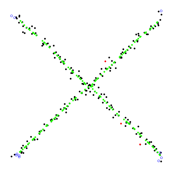
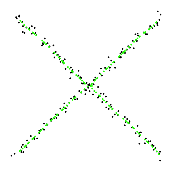
Figure 2.5: X-cross: 200 data points. Black solid dots are data points; Blue circles are the points removed by pre-processing; Red dots are point removed by post-processing; Green dots are the final output of the algorithm.

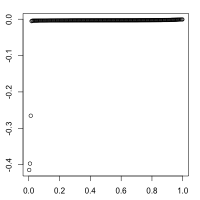
Figure 2.6: Sorted ridgeness values of the output of Algorithm 2 run on the 200 data points with x-cross as ridges without imposing the threshold $\varepsilon_{\eta}$. A clear jump is visible between the ridgeness values close to zero and those of non-global modes. This observation then informed our choice of $\varepsilon_{\eta}=-0.1$. The points below this threshold correspond to the red dots in the left panel of Figure 2.5.

Our algorithms are also implemented using two additional data sets, as shown Figures 2.7 and 2.8, for which we only present the final results after the pre-processing and post-processing steps, with the black and green dots having the same meaning as in Figure 2.5.

Figure 2.7: Circle: 200 data points.

Figure 2.8: Spiral: 200 data points.

2.6.3 Other more practical aspects

In Algorithm 1, we need to compute $\nabla\widehat{\xi}(x)$ and eigenvalues and eigenvectors of $\nabla^{2}\widehat{\eta}(x).$ In the following we present the formulas for them. Let vec be the matrix vectorization operator such that $\text{vec}(A)$ stacks all the columns of a matrix $A$ into a vector.

As for $\nabla\widehat{\xi}(x)$, we have the following by using the product rule for matrix calculus:

$$\nabla\widehat{\xi}(x) =(\nabla\widehat{f}(x)^{\top}\otimes\mathbf{I}_{d})\nabla[\widehat{V}_{\perp}(x)\widehat{V}_{\perp}(x)^{\top}]+\widehat{V}_{\perp}(x)\widehat{V}_{\perp}(x)^{\top}\nabla^{2}\widehat{f}(x)$$

$$=(\nabla\widehat{f}(x)^{\top}\otimes\mathbf{I}_{d})\nabla[\widehat{V}_{\perp}(x)\widehat{V}_{\perp}(x)^{\top}]+\widehat{V}_{\perp}(x)\widehat{\Lambda}_{\perp}(x)\widehat{V}_{\perp}(x)^{\top},$$ (2.15)

where $\widehat{\Lambda}_{\perp}=\text{diag}(\widehat{\lambda}_{r+1},\cdots,\widehat{\lambda}_{d})$, $\nabla[\widehat{V}_{\perp}(x)\widehat{V}_{\perp}(x)^{\top}]=\frac{d\text{ vec}[\widehat{V}_{\perp}(x)\widehat{V}_{\perp}(x)^{\top}]}{dx^{\top}}\in\mathbb{R}^{d^{2}\times d}$, and $\otimes$ denotes Kronecker product.

The Hessian $\nabla^{2}\widehat{\eta}(x)$ is given by

$$\nabla^{2}\widehat{\eta}(x)=-(\mathbf{I}_{d}\otimes\widehat{\xi}(x)^{\top})\nabla(\nabla\widehat{\xi}(x))-\nabla\widehat{\xi}(x)^{\top}\nabla\widehat{\xi}(x),$$ (2.16)

where $\nabla(\nabla\widehat{\xi}(x))$ can be found by using the product rule:

$$\nabla(\nabla\widehat{\xi}(x))= [(\nabla[\widehat{V}_{\perp}(x)\widehat{V}_{\perp}(x)^{\top}])^{\top}\otimes\mathbf{I}_{d}]\nabla(\nabla\widehat{f}(x)^{\top}\otimes\mathbf{I}_{d})$$

$$+(\mathbf{I}_{d}\otimes(\nabla\widehat{f}(x)^{\top}\otimes\mathbf{I}_{d}))\nabla(\nabla[\widehat{V}_{\perp}(x)\widehat{V}_{\perp}(x)^{\top}])$$

$$+(\nabla^{2}\widehat{f}(x)\otimes\mathbf{I}_{d})\nabla[\widehat{V}_{\perp}(x)\widehat{V}_{\perp}(x)^{\top}]$$

$$+(\mathbf{I}_{d}\otimes[\widehat{V}_{\perp}(x)\widehat{V}_{\perp}(x)^{\top}])\nabla(\nabla^{2}\widehat{f}(x)).$$

Here $\nabla(\nabla\widehat{f}(x)^{\top}\otimes\mathbf{I}_{d})=(\mathbf{I}_{d}\otimes\text{vec}(\mathbf{I}_{d}))\nabla^{2}\widehat{f}(x)$. Furthermore, we can find the expressions of $\nabla[\widehat{V}_{\perp}(x)\widehat{V}_{\perp}(x)^{\top}]$ and $\nabla(\nabla[\widehat{V}_{\perp}(x)\widehat{V}_{\perp}(x)^{\top}])$, which by the chain rule involves the third and fourth derivatives of $\widehat{f}$, respectively. For example, for $\ell=1,\cdots,d$, the $\ell$th column of $\nabla[\widehat{V}_{\perp}(x)\widehat{V}_{\perp}(x)^{\top}]$ is given by the vectorization of

$$\sum_{i=1}^{k}\sum_{j=k+1}^{d}\frac{1}{\widehat{\lambda}_{j}(x)-\widehat{\lambda}_{i}(x)}[\widehat{V}_{j}(x)\widehat{V}_{j}(x)^{\top}\widehat{H}_{\ell}(x)\widehat{V}_{i}(x)\widehat{V}_{i}(x)^{\top}+\widehat{V}_{i}(x)\widehat{V}_{i}(x)^{\top}\widehat{H}_{\ell}(x)\widehat{V}_{j}(x)\widehat{V}_{j}(x)^{\top}],$$ (2.17)

where $\widehat{H}_{\ell}(x)$ is the partial derivative of $\nabla^{2}\widehat{f}(x)$ with respective to the $\ell$th component of $x$. See Qiao (2020) for some relevant calculations.

Algorithm 2 avoids direct computation of these third and fourth derivatives of $\widehat{f}$, and thus has some computational advantages in practice. Indeed the connection between the two algorithms can be understood in such a way that the symbolic computation of $\nabla\widehat{\eta}$ and $\nabla^{2}\widehat{\eta}$ in Algorithm 1 are replaced by their numerical approximations ($\nabla\widehat{\eta}_{\tau}$ and $\nabla^{2}\widehat{\eta}_{\tau}$) based on the evaluations of $\widehat{\eta}$ in Algorithm 2. In practice, we implement the computation of $\nabla\widehat{\eta}_{\tau}$ and $\nabla^{2}\widehat{\eta}_{\tau}$ as follows. Let $\{x_{i},i=1,2,\cdots\}$ be a grid over $\mathbb{R}^{d}$ with grid length $\rho<\tau$. Then $\nabla\widehat{\eta}_{\tau}$ is approximated by

$$\frac{\rho^{d}}{\tau^{d}}\sum_{i}\nabla\Big{[}L\left(\frac{x-x_{i}}{\tau}\right)\Big{]}\widehat{\eta}(x_{i}),$$

and $\nabla^{2}\widehat{\eta}_{\tau}$ can be approximated in a similar way. The kernel $L$ is often chosen with bounded support or as the Gaussian kernel with truncation so that there are only a limited number of grid points involved in the above summation.

2.7 Other variants

Here we briefly discuss two other variants of our algorithm.

The first variant is a SCMS type algorithm. The original mean shift algorithm proposed by Fukunaga and Hostetler (1975) is a gradient ascent algorithm using the logarithm transformation of kernel density estimates, which is analyzed in Arias-Castro et al. (2016). More specifically, for any $x_{0}\in\mathbb{R^{d}}$, they consider the sequence $x_{j+1}=x_{j}+a\nabla\log\widehat{f}(x_{j})$, $j=0,1,2,\cdots,$ whose limit is a local mode of $\widehat{f},$ provided some regularity assumptions hold.

A similar idea can be applied to our algorithms as well. Let $g:\mathbb{R}_{\leq 0}\rightarrow\mathbb{R}_{>0}$ be a (known) twice differentiable increasing positive function. In Algorithm 1, we can replace the derivatives (and the induced eigenvalues and eigenvectors) of $\widehat{\eta}$ by those of $\log(g(\widehat{\eta}))$. Note that $\widehat{\eta}$ by definition is non-positive and this explains the need for a positive transformation function $g$. More specifically, let $\widehat{V}^{*}_{g,\perp}(x)$ be a $d\times(d-k)$ matrix whose columns consist of the orthonormal eigenvectors of the Hessian of $\log(g(\widehat{\eta}))$ corresponding to its smallest $(d-k)$ eigenvalues. Let $\widehat{\xi}_{g}^{*}(x)=\widehat{V}^{*}_{g,\perp}(x)\big{[}\widehat{V}^{*}_{g,\perp}(x)\big{]}^{\top}\nabla\log(g(\widehat{\eta}(x))).$ Then the update step (2.13) in Algorithm 1 can be replaced by

$$y_{i}^{j+1}=y_{i}^{j}+a\widehat{\xi}_{g}^{*}(y_{i}^{j}),$$

which is a SCMS type algorithm. Algorithm 2 can be modified in a similar way.

The second variant is based on modified objective functions in the optimization. For some $q>0$, and assuming that $\widehat{f}(x)>0$, write

$$\widehat{s}_{q}(x)=\frac{\widehat{\eta}(x)}{[\widehat{f}(x)]^{q}}.$$ (2.18)

We have that $\widehat{s}_{q}\leq 0$ and $\widehat{s}_{q}=0$ on $\text{Ridge}(\widehat{f}\,)$, and finding minimizers of $\widehat{s}_{q}$ and $\widehat{\eta}$ is equivalent. Thus we can replace the derivatives (and the induced eigenvalues and eigenvectors) of $\widehat{\eta}$ by those of $\widehat{s}_{q}$. Recall that our basic algorithms can possibly return non-global modes of the ridgeness function depending on the start points, and thus requires a pruning process (see subsection 2.6). The numerator in (2.18) is a penalization for low density. The heuristic underlying the introduction of this penalization is to sharpen the ridgeness function near the ridge, so as to potentially accelerate the algorithm and enlarge the set of starting points whose corresponding limit points are global maxima.

The theoretical analyses of these two variants are not explicitly given in this paper, although they are straightforward extensions by following the same procedure as presented for Algorithms 1 and 2 below.

2.8 Notation, assumptions and some technical implications

Recall that $\widehat{\xi}^{*}(x)$ and $\widehat{\xi}^{*}_{\tau}(x)$ denotes the projections of the gradients of $\widehat{\eta}(x)$ and $\widehat{\eta}_{\tau}(x)$, respectively, onto the subspace spanned by the trailing $(d-k)$ eigenvectors of $\nabla^{2}\widehat{\eta}$ and $\nabla^{2}\widehat{\eta}_{\tau}$, respectively. Similarly, we define

$$\xi(x)= \;V_{\perp}(x)V_{\perp}(x)^{\top}\nabla f(x),$$

$$\xi^{*}(x)= \;V^{*}_{\perp}(x)\big{[}V^{*}_{\perp}(x)\big{]}^{\top}\nabla\eta(x),$$

where $V_{\bot}=[V_{k+1},\cdots,V_{d}]$ and $V_{\bot}^{*}=[V^{*}_{k+1},\cdots,V^{*}_{d}]$ denote the $d\times(d-k)$ matrices formed by the trailing $(d-k)$ orthonormal eigenvectors of $\nabla^{2}f(x)$ and $\nabla^{2}\eta(x),$ respectively. The eigenvalues of the Hessians $\nabla^{2}f(x)$ and $\nabla^{2}\eta(x)$ are denoted by $\lambda_{1}\geq\cdots\geq\lambda_{d}$ and $\lambda^{*}_{1}\geq\cdots\geq\lambda^{*}_{d},$ respectively. For $\alpha=(\alpha_{1},\cdots,\alpha_{d})^{T}\in\mathbb{N}^{d}$, let $|\alpha|=\alpha_{1}+\cdots+\alpha_{d}$. For a function $g:\mathbb{R}^{d}\rightarrow\mathbb{R}$ with partial derivatives of order $|\alpha|$, define

$$\partial^{(\alpha)}g(x)=\frac{\partial^{|\alpha|}}{\partial^{\alpha_{1}}x_{1}\cdots\partial^{\alpha_{d}}x_{d}}g(x),\;x\in\mathbb{R}^{d}.$$

With slight abuse of notation, we use $\text{Ridge}(g)$ to denote the ridge of any twice differentiable function $g$ restricted to $[0,1]^{d}.$

In the formulations of our theoretical results, we will use the following assumptions. Let $m$ be a positive integer (where our results will require $m\geq 4$).

(A1)_f,m $f>0$ is a density on $\mathbb{R}^{d}$ such that, for some $\epsilon_{0}>0$, $[-\varepsilon_{0},1+\varepsilon_{0}]^{d}$ is contained in the support of $f$; the partial derivatives of $f$ up to order $m$ exist and are bounded and continuous.

For $\delta>0$ and $A\subset\mathbb{R}^{d},$ we define $A^{\delta}=\bigcup_{x\in A}\mathcal{B}(x,\delta),$ where $\mathcal{B}(x,\delta)$ denotes the (open) ball with midpoint $x$ and radius $\delta.$

(A2)_f There exist $\beta,\delta>0$ such that: $|\lambda_{k+1}(x)|>\beta$ for all $x\in\{t\in[0,1]^{d}:\eta(t)=0\}^{\delta}$, and $\lambda_{k}(x)-\lambda_{k+1}(x)<\beta,$ and for all $x\in[0,1]^{d}$. Furthermore, $\text{Ridge}(f)^{\delta}\subset[0,1]^{d}$.

(A3)_f For all $x\in\text{Ridge}(f),$ $\nabla\xi(x)\in\mathbb{R}^{d\times d}$ has rank $d-k.$

(K)_m The kernel function $K:\mathbb{R}^{d}\to[0,\infty)$ is spherically symmetric and integrates to 1. All the partial derivatives up to order $m$ exist and are continuous and bounded. Moreover, for any $\alpha\in\mathbb{N}^{d}$ with $|\alpha|\leq m$, the class of functions

$$\Big{\{}x\mapsto\partial^{(\alpha)}K\Big{(}\frac{x-y}{h}\Big{)}:\,y\in\mathbb{R}^{d},h>0\Big{\}}$$

is a VC-class (see van der Vaart and Wellner, 1996). Also assume $\int_{\mathbb{R}^{d}}K(x)\|x\|^{2}dx<\infty.$

(L) The kernel function $L:\mathbb{R}^{d}\to[0,\infty)$ is spherically symmetric with bounded support and integrates to 1. The partial derivatives of $L$ up to order four exist and are continuous.

Discussion of the assumptions: (i) Assumption (A1)_f,m is made to avoid boundary issues of kernel density estimation on $[0,1]^{d}$. The unit cube can of course be replaced by any compact set in $\mathbb{R}^{d}$. (ii) Assumption (A2)_f is typical in the literature of ridge estimation (see, e.g. Assumption A1 in Genovese et al., 2014). It avoids spurious ridge points under small perturbation. (iii) Assumption (A3)_f implies that $\text{Ridge}(f)$ is a manifold (without boundary). E.g., see Theorem 5.12 in Lee (2013). In particular, this prevents the existence of intersections of the ridge. For ridges with boundary or intersections, our results (except Theorem 16 (iv)) still apply to the part on the ridges strictly bounded away from the boundary and intersections. (v) The VC-class assumption in (K)_m holds if $K$ is of the form $K(x)=\phi(p(x))$ with $\phi:\mathbb{R}\to\mathbb{R}_{\geq 0}$ bounded and of bounded variation, and $p(x)$ a polynomial (see Nolan and Pollard, 1987). In particular this is the case for the Gaussian kernel. (vi) Under the above assumptions, $\eta(x)$ is twice differentiable and the second derivatives are Lipschitz continuous. In particular, the Hessian $\nabla^{2}\eta(x)$ is well-defined, and we have the following properties:

Lemma 2

Under (A1)_f,4, (A2)_f, and (A3)_f, we have $\lambda_{1}^{*}(x)=\cdots=\lambda_{k}^{*}(x)=0$ for all $x\in\text{Ridge}(f)$, and there exist constants $A,\alpha,\delta>0$, such that for all $x\in\text{Ridge}(f)^{\delta},$

$$-\alpha\geq\lambda^{*}_{k+1}(x)\cdots\geq\lambda_{d}^{*}(x)\geq-A.$$ (2.19)

Moreover, the columns of $V^{*}_{\perp}(x)$ span the normal space of $\text{Ridge}(f)$ at $x\in\text{Ridge}(f)$.

Proof  First we show that $\text{Ridge}(f)$ is a compact set. Notice that from assumption (A2)_f,

$$\text{Ridge}(f)=\{x\in[0,1]^{d}:\xi(x)=0,\;\lambda_{k+1}(x)\leq 0\},$$

because the set $\{x\in[0,1]^{d}:\xi(x)=0,\;\lambda_{k+1}(x)=0\}$ is empty. If we treat $V_{\perp}V_{\perp}^{\top}$ as a function of $\nabla^{2}\eta$, due to the assumed positive gap between $\lambda_{k}(x)$ and $\lambda_{k+1}(x)$ in assumption (A2)_f, $V_{\perp}V_{\perp}^{\top}$ is an analytical matrix-valued function on the space of real symmetric matrices by the classical matrix perturbation theory (see Kato, 1995), which further implies that $V_{\perp}V_{\perp}^{\top}$ is a Lipschitz function of $x$ by assumption (A1)_f,4. Since both $\xi(x)$ and $\lambda_{k+1}(x)$ are continuous functions, $\text{Ridge}(f)$ is closed, and hence compact because it is defined on the compact set $[0,1]^{d}.$

We have $\nabla^{2}\eta(x)=-(\mathbf{I}_{d}\otimes\xi(x)^{\top})\nabla(\nabla\xi(x))-\nabla\xi(x)^{\top}\nabla\xi(x)$. Thus, for $x\in\text{Ridge}(f)$, $\nabla^{2}\eta(x)=-\nabla\xi(x)^{\top}\nabla\xi(x),$ which, by using assumption (A3)_f, implies that rank of $\nabla^{2}\eta(x)$ is $d-k$. Hence we have for $x\in\text{Ridge}(f)$,

$$0=\lambda_{1}^{*}(x)=\cdots=\lambda_{k}^{*}(x)>\lambda^{*}_{k+1}(x)\cdots\geq\lambda_{d}^{*}(x).$$

Since $\xi(x)=0$ for all $x\in\text{Ridge}(f)$, under assumption (A1)_f,4, there exists a constant $c_{0}>0$ such that for $\delta^{\prime}>0$ small enough, $\|(\mathbf{I}_{d}\otimes\xi(x)^{\top})\nabla(\nabla\xi(x))\|_{F}\leq c_{0}\delta^{\prime}$ for all $x\in\text{Ridge}(f)^{\delta^{\prime}}$. Also there exists a constant $c_{1}>0$ such that for all $x,y\in\text{Ridge}(f)^{\delta^{\prime}},$ $\|\nabla\xi(x)^{\top}\nabla\xi(x)-\nabla\xi(y)^{\top}\nabla\xi(y)\|_{F}\leq c_{1}\|x-y\|.$ By using Weyl’s inequality (see page 15 of Serre, 2002), we have $|\lambda_{j}^{*}(x)-\lambda_{j}^{*}(y)|\leq 2c_{0}\delta^{\prime}+c_{1}\|x-y\|$, for all $x,y\in\text{Ridge}(f)^{\delta^{\prime}}.$ Therefore (2.19) holds for $\delta>0$ small enough.

Since $\xi(x)=0$ for all $x\in\text{Ridge}(f),$ the row vectors of $\nabla\xi(x)$ span the normal space of $\text{Ridge}(f)$ at $x$, denoted by $\mathcal{N}(x)$. Note that $\mathcal{N}(x)=\{\nabla\xi(x)^{\top}a:\;a\in\mathbb{R}^{d}\}=\{\nabla\xi(x)^{\top}\nabla\xi(x)a:\;a\in\mathbb{R}^{d}\}$, which is the same as the space spanned by the eigenvectors of $\nabla^{2}\eta(x)$ corresponding to the non-zero eigenvalues, i.e., the space spanned by the columns of $V^{*}_{\perp}(x)$.  

2.9 Main results

We will need the following notation:

$$S_{\epsilon}:=\{x\in[0,1]^{d}:\;\eta(x)\geq-\epsilon,\lambda_{k+1}(x)<0\}.$$ (2.20)

Similarly, we define $\widehat{S}_{\epsilon}$ and $\widehat{S}_{\tau,\epsilon}$ by replacing $\eta(x)$ with $\widehat{\eta}(x)$ and $\widehat{\eta}_{\tau}(x),$ respectively, and by also replacing $\lambda_{k+1}(x)$ with $\widehat{\lambda}_{k+1}(x)$.

For any subset $\mathcal{A}\subset\mathbb{R}^{d}$, and $x\in\mathbb{R}^{d}$, let $d(x,\mathcal{A})=\inf_{y\in\mathcal{A}}\|x-y\|$. For another subset $\mathcal{B}\subset\mathbb{R}^{d}$, the Hausdorff distance between $\mathcal{A}$ and $\mathcal{B}$ is defined as

$$d_{H}(\mathcal{A},\mathcal{B})=\max\{\sup_{x\in\mathcal{A}}d(x,\mathcal{B}),\;\sup_{x\in\mathcal{B}}d(x,\mathcal{A})\}.$$

For any $c_{1},c_{2}\in\mathbb{R}$, let $c_{1}\vee c_{2}=\max(c_{1},c_{2})$ and $c_{1}\wedge c_{2}=\min(c_{1},c_{2})$. Finally, we will use $\|A\|_{F}$ to denote Frobenius-norm of a matrix $A$.

Theorem 3

Assume (A1)_f,4, (A2)_f, (A3)_f, (K)₄, $h=o(1),$ and $\frac{\log n}{nh^{d+8}}=o(1)$ as $n\rightarrow\infty$. Then, for any $B>0$ and $n$ large enough, with probability at least $1-n^{-B}$:

$$d_{H}(\text{\rm Ridge}(f),\text{\rm Ridge}(\widehat{f}\,))=O\Big{(}\Big{(}\frac{\log n}{nh^{d+4}}\Big{)}^{1/2}+h^{2}\Big{)}.$$ (2.21)

Proof Using Talagrand’s inequality (see Proposition A.5 in Sriperumbudur and Steinwart, 2012), there exists a constant $C>0$ such that, for all $n\geq 1$, $h\in(0,1)$, $b>1$ and $|\alpha|\leq 4$ with $nh^{d+2|\alpha|}\geq(b\vee|\log h|)$, we have

$$\mathbb{P}\Big{(}\sup_{x\in[0,1]^{d}}|\partial^{(\alpha)}\widehat{f}(x)-\mathbb{E}\partial^{(\alpha)}\widehat{f}(x)|<C\sqrt{\frac{b\vee|\log h|}{nh^{d+2|\alpha|}}}\Big{)}\geq 1-e^{-b}.$$ (2.22)

It follows from standard calculation for kernel density estimation (see, e.g., Lemma 2 of Arias-Castro et al., 2016) that for all $|\alpha|\leq 4,$

$$\sup_{x\in[0,1]^{d}}|\partial^{(\alpha)}f(x)-\mathbb{E}\partial^{(\alpha)}\widehat{f}(x)|=O(h^{(4-|\alpha|)\wedge 2}).$$ (2.23)

Then (2.22) and (2.23) imply that for any $B>0$, on a set $A_{n}$ with probability at least $1-n^{-B}$,

$$\sup_{x\in[0,1]^{d}}|\partial^{(\alpha)}f(x)-\mathbb{E}\partial^{(\alpha)}\widehat{f}(x)|=O\Big{(}\Big{(}\frac{\log n}{nh^{d+4}}\Big{)}^{1/2}+h^{(4-|\alpha|)\wedge 2}\Big{)},$$

for all $|\alpha|\leq 4.$ Observe that, since the eigenvalues of a symmetric matrix are Lipschitz continuous functions, we obtain from that $\sup_{x\in[0,1]^{d}}|\widehat{\lambda}_{k+1}(x)-\lambda_{k+1}(x)|=o(1)$ on $A_{n}$ for $n$ large enough. By assumption (A2)_f, this implies that on $A_{n}$ we have for all $\epsilon\geq 0$ small enough, that $\widehat{S}_{\epsilon}=\big{\{}x\in[0,1]^{d}:\,\widehat{\eta}(x)\geq-\epsilon,\lambda_{k+1}(x)<0\big{\}}$ for $n$ large enough. Denote $\rho_{n}=\sup_{x\in[0,1]^{d}}|\sqrt{-\widehat{\eta}(x)}-\sqrt{-\eta(x)}|$. It follows that on $A_{n},$ we have that for $n$ large enough,

$$\text{Ridge}(\widehat{f}\,)=\widehat{S}_{0}\subset\big{\{}x\in[0,1]^{d}:\;\eta(x)\geq-\rho_{n}^{2},\lambda_{k+1}(x)<0\big{\}}=S_{\rho_{n}^{2}}.$$

We then have on $A_{n},$

$$\sup_{x\in\text{Ridge}(\widehat{f})}d(x,\text{Ridge}(f))=O\Big{(}\Big{(}\frac{\log n}{nh^{d+4}}\Big{)}^{1/2}+h^{2}\Big{)},$$ (2.24)

which follows from (3.14) below, by using that $\rho_{n}=O((\frac{\log n}{nh^{d+4}})^{1/2}+h^{2}).$ Indeed, note that

$$\sqrt{2}\rho_{n} \leq\sup_{x\in[0,1]^{d}}\|\widehat{V}_{\perp}(x)\widehat{V}_{\perp}^{\top}(x)\nabla\widehat{f}(x)-V_{\perp}(x)V_{\perp}^{\top}(x)\nabla f(x)\|$$

$$\leq\sup_{x\in[0,1]^{d}}\|[\widehat{V}_{\perp}(x)\widehat{V}_{\perp}^{\top}(x)-V_{\perp}(x)V_{\perp}^{\top}(x)]\nabla f(x)\|+\sup_{x\in[0,1]^{d}}\|\widehat{V}_{\perp}(x)\widehat{V}_{\perp}^{\top}(x)[\nabla\widehat{f}(x)-\nabla f(x)]\|$$

$$\leq\sup_{x\in[0,1]^{d}}\|\widehat{V}_{\perp}(x)\widehat{V}_{\perp}^{\top}(x)-V_{\perp}(x)V_{\perp}^{\top}(x)\|_{F}\|\nabla f(x)\|+\sup_{x\in[0,1]^{d}}\|\nabla\widehat{f}(x)-\nabla f(x)\|$$

$$\leq\frac{2\sqrt{2}}{\beta}\sup_{x\in[0,1]^{d}}\|\nabla^{2}\widehat{f}(x)-\nabla^{2}f(x)\|_{F}\sup_{x\in[0,1]^{d}}\|\nabla f(x)\|+\sup_{x\in[0,1]^{d}}\|\nabla\widehat{f}(x)-\nabla f(x)\|,$$

where the last step follows from the Davis-Kahan theorem (see Yu et al., 2015). Using (2.22) and (2.23) gives the asserted rate in (2.24). The result in Theorem 5(i) allows us to swap the roles of $f$ and $\widehat{f}$ in (2.24) and get on $A_{n},$

$$\sup_{x\in\text{Ridge}(f)}d(x,\text{Ridge}(\widehat{f}\,))=O\Big{(}\Big{(}\frac{\log n}{nh^{d+4}}\Big{)}^{1/2}+h^{2}\Big{)}.$$ (2.25)

We conclude the proof by combining (2.24) and (2.25).  

Remark 4

Genovese et al. (2014) also gives the same rate of convergence for ridge estimation using the Hausdorff distance. However, their assumptions and methods of proof are different from ours. In particular, in their assumption (A2) they require that $\|[I_{d}-V_{\perp}(x)V_{\perp}(x)^{\top}]\nabla f(x)\|f_{\max,3}(x)\leq\frac{\beta^{2}}{2d^{3}}$ for all $x\in\text{Ridge}(f)^{\delta}$, where $f_{\max,3}(x)$ is the maximum of the absolute values of all the third partial derivatives of $f$ at $x$, and $\beta$ is essentially the same one as given in our (A2)_f. Instead of this assumption, we use (A3)_f, which is weaker (see Lemma 2 in Chen et al., 2015).

2.9.1 Continuous versions of the algorithms

Further notation. Let $U:\mathbb{R}^{d}\rightarrow\mathbb{R}^{d}$ be a vector field, and $x_{0}\in\mathbb{R}^{d}.$ Consider the general autonomous system of ODEs

$$\frac{dx(t)}{dt}=U(x(t)),\;t\in\mathbb{R},$$

where $x:\mathbb{R}\rightarrow\mathbb{R}^{d}$ with $x(0)=x_{0}$. This generates a flow $\pi:\mathbb{R}^{d}\times\mathbb{R}\rightarrow\mathbb{R}^{d}$ such that $\pi(x,0)=x$, $\pi(\pi(x,t),s)=\pi(x,t+s)$ and $\frac{\partial}{\partial t}\pi(x,t)=U(\pi(x,t))$, for $s,t\in\mathbb{R}$. A trajectory, or an integral curve, with a starting point $x_{0}\in\mathbb{R}^{d}$ is denoted by $\pi(x_{0},t)$. Let $\gamma^{*}(x,t),\widehat{\gamma}^{*}(x,t)$ and $\widehat{\gamma}^{*}_{\tau}(x,t)$ denote the flows generated by $\xi^{*},\widehat{\xi}^{*}$ and $\widehat{\xi}^{*}_{\tau}$, respectively.

Theorem 5

Assume (A1)_f,4, (A2)_f, (A3)_f, (K)₄, $h=o(1)$ and $\frac{\log n}{nh^{d+8}}=o(1)$ as $n\rightarrow\infty$. Then, for any $B>0$ and $n$ large enough, with probability at least $1-n^{-B}$:

1. $\widehat{f}$ satisfies assumptions (A1)${}_{\widehat{f},4\;}$, (A2)${}_{\widehat{f}}$, and (A3)${}_{\widehat{f}}$;

2. Continuous version of Algorithm 1: there exists $\epsilon_{0}>0$ such that, for all $0\leq\epsilon\leq\epsilon_{0}$,

   • $\text{\rm Ridge}(\widehat{f}\,)=\{\lim_{t\rightarrow\infty}\widehat{\gamma}^{*}(x,t),x\in\partial\widehat{S}_{\epsilon}\}=\text{\rm Ridge}(\widehat{\eta}\,)\cap\widehat{S}_{\epsilon}.$

3. Continuous version of Algorithm 2: under the additional assumptions (A1)_f,6, (K)₆, (L) and $\frac{\log n}{nh^{d+12}}=o(1)$, and for $\epsilon>0$ small enough,

   • $\text{\rm Ridge}(\widehat{\eta}_{\tau})\cap\widehat{S}_{\tau,\epsilon}=\{\lim_{t\rightarrow\infty}\widehat{\gamma}^{*}_{\tau}(x,t),x\in\partial\widehat{S}_{\tau,\epsilon}\}$ for $\tau>0$ small enough;

   • $d_{H}(\text{\rm Ridge}(\widehat{\eta}_{\tau})\cap\widehat{S}_{\tau,\epsilon},\text{\rm Ridge}(\widehat{f}\,))=O(\tau^{2})$ as $\tau\rightarrow 0$;

   • $d_{H}(\text{\rm Ridge}(\widehat{\eta}_{\tau})\cap\widehat{S}_{\tau,\epsilon},\text{\rm Ridge}(f))=O((\frac{\log n}{nh^{d+4}})^{1/2}+h^{2}+\tau^{2})$ as $\tau\rightarrow 0$.

Proof  (i) Using (2.22) and (2.23), properties (A1)${}_{\widehat{f},4\;}$ and (A2)${}_{\widehat{f}}$ are consequences of the Lipschitz continuity of the eigenvalues as functions of symmetric matrices. Let $\lambda_{d-k}^{\dagger}(A)$ be the $(d-k)$th largest eigenvalue of a symmetric matrix $A$. To show (A3)${}_{\widehat{f}}$, notice that assumption (A3)_f implies that for $\delta>0$ small enough, there exists a constant $a_{0}>0$ such that

$$\inf_{x\in\text{Ridge}(f)^{\delta}}\lambda_{d-k}^{\dagger}(\nabla\xi(x)^{\top}\nabla\xi(x))\geq a_{0}.$$

Due to the perturbation stability of $\lambda_{d-k}^{\dagger}$, we have $\inf_{x\in\text{Ridge}(f)^{\delta}}\lambda_{d-k}^{\dagger}(\nabla\widehat{\xi}(x)^{\top}\nabla\widehat{\xi}(x))\geq\frac{1}{2}a_{0}$ with probability at least $1-n^{-B}$ when $n$ is large. This then implies the rank of $\nabla\widehat{\xi}(x)$ is at least $d-k.$ Furthermore, using the expression of $\nabla\widehat{\xi}(x)$ in (2.6.3) and the calculation in (2.17), it can be seen that $\widehat{V}_{i}(x)^{\top}\nabla\widehat{\xi}(x)=0$, for all $i=1,\cdots,k$, which implies that the rank of $\nabla\widehat{\xi}(x)$ is at most $d-k$. Hence (A3)${}_{\widehat{f}}$ is satisfied.

(ii). Given (i), this is a consequence of Lemma 10 and Theorem 11.

(iii). Given (i), we have the following: For some $\delta>0$, we have for $|\alpha|=0,1,2,$

$$\sup_{x\in[0,1]^{d}}|\partial^{(\alpha)}\widehat{\eta}(x)-\partial^{(\alpha)}\widehat{\eta}_{\tau}(x)|=O(\tau^{2}).$$ (2.26)

This can be shown by using standard techniques for calculating the rate of the bias in kernel density estimation (see, e.g., proof of Lemma 2 in Arias Castro et al., 2016). For $\tau$ small, we have $\text{Ridge}(\widehat{\eta}_{\tau})=\{\lim_{t\rightarrow\infty}\widehat{\gamma}^{*}_{\tau}(x,t),x\in\partial\widehat{S}_{\tau,\epsilon}\}$, as a result of Theorem 14(iii). This is a). Part b) is a consequence of Theorem 14 (iv). Part c) immediately follows from Theorem 3.  

Remark 6

Without the additional assumptions in part (iii) of the above theorem, we can still show that with probability at least $1-n^{-B}$, $\sup_{x\in[0,1]^{d}}|\partial^{(\alpha)}\widehat{\eta}(x)-\partial^{(\alpha)}\widehat{\eta}_{\tau}(x)|=o(1)$ for all $|\alpha|=0,1,2,$ and therefore $d_{H}(\text{\rm Ridge}(\widehat{\eta}_{\tau})\cap\widehat{S}_{\tau,\epsilon},\text{\rm Ridge}(f))=o(1)$ as $\tau\rightarrow 0$.

2.9.2 Discrete approximation: the Euler method

Here we study discrete versions of the algorithms given above. To this end, recall that $\widehat{\xi}^{*}=\widehat{V}^{*}_{\bot}[\widehat{V}^{*}_{\bot}]^{\top}\nabla\widehat{\eta}.$ For a constant $a>0$, let $\widehat{\gamma}^{*}_{a}(x,\ell)$, $\ell=0,1,\cdots,$ be defined as

$$\widehat{\gamma}^{*}_{a}(x,0)=x\qquad\text{and}\qquad\widehat{\gamma}^{*}_{a}(x,\ell+1)=\widehat{\gamma}^{*}_{a}(x,\ell)+a\,\widehat{\xi}^{*}(\widehat{\gamma}^{*}_{a}(x,\ell)),\quad\ell=1,2,\ldots$$

This is a discrete approximation to $\gamma^{*}(x,t),$ $t\geq 0$ using Euler’s method. Similarly, we define the discrete approximation $\widehat{\gamma}^{*}_{a,\tau}(x,\ell)$ of $\widehat{\gamma}^{*}_{\tau}(x,t)$ by replacing $\widehat{\xi}^{*}$ by $\widehat{\xi}^{*}_{\tau}$ (or, in other words, by replacing $\widehat{\eta}$ by $\widehat{\eta}_{\tau}$). The following result says that these discretized approximations can be used to recover the corresponding ridges.

Theorem 7

Assume (A1)_f,6, (A2)_f, (A3)_f, (K)₆, (L), $h=o(1)$ and $\frac{\log n}{nh^{d+12}}=o(1)$ as $n\rightarrow\infty$. Then, for any $B>0$ and $n$ large enough, with probability at least $1-n^{-B}$:

1. Algorithm 1: With $R_{a}(\widehat{f}\,)=\{\lim_{\ell\rightarrow\infty}\widehat{\gamma}^{*}_{a}(x,\ell),x\in\partial\widehat{S}_{\epsilon}\},$ we have for $\epsilon\geq 0$ small enough

   $$d_{H}(\text{\rm Ridge}(\widehat{f}\,),R_{a}(\widehat{f}\,))=o(1)\quad\text{as }a\rightarrow 0.$$ (2.27)

2. Algorithm 2: With $R_{\tau,a}(\widehat{f}\,)=\{\lim_{\ell\rightarrow\infty}\widehat{\gamma}^{*}_{\tau,a}(x,\ell),x\in\partial\widehat{S}_{\tau,\epsilon}\},$ and $\epsilon\geq 0$ small enough, we have

   $$d_{H}(\text{\rm Ridge}(\widehat{f}\,),R_{\tau,a}(\widehat{f}\,))=o(1)\quad\text{as }a\rightarrow 0\text{ and }\tau\rightarrow 0.$$ (2.28)

Proof  The result in (i) follows from Theorem 5(i) and Theorem 16. The result in (ii) is a consequence of Theorem 5 and Corollary 18.  

Remark 8

By using Theorem 16, one can also obtain rates of convergence in (2.27), and one can show that ${\rm Ridge}(\widehat{f}\,)=R_{a}(\widehat{f}\,)$ and $\text{\rm Ridge}(\widehat{\eta}_{\tau})\cap\widehat{S}_{\tau,\epsilon}=R_{\tau,a}(\widehat{f}\,)$ for $d=1$, with probability at least $1-n^{-B}$ for any $B>0$ and $n$ large enough.

3 The mathematical framework for the ODE-based algorithms of ridge extraction

The SCMS type algorithms discussed above can be considered as numerical approximations of trajectories of Ordinary Differential Equations (ODE). These corresponding ODEs (the mathematical models) for our algorithm are analyzed in the following. For the original mean shift algorithm, such theoretical work can be found in Arias-Castro et al. (2016). For the Subspace Constraint Mean Shift algorithm, see Genovese et al. (2014) and Qiao and Polonik (2016) for the theoretical analysis of the corresponding ODE models.

In the following $f$ denotes a generic positive function on $[0,1]^{d}$. While we apply the below results to densities (e.g. to our kernel density estimates), $f$ does not have to integrate to 1.

3.1 Some useful background knowledge of ODEs

A reference for the following material is Wiggins (2003). As above consider

$$\frac{dx(t)}{dt}=U(x(t)),\;t\in\mathbb{R},$$

where $x:\mathbb{R}\rightarrow\mathbb{R}^{d}$ with $x(0)=x_{0}\in\mathbb{R}^{d},$ and $U:\mathbb{R}^{d}\rightarrow\mathbb{R}^{d}$ is a vector field. Let $\pi:\mathbb{R}^{d}\times\mathbb{R}\rightarrow\mathbb{R}^{d}$ denote the corresponding flow.

A compact set $S\subset\mathbb{R}^{d}$ is called a positively invariant set under the above vector field if for any $x_{0}\in S$ we have $\pi(x_{0},t)\in S$ for all $t\geq 0$. We assume that the boundary of $S$ is a $\mathbf{C}^{1}$ manifold. A point $\bar{x}$ is called an equilibrium point, or fixed point, if $U(\bar{x})=0$. Let $\mathcal{A}\subset S$ be the set of all equilibrium points in $S$. A continuously differentiable scalar-valued function $V$ defined on $S$ is called a Lyapunov function if it satisfies: $\frac{dV(x(t))}{dt}\leq 0$ for all $x(t)\in S$. We also define two set

$$E=\left\{x\in S\,:\;\;\frac{dV(x(t))}{dt}=0\right\},$$ (3.1)

$$M=\bigcup_{x_{0}\in E}\big{\{}\pi(x_{0},t),t>0\,:\;\pi(x_{0},t)\in E\text{ for all }t>0\big{\}}.$$ (3.2)

Note that $\mathcal{A}\subset M\subset E.$ We will use LaSalle’s Invariance Principle (see Theorem 8.3.1, Wiggins, 2003), which states:

Theorem 9

For all $x\in S$, $\pi(x,t)\rightarrow M$ as $t\rightarrow\infty$.

Later LaSalle’s Theorem will be applied with $M=E=\text{Ridge}(f).$

3.2 ODE theory for ridge extraction

Recall that $\eta(x)=-\frac{1}{2}\|V_{\perp}(x)^{\top}\nabla f(x)\|^{2}=-\frac{1}{2}\|\xi(x)\|^{2}$. Also recall the definition of $S_{\epsilon}$ given in (2.20). The following lemma states that in a neighborhood of the ridge of $f$, the ridge of the ridgeness function $\eta$ equals the ridge of $f$.

Lemma 10

Assuming (A1)_f,4, (A2)_f, and (A3)_f, there exists an $\epsilon_{0}>0$ such that

$$\text{\rm Ridge}(f)=\text{\rm Ridge}(\eta)\cap S_{\epsilon}\qquad\forall\;0<\epsilon<\epsilon_{0}.$$

Proof  First we show that $\text{\rm Ridge}(f)\subset\text{\rm Ridge}(\eta)\cap S_{\epsilon}$. We have $\nabla\eta(x)=-\nabla\xi(x)^{\top}\xi(x)$ for $x\in[0,1]^{d}.$ Thus, for $x\in\text{Ridge}(f)$ (meaning that $\xi(x)=0$), we have $\nabla\eta(x)=0,$ and hence $\xi^{*}(x)=0$. Then $\text{\rm Ridge}(f)\subset\text{\rm Ridge}(\eta)\cap S_{\epsilon}$ is a direct consequence of Lemma 2.

Next we show that $\text{Ridge}(\eta)\cap S_{\epsilon}\subset\text{Ridge}(f)$ for $\epsilon$ small enough. To this end we show that

$$\|\xi^{*}(x)\|>0\quad\text{for all }x\in S_{\epsilon}\backslash\text{Ridge}(f),$$ (3.3)

which implies the result. Note that $S_{\epsilon}\subset\text{Ridge}(f)^{\delta}$ when $\epsilon$ is small enough. See (3.14) below. For any $x\in S_{\epsilon}\backslash\text{Ridge}(f)$, let $x_{0}\in\text{Ridge}(f)$ be the projection of $x$ onto $\text{Ridge}(f)$, that is, there exists a $\delta_{x}\in(0,\delta)$, such that we can write $x=x_{0}+\delta_{x}u$, where $u=u(x)\in\mathscr{N}(x_{0})$ is a unit vector with ${\mathscr{N}}(x_{0})$ the normal space to the ridge at $x_{0}$. Notice that by using Lemma 2, ${\mathscr{N}}(x_{0})=\{V^{*}_{\bot}(x_{0})a:\,a\in\mathbb{R}^{d-k}\}$. We will show that there exists an $\epsilon>0$, such that $\|\nabla\eta(x)\|>0$ for all $x\in S_{\epsilon}\setminus{\rm Ridge}(f)$. Using Lipschitz continuity of the fourth partial derivatives of $f$, there exists a constant $\kappa_{1}>0$ such that $\|\nabla^{2}\eta(x_{0})-\nabla^{2}\eta(x_{1})\|_{F}\leq\kappa_{1}\|x_{0}-x_{1}\|$ for all $x_{1}\in\mathcal{B}(x_{0},\delta).$ Then we can write

$$\nabla\eta(x) =\nabla\eta(x_{0})+\nabla^{2}\eta(x_{0})(x-x_{0})+R_{1}(x)$$

$$=\delta_{x}\nabla^{2}\eta(x_{0})u+R_{1}(x),$$ (3.4)

where $\|R_{1}(x)\|\leq\kappa_{1}\delta_{x}^{2}$. Note that $\nabla^{2}\eta(x_{0})=\sum_{j=k+1}^{d}\lambda_{j}^{*}(x_{0})V_{j}^{*}(x_{0})V_{j}^{*}(x_{0})^{\top}$ by Lemma 2 and $u$ is a unit vector in the space spanned by $V_{k+1}^{*}(x_{0}),\cdots,V_{d}^{*}(x_{0})$. Hence $A\geq|\lambda_{d}^{*}(x_{0})|\geq\|\nabla^{2}\eta(x_{0})u\|\geq|\lambda_{k+1}^{*}(x_{0})|\geq\alpha$, where $\alpha$ and $A$ are positive constants given in Lemma 2. Thus, for $\epsilon>0$ small enough (and hence $\delta_{x}$ is small), we have $\|\nabla\eta(x)\|>0$.

Next we show that $\frac{|\langle\nabla\eta(x),u(x)\rangle|}{\|\nabla\eta(x)\|}$ is bounded from below. Using (3.2) we have that $|\langle\nabla\eta(x),u(x)\rangle|\geq\delta_{x}|\lambda_{k+1}^{*}(x_{0})|-\kappa_{1}\delta_{x}^{2},$ and

$$\frac{|\langle\nabla\eta(x),u(x)\rangle|}{\|\nabla\eta(x)\|}\geq\frac{\delta_{x}|\lambda_{k+1}^{*}(x_{0})|-\kappa_{1}\delta_{x}^{2}}{\delta_{x}|\lambda_{d}^{*}(x_{0})|+\kappa_{1}\delta_{x}^{2}}.$$

For $\epsilon$ (and hence $\delta_{x}$) small enough, the right-hand side is bounded by a positive constant from below, say,

$$\frac{|\langle\nabla\eta(x),u(x)\rangle|}{\|\nabla\eta(x)\|}\geq\frac{1}{2}\frac{|\lambda_{k+1}^{*}(x_{0})|}{|\lambda_{d}^{*}(x_{0})|}.$$

Since $u$ can be written as $V_{\perp}^{*}(x_{0})a$ with $a\in\mathbb{R}^{d-k}$ and $\|a\|=1$, we have by using the Cauchy-Schwarz inequality that $|\langle\nabla\eta(x),u(x)\rangle|=|\nabla\eta(x)^{\top}V_{\perp}^{*}(x_{0})a|\leq\|V_{\perp}^{*}(x_{0})^{\top}\nabla\eta(x)\|=\|V_{\perp}^{*}(x_{0})V_{\perp}^{*}(x_{0})^{\top}\nabla\eta(x)\|,$ and thus

$$\frac{\|V_{\perp}^{*}(x_{0})V_{\perp}^{*}(x_{0})^{\top}\nabla\eta(x)\|}{\|\nabla\eta(x)\|}\geq\frac{1}{2}\frac{|\lambda_{k+1}^{*}(x_{0})|}{|\lambda_{d}^{*}(x_{0})|}.$$ (3.5)

On the other hand, the angle between the eigenspace spanned by $V_{\perp}^{*}(x_{0})$ and $V_{\perp}^{*}(x)$ should be small if $\delta_{x}$ is small because $\nabla^{2}\eta$ is a continuous function of $x$. This can be seen by using the Davis-Kahan inequality:

$$\|V_{\perp}^{*}(x_{0})V_{\perp}^{*}(x_{0})^{\top}-V_{\perp}^{*}(x)V_{\perp}^{*}(x)^{\top}\|_{F}\leq\frac{2\sqrt{2}\|\nabla^{2}\eta(x_{0})-\nabla^{2}\eta(x)\|_{F}}{|\lambda_{k+1}^{*}(x_{0})|}\leq\frac{2\sqrt{2}\kappa_{1}\delta_{x}}{|\lambda_{k+1}^{*}(x_{0})|}.$$ (3.6)

Hence using (3.5) and (3.6),

$$\frac{\|\xi^{*}(x)\|}{\|\nabla\eta(x)\|}=\frac{\|V_{\perp}^{*}(x)V_{\perp}^{*}(x)^{\top}\nabla\eta(x)\|}{\|\nabla\eta(x)\|}\geq\frac{1}{2}\frac{|\lambda_{k+1}^{*}(x_{0})|}{|\lambda_{d}^{*}(x_{0})|}-\frac{2\sqrt{2}\kappa_{1}\delta_{x}}{|\lambda_{k+1}^{*}(x_{0})|},$$

which can be bounded from below by a positive constant when $\epsilon$ (and hence $\delta_{x}$) is small enough. This is (3.3).  

Recall that $\frac{\partial\gamma^{*}(x,t)}{\partial t}=\xi^{*}(\gamma^{*}(x,t)),t\in\mathbb{R}$, which is the mathematical model of Algorithm 1. There exists a positive $\epsilon>0$ such that $S_{\epsilon}$ is a positively invariant set corresponding to this flow. This can be seen as follows. Consider the derivative of $\eta(\gamma^{*}(x,t))$ with respect to $t$:

$$\frac{\partial\eta(\gamma^{*}(x,t))}{\partial t}=[\nabla\eta(\gamma^{*}(x,t))]^{\top}V_{\perp}^{*}(\gamma^{*}(x,t))[V_{\perp}^{*}(\gamma^{*}(x,t))]^{\top}\nabla\eta(\gamma^{*}(x,t))=\|\xi^{*}(\gamma^{*}(x,t))\|^{2}\geq 0.$$ (3.7)

In other words, $\eta$ is always non-decreasing along the trajectories of the flow. Indeed, notice that for $\epsilon>0$ small enough, $\|\xi^{*}(\gamma^{*}(x,t))\|>0$ for all $x\in S_{\epsilon}\backslash$Ridge($f$) (or when $t<\infty$) based on Lemma 10. In other words, $\xi^{*}$ is a gradient-like vector field with respect to $\eta$ (see page 45, Nicolaescu, 2011), and it follows that $S_{\epsilon}$ is a positively invariant set as we have claimed. Note that Ridge($f$) is the set of all the equilibrium points in $S_{\epsilon}$. A natural choice for a Lyapunov function $V$ is

$$V(x)=-\eta(x).$$

Since $\frac{\partial V(\gamma^{*}(x,t))}{\partial t}=-\langle\nabla\eta(\gamma^{*}(x,t)),\xi^{*}(\gamma^{*}(x,t))\rangle=-\|\xi^{*}(\gamma^{*}(x,t))\|^{2}\leq 0$, this indeed is a Lyapunov function. Notice further that this derivative is equal to zero only when $x\in$ Ridge($f$). Therefore, for the sets $E$ and $M$ given in (3.1) and (3.2), we have $E=M=$ Ridge($f$).

Theorem 11

Assume that (A1)_f,4, (A2)_f, and (A3)_f hold. There exists $\epsilon>0$ such that:

1. For each $x\in S_{\epsilon}\backslash$Ridge($f$), there is a unique path $\gamma^{*}$ passing through $x$.

2. For each $x\in S_{\epsilon}$ as a starting point, the path $\gamma^{*}(x,t)$ converges to a point on Ridge($f$), as $t\rightarrow+\infty$.

3. $\text{Ridge}(f)=\{\lim_{t\rightarrow\infty}\gamma^{*}(x,t):x\in\partial S_{\epsilon}\},$ where $\partial S_{\epsilon}$ is the boundary of $S_{\epsilon}$.

Proof  (i) is very similar to Lemma 2 in Genovese et al. (2014) and the proof is similar, too. Details are omitted. (ii) follows from the above discussion by an application of LaSalle’s Invariance Principle. Next we prove (iii), for which we will use the technique in the proof of Theorem 2.6 in Nicolaescu (2011). Recall that the vector field generated by $\xi^{*}$ is gradient-like. Let

$$\zeta:=\frac{\xi^{*}}{\|\xi^{*}\|^{2}},$$ (3.8)

and let $\gamma^{\dagger}$ by the integral curve generated by this rescaled vector field, that is,

$$\frac{\partial\gamma^{\dagger}(x,t)}{\partial t}=\zeta(\gamma^{\dagger}(x,t)),\quad\gamma^{\dagger}(x,0)=x.$$ (3.9)

We first show (iii) with $\gamma^{*}$ replaced by $\gamma^{\dagger}.$ Observe that (see (3.7))

$$\frac{\partial\eta(\gamma^{\dagger}(x,t))}{\partial t}=1.$$ (3.10)

In other words, the level of $\eta$ can be used to parametrize the integral curves $\gamma^{\dagger}(x,t)$, so that for any $\epsilon_{1},\epsilon_{2}\in(0,\epsilon)$ with $\epsilon_{1}>\epsilon_{2}$, we have

$$\partial S_{\epsilon_{1}}=\{\gamma^{\dagger}(x,\epsilon_{2}-\epsilon_{1}):x\in\partial S_{\epsilon_{2}}\},$$ (3.11)

$$\partial S_{\epsilon_{2}}=\{\gamma^{\dagger}(x,\epsilon_{1}-\epsilon_{2}):x\in\partial S_{\epsilon_{1}}\}.$$ (3.12)

Both (3.11) and (3.12) are similar to Theorem 2.6 in Nicolaescu (2011). We only show (3.11). Using (3.10), it is clear that for any $x\in{\partial}S_{\epsilon_{2}}$, $\gamma^{\dagger}(x,\epsilon_{2}-\epsilon_{1})\in\partial S_{\epsilon_{1}}$. This means $\{\gamma^{\dagger}(x,\epsilon_{2}-\epsilon_{1}):x\in\partial S_{\epsilon_{2}}\}\subset\partial S_{\epsilon_{1}}$. Now define $\widetilde{\gamma}^{\dagger}$ as the solution of

$$\frac{\partial\widetilde{\gamma}^{\dagger}(x,t)}{\partial t}=-\zeta(\widetilde{\gamma}^{\dagger}(x,t)),\qquad\widetilde{\gamma}^{\dagger}(x,0)=x.$$ (3.13)

Then, similar to (3.10), we have $\frac{\partial\eta(\widetilde{\gamma}^{\dagger}(x,t))}{\partial t}=-1.$ Therefore for any $x\in\partial S_{\epsilon_{1}}$, there exists $\widetilde{x}=\widetilde{\gamma}^{\dagger}(x,\epsilon_{2}-\epsilon_{1})$ so that $x=\gamma^{\dagger}(\widetilde{x},\epsilon_{2}-\epsilon_{1})$. This means that $\partial S_{\epsilon_{1}}\subset\{\gamma^{\dagger}(x,\epsilon_{2}-\epsilon_{1}):x\in\partial S_{\epsilon_{2}}\}$. Hence (3.11) is verified.

Furthermore, as will be shown below, one can find constants $L_{1},L_{2}>0$ such that for all $\epsilon^{\prime}\geq 0$ small enough

$$L_{1}\sqrt{\epsilon^{\prime}}\leq d_{H}(\partial S_{\epsilon^{\prime}},\text{Ridge}(f))=d_{H}(\partial S_{\epsilon^{\prime}},S_{0})\leq L_{2}\sqrt{\epsilon^{\prime}},$$ (3.14)

where $d_{H}$ is the Hausdorff distance. By using (3.11) and (3.12), this means that, for all $\epsilon^{\prime}>0$ small enough

$$L_{1}\sqrt{\epsilon^{\prime}}\leq d_{H}(\{\gamma^{\dagger}(x,{\epsilon-\epsilon^{\prime}}):x\in{\partial}S_{\epsilon}\},\text{Ridge}(f))\leq L_{2}\sqrt{\epsilon^{\prime}}.$$ (3.15)

Next we show that

$$\text{Ridge}(f)=\{\lim_{t\rightarrow\epsilon}\gamma^{\dagger}(x,t):x\in\partial S_{\epsilon}\}.$$ (3.16)

Recall that $\text{Ridge}(f)$ is a compact set (see proof of Lemma 2). The set $\{\lim_{t\rightarrow\epsilon}\gamma^{\dagger}(x,t):x\in\partial S_{\epsilon}\}$ is also compact. This is because $\lim_{t\rightarrow\epsilon}\gamma^{\dagger}(x,t)$ is a continuous function of $x$ (see Fact 6 below) and $\partial S_{\epsilon}$ is a compact set. Suppose that $\text{Ridge}(f)\neq\{\lim_{t\rightarrow\epsilon}\gamma^{\dagger}(x,t):x\in\partial S_{\epsilon}\}.$ Then there must exist a constant $\delta_{0}>0$ such that $\delta_{0}\leq d_{H}(\{\lim_{t\rightarrow\epsilon}\gamma^{\dagger}(x,t):x\in\partial S_{\epsilon}\},\text{Ridge}(f))$, which further implies that there exists $x_{0}\in\partial S_{\epsilon}$ and $\epsilon_{0}>0$ such that for all $0<\epsilon^{\prime}\leq\epsilon_{0}$ we have $d_{H}(\gamma^{\dagger}(x,\epsilon-\epsilon^{\prime}),\text{Ridge}(f))\geq\delta_{0}$. This contradicts (3.15) and therefore (3.16) has to be true.

Next we show that $\gamma^{\dagger}(x,\cdot)$ and $\gamma^{*}(x,\cdot)$ have the same trajectories, which shows (iii). To this end we show a reparameterization relation between the two flows. For each $x\in\partial S_{\epsilon},$ let

$$s(t)= \int_{0}^{t}\|\xi^{*}(x,u)\|^{2}du$$

$$= \int_{0}^{t}\left[\frac{\partial\eta(\gamma^{*}(x,u))}{\partial u}\right]du$$

$$= \eta(\gamma^{*}(x,t))-\eta(\gamma^{*}(x,0))$$

$$= \eta(\gamma^{*}(x,t))-\eta(x).$$

Note that we have suppressed the dependence of $s(t)$ on $x$ in the notation. Let $t(s)$ be the inverse of $s(t)$. Then $t(0)=0,$ and

$$\frac{dt(s)}{ds}=\frac{1}{\|\xi^{*}(x,s)\|^{2}}.$$ (3.17)

We obtain $\gamma^{\dagger}(x,s)=\gamma^{*}(x,t(s))$, because

$$\frac{\partial\gamma^{*}(x,t(s))}{\partial s}=\zeta(\gamma^{\dagger}(x,s)),\;\gamma^{*}(x,t(0))=x.$$ (3.18)

Note that as $t\rightarrow\infty$, we have $s(t)\rightarrow\eta(\gamma^{*}(x,\infty))-\eta(x)=\epsilon$ for all $x\in S_{\epsilon}$, because $\gamma^{*}(x,\infty)\in$ Ridge($f$). Hence $\lim_{t\rightarrow\infty}\gamma^{*}(x,t)=\lim_{s\rightarrow\epsilon}\gamma^{\dagger}(x,s)$ for all $x\in S_{\epsilon}$.

It remains to prove (3.14). For any $b\in\mathbb{R}^{d}$, consider

$$M_{b}:=\{x\in[0,1]^{d}:\;\xi(x)=b,\lambda_{k+1}(x)<0\},$$

and note that $S_{\epsilon^{\prime}}=\bigcup_{\{b:\frac{1}{2}\|b\|^{2}\leq\epsilon^{\prime}\}}M_{b}$ for all $\epsilon^{\prime}\geq 0$. We will show that for all $\|b\|$ small enough, $C_{1}\|b\|\leq d_{H}(M_{b},\text{Ridge}(f))\leq C_{2}\|b\|$ for some positive constants $C_{1},C_{2}$. For any $x\in M_{b}$, let $x_{0}$ be its projection point on $\text{Ridge}(f)$. There exists a unit vector $u=u(x)\in\mathscr{N}(x_{0})$ and $\delta_{x}>0$ such that $x=x_{0}+\delta_{x}u$. Using a Taylor expansion, we get

$$\xi(x)=\xi(x_{0})+\nabla\xi(x_{0})(x-x_{0})+R_{1}(x)=\delta_{x}\nabla\xi(x_{0})u+R_{2}(x),$$

where $\|R_{2}(x)\|\leq\kappa_{2}\delta_{x}^{2},$ for a constant $\kappa_{2}>0$ for all $x\in M_{b}$. Therefore

$$\|b\|^{2}=\|\xi(x)\|^{2}=\delta_{x}^{2}u^{\top}\nabla\xi(x_{0})^{\top}\nabla\xi(x_{0})u+R_{3}(x),$$

where $|R_{3}(x)|\leq\kappa_{3}\delta_{x}^{3},$ for a constant $\kappa_{3}>0$ for all $x\in M_{b}$. Let $\omega_{\max}(x)$ and $\omega_{\min}(x)$ be the largest and the $(d-k)$th largest eigenvalues of $\nabla\xi(x)^{\top}\nabla\xi(x)$, respectively. For $x_{0}\in\text{Ridge}(f)$, we have $\omega_{\min}(x_{0})=-\lambda_{k+1}^{*}(x_{0})$ and $\omega_{\max}(x_{0})=-\lambda_{d}^{*}(x_{0})$ because $\nabla^{2}\eta(x_{0})=-\nabla\xi(x_{0})^{\top}\nabla\xi(x_{0}).$ Observe that the first $k$ eigenvalues $\lambda^{*}_{i}(x_{0}),i=1,\ldots,k$ of $\nabla\xi(x_{0})^{\top}\nabla\xi(x_{0})$ are zero, and that $\lambda_{i}^{*}(x_{0})<0$, $i=k+1,\cdots,d.$ Moreover, $u$ is in the space spanned by $V_{k+1}^{*}(x_{0}),\cdots,V_{d}^{*}(x_{0})$. So when $\|b\|$ is small (and hence $\delta_{x}$ is small), we have that,

$$2|\lambda_{d}^{*}(x_{0})|\delta_{x}^{2}\geq 2\omega_{\max}(x_{0})\delta_{x}^{2}\geq\|b\|^{2}\geq\frac{\omega_{\min}(x_{0})}{2}\delta_{x}^{2}=\frac{|\lambda_{k+1}^{*}(x_{0})|}{2}\delta_{x}^{2}.$$ (3.19)

Since $\delta_{x}=d(x,\text{Ridge}(f))=\inf_{y\in\text{Ridge}(f)}\|x-y\|$, we have for all $b\in\mathbb{R}^{d}$ such that $\frac{1}{2}\|b\|^{2}=\epsilon^{\prime}$ is small enough,

$$\sup_{x\in M_{b}}d(x,\text{Ridge}(f))\leq\sqrt{\frac{2}{|\lambda_{k+1}^{*}(x_{0})|}}\|b\|\leq\sqrt{\frac{2}{|\lambda_{k+1}^{*}(x_{0})|}}\,\sqrt{2\epsilon^{\prime}}\leq\sqrt{\frac{4}{\alpha}}\sqrt{\epsilon^{\prime}},$$ (3.20)

$$\sup_{x\in M_{b}}d(x,\text{Ridge}(f))\geq\sqrt{\frac{1}{2|\lambda_{d}^{*}(x_{0})|}}\|b\|\geq\sqrt{\frac{1}{2|\lambda_{d}^{*}(x_{0})|}}\,\sqrt{2\epsilon^{\prime}}\geq\sqrt{\frac{1}{A}}\sqrt{\epsilon^{\prime}},$$ (3.21)

where $A\geq\alpha>0$ are given in Lemma 2.

The other direction can be proved in a similar way, as given as follows. Now let $x$ be a point on $\text{Ridge}(f)$, and $x_{0}$ be its projection on $M_{b}$, such that $x=x_{0}+\delta_{x}u$, where $\delta_{x}=\|x-x_{0}\|>0$, and $u\in\mathscr{N}(x_{0})$ is a unit normal vector of $M_{b}$ at $x_{0}$. Following the above analysis (in particular (3.19)), when $\|b\|$ is small enough, we still have $2\omega_{\max}(x_{0})\delta_{x}^{2}\geq\|b\|\geq\frac{1}{2}\omega_{\min}(x_{0})\delta_{x}^{2}$. Since $\omega$ is a continuous function in a neighborhood of $\text{Ridge}(f)$, we have that $4A\delta_{x}^{2}\geq\|b\|^{2}\geq\frac{1}{4}\alpha\delta_{x}^{2}$ for all $\|b\|$ small enough. Therefore for all $b\in\mathbb{R}^{d}$ such that $\frac{1}{2}\|b\|^{2}=\epsilon^{\prime}$ is small enough,

$$\sqrt{\frac{1}{2A}}\sqrt{\epsilon^{\prime}}\leq\sup_{x\in\text{Ridge}(f)}d(x,M_{b})\leq\sqrt{\frac{8}{|\alpha|}}\sqrt{\epsilon^{\prime}}.$$ (3.22)

Combining (3.20), (3.21) and (3.22), we get

$$\sqrt{\frac{1}{2A}}\sqrt{\epsilon^{\prime}}\leq d_{H}(\partial S_{\epsilon^{\prime}},\text{Ridge}(f))\leq\sqrt{\frac{8}{|\alpha|}}\sqrt{\epsilon^{\prime}}.$$ (3.23)

Hence we get (3.14) and the proof is completed.  

Remark 12

Let $\gamma(x,t)$ be the flow corresponding to $\frac{dx(t)}{dt}=\xi(x(t)),t\in\mathbb{R},$ which is the model for the original SCMS. We can now see the major difference between using $\gamma(x,t)$ and using the flow $\gamma^{*}(x,t)$ considered in our approach. For $\gamma(x,t)$, we have

$$\frac{df(\gamma(x,t))}{dt}=[\nabla f(\gamma(x,t))]^{\top}V_{\perp}(\gamma(x,t))[V_{\perp}(\gamma(x,t))]^{\top}\nabla f(\gamma(x,t))\geq 0.$$ (3.24)

In other words, it is the height of $f$ that increases along the path of $\gamma(t,x)$ as $t$ increases. In contrast to that, it is the ridgeness $\eta(x)$ that increases along the path of $\gamma^{*}(x,t)$. In general, while the height and ridgeness are closed related, they are two different quantities. This also provides a different point of view to the shortcoming of the original SCMS discussed above, which is that there is no guarantee for the entire ridge to be covered by the limit points of the SCMS paths (unless the starting points already cover the entire ridge).

Remark 13

Part (iii) of Theorem 11 can be generalized as follows. Let $\mathcal{A}$ be a set such that for any $x\in\partial S_{\epsilon}$, there exists a point $y\in\mathcal{A}$ such that there exists a finite $t_{x}\in(-\infty,\infty)$ such that $y=\gamma^{*}(x,t_{x})$. Then by (iii) in Theorem 11, we have $\text{Ridge}(f)=\{\lim_{t\rightarrow\infty}\gamma^{*}(x,t):x\in\mathcal{A}\}.$

3.3 Stability of the flows

Now suppose we have a perturbed ridgeness function $\widetilde{\eta}$, which we assume is twice differentiable. We measure the perturbation by the following quantities.

$$\delta_{0}=\sup_{x\in[0,1]^{d}}|\eta(x)-\widetilde{\eta}(x)|,$$ (3.25)

$$\delta_{1}=\sup_{x\in[0,1]^{d}}\|\nabla\eta(x)-\nabla\widetilde{\eta}(x)\|,$$ (3.26)

$$\delta_{2}=\sup_{x\in[0,1]^{d}}\|\nabla^{2}\eta(x)-\nabla^{2}\widetilde{\eta}(x)\|_{F}.$$ (3.27)

Denote the eigenvalues and eigenvectors of the Hessian $\nabla^{2}\widetilde{\eta}$ by $\widetilde{\lambda}_{1}^{*}\geq\widetilde{\lambda}_{2}^{*}\geq\cdots\geq\widetilde{\lambda}_{d}^{*}$ and $\widetilde{V}_{1}^{*},\cdots,\widetilde{V}_{d}^{*}$, respectively, and let $\widetilde{V}_{\perp}^{*}=[\widetilde{V}_{k+1}^{*},\cdots,\widetilde{V}_{d}^{*}].$ With $\widetilde{\xi}^{*}(x)=\widetilde{V}_{\perp}^{*}(x)[\widetilde{V}_{\perp}^{*}(x)]^{\top}\nabla\widetilde{\eta}(x)$, for $x\in[0,1]^{d}$, let $\widetilde{\gamma}^{*}(x,t)$ be the flow satisfying

$$\frac{d\widetilde{\gamma}^{*}(x,t)}{dt}=\widetilde{\xi}^{*}(\widetilde{\gamma}^{*}(x,t)),\;t\in\mathbb{R};\;\widetilde{\gamma}^{*}(x,0)=x.$$ (3.28)

Let $\widetilde{S}_{\epsilon}=\{x\in[0,1]^{d}:\widetilde{\eta}(x)\geq-\epsilon,\lambda_{k+1}(x)<0\}.$ By definition $\text{Ridge}(\widetilde{\eta})=\{x\in[0,1]^{d}:\widetilde{\xi}^{*}(x)=0,\;\widetilde{\lambda}_{k+1}^{*}(x)<0\}$.

Theorem 14

Suppose that (A1)_f,4, (A1)${}_{\widetilde{f},4}$, (A2)_f, and (A3)_f hold. There exists $\epsilon_{0}>0$ such that for any $\epsilon\in(0,\epsilon_{0}],$ if $\max(\delta_{0},\delta_{1},\delta_{2})$ is small enough,

• For each $x\in\widetilde{S}_{\epsilon}\backslash\text{Ridge}(\widetilde{\eta})$, there is a unique path $\widetilde{\gamma}^{*}$ passing through $x$.

• For each $x\in\widetilde{S}_{\epsilon}$ as a starting point, the path $\widetilde{\gamma}^{*}(x,t)$ converges to a point on $\text{Ridge}(\widetilde{\eta})\cap\widetilde{S}_{\epsilon}$, as $t\rightarrow+\infty$.

• $\text{Ridge}(\widetilde{\eta})\cap\widetilde{S}_{\epsilon}=\{\lim_{t\rightarrow\infty}\widetilde{\gamma}^{*}(x,t):x\in\partial\widetilde{S}_{\epsilon}\},$ where $\partial\widetilde{S}_{\epsilon}=\{x\in[0,1]^{d}:\widetilde{\eta}(x)=-\epsilon,\lambda_{k+1}<0\}$ is the boundary of $\widetilde{S}_{\epsilon}$.

• There exists a constant $C>0$ such that $d_{H}(\text{Ridge}(\widetilde{\eta})\cap\widetilde{S}_{\epsilon},\text{Ridge}(f))\leq C\max(\delta_{1},\delta_{2}).$

Remark 15

This theorem is applied to $f,\widetilde{\eta}$ being $\widehat{f}$ and $\widehat{\eta}_{\tau}$, respectively, for which small enough values of $\delta_{0},\delta_{1},$ and $\delta_{2}$ can be found on a set with high probability (see the proof of Theorem 5).

Proof  First we show that

$$\text{Ridge}(\widetilde{\eta})\cap\widetilde{S}_{\epsilon}=R(\widetilde{\eta})\cap\widetilde{S}_{\epsilon},$$ (3.29)

where $R(\widetilde{\eta})=\{x\in[0,1]^{d}:\widetilde{\xi}^{*}(x)=0\}$. Using Lemma 2 and the continuity of eigenvalues as functions of symmetric matrices, when $\max(\delta_{0},\delta_{1},\delta_{2})$ is small enough, we have that for all $x\in\text{Ridge}(f)^{\delta},$

$$-\frac{1}{2}\alpha\geq\widetilde{\lambda}^{*}_{k+1}(x)\cdots\geq\widetilde{\lambda}_{d}^{*}(x)\geq-2A.$$ (3.30)

Then for any $\epsilon$ small enough we can choose $\delta_{0}\in[0,\epsilon)$ small enough such that

$$S_{\epsilon-\delta_{0}}\subset\widetilde{S}_{\epsilon}\subset S_{\epsilon+\delta_{0}}\subset\text{Ridge}(f)^{\delta}$$ (3.31)

and hence we get (3.29). Then (i) and (ii) follows from similar arguments for Theorem 11 (i) and (ii).

To prove (iii) we need to prove the result analogue to (3.14). Let $\widetilde{\eta}^{*}(x)=-\frac{1}{2}\|\widetilde{\xi}^{*}(x)\|^{2}$ and $\widetilde{S}_{\epsilon}^{*}=\{x\in[0,1]^{d}:\widetilde{\eta}^{*}(x)\geq-\epsilon,\lambda_{k+1}(x)<0\}$. Then following a similar argument as in the proof of (3.14), we can show that for all $\epsilon^{\prime}>0$ small enough

$$\widetilde{L}_{1}\sqrt{\epsilon^{\prime}}\leq d_{H}(\partial\widetilde{S}^{*}_{\epsilon^{\prime}}\cap\widetilde{S}_{\epsilon},\text{Ridge}(\widetilde{\eta})\cap\widetilde{S}_{\epsilon})\leq\widetilde{L}_{2}\sqrt{\epsilon^{\prime}},$$ (3.32)

for some constants $\widetilde{L}_{1},\widetilde{L}_{2}>0.$ So for all $\epsilon^{\prime}>0$ small enough,

$$\text{Ridge}(\widetilde{\eta})\cap\widetilde{S}_{\epsilon}=\{\lim_{t\rightarrow\infty}\widetilde{\gamma}^{*}(x,t):x\in\partial\widetilde{S}^{*}_{\epsilon^{\prime}}\cap\widetilde{S}_{\epsilon}\}.$$ (3.33)

Using similar arguments given in the proof of Theorem 3, we can show that there exists a constant $C>0$ such that when $\max(\delta_{0},\delta_{1},\delta_{2})$ and $\epsilon>0$ are small enough,

$$d_{H}(\text{Ridge}(\widetilde{\eta})\cap\widetilde{S}_{\epsilon},\text{Ridge}(\eta)\cap\widetilde{S}_{\epsilon})\leq C\max(\delta_{1},\delta_{2}).$$ (3.34)

Using (3.14) and Lemma 10, we have for some constants $L_{1},L_{2}>0,$ and all $\epsilon^{\prime\prime}>0$ small enough,

$$L_{1}\sqrt{\epsilon^{\prime\prime}}\leq d_{H}(\partial S_{\epsilon^{\prime\prime}},\text{Ridge}(\eta)\cap\widetilde{S}_{\epsilon})\leq L_{2}\sqrt{\epsilon^{\prime\prime}},$$ (3.35)

Suppose that $\delta_{0}$ is small enough so that $\epsilon-2\delta_{0}>0$, and for all $\epsilon^{\prime\prime}\in(0,\epsilon-2\delta_{0}]$ we have

$$S_{\epsilon^{\prime\prime}-\delta_{0}}\subset\widetilde{S}_{\epsilon^{\prime\prime}}\subset S_{\epsilon^{\prime\prime}+\delta_{0}}\subset\widetilde{S}_{\epsilon}.$$ (3.36)

Using (3.34) and (3.35) we have

$$L_{1}\sqrt{\epsilon^{\prime\prime}-\delta_{0}}-C\max(\delta_{1},\delta_{2})\leq d_{H}(\partial\widetilde{S}_{\epsilon^{\prime\prime}},\text{Ridge}(\widetilde{\eta})\cap\widetilde{S}_{\epsilon})\leq L_{2}\sqrt{\epsilon^{\prime\prime}+\delta_{0}}+C\max(\delta_{1},\delta_{2}),$$ (3.37)

When $\max(\delta_{0},\delta_{1},\delta_{2})$ is small enough, we can further adjust $\epsilon^{\prime}$ and $\epsilon^{\prime\prime}$ and choose $\epsilon^{\prime\prime\prime}>0$ such that

$$L_{2}\sqrt{\epsilon^{\prime\prime}+\delta_{0}}+C\max\{\delta_{1},\delta_{2}\}\leq\widetilde{L}_{2}\sqrt{\epsilon^{\prime}},$$ (3.38)

$$L_{1}\sqrt{\epsilon^{\prime\prime}-\delta_{0}}-C\max\{\delta_{1},\delta_{2}\}\geq\widetilde{L}_{1}\sqrt{\epsilon^{\prime\prime\prime}}.$$ (3.39)

Then it follows from (3.32) that

$$\big{(}\text{Ridge}(\widetilde{\eta})\cap\widetilde{S}_{\epsilon}\big{)}\subset\big{(}\widetilde{S}^{*}_{\epsilon^{\prime\prime\prime}}\cap\widetilde{S}_{\epsilon}\big{)}\subset\widetilde{S}_{\epsilon^{\prime\prime}}\subset\big{(}\widetilde{S}^{*}_{\epsilon^{\prime}}\cap\widetilde{S}_{\epsilon}\big{)}.$$ (3.40)

Therefore, by the results in (i) and (ii), for each $x\in\partial\widetilde{S}^{*}_{\epsilon^{\prime}}\cap\widetilde{S}_{\epsilon}$, there exists a $t_{x}^{\prime}\in(0,\infty)$ such that $\widetilde{\gamma}^{*}(x,t_{x}^{\prime})\in\partial\widetilde{S}_{\epsilon^{\prime\prime}}$; and for each $x\in\partial\widetilde{S}_{\epsilon^{\prime\prime}}$, there exists a $t_{x}^{\prime\prime}\in(0,\infty)$ such that $\widetilde{\gamma}^{*}(x,t_{x}^{\prime\prime})\in\widetilde{S}^{*}_{\epsilon^{\prime\prime\prime}}\cap\widetilde{S}_{\epsilon}$. Using (3.33) and noticing $\text{Ridge}(\widetilde{\eta})\cap\widetilde{S}_{\epsilon}=\text{Ridge}(\widetilde{\eta})\cap\widetilde{S}_{\epsilon^{\prime\prime}}$, we get $\text{Ridge}(\widetilde{\eta})\cap\widetilde{S}_{\epsilon^{\prime\prime}}=\{\lim_{t\rightarrow\infty}\widetilde{\gamma}^{*}(x,t):x\in\partial\widetilde{S}_{\epsilon^{\prime\prime}}\},$ and hence (iii) is proved (where we take $\epsilon$ as $\epsilon^{\prime\prime}$). The result in (iv) follows from (3.34) and Lemma 10.  

3.4 Euler’s method

Recall that $\xi^{*}=V_{\perp}^{*}[V_{\perp}^{*}]^{\top}\nabla\eta$. For a fixed step size $a>0$, now consider the sequence $\gamma^{*}_{a}(x,\ell)$, $\ell=0,1,\cdots,$ defined as $\gamma^{*}_{a}(x,0)=x$, and

$$\gamma^{*}_{a}(x,\ell+1)=\gamma^{*}_{a}(x,\ell)+a\,\xi^{*}(\gamma^{*}_{a}(x,\ell)).$$

In this section, we will prove the following result about this discretization of the flow $\gamma^{*}$.

Theorem 16

Suppose that assumptions (A1)_f,6, (A2)_f, and (A3)_f hold. Let $R_{a}(f)=\{\lim_{\ell\rightarrow\infty}\gamma^{*}_{a}(x,\ell),\;x\in\partial S_{\epsilon}\}$. There exists $\delta_{a}>0$ such that when $0<a\leq\delta_{a}$, we have that

• $R_{a}(f)\subset\text{Ridge}(f),$   and

• there exists a constant $C>0$ such that $d_{H}(\text{Ridge}(f),R_{a}(f))\leq Ca^{1-\sigma_{0}}$, where $0<\sigma_{0}<1$ is given in (3.73).

Moreover,

• When $k=1$ (1-dimensional ridge), we have

  $$\text{Ridge}(f)=R_{a}(f).$$

Remark 17

The last assertion says that in the case of one-dimensional ridges we still recover the entire ridge of $f$ (as we do in the continuous case - see Theorem 11(iii)), even when using the discretized algorithm, provided the step-size is small enough. We conjecture that the result also holds true for ridges of dimension larger than 1 (see Remark 19).

Recall that we have analyzed the perturbed flow $\widetilde{\gamma}^{*}$ and its convergence in subsection 3.3. Using the same notation as defined in that subsection, consider the sequence $\widetilde{\gamma}^{*}_{a}(x,\ell)$, $\ell=0,1,\cdots,$ defined as $\widetilde{\gamma}^{*}_{a}(x,0)=x$, and

$$\widetilde{\gamma}^{*}_{a}(x,\ell+1)=\widetilde{\gamma}^{*}_{a}(x,\ell)+a\,\widetilde{\xi}^{*}(\gamma^{*}_{a}(x,\ell)).$$

Using Theorem 14 and following a very similar proof of Theorem 16, we get the following discretization results of the perturbed flows and ridges.

Corollary 18

Suppose that assumptions (A1)_f,6, (A1)${}_{\widetilde{f},6}$, (A2)_f, and (A3)_f hold. Let $\widetilde{R}_{a}(\widetilde{f}\,)=\{\lim_{\ell\rightarrow\infty}\widetilde{\gamma}^{*}_{a}(x,\ell),\;x\in\partial\widetilde{S}_{\epsilon}\}$. When $\max(\delta_{0},\delta_{1},\delta_{2})$ is small enough, there exist $\epsilon_{0}>0$ and $\delta_{0}>0$ such that for all $0<\epsilon\leq\epsilon_{0},$ and $0<a\leq\delta_{a}$, we have that

• $\widetilde{R}_{a}(f)\subset\text{Ridge}(\widetilde{\eta}\,)\cap\widetilde{S}_{\epsilon},$   and

• there exists a constant $C>0$ such that $d_{H}(\text{Ridge}(\widetilde{\eta}\,)\cap\widetilde{S}_{\epsilon},\widetilde{R}_{a}(\widetilde{f}\,))\leq Ca^{1-\sigma_{1}}$, for some $\sigma_{1}\in(0,1)$.

Moreover,

• When $k=1$ (1-dimensional ridge), we have

  $$\text{Ridge}(\widetilde{\eta}\,)\cap\widetilde{S}_{\epsilon}=\widetilde{R}_{a}(\widetilde{f}\,).$$

We will first prove several facts that then lead to Theorem 16. The proof of Corollary 18 is omitted because of its similarity to the proof of Theorem 16. Throughout this section we assume without further mention that assumptions (A1)_f,6, (A2)_f, and (A3)_f hold.

Fact 1: If $\epsilon,a>0$ are small enough, then, for any starting point $x\in\partial S_{\epsilon}$, the sequence $\gamma^{*}_{a}(x,\ell)$ converges to a ridge point in $S_{\epsilon}.$

Proof  Let $\kappa(x)=\sup\{\|\nabla^{2}\eta(y)\|_{\text{op}}:y\in\mathcal{B}(x,\|\xi^{*}(x)\|)\},$ where $\|\cdot\|_{\text{op}}$ is the operator norm of a matrix. By (3.23), we can choose $\epsilon$ small enough such that $S_{\epsilon}\subset\text{Ridge}(f)^{(\frac{1}{2}\delta)}$, where $\delta$ is given in Lemma 2. Denote $S_{\epsilon,\delta}=S_{\epsilon}^{(\frac{1}{2}\delta)}$. Under assumption (A2)_f we have

$$\sup_{x\in S_{\epsilon,\delta}}\lambda_{k+1}(x)\leq-\beta<0.$$ (3.41)

Since $S_{\epsilon}$ is a compact set when $\epsilon$ is small enough and $\|\xi^{*}\|$ is a continuous function on $S_{\epsilon}$, we can choose $\epsilon$ small enough such that $\sup_{x\in S_{\epsilon}}\|\xi^{*}(x)\|<\frac{1}{2}\delta$. From Lemma 2 it is known that $0<\alpha<\kappa_{2}(x)<A<\infty$, for all $x\in S_{\epsilon}$. Suppose $0<a<A^{-1}\wedge 1$ and $\xi^{*}(x)\neq 0$ (that is, $x$ is not a ridge point). Using a Taylor expansion, we have

$$\eta(x+a\xi^{*}(x))=\eta(x)+a\nabla\eta(x)^{\top}\xi^{*}(x)+R(x,a)=\eta(x)+a\|\xi^{*}(x)\|^{2}+R(x,a),$$

where $|R(x,a)|\leq\frac{1}{2}a^{2}\kappa(x)\|\xi^{*}(x)\|^{2}\leq\frac{1}{2}a\|\xi^{*}(x)\|^{2}.$ Therefore

$$\eta(x+a\xi^{*}(x))>\eta(x).$$

Thus, for $a$ small enough, the sequence $\eta(\gamma^{*}_{a}(x,\ell))$ is bounded and increasing, and therefore convergent. Using (3.41) we can see that $\gamma_{a}^{*}(x,\ell)\in S_{\epsilon}$ for all $\ell\geq 0.$ Moreover, since

$$\eta(\gamma^{*}_{a}(x,\ell+1))-\eta(\gamma^{*}_{a}(x,\ell))\geq\frac{1}{2}a\|\xi^{*}(\gamma^{*}_{a}(x,\ell))\|^{2},$$

we have that

$$\lim_{\ell\rightarrow\infty}\|\xi^{*}(\gamma^{*}_{a}(x,\ell))\|\rightarrow 0.$$

Observe further that by using Fact 2, it can be seen that $\{\gamma^{*}_{a}(x,\ell)\}_{\ell}$ is a Cauchy sequence, and from what we have just shown, its limit has to be a point on the ridge (and also in $S_{\epsilon}$).  

Fact 2: There exists a constant $c_{1}>0$ such that for $a,\epsilon>0$ small enough, we have for all $x\in S_{\epsilon},$ and $\ell=0,1,2,\ldots,$

$$\|\gamma^{*}_{a}(x,\ell+2)-\gamma^{*}_{a}(x,\ell+1)\|\leq(1-c_{1}a)\|\gamma^{*}_{a}(x,\ell+1)-\gamma^{*}_{a}(x,\ell)\|.$$ (3.42)

As a consequence, the maximal length of the discretized paths with starting points in $S_{\epsilon}$ is finite, i.e. $\sup_{x\in\partial S_{\epsilon}}\sum_{\ell=0}^{\infty}\|\gamma^{*}_{a}(x,\ell+1)-\gamma^{*}_{a}(x,\ell)\|<C<\infty$ for a constant $C>0$ not depending on $a$. In other words, for small enough values of $a$ and $\epsilon$, the total length of the discretized path based on Euler’s method is bounded uniformly over starting points in $S_{\epsilon}$.

Proof  First notice that if there exists $\ell_{0}\geq 1$ such that $\xi^{*}(\gamma^{*}_{a}(x,\ell_{0}))=0$, then $\gamma^{*}_{a}(x,\ell_{0})=\gamma^{*}_{a}(x,\ell_{0}+1)=\gamma^{*}_{a}(x,\ell_{0}+2)=\cdots$, and the conclusion of this fact is valid. Below we assume that $\xi^{*}(\gamma^{*}_{a}(x,\ell))\neq 0$ for all $\ell\geq 1.$We have the following Taylor expansion

$$\|\xi^{*}(\gamma^{*}_{a}(x,\ell+1))\|^{2}= \|\xi^{*}(\gamma^{*}_{a}(x,\ell))\|^{2}+\langle\nabla\|\xi^{*}(y)\|^{2}|_{y=\gamma^{*}_{a}(x,\ell)},\gamma^{*}_{a}(x,\ell+1)-\gamma^{*}_{a}(x,\ell)\rangle$$

$$+\frac{1}{2}[\gamma^{*}_{a}(x,\ell+1)-\gamma^{*}_{a}(x,\ell)]^{\top}\{\nabla^{2}\|\xi^{*}(y)\|^{2}|_{y=\widetilde{y}_{\delta}}\}[\gamma^{*}_{a}(x,\ell+1)-\gamma^{*}_{a}(x,\ell)],$$

where $\widetilde{y}_{\delta}=\delta\gamma^{*}_{a}(x,\ell)+(1-\delta)\gamma^{*}_{a}(x,\ell+1)$ for some $\delta\in(0,1)$. From the proof of Fact 1, we see that $a$ and $\epsilon$ can be chosen small enough such that $\{\widetilde{y}_{\delta}:\delta\in[0,1]\}\subset S_{\epsilon}$ for all $\ell\geq 0,$ which will also be assumed for the remaining proofs.

Let $\nu(y)=\lambda_{\max}[\nabla^{2}\|\xi^{*}(y)\|^{2}]$, where $\lambda_{\rm max}(B)$ denotes the maximum eigenvalue of the symmetric matrix $B$. For each $y\in\text{Ridge}(f)$, we can write $\nabla^{2}\|\xi^{*}(y)\|^{2}=2[\nabla\xi^{*}(y)]^{\top}\nabla\xi^{*}(y)=2\nabla^{2}\eta(y)V_{\perp}^{*}(y)[V_{\perp}^{*}(y)]^{\top}\nabla^{2}\eta(y)$. Hence $\nu(y)=2[\lambda_{d}^{*}(y)]^{2}$ for $y\in\text{Ridge}(f).$ Since $\nu$ is a continuous function on $\text{Ridge}(f)^{\delta}$, we can find an $\epsilon>0$ small enough such that $0<\lambda_{\max}^{*}:=\sup_{y\in S_{\epsilon}}\nu(y)<\infty.$ We thus obtain

$$\|\xi^{*}(\gamma^{*}_{a}(x,\ell+1))\|^{2}$$

$$\hskip 5.69046pt\leq\|\xi^{*}(\gamma^{*}_{a}(x,\ell))\|^{2}+2a[\xi^{*}(\gamma^{*}_{a}(x,\ell)]^{\top}[\nabla\xi^{*}(\gamma^{*}_{a}(x,\ell))][\xi^{*}(\gamma^{*}_{a}(x,\ell)]+\frac{1}{2}a^{2}\|\xi^{*}(\gamma^{*}_{a}(x,\ell))\|^{2}\lambda_{\max}^{*}.$$ (3.43)

Hence

$$\frac{\|\gamma^{*}_{a}(x,\ell+2)-\gamma^{*}_{a}(x,\ell+1)\|^{2}}{\|\gamma^{*}_{a}(x,\ell+1)-\gamma^{*}_{a}(x,\ell)\|^{2}} =\frac{\|\xi^{*}(\gamma^{*}_{a}(x,\ell+1))\|^{2}}{\|\xi^{*}(\gamma^{*}_{a}(x,\ell))\|^{2}}$$

$$\leq 1+2a\frac{[\xi^{*}(\gamma^{*}_{a}(x,\ell)]^{\top}[\nabla\xi^{*}(\gamma^{*}_{a}(x,\ell))][\xi^{*}(\gamma^{*}_{a}(x,\ell)]}{\|\xi^{*}(\gamma^{*}_{a}(x,\ell))\|^{2}}+\frac{1}{2}a^{2}\lambda_{\max}^{*}.$$ (3.44)

Let $\mathscr{N}(x)=\{V_{\perp}^{*}(x)[V_{\perp}^{*}(x)]^{\top}u:\;u\in\mathbb{R}^{d}\}$, which is the subspace spanned by $V_{k+1}^{*}(x),\cdots,V_{d}^{*}(x)$, and $\mathscr{N}_{\circ}(x)=\mathscr{A}(x)\cap\mathbb{S}^{d-1}$, where $\mathbb{S}^{d-1}$ denotes the $(d-1)$-dimensional unit sphere in $\mathbb{R}^{d}.$ Note that $\mathscr{N}_{\circ}(x)$ is a $(d-k-1)$-dimensional unit sphere in $\mathbb{R}^{d}.$ Define

$$\bar{\beta}(x)=\sup_{v\in\mathscr{N}(x)\backslash\{\mathbf{0}\}}\frac{v^{\top}\nabla\xi^{*}(x)v}{\|v\|^{2}}=\sup_{w\in\mathscr{N}_{\circ}(x)}w^{\top}\nabla\xi^{*}(x)w.$$ (3.45)

It is clear that the second term on the right-hand side of (3.4) can be upper bounded by $2a\bar{\beta}(x)$. Note that for $x\in\text{Ridge}(f)$,

$$\nabla\xi^{*}(x)=V_{\perp}^{*}(x)[V_{\perp}^{*}(x)]^{\top}\nabla^{2}\eta(x)=\sum_{j=k+1}^{d}\lambda_{j}^{*}(x)V_{j}^{*}(x)V_{j}^{*}(x)^{\top}.$$

Therefore for any $x\in\text{Ridge}(f)$,

$$\bar{\beta}(x)=\lambda_{k+1}^{*}(x)<0.$$ (3.46)

Next we will show that $\bar{\beta}$ is continuous in $\text{Ridge}(f)^{\delta}$. For any $x,x_{0}\in\text{Ridge}(f)^{\delta}$, we will find a bijective map $q_{x,x_{0}}:\mathscr{N}_{\circ}(x)\rightarrow\mathscr{N}_{\circ}(x_{0})$. Let $\pi/2\geq\theta_{1}\geq\cdots\geq\theta_{d-k}\geq 0$ be the principal angles between $\mathscr{N}(x)$ and $\mathscr{N}(x_{0})$, and suppose that $u_{1}(\widetilde{x}),\cdots,u_{k}(\widetilde{x})$ are the associated principal vectors for $\mathscr{N}(\widetilde{x})$, where $\widetilde{x}\in\{x,x_{0}\},$ respectively. In other words, if the singular value decomposition of $V_{\perp}^{*}(x)^{\top}V_{\perp}^{*}(x_{0})$ is given by $P\Sigma R^{\top}$, where $P$ and $R$ are $(d-k)\times(d-k)$ orthogonal matrix and $\Sigma$ is a $(d-k)\times(d-k)$ diagonal matrix, then $[u_{1}(x),\cdots,u_{k}(x)]=V_{\perp}^{*}(x)P$, $\Sigma=\cos\Theta$, and $[u_{1}(x_{0}),\cdots,u_{k}(x_{0})]=V_{\perp}^{*}(x_{0})R$, where $\Theta=\text{diag}(\theta_{1},\cdots,\theta_{d-k}).$ Using the Davis-Kahan theorem and Lemma 2, we have

$$\|\sin\Theta\|_{F}\leq\frac{2}{\beta}\|\nabla^{2}\eta(x)-\nabla^{2}\eta(x_{0})\|_{F}.$$ (3.47)

We choose $\|x-x_{0}\|$ small enough such that $\theta_{1}\leq 2\pi/3$ (so that $\sin\theta_{i}\geq\sin(\theta_{i}/2)$ for $i=1,\cdots,d-k$). Let $U(x,x_{0})=[\bar{u}_{1}(x,x_{0}),\cdots,\bar{u}_{d-k}(x,x_{0})]$, where $\bar{u}_{i}(x,x_{0})=\frac{1}{\sqrt{2(1+\cos\theta_{i})}}[u_{i}(x)+u_{i}(x_{0})]$, $i=1,\cdots,d-k,$ and $\bar{\mathscr{N}}(x,x_{0})$ be the range of $U(x,x_{0})$. Note that $U(x,x_{0})$ is an orthogonal matrix and $\bar{\mathscr{N}}(x,x_{0})$ represents a subspace about which $\mathscr{N}(x)$ and $\mathscr{N}(x_{0})$ are symmetric. Therefore the images of $\mathscr{N}_{\circ}(x)$ and $\mathscr{N}_{\circ}(x_{0})$ under the projection map $\Omega_{x,x_{0}}:=U(x,x_{0})[U(x,x_{0})]^{\top}$ are the same. For $w\in\mathscr{N}_{\circ}(x)$, define $q_{x,x_{0}}(w)$ in such a way that $\Omega_{x,x_{0}}q_{x,x_{0}}(w)=\Omega_{x,x_{0}}w$. Here $q_{x,x_{0}}(w)$ is uniquely defined because $\Omega_{x,x_{0}}$ is bijective from either $\mathscr{N}(x)$ or $\mathscr{N}(x_{0})$ to $\bar{\mathscr{N}}(x,x_{0})$. For $w\in\mathscr{N}_{\circ}(x)$, using (3.47) we have

$$\|q_{x,x_{0}}(w)-w\|=2\sqrt{\sin^{2}\Big{(}\frac{\theta_{1}}{2}\Big{)}+\cdots+\sin^{2}\Big{(}\frac{\theta_{d-k}}{2}\Big{)}}\leq 2\|\sin\Theta\|_{F}\leq\frac{4}{\beta}\|\nabla^{2}\eta(x)-\nabla^{2}\eta(x_{0})\|_{F}.$$ (3.48)

Then we can write

$$|\bar{\beta}(x)-\bar{\beta}(x_{0})|\leq \Big{|}\sup_{w\in\mathscr{N}_{\circ}(x)}w^{\top}\nabla\xi^{*}(x)w-\sup_{w\in\mathscr{N}_{\circ}(x)}w^{\top}\nabla\xi^{*}(x_{0})w\Big{|}$$

$$\hskip 28.45274pt+\Big{|}\sup_{w\in\mathscr{N}_{\circ}(x)}w^{\top}\nabla\xi^{*}(x_{0})w-\sup_{w\in\mathscr{N}_{\circ}(x_{0})}w^{\top}\nabla\xi^{*}(x_{0})w\Big{|}$$

$$\leq \|\nabla\xi^{*}(x)-\nabla\xi^{*}(x_{0})\|_{F}+2\|\nabla\xi^{*}(x_{0})\|_{F}\sup_{w\in\mathscr{N}_{\circ}(x)}\|w-q_{x,x_{0}}(w)\|$$

$$\leq \|\nabla\xi^{*}(x)-\nabla\xi^{*}(x_{0})\|_{F}+\frac{8\|\nabla\xi^{*}(x_{0})\|_{F}}{\beta}\|\nabla^{2}\eta(x)-\nabla^{2}\eta(x_{0})\|_{F}.$$ (3.49)

Using the boundedness of $\|\nabla\xi^{*}\|_{F}$, we can then show that $\bar{\beta}(x)$ is a uniformly continuous function on $\text{Ridge}(f)^{\delta}$. Because the ridge is a compact set, using (3.46) we are able to find $\epsilon>0$ such that

$$\beta_{0}:=\sup_{x\in S_{\epsilon}}\bar{\beta}(x)<0,$$ (3.50)

and from (3.4) we have that for all $\ell\geq 0$,

$$\frac{\|\gamma^{*}_{a}(x,\ell+2)-\gamma^{*}_{a}(x,\ell+1)\|}{\|\gamma^{*}_{a}(x,\ell+1)-\gamma^{*}_{a}(x,\ell)\|}\leq 1+a\bar{\beta}(x)+\frac{1}{4}a^{2}\lambda_{\max}^{*}\leq 1+a\beta_{0}+\frac{1}{4}a^{2}\lambda_{\max}^{*}.$$

We require that $a\in(0,-\frac{2\beta_{0}}{\lambda_{\max}^{*}})$. Then

$$\frac{\|\gamma^{*}_{a}(x,\ell+2)-\gamma^{*}_{a}(x,\ell+1)\|}{\|\gamma^{*}_{a}(x,\ell+1)-\gamma^{*}_{a}(x,\ell)\|}\leq 1+\frac{1}{2}a\beta_{0}.$$

This is (3.42) with $c_{1}=-\beta_{0}$. Let

$$\kappa^{\dagger}=\sup_{x\in S_{\epsilon}}\|\xi^{*}(x)\|.$$ (3.51)

Notice that $0<1+a\beta_{0}<1$. The quantity $T_{a}(x)=\sum_{\ell=0}^{\infty}\|\gamma^{*}_{a}(x,\ell+1)-\gamma^{*}_{a}(x,\ell)\|$ can be upper bounded by

$$T_{a}(x)\leq \sum_{i=0}^{\infty}a\|\xi^{*}(x)\|\Big{(}1+\frac{1}{2}a\beta_{0}\Big{)}^{i}\leq\frac{2\kappa^{\dagger}}{-\beta_{0}},$$ (3.52)

with which we conclude the proof with the constant $C=\frac{2\kappa^{\dagger}}{-\beta_{0}}<\infty.$  

Next we will show the continuity of $\lim_{\ell\rightarrow\infty}\gamma^{*}_{a}(x,\ell)$ as a function of $x$.

Fact 3: The following holds when $\epsilon$ is small enough: Let $x,x_{0}\in\partial S_{\epsilon}$ be two starting points. For any $\eta>0$, there exists $\delta_{\eta}>0$ such that when $\|x-x_{0}\|\leq\delta_{\eta}$, we have

$$\|\lim_{\ell\rightarrow\infty}\gamma^{*}_{a}(x,\ell)-\lim_{\ell\rightarrow\infty}\gamma^{*}_{a}(x_{0},\ell)\|\leq\eta.$$

Proof Note that for $\widetilde{x}\in\{x,x_{0}\}$,

$$\gamma^{*}_{a}(\widetilde{x},\ell+1)=\widetilde{x}+\sum_{i=1}^{\ell}[\gamma^{*}_{a}(\widetilde{x},i+1)-\gamma^{*}_{a}(\widetilde{x},i)]=\widetilde{x}+a\times\sum_{i=1}^{\ell}\xi^{*}(\gamma^{*}_{a}(\widetilde{x},i)).$$

Therefore using a Taylor expansion we have

$$\gamma^{*}_{a}(x,\ell+1)-\gamma^{*}_{a}(x_{0},\ell+1)=\; (x-x_{0})+a\sum_{i=1}^{\ell}\{\xi^{*}(\gamma^{*}_{a}(x,i))-\xi^{*}(\gamma^{*}_{a}(x_{0},i))\}$$

$$=\; (x-x_{0})+a\sum_{i=1}^{\ell}\int_{0}^{1}\nabla\xi^{*}(\gamma_{a,i}^{*}(t,x,x_{0}))dt\{\gamma^{*}_{a}(x,i)-\gamma^{*}_{a}(x_{0},i)\},$$

where $\gamma_{a,i}^{*}(t,x,x_{0})=t\gamma^{*}_{a}(x,i)+(1-t)\gamma^{*}_{a}(x_{0},i)$. As in the proof of Fact 1, we can choose $\epsilon$ small enough such that $S_{\epsilon}\subset\text{Ridge}(f)^{(\frac{1}{2}\delta)}$. Recalling that $\|\xi^{*}(x)\|=0$ for $x\in\text{Ridge}(f)$, we obtain from (3.52) that $\epsilon$ and $a$ can be chosen small enough such that $\max\{T_{a}(x),T_{a}(x_{0})\}\leq\frac{1}{6}\delta$ for all $x,x_{0}\in\partial S_{\epsilon}$. Suppose $\|x-x_{0}\|\leq\frac{1}{6}\delta$ so that it follows from elementary geometry that $\gamma_{a,i}^{*}(t,x,x_{0})\in\text{Ridge}(f)^{\delta}$ for all $i\geq 0$, and $t\in[0,1]$. Hence with

$$\kappa^{*}:=\sup_{x\in\text{Ridge}(f)^{\delta}}\|\nabla\xi^{*}(x)\|_{F}<\infty,$$ (3.53)

we have

$$\|\gamma^{*}_{a}(x,\ell+1)-\gamma^{*}_{a}(x_{0},\ell+1)\|\leq\; \|x-x_{0}\|+a\kappa^{*}\sum_{i=1}^{\ell}\|\gamma^{*}_{a}(x,i)-\gamma^{*}_{a}(x_{0},i)\|.$$ (3.54)

We use the following discrete Gronwall’s inequality (see Holte, 2009): Let $\{y_{n}\}$ and $\{g_{n}\}$ be nonnegative sequences and $c$ a nonnegative constant. If

$$y_{n}\leq c+\sum_{0\leq k<n}g_{k}y_{k},\;n\geq 0,$$

then

$$y_{n}\leq c\exp\left(\sum_{0\leq j<n}g_{j}\right),\;n\geq 0.$$

Applying this inequality to (3.54), we get

$$\|\gamma^{*}_{a}(x,\ell+1)-\gamma^{*}_{a}(x_{0},\ell+1)\|\leq\|x-x_{0}\|\exp(a\kappa^{*}\ell).$$ (3.55)

Recall $\kappa^{\dagger}$ given in (3.51). Using the argument in the proof of Fact 2 (in particular, see (3.52)), we have that for any positive integer $N$,

$$\|\gamma^{*}_{a}(x,N)-\lim_{\ell\rightarrow\infty}\gamma^{*}_{a}(x,\ell)\|\leq \sum_{\ell=N}^{\infty}\|\gamma^{*}_{a}(x,\ell+1)-\gamma^{*}_{a}(x,\ell)\|$$

$$\leq a\kappa^{\dagger}\sum_{\ell=N}^{\infty}[1-ac_{1}]^{\ell}$$

$$= \kappa^{\dagger}\frac{[1-ac_{1}]^{N}}{c_{1}},$$ (3.56)

where $0<1-ac_{1}<1.$ When $N\geq N_{\eta}:=\frac{\log(\frac{1}{3\kappa^{\dagger}}c_{1}\eta)}{\log(1-ac_{1})}$, we have $\|\gamma^{*}_{a}(x,N)-\lim_{\ell\rightarrow\infty}\gamma^{*}_{a}(x,\ell)\|\leq\frac{1}{3}\eta$, for all $x\in\partial S_{\epsilon}$. Hence for any $x,x_{0}\in\partial S_{\epsilon}$,

$$\|\gamma^{*}_{a}(x,N_{\eta}+1)-\lim_{\ell\rightarrow\infty}\gamma^{*}_{a}(x,\ell)\|\leq\frac{\eta}{3},$$ (3.57)

$$\|\gamma^{*}_{a}(x_{0},N_{\eta}+1)-\lim_{\ell\rightarrow\infty}\gamma^{*}_{a}(x_{0},\ell)\|\leq\frac{\eta}{3}.$$ (3.58)

Now

$$\exp(a\kappa^{*}N_{\eta})=\exp\left(\frac{-ac_{1}}{\log(1-ac_{1})}[-\frac{\kappa^{*}}{c_{1}}\log(\frac{c_{1}\eta}{3\kappa^{\dagger}})]\right).$$

Using that $\frac{t}{1+t}\leq\log(1+t)\leq t,$ for all $t>-1$, we get

$$1-ac_{1}\leq\frac{-ac_{1}}{\log(1-ac_{1})}\leq 1,$$

and consequently

$$\exp(a\kappa^{*}N_{\eta})\leq\exp\left(-\frac{\kappa^{*}}{c_{1}}\log(\frac{c_{1}\eta}{3\kappa^{\dagger}})\right).$$

Using (3.55), we choose $\delta_{\eta}>0$ small enough (independent of $a$ and $x$ once they are within a bound) such that when $\|x-x_{0}\|\leq\delta_{\eta}$ we have

$$\|\gamma^{*}_{a}(x,N_{\eta}+1)-\gamma^{*}_{a}(x_{0},N_{\eta}+1)\| \leq\|x-x_{0}\|\exp(a\kappa^{*}N_{\eta})$$

$$\leq\delta_{\eta}\exp\left(-\frac{\kappa^{*}}{c_{1}}\log(\frac{c_{1}\eta}{3\kappa^{\dagger}})\right)\leq\frac{\eta}{3}.$$

Combining this with (3.57) and (3.58), we have

$$\|\lim_{\ell\rightarrow\infty}\gamma^{*}_{a}(x,\ell)-\lim_{\ell\rightarrow\infty}\gamma^{*}_{a}(x_{0},\ell)\|$$

$$\hskip 28.45274pt\leq\|\gamma^{*}_{a}(x,N_{\eta}+1)-\lim_{\ell\rightarrow\infty}\gamma^{*}_{a}(x,\ell)\|+\|\gamma^{*}_{a}(x,N_{\eta}+1)-\gamma^{*}_{a}(x_{0},N_{\eta}+1)\|$$

$$\hskip 142.26378pt+\|\gamma^{*}_{a}(x_{0},N_{\eta}+1)-\lim_{\ell\rightarrow\infty}\gamma^{*}_{a}(x_{0},\ell)\|$$

$$\hskip 85.35826pt\leq\eta.$$

This proves the assertion. Note that the set $\partial S_{\epsilon}$ is a compact set, so the continuity of a function on this set is equivalent to uniform continuity.  

We are going to show the map $\lim_{\ell\rightarrow\infty}\gamma^{*}_{\ell}(x,\ell)$ is surjective (onto) from $\partial S_{\epsilon}$ to $\text{Ridge}(f)$ when $d=1$. The continuity of this map still cannot guarantee this property. We need some more facts. First we show a continuous version of Fact 2.

Fact 4: When $\epsilon>0$ is small enough, the total lengths of the paths $\gamma^{*}(x,t)$ are bounded uniformly over $x\in\partial S_{\epsilon}$, i.e. $\sup_{x\in\partial S_{\epsilon}}\int_{0}^{\infty}\|\xi^{*}(\gamma^{*}(x,t))\|dt<\infty$.

Proof  The proof is similar to that of Fact 2, but more involved. Let $t_{\ell}=a\ell$. Then notice that

$$\int_{0}^{\infty}\|\xi^{*}(\gamma^{*}(x,t))\|dt=\sum_{\ell=0}^{\infty}\int_{t_{\ell}}^{t_{\ell+1}}\|\xi^{*}(\gamma^{*}(x,t))\|dt.$$

For each $\ell\geq 0$, using a Taylor expansion for $\lambda(t_{\ell+1})$ where $\lambda(s)=\int_{t_{\ell}}^{s}\|\xi^{*}(\gamma^{*}(x,t))\|dt$, we have

$$\int_{t_{\ell}}^{t_{\ell+1}}\|\xi^{*}(\gamma^{*}(x,t))\|dt=a\|\xi^{*}(\gamma^{*}(x,t_{\ell}))\|+\frac{1}{2}a^{2}\frac{d}{dt}\|\xi^{*}(\gamma^{*}(x,t))\|\Big{|}_{t=\widetilde{t}_{\ell}},$$ (3.59)

where $\widetilde{t}_{\ell}=(1-\delta_{\ell})t_{\ell}+\delta_{\ell}t_{\ell+1}=t_{\ell}+\delta_{\ell}\times a$ for some $\delta_{\ell}\in(0,1).$ Here

$$\frac{d}{dt}\|\xi^{*}(\gamma^{*}(x,t))\|= \left\{\left[\nabla\|\xi^{*}(y)\|\right]^{\top}\xi^{*}(y)\right\}\Big{|}_{y=\gamma^{*}(x,t)}$$

$$= \left\{\|\xi^{*}(y)\|\theta(y)\right\}\Big{|}_{y=\gamma^{*}(x,t)},$$ (3.60)

where $\theta(y)=\frac{\xi^{*}(y)^{\top}\nabla\xi^{*}(y)\xi^{*}(y)}{\|\xi^{*}(y)\|^{2}}$. Recall that in the proof of Fact 2 we have shown that when $\epsilon>0$ is small enough,

$$\sup_{y\in S_{\epsilon}\backslash\text{Ridge}(f)}\theta(y)\leq\sup_{y\in S_{\epsilon}}\bar{\beta}(y)=\beta_{0}<0.$$ (3.61)

Corresponding to the definition of $\bar{\beta}$ in (3.45), define

$$\stackunder[1.2pt]{$\beta$}{\rule{3.44444pt}{0.32289pt}}(x)=\inf_{v\in\mathscr{N}(x)\backslash\{\mathbf{0}\}}\frac{v^{\top}\nabla\xi^{*}(x)v}{\|v\|^{2}}=\inf_{w\in\mathscr{N}_{\circ}(x)}w^{\top}\nabla\xi^{*}(x)w.$$ (3.62)

Using an argument similar to (3.48) and (3.4), we can show that $\stackunder[1.2pt]{$\beta$}{\rule{3.44444pt}{0.32289pt}}$ is a continuous function on $\text{Ridge}(f)^{\delta}$. Similar to (3.46), we have that for any $x\in\text{Ridge}(f)$, $\stackunder[1.2pt]{$\beta$}{\rule{3.44444pt}{0.32289pt}}(x)=\lambda_{d}^{*}(x)<0$. Therefore we can find $\epsilon>0$ small enough such that $\beta_{1}:=\inf_{x\in S_{\epsilon}}\stackunder[1.2pt]{$\beta$}{\rule{3.44444pt}{0.32289pt}}(x)>-\infty.$ Note that $\beta_{1}\leq\beta_{0}<0$. Then $\inf_{y\in S_{\epsilon}\backslash\text{Ridge}(f)}\theta(y)\geq\beta_{1}.$ The calculation in (3.4) means that the length of the vector field along the trajectory is strictly decreasing. So from (3.59) we can write

$$\int_{t_{\ell}}^{t_{\ell+1}}\|\xi^{*}(\gamma^{*}(x,t))\|dt=a\|\xi^{*}(\gamma^{*}(x,t_{\ell}))\|+\frac{1}{2}a^{2}\|\xi^{*}(\gamma^{*}(x,\widetilde{t}_{\ell}))\|\theta(\gamma^{*}(x,\widetilde{t}_{\ell})).$$ (3.63)

Let $\rho_{\ell}(x)=\gamma^{*}(x,t_{\ell+1})-\gamma^{*}(x,t_{\ell})$. Similar to (3.4) we have

$$\|\xi^{*}(\gamma^{*}(x,t_{\ell+1}))\|^{2}$$

$$\leq \|\xi^{*}(\gamma^{*}(x,t_{\ell}))\|^{2}+2[\rho_{\ell}(x)]^{\top}[\nabla\xi^{*}(\gamma^{*}(x,t_{\ell}))]\xi^{*}(\gamma^{*}(x,t_{\ell}))+\frac{1}{2}\|\rho_{\ell}(x)\|^{2}\lambda_{\max}^{*}.$$ (3.64)

We have the following Taylor expansion

$$\rho_{\ell}(x)=\int_{t_{\ell}}^{t_{\ell+1}}\xi^{*}(\gamma^{*}(x,t))dt=a\xi^{*}(\gamma^{*}(x,t_{\ell}))+a^{2}[\nabla\xi^{*}(y)\xi^{*}(y)]\big{|}_{y=\gamma^{*}(x,\bar{t}_{\ell})},$$

where $\bar{t}_{\ell}=t_{\ell}+\bar{\delta}_{\ell}\times a$ for some $\bar{\delta}_{\ell}\in(0,1).$ Note that we have used the same $\bar{t}_{\ell}$ in the Taylor expansion of each element of the vector $\rho_{\ell}$ for the simplicity of notation. Recall $\kappa^{*}$ given in (3.51). Then we have

$$\Big{\|}[\nabla\xi^{*}(y)\xi^{*}(y)]\big{|}_{y=\gamma^{*}(x,\bar{t}_{\ell})}\Big{\|}\leq\kappa^{*}\|\xi^{*}(\gamma^{*}(x,\bar{t}_{\ell}))\|\leq\kappa^{*}\|\xi^{*}(\gamma^{*}(x,t_{\ell}))\|,$$

where we have used the fact that $\|\xi^{*}(\gamma^{*}(x,t))\|$ is a decreasing function of $t$, as we proved above, and hence

$$\|\rho_{\ell}(x)\|\leq a\|\xi^{*}(\gamma^{*}(x,t_{\ell}))\|+a^{2}\kappa^{*}\|\xi^{*}(\gamma^{*}(x,t_{\ell}))\|.$$

Then from (3.4) we have

$$\|\xi^{*}(\gamma^{*} (x,t_{\ell+1}))\|^{2}$$

$$\leq\|\xi^{*}(\gamma^{*}(x,t_{\ell}))\|^{2}+2a[\xi^{*}(\gamma^{*}(x,t_{\ell}))]^{\top}[\nabla\xi^{*}(\gamma^{*}(x,t_{\ell}))]\xi^{*}(\gamma^{*}(x,t_{\ell}))$$

$$\hskip 22.76228pt+2a^{2}[[\nabla\xi^{*}(y)\xi^{*}(y)]\big{|}_{y=\gamma^{*}(x,\bar{t}_{\ell})}]^{\top}[\nabla\xi^{*}(\gamma^{*}(x,t_{\ell}))]\xi^{*}(\gamma^{*}(x,t_{\ell}))+\frac{1}{2}\|\rho_{\ell}(x)\|^{2}\lambda_{\max}^{*}$$

$$\leq\|\xi^{*}(\gamma^{*}(x,t_{\ell}))\|^{2}+2a[\xi^{*}(\gamma^{*}(x,t_{\ell}))]^{\top}[\nabla\xi^{*}(\gamma^{*}(x,t_{\ell}))]\xi^{*}(\gamma^{*}(x,t_{\ell}))$$

$$\hskip 22.76228pt+2a^{2}(\kappa^{*})^{2}\|\xi^{*}(\gamma^{*}(x,t_{\ell}))\|^{2}+\frac{1}{2}(a+a^{2}\kappa^{*})^{2}\lambda_{\max}^{*}\;\|\xi^{*}(\gamma^{*}(x,t_{\ell}))\|^{2}.$$

This leads to

$$\frac{\|\xi^{*}(\gamma^{*}(x,t_{\ell+1}))\|^{2}}{\|\xi^{*}(\gamma^{*}(x,t_{\ell}))\|^{2}}$$

$$\leq 1+2a\frac{[\xi^{*}(\gamma^{*}(x,t_{\ell}))]^{\top}[\nabla\xi^{*}(\gamma^{*}(x,t_{\ell}))]\xi^{*}(\gamma^{*}(x,t_{\ell}))}{\|\xi^{*}(\gamma^{*}(x,t_{\ell}))\|^{2}}+2a^{2}(\kappa^{*})^{2}+\frac{1}{2}(a+a^{2}\kappa^{*})^{2}\lambda_{\max}^{*}$$

$$=1+2a\theta(\gamma^{*}(x,t_{\ell}))+2a^{2}(\kappa^{*})^{2}+\frac{1}{2}(a+a^{2}\kappa^{*})^{2}\lambda_{\max}^{*}.$$

Therefore

$$\frac{\|\xi^{*}(\gamma^{*}(x,t_{\ell+1}))\|}{\|\xi^{*}(\gamma^{*}(x,t_{\ell}))\|}\leq 1+a\theta(\gamma^{*}(x,t_{\ell}))+a^{2}(\kappa^{*})^{2}+\frac{1}{4}(a+a^{2}\kappa^{*})^{2}\lambda_{\max}^{*}.$$ (3.65)

From (3.63) we have

$$\int_{t_{\ell+1}}^{t_{\ell+2}}\|\xi^{*}(\gamma^{*}(x,t))\|dt=a\|\xi^{*}(\gamma^{*}(x,t_{\ell+1}))\|+\frac{1}{2}a^{2}\|\xi^{*}(\gamma^{*}(x,\widetilde{t}_{\ell+1}))\|\theta(\gamma^{*}(x,\widetilde{t}_{\ell+1})).$$

As we have shown in (3.61), $\theta(\gamma^{*}(x,\widetilde{t}_{\ell+1}))<0$, for all $\ell\geq 0$. Hence by (3.65),

$$\int_{t_{\ell+1}}^{t_{\ell+2}}\|\xi^{*}(\gamma^{*}(x,t))\|dt\leq a\|\xi^{*}(\gamma^{*}(x,t_{\ell+1}))\|$$

$$\leq a\|\xi^{*}(\gamma^{*}(x,t_{\ell}))\|\left[1+a\theta(\gamma^{*}(x,t_{\ell}))+a^{2}(\kappa^{*})^{2}+\frac{1}{4}(a+a^{2}\kappa^{*})^{2}\lambda_{\max}^{*}\right].$$ (3.66)

Now we turn back to $\int_{t_{\ell}}^{t_{\ell+1}}\|\xi^{*}(\gamma^{*}(x,t))\|dt$. Using (3.63) and the facts that $\xi^{*}(\gamma^{*}(x,t))$ is a decreasing function of $t$ and that $\theta(y)$ is a negative function of $y$, we have

$$\int_{t_{\ell}}^{t_{\ell+1}}\|\xi^{*}(\gamma^{*}(x,t))\|dt\geq a\|\xi^{*}(\gamma^{*}(x,t_{\ell}))\|+\frac{1}{2}a^{2}\|\xi^{*}(\gamma^{*}(x,t_{\ell}))\|\theta(\gamma^{*}(x,\widetilde{t}_{\ell})).$$ (3.67)

We do a Taylor expansion for $\theta(\gamma^{*}(x,\widetilde{t}_{\ell}))$, and have

$$\theta(\gamma^{*}(x,\widetilde{t}_{\ell}))=\theta(\gamma^{*}(x,t_{\ell}))+(\delta_{\ell}a)\frac{d}{dt}\theta(\gamma^{*}(x,t))\big{|}_{t=\widetilde{t}_{\ell}^{*}},$$ (3.68)

where $\widetilde{t}_{\ell}^{*}=(1-\delta_{\ell}^{*})t_{\ell}+\delta_{\ell}^{*}t_{\ell+1}=t_{\ell}+\delta_{\ell}^{*}\times a$ for some $\delta_{\ell}^{*}\in(0,\delta_{\ell}).$ Here

$$\frac{d}{dt}\theta(\gamma^{*}(x,t))$$

$$= \frac{d}{dt}\frac{\xi^{*}(\gamma^{*}(x,t))^{\top}\nabla\xi^{*}(\gamma^{*}(x,t))\xi^{*}(\gamma^{*}(x,t))}{\|\xi^{*}(\gamma^{*}(x,t))\|^{2}}$$

$$= \frac{\frac{d}{dt}[\xi^{*}(\gamma^{*}(x,t))^{\top}\nabla\xi^{*}(\gamma^{*}(x,t))\xi^{*}(\gamma^{*}(x,t))]}{\|\xi^{*}(\gamma^{*}(x,t))\|^{2}}-\frac{2[\xi^{*}(\gamma^{*}(x,t))^{\top}\nabla\xi^{*}(\gamma^{*}(x,t))\xi^{*}(\gamma^{*}(x,t))]^{2}}{\|\xi^{*}(\gamma^{*}(x,t))\|^{4}}$$

$$= \pi(\gamma^{*}(x,t)),$$

where with $\xi_{\diamond}^{*}(y)=\xi^{*}(y)/\|\xi^{*}(y)\|,$

$$\pi(y)= \xi_{\diamond}^{*}(y)^{\top}\{[\nabla\xi^{*}(y)]^{\top}\nabla\xi^{*}(y)+\nabla\xi^{*}(y)\nabla\xi^{*}(y)\}\xi_{\diamond}^{*}(y)+\xi_{\diamond}^{*}(y)^{\top}[\xi^{*}(y)^{\top}\otimes\mathbf{I}_{d}]\nabla(\nabla\xi^{*}(y))\xi_{\diamond}^{*}(y)$$

$$\hskip 28.45274pt-2[\xi_{\diamond}^{*}(y)^{\top}\nabla\xi^{*}(y)\xi_{\diamond}^{*}(y)]^{2}.$$

Hence when $\epsilon>0$ is small enough, we have that

$$\kappa^{\ddagger}:=\sup_{y\in S_{\epsilon}\backslash\text{Ridge}(f)}\left|\pi(y)\right|<\infty.$$

Then from (3.68) we have

$$\theta(\gamma^{*}(x,\widetilde{t}_{\ell}))\geq\theta(\gamma^{*}(x,t_{\ell}))-a\kappa^{\ddagger}.$$

Plugging this result into (3.67) we get

$$\int_{t_{\ell}}^{t_{\ell+1}}\|\xi^{*}(\gamma^{*}(x,t))\|dt\geq a\|\xi^{*}(\gamma^{*}(x,t_{\ell}))\|\Big{\{}1+\frac{1}{2}a[\theta(\gamma^{*}(x,t_{\ell}))-a\kappa^{\ddagger}]\Big{\}}.$$ (3.69)

Here we require $a<\min\{1,\frac{1}{\kappa^{\ddagger}-\beta_{1}}\}$ so that the right-hand side of (3.69) is positive. Now combining (3.4) and (3.69) we have

$$\frac{\int_{t_{\ell+1}}^{t_{\ell+2}}\|\xi^{*}(\gamma^{*}(x,t))\|dt}{\int_{t_{\ell}}^{t_{\ell+1}}\|\xi^{*}(\gamma^{*}(x,t))\|dt}\leq \frac{1+a\theta(\gamma^{*}(x,t_{\ell}))+a^{2}(\kappa^{*})^{2}+\frac{1}{4}(a+a^{2}\kappa^{*})^{2}\lambda_{\max}^{*}}{1+\frac{1}{2}a[\theta(\gamma^{*}(x,t_{\ell}))-a\kappa^{\ddagger}]}.$$ (3.70)

Using (3.61), we can show that if further $a\leq\frac{-\beta_{0}}{4(\kappa^{*})^{2}+(1+\kappa^{*})^{2}\lambda_{\max}^{*}+2\kappa^{\ddagger}}$, then

$$\frac{\int_{t_{\ell+1}}^{t_{\ell+2}}\|\xi^{*}(\gamma^{*}(x,t))\|dt}{\int_{t_{\ell}}^{t_{\ell+1}}\|\xi^{*}(\gamma^{*}(x,t))\|dt}\leq 1+\frac{1}{4}a\beta_{0}.$$ (3.71)

Then

$$\int_{0}^{\infty}\|\xi^{*}(\gamma^{*}(x,t))\|dt\leq \int_{0}^{t_{1}}\|\xi^{*}(\gamma^{*}(x,t))\|dt\sum_{i=0}^{\infty}\Big{(}1+\frac{1}{4}a\beta_{0}\Big{)}^{i}$$

$$\leq \frac{\int_{0}^{t_{1}}\|\xi^{*}(\gamma^{*}(x,t))\|dt}{1-(1+\frac{1}{4}a\beta_{0})}\leq\frac{4\kappa^{\dagger}}{-\beta_{0}},$$ (3.72)

where $\kappa^{\dagger}$ is given in (3.51). This completes the proof.  

The next fact concerns the comparison of two sequences: $\{\gamma^{*}(x,t_{\ell}),\;\ell\geq 0\}$ and $\{\gamma^{*}_{a}(x,\ell),\;\ell\geq 0\}$, where as above, $t_{\ell}=a\ell$.

Fact 5: When $\epsilon>0$ is small enough, there exists $a_{0}>0$ such that when $a\leq a_{0}$, for all $x\in\partial S_{\epsilon}$ we have

$$\|\lim_{\ell\rightarrow\infty}\gamma^{*}(x,t_{\ell})-\lim_{\ell\rightarrow\infty}\gamma^{*}_{a}(x,\ell)\|\leq Ca^{1-\sigma_{0}}.$$

for some constant $C>0$, where $0<\sigma_{0}<1$ is given in (3.73).

Proof  We will use some similar arguments as in the proof of Theorem 1 in Arias-Castro et al. (2016). Let $e_{\ell}=\gamma^{*}(x,t_{\ell})-\gamma^{*}_{a}(x,\ell)$. Then

$$e_{\ell+1}= \gamma^{*}(x,t_{\ell+1})-\gamma^{*}_{a}(x,\ell+1)$$

$$= e_{\ell}+[\gamma^{*}(x,t_{\ell+1})-\gamma^{*}(x,t_{\ell})]-[\gamma^{*}_{a}(x,\ell+1)-\gamma^{*}_{a}(x,\ell)]$$

$$= e_{\ell}+[\gamma^{*}(x,t_{\ell+1})-\gamma^{*}(x,t_{\ell})-a\xi^{*}(\gamma^{*}(x,t_{\ell}))]+a[\xi^{*}(\gamma^{*}(x,t_{\ell}))-\xi^{*}(\gamma^{*}_{a}(x,\ell))].$$

Recall $\kappa^{*}$ defined in (3.53). We have

$$\|\xi^{*}(\gamma^{*}(x,t_{\ell}))-\xi^{*}(\gamma^{*}_{a}(x,\ell))\|\leq\kappa^{*}\|\gamma^{*}(x,t_{\ell})-\gamma^{*}_{a}(x,\ell)\|=\kappa^{*}\|e_{\ell}\|.$$

Also we can write

$$\gamma^{*}(x,t_{\ell+1})-\gamma^{*}(x,t_{\ell})-a\xi^{*}(\gamma^{*}(x,t_{\ell}))=\int_{t_{\ell}}^{t_{\ell+1}}[\xi^{*}(\gamma^{*}(x,t))-\xi^{*}(\gamma^{*}(x,t_{\ell}))]dt.$$

Hence we have

$$\|\gamma^{*}(x,t_{\ell+1})-\gamma^{*}(x,t_{\ell})-a\xi^{*}(\gamma^{*}(x,t_{\ell}))\|\leq \int_{t_{\ell}}^{t_{\ell+1}}\|\xi^{*}(\gamma^{*}(x,t))-\xi^{*}(\gamma^{*}(x,t_{\ell}))\|dt$$

$$\leq \kappa^{*}\int_{t_{\ell}}^{t_{\ell+1}}\|\gamma^{*}(x,t)-\gamma^{*}(x,t_{\ell})\|dt$$

$$\leq \kappa^{*}\kappa^{\dagger}\int_{t_{\ell}}^{t_{\ell+1}}|t-t_{\ell}|dt$$

$$= \frac{1}{2}\kappa^{*}\kappa^{\dagger}(t_{\ell+1}-t_{\ell})^{2}=\frac{1}{2}a^{2}\kappa^{*}\kappa^{\dagger},$$

where $\kappa^{\dagger}$ is given in (3.51). Therefore

$$\|e_{\ell+1}\|\leq(1+a\kappa^{*})\|e_{\ell}\|+\frac{1}{2}a^{2}\kappa^{*}\kappa^{\dagger}.$$

Using the Gronwall’s inequality (see Lemma 4 in Arias-Castro et al., 2016), we have

$$\|\gamma^{*}(x,t_{\ell})-\gamma^{*}_{a}(x,\ell)\|\leq\frac{1}{2}[e^{a\ell\kappa^{*}}-1]\kappa^{\dagger}a.$$

From (3.4) in the proof of Fact 3 we know

$$\|\gamma^{*}_{a}(x,\ell)-\lim_{\ell\rightarrow\infty}\gamma^{*}_{a}(x,\ell)\|\leq 2\kappa^{\dagger}\frac{[1+\frac{1}{2}a\beta_{0}]^{\ell}}{-\beta_{0}}\leq\frac{2\kappa^{\dagger}}{-\beta_{0}}e^{\frac{1}{2}\ell a\beta_{0}}.$$

Using (3.71) in the proof of Fact 4, the same arguments as in the derivation of (3.4) give that

$$\|\gamma^{*}(x,t_{\ell})-\lim_{\ell\rightarrow\infty}\gamma^{*}(x,t_{\ell})\|\leq 4\kappa^{\dagger}\frac{[1+\frac{1}{4}a\beta_{0}]^{\ell}}{-\beta_{0}}\leq\frac{4\kappa^{\dagger}}{-\beta_{0}}e^{\frac{1}{4}\ell a\beta_{0}}.$$

Hence combining the above three inequalities, we get $\|\lim_{\ell\rightarrow\infty}\gamma^{*}(x,t_{\ell})-\lim_{\ell\rightarrow\infty}\gamma^{*}_{a}(x,\ell)\|\leq\min_{\ell\geq 0}\psi(\ell),$ where

$$\psi(\ell)=\frac{1}{2}\kappa^{\dagger}ae^{a\ell\kappa^{*}}+\frac{6\kappa^{\dagger}}{-\beta_{0}}e^{\frac{1}{4}\ell a\beta_{0}}.$$

We consider $\ell$ in the form of $\ell_{a}(\sigma)=\lceil\frac{-\sigma}{a\kappa^{*}}\log{a}\rceil$, where $\sigma>0$ is a parameter to be determined. Denote the upper bound we have imposed on $a$ by $a_{0}$. Choosing

$$\sigma=\sigma_{0}=\frac{1}{1+\frac{-\beta_{0}}{4\kappa^{*}}},$$ (3.73)

we have

$$\|\lim_{\ell\rightarrow\infty}\gamma^{*}(x,t_{\ell})-\lim_{\ell\rightarrow\infty}\gamma^{*}_{a}(x,\ell)\|\leq\psi(\ell_{a}(\sigma_{0}))\leq\kappa^{\dagger}\Big{(}\frac{1}{2}e^{a_{0}\kappa^{*}}+\frac{6}{-\beta_{0}}\Big{)}a^{1-\sigma_{0}}.$$ (3.74)

 

We have the following continuous version of Fact 3.

Fact 6: The following holds when $\epsilon$ is small enough: Let $x,x_{0}\in\partial S_{\epsilon}$ be two starting points. For any $\eta>0$, there exists $\delta_{\eta}>0$ such that when $\|x-x_{0}\|\leq\delta_{\eta}$, we have

$$\|\lim_{t\rightarrow\infty}\gamma^{*}(x,t)-\lim_{t\rightarrow\infty}\gamma^{*}(x_{0},t)\|\leq\eta.$$

Proof: Note that for $\widetilde{x}\in\{x,x_{0}\}\in\partial S_{\epsilon}$,

$$\gamma^{*}(\widetilde{x},t)=\widetilde{x}+\int_{0}^{t}\xi^{*}(\gamma^{*}(\widetilde{x},s))ds.$$

When $\epsilon$ is small enough, we obtain for any $t\geq 0$,

$$\|\gamma^{*}(x,t)-\gamma^{*}(x_{0},t)\|\leq \|x-x_{0}\|+\int_{0}^{t}\|\xi^{*}(\gamma^{*}(x,s))-\xi^{*}(\gamma^{*}(x_{0},s))\|ds$$

$$\leq \|x-x_{0}\|+\kappa^{*}\int_{0}^{t}\|\gamma^{*}(x,s)-\gamma^{*}(x_{0},s)\|ds.$$ (3.75)

Using Gronwall’s inequality, we have

$$\|\gamma^{*}(x,t)-\gamma^{*}(x_{0},t)\|\leq\|x-x_{0}\|e^{\kappa^{*}t}.$$

This is similar to (3.55). The rest of the proof is similar to the part below (3.55) in the proof of Fact 3, where we use Fact 4 to replace Fact 2. Details are omitted.

Now we are ready to prove the main result in this subsection, Theorem 16.

Proof  Part (i) follows from Fact 1. Part (ii) is a consequence of Theorem 11 and Fact 5.

To show (iii), we need to show that $\text{Ridge}(f)\subset R_{a}(f)$ when $k=1$. In other words, for any $\bar{x}\in\text{Ridge}(f)$, we want to show that there exists $x\in\partial S_{\epsilon}$ such that $\bar{x}=\lim_{\ell\rightarrow\infty}\gamma^{*}_{a}(x,\ell)$.

Note that $\text{Ridge}(f)$ is a 1-dimensional closed curve when $k=1$ under our assumptions (see the discussion of the assumptions). We can parametrize this curve by $\zeta:[0,1]\rightarrow\text{Ridge}(f)$ with $\zeta(0)=\zeta(1)$. Without loss of generality, we set $\bar{x}=\zeta(0)$. Also we assume that the total length of ridge is 1 and the parametrization is based on the arclength. Due to Fact 5, for a fixed (small) $\epsilon_{0}\in(0,1/8)$, when $a$ and $\epsilon$ are small enough, there exist $x_{1},x_{2}\in\partial S_{\epsilon}$ such that

$$\lim_{\ell\rightarrow\infty}\gamma^{*}_{a}(x_{1},\ell)\in\{\zeta(\alpha):\;\alpha\in(0,\epsilon_{0}]\},$$

$$\lim_{\ell\rightarrow\infty}\gamma^{*}_{a}(x_{2},\ell)\in\{\zeta(\alpha):\;\alpha\in[1-\epsilon_{0},1)\}.$$

In other words, the limit points of $\gamma^{*}_{a}(x_{1},\ell)$ and $\gamma^{*}_{a}(x_{2},\ell)$ are not too far away from $\bar{x}$ and they are located on two sides of $\bar{x}$. Let $\alpha_{1}\in(0,\epsilon_{0}]$ and $\alpha_{2}\in[1-\epsilon_{0},1)$ be such that $\lim_{\ell\rightarrow\infty}\gamma^{*}_{a}(x_{1},\ell)=\zeta(\alpha_{1})$ and $\lim_{\ell\rightarrow\infty}\gamma^{*}_{a}(x_{2},\ell)=\zeta(\alpha_{2})$. Let $\overline{x_{1}x_{2}}$ be the shortest curve (a connected set) in $\partial S_{\epsilon}$ connecting $x_{1}$ and $x_{2}$. When $a$ is small enough, we have

$$\{\lim_{t\rightarrow\infty}\gamma^{*}(x,t):\;x\in\overline{x_{1}x_{2}}\}\subset\{\zeta(\alpha):\;\alpha\in[0,2\epsilon_{0}]\cup[1-2\epsilon_{0},1]\}.$$ (3.76)

Since the image of the continuous map from a connected set is a connected set, the set

$$\gamma^{*}_{a}(\overline{x_{1}x_{2}},\infty):=\{\lim_{\ell\rightarrow\infty}\gamma^{*}_{a}(x,\ell):\;x\in\overline{x_{1}x_{2}}\}$$

is also connected. Since $\gamma^{*}_{a}(\overline{x_{1}x_{2}},\infty)\subset\text{Ridge}(f),$ we must have $\bar{x}\in\gamma^{*}_{a}(\overline{x_{1}x_{2}},\infty)$, because otherwise we have

$$\{\zeta(\alpha):\;\alpha\in[\alpha_{1},\alpha_{2}]\}\subset\gamma^{*}_{a}(\overline{x_{1}x_{2}},\infty),$$

which, however, contradicts (3.76) and Fact 5. Thus there exists $\bar{x}_{0}\in\overline{x_{1}x_{2}}$ such that $\lim_{\ell\rightarrow\infty}\gamma_{a}^{*}(\bar{x}_{0},\ell)=\bar{x},$ and we complete the proof.  

Remark 19

The arguments in the above proof will fail if we consider $k$-dimensional ridges ($k\geq 2$), because the connected sets in $\mathbb{R}^{d}$ may have “holes” when $d\geq 2$.

To make it work for $k\geq 2$, one could extend $\overline{x_{1}x_{2}}$ to a simply connected set (which is a set without holes, like a disk). But for this we need to show that $\lim_{\ell\rightarrow\infty}\gamma^{*}_{\ell}$ is injective on this small disk (that is, limit points are different as long as starting points are different). If this could be shown, then Brouwer’s domain invariance theorem (see Brouwer, 1911) could be used to obtain a proof that follows similar ideas as in the one-dimensional case.

4 Reference

Arias-Castro, E., Donoho, D.L. and Huo, X. (2006). Adaptive multiscale detection of filamentary structures in a background of uniform random points. Ann. Statist., 34 326-349.

Arias-Castro, E., Mason, D., and Pelletier, B. (2016). On the estimation of the gradient lines of a density and the consistency of the mean-shift algorithm. The Journal of Machine Learning Research, 17(1), 1487-1514.

Barrow, J. D., Bhavsar, S. P., and Sonoda, D. H. (1985). Minimal spanning trees, filaments and galaxy clustering. Monthly Notices of the Royal Astronomical Society, 216(1), 17-35.

Brouwer, L.E.J. (1911). Beweis der invarianz desn-dimensionalen gebiets. Mathematische Annalen, 71 305-313.

Chen, Y-C., Genovese, C. R., and Wasserman, L. (2015). Asymptotic theory for density ridges. Ann. Statist., 43, 1896-1928..

Cheng, Y. (1995). Mean shift, mode seeking, and clustering. IEEE Trans. Pattern Analysis and Machine Intelligence, 17(8), 790-799.

Comaniciu, D. and Meer, P. (1999). Mean shift analysis and applications. Computer Vision, 1999. The Proceedings of the Seventh IEEE International Conference on, 2 1197-1203.

Comaniciu, D. and Meer, P. (2002). Mean shift: A robust approach toward feature space analysis. IEEE Transactions on Pattern Analysis and Machine Intelligence, 24 603-619.

Eberly, D. (1996). Ridges in image and data analysis. Published by Boston, Mass. : Kluwer Academic Publishers. Computational imaging and vision ; v.7

Einbeck, J., Tutz, G. and Evers, L. (2005). Local principal curves. Statistics and Computing, 15 301-313.

Einbeck, J., Evers, L. and Bailer-Jones, C. (2007). Representing complex data using localized principal components with application to astronomical data. Lecture Notes in Computational Science and Engineering, Springer, 2007, pp. 180-204.

Fukunaga, K., Hostetler, L.D. (1975). The Estimation of the Gradient of a Density Function, with Applications in Pattern Recognition. IEEE Transactions on Information Theory 21, 32-40.

Genovese, C.R., Perone-Pacifico, M., Verdinelli, I. and Wasserman, L. (2009). On the path density of a gradient field. Ann. Statist. 37 3236-3271.

Genovese, C. R., Perone-Pacifico, M., Verdinelli, I., and Wasserman, L. (2012). The geometry of nonparametric filament estimation. Journal of the American Statistical Association, 107(498), 788-799.

Genovese, C.R., Perone-Pacifico, M., Verdinelli, I. and Wasserman, L. (2014). Nonparametric ridge estimation. Ann. Statist. 42(4), 1511-1545.

Hastie, T., and Stuetzle, W. (1989). Principal curves. Journal of the American Statistical Association, Vol. 84, No. 406 (Jun., 1989), pp. 502-516.

Holte, J.M. (2009). Discrete Gronwall lemma and applications, MAA-NCS Meeting at the University of North Dakota, 24 October, 2009.

Kato, T. (1976). Perturbation Theory for Linear Operators. Springer-Verlag, Berlin.

Lee, J.M. (2013). Introduction To Smooth Manifolds. 2nd Edition. Springer, New York.

Nicolaescu, L. (2011). An Invitation To Morse Theory (2nd ed.), Springer.

Nolan D. and Pollard, D. (1987). $U$-processes: rates of convergence, Ann. Statist., 15, 780-799.

Novikov, D., Colombi, S. and Doré, O. (2006). Skeleton as a probe of the cosmic web: the two-dimensional case. Mon. Not. R. Astron. Soc., 366, 1201-1216.

Ozertem, U. and Erdogmus, D. (2011). Locally defined principal curves and surfaces. Journal of Machine Learning Research, 12, 1249-1286.

Pulkinnen, S. (2015). Ridge-based method for finding curvilinear structures from noisy data. Computational Statistics and Data Analysis, 82, 89-109.

Qiao, W. (2020). Confidence regions for filamentary structures. Technical Report.

Qiao, W. (2021). Asymptotic confidence regions for density ridges. arXiv: 2004.11354. To appear in Bernoulli.

Qiao, W. and Polonik, W. (2016). Theoretical analysis of nonparametric filament estimation. The Annals of Statistics, 44(3), 1269-1297.

Qiao, W. and Polonik, W. (2019). Nonparametric confidence regions for level sets: Statistical properties and geometry. Electronic Journal of Statistics, 13, 985-1030.

Serre, D. (2002). Matrices: Theory and Applications. Springer-Verlag, New York.

Sriperumbudur, B. and Steinwart, I. (2012). Consistency and rates for clustering with DBSCAN. Proceedings of the Fifteenth International Conference on Artificial Intelligence and Statistics, PMLR 22 1090-1098.

Stoica, R.S. Martínez, V.J. and Saar E. (2007). A three-dimensional object point process for detection of cosmic filaments. Appl. Statist. 56, 459-477.

van der Vaart, A.W. and Wellner, J.A. (1996). Weak Convergence and Empirical Processes. Springer, New York.

Wiggins, S. (2003). Introduction to Applied Nonlinear Dynamical Systems and Chaos. 2nd edition. Springer-Verlag, New York.

Yu, Y., Wang, T., and Samworth, R. J. (2015). A useful variant of the Davis?Kahan theorem for statisticians. Biometrika, 102(2), 315-323.