Auto-weighted low-rank representation for clustering

Abstract

In this paper, a novel unsupervised low-rank representation model, i.e., Auto-weighted Low-Rank Representation (ALRR), is proposed to construct a more favorable similarity graph (SG) for clustering. In particular, ALRR enhances the discriminability of SG by capturing the multi-subspace structure and extracting the salient features simultaneously. Specifically, an auto-weighted penalty is introduced to learn a similarity graph by highlighting the effective features, and meanwhile, overshadowing the disturbed features. Consequently, ALRR obtains a similarity graph that can preserve the intrinsic geometrical structures within the data by enforcing a smaller similarity on two dissimilar samples. Moreover, we employ a block-diagonal regularizer to guarantee the learned graph contains $k$ diagonal blocks. This can facilitate a more discriminative representation learning for clustering tasks. Extensive experimental results on synthetic and real databases demonstrate the superiority of ALRR over other state-of-the-art methods with a margin of 1.8%$\sim$10.8%.

1 Introduction

Clustering is a key technique of data mining, which targets at grouping the given database automatically without any label information. Many clustering methods have been proposed in past decades, e.g.,Shah and Koltun (2017); Zhang et al. (2018a, b, 2019); Wen et al. (2021). Due to the good performance and strong theory basis, graph-based clustering, which is a critical branch of clustering methods, has become an attractive research area. In general, most graph-based clustering methods can be summarized as two steps. First, a similarity graph (SG) should be constructed to depict the pairwise relations among samples. Then, this graph is divided into $k$ sub-graphs according to a strategy, where $k$ is the number of clusters. Therefore, the performance of the graph-based clustering strongly depends on the quality of the SG. However, constructing a discriminative SG is difficult for high-dimensional data because many metric methods become worse as the dimension increases.

Recently, self-representation theories have pointed out that a given high-dimensional samples can be regarded as sampled from $k$ independent low-dimensional subspaces, and each sample can be linearly represented by the other samples in the same subspace Liu et al. (2012). Based on this assumption, many self-representation methods have been proposed to construct the SG by learning the subspace structure of samples, e.g., low-rank representation (LRR) Liu et al. (2013) and FLLRR Song and Wu (2018).

LRR is an important branch of self-representation models and has a strong theory basis. It tries to capture the subspace structure with a global low-rank constraint. However, LRR can learn the global structure but ignore the local geometry information Fei et al. (2017). To overcome this problem, a non-negative low-rank learning method He et al. (2011) is proposed to capture the local structure by introducing a $L_{1}$-norm constraint which can ensure the representation using the nearby samples as much as possible. Futhermore, this method also enhance the physical meaning of SG by ensuring that the SG is nonnegative. Motivated by manifold learning Belkin and Niyogi (2008), Laplacian regularized LRR Yin et al. (2016) is proposed to learn more local structure by adopting a Laplacian regularization which ensures that the samples similar in the original space are also similar in representation space. Moreover, RSEC Tao et al. (2019) is proposed to improve the clustering results of by adopting a clustering constraint to enhance the discriminability of the learned SG.

All the LRR methods mentioned above usually base on an assumption that the importance of each feature is equal. However, the importance of features is different in real applications Wang et al. (2020). Moreover, in the clustering task, there has no prior information to previously set reasonable weights to features. To alleviate these problems, we propose a auto-weighted low-rank representation (ALRR) method, and our main contributions are summarized as follows.

1. We develop ALRR: an Auto-weighted Low-Rank Representation, to improve the discrimination of SG for clustering tasks.

2. To learn a similarity graph that can preserve the intrinsic geometrical structures within the data, an auto-weighted penalty is introduced by highlighting the effective features and overshadowing the disturbed features.

3. We employ a block-diagonal regularizer to guarantee the learned graph contains $k$ diagonal blocks, thus facilating a more discriminative representation learning.

4. An iterative algorithm is developed to solve ALRR. The advantages of our method have been proved by experimental results on synthetic and real databases.

2 Notations and Preliminary

2.1 Notations

In this paper, $x_{i}$ and $x^{j}$ are the $i$th column and $i$th row of the $X$, respectively. $x_{i,j}$ denotes the element which is on the $i$th row and $j$th column of $X$. $\|x_{i}\|_{2}$ is the $l_{2}$-norm of the vector $x_{i}$. $X^{T}$ is the transpose of $X$. $X^{-1}$ is the inverse of $X$. $\text{rank}(X)$ is the rank of $X$. $\text{tr}(X)$ is the trace of $X$. $\|X\|_{1}$, $\|X\|_{F}$ and $\|X\|_{*}$ denote $L_{1}$-norm, Frobenius norm and nuclear norm of $X$ respectively. $\mathbf{1}$ is the vector in which elements are $1$. $I$ is the identity matrix.

2.2 Block Diagonal Constraint

Suppose a ideal database $X_{0}$ which is strictly sampled from $k$ independent subspaces without any noise. LRR can learn a $k$ block-diagonal SG as $Z_{0}=V_{0}V_{0}^{T}$, where $V_{0}$ is obtained by singular value decomposition $X_{0}=U_{0}\Sigma_{0}V_{0}^{T}$. Since there is always noise in the data, a $k$-block diagonal regularizer is proposed to ensure that the matrix contains $k$ diagonal blocks Lu et al. (2019).

Definition 1 ($k$-Block Diagonal Regularizer) For a given SG matrix $B\in R^{n\times n}$, $k$-block diagonal regularizer is defined as

$$\|B\|_{\boxed{k}}=\sum_{i=n-k+1}^{n}\lambda_{i}\left(L_{B}\right)$$ (1)

where $L_{B}$ denotes the Laplacian matrix of $B$ and $\lambda_{i}(L_{B})$ is the $i$-th smallest eigenvalue of $L_{B}$.

3 The Proposed Method

3.1 ALRR: The Objective Function

For a given database $X=[x_{1},x_{2},...,x_{n}]\in R^{d\times n}$ which contains $n$ $d$-dimensional samples, we suppose it contains $k$ clusters sampled from $k$ independent subspaces. As analyzed before, LRR can explore the global low-rank structure but ignores the geometrical structure and the difference in importance of the features. Motivated by this, an auto-weighted matrix is introduced to learn the importance of different features by assigning different weights to the features adaptively. Based on this weighted features, the auto-weighted penalty is employed to preserve the geometrical structure as

$$\begin{split}\min_{A,Z,E}\underbrace{\sum_{i,j}\|Ax_{i}-Ax_{j}\|_{2}^{2}z_{i,j}}_{\text{Auto-weighted~{}penalty}}+\lambda_{1}\|Z\|_{*}+\lambda_{2}\|E\|_{1},\\ \text{s.t.}X=XZ+E,Z\geq 0,z_{i,i}=0,Z\mathbf{1}=\mathbf{1},\\ A=\text{diag}(a),a\geq 0,a\mathbf{1}=1\end{split}$$ (2)

where $a\in R^{d}$ is the auto-weighted vector, $A\in R^{d\times d}$ is the auto-weighted matrix which is a diagonal matrix whose mainly diagonal vector is $a$. $Z$ is the SG and $E$ is the recovering error. $\lambda_{1}$, $\lambda_{2}$ are two parameters to balance the effect of the three terms. $Ax_{i}$ is the auto-weighted features of $x_{i}$, and the auto-weighted matrix $A$ can enhance the original features by assigning large weights to the useful features and assigning small weights to the useless features. Therefore, the weighted features are more discriminative. Based on the auto-weighted features, the auto-weighted penalty can enlarge learned similarity between two samples if the auto-weighted features of them are similar. Thus, this term can also preserve more geometry structure, leading to a more discriminative SG. $a\geq 0$ and $a\mathbf{1}=1$ can ensure that the auto-weighted matrix is nonnegative and avoid the trivial solution, i.e., $A=0$.

As the database is sampled from $k$ independent subspaces, LRR theory has shown that an ideal SG obtained by LRR is a symmetric $k$ block-diagnoal matrix, but this structure usually be destroyed by the noise Feng et al. (2014). Since most graph-based clustering methods require symmetric SGs, the learned SGs are usually handled as $W=(|Z|+|Z|^{T})/2$ Yang et al. (2020). Hence, to improve the clustering performance, we further introduce a block diagonal constraint to ensure that $W$ have $k$ diagonal blocks as

$$\begin{split}\min_{A,Z,E}\underbrace{\sum_{i,j}\|Ax_{i}-Ax_{j}\|_{2}^{2}z_{i,j}}_{\text{Auto-weighted~{}penalty}}+\lambda_{1}\|Z\|_{*}+\lambda_{2}\|E\|_{1}+\\ \underbrace{\lambda_{3}\|\frac{Z+Z^{T}}{2}\|_{\boxed{k}}}_{\text{Block~{}constraint}},\text{s.t.}X=XZ+E,Z\geq 0,\\ z_{i,i}=0,Z\mathbf{1}=\mathbf{1},A=\text{diag}(a),a\geq 0,a\mathbf{1}=1\end{split}$$ (3)

Utilizing the block diagonal constraint, the $(Z+Z^{T})/{2}$ will contain $k$ blocks, which is more suitable for the graph-based clustering methods.

3.2 ALRR: Optimization

In this section, we use the ADMM to solve our model. First, two variables, i.e., $S$ and $U$, are introduced, then the Lagrange function of the problem (3) can be obtained as

$$\begin{split}\min_{A,Z,E,S,U,C_{1},C_{2},C_{3}}\sum_{i,j}\|Ax_{i}-Ax_{j}\|_{2}^{2}s_{i,j}+\lambda_{1}\|U\|_{*}+\\ \lambda_{2}\|E\|_{1}+\lambda_{3}\|\frac{S+S^{T}}{2}\|_{k}+\frac{\mu}{2}(\|X-XZ-E+\\ \frac{C_{1}}{\mu}\|_{F}^{2}+\|Z-S+\frac{C_{2}}{\mu}\|_{F}^{2}+\|Z-U+\frac{C_{3}}{\mu}\|_{F}^{2})\end{split}$$ (4)

where $C_{1}$, $C_{2}$ and $C_{3}$ are Lagrange multipliers, and $\mu>0$ is a non-negative penalty. This problem can be divided into several subproblems as follows.

1) Update $Z$ with $A$, $E$, $U$ and $S$ fixed. $Z$ can be obtained by minimizing the following problem

$$\begin{split}\min_{Z}\frac{\mu}{2}(\|XZ-M_{1}\|_{F}^{2}+\|Z-M_{2}\|_{F}^{2}+\|Z-M_{3}\|_{F}^{2})\end{split}$$ (5)

where $M_{1}=X-E+\frac{C_{1}}{\mu}$,$M_{2}=S-\frac{C_{2}}{\mu}$ and $M_{3}=U-\frac{C_{3}}{\mu}$. By setting the derivative of this formulation to 0, $Z$ can be calculated by a closed form solution as

$$\begin{split}Z=(X^{T}X+2I)^{-1}(X^{T}M_{1}+M_{2}+M_{3})\end{split}$$ (6)

2) Update $E$ with $A$, $Z$, $U$ and $S$ fixed. $E$ can be updated by

$$\min_{E}\lambda_{2}\|E\|_{1}+\frac{\mu}{2}\|X-XZ-E+\frac{C_{1}}{\mu}\|_{F}^{2}$$ (7)

According to Lin et al. (2011), this problem can solved by

$$\begin{split}E=\Omega_{\frac{\lambda_{2}}{\mu}}(X-XZ+\frac{C_{1}}{\mu})\end{split}$$ (8)

where $\Omega$ is the shrinkage operator Liu et al. (2010).

3) Update $U$ with $A$, $Z$, $E$ and $S$ fixed. By fixing the other variables, $U$ can be obtained by optimizing the following subproblem as

$$\min_{U}\lambda_{1}\|U\|_{*}+\frac{\mu}{2}\|Z-U+\frac{C_{3}}{\mu}\|_{F}^{2}$$ (9)

This problem has a closed form solution as

$$U=\Theta_{\frac{\lambda_{1}}{\mu}}(Z+\frac{C_{3}}{\mu})$$ (10)

where $\Theta$ is the singular value thresholding (SVT) shrinkage operation Liu et al. (2013).

4) Update $S$ with $A$, $Z$, $U$ and $E$ fixed. $S$ can be obtained by solving the following subproblem

$$\begin{split}\min_{S}\sum_{i,j}\|Ax_{i}-Ax_{j}\|_{2}^{2}s_{i,j}+\lambda_{3}\|\frac{S+S^{T}}{2}\|_{k}+\\ \frac{\mu}{2}\|Z-S+\frac{C_{2}}{\mu}\|_{F}^{2},\text{s.t.}S\geq 0,s_{i,i}=0,S\mathbf{1}=\mathbf{1}\end{split}$$ (11)

Since the definition of the block diagonal regularizer is shown as Eq.(1), then we have

$$\begin{split}\min_{Z,Y}\|\frac{S+S^{T}}{2}\|_{k}=\min_{Z}\langle L_{S},Y\rangle,\\ \text{s.t.}0\preceq Y\preceq I,\text{rank}(Y)=k\end{split}$$ (12)

where $L_{S}$ is the Laplacian matrix of $S$, which is defined as $\text{Diag}((S\mathbf{1}+S^{T}\mathbf{1})/2)-(S+S^{T})/2$. Thus, updating $S$ can be divided into two steps.

First, fix $S$ and update $Y$ by

$$\min_{Y}\langle L_{S},Y\rangle,\\ \text{s.t.}0\preceq Y\preceq I,\text{rank}(Y)=k$$ (13)

where $Y$ can be updated by $Y=FF^{T}$, and $F\in R^{n\times k}$ consists of $k$ eigenvectors associated with the smallest $k$ eigenvalues of $L_{S}$.

Second, fix $Y$ and update $S$ by

$$\begin{split}\min_{S}\sum_{i,j}\|Ax_{i}-Ax_{j}\|_{2}^{2}s_{i,j}+\lambda_{3}\langle L_{S},Y\rangle+\frac{\mu}{2}\|Z-\\ S+\frac{C_{2}}{\mu}\|_{F}^{2},\text{s.t.}S\geq 0,s_{i,i}=0,S\mathbf{1}=\mathbf{1}\end{split}$$ (14)

This problem is equivalent to

$$\begin{split}\min_{S}\text{tr}(D_{A}^{T}S)+\frac{\mu}{2}\|Z-S+\frac{C_{2}}{\mu}+\frac{\lambda_{3}}{2\mu}(D_{Y}+\\ D_{Y}^{T})\|_{F}^{2},\text{s.t.}S\geq 0,s_{i,i}=0,S\mathbf{1}=\mathbf{1}\end{split}$$ (15)

where ${d_{A}}_{i,j}=\|Ax_{i}-Ax_{j}\|_{2}^{2}$ and $D_{Y}=\text{diag}(Y)\mathbf{1}^{T}-Y$. We can learn a latent variable $\bar{S}$ without constraint by

$$\bar{S}=\frac{2\mu Z+2C_{2}+\lambda_{3}(D_{Y}+D_{Y}^{T})-2D_{A}}{2\mu}$$ (16)

then $S$ can be obtained by

$$\begin{split}s^{i}=\text{max}(\sigma^{i}\hat{\mathbf{1}}_{i}+\bar{s}^{i},0)\end{split}$$ (17)

where $\hat{\mathbf{1}}_{i}$ is a vector that the $i$-th element is 0 and the other elements are 1. $\sigma$ is the Lagrangian multiplier which is defined as

$$\sigma^{i}=\left(1+\bar{s}^{i}\mathbf{1}\right)/(n-1)$$ (18)

5) Update $A$ with $E$, $Z$, $U$ and $S$ fixed. $A$ is the auto-weighted matrix which can be obtained by

$$\begin{split}\min_{A}\sum_{i,j}\|Ax_{i}-Ax_{j}\|_{2}^{2}s_{i,j},\\ \text{s.t.}A=\text{diag}(a),a\geq 0,a\mathbf{1}=1\end{split}$$ (19)

$A$ can be obtained directly by

$$a_{i}=\frac{1}{w_{i}\sum_{i=1}^{d}\frac{1}{w_{i}}}$$ (20)

where $w_{i}=x_{i}L_{S}x_{i}^{T}$.

6) Update the other variables.

$$\begin{split}&C_{1}=C_{1}+\mu(X-XZ-E),\\ &C_{2}=C_{2}+\mu(Z-S),\\ &C_{3}=C_{3}+\mu(Z-U),\\ &\mu=\min(\mu_{\text{max}},\rho\mu).\\ \end{split}$$ (21)

where $\mu_{\text{max}}$ and $\rho$ are two constants. For convenience, our algorithm is summarized as Algorithm 1.

Input: Data matrix $X$ and parameters $\lambda_{1}$, $\lambda_{2}$, $\lambda_{3}$

Output: $Z$, $A$, $Y$, $E$

1 Initialization: Initializing $Z$ by constructing the $k$-nearest neighbor graph, $S=Z$, $U=Z$, $E=0$, $C_{1}=0$, $C_{2}=0$, $C_{3}=0$, $\mu=0.01$, $\rho=1.1$, $\mu_{max}=10^{8}$;

2 while not converged do

3       Update $Z$ by Eq.(6);

4       Update $E$ by Eq.(8);

5       Update $U$ by Eq.(10);

6       Update $Y$ by Eq.(13);

7       Update $S$ by Eq.(17);

8       Update $A$ by Eq.(20);

9       Update $\mu$, $C_{1}$, $C_{2}$, $C_{3}$ by Eq.(LABEL:C1).

Algorithm 1 Solving ALRR

3.3 Computational Complexity and Convergence Study

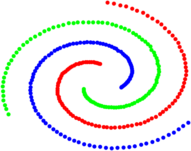
(a) Original

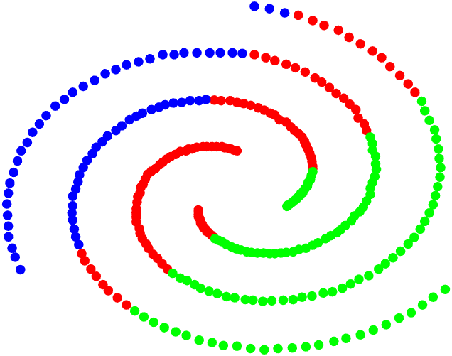
(b) LRR

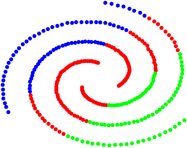
(c) NSLLRR

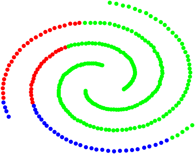
(d) AWLRR

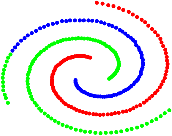
(e) LRRAGR

(f) RSEC

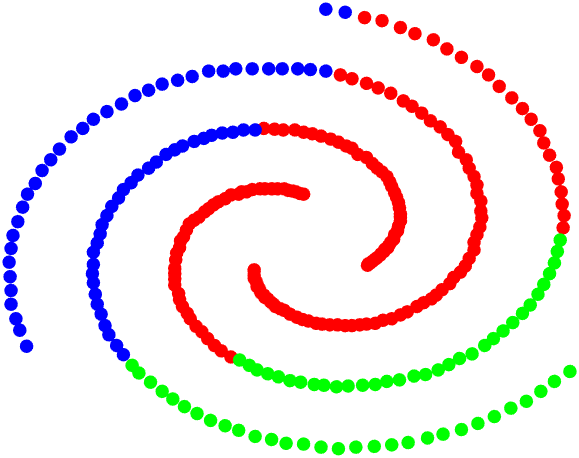
(g) LapNR

(h) ALRR

Figure 1: Experimental results on the spiral database.

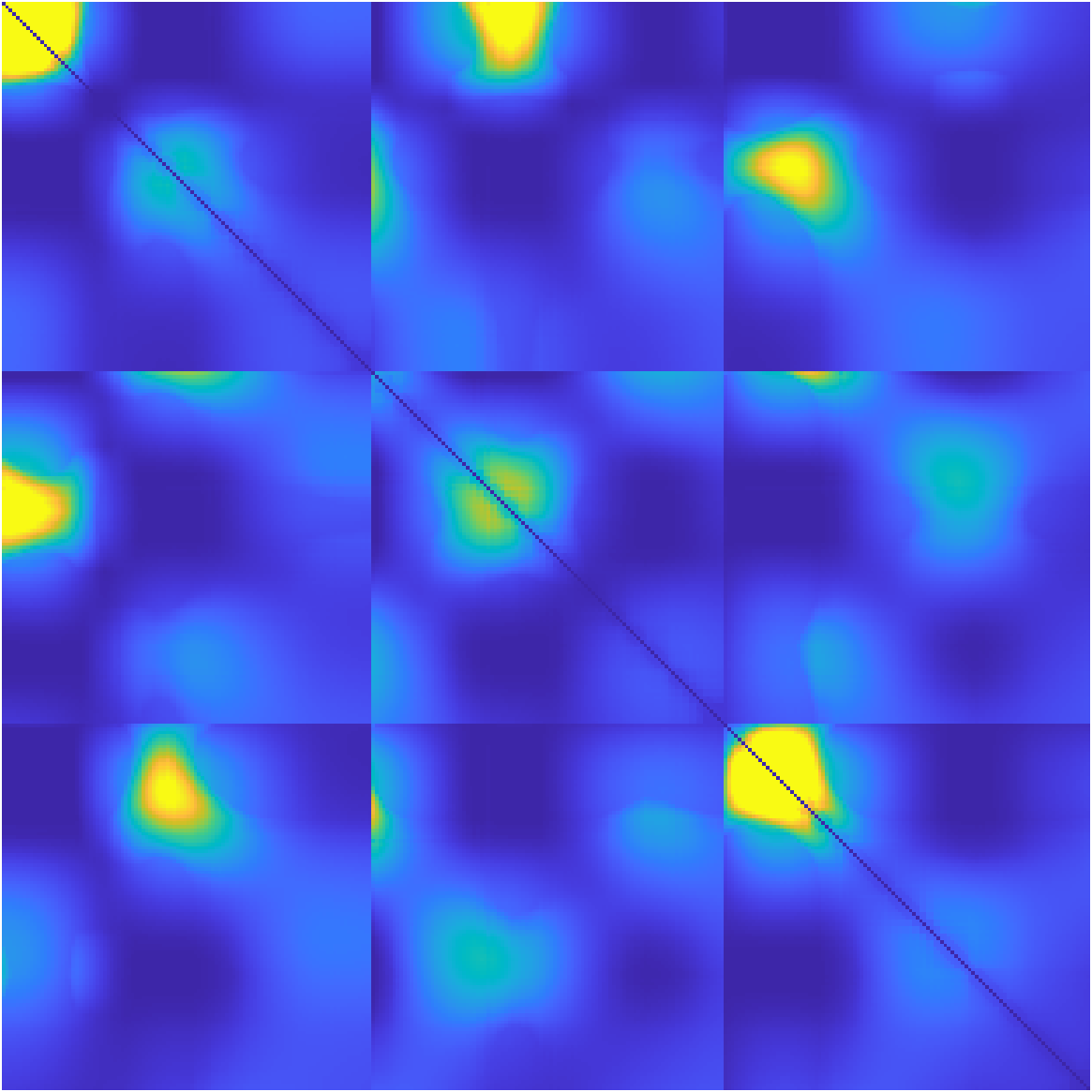
(a) LRR

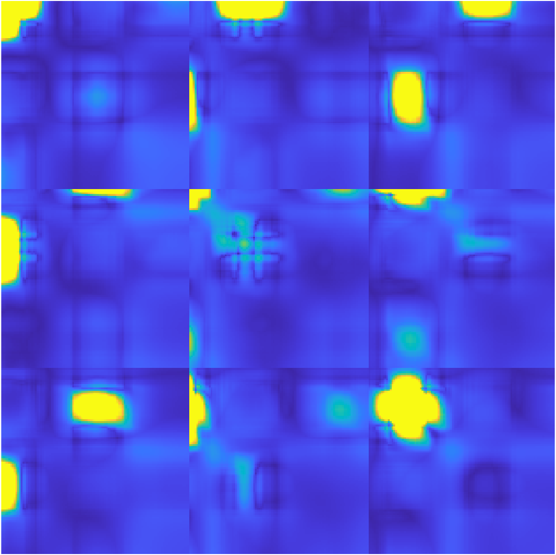
(b) NSLLRR

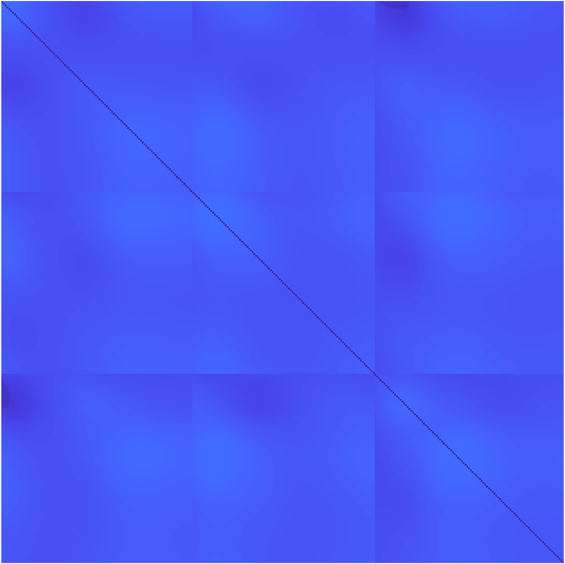
(c) AWNLRR

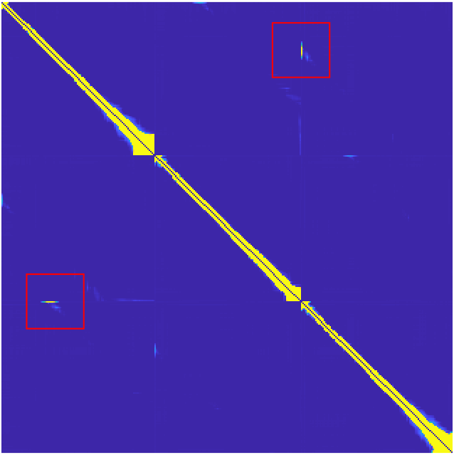
(d) LRRAGR

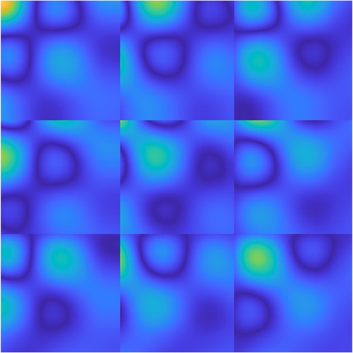
(e) RSEC

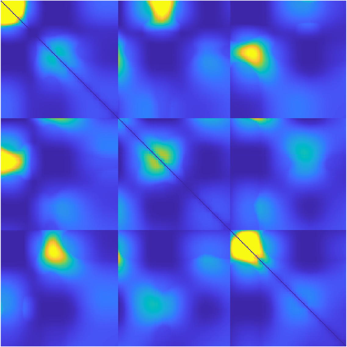
(f) LapNR

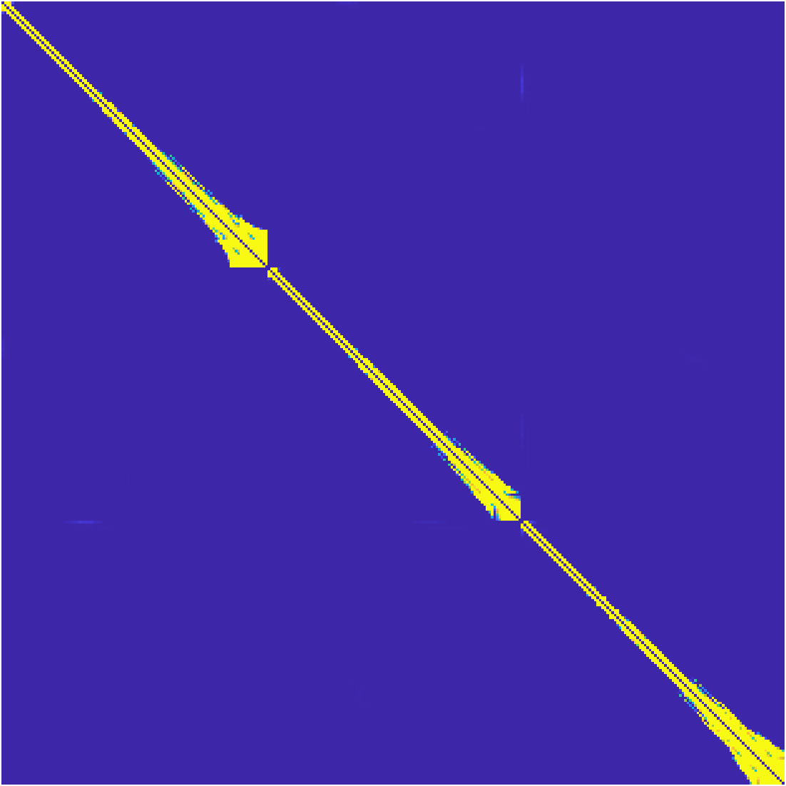
(g) ALRR

Figure 2: Visual comparison of the SGs of LRR, NSLLRR, AWNLRR, RSEC, LapNR, HWLRR and our ALLR.

In this subsection, the computational complexity is analysed firstly. As shown in Algorithm 1, solving the proposed method contains six main steps, i.e., step 1 to step 1. Here, the computational complexity of each step is analysed respectively. Step 1 is updated as Eq.(6) in which $(X^{T}X+2I)^{-1}$ costs the most computational complexity, and its computational complexity is $\mathcal{O}(n^{3})$. However, this term can be pre-calculated to reduce the computational complexity. Steps 1 and 1 use singular value thresholding (SVT) and eigen-decomposition respectively, thus the computational complexity of them are $\mathcal{O}(n^{3})$ and $\mathcal{O}(cn^{2})$, where $c$ is the number of learned rank. The computational complexity of step 1 and 1 is $\mathcal{O}(n^{2})$. Since the computational complexities of basic matrix operations are much lower, these computational complexities are not taken into account. Finally, the computational complexity of the proposed method is $\mathcal{O}(\tau(n^{3}+(c+2)n^{2}))$, where $\tau$ is the number of iteration.

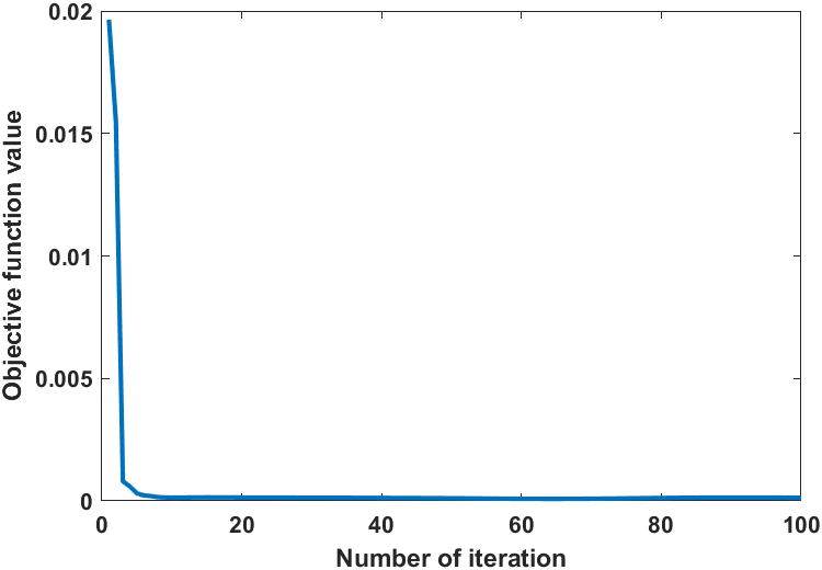
(a) Cars

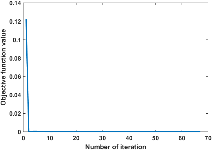
(b) Control

Figure 3: Convergence curve of our ALRR on Cars and Control, in which all classes of each database are selected.

The proposed method is solved by ADMM-style method with six blocks. The strongly convex of two-block ADMM method has been proved in Lin et al. (2015). However, it is still hard to prove that a six-block ADMM method is convex. Hence, we prove the convergence of ALRR by experiments in the following. As shown in Fig.3, the value of the objective function, i.e., $\text{Obj}=(\sum_{i,j}\|Ax_{i}-Ax_{j}\|_{2}^{2}z_{i,j}+\lambda_{1}\|Z\|_{*}+\lambda_{2}\|E\|_{1}+\lambda_{3}\langle L_{Z},Y\rangle)/\|X\|_{F}$, will monotonically decreasing and finally arriving the local optimum, which can show the convergence of ALRR.

4 Experiments

In this section, some experiments are conduceted to show the effectiveness of our ALRR method. Here, some self-representation methods, i.e., LRR, NSLLRR Yin et al. (2016), AWNLRR Wen et al. (2018b), LRRAGR Wen et al. (2018a), RSEC Tao et al. (2019) and LapNR Zhao et al. (2020) are chosen as the comparison algorithms. To make it fair, the parameters of each method are varied in a wide range to obtain the optimum performance. Moreover, the SGs obtained by these methods are symmetrized by $W=(|Z|+|Z|^{T})/2$ and $W$ is handled by Ncut Shi and Malik (2000) to obtain the clustering result. In the experiments, a synthetic database and some benchmark real databases are used to evaluate the performance of all the methods and the details of these databases are shown in Table 1.

Table 1: Description of the databases

Type	Database	Samples	Dim	Classes
Synthetic	Spiral	393	2	3
UCI	Cars	392	8	3
	Contral	600	60	6
	Isolet	1560	617	2
	Solar	323	12	6
	Yeast	1484	1470	10
Handwritten	Dig	1797	64	10
	USPS	1000	256	10
Face	Jaffe	213	676	10
	Yale	165	1024	15
	EYB*	2414	1024	38

• EYB denotes Extended Yale B.

4.1 Clustering on synthetic database

Table 2: Clustering results on real databases

Database	Metric	Cars	Control	Isolet	Solar	Yeast	Dig	USPS	Jaffe	Yale	EYB
Ncut	ACC	48.72	51.50	55.58	51.7	32.28	76.85	49.50	89.20	20.00	19.72
LRR		62.76	48.17	55.96	51.39	30.26	79.13	53.30	99.53	46.06	67.44
NSLLRR		63.52	65.00	59.36	54.80	39.22	67.78	54.20	99.53	54.55	38.48
AWNLRR		66.33	53.17	58.40	55.11	10.71	79.86	55.00	98.59	41.84	88.07
LRRAGR		62.76	56.83	54.00	45.51	30.39	59.32	40.90	98.59	56.36	87.04
RSEC		63.01	54.33	62.95	56.04	38.01	79.19	53.80	100	55.15	88.53
LapNR		57.14	37.83	58.65	52.63	39.22	76.02	57.20	98.12	55.15	48.76
ALRR		68.11	74.50	61.47	59.75	44.54	82.80	59.40	100	61.21	99.13
Ncut	Fscore	48.60	58.35	50.62	43.03	38.47	67.71	36.96	82.45	14.43	12.79
LRR		63.17	57.25	50.65	44.82	35.93	72.85	43.82	99.05	28.25	46.18
NSLLRR		63.67	62.11	51.75	45.87	29.39	63.23	42.35	99.03	36.79	13.12
AWNLRR		66.04	53.47	51.53	46.65	28.96	76.90	46.81	97.11	38.57	85.14
LRRAGR		59.25	69.10	51.00	37.84	35.94	45.25	38.90	97.10	38.68	78.63
RSEC		58.92	57.61	53.43	47.81	31.75	72.32	44.33	100	35.07	80.82
LapNR		50.54	54.28	52.24	45.62	29.39	71.70	47.24	96.32	35.40	25.95
ALRR		67.47	75.17	53.98	50.65	32.84	75.19	48.39	100	44.76	98.26

A spiral database Chang and Yeung (2008) shown in Fig.1(a) is used to evaluate the performance of ALRR and the comparison methods. This database contains three clusters, and many samples with different label are close in this synthetic database. Thus, using this database can show the ability of clustering methods handling the nearby samples with different labels. As shown in Fig.2(g), ALRR can correctly divide the samples into three clusters against the misleading of the nearby samples with different labels, and the other methods have assigned wrong labels to some sample. To further show the discrimination of the learned SGs, the SGs obtained by all the self-representation is shown by visualization. Here, all the SGs obtained have been symmetrized by $W=(|Z|+|Z|^{T})/2$. From Fig.2, we can find that LRRAGR can learn a SG with three parts, which performs much better than the other comparison methods. However, the SG learned by LRRAGR contains some similarities among samples with different labels are greater than 0, which can mislead the clustering method and leads to a worse performance. Due to the learned sparse SG with exactly three diagonal blocks, ALRR can achieve the best clustering result.

4.2 Clustering on real databases

In this subsection, some benchmark real databases are used to evaluate the performance of the proposed method and comparision methods. Two most used metrices, i.e., ACC and Fscore, are utilized to compare the performance of the final clustering results.

The experimental results on these real databases are given in Table 2, and we can find some conclusions as follows.

• Overall, the proposed ALRR outperforms the comparison methods on most databases and can obtain competitive results on the other databases, which can prove the effectiveness of ALRR. Specifically, for the databases with more dimensions, e.g., EYB and Yale, ALRR performs much better than the other methods which prove that the proposed method is more effective on the high-dimensional database. This is because high-dimensional data contains more redundant features, and the auto-weighted matrix can enlarge the effect of the discriminative features.

• Compared with LRR, NSLLRR, LRRAGR, AWNLRR, HWLRR and ALRR perform better in the most cases. Since LRR just uses a global low-rank constraint to capture the global, NSLLRR, AWNLRR, HWLRR and ALRR improve the LRR by preserving more local structure. Thus, it is obvious that learning the local structure is effective for clustering task.

• From the comparison among AWNLRR, LRRAGR and ALRR, we can find that ALRR obtains higher accuracy. These three methods use the distance penalty to learn more geometric structure, but ALRR uses an auto-weighted penalty to enlarge the effect of the disciminative features, which leads to a better SG.

• LRRAGR and ALRR both take use of the class information. LRRAGR utilizes the class information by a rank constraint, and ALRR ensures that the learned SG contains $k$ diagonal blocks. Hence, this can prove that the block constraint is more effective than the rank constraint for clustering.

From these analyses, the effectiveness of the auto-weighted penalty and the block constraint have been proved. With the integration of above factors, the proposed ALRR performs better than the other methods.

4.3 Effectiveness of the auto-weighted matrix

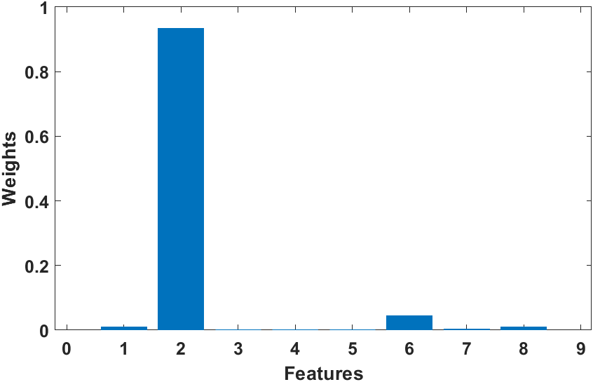
(a) Cars

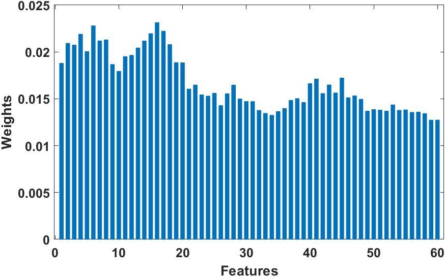
(b) Control

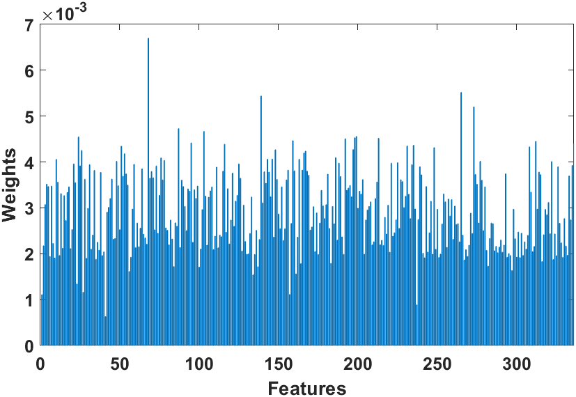
(c) Ecoli

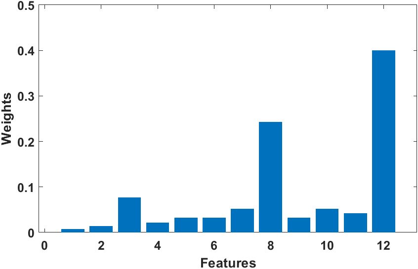
(d) Solar

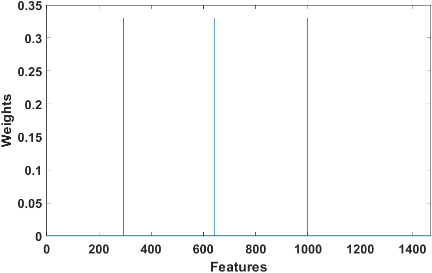
(e) Yeast

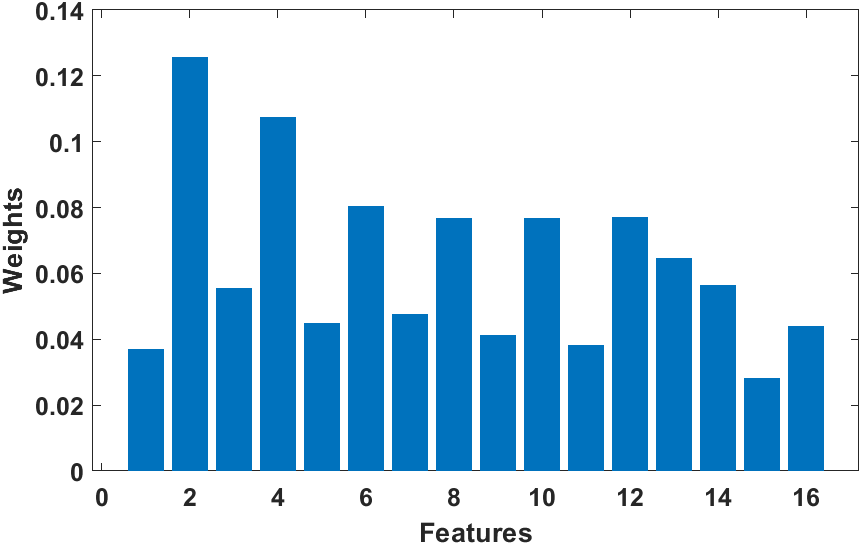
(f) PD

Figure 4: The learned weights of the databases.

Table 3: Clustering results on original and weighted features

	Cars	Control	Isolet	Solar	Yeast	Dig	USPS	Jaffe	Yale	EYB
Original	66.82	59.00	59.32	56.54	41.58	78.50	53.80	98.59	57.58	80.36
Weighted	68.11	74.50	61.47	59.75	44.54	82.80	59.40	100	61.21	99.13

To further show the effectiveness of the auto-weighted matrix, some learned auto-weighted matrix are shown in Fig.4. It can seen that the weights of different features are different, and the weights are adaptively assigned as 1) if the database just contains a few discriminitive features (e.g., Cars and Yeast), the auto-weighted matrix will just select the most important features and remove the useless features; 2) for the database with all the features useful (e.g., Control and PD), the auto-weighted matrix can assign more reasonable weights to enhance the features. Furthermore, we show the contribution of the auto-weighted matrix in our method by setting the auto-weighted matrix $A=I$ in ALRR. As shown in Table 3, the clustering results on the weighted features are better than that on the original features, which shows the effectiveness of the auto-weighted penalty.

4.4 Parameter sensitivity and selection

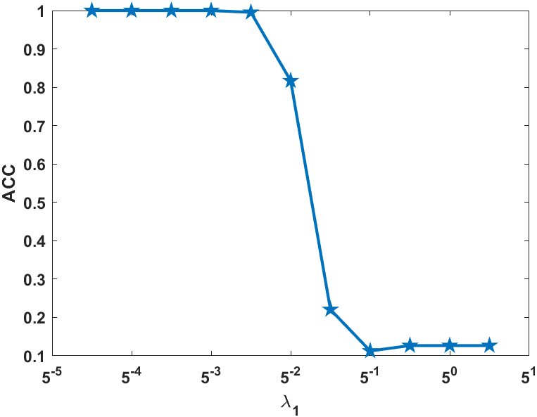
(a) $\lambda_{1}$

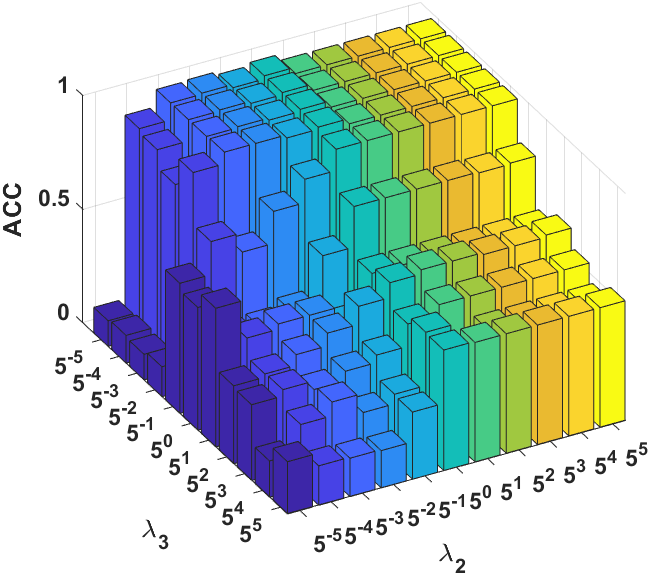
(b) $\lambda_{2}$ and $\lambda_{3}$

Figure 5: Parameter sensitivity analysis of ALRR on the Jaffe, where (a) fix $\lambda_{2}$ and $\lambda_{3}$ to tune $\lambda_{1}$; (b) fix $\lambda_{1}$ to tune $\lambda_{2}$ and $\lambda_{3}$.

As shown in model (3), there are three parameters, i.e., $\lambda_{1}$, $\lambda_{2}$ and $\lambda_{3}$ in the ALRR. They are used to balance the effect of low-rank constraint, error and block constraint, respectively. In this section, the sensitivity of each parameter is tested by performing the proposed method with different combinations of three parameters, and each parameter is varied in a wide range $[5^{-5},5^{-4},...,5^{4},5^{5}]$. First, we fix $\lambda_{2}=5^{-2}$ and $\lambda_{3}=5^{-2}$ to tune $\lambda_{1}$, and thus the sensitivity of $\lambda_{1}$ is shown as Fig.5(a). It is obvious that ALRR can deliver good results with $\lambda_{1}\leq 5^{-1}$. Then, $\lambda_{1}$ is fixed as $5^{-2}$, and the influence of $\lambda_{2}$ and $\lambda_{3}$ is showed by performing the proposed method with different combinations of $\lambda_{2}$ and $\lambda_{3}$ on the Jaffe database. As shown in Fig.5(b), we can find that ALRR performs well with $\lambda_{2}\leq 5^{-2}$ and $\lambda_{3}\leq 5^{-2}$. Since finding a suitable combination of parameters is still an open problem, and we just confirm that the most suitable parameters in our method can be found in a small range, i.e., $[5^{-5},5^{-4},5^{-3},5^{-2}]$.

5 Conclusion

In this paper, a novel and unsupervised self-representation learning method, i.e., Auto-weighted Low-Rank Representation (ALRR), is proposed. Our ALRR can learn a discriminative SG which contains $k$ diagonal blocks which is a clear clustering structure. With the guidness of this term, the auto-weighted penalty can adaptively assign different weights to the features which can enlarge the effect of the useful features and reduce the impact of the useless features. Moreover, this penalty can preserve more local structure with the weighted features. The effectiveness of our ALRR for clustering has been examined on both synthetic and real databases.

References

- Belkin and Niyogi [2008] Mikhail Belkin and Partha Niyogi. Towards a theoretical foundation for laplacian-based manifold methods. J. Comput. Syst. Sci., 74(8):1289–1308, 2008.
- Chang and Yeung [2008] Hong Chang and Dit-Yan Yeung. Robust path-based spectral clustering. Pattern Recognit., 41(1):191–203, 2008.
- Fei et al. [2017] Lunke Fei, Yong Xu, Xiaozhao Fang, and Jian Yang. Low rank representation with adaptive distance penalty for semi-supervised subspace classification. Pattern Recognit., 67:252–262, 2017.
- Feng et al. [2014] Jiashi Feng, Zhouchen Lin, Huan Xu, and Shuicheng Yan. Robust subspace segmentation with block-diagonal prior. In IEEE CVPR, pages 3818–3825, 2014.
- He et al. [2011] Ran He, Wei-Shi Zheng, Bao-Gang Hu, and Xiangwei Kong. Nonnegative sparse coding for discriminative semi-supervised learning. In IEEE CVPR, pages 2849–2856, 2011.
- Lin et al. [2011] Zhouchen Lin, Risheng Liu, and Zhixun Su. Linearized alternating direction method with adaptive penalty for low-rank representation. In NeurIPS, pages 612–620, 2011.
- Lin et al. [2015] Zhouchen Lin, Risheng Liu, and Huan Li. Linearized alternating direction method with parallel splitting and adaptive penalty for separable convex programs in machine learning. Mach. Learn., 99(2):287–325, 2015.
- Liu et al. [2010] Guangcan Liu, Zhouchen Lin, and Yong Yu. Robust subspace segmentation by low-rank representation. In ICML, pages 663–670, 2010.
- Liu et al. [2012] Guangcan Liu, Huan Xu, and Shuicheng Yan. Exact subspace segmentation and outlier detection by low-rank representation. In AISTATS, volume 22, pages 703–711, 2012.
- Liu et al. [2013] Guangcan Liu, Zhouchen Lin, Shuicheng Yan, Ju Sun, Yong Yu, and Yi Ma. Robust recovery of subspace structures by low-rank representation. IEEE TPAMI, 35(1):171–184, 2013.
- Lu et al. [2019] Canyi Lu, Jiashi Feng, Zhouchen Lin, Tao Mei, and Shuicheng Yan. Subspace clustering by block diagonal representation. IEEE TPAMI, 41(2):487–501, 2019.
- Shah and Koltun [2017] Sohil Atul Shah and Vladlen Koltun. Robust continuous clustering. Proc. Natl. Acad. Sci. USA, 114(37):9814–9819, 2017.
- Shi and Malik [2000] Jianbo Shi and Jitendra Malik. Normalized cuts and image segmentation. IEEE TPAMI, 22(8):888–905, 2000.
- Song and Wu [2018] Yu Song and Yiquan Wu. Subspace clustering based on latent low rank representation with frobenius norm minimization. Neurocomputing, 275:2479–2489, 2018.
- Tao et al. [2019] Zhiqiang Tao, Hongfu Liu, Sheng Li, Zhengming Ding, and Yun Fu. Robust spectral ensemble clustering via rank minimization. ACM TKDD, 13(1):1–25, 2019.
- Wang et al. [2020] Rong Wang, Haojie Hu, Fang He, Feiping Nie, Shubin Cai, and Zhong Ming. Self-weighted collaborative representation for hyperspectral anomaly detection. Signal Process., 177:107718, 2020.
- Wen et al. [2018a] Jie Wen, Xiaozhao Fang, Yong Xu, Chunwei Tian, and Lunke Fei. Low-rank representation with adaptive graph regularization. Neural Networks, 108:83–96, 2018.
- Wen et al. [2018b] Jie Wen, Bob Zhang, Yong Xu, Jian Yang, and Na Han. Adaptive weighted nonnegative low-rank representation. Pattern Recognit., 81:326–340, 2018.
- Wen et al. [2021] Jie Wen, Zheng Zhang, Zhao Zhang, Lei Zhu, Lunke Fei, Bob Zhang, and Yong Xu. Unified embedding alignment with missing views inferring for incomplete multi-view clustering. In AAAI, page early access, 2021.
- Yang et al. [2020] Jufeng Yang, Jie Liang, Kai Wang, Paul L. Rosin, and Ming-Hsuan Yang. Subspace clustering via good neighbors. IEEE TPAMI, 42(6):1537–1544, 2020.
- Yin et al. [2016] Ming Yin, Junbin Gao, and Zhouchen Lin. Laplacian regularized low-rank representation and its applications. IEEE TPAMI, 38(3):504–517, 2016.
- Zhang et al. [2018a] Xingxing Zhang, Zhenfeng Zhu, Yao Zhao, and Dongxia Chang. Learning a general assignment model for video analytics. IEEE TCSVT, 28(10):3066–3076, 2018.
- Zhang et al. [2018b] Xingxing Zhang, Zhenfeng Zhu, Yao Zhao, and Deqiang Kong. Self-supervised deep low-rank assignment model for prototype selection. In IJCAI, pages 3141–3147, 2018.
- Zhang et al. [2019] Xingxing Zhang, Zhenfeng Zhu, Yao Zhao, Dongxia Chang, and Ji Liu. Seeing all from a few: -norm-induced discriminative prototype selection. IEEE TNNLS, 30(7):1954–1966, 2019.
- Zhao et al. [2020] Y. Zhao, L. Chen, and C. L. P. Chen. Laplacian regularized nonnegative representation for clustering and dimensionality reduction. IEEE TCSVT, early access, 2020.