StegaPos: Preventing Unwanted Crops and Replacements
with Imperceptible Positional Embeddings

Abstract

We present a learned, spatially-varying steganography system that allows detecting when and how images have been altered by cropping, splicing or inpainting after publication. The system comprises a learned encoder that imperceptibly hides distinct positional signatures in every local image region before publication, and an accompanying learned decoder that extracts the steganographic signatures to determine, for each local image region, its 2D positional coordinates within the originally-published image. Crop and replacement edits become detectable by the inconsistencies they cause in the hidden positional signatures. Using a prototype system for small $(400\times 400)$ images, we show experimentally that simple CNN encoder and decoder architectures can be trained jointly to achieve detection that is reliable and robust, without introducing perceptible distortion. This approach could help individuals and image-sharing platforms certify that an image was published by a trusted source, and also know which parts of such an image, if any, have been substantially altered since publication.

1 Introduction

Any image that is shared online is subject to a risk of tampering, because instead of re-sharing a faithful copy of the original, an adversary can share an altered version that has had some pixels replaced with other content (via inpainting or splicing) or that has been cropped to change its meaning (e.g., [13, 2]). The widespread possibility of such tampering creates a fundamental lack of trust: When viewing an image online, an observer cannot know whether it is a faithful rendition of the creator’s original intent.

In the past it has been possible to detect crop, splice and inpainting alterations from the subtle inconsistencies they produced, such as implausible semantic layouts, inconsistencies in lighting or color tone, and inconsistencies in spatial noise patterns (e.g., [37, 32, 12, 33, 26]). But the utility of these approaches has quickly diminished with the rise of modern tampering techniques and AI-based generation technology, which can increasingly replace and create pixels with very few measurable inconsistencies.

We present a new approach for reducing the risk of tampering based on learned steganography. As in conventional deep watermarking and steganography (e.g., [4, 10, 25]), we train an encoder network to embed imperceptible information into an image, and we train an accompanying decoder network to retrieve the information. But instead of embedding one message globally into an image, we design our networks to embed and retrieve distinct information in every local region. This allows detecting which parts of an image are missing (due to cropping) and which parts have been replaced (due to splicing or generative inpainting).

One way to deploy our networks would be to host them on a secure server or on confidential computing hardware. Trusted content creators—such as journalists, photographers and digital artists—could be authorized to encode their images through an API before publishing them online. Then, upon receiving an image, any individual or image-sharing platform could submit a regulated query to the decoder to determine: (i) whether the image can be certified as having originated from the authorized pool of creators; and if so, (ii) which parts of the image, if any, have been substantially altered since publication.

We call our system StegaPos because the information that it steganographically embeds within each local image region is an encoding of that region’s 2D position within the original image. The decoder is trained to recover the hidden positional field by analyzing each local image region, which allows crops and replacements to be detecting from the disturbances they cause in the hidden positional field. Using a large collection of small $(400\times 400)$ images, we provide a proof-of-concept demonstration that it is possible to implement this approach using relatively simple CNNs. By training them jointly, we create an encoder-decoder pair that imperceptibly provides useful detection capabilities. In particular, we show these capabilities can be made to robustly survive through common distortions—such as tone-adjustment and resizing—that may be deemed socially “allowable” to facilitate convenient sharing between diverse devices without substantially altering the creator’s intent.

Our experiments show quantitatively that our model provides competitive performance across a range of existing benchmarks for splice detection, as well as on a new benchmark for crop detection.

2 Related Work

Reactive methods for splice and crop detection are different from ours because they do not require proactively embedding protective information into an image before it is published. Instead, they react by detecting flaws in a tamperer’s work, such as inconsistencies in lighting, shadows, tone mapping, sensor noise signatures, and optical signatures like vignetting. The best reactive methods use deep networks that are trained on large datasets of example splices [37, 32, 12] or crops [26], and compared to our approach, they have the important advantage of being applicable to legacy online images that were not proactively protected. However, any reactive approach is fundamentally in an arms race with counter-forensic methods, which can use increasingly sophisticated processing to eliminate their flaws [8]; and recent advances in AI-based image generation suggest this forensic arms race may soon be lost.

We show experimentally that our proactive approach improves accuracy on existing splice-detection benchmarks compared to reactive techniques, and we further show that we can detect splices—and crops—when absolutely no inconsistencies are present.

Deep watermarking and deep steganography use learned encoder and decoder networks to imperceptibly hide a bit-string in an image by modifying its pixel values. This can can be used to broadcast a supplemental piece of information, such as a URL or ownership label [24, 38, 35, 29, 31, 10], or to transmit a covert message that is unnoticeable to adversaries [38]. One often wants to build redundancy into the encoding, so that the string can survive through distortions of the host image that may occur during transmission and sharing, such as downsampling, JPEG compression, or re-imaging after projection or printing. An established way to achieve such robustness is to include simulated distortions between the encoder and decoder during training [24, 30, 3]. We find that our networks provide reasonable robustness towards common distortions without augmented training so we leave this for future work.

At a basic level, any watermarking or steganographic system must strike a balance between: (i) the amount of hidden information, (ii) the perceptible distortion it creates, and (iii) its ability to survive distortions [6]. The existing work has explored learning this balance when a single message is being embedded across all of an image’s pixels. In contrast, we explore learning this balance when the message is spatially-varying, meaning that distinct information is being hidden in every local region.

Block-level protection refers to a class of watermarking techniques that are spatially-varying like ours and that can also protect against replacement alterations. These techniques are cleverly engineered instead of learned. They typically operate by partitioning an image into blocks and modifying some of the bits to embed inter-block signatures that allow detecting when blocks are modified, and furthermore allow recovering contents in the modified blocks (e.g., [16, 17, 18]). These methods can be very effective (see the supplement for an example) but they are extremely sensitive to distortions like compression and downsampling [5], which can limit their utility for practical sharing across devices. Our learning-based approach has a different motivation. It forgoes the ability to reconstruct content that has been modified, and it instead focuses on finding a balance between robustness, protection, and imperceptibility.

Digital signatures use encryption to attach metadata to an image that allows the recipient to know who created it (attribution) and to know that it has not been altered in transit (exact integrity). Our system serves a different purpose. It is designed to support attribution to an authorised pool of creators, but not to a specific individual within the pool. Also, instead of indicating exact integrity, it provides a softer indication of authenticity to the creator’s intent. This has the advantages of being able to survive through distortions like downsampling that are common to online sharing, and it also provides richer information about where and how an image has been altered since publication.

3 Steganographic Positional Embedding

Our system is shown in Figure 1. A color image $I(x,y,c)\in[0,1]$ of size $H\times W\times 3$ is input to a CNN $\tilde{f}_{\theta}$ which generates a signal $\gamma(x,y,c)$ of the same size. The signal is added (with clamping) to create an encoded image $\hat{I}$ that is perceptually close to $I$. We call $\hat{I}$ a steganographic-positional image, or stegapos image for short. It is meant to contain, within each local image patch, sufficient information about the spatial position $p=(x,y)\in\{1\ldots W\}\times\{1\ldots H\}$ of the patch’s center.

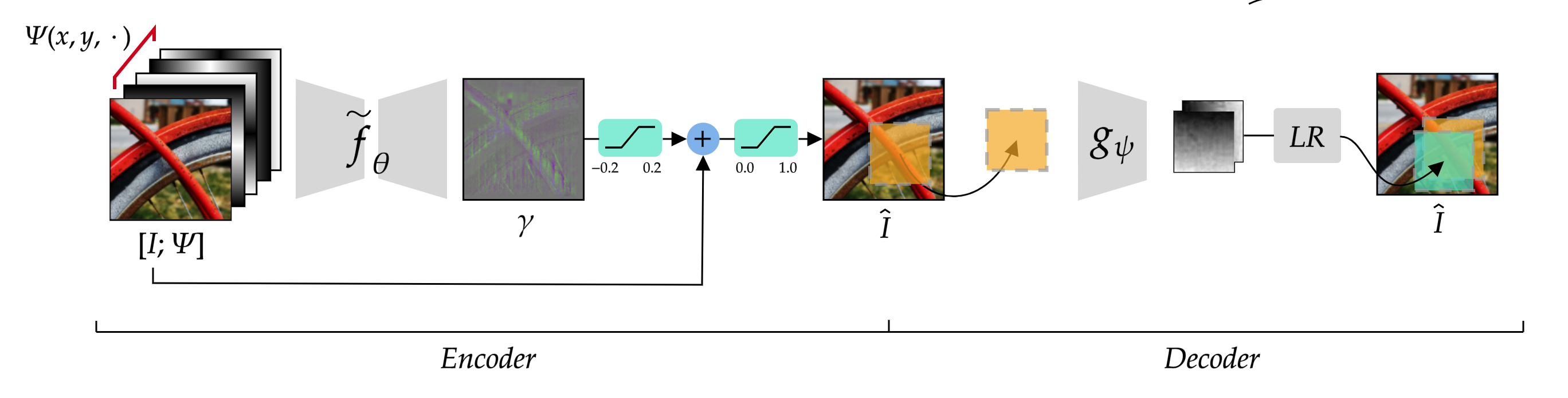
Figure 1: System overview. The encoder concatenates input image $I(x,y)$ with frequency-based positional codes $\Psi(x,y,\cdot)$ and maps these to a residual signal $\gamma(x,y)$ that is added to $I$ (with clamping) to produce stegapos image $\hat{I}$. The decoder receives a (possibly cropped and downsampled) image $\hat{I}(i,j)$ and maps this to an array of 2D positions $p(i,j)$ representing the pixel coordinates at which the content at $(i,j)$ was located within the originally-encoded image. The decoded positional field $p(i,j)$ is sufficient to determine whether the input $\hat{I}$ is stegapos-encoded, and if so, which regions have been altered by replacements. Additionally, by passing the field to a subsequent linear regression operator (LR, see Eq. 7), the system infers the top-left offset of a crop and/or a downsampling factor.

Later, when a stegapos image $\hat{I}(i,j,c)\in[0,1]$ arrives at the decoder, possibly after being cropped or downsampled to a different size, a CNN $g_{\psi}$ maps it to an array of inferred position values $p(i,j)\in[1,W]\times[1,H]$, and then a linear regression operator (LR) estimates from $p(i,j)$ a decimation scale-factor and the top-left offset of a crop.

The overarching idea is very simple. In the absence of any splicing, cropping or downsampling, the decoder’s network $g_{\psi}$ should recover from $\hat{I}$ a positional field that is close to the one that was embedded: $p(i,j)\approx(i,j)\ \forall(i,j)\in\{1\ldots W\}\times\{1\ldots H\}$. If there is cropping or downsampling applied to $\hat{I}$, the recovered positional field will also be cropped or downsampled, and this will be detected by the linear regression operator. Moreover, if there is a replacement applied to $\hat{I}$, it causes an anomaly in the positional field (e.g., Figure 2) that can also be detected.

In what follows, our prototype system assumes that all of the encoded images are of a single, pre-determined size ($H\times W$), and that images sent to the decoder are of equal size or smaller. Extensions to larger and variable image sizes are left for future work.

3.1 Encoding

We use a standard U-Net [19, 22] for $\tilde{f}_{\theta}$ with input that is a channel-wise concatenation of the image $I$ and an $H\times W\times D$ array of frequency-based positional codes,

$$\Psi(x,y,\cdot) =\left\{\begin{bmatrix}\cos(\omega_{k}x)\\ \sin(\omega_{k}x)\\ \cos(\omega_{k}y)\\ \sin(\omega_{k}y)\end{bmatrix}\mid\omega_{k}=\omega_{o}^{4k/D},k=1\ldots\tfrac{D}{4}\right\},$$

with frequencies $\omega_{k}$ forming a geometric progression from sufficiently small base frequency $\omega_{o}$. In our experiments we use dimension $D=8$ and follow [27] by using base frequency $\omega_{o}=10^{-4}$.

The CNN output is then clamped and added to the input image according to

$$\gamma =\tilde{f}_{\theta}(\begin{bmatrix}I;\Psi\end{bmatrix})$$ (1)

$$\hat{I} =\text{clamp}_{[0,1]}(I+\text{clamp}_{[-0.2,0.2]}(\gamma)).$$ (2)

We use notation $\hat{I}=f_{\theta}(I)$ for the complete mapping from input to stegapos output.

The frequency-based codes $\Psi$ play an important role and are a convenient input for several reasons. In addition to having values in $[-1,1]$ and providing a unique $D$-dimensional signature at each position $(x,y)$, they provide the CNN with a range of input spatial frequencies that it can mix to create local residuals that “match” (in a perceptual sense) the various local textures and colors of an input image. The codes also have a linear and shift-invariant relational property, meaning that codes $\Psi(x,y,\cdot)$ and $\Psi(x+\Delta x,y+\Delta y,\cdot)$ are related by a linear transformation (see expression in the supplement) that depends only on $(\Delta x,\Delta y)$. This can help to “work around” smooth, uniformly-colored parts of an input image, which tend to be perceptually sensitive to rapidly-varying residuals, by instead placing information about relative position at nearby points that are less perceptually sensitive.

3.2 Decoding

The decoder receives a color image $\hat{I}(i,j,c)\in[0,1]$ of size $N\times M\times 3,$ with $N\leq W,M\leq H$. We use a standard, undecimated (i.e., stride-$1$) CNN for $g_{\psi}$ to map from the image to its embedded positional field $p(i,j)$. We discard positional estimates near the borders of the image that are affected by windowing, so the CNN’s output is of size $(N-R+1)\times(M-R+1)$, where $R$ is the receptive field size, and its output values $p$ are nominally in the range $[\lfloor\frac{R}{2}\rfloor,W-\lceil\frac{R}{2}\rceil]\times[\lfloor\frac{R}{2}\rfloor,H-\lceil\frac{R}{2}\rceil]$.

The receptive field $R$ is determined by the CNNs filters and layers and is a critical design parameter. Larger receptive fields allow aggregating positional information about each $(i,j)$ from a larger neighborhood around it, which increases the accuracy of the positional estimates and, perhaps more importantly, increases the local information capacity that is available to the encoder for embedding positional information with less perceptual distortion. On the other hand, smaller receptive fields increase the spatial precision of the positional estimates, allowing the detection of positional aberrations (due to crops or splices) that are smaller in size. In our experiments, we use $R=50$, which is $12.5\%$ of the image width.

The network $g_{\psi}$ is trained, via augmentation as described below, to be approximately decimation-equivariant. That is, if $p=g_{\psi}(I)$ and $q=g_{\psi}(I_{\downarrow_{1/s}})$ for some decimation factor $s\in\left[s_{\text{min}},1\right]$ in a pre-determined range, then the two outputs are related by $p_{\downarrow_{1/s}}\approx q$. This ensures that hidden positional signatures can be recovered in spite of downsampling that occurs between encoding and decoding, and, as a by-product, it also allows detecting when a stegapos image has been downsampled and by how much.

The linear regression operator accepts the estimated positional field $p(i,j)=(p_{x}(i,j),p_{y}(i,j))$ and analytically computes least squares estimates of the decimation scale factor and the top-left coordinates of a crop. An image cropped with top-left offset $(\mu_{x},\mu_{y})\in[1,W]\times[1,H]$ and scaled by $s\in\left[s_{\text{min}},1\right]$ will have ideal CNN outputs

$$\mathcal{P}^{([\mu_{x},\mu_{y}],s)}_{x}(i,j)\triangleq\mu_{x}+(\lfloor{\tfrac{R}{2}}\rfloor+i)\tfrac{1}{s}$$ (3)

$$\mathcal{P}^{([\mu_{x},\mu_{y}],s)}_{y}(i,j)\triangleq\mu_{y}+(\lfloor{\tfrac{R}{2}}\rfloor+j)\tfrac{1}{s},$$ (4)

so the linear regression operator estimates the offset ($\mu_{x}$, $\mu_{y}$) and scale $s$ via

$$\hat{\mu}_{x},\hat{s}_{x} =\sum_{ij}\text{arg}\min_{\mu_{x},s}||p_{x}(i,j)-\mathcal{P}^{([\mu_{x},\mu_{y}],s)}_{x}(i,j)||_{2}^{2}$$ (5)

$$\hat{\mu}_{y},\hat{s}_{y} =\sum_{ij}\text{arg}\min_{\mu_{y},s}||p_{y}(i,j)-\mathcal{P}^{([\mu_{x},\mu_{y}],s)}_{y}(i,j)||_{2}^{2}$$ (6)

$$\hat{s} =\frac{\hat{s}_{x}+\hat{s}_{y}}{2}.$$ (7)

Note that $\mathcal{P}^{([0,0],1)}$ is the expected CNN output for an image that has not been cropped or scaled. Also note that it would be possible to separately estimate $\hat{s}_{x}$ and $\hat{s}_{y}$ in order to detect scalings of aspect ratio.

3.3 Training

We train the system end-to-end with a loss that simultaneously promotes positional accuracy and visual fidelity:

$$\begin{split}\mathcal{L}(\theta,\psi,\phi)&=||p-\mathcal{P}^{([0,0],s)}_{x,y}||_{2}^{2}+\lambda_{\gamma}||\gamma||_{1}\\ &+\lambda_{I}||\hat{I}_{YUV}-I_{YUV}||_{1}+\lambda_{s}\mathcal{L}_{s}(I,\hat{I})\\ &-\lambda_{c}\log d_{\phi}(f_{\theta}(I))\end{split}$$ (8)

Here, $\gamma=\tilde{f}_{\theta}(I)$ is the residual image, $\hat{I}=f_{\theta}(I)$ is the encoded image, $p=g_{\psi}(f_{\theta}(I))$ is the decoded positional field, and $I_{YUV}$ is an image converted to YUV color space. $\mathcal{L}_{s}(I,\hat{I})$ is a perceptual loss [36], and the final term, with weight $\lambda_{c}$, is a critic loss that employs an auxiliary CNN discriminator $d_{\phi}:\{I\}\mapsto[0,1]$ with weights $\phi$ that adapt to differentiate between input and encoded images [15]. We alternate between updating weights $\phi$ to reduce $\mathcal{L}_{D}=-\log d_{\phi}(I)-\log(1-d_{\phi}(\hat{I}))$ and updating weights $\theta,\psi$ to reduce $\mathcal{L}(\theta,\psi)$.

To achieve approximate decimation-equivariance in the decoder, we find it sufficient to use a simple augmentation approach during training: We randomly scale each encoded image by $s\in[s_{\text{min}},1]$ before feeding it to the decoder and then evaluate the positional loss between the outputs $p$ and the expected decimated output $\mathcal{P}^{([0,0],s)}_{x,y}$.

We use a two-phase training regime similar to [24], first training for positional accuracy by setting $\lambda_{I}=\lambda_{c}=\lambda_{s}=\lambda_{\gamma}=0$, and then training for both position and visual quality using all loss terms until convergence. We find the first phase converges quickly with high positional accuracy but low visual quality, and that visual quality restores when the regularization coefficients $\{\lambda_{I},\lambda_{c},\lambda_{\gamma},\lambda_{s}\}$ are gradually increased during the second phase.

4 Experiments

We train using 100,000 images of size $400\times 400$ from the MIRFLICKR 1M dataset. We use dimension $D=8$ with base frequency $\omega_{o}=10^{-4}$ for the input positional codes. The decoder receptive field size is $R=50$, and we train over decimation factors $s\in[0.2,1]$. Architectural details for the three CNNs are in the supplement.

During training, we use a batch size of $8$ images and the Adam optimizer with learning rate $10^{-7}$ and $(\beta_{1},\beta_{2})=(0.9,0.999)$. Overall, we find that training is quite susceptible to poor local minima, and we resort to manual manipulation of coefficients $\{\lambda_{I},\lambda_{c},\lambda_{\gamma},\lambda_{s}\}$ during training.

Figure 2 visualizes a residual signal created by the encoder along with the positional field recovered by the decoder. Figures 3 and 5 show some representative results for applications to crop and replacement detection. Overall, the following experiments show the system is capable of preserving high visual quality while also achieving high positional accuracy. It provides close equivariance with decimation, is robust to several allowable distortions, and enables the detection of splice/replacement masks with useful spatial precision. At the end of this section, in Part 4.5, we provide insight into what the system has learned by examining some statistics of the residual signals created by the encoder.

4.1 Stegapos or not?

We begin with the authentication task of classifying an image as being stegapos-encoded or not. This is useful to an observer who wants to verify the source of the image.

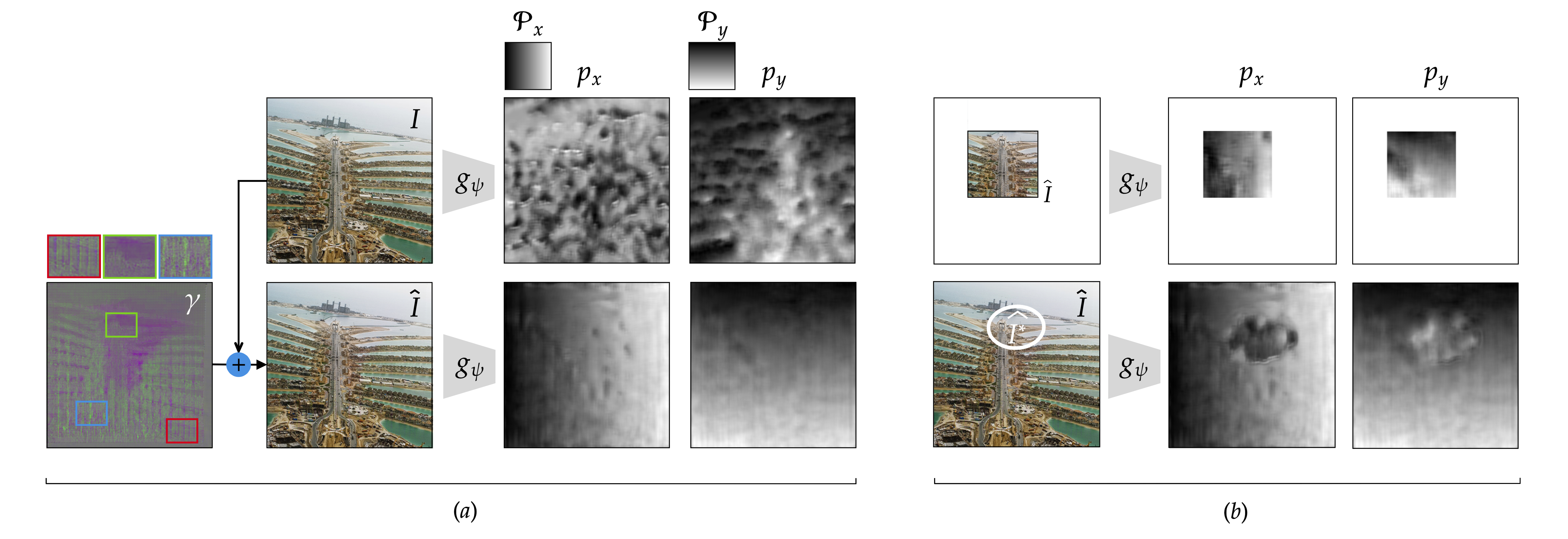
Figure 2: Visualizations of decoded positional fields $p(i,j)=\left(p_{x}(i,j),p_{y}(i,j)\right)$. (a) An unencoded image $I$ maps to a structureless field while an encoded one $\hat{I}$ maps close to smooth positional field $\left({\cal P}_{x},{\cal P}_{y}\right)$ that was embedded. (b) Examples of positional fields decoded after crops or replacements. Anomalies in the field caused by a replacement are detectable even when the replacement is visually perfect. See text for details.

The visualizations in Figure 2(a) suggest that stegapos images $\hat{I}$ can be easily distinguished by the positional estimates $p=g_{\psi}(\hat{I})$ they induce. To verify this, we train a single layer classifier with sigmoid activation that accepts $p(i,j)$ and estimates the probability that $\hat{I}$ is stegapos-encoded. We train and validate the classifier on a 25,000/10,000-split of the original MIRFLICKR 1M dataset, applying stegapos-encoding to half of the images and leaving the rest unencoded. We freeze the encoder and decoder parameters and optimize the classifier weights using the $\ell_{2}$-loss between the estimated and ground-truth binary (encoded/unencoded) labels. The classifier converges quickly and provides $100\%$ training accuracy and $99.4\%$ validation accuracy, from which we conclude that verification of stegapos-encoding is reliably achievable.

4.2 Detecting crops and downsampling

Next we consider the task of estimating the scale and crop-offset of a stegapos image by using the offset and scale estimates $(\hat{\mu}_{x},\hat{\mu}_{y},\hat{s})$ from Equation 7. Figure 3 shows typical results, where the model is able to accurately estimate the cropped regions without sacrificing image quality.

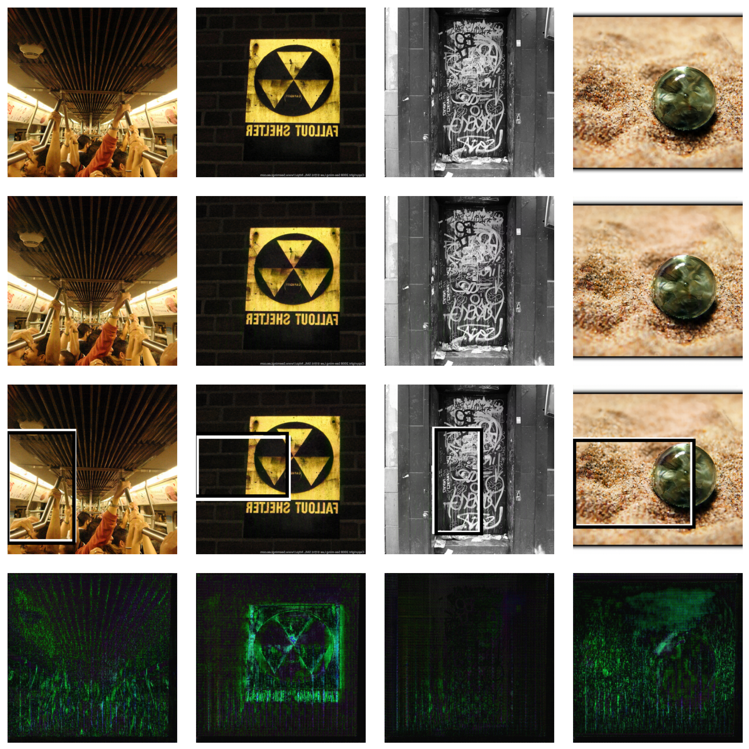
Figure 3: Sample crop detection results ($s=1.0$). (top to bottom) Original image $I$, stegapos image $\hat{I}$, ground truth crop (black) and estimated crop (white), residual image $|\hat{I}-I|$ with values scaled $\times 10$ for visibility.

To quantify accuracy, we build a new dataset we call SmartCrop25K, comprising 25,000 images of size $400\times 400$ from the MIRFLICKR 25K dataset that are cropped at various sizes from full size (no crop) down to $1/16$-size ($50\times 50$ crop). The cropping was done automatically by a saliency-aware system that preserves salient content. Figure 4 visualizes our model’s quantitative results for offset and scale on this dataset.

Crop localization is harder when an image is downsampled ($s<1$) and when the crop retains a smaller fraction of the image. We find that when the input images are not downsampled (first column, $s=1$) the model’s crop offset error is less than 25 pixels for all but the smallest crop sizes. When the images are downsampled (second column) the error degrades in a graceful manner. See the supplement for results on additional values of $s$.

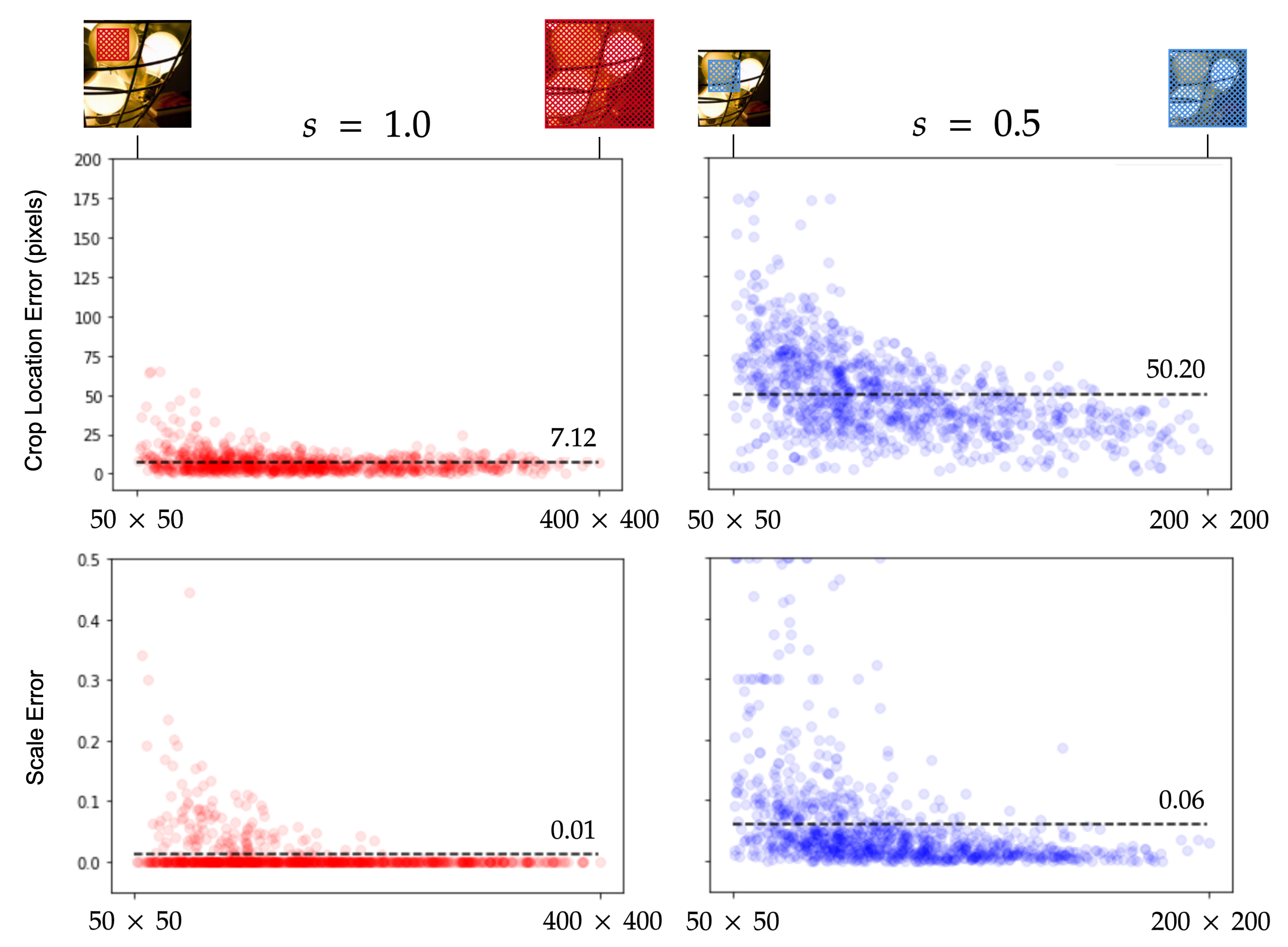
Figure 4: Crop detection errors versus crop size, from $50\times 50$ ($1/16$ crop) to $400\times 400$ (no crop), visualized using 1000 random samples from our 25,000-image dataset. Columns show errors for two scales, $s\in\{1.0,0.5\}$. Top: Error in estimated top-left corner $(\mu_{x},\mu_{y})$, measured in pixels. Bottom: Error in estimated scale $s$. For more complete results, please check the supplement.

4.3 Detecting replacements

Finally, we consider the task of detecting replacements, where a section of a stegapos image has been replaced by pixels from another image or generated content. We quantify performance using examples of two-factor splices, where a composite image $\hat{I}$ has been created by blending content from two different sources according to $\hat{I}(i,j,c)={\cal M}(i,j)\hat{I}_{1}(i,j,c)+(1-{\cal M}(i,j))\hat{I}_{2}(i,j,c)$ with binary mask ${\cal M}\in\{0,1\}$. Our task is to infer the mask ${\cal M}$ from image $\hat{I}$, without prior knowledge of $\hat{I}_{1},\hat{I}_{2}$. There are two cases to consider: (ee) both sources are stegpos-encoded; and (eu) one source is stegapos-encoded and the other source is unencoded.

Figure 2(b) visualizes an artificially-challenging example of the (ee) case, where a composite image is created by copies of itself that are encoded with different relative positions, that is $\hat{I}={(1-\cal M)}f_{\theta}(\hat{I})+{\cal M}f^{\Delta}_{\theta}(\hat{I})$ with $f^{\Delta}$ an encoding from use of phase-shifted input positional codes $\Psi^{\Delta}$. There is absolutely no perceptual evidence for the existence of the replacement, but the anomaly in the recovered positional signature still provides a clear signal for detecting its presence.

The most direct way to estimate mask ${\cal M}$ from input image $\hat{I}$ is to apply a threshold to the per-pixel deviations following the decoder’s linear regression operator, that is

$$\hat{\mathcal{M}}(i,j)=|p(i,j)-\mathcal{P}^{([\hat{\mu}_{x},\hat{\mu}_{y}],\hat{s})}_{x,y}(i,j)|>\alpha,$$ (9)

with some threshold value $\alpha$ and with $\hat{\mu}_{x},\hat{\mu}_{y},\hat{s}$ provided by the linear regression operator. We call this approach “Ours+L” (for linear) in Table 1, and we test situations where (i) the threshold $\alpha$ is fixed across an entire collection of images; and (ii) it is optimally chosen (by an oracle) for each image.

For comparison, we also test a more sophisticated method for splice detection that replaces $g_{\psi}$ with a new U-Net $h_{\phi}$, which maps an (undecimated and uncropped) image $\hat{I}(i,j,c)$ directly to a binary mask $\hat{\cal M}(i,j)$. We call this approach “Ours+N” (for network) in Table 1. We train $h_{\phi}$ using a frozen encoder and a synthetic training set comprising labeled pairs $(\hat{I}^{(i)},{\cal M}^{(i)})$ that are created by combining a 25,000-image subset of the MIRFLICKR 1M dataset with a generated set of simple masks (circles, squares, etc.) using the (ee) scheme. The weights $\phi$ are optimized using loss $||\mathcal{M}-h_{\phi}(\hat{I}))||^{2}_{2}$, and they converge very quickly.

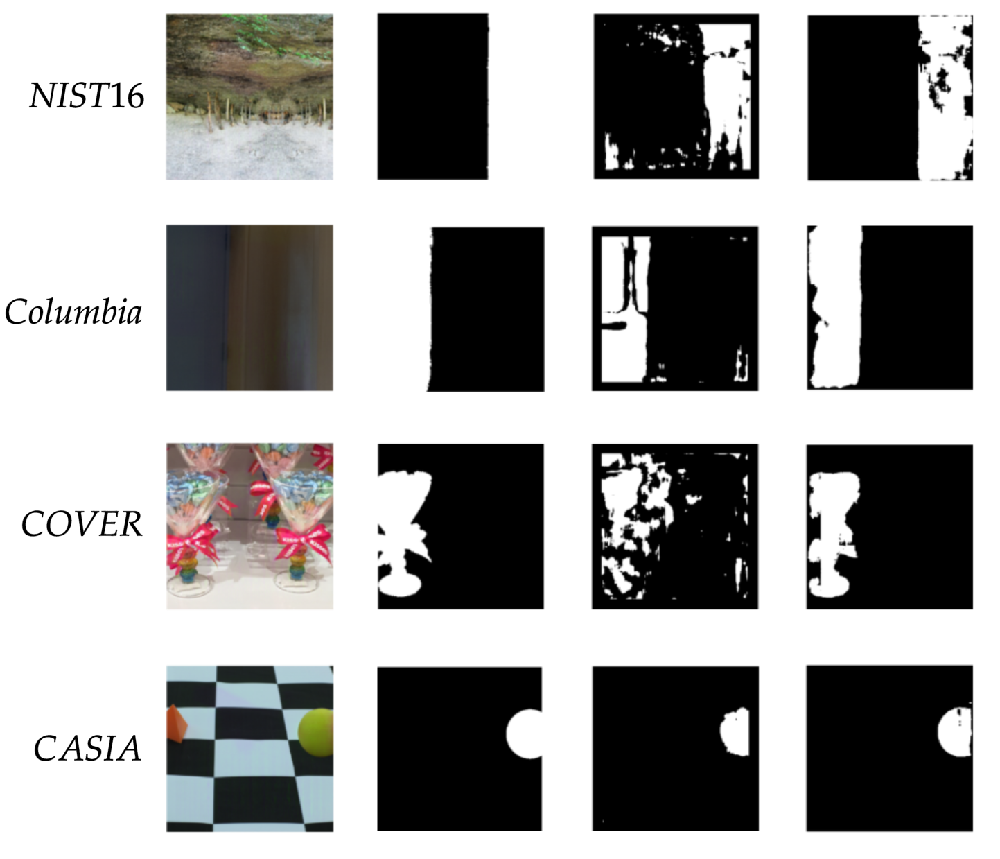
Figure 5: Some of our splice-detection results using examples (in the (ee) scheme) taken from four existing benchmarks. From left to right: input image, ground truth mask, estimated mask via per-pixel threshold (Ours+L), estimated mask via post-trained splice network (Ours+N).

We evaluate using four existing benchmarks: NIST-16 [1], Columbia [11], COVERAGE [28], and CASIA [7]. Each benchmark includes labeled pairs $(I,{\cal M})$ that we downsample to $400\times 400$. Figure 5 shows examples and Table 1 provides numbers, both with comparisons to previous methods that do not use proactive embedding (i.e., that are “reactive” according to the taxonomy of Section 2). The table uses superscript F to indicate methods that are fine-tuned separately for each dataset; and superscript O to indicate methods that use an optimal, oracle-provided threshold for each image (analogous to $\alpha$ in Eq. 9), which is a common practice for these benchmarks [37, 23, 34].

As expected, our proactive-encoding approach can outperform purely reactive ones. Applying a simple per-pixel threshold after the regression operator (Ours+L) already does better in many cases, and post-training a dedicated splice-detection U-Net $h_{\phi}$ (Ours+N), even with very simple synthetic data, does even better by exploiting the spatial coherence of mask-shapes. We find that it substantially outperforms all existing splice detectors, without fine-tuning and without oracle thresholding. We also find, for all variations of our model, that detection accuracy is similar across the (ee) and (eu) situations.

Table 1: Splice mask $F_{1}$-scores on four benchmarks. Superscript F indicates a method is fine-tuned separately for each benchmark dataset, and superscript O indicates a method uses an optimal, oracle-provided threshold for each image within a dataset. Missing entries are not available in prior literature.

Method	NIST16	Columbia	COVER.	CASIA
FOELA [14]	0.236	0.470	0.222	0.214
FONOI1 [21]	0.285	0.574	0.269	0.263
FOCFA1 [9]	0.174	0.467	0.190	0.207
FOMFCN [23]	0.571	0.612	-	0.541
FORGB-N [37]	0.722	0.697	0.437	0.408
FOSPAN [12]	0.582	-	0.558	0.382
FOOurs + L (eu)	0.535	0.500	0.650	0.390
FOOurs + L (eu)	0.658	0.569	0.706	0.585
FOOurs + N (eu)	0.835	0.800	0.890	0.704
FOOurs + L (ee)	0.526	0.535	0.639	0.388
FOOurs + L (ee)	0.659	0.606	0.719	0.595
FOOurs + N (ee)	0.843	0.809	0.881	0.733

4.4 Robustness to Allowable Distortions

Many sharing practices involve transferring images between devices that have varying communication bandwidths and display resolutions, so it is common—at least when archival quality is not concerned—for images to experience distortions such as tone-adjustment and downsampling. Society often accepts these distortions as “allowable” because they provide convenience without substantially altering the intent of the image creator. It is desirable for a system like ours to be insensitive to as many of these distortions as possible, because it enables a greater number of images to be properly certified as being trustworthy.

The bottom of Figure 6 demonstrates the performance of our splice detector (Ours+N in the (eu) scheme) when increasing levels of i.i.d. zero-mean Gaussian noise are added to the received image $\hat{I}$ before passing it to the decoder. In general we find that even without augmenting our training pipeline, our detection degrades gracefully until noise levels reach $10\%$ or more. As a point of reference, we also show the performance of a recent engineered method for block-level protection [17], which impressively provides the additional capability of reconstructing the masked out-portion of a spliced image from its encoding, but fails to operate effectively even when the pixel values are affected by very small changes.

Figure 6: Robustness to additive noise for the baboon image. Noise increases from right to left. From top to bottom: spliced image with added Gaussian noise; splice detection using block-level protection [17]; and splice detection using our approach.

Additional experiments with other types of distortions are included in the supplement.

4.5 Learned Residuals: Statistics and Structure

Minimizing the loss in Equation (8) forces the encoder and decoder to learn a balance between positional accuracy and perceptual distortion. We can examine what they have learned by analyzing the statistics and structure of the residual images they create and use.

We start with first order statistics: Figure 7(a) shows normalized RGB histograms of the residual values $\gamma(x,y,c)$ created by the encoder for a single representative image that was not in the training set. (The residual histograms that are generated for all other input images are very similar.) The residual histograms are very different from the RGB histograms of the input image (b), and instead are more similar to those of a band-pass filtered version of the input image (c). The mean residual RGB value is $(0.002,0.000,0.004)$, which indicates that the overall color cast that it adds to the image is almost negligible.

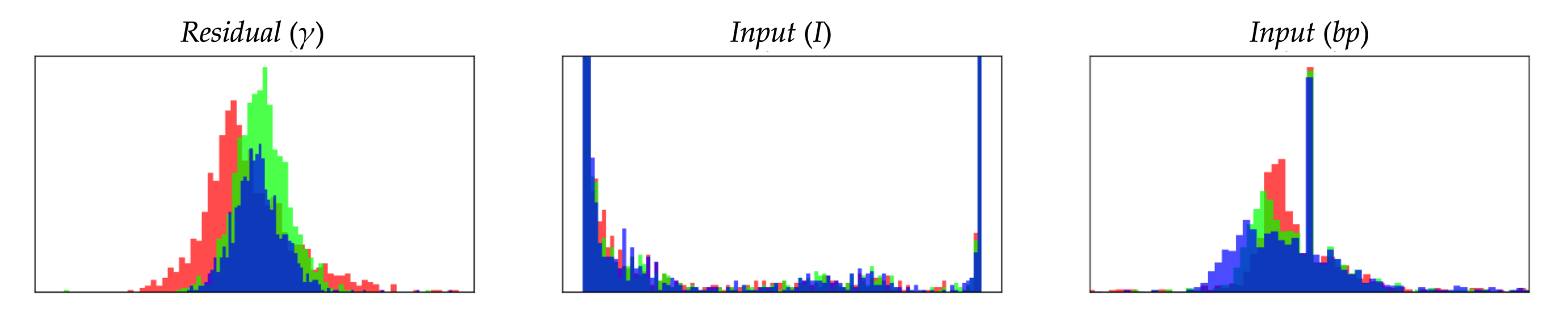
Figure 7: The RGB histogram of a residual image $\gamma$ (left) is different from that of its input image (middle) and is more similar to that of a bandpass-filtered input image (right).

To explore the second-order statistics, we compute the mean residual color $\mu_{\gamma}$, subtract this mean from the per-pixel residual values of a single image, and compute the principal components of the resulting collection of three-vectors $(\gamma(x,y)-\mu_{\gamma})\in\mathbb{R}^{3}$. Surprisingly, we find that $98\%$ of the variance in this set is explained by the first two components, indicating that the distribution of residual colors is highly concentrated near a plane in RGB space. This is in strong contrast to the distribution of colors in the input image, for which only $69\%$ of the variance is explained by the same plane. The “residual plane” is visualized in Figure 8. It comes close to containing the line of greys, and it contains a line of chromaticities spanning from roughly green to purple. This suggests that in the future, it may be worth exploring encoder architectures that create only bi-valued residuals and then combine them via

$$\mu+a_{\theta}(x,y;\begin{bmatrix}I;\Psi\end{bmatrix})v_{1}+b_{\theta}(x,y;\begin{bmatrix}I;\Psi\end{bmatrix})v_{2},$$ (10)

where $\mu,v_{1},v_{2}\in\mathbb{R}^{3}$ are learned in conjunction with network parameters $\theta$. This would reduce encoder computation and could also help stabilize training.

Figure 8: Residual colors $\gamma$ are highly concentrated near a plane in RGB color space. The plane is roughly spanned by the line of greys (in direction $v_{2}$) and by a line of chromaticities from green to purple (in direction $v_{1}$).

5 Conclusion and Societal Impact

Our proof-of-concept model shows that it is possible, using relatively simple CNNs, to steganographically inject localized positional signatures into images, and then to exploit these signatures for detecting crops and replacements in a way that can survive common distortions like tone adjustment and downsampling. This motivates exploring how to scale the approach to practical image sizes. It could help individuals and online platforms to know when an image can be certified as having been published by a trusted pool of content creators, and which parts of such an image, if any, have been substantially altered since publication.

We emphasize that our encoding can only help determine whether an image is faithful to the creator’s intent and does not provide information about the nature of their intention. There is a risk that an authorised creator could abuse our system by intentionally encoding and publishing a fake or misleading image, thereby fooling individuals and platforms into thinking the image can be trusted. Similarly, an adversary could gain access to the encoder and use it to create an encoded image that is later falsely certified as trustworthy and having originated from the authorised pool of creators. Thus, any deployment would need to ensure that the encoder can only be accessed through a secure API, and that only certified, trustworthy agents can access it.

There is also a risk if an adversary gains uncontrolled access to the decoder. It is possible (but much less efficient) to create a stegapos embedding for a particular image without the encoder, by fixing the decoder and back-propagating the loss to the residual. An adversary could use this back-propagation attack as another way to create an image that is falsely trusted.

The risk of such backpropagation attacks could be reduced by requiring clients to query the decoder through a secure API—either to a server or to client-side confidential computing architecture—that prevents the use of differentiation for efficient backpropagation. Risk could be further reduced by limiting the temporal frequency of a client’s queries to the decoder, or by preventing the client from making repeated queries using similar inputs, so that backpropagation with numerical differentiation becomes prohibitive in time.

Finally, we note that it may be possible for an adversary to effectively “erase” the stegapos-encoding from an image by creating and applying a large-but-imperceptible distortion that prevents the decoder from being able to detect any stegapos-encoding. This could preclude clients from being able to certify an image as trustworthy even though it may be a faithful rendition of an authorised creator’s intent. Reducing this risk would require expanding the set of “allowable distortions” that the encoder and decoder are trained against, perhaps using an adversarial approach as proposed for conventional deep watermarking [20].

Acknowledgements. This work is supported by the National Science Foundation under Cooperative Agreement PHY-2019786 (an NSF AI Institute, http://iaifi.org).

References

-
[1]
Nist-16 dataset.
https://www.nist.gov/itl/iad/mig/open-media-forensics-challenge. - [2] Why the way an image is cropped can change everything. The Observers. https://observers.france24.com/en/20180824-verification-guide-cropped-photo-video.
- [3] Mahdi Ahmadi, Alireza Norouzi, Nader Karimi, Shadrokh Samavi, and Ali Emami. ReDMark: Framework for residual diffusion watermarking based on deep networks. Expert Systems with Applications, 146:113157, 2020.
- [4] Shumeet Baluja. Hiding images in plain sight: Deep steganography. In Neural Information Processing Systems, 2017.
- [5] Abdullah Bamatraf, Rosziati Ibrahim, and Mohd. Najib Mohd. Salleh. A new digital watermarking algorithm using combination of least significant bit (lsb) and inverse bit, 2011.
- [6] Mahbuba Begum and Mohammad Shorif Uddin. Digital image watermarking techniques: A review. Information, 11(2), 2020.
- [7] J. Dong, W. Wang, and T. Tan. Casia image tampering detection evaluation database 2010. http://forensics.idealtest.org.
- [8] W. Fan, S. Agarwal, and H. Farid. Rebroadcast attacks: Defenses, reattacks, and redefenses. In 2018 26th European Signal Processing Conference (EUSIPCO), pages 942–946, 2018.
- [9] P. Ferrara, T. Bianchi, A. De Rosa, and A. Piva. Image forgery localization via fine-grained analysis of cfa artifacts. IEEE Transactions on Information Forensics and Security, 7(5):1566–1577, 2012.
- [10] Jamie Hayes and George Danezis. Generating steganographic images via adversarial training. arXiv preprint arXiv:1703.00371, 2017.
- [11] Y.-F. Hsu and S.-F. Chang. Detecting image splicing using geometry invariants and camera characteristics consistency. In International Conference on Multimedia and Expo, 2006.
- [12] Xuefeng Hu, Zhihan Zhang, Zhenye Jiang, Syomantak Chaudhuri, Zhenheng Yang, and Ram Nevatia. Span: Spatial pyramid attention network for image manipulation localization. In Andrea Vedaldi, Horst Bischof, Thomas Brox, and Jan-Michael Frahm, editors, Computer Vision – ECCV 2020, pages 312–328, Cham, 2020. Springer International Publishing.
- [13] David Hume Kennerly. Essay: Chop and crop. The New York Times. https://lens.blogs.nytimes.com/2009/09/17/essay-9/.
- [14] Neal Krawetz and Hacker Factor Solutions. A picture’s worth. Hacker Factor Solutions, 6(2):2, 2007.
- [15] Anders Boesen Lindbo Larsen, Søren Kaae Sønderby, Hugo Larochelle, and Ole Winther. Autoencoding beyond pixels using a learned similarity metric. In International conference on machine learning, 2016.
- [16] Tien-You Lee and Shinfeng D. Lin. Dual watermark for image tamper detection and recovery. Pattern Recognition, 41(11):3497–3506, 2008.
- [17] Yewen Li, Wei Song, Xiaobing Zhao, Juan Wang, and Lizhi Zhao. A Novel Image Tamper Detection and Self-Recovery Algorithm Based on Watermarking and Chaotic System. Mathematics, 7(10):1–17, October 2019.
- [18] Phen Lan Lin, Chung-Kai Hsieh, and Po-Whei Huang. A hierarchical digital watermarking method for image tamper detection and recovery. Pattern Recognition, 38(12):2519–2529, 2005.
- [19] Jonathan Long, Evan Shelhamer, and Trevor Darrell. Fully convolutional networks for semantic segmentation. In Proceedings of the IEEE conference on computer vision and pattern recognition, pages 3431–3440, 2015.
- [20] Xiyang Luo, Ruohan Zhan, Huiwen Chang, Feng Yang, and Peyman Milanfar. Distortion agnostic deep watermarking. In Proceedings of the IEEE/CVF Conference on Computer Vision and Pattern Recognition, 2020.
- [21] Babak Mahdian and Stanislav Saic. Using noise inconsistencies for blind image forensics. Image Vision Comput., 27(10):1497–1503, September 2009.
- [22] Olaf Ronneberger, Philipp Fischer, and Thomas Brox. U-net: Convolutional networks for biomedical image segmentation. In International Conference on Medical image computing and computer-assisted intervention, pages 234–241. Springer, 2015.
- [23] Ronald Salloum, Yuzhuo Ren, and C.-C. Jay Kuo. Image splicing localization using a multi-task fully convolutional network (mfcn). Journal of Visual Communication and Image Representation, 51:201–209, Feb 2018.
- [24] Matthew Tancik, Ben Mildenhall, and Ren Ng. Stegastamp: Invisible hyperlinks in physical photographs. In Proceedings of the IEEE/CVF Conference on Computer Vision and Pattern Recognition, pages 2117–2126, 2020.
- [25] W. Tang, S. Tan, B. Li, and J. Huang. Automatic steganographic distortion learning using a generative adversarial network. IEEE Signal Processing Letters, 24(10):1547–1551, 2017.
- [26] Basile Van Hoorick and Carl Vondrick. Dissecting image crops. arXiv preprint arXiv:2011.11831, 2020.
- [27] Ashish Vaswani, Noam Shazeer, Niki Parmar, Jakob Uszkoreit, Llion Jones, Aidan N Gomez, Lukasz Kaiser, and Illia Polosukhin. Attention is all you need. arXiv preprint arXiv:1706.03762, 2017.
- [28] B. Wen, Y. Zhu, R. Subramanian, T. Ng, X. Shen, and S. Winkler. Coverage — a novel database for copy-move forgery detection. In 2016 IEEE International Conference on Image Processing (ICIP), pages 161–165, 2016.
- [29] Eric Wengrowski and Kristin Dana. Light field messaging with deep photographic steganography. In Proceedings of the IEEE/CVF Conference on Computer Vision and Pattern Recognition (CVPR), June 2019.
- [30] Eric Wengrowski and Kristin Dana. Light field messaging with deep photographic steganography. In 2019 IEEE/CVF Conference on Computer Vision and Pattern Recognition (CVPR), pages 1515–1524, 2019.
- [31] Pin Wu, Yang Yang, and Xiaoqiang Li. Stegnet: Mega image steganography capacity with deep convolutional network. Future Internet, 10(6):54, Jun 2018.
- [32] Y. Wu, W. AbdAlmageed, and P. Natarajan. Mantra-net: Manipulation tracing network for detection and localization of image forgeries with anomalous features. In 2019 IEEE/CVF Conference on Computer Vision and Pattern Recognition (CVPR), pages 9535–9544, 2019.
- [33] Ido Yerushalmy and Hagit Hel-Or. Digital image forgery detection based on lens and sensor aberration. International Journal of Computer Vision, 92(1):71–91, 2011.
- [34] Markos Zampoglou, Symeon Papadopoulos, and Yiannis Kompatsiaris. Large-scale evaluation of splicing localization algorithms for web images. Multimedia Tools Appl., 76(4):4801–4834, February 2017.
- [35] Kevin Alex Zhang, Alfredo Cuesta-Infante, Lei Xu, and Kalyan Veeramachaneni. Steganogan: High capacity image steganography with gans. arXiv preprint arXiv:1901.03892, 2019.
- [36] Richard Zhang, Phillip Isola, Alexei A. Efros, Eli Shechtman, and Oliver Wang. The unreasonable effectiveness of deep features as a perceptual metric. CoRR, abs/1801.03924, 2018.
- [37] Peng Zhou, Xintong Han, Vlad I Morariu, and Larry S Davis. Learning rich features for image manipulation detection. In Proceedings of the IEEE Conference on Computer Vision and Pattern Recognition, pages 1053–1061, 2018.
- [38] Jiren Zhu, Russell Kaplan, Justin Johnson, and Li Fei-Fei. Hidden: Hiding data with deep networks. In Proceedings of the European conference on computer vision (ECCV), pages 657–672, 2018.