Causal Learning for Socially Responsible AI

Abstract

There have been increasing concerns about Artificial Intelligence (AI) due to its unfathomable potential power. To make AI address ethical challenges and shun undesirable outcomes, researchers proposed to develop socially responsible AI (SRAI). One of these approaches is causal learning (CL). We survey state-of-the-art methods of CL for SRAI. We begin by examining the seven CL tools to enhance the social responsibility of AI, then review how existing works have succeeded using these tools to tackle issues in developing SRAI such as fairness. The goal of this survey is to bring forefront the potentials and promises of CL for SRAI.

1 Introduction

Artificial Intelligence (AI) comes with both promises and perils. AI significantly improves countless aspects of day-to-day life by performing human-like tasks with high efficiency and precision. It also brings potential risks for oppression and calamity because how AI works has not been fully understood and regulations surround its use are still lacking Cheng et al. (2021). Many striking stories in media (e.g., Stanford’s COVID-19 vaccine distribution algorithm) have brought Socially Responsible AI (SRAI) into the spotlight.

Substantial risks can arise when AI systems are trained to improve accuracy without knowing the underlying data generating process (DGP). First, the societal patterns hidden in the data are inevitably injected into AI algorithms. The resulting socially indifferent behaviors of AI can be further exacerbated by data heterogeneity and sparsity. Second, lacking knowledge of the DGP can cause researchers and practitioners to unconsciously make some frame of reference commitment to the formalization of AI algorithms Getoor (2019); Cheng et al. (2021), spanning from data and label formalization to the formalization of evaluation metrics. Third, DGP is also central to identifying the cause-effect connections and the causal relations between variables, which are two indispensable ingredients to achieve SRAI. We gain in-depth understanding of AI by intervening, interrogating, altering its environment, and finally answering “what-if” questions.

Causal inference is the key to uncovering the real-world DGPs Pearl (2009). In the era of big data, especially, it is possible to learn causality by leveraging both causal knowledge and the copious real-world data, i.e., causal learning (CL) Guo et al. (2020a). There have been growing interests seeking to improve AI’s social responsibility from a CL perspective, e.g., causal interpretability Moraffah et al. (2020) and causal-based machine learning fairness Makhlouf et al. (2020). In this survey, therefore, we first examine the seven tools in CL that are inherently related to SRAI. We then review existing efforts of connecting four of these tools to emerging tasks in SRAI, including bias mitigation, fairness, transparency, and generalizability/invariance. We conclude with open problems and challenges of leveraging CL to enhance both the functionality and social responsibility of AI.

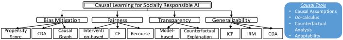
Figure 1: The taxonomy of CL for SRAI. The blue rectangle denotes the four commonly used causal tools for SRAI.

2 Causal Tools for Socially Responsible AI

Based on the available causal information, we can describe CL in a three-layer hierarchy: association, intervention, and counterfactual Pearl (2019). At the first layer, association seeks statistical relations between variables, i.e., $p(y|x)$. By contrast, intervention and counterfactual demand causal information. An intervention is a change to the DGP. With $do$-calculus Pearl (2009), the interventional distribution $p(y|do(x))$ describes the distribution of $Y$ if we force $X$ to take the value $x$ while keeping the rest in the process same. This corresponds to removing all the inbound arrows to $X$ in the causal graph. At the top layer is counterfactual, denoted as $p(y_{x}|x^{\prime},y^{\prime})$. It stands for the probability of $Y=y$ had $X$ been $x$ given what we observed were $X=x^{\prime}$ and $Y=y^{\prime}$.

In the rest of this section, we review the seven tools of CL introduced in Pearl (2019) and briefly discuss how it naturally steers a course towards a SRAI-future.

• Causal Assumptions make an AI system more transparent and testable. Encoding causal assumptions explicitly allows us to discern whether these assumptions are plausible and compatible with available data. It also improves our understandings of how the system works and gives a precise framework to debate Cloudera (2020).

• Do-calculus enables the system to exclude spurious correlations by eliminating confounding through back-door criterion Pearl (2009). Confounding is a major cause of many socially indifferent behaviors of an AI system.

• Counterfactual analysis involves a “what would have happened if” question. It is the building block of scientific thinking, thus, a key ingredient to warrant SRAI.

• Mediation Analysis decomposes the effect of an intervention into direct and indirect effects. Its identification helps understand how and why a cause-effect arises. Therefore, mediation analysis is essential for generating explanations.

• Adaptability is a model’s capability to generalize to different environments. AI algorithms typically cannot perform well when the environment changes. CL can uniquely identify the underlying mechanism responsible for the changes.

• Missing data is a common problem in AI tasks. It reduces statistical power, data representativeness, and can cause biased estimations. CL can help recover causal and statistical relationships from incomplete data via causal graphs.

• Causal discovery learns causal directionality between variables from observational data. As causal graphs are mostly unknown and arbitrarily complex in real-world applications, causal discovery offers a ladder to true causal graphs.

We propose the taxonomy of CL for SRAI in Fig. 1 and review how these CL tools – particularly, the Causal Assumptions, Do-calculus, Counterfactual Analysis, and Adaptability – help SRAI in terms of bias mitigation, fairness, transparency, and generalizability/invariance below.

3 Bias Mitigation

AI systems can be biased due to hidden or neglected biases in the data, algorithms, and user interaction. Olteanu et al. (2019) introduced 23 different types of bias including selection, measurement biases, and so on. There are various ways to de-bias AI systems such as adversarial training Zhang et al. (2018), reinforcement learning Wang and Deng (2020), and causal inference Zhao et al. (2019). Due to its interpretable nature, causal inference offers high confidence in making decisions and can show the relation between data attributes and AI system’s outcomes. Here, we review two popular causality-based methods for bias mitigation – propensity score and counterfactual data augmentation (CDA).

3.1 Propensity Score

Propensity score is used to eliminate treatment selection bias and ensure the treatment and control groups are comparable. It is the “conditional probability of assignment to a particular treatment given a vector of observed covariates” Rosenbaum and Rubin (1983). Due to its effectiveness and simplicity, propensity score has been used to reduce unobserved biases in various domains, e.g., NLP and recommender systems. Here, we focus our discussions on recommender systems.

Inverse Propensity Scoring (IPS) is used to alleviate the selection and position biases commonly present in recommender systems. Selection bias appears when users selectively rate or click items, rendering observed ratings not representative of the true ratings, i.e., ratings obtained when users randomly rate items. Given a user-item pair $(u,i)$ and $O_{u,i}\{0,1\}$ denoting whether $u$ observed $i$, we define propensity score as $P_{u,i}=P(O_{u,i}=1)$, i.e., the marginal probability of observing a rating. During the model training phase, IPS-based unbiased estimator is defined using following empirical risk function Schnabel et al. (2016):

$$\small\operatorname*{arg\,min}_{\theta}\sum_{O_{u,i}=1}\frac{\hat{\sigma}_{u,i}(r,\hat{r}(\theta))}{P_{u,i}}+Reg(\theta),$$ (1)

where $\hat{\sigma}_{u,i}(r,\hat{r}(\theta))$ denotes an evaluation function and $Reg(\theta)$ the regularization for model complexity. IPS is also used to mitigate selection bias during evaluation, see, e.g., Schnabel et al. (2016); Yang et al. (2018).

Position bias occurs in a ranking system as users tend to interact with items with higher ranking positions. To remedy position bias, previous methods used IPS to weigh each data instance with a position-aware value. The loss function of such models is defined as follows Agarwal et al. (2019): $L(M,q)=\sum_{x\in\pi_{q}}\Delta(x,y|\pi_{q}),$ where $M$ indicates the ranking model, $q\in Q$ denotes a query from a set of all queries to the model, $\pi_{q}$ is the ranked list by $M$, and $\Delta(x,y|\pi_{q})$ denotes the individual loss on each item $x$ with relevant label $y$. In another method, Hofmann et al. (2013) proposed to estimate propensity scores using ranking randomization. First, the ranking results of the system are randomized. Then the propensity score is calculated based on user clicks on different positions. Although this method is shown to be effective, it can significantly degrade user experience as the highly ranked items may not be users’ favorites Joachims et al. (2017). Therefore, Guo et al. (2020b) proposed a method in an offline setting where randomized experiments are not available. They specifically considered multiple types of user feedback and applied IPS to learn an unbiased ranking model.

3.2 Counterfactual Data Augmentation (CDA)

CDA is a technique to augment training data with their counterfactually-revised counterparts via causal interventions that seek to eliminate spurious correlations Kaushik et al. (2020). It enables AI algorithms to be trained on unseen data, therefore, reducing undesired biases and improving model generalizability. Here, we focus on CDA for bias mitigation and will discuss model generalizability in Sec. 6.3.

One of the domains using CDA to reduce biases hidden in the data is NLP. Particularly, one begins by sampling a subset of original data that contains attributes of interest, e.g., gender or sentiment. Then expert annotators or inference models are asked to generate the counterfactual counterparts. The augmented datasets are later fed into the downstream NLP tasks, e.g., sentiment analysis. For example, CDA can be used to reduce gender bias by generating a dataset that encourages training algorithms not to capture gender-related information. One such method generates a gender-free list of sentences using a series of sentence templates to replace every occurrence of gendered word pairs (e.g., he:she, her:him/his) Lu et al. (2020b). It formally defined CDA as:

Definition 1

Given input instances $S=\{(x_{1},y_{1}),(x_{2},y_{2}),...,$ $(x_{N},y_{N})\}$ and intervention $c$, a $c$-augmented dataset $S^{\prime}$ is $S\cup\{(c(x),y)\}_{(x,y)\in S}$.

The underlying assumption is that an unbiased model should not distinguish between matched pairs and should produce the same outcome for different genders Lu et al. (2020b). For sentiment analysis, Kaushik et al. (2020) generated counterfactual scenarios with help of human annotators who were provided with positive movie reviews and were asked to perform minimal changes to make them negative.

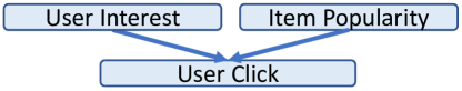
Figure 2: A causal graph to mitigate popularity bias.

3.3 Causal Graphs

Causal graph is a powerful approach for counterfactual reasoning as it allows us to study the effects of various sensitive attributes on the outcome. It is a probabilistic graphical model to encode assumptions and widely used to detect and mitigate bias in AI systems. In the NLP domain, for example, to mitigate gender bias in word embeddings, a recent work by Yang and Feng (2020) proposed a causal graph characterizing relation between gender-definition and gender-biased non-gender-definition word vectors. In the domain of recommender systems, causal graph can mitigate bias that affects decisions toward popular items (i.e., popularity bias) or gender-specific recommendations. The underlying assumption is that, a user click on biased recommendation results from two independent causes: user interest and item popularity. Or formally, $P_{\text{click}}=P_{\text{user interest}}+P_{\text{item popularity}},$ where $P$ indicates matching probability for a user and an item. A corresponding causal graph that disentangles user interest and item popularity is shown in Fig. 2. They further created two different embeddings to capture users’ real-interest in items and pseudo-interest caused by popularity. Finally, the user interest embedding is used to create a de-biased recommender where the popularity bias has been disentangled.

3.4 Discussions

Bias is a primary reason that AI systems fail to make fair decisions. Using propensity-score-based approaches needs to specify the correct forms of propensity scores in real-world applications. The alternate randomization experiments – which may be inapplicable due to ethical and financial considerations – might decrease the utility performance of the AI systems Joachims et al. (2017). One challenge of using CDA is to design a process to generate a modified dataset using the considered interventions. While causal graphs appear promising Yang and Feng (2020), one has to make assumptions that may be impractical to reflect real-world biases. Beyond bias mitigation, measuring bias via experimentation can help understand causal connections between attributes of interest and algorithmic performance Balakrishnan et al. (2020), therefore, mitigating biases.

4 Fairness

Biases in AI systems can lead to many undesired consequences such as model overfitting and other societal issues. One of the most frequently discussed issues in AI is fairness, the property of a model that produces results independent of given variables, especially those considered sensitive, e.g., gender. Here, we briefly review another line of research that aims to train a fair AI system apart from the de-biasing perspective discussed above. A comprehensive survey on causal fairness can be referred to Makhlouf et al. (2020).

4.1 Fairness via Causal Modeling

From the causal perspective, fairness can be formulated as estimating causal effects of sensitive attributes such as gender on the outcome of an AI system. Such causal effects are evaluated using counterfactual interventions over a causal graph with features, sensitive attributes, and other variables. Underpinning this approach is the concept of counterfactual fairness (CF) Kusner et al. (2017). CF implies that a decision is considered fair if it is the same in both “the actual world” and “a counterfactual world” where, e.g., for an individual belongs to a different demographic group. Formally, considering $Y$, $A$, and $X$ as the observed outcome, sensitive attributes, and features, respectively, CF is defined as follows:

Definition 2

Given $x\in X$ and $a\in A$, predictor $\hat{Y}$ is counterfactually fair if

$$P(\hat{Y}_{A\leftarrow a}(U)=y|X=x,A=a)$$ (2)

$$=P(\hat{Y}_{A\leftarrow a^{\prime}}(U)=y|X=x,A=a)$$

holds for all $y$ and any $a^{\prime}\in A$.

$U$ refers to a set of latent background variables in a causal graph. This definition states that if the two outcome probabilities $P(y_{a}|x,a)$ and $P(y_{a^{\prime}}|x,a)$ are equal for an individual, then s/he is treated fairly as if s/he had been from another sensitive group. Or, $A$ should not be the cause of $\hat{Y}$. CF assumed that fairness can be uniquely quantified from observational data, which is not valid in certain situations due to the unidentifiability of the counterfactual quantity. Wu et al. (2019) then introduced a graphical criterion determining the identifiability of counterfactual quantities. With the derived bounds, CF is achieved by constraining the classifier’s training process on the amount of unfairness in the predictor.

Another stepping stone toward creating fair AI systems using CL is the intervention-based fairness. Hajian and Domingo-Ferrer (2012) first proposed to improve fairness by expressing direct and indirect discrimination through the different paths connecting the sensitive attributes (i.e., the treatment) and the outcome of an AI system. Similarly, Zhang and Bareinboim (2018) modeled discrimination based on the effect of a sensitive attribute on an outcome along certain disallowed causal paths. These methods generally formulate and quantify fairness as the average causal effect of the sensitive attribute on the decision attribute, which is then evaluated by the intervention through the post-interventional distributions.

4.2 Discussions

CF considers more general situations than intervention-based fairness where the set of profile attributes is empty, therefore, it is more challenging. One limitation of CF is that these sensitive attributes may not admit counterfactual manipulation Kasirzadeh and Smart (2021). What does it mean to suppose a different version of an individual with the counterfactually manipulated sensitive attributes such as race? In order to use a sensitive attribute appropriately, it is necessary to specify what the categories are and what perception of an attribute to be used. The validity of counterfactuals is also challenging to assess. What is the metric used to measure the similarity between the actual and imaginary worlds? CF-based models may fail when the identifiable assumption is violated due to the unidentifiable counterfactual quantity Wu et al. (2019). Although this might be solved via a relaxed assumption, the idea of using social categories to achieve fairness can be problematic as they may not admit counterfactual manipulation. Lastly, parallel to algorithmic fairness, algorithmic recourse offers explanations and recommendations to individuals unfavourably treated. Future research can consider causal algorithmic recourse and its relation to CF and other fairness criteria von Kügelgen et al. (2020).

5 Transparency

Conventional AI algorithms often lack transparency, typically presented in the concept of interpretability/explanability. When AI algorithms do not provide explanations for how and why they make a decision, users’ trust on these algorithms can be eroded. Hence, there is a need for AI systems to produce interpretable results. Causal Interpretability helps generate human friendly explanations by answering questions such as “Why does a model makes such decisions?”. In this section, we describe two approaches associated with causal interventional interpretability and counterfactual interpretability, respectively. Please refer to Moraffah et al. (2020) for more details.

5.1 Model-based Interpretations

CL for model-based interpretations seeks to estimate the causal effect of a particular input neuron on a certain output neuron in the network. Drawing from causal inference theories, causally interpretable models first map a neural network structure into a Structural Causal Model (SCM) Pearl (2009) and then estimate the effect of each model component on the output based on the data and a learned function (i.e., a neural network) using $do$-calculus Chattopadhyay et al. (2019). Particularly, every $l$-layer neural network $N(l_{1},l_{2},...,l_{n})$ has a corresponding SCM $M([l_{1},...,l_{n}],U,[f_{1},...,f_{n}],P_{U})$ where $f_{i}$ refers to the set of causal functions for neurons in layer $l_{i}$. $U$ denotes a group of exogenous random variables that act as causal factors for input layer $l_{1}$. $P_{u}$ defines the probability distribution of $U$. $M$ can be further reduced to a SCM with only input layer $l_{1}$ and output layer $l_{n}$: $M^{\prime}([l_{1},l_{n}],U,f^{\prime},P_{U})$, by marginalizing out the hidden neurons Chattopadhyay et al. (2019). Finally, we can estimate the average causal effect (ACE) of a feature $x_{i}\in l_{1}$ with value $\alpha$ on output $y\in l_{n}$ by

$$ACE_{do\left(x_{i}=\alpha\right)}^{y}=\mathbb{E}\left[y\mid do\left(x_{i}=\alpha\right)\right]-baseline_{x_{i}},$$ (3)

where $baseline_{x_{i}}=\mathbb{E}_{x_{i}}\left[\mathbb{E}_{y}\left[y\mid do\left(x_{i}=\right.\right.\right.\alpha)]]$.

Similar method was applied to CNN architectures trained on image data to reason over deep learning models Narendra et al. (2018). Zhao and Hastie (2021) leveraged partial dependence plot Friedman (2001) and Individual Conditional Expectation Goldstein et al. (2015) to extract causal information (e.g., relations between input and output variables) from black-box models. Martínez and Marca (2019) proposed an approach for explaining the predictions of a visual model with the causal relations between the latent factors which they leveraged to build a Counterfactual Image Generator.

5.2 Counterfactual Explanations

Different from model-based interpretation which deals with model parameters to determine the vital components of the model, counterfactual explanations typically describe scenarios such as “If X had not occurred, Y would not have occurred”. Specifically, the predicted outcome is considered as the event $Y$ and the features fed to the model are the causes $X$. A counterfactual explanation can be defined as a causal situation of the form where an output $Y$, which occurs given the feature input $X$, can be changed to a predefined output $Y^{\prime}$ by minimally changing the feature vector $X$ to $X^{\prime}$.

To generate counterfactual explanations, a common approach is a generative counterfactual framework Liu et al. (2019) that leverages generative models along with attribute editing mechanisms. The objective function is defined as

$$\small\begin{array}[]{l}\underset{x_{cf}}{\arg\min}\max_{\lambda}L\left(x,x_{cf},y,y_{cf}\right)\\ L\left(x,x_{cf},y,y_{cf}\right)=\lambda\cdot\left(\hat{f}\left(x_{cf}\right)-y_{cf}\right)^{2}+d\left(x,x_{cf}\right),\end{array}$$ (4)

where $x$/$x_{cf}$ denotes the observed/counterfactual features and $y$/$y_{cf}$ the observed/counterfactual outcome. The first term indicates the distance between the model’s prediction for the counterfactual input $x_{cf}$ and the desired counterfactual output. The second term describes the distance between the observed features $x$ and counterfactual features $x_{cf}$. $\lambda$ is the hyperparameter balancing the importance of the two distances. Another category of approach relies on adversarial examples to provide counterfactual explanations. Rather than explaining why a model predicts an output with a given input, it finds an alternative version of the input that receives different classification results. One can also lay constraints on the features so that only the desired features are subject to changes. The third category of approach uses class prototypes for the counterfactual search process Van Looveren and Klaise (2019). These prototypes – refer to the mean encoding of the instances that belong to the class – are integrated into the objective function so that the perturbations can produce interpretable counterfactuals. For a more detailed understanding readers could refer to Xu et al. (2020).

5.3 Discussions

There are still limitations in existing models for causal interepretability. For instance, evaluating such models is difficult due to the lack of ground-truth causal relations between the components of the model or causal effect of one component on another. While using counterfactual explanations for interpretability may seem feasible, it has been shown that there exist unspecified contextual presumptions and choices while generating counterfactual scenarios that may not stand well in the social world Kasirzadeh and Smart (2021). For instance, social categories such as race and gender need to be first defined in order to generate counterfactual scenarios around these variables. Even with ground truth and well-defined social categories, existing works may still fail because causal assumptions in these works are not explicitly explained. It is critical to clearly define causal assumptions.

6 Invariance/Generalizability

Due to societal biases hidden in data and the shortcut learning Geirhos et al. (2020), AI algorithms can easily overfit to training data, i.e., learning spurious correlations. Common approaches for avoiding overfitting rely on the assumption that samples of the entire population are i.i.d., which is rarely satisfied in practice. Violating the i.i.d. assumption leads to poor generalizability of an AI algorithm. Because whether a training and a testing DGP (or environment) differ is unknown, we have recourse to data heterogeneity and a model that is robust to distributional shifts among heterogeneous environments, or the invariance property Arjovsky et al. (2019). Causal relations are, by their nature, invariant Pearl and Bareinboim (2011). Environment is defined by intervention, therefore, in a causal graph, only direct causal relations remain invariant when an intervention changes the environment. We first examine two popular approaches that incorporate the invariance property into predictions.

6.1 Invariant Causal Prediction (ICP)

Built upon SCM, ICP Peters et al. (2016) aims to discover the causal parents (direct causes) of a given variable directly pointing to the target variable without constructing the entire causal graph. We consider the setting where multiple environments $e\in\mathcal{E}$ exist and in each environment $e$, there is a predictor variable $X^{e}\in\mathbb{R}^{p}$ and a target variable $Y^{e}\in\mathbb{R}$. Given a set $S\subseteq\{1,...,p\}$, a vector $X_{S}$ containing all variables $X_{k},k\in S$, ICP assumes Invariant Prediction:

Assumption 1 (Invariant Prediction.)

There is a vector of coefficients $\gamma^{*}=(\gamma_{1}^{*},...,\gamma_{p}^{*})^{\intercal}$ with support $S^{*}:=\{k:\gamma_{k}^{*}\neq 0\}\subseteq\{1,...,p\}$ such that for all $e\in\mathcal{E}$ and $X^{e}$ with an arbitrary distribution:

$$\small Y^{e}=\mu+X^{e}\gamma^{*}+\epsilon^{e},\quad\epsilon^{e}\sim F_{\epsilon},\epsilon^{e}\rotatebox[origin={c}]{90.0}{$\models$}X_{S^{*}}^{e},$$ (5)

where $\mu$ is the intercept and $\epsilon^{e}$ denotes the random noise with the same distribution $F_{\epsilon}$ across all $e\in\mathcal{E}$.

With multiple environments, ICP then fits a linear (Gaussian) regression in each environment. The goal is to find a set of features that results in invariant predictions between environments. In particular, ICP iterates over subsets of features combinatorially and looks for features in a model that are invariant across environments, i.e., invariant coefficients or residuals. The intersection of these sets of features is then a subset of the true direct causes. ICP also relies on the unconfoundedness assumption Pearl (2009): no unobserved confounders exist between input features and the target. In practice, it is common to choose an observed variable to be the environment variable (e.g., background color of an image), when it could plausibly be so. Limited to using linear models and discrete variable for environment separation, Heinze-Deml et al. (2018) extended ICP to a non-linear setting.

6.2 Invariant Risk Minimization (IRM)

Causal graphs are, in many cases, inaccessible, e.g., the causal relations between pixels and a target predict. Without the need to retrieve direct causes of a target variable in a causal graph, IRM Arjovsky et al. (2019) elevates invariance by focusing on out-of-distribution (OOD) generalization – the performance of a predictive model when evaluated in a new environment. IRM seeks to learn a data representation $\phi$ that achieves two goals: predicting accurately and eliciting an invariant predictor across environments. This can be formulated as the constrained optimization problem:

$$\small\min_{\phi:\mathcal{X}\rightarrow\mathcal{Y}}\sum_{e\in\mathcal{E}}R^{e}(\phi)+\lambda\cdot\|\bigtriangledown_{w|w=1.0}R^{e}(w\cdot\phi)\|^{2},$$ (6)

where $\phi$ is the invariant predictor in a latent causal system generating observed features, $w=1.0$ is a fixed “dummy” classifier. $R^{e}(\cdot)$ denotes the risk under $e$ such as prediction errors. $\lambda$ controls the balance between prediction accuracy in each $e$ and the invariance of the predictor $1\cdot\phi(x)$. In practice, the prediction performance in the defined environments is almost certainly reduced due to the exclusion of some spurious correlations. IRM cannot guarantee to remove all spurious correlations as it also depends on the provided environments. There are a number of follow-up works such as Jin et al. (2020); Krueger et al. (2020) relying on a stronger assumption of invariance of $p(y|\phi(x))$ than that of $\mathbb{E}[y|\phi(x)]$ in IRM.

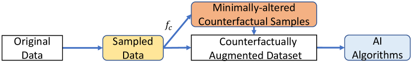
Figure 3: CDA for Invariance. $f_{c}$ is a counterfactual distribution.

6.3 CDA for Invariance/Generalizability

Another causality-inspired approach for improving model invariance is to augment original data with counterfactuals that can expose the model to OOD scenarios. CDA prevents models from learning spurious patterns present in the training data, thus, improving model invariance. A general pipeline describing CDA for model invariance can be seen in Fig. 3.

In computer vision, CDA is used to generate counterfactual images close to training samples yet may not belong to existing training categories. For example, to detect unknown classes, generative adversarial networks were used to generate perturbed examples from the known class and labeled as unknown categories Neal et al. (2018). Drawing on independent mechanisms (IMs) Peters et al. (2017), Sauer and Geiger (2021) proposed to decompose the image generation process into different mechanisms related to its shape, texture, and background. With known causal structure and learned IMs, a counterfactual generative network generated counterfactual images regarding each mechanism. Similar concept was used in visual question answering Abbasnejad et al. (2020) to improve the generalizability of various multimodal and unimodal vision and language tasks.

Inherently related to causal inference, Reinforcement Learning (RL) uses CDA to learn more generalizable policies. Counterfactual data in RL introduces various scenarios that an RL agent generally does not experience during training. In dynamic processes, for instance, Pitis et al. (2020) proposed to decompose the dynamics of different subprocesses into local IMs which can be used to generate counterfactual experiences. To choose the optimal treatment for a given patient, Lu et al. (2020a) proposed a data-efficient RL algorithm that used SCM to generate counterfactual-based data.

6.4 Discussions

Current applications of IRM have been focused on computer vision, nevertheless, an environment needs not to be scenery in an image. Some promising applications include health care Kouw and Loog (2018), robotics Giusti et al. (2015), NLP Choe et al. (2020), recommender systems Wang et al. (2018), and so on. IRM also highly relates to fairness Arjovsky et al. (2019). When applying IRM, one may pay attention to the non-linear settings where formal results for latent-variable models are lacking and risks are under-explored Rosenfeld et al. (2020). Another caveat of existing works in invariant prediction is the reliance on the stringent unconfoundedness assumption, which is typically impractical. ICP is more interpretable than IRM in terms of discovering causal features. For CDA, the counterfactual samples generation strategy usually relieves the conditional independence assumption of training data, which helps improve model generalizability. When generating counterfactual data is not feasible, one can use minimally-different examples in existing datasets with different labels to improve model generalizability Teney et al. (2020).

7 Summary and Open Problems

We review recent advances in SRAI from CL perspective. Purely reliant on statistical relationships, current AI algorithms achieve prominent performance meanwhile its potential risks raise great concerns. To achieve SRAI, we argue that CL is an effective means for it seeks to uncover the DGPs. Our survey begins by introducing the seven CL tools and their connections to SRAI. We then discuss how four of these tools are used in developing SRAI. In the following, we briefly describe promising future research directions of SRAI.

Privacy-preserving.

Privacy is a crucial tenet of SRAI. Many research has shown that AI systems can learn and remember users’ private attributes. However, how to use CL to enhance privacy has been barely studied in literature. Similar to de-biasing methods, we can use CL to remove sensitive information and create privacy-preserving data representations.

Making explicit causal assumptions.

Explicitly making assumptions ensures more valid, testable, and transparent causal models. Given causal assumptions might be disputed or uncertain, we need sensitivity analysis to measure the model performance with assumption violations. Critically, assumptions should be made with humility and researchers are responsible to protect against unethical assumptions.

Causal discovery.

While causal discovery has been extensively studied, its connection to SRAI is not well understood. Discovering causal relations helps determine if assumptions are properly made and interventions are correctly applied. Given that causal graph is key to many CL approaches in SRAI, causal discovery is an important future research.

Mediation analysis.

Causal mediation analysis improves model transparency. For example, in CF, sensitive attributes such as gender and race are assumed to solely have direct influence on the classification. Is the effect of race on loan granting mediated by the job type? Similarly, mediation analysis could be used in explainable AI, e.g., neurons directly or indirectly influence algorithmic decisions.

Missing data.

CL is a missing data problem: inferring the potential outcomes of the same units with different treatment assignments. We might apply CL to a more general setting of missing data. For example, graphical model based procedures can be used to provide performance guarantees when data are Missing Not At Random Mohan and Pearl (2021).

Long-term impact.

The majority of works in SRAI overlooks its long-term commitment to be fulfilled. This hinders both the efficiency and efficacy of existing works to achieve SRAI. For instance, static fairness criterion used in bank loan granting may cost credibility scores of the minorities in the long run Liu et al. (2018).

Social good.

Essentially, SRAI is designed to protect, inform users, and prevent/mitigate the harms of AI Cheng et al. (2021). With the burgeoning AI-for-social-good movement, CL is becoming the core component of AI systems to tackle societal issues.

Causal tools and libraries for SRAI.

SRAI research can also benefit from using existing CL libraries such as Causal ML, DoWhy, and Causal Discovery Toolbox. It is possible to integrate CL models for SRAI into these tools.

References

- Abbasnejad et al. [2020] Ehsan Abbasnejad, Damien Teney, Amin Parvaneh, Javen Shi, and Anton van den Hengel. Counterfactual vision and language learning. In CVPR, pages 10044–10054, 2020.
- Agarwal et al. [2019] Aman Agarwal, Kenta Takatsu, Ivan Zaitsev, and Thorsten Joachims. A general framework for counterfactual learning-to-rank. In SIGIR, 2019.
- Arjovsky et al. [2019] Martin Arjovsky, Léon Bottou, Ishaan Gulrajani, and David Lopez-Paz. Invariant risk minimization. arXiv preprint arXiv:1907.02893, 2019.
- Balakrishnan et al. [2020] Guha Balakrishnan, Yuanjun Xiong, Wei Xia, and Pietro Perona. Towards causal benchmarking of bias in face analysis algorithms. In ECCV, pages 547–563. Springer, 2020.
- Chattopadhyay et al. [2019] Aditya Chattopadhyay, Piyushi Manupriya, Anirban Sarkar, and Vineeth N Balasubramanian. Neural network attributions: A causal perspective. In ICML, pages 981–990. PMLR, 2019.
- Cheng et al. [2021] Lu Cheng, Kush R Varshney, and Huan Liu. Socially responsible ai algorithms: Issues, purposes, and challenges. arXiv preprint arXiv:2101.02032, 2021.
- Choe et al. [2020] Yo Joong Choe, Jiyeon Ham, and Kyubyong Park. An empirical study of invariant risk minimization. In ICML UDL, 2020.
- Cloudera [2020] Cloudera. Causality for machine learning. https://ff13.fastforwardlabs.com/, 2020. Accessed: 2021-02-14.
- Friedman [2001] Jerome H Friedman. Greedy function approximation: a gradient boosting machine. Annals of statistics, pages 1189–1232, 2001.
- Geirhos et al. [2020] Robert Geirhos, Jörn-Henrik Jacobsen, Claudio Michaelis, Richard Zemel, Wieland Brendel, Matthias Bethge, and Felix A Wichmann. Shortcut learning in deep neural networks. Nature Machine Intelligence, 2(11):665–673, 2020.
- Getoor [2019] Lise Getoor. Responsible data science. In Big Data, pages 1–1. IEEE, 2019.
- Giusti et al. [2015] Alessandro Giusti, Jérôme Guzzi, Dan C Cireşan, Fang-Lin He, Juan P Rodríguez, Flavio Fontana, Matthias Faessler, Christian Forster, Jürgen Schmidhuber, Gianni Di Caro, et al. A machine learning approach to visual perception of forest trails for mobile robots. IEEE Robotics and Automation Letters, 1(2):661–667, 2015.
- Goldstein et al. [2015] Alex Goldstein, Adam Kapelner, Justin Bleich, and Emil Pitkin. Peeking inside the black box: Visualizing statistical learning with plots of individual conditional expectation. JCGS, 24(1):44–65, 2015.
- Guo et al. [2020a] Ruocheng Guo, Lu Cheng, Jundong Li, P Richard Hahn, and Huan Liu. A survey of learning causality with data: Problems and methods. CSUR, 53(4):1–37, 2020.
- Guo et al. [2020b] Ruocheng Guo, Xiaoting Zhao, Adam Henderson, Liangjie Hong, and Huan Liu. Debiasing grid-based product search in e-commerce. In KDD, 2020.
- Hajian and Domingo-Ferrer [2012] Sara Hajian and Josep Domingo-Ferrer. A methodology for direct and indirect discrimination prevention in data mining. TKDE, 25(7):1445–1459, 2012.
- Heinze-Deml et al. [2018] Christina Heinze-Deml, Jonas Peters, and Nicolai Meinshausen. Invariant causal prediction for nonlinear models. JCI, 6(2), 2018.
- Hofmann et al. [2013] Katja Hofmann, Anne Schuth, Shimon Whiteson, and Maarten De Rijke. Reusing historical interaction data for faster online learning to rank for ir. In WSDM, pages 183–192, 2013.
- Jin et al. [2020] Wengong Jin, Regina Barzilay, and Tommi Jaakkola. Domain extrapolation via regret minimization. arXiv preprint arXiv:2006.03908, 2020.
- Joachims et al. [2017] Thorsten Joachims, Adith Swaminathan, and Tobias Schnabel. Unbiased learning-to-rank with biased feedback. In WSDM, pages 781–789, 2017.
- Kasirzadeh and Smart [2021] Atoosa Kasirzadeh and Andrew Smart. The use and misuse of counterfactuals in ethical machine learning. In FAccT, 2021.
- Kaushik et al. [2020] Divyansh Kaushik, Eduard Hovy, and Zachary C Lipton. Learning the difference that makes a difference with counterfactually-augmented data. ICLR, 2020.
- Kouw and Loog [2018] Wouter M Kouw and Marco Loog. An introduction to domain adaptation and transfer learning. arXiv preprint arXiv:1812.11806, 2018.
- Krueger et al. [2020] David Krueger, Ethan Caballero, Joern-Henrik Jacobsen, Amy Zhang, Jonathan Binas, Remi Le Priol, and Aaron Courville. Out-of-distribution generalization via risk extrapolation (rex). arXiv preprint arXiv:2003.00688, 2020.
- Kusner et al. [2017] Matt J Kusner, Joshua R Loftus, Chris Russell, and Ricardo Silva. Counterfactual fairness. NeurIPS, 2017.
- Liu et al. [2018] Lydia T Liu, Sarah Dean, Esther Rolf, Max Simchowitz, and Moritz Hardt. Delayed impact of fair machine learning. In ICML, pages 3150–3158, 2018.
- Liu et al. [2019] Shusen Liu, Bhavya Kailkhura, Donald Loveland, and Yong Han. Generative counterfactual introspection for explainable deep learning. arXiv preprint arXiv:1907.03077, 2019.
- Lu et al. [2020a] Chaochao Lu, Biwei Huang, Ke Wang, José Miguel Hernández-Lobato, Kun Zhang, and Bernhard Schölkopf. Sample-efficient reinforcement learning via counterfactual-based data augmentation. In NeurIPS Offline RL, 2020.
- Lu et al. [2020b] Kaiji Lu, Piotr Mardziel, Fangjing Wu, Preetam Amancharla, and Anupam Datta. Gender bias in neural natural language processing. In Logic, Language, and Security, pages 189–202. Springer, 2020.
- Makhlouf et al. [2020] Karima Makhlouf, Sami Zhioua, and Catuscia Palamidessi. Survey on causal-based machine learning fairness notions. arXiv preprint arXiv:2010.09553, 2020.
- Martínez and Marca [2019] Álvaro Parafita Martínez and Jordi Vitrià Marca. Explaining visual models by causal attribution. In ICCVW, pages 4167–4175. IEEE, 2019.
- Mohan and Pearl [2021] Karthika Mohan and Judea Pearl. Graphical models for processing missing data. JASA, pages 1–42, 2021.
- Moraffah et al. [2020] Raha Moraffah, Mansooreh Karami, Ruocheng Guo, Adrienne Raglin, and Huan Liu. Causal interpretability for machine learning-problems, methods and evaluation. ACM SIGKDD Explorations Newsletter, 22(1):18–33, 2020.
- Narendra et al. [2018] Tanmayee Narendra, Anush Sankaran, Deepak Vijaykeerthy, and Senthil Mani. Explaining deep learning models using causal inference. arXiv preprint arXiv:1811.04376, 2018.
- Neal et al. [2018] Lawrence Neal, Matthew Olson, Xiaoli Fern, Weng-Keen Wong, and Fuxin Li. Open set learning with counterfactual images. In ECCV, 2018.
- Olteanu et al. [2019] Alexandra Olteanu, Carlos Castillo, Fernando Diaz, and Emre Kıcıman. Social data: Biases, methodological pitfalls, and ethical boundaries. Frontiers in Big Data, 2:13, 2019.
- Pearl and Bareinboim [2011] Judea Pearl and Elias Bareinboim. Transportability of causal and statistical relations: A formal approach. In AAAI, volume 25, 2011.
- Pearl [2009] Judea Pearl. Causality. 2009.
- Pearl [2019] Judea Pearl. The seven tools of causal inference, with reflections on machine learning. Communications of the ACM, 62(3):54–60, 2019.
- Peters et al. [2016] Jonas Peters, Peter Bühlmann, and Nicolai Meinshausen. Causal inference by using invariant prediction: identification and confidence intervals. J R Stat Soc Series B Stat Methodol, pages 947–1012, 2016.
- Peters et al. [2017] Jonas Peters, Dominik Janzing, and Bernhard Schölkopf. Elements of causal inference: foundations and learning algorithms. The MIT Press, 2017.
- Pitis et al. [2020] Silviu Pitis, Elliot Creager, and Animesh Garg. Counterfactual data augmentation using locally factored dynamics. In NeurIPS, 2020.
- Rosenbaum and Rubin [1983] Paul R Rosenbaum and Donald B Rubin. The central role of the propensity score in observational studies for causal effects. Biometrika, 70(1):41–55, 1983.
- Rosenfeld et al. [2020] Elan Rosenfeld, Pradeep Ravikumar, and Andrej Risteski. The risks of invariant risk minimization. arXiv preprint arXiv:2010.05761, 2020.
- Sauer and Geiger [2021] Axel Sauer and Andreas Geiger. Counterfactual generative networks. 2021.
- Schnabel et al. [2016] Tobias Schnabel, Adith Swaminathan, Ashudeep Singh, Navin Chandak, and Thorsten Joachims. Recommendations as treatments: Debiasing learning and evaluation. In ICML, 2016.
- Teney et al. [2020] Damien Teney, Ehsan Abbasnedjad, and Anton van den Hengel. Learning what makes a difference from counterfactual examples and gradient supervision. In ECCV, 2020.
- Van Looveren and Klaise [2019] Arnaud Van Looveren and Janis Klaise. Interpretable counterfactual explanations guided by prototypes. arXiv preprint arXiv:1907.02584, 2019.
- von Kügelgen et al. [2020] Julius von Kügelgen, Umang Bhatt, Amir-Hossein Karimi, Isabel Valera, Adrian Weller, and Bernhard Schölkopf. On the fairness of causal algorithmic recourse. arXiv preprint arXiv:2010.06529, 2020.
- Wang and Deng [2020] Mei Wang and Weihong Deng. Mitigating bias in face recognition using skewness-aware reinforcement learning. In CVPR, pages 9322–9331, 2020.
- Wang et al. [2018] Yixin Wang, Dawen Liang, Laurent Charlin, and David M Blei. The deconfounded recommender: A causal inference approach to recommendation. arXiv preprint arXiv:1808.06581, 2018.
- Wu et al. [2019] Yongkai Wu, Lu Zhang, and Xintao Wu. Counterfactual fairness: Unidentification, bound and algorithm. In IJCAI, 2019.
- Xu et al. [2020] Guandong Xu, Tri Dung Duong, Qian Li, Shaowu Liu, and Xianzhi Wang. Causality learning: A new perspective for interpretable machine learning. arXiv preprint arXiv:2006.16789, 2020.
- Yang and Feng [2020] Zekun Yang and Juan Feng. A causal inference method for reducing gender bias in word embedding relations. In AAAI, pages 9434–9441, 2020.
- Yang et al. [2018] Longqi Yang, Yin Cui, Yuan Xuan, Chenyang Wang, Serge Belongie, and Deborah Estrin. Unbiased offline recommender evaluation for missing-not-at-random implicit feedback. In RecSys, 2018.
- Zhang and Bareinboim [2018] Junzhe Zhang and Elias Bareinboim. Fairness in decision-making—the causal explanation formula. In AAAI, volume 32, 2018.
- Zhang et al. [2018] Brian Hu Zhang, Blake Lemoine, and Margaret Mitchell. Mitigating unwanted biases with adversarial learning. In AIES, pages 335–340, 2018.
- Zhao and Hastie [2021] Qingyuan Zhao and Trevor Hastie. Causal interpretations of black-box models. JBES, 39(1):272–281, 2021.
- Zhao et al. [2019] Jieyu Zhao, Tianlu Wang, Mark Yatskar, Ryan Cotterell, Vicente Ordonez, and Kai-Wei Chang. Gender bias in contextualized word embeddings. In NAACL, 2019.