Time-dependent coherent squeezed states in a nonunitary approach

Abstract

In this work, we have applied the integrals of motion method in a nonunitary approach and so obtained the time-dependent displacement and squeezed parameters of the coherent squeezed states (CSS). On its turn, CSS for one-dimensional systems with general time-dependent quadratic Hamiltonian are constructed. We discuss the properties of these states, in particular, minimization of uncertainty relation and transition probabilities. As an application, we calculate the CSS of an oscillator with a time-dependent frequency and shown that the solution can be obtained from these well-known Mathieu’s equation.

I Introduction

The coherent states (CS) have attracted a renewed interest in recent years. In modern quantum physics, they play a fundamental role due to their useful properties and the intrinsic relationship with the description of quantum systems in a semiclassical scenario. Therefore, as a consequence, have been applied in a wide range of studies extending from the quantum theory of radiation Kla1968 ; Scu1997 , mathematical physics Kla1985 , even quantum computation Nel2000 . There is a well-developed scheme of constructing the CS for systems with quadratic Hamiltonians, see Gla1963 ; Per1986 . In particular, the CS are defined by minimizing uncertainty relations for some physical quantities (e.g., position and momentum), with the same standard deviation for each of these physical quantities. Additionally, the minimum uncertainty found for CS is identical to that calculated from the vacuum state.

On the other hand, the CSS are quantum states for which, given specific pairs of physical quantities, the standard deviation evaluated in one of them is smaller than for a CS, provided that the standard deviation into another quantity is increased. As the outcome, the CSS has been applied to improve optical communications Yue1976 , quantum information Slu1990 , and also are essential for the detectors of gravitational waves Cav1981 ; Ni1987 ; Chu2014 . A scheme of constructing the CSS has been developed through the unitary displacement and squeezing operators, which act on the vacuum state see, e.g., Wal1983 ; Fis1984 ; Sat1985 ; Jan1988 ; Nie2000 . See also Dod2002 ; Dod2003 ; Per2018 and the selected articles there.

The time-dependent quadratic Hamiltonian systems have attracted attention over the years because of their usefulness in describing the dynamics of many phenomena in quantum mechanics, quantum optics, see, e.g., Ber1983 ; Sal1989 ; Dod1989 ; Wol1990 ; Aga1991 and therefore offers many applications in various fields of Physics. In the papers Yue1976 ; Yeo2003 ; Bag2015 , the authors solved the Schrödinger equation with a time-dependent general quadratic Hamiltonian. In particular, using the integral of motion method Dod1972 ; Mal1975 ; Mal1979 , some kinds of CSS were constructed in Bag2015 . In this work, a particular set of CSS are constructed as eigenvectors of the integrals of motion with a corresponding complex eigenvalue.

In another way, the CSS also can be constructed using the nonunitary approach Wun1992 ; Roy1992 . This method consists of introducing a nonunitary exponential operator composed of a part of the displacement and squeezed standard operators, which allows us to introduce the most convenient displacement and squeezing parameters. From this procedure, we propose to use the integral of motion method in a nonunitary approach to constructed time-dependent CSS of a time-dependent general quadratic Hamiltonian and its relation with the time-independent Fock-states. We must emphasize that such a relationship is not clearly established in the unitary approach. In this context, there are potential applications in the study of finite-level systems, which have relation, e.g., to the problem of one- and two-qubit gates Brem2002 , in the semiclassical theory of laser beams Nuss1973 , in optical resonance Alle1975 .

In the present paper, we are interested in investigating the properties of the CSS for a general time-dependent quadratic Hamiltonian. Thus, this work is organized as follows. In Sect. 2, following the integral of motion method, we will construct the integrals of motion for this system. On its turn, this allows us to introduce time-dependent displacement and squeezing parameters of CSS in a nonunitary approach. Then, in Sect. 3, we will obtain the representation for the states in terms of Fock-states and the corresponding transition probability. In Sect. 4, we will discuss semiclassical features and coordinate representation of the constructed CSS. Finally, in Sect. 5, as an application of the general construction, we will consider CSS of the time-dependent harmonic oscillator, whose solution, as we shaw see, corresponds to that obtained from the well-known Mathieu’s problem.

II Integrals of motion

The time-dependent general quantum quadratic Hamiltonian system with one degree of freedom in terms of the annihilation $\hat{a}$ and creation $\hat{a}^{\dagger}$ operators $\left(\left[\hat{a},\hat{a}^{\dagger}\right]=1\right)$ is written as

$$\hat{H}=\frac{1}{2}\hbar\left(\alpha^{\ast}\hat{a}^{2}+\alpha\hat{a}^{\dagger 2}\right)+\hbar\beta\hat{a}^{\dagger}\hat{a}+\hbar\gamma^{\ast}\hat{a}+\hbar\gamma\hat{a}^{\dagger}+\hbar\delta,$$ (1)

where $\alpha$, $\beta$, $\gamma$, and $\delta$ are time-dependent functions and the signs $\dagger$ and $\ast$ denote Hermitian and complex conjugation, respectively. From the hermiticity condition, we have that $\beta$ and $\delta$ must be real functions.

On its turn, the quantum states $\left|\Psi\right\rangle$ which describe the time evolution of the system should satisfy the Schrödinger’s equation

$$\hat{\Lambda}\left|\Psi\right\rangle=0,\text{ \ }$$

$$\hat{\Lambda}=\hat{H}-i\hbar\partial_{t},\text{ \ }\partial_{t}=\frac{\partial}{\partial t},$$ (2)

where $\hat{\Lambda}$ we call of equation operator.

Let us consider a time-dependent operator $\hat{A}=\hat{A}\left(t\right)$:

$$\hat{A}=f\hat{a}+g\hat{a}^{\dagger}+\varphi,$$

$$\left[\hat{A},\hat{A}^{\dagger}\right]=1,\text{ \ }\left|f\right|^{2}-\left|g\right|^{2}=1.$$ (3)

Here $f=f\left(t\right)$, $g=g\left(t\right)$ and $\varphi=\varphi\left(t\right)$ are some complex function of $t$, which will be further chosen so that the operator $\hat{A}$ to be integral of motion of the Eq. (2), and implies that

$$\overset{\cdot}{\hat{A}}=\frac{i}{\hbar}\left[\hat{\Lambda},\hat{A}\right]=0,$$ (4)

where, in this case, dot denotes the total derivative with respect to time $t$.

From (3), one can express the operator $\hat{a}$ in terms of the integrals of motion $\hat{A}$ and $\hat{A}^{\dagger}$,

$$\hat{a}=f^{\ast}\hat{A}-g\hat{A}^{\dagger}+u,\text{ \ }u=g\varphi^{\ast}-f^{\ast}\varphi.$$ (5)

Let us consider the generalized coordinate $x$ on the whole real axis and the canonical momentum $\hat{p}=-i\hbar\partial_{x}$ in terms of the operators $\hat{a}$ and $\hat{a}^{\dagger}$ in the form:

$$\hat{a}=\frac{1}{\sqrt{2}}\left(\frac{\hat{x}}{l}+\frac{il}{\hbar}\hat{p}\right),\text{ \ }\hat{a}^{\dagger}=\frac{1}{\sqrt{2}}\left(\frac{\hat{x}}{l}-\frac{il}{\hbar}\hat{p}\right),$$

$$\hat{x}=l\frac{\hat{a}+\hat{a}^{\dagger}}{\sqrt{2}},\text{ \ }\hat{p}=\frac{\hbar}{l}\frac{\hat{a}-\hat{a}^{\dagger}}{i\sqrt{2}},\text{ \ }\left[\hat{x},\hat{p}\right]=i\hbar,$$ (6)

where $l$-parameter has the dimension of length. In terms of these operators, (1) reads,

$$\hat{H}=\frac{\hat{p}^{2}}{2m}+\frac{k}{2}\hat{x}^{2}+\frac{\Omega}{2}\left(\hat{x}\hat{p}+\hat{p}\hat{x}\right)+F\hat{x}+V\hat{p}+\mathcal{E}.$$ (7)

The time-dependent quantities $m=m\left(t\right)$, $k=k\left(t\right)$, $\Omega=\Omega\left(t\right),$ $F=F\left(t\right)$, $V=V\left(t\right)$ and $\mathcal{E}=\mathcal{E}\left(t\right)$ are related with $\beta$, $\alpha$, $\gamma$ and $\delta$ in the form

$$\frac{1}{m}=\frac{l^{2}}{\hbar}\operatorname{Re}\left(\beta-\alpha\right),\text{ \ }k=\frac{\hbar}{l^{2}}\operatorname{Re}\left(\beta+\alpha\right),\text{ \ }\Omega=\operatorname{Im}\left(\alpha\right),\text{ \ }$$

$$F=\frac{\sqrt{2}\hbar}{l}\operatorname{Re}\left(\gamma\right),\text{ \ }V=\sqrt{2}l\operatorname{Im}\left(\gamma\right),\text{ \ }\mathcal{E}=\hbar\left(\delta-\frac{\beta}{2}\right),$$ (8)

with the following initial conditions $m_{0}=m\left(0\right)$, $k_{0}=k\left(0\right)$, $\Omega_{0}=\Omega\left(0\right)$, $F_{0}=F\left(0\right)$, $V_{0}=V\left(0\right)$ and $\mathcal{E}_{0}=\mathcal{E}\left(0\right)$. Furthermore, it can be interesting to find the inverse relation above, which is given by

$$\beta =\frac{l^{2}}{2\hbar}\left(k+\frac{\hbar^{2}}{l^{4}m}\right),\text{ \ }\alpha=\frac{l^{2}}{2\hbar}\left(k-\frac{\hbar^{2}}{l^{4}m}\right)+i\Omega,\text{ \ }$$

$$\gamma =\frac{l}{\hbar\sqrt{2}}\left(F+\frac{i\hbar}{l^{2}}V\right),\text{ \ }\delta=\frac{1}{\hbar}\mathcal{E}+\frac{l^{2}}{4\hbar}\left(k+\frac{\hbar^{2}}{l^{4}m}\right).$$ (9)

Analyzing the relationships above can interpret the role of each parameter present in the Hamiltonian (1) and its effects on the squeezed and displacement parameters, as will be seen later.

From (5) and (6), we can write $\hat{x}$ and $\hat{p}$ in terms of $\hat{A}$ and $\hat{A}^{\dagger}$ in the form

$$\hat{x} =l\frac{\left(f^{\ast}-g^{\ast}\right)\hat{A}+\left(f-g\right)\hat{A}^{\dagger}}{\sqrt{2}}+\sqrt{2}l\operatorname{Re}u,\text{ \ }$$

$$\hat{p} =\frac{\hbar}{l}\frac{\left(f^{\ast}+g^{\ast}\right)\hat{A}-\left(f+g\right)\hat{A}^{\dagger}}{i\sqrt{2}}+\sqrt{2}\frac{\hbar}{l}\operatorname{Im}u.$$ (10)

II.1 Equations for $f$, $g$, and $\varphi$

Substituting the representations (2) and (3) into (4), we may derive a set of differential equations for the functions $f$, $g$ and $\varphi$,

$$i\dot{f}=\alpha^{\ast}g-\beta f,\text{ \ }i\dot{g}=\beta g-\alpha f,\text{ \ }i\dot{\varphi}=\gamma^{\ast}g-\gamma f.$$ (11)

Taking in account the initial conditions $f_{0}=f\left(0\right)=\left|f_{0}\right|e^{i\theta_{1}}$ and $g_{0}=g\left(0\right)=\left|g_{0}\right|e^{i\theta_{2}}$ we may obtain any nontrivial solution for the functions $f$ and $g$. Then the function $\varphi$ can be found by a simple integration

$$\varphi=i\int_{0}^{t}\left(\gamma f-\gamma^{\ast}g\right)d\tau+\varphi_{0},$$ (12)

where $\varphi_{0}=\varphi\left(0\right)=\left|\varphi_{0}\right|e^{i\varsigma}$ is an arbitrary complex constant.

In order to obtain the solution for the functions $f$ and $g$, one may identify the two first equations in (11) with, for instance, the well-known ones spin equation Bag2005 ,

$$i\dot{\psi}=\left(\mathbf{K}\cdot\boldsymbol{\sigma}\right)\psi,$$

$$\psi=\left(\begin{array}[c]{c}f\\ g\end{array}\right),\text{ \ }\mathbf{K}=-\left(i\operatorname{Im}\alpha,-i\operatorname{Re}\alpha,\beta\right),\text{ \ }\boldsymbol{\sigma}=\left(\sigma_{1},\sigma_{2},\sigma_{3}\right),$$ (15)

where $\boldsymbol{\sigma}$ are the Pauli matrices.

For sake simplicity, if we assume that $\alpha$, $\beta$, and $\gamma$ are time-independent, then we can write:

$$\ddot{f}+\Theta^{2}f=0,\text{ \ }\Theta=\sqrt{\beta^{2}-\left|\alpha\right|^{2}}.$$ (16)

This equation has the form of the simple harmonic oscillator equation with a time-independent frequency $\Theta$. Given the exact solution of (16), one may obtain $g$ through the equation

$$g=\frac{i}{\alpha^{\ast}}\dot{f}+\frac{\beta}{\alpha^{\ast}}f.$$ (17)

Thus, the general solution of these equations is

$$f=f_{0}\cos\left(\Theta t\right)+i\left(\beta f_{0}-\alpha^{\ast}g_{0}\right)\frac{\sin\left(\Theta t\right)}{\Theta},\text{ \ }g=g_{0}\cos\left(\Theta t\right)+i\left(\alpha f_{0}-\beta g_{0}\right)\frac{\sin\left(\Theta t\right)}{\Theta},$$

$$\varphi=i\left(\gamma f_{0}-\gamma^{\ast}g_{0}\right)\frac{\sin\left(\Theta t\right)}{\Theta}+\left[\left(\gamma\beta-\gamma^{\ast}\alpha\right)f_{0}+\left(\gamma^{\ast}\beta-\gamma\alpha^{\ast}\right)g_{0}\right]\frac{\cos\left(\Theta t\right)-1}{\Theta^{2}}+\varphi_{0}.$$ (18)

III Time-dependent CSS

Here, let us introduce a nonunitary exponential operator $\hat{S}$, as seen below

$$\hat{S}=\exp\left(\xi\hat{a}^{\dagger}+\frac{1}{2}\zeta\hat{a}^{\dagger 2}\right),$$ (19)

where the time-dependent quantities $\xi=\xi\left(t\right)$ and $\zeta=\zeta\left(t\right)$ corresponds to displacement and squeezed parameters, respectively, in a nonunitary approach to CSS.

Taking into account that

$$\xi=\frac{\varphi}{f},\text{ \ }\zeta=\frac{g}{f},$$ (20)

and using the Baker–Campbell–Hausdorff theorem

$$e^{A}Be^{-A}=B+\left[A,B\right]+\frac{1}{2}\left[A,\left[A,B\right]\right]+\ldots,$$ (21)

one can express the canonical operator $\hat{a}$ through of the integral of motion $\hat{A}$ as follows

$$\hat{a}=\frac{1}{f}\hat{S}\hat{A}\hat{S}^{-1}.$$ (22)

The application from this relation on the vacuum state $\left|0\right\rangle$, which satisfies the annihilation condition $\hat{a}\left|0\right\rangle=0$, yields:

$$\hat{A}\left|\xi,\zeta\right\rangle=0,\text{ }$$ (21a)

where the most general state is given by

$$\text{\ }\left|\xi,\zeta\right\rangle=\Phi\exp\left(-\xi\hat{a}^{\dagger}-\frac{1}{2}\zeta\hat{a}^{\dagger 2}\right)\left|0\right\rangle.$$ (21b)

From here, we call the states $\left|\xi,\zeta\right\rangle$ of time-dependent CSS. Note that the function $\Phi=\Phi\left(t\right)$ was introduced and will be following be determined in such a way that the states $\left|\xi,\zeta\right\rangle$ satisfies the Schrödinger’s equation (2).

Substituting $\left|\xi,\zeta\right\rangle$ into (2), we obtain the following equation for $\Phi$:

$$\frac{\dot{\Phi}}{\Phi}=\frac{\left\langle\zeta,\xi\left|\hat{a}^{\dagger}\right|\xi,\zeta\right\rangle}{\left\langle\zeta,\xi|\xi,\zeta\right\rangle}\dot{\xi}+\frac{1}{2}\frac{\left\langle\zeta,\xi\left|\hat{a}^{\dagger 2}\right|\xi,\zeta\right\rangle}{\left\langle\zeta,\xi|\xi,\zeta\right\rangle}\dot{\zeta}-\frac{i}{\hbar}\frac{\left\langle\zeta,\xi\left|\hat{H}\right|\xi,\zeta\right\rangle}{\left\langle\zeta,\xi|\xi,\zeta\right\rangle}.$$ (22)

Using the representation (5) and the condition (21a), one can calculate the mean values easily in (22), as seen below

$$\frac{\left\langle\zeta,\xi\left|\hat{a}^{\dagger}\right|\xi,\zeta\right\rangle}{\left\langle\zeta,\xi|\xi,\zeta\right\rangle}=u^{\ast},\text{ \ }\frac{\left\langle\zeta,\xi\left|\hat{a}^{\dagger 2}\right|\xi,\zeta\right\rangle}{\left\langle\zeta,\xi|\xi,\zeta\right\rangle}=u^{\ast 2}-fg^{\ast},$$

$$\frac{\left\langle\zeta,\xi\left|\hat{H}\right|\xi,\zeta\right\rangle}{\left\langle\zeta,\xi|\xi,\zeta\right\rangle}=\hbar\operatorname{Re}\left[2\gamma^{\ast}u+\alpha^{\ast}u^{2}-\alpha fg^{\ast}+\beta\left(\left|g\right|^{2}+\left|u\right|^{2}\right)+\delta\right].$$ (23)

Thus, we can rewrite the $\Phi$ function, and so obtain

$$\Phi=\frac{C}{\sqrt{f}}\exp\left(\frac{g^{\ast}}{f}\frac{\varphi^{2}}{2}-\frac{\left|\varphi\right|^{2}}{2}+i\phi\right),$$

$$\phi=\frac{1}{2}\int_{0}^{t}\left(\beta-2\delta\right)d\tau,$$ (24)

where $C$ is a normalization constant, which one may choose $C=1$ such that $\left\langle\zeta,\xi|\xi,\zeta\right\rangle=1$.

Then, normalized time-dependent CSS that satisfies the Schrödinger’s equation have the form

$$\left|\xi,\zeta\right\rangle=\frac{1}{\sqrt{f}}\exp\left(\frac{g^{\ast}}{f}\frac{\varphi^{2}}{2}-\frac{\left|\varphi\right|^{2}}{2}+i\phi\right)\exp\left(-\xi\hat{a}^{\dagger}-\frac{1}{2}\zeta\hat{a}^{\dagger 2}\right)\left|0\right\rangle.$$ (25)

III.1 CSS in Fock-states representation

The representation of the CSS via Fock-states can be obtained by taking into account the generation function of the Hermite polynomials $H_{n}\left(y\right)$; see the formula (10.13.19) in Ede1953 ,

$$\exp\left(2yz-z^{2}\right)={\displaystyle\sum\limits_{n=0}^{\infty}}\frac{H_{n}\left(y\right)}{n!}z^{n},$$ (26)

by applying it to the exponential operator function in (25),

$$\left|\xi,\zeta\right\rangle=\frac{1}{\sqrt{f}}\exp\left(\frac{g^{\ast}}{f}\frac{\varphi^{2}}{2}-\frac{\left|\varphi\right|^{2}}{2}+i\phi\right){\displaystyle\sum\limits_{n=0}^{\infty}}\left(\frac{g}{2f}\right)^{\frac{n}{2}}H_{n}\left(\frac{\varphi}{\sqrt{2gf}}\right)\frac{\left(-1\right)^{n}}{\sqrt{n!}}\left|n\right\rangle.$$ (27)

Here, it is important to highlight that the expansion of time-dependent CSS on the time-independent Fock-states is obtained directly in the nonunitary approach. On the other hand, following the usual construction of these states through integrals of motion, it is unclear how it is possible to obtain an equivalent expansion, see, e.g., Bag2015 . These states, Eq. (27), allow us to obtain the usual CS and squeezed states (SS) classes, as seen below.

1. The particular case $\varphi=0\Rightarrow\xi=0$ leads to the expression of the time-dependent SS

   $$\left|0,\zeta\right\rangle=\left|\frac{g}{f}\right\rangle=\frac{\exp\left(i\phi\right)}{\sqrt{f}}{\displaystyle\sum\limits_{n=0}^{\infty}}\left(-\frac{g}{f}\right)^{n}\frac{\sqrt{\left(2n\right)!}}{2^{n}n!}\left|2n\right\rangle.$$ (28)

   From (11), we have that the state $\left|0,\zeta\right\rangle$ satisfies the Schrödinger’s equation only if $\gamma=0$.

2. On the other hand, taking the condition $g=0\Rightarrow\zeta=0$ yields the expression of the time-dependent CS

   $$\left|\xi,0\right\rangle=\left|\frac{\varphi}{f}\right\rangle=\frac{1}{\sqrt{f}}\exp\left(i\phi-\frac{\left|\varphi\right|^{2}}{2}\right){\displaystyle\sum\limits_{n=0}^{\infty}}\left(\frac{\varphi}{f}\right)^{n}\frac{\left(-1\right)^{n}}{\sqrt{n!}}\left|n\right\rangle.$$ (29)

   From (11) we have that the state $\left|\xi,0\right\rangle$ satisfies the Schrödinger’s equation only if $\alpha=0$.

From the formula (10.13.22) in Ede1953

$${\displaystyle\sum\limits_{n=0}^{\infty}}H_{n}\left(x\right)H_{n}\left(y\right)\frac{z^{n}}{2^{n}n!}=\frac{1}{\sqrt{1-z^{2}}}\exp\left[\frac{2xyz-\left(x^{2}+y^{2}\right)z^{2}}{1-z^{2}}\right],$$ (30)

one can easily see that the CSS are non-orthogonal to each other for arbitrary values of the parameters $\xi$ and $\zeta$,

$$\left\langle\zeta_{1},\xi_{1}|\xi_{2},\zeta_{2}\right\rangle=\frac{1}{\sqrt{f_{1}^{\ast}f_{2}-g_{1}^{\ast}g_{2}}}\exp\left(\frac{\varphi_{1}^{\ast}\varphi_{2}}{f_{1}^{\ast}f_{2}-g_{1}^{\ast}g_{2}}-\frac{\left|\varphi_{1}\right|^{2}+\left|\varphi_{2}\right|^{2}}{2}\right)$$

$$\times\exp\left(\frac{f_{1}^{\ast}g_{2}^{\ast}-f_{2}^{\ast}g_{1}^{\ast}}{f_{1}^{\ast}f_{2}-g_{1}^{\ast}g_{2}}\frac{\varphi_{2}^{2}}{2}-\frac{f_{1}g_{2}-f_{2}g_{1}}{f_{1}^{\ast}f_{2}-g_{1}^{\ast}g_{2}}\frac{\varphi_{1}^{\ast 2}}{2}\right).$$ (31)

Lastly, we can express the transition probability $P_{n}\left(\xi,\zeta\right)=\left|\left\langle n|\xi,\zeta\right\rangle\right|^{2}$ as follows

$$P_{n}\left(\xi,\zeta\right)=\frac{1}{\left|f\right|}\exp\left[\operatorname{Re}\left(\frac{g^{\ast}\varphi^{2}}{f}\right)-\left|\varphi\right|^{2}\right]\left|H_{n}\left(\frac{\varphi}{\sqrt{2gf}}\right)\right|^{2}\frac{1}{2^{n}n!}\left(\frac{\left|g\right|}{\left|f\right|}\right)^{n},$$ (32)

which coincides with the time-independent photon distribution function Yue1976 .

IV Semiclassical features

In this section, we investigate the semiclassical features associated with CSS by taking the mean value of some physical quantities and evaluate the corresponding uncertainty relations.

IV.1 Mean values

We begin investigating the mean values of the operators $\hat{x}$ and $\hat{p}$ concerning the CSS. Taking into account the condition (21a) and the representation (10), we obtain that

$$\bar{x}=\bar{x}\left(t\right)=\left\langle\zeta,\xi\left|\hat{x}\right|\xi,\zeta\right\rangle=\sqrt{2}l\operatorname{Re}u,\text{ \ }\bar{p}=\bar{p}\left(t\right)=\left\langle\zeta,\xi\left|\hat{p}\right|\xi,\zeta\right\rangle=\sqrt{2}\frac{\hbar}{l}\operatorname{Im}u,$$

$$\bar{x}_{0}=\bar{x}\left(0\right)=\sqrt{2}l\operatorname{Re}u_{0},\text{ \ }\bar{p}_{0}=\bar{p}\left(0\right)=\sqrt{2}\frac{\hbar}{l}\operatorname{Im}u_{0},\text{ \ }u_{0}=g_{0}\varphi_{0}^{\ast}-f_{0}^{\ast}\varphi_{0}.$$ (33)

Here, one can see that there is a correspondence between the complex function $\varphi$ and the mean values $\bar{x}$ and $\bar{p}$,

$$\varphi=-\frac{1}{\sqrt{2}}\left(\frac{f+g}{l}\bar{x}+il\frac{f-g}{\hbar}\bar{p}\right).$$ (34)

Using the Eq. (12), one can verify that $\bar{x}$ and $\bar{p}$ evolves following the Hamilton’s equations,

$$\overset{\cdot}{\bar{x}}=\partial_{\bar{p}}H=\frac{\bar{p}}{m}+\Omega\bar{x}+V,\text{ \ }\overset{\cdot}{\bar{p}}=-\partial_{\bar{x}}H=-k\bar{x}-\Omega\bar{p}-F,$$

$$H=\frac{\bar{p}^{2}}{2m}+\frac{k}{2}\bar{x}^{2}+\Omega\bar{x}\bar{p}+F\bar{x}+V\bar{p}+\mathcal{E}.$$ (35)

where $H$ is in the classical form of (7).

IV.2 Standard deviation and uncertainty relations

We recall that the standard deviation $\sigma_{\chi}=\sigma_{\chi}\left(t\right)$ and covariance $\sigma_{\chi\kappa}=\sigma_{\chi\kappa}\left(t\right)$ of certain physical quantities $\chi$ and $\kappa$ in some state $\left|\psi\right\rangle$ is calculated via the corresponding operator $\hat{\chi}$ and $\hat{\kappa}$, as follows:

$$\sigma_{\chi}\equiv\sqrt{\left\langle\left(\hat{\chi}-\left\langle\hat{\chi}\right\rangle\right)^{2}\right\rangle}=\sqrt{\bar{\chi}^{2}\left(t\right)-\left(\bar{\chi}\left(t\right)\right)^{2}},$$

$$\sigma_{\chi\kappa}\equiv\frac{\left\langle\left(\hat{\chi}-\left\langle\hat{\chi}\right\rangle\right)\left(\hat{\kappa}-\left\langle\hat{\kappa}\right\rangle\right)+\left(\hat{\kappa}-\left\langle\hat{\kappa}\right\rangle\right)\left(\hat{\chi}-\left\langle\hat{\chi}\right\rangle\right)\right\rangle}{2}=\frac{\overline{\chi\kappa}\left(t\right)+\overline{\kappa\chi}\left(t\right)}{2}-\bar{\chi}\left(t\right)\bar{\kappa}\left(t\right),$$

$$\bar{\chi}^{2}\left(t\right)\equiv\left\langle\psi\left|\hat{\chi}^{2}\right|\psi\right\rangle=\left\langle\hat{\chi}^{2}\right\rangle,\text{ \ }\left(\bar{\chi}\left(t\right)\right)^{2}\equiv\left\langle\hat{\chi}\right\rangle^{2},\text{ \ }\overline{\chi\kappa}\left(t\right)\equiv\left\langle\hat{\chi}\hat{\kappa}\right\rangle.$$ (36)

The standard deviation of the operators $\hat{x}$ and $\hat{p}$ and the covariance $\sigma_{xp}$ with respect to the CSS is given by

$$\sigma_{x}=\sqrt{\bar{x}^{2}\left(t\right)-\left(\bar{x}\left(t\right)\right)^{2}}=\frac{l}{\sqrt{2}}\left|f-g\right|,\text{ \ }\sigma_{p}=\sqrt{\bar{p}^{2}\left(t\right)-\left(\bar{p}\left(t\right)\right)^{2}}=\frac{\hbar}{l\sqrt{2}}\left|f+g\right|,$$

$$\sigma_{xp}=\overline{xp}\left(t\right)-\bar{x}\left(t\right)\bar{p}\left(t\right)-\frac{i\hbar}{2}=\hbar\operatorname{Im}\left(fg^{\ast}\right).$$ (37)

From here, we can obtain the Heisenberg uncertainty relation

$$\sigma_{x}\sigma_{p}=\frac{\hbar\left|f-g\right|\left|f+g\right|}{2}=\frac{\hbar}{2}\sqrt{1+4\operatorname{Im}^{2}\left(fg^{\ast}\right)}\geq\frac{\hbar}{2},\text{ \ }\forall t.$$ (38)

One can easily see that the condition $f=\mu g$, for $\mu$ real, minimizes the Heisenberg uncertainty relation for any time Ped1987 . On the other hand, it is seen from (11) that the condition $f=\mu g$ necessarily leads to $\alpha=0$. Note that $\alpha$ is the term that yields, under the condition $\left|\alpha\right|\geq\beta$, a system with a continuous energy spectrum.

In the general case, the equality (38) in $t=0$ is hold provided the condition $\theta_{1}=\theta_{2}\equiv\theta$ is satisfied. Then, using the relation $\left|g_{0}\right|^{2}=\left|f_{0}\right|^{2}-1$ together with the Eqs. (37) and (38), one can write $f_{0}$ and $g_{0}$ in terms of the initial standard deviation $\sigma_{x_{0}}=\sigma_{x}\left(0\right)$ as seen below

$$f_{0}=\frac{\sigma_{x_{0}}}{l\sqrt{2}}\left(\frac{l^{2}}{2\sigma_{x_{0}}^{2}}+1\right)e^{i\theta},\text{ \ }g_{0}=\frac{\sigma_{x_{0}}}{l\sqrt{2}}\left(\frac{l^{2}}{2\sigma_{x_{0}}^{2}}-1\right)e^{i\theta},$$

$$\sigma_{p_{0}}=\frac{\hbar}{2\sigma_{x_{0}}}.$$ (39)

where we assume that $l\geq\sqrt{2}\sigma_{x_{0}}$.

In this case, we stress that the Schrödinger-Robertson uncertainty relation Rob1930 is minimized

$$\sigma_{x}^{2}\sigma_{p}^{2}-\sigma_{xp}^{2}=\frac{\hbar^{2}}{4},\text{ \ }\forall t.$$ (40)

IV.3 $x$-representation of the CSS

In order to obtain the $x$-representation of the state (27), as the first step, we write the Fock-states as follows

$$\left\langle x|n\right\rangle=\Psi_{n}\left(x\right)=\frac{\left(\hat{a}^{\dagger}\right)^{n}}{\sqrt{n!}}\Psi_{0}\left(x\right)=\frac{\left(-1\right)^{n}}{\sqrt{2^{n}n!}}H_{n}\left(\frac{x}{l}\right)\Psi_{0}\left(x\right),$$ (41)

where the normalized state $\Psi_{0}\left(x\right)$ is calculated using the annihilation condition $\hat{a}\Psi_{0}\left(x\right)=0$,

$$\Psi_{0}\left(x\right)=\frac{1}{\sqrt{l\sqrt{\pi}}}\exp\left(-\frac{x^{2}}{2l^{2}}\right).$$ (42)

Therefore, it follows from (27), (30) and (41) the following expression for the CSS in $x$-representation $\left\langle x|\xi,\zeta\right\rangle=\Psi_{\xi,\zeta}\left(x\right)$,

$$\Psi_{\xi,\zeta}\left(x\right) =\frac{1}{\sqrt{f}}\exp\left(\frac{g^{\ast}}{f}\frac{\varphi^{2}}{2}-\frac{\left|\varphi\right|^{2}}{2}-\frac{i\vartheta}{\hbar}\right)\Psi_{0}\left(x\right){\displaystyle\sum\limits_{n=0}^{\infty}}\left(\frac{g}{f}\right)^{\frac{n}{2}}\frac{\left(-1\right)^{n}}{2^{n}n!}H_{n}\left(\frac{\varphi}{\sqrt{2gf}}\right)H_{n}\left(\frac{x}{l}\right)$$

$$=\frac{1}{\sqrt{l\sqrt{\pi}\left(f-g\right)}}\exp\left[-\frac{1}{2l^{2}}\frac{f+g}{f-g}\left(x+\frac{\sqrt{2}l\varphi}{f+g}\right)^{2}+\frac{f^{\ast}+g^{\ast}}{f+g}\frac{\varphi^{2}}{2}-\frac{\left|\varphi\right|^{2}}{2}-\frac{i\vartheta}{\hbar}\right]$$

$$=\frac{1}{\sqrt{l\sqrt{\pi}\left(f-g\right)}}\exp\left[-\frac{f+g}{f-g}\frac{\left(x-\bar{x}\right)^{2}}{2l^{2}}+\frac{i\bar{p}}{2\hbar}\left(2x-\bar{x}\right)-\frac{i\vartheta}{\hbar}\right],$$ (43)

where

$$\vartheta=\int_{0}^{t}\left(\mathcal{E}+\frac{V\bar{p}+F\bar{x}}{2}\right)d\tau.$$ (44)

The corresponding probability densities take the form

$$\rho_{\xi,\zeta}\left(t\right)=\left|\Psi_{\xi,\zeta}\left(x\right)\right|^{2}=\frac{1}{\sqrt{2\pi}\sigma_{x}}\exp\left[-\frac{\left(x-\bar{x}\right)^{2}}{2\sigma_{x}^{2}}\right].$$ (45)

V Time-dependent harmonic oscillator

We begin the discussion assuming a time-dependent dynamical system described by the Hamiltonian

$$\hat{H}=\frac{\hat{p}^{2}}{2m_{0}}+\frac{\varepsilon_{0}-\eta_{0}\cos\left(\omega_{0}t\right)}{2}\hat{x}^{2}.$$ (46)

This equation is a particular case to the general quadratic Hamiltonian (7) with an oscillatory term that describes an external force with a driving frequency $\omega_{0}$. Note that, if $\eta_{0}=0$, the motion described by the Hamiltonian will be simple harmonic with resonant frequency $\omega_{\varepsilon}=\sqrt{\varepsilon_{0}/m_{0}}$. The Hamiltonian (7) takes the form (46) from considering the following conditions:

$$m=m_{0},\text{ \ }k=\varepsilon_{0}-\eta_{0}\cos\left(\omega_{0}t\right),\text{ \ }\Omega=F=V=\mathcal{E}=0.$$ (47)

From (9), (11) and (47), one can construct the integrals of motion and find following equations

$$\dot{X}=\frac{il^{2}k}{\hbar}Y,$$ (48)

$$\dot{Y}=\frac{i\hbar}{l^{2}m_{0}}X,$$ (49)

where we have used that $X=f+g$ and $Y=f-g$. In what follow, from these expressions, one can write a second-order differential equation,

$$\ddot{Y}+\left[\omega_{\varepsilon}^{2}-\omega_{\eta}^{2}\cos\left(\omega_{0}t\right)\right]Y=0,$$ (50)

with $\omega_{\varepsilon}=\sqrt{\frac{\varepsilon_{0}}{m_{0}}}\$and $\omega_{\eta}=\sqrt{\frac{\eta_{0}}{m_{0}}}$. The Eq. (50) describes the motion of a time-dependent harmonic oscillator which is subjected to a driving force of form $\mathcal{F}\left(t\right)=\omega_{\eta}^{2}\cos\left(\omega_{0}t\right)$.

We can choose the rescaled “time” variable $\tau$ so that,

$$\tau\left(t\right)=\frac{1}{2}\omega_{0}t,\text{ \ }\frac{d}{d\tau}=\frac{2}{\omega_{0}}\frac{d}{dt}.$$ (51)

In this case, the Eq. (50) can be identified with the Mathieu’s equation Mcl1964 ; Mathieu :

$$\ddot{Y}\left(\tau\right)+\left[a-2q\cos\left(2\tau\right)\right]Y\left(\tau\right)=0,$$ (52)

where $a=4\omega_{\varepsilon}^{2}/\omega_{0}^{2}$ and $q=2\omega_{\eta}^{2}/\omega_{0}^{2}$.

Then, the general solution reads

$$Y=c_{1}\mathrm{ce}_{\nu}\left(\tau,q\right)+c_{2}\mathrm{se}_{\nu}\left(\tau,q\right),$$ (53)

where $\mathrm{ce}_{\nu}\left(\tau,q\right)$ is cosine-elliptic, and $\mathrm{se}_{\nu}\left(\tau,q\right)$ is sine-elliptic also referred to as Mathieu’s functions, given by Mcl1964 ,

$$\mathrm{ce}_{\nu}\left(\tau,q\right) =\cos\left(\nu\tau\right)+{\displaystyle\sum\limits_{r=1}^{\infty}}q^{r}c_{r}\left(\tau\right),$$

$$\mathrm{se}_{\nu}\left(\tau,q\right) =\sin\left(\nu\tau\right)+{\displaystyle\sum\limits_{r=1}^{\infty}}q^{r}s_{r}\left(\tau\right),$$

$$a =\nu^{2}+{\displaystyle\sum\limits_{r=1}^{\infty}}\mu_{r}q^{r}.$$ (54)

We should note that, taking into account the limit case $q=0$ $\left(\omega_{\eta}=0\right)$, the Eq. (50) and its solutions reduce to those of an unperturbed time-dependent harmonic oscillator.

It follows, substituting the solution (53) in Eq. (49), we find,

$$X=\frac{l^{2}m_{0}\omega_{0}}{i\hbar}\left[c_{1}\overset{\cdot}{\mathrm{ce}}_{\nu}\left(\tau,q\right)+c_{2}\overset{\cdot}{\mathrm{se}}_{\nu}\left(\tau,q\right)\right]=-\frac{i}{2}\left[c_{1}\overset{\cdot}{\mathrm{ce}}_{\nu}\left(\tau,q\right)+c_{2}\overset{\cdot}{\mathrm{se}}_{\nu}\left(\tau,q\right)\right],$$ (55)

where $l^{2}=\hbar/m_{0}\omega_{0}$ and here, the dot above in $\mathrm{ce}_{\nu}\left(\tau,q\right)$ and $\mathrm{se}_{\nu}\left(\tau,q\right)$ denotes total derivative with respect to new variable $\tau$.

We may, in terms of the original functions $f$ and $g$, obtain the general solution using the relations

$$f=\frac{X+Y}{2},\text{ \ }g=\frac{X-Y}{2}.$$ (56)

Then, the general solution has the form

$$f =\frac{f_{0}}{2}\left[\frac{2\mathrm{ce}_{\nu}\left(\tau,q\right)-i\overset{\cdot}{\mathrm{ce}}_{\nu}\left(\tau,q\right)}{2\mathrm{ce}_{\nu}\left(0,q\right)}-\frac{2\mathrm{se}_{\nu}\left(\tau,q\right)-i\overset{\cdot}{\mathrm{se}}_{\nu}\left(\tau,q\right)}{i\overset{\cdot}{\mathrm{se}}_{\nu}\left(0,q\right)}\right]$$

$${}-\frac{g_{0}}{2}\left[\frac{2\mathrm{ce}_{\nu}\left(\tau,q\right)-i\overset{\cdot}{\mathrm{ce}}_{\nu}\left(\tau,q\right)}{2\mathrm{ce}_{\nu}\left(0,q\right)}+\frac{2\mathrm{se}_{\nu}\left(\tau,q\right)-i\overset{\cdot}{\mathrm{se}}_{\nu}\left(\tau,q\right)}{i\overset{\cdot}{\mathrm{se}}_{\nu}\left(0,q\right)}\right],$$ (57)

$$g =\frac{g_{0}}{2}\left[\frac{2\mathrm{ce}_{\nu}\left(\tau,q\right)+i\overset{\cdot}{\mathrm{ce}}_{\nu}\left(\tau,q\right)}{2\mathrm{ce}_{\nu}\left(0,q\right)}+\frac{2\mathrm{se}_{\nu}\left(\tau,q\right)+i\overset{\cdot}{\mathrm{se}}_{\nu}\left(\tau,q\right)}{i\overset{\cdot}{\mathrm{se}}_{\nu}\left(0,q\right)}\right]$$

$$-\frac{f_{0}}{2}\left[\frac{2\mathrm{ce}_{\nu}\left(\tau,q\right)+i\overset{\cdot}{\mathrm{ce}}_{\nu}\left(\tau,q\right)}{2\mathrm{ce}_{\nu}\left(0,q\right)}-\frac{2\mathrm{se}_{\nu}\left(\tau,q\right)+i\overset{\cdot}{\mathrm{se}}_{\nu}\left(\tau,q\right)}{i\overset{\cdot}{\mathrm{se}}_{\nu}\left(0,q\right)}\right].$$ (58)

Hence, from these equations and Eqs. (33), we derive the mean value of the coordinate and momentum,

$$\bar{x}=\sqrt{\frac{2\hbar}{m_{0}\omega_{0}}}\operatorname{Re}\left(g\varphi_{0}^{\ast}-f^{\ast}\varphi_{0}\right),\text{ \ }\bar{p}=\sqrt{2\hbar m_{0}\omega_{0}}\operatorname{Im}\left(g\varphi_{0}^{\ast}-f^{\ast}\varphi_{0}\right),$$

$$\bar{x}_{0}=-2\left|\varphi_{0}\right|\sigma_{x_{0}}\cos\left(\theta-\varsigma\right),\text{ \ }\bar{p}_{0}=\frac{\left|\varphi_{0}\right|\hbar}{\sigma_{x_{0}}}\sin\left(\theta-\varsigma\right).$$ (59)

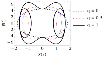
Figure 1: Phase diagram for a one-dimensional time-dependent harmonic oscillator, with $f_{0}=1$ and $g_{0}=0$. The $q=0$ case (dashed curve) represents the classical solution, while the solid curve shows the phase-space trajectory to $q=1$.

The representation of the corresponding phase-space to this solution can be view in Fig. 1. In this case, we can set the initial condition $x\left(0\right)=0$ and $p\left(0\right)=4.5,$ and the other parameters $\hbar=$ $m_{0}=\varepsilon_{0}=1$, $\omega_{0}=10$, $\eta_{0}=50$, $\varphi_{0}=-i$, $\nu=1/2$ are chosen as an example.

Note that, for $q>0$ found similar orbits in phase-space of those ion trajectories in Paul traps Trap . However, we want to stress that the limit case $q=0$ represented by the dashed curve, as shown in Fig. 1, reproduces the expected solution to simple harmonic motion.

Finally, we can now calculate the transition probability $P_{n}\left(\xi,\zeta\right)$ for the CSS by proceeding as discussed in previous sections. In Fig. 2, considering different values of $\tau$ can be viewed several transition probability from the Fock-states for the CSS, i.e., the probability to have $n$ number of excitations in the CSS.

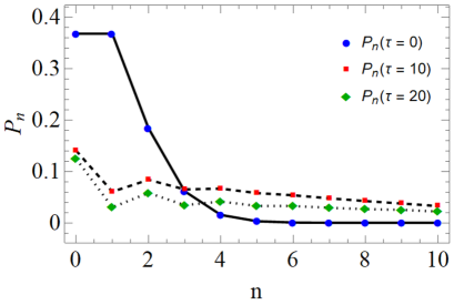
Figure 2: Transition probability distributions for the coherent squeezed states of the time-dependent harmonic oscillator for $\tau=0$, $10$, and $20$.

In this case, one can see that the distribution reached a maximum around the value $n=0$, for all $\tau$, and the transition probability does not keep its profile shape through time evolution.

VI Final Remarks

Given the recent interest the time-dependent systems in modern quantum mechanics and their potential applications in many fields, we have investigated the time-dependent displacement and squeezed parameters of the CSS. Following the integral of motion method, we have constructed integrals of motion for one-dimensional systems with general time-dependent quadratic Hamiltonian. By applying a nonunitary transformation, we find a direct relation between these integrals of motion $\hat{A}\left(t\right)$ and the canonical annihilation operator $\hat{a}$. In this context, one has calculated the corresponding CSS. As a consequence, we obtain the displacement $\xi\left(t\right)$ and squeezed parameters $\zeta\left(t\right)$ in terms of the functions $f\left(t\right)$, $g\left(t\right)$, and $\phi\left(t\right)$. We have related these parameters with those physical parameters present in the general quadratic Hamiltonian.

Moreover, by applying the nonunitary approach, one shown that CSS is annihilated by the integral of motion. Additionally, the Schrödinger equation of the system to the case under consideration is satisfied. We have also shown that the mean values of the phase-space variables, evaluate with respect to time-dependent CSS, satisfy Hamilton’s equations, and discussed conditions under which the uncertainty relation is minimized.

We show that, considering the integrals of motion method in the nonunitary approach, one can expand the time-dependent CSS on a time-independent Fock basis. Thus, we can analyze systems with finite-levels, and, therefore, there is potential for application in many fields of physics. This procedure ensures the possibility of generations of these states even for physical systems described by complex Hamiltonians.

Lastly, as an example, we described the solution to the general time-dependent harmonic oscillator driven by a time-dependent driving force. In this case, the phase diagram is presented and shown that, in limit case $q=0$, the simple harmonic motion solution is recovered. Finally, one has obtained the transition probability distributions that, as we showed, have not kept their profile shape through time evolution.

VII Acknowledgment

ASP thanks the support of the Instituto Federal do Pará. The authors would like to thank the referees for their valuable comments.

References

• (1) Klauder J R and Sudarshan E C 1968 Fundamentals of Quantum Optics (New York: Benjamin).
• (2) Scully M O and Zubairy M S 1997 Quantum Optics (Cambridge: Cambridge University Press).
• (3) Klauder J R and Skagerstam B S 1985 Coherent States, Applications in Physics and Mathematical Physics (Singapore: World Scientific).
• (4) Nielsen M and Chuang I 2000 Quantum Computation and Quantum Information (Cambridge: Cambridge University Press).
• (5) Glauber R J 1963 Coherent and incoherent states of the radiation field Phys. Rev. Lett. 10, 84.
• (6) Perelomov A 1986 Generalized Coherent States and Their Applications (Berlin: Springer).
• (7) Yuen H P 1976 Two-photon coherent states of the radiation field Phys. Rev. A 13, 2226.
• (8) Slusher R E and Yurke B 1990 Squeezed light for coherent communications J. Light. Tech. 8, 466.
• (9) Caves C M 1981 Quantum-mechanical noise in an interferometer Phys. Rev. D 23, 1693.
• (10) Ni W-T 1987 Quantum-mechanical noise in an interferometer: Intrinsic uncertainty versus measurement uncertainty Phys. Rev. D 35, 3002.
• (11) Chua S S Y, Slagmolen B J J, Shaddock D A and McClelland D E 2014 Quantum squeezed light in gravitational-wave detectors Class. Quant. Grav. 31, 183001.
• (12) Walls D F 1983 Squeezed states of light Nature 306, 141.
• (13) Fisher R A, Nieto M M and Sandberg V D 1984 Impossibility of naively generalizing squeezed coherent states Phys. Rev. D 29, 1107.
• (14) Satyanarayana M V 1985 Generalized coherent states and generalized squeezed coherent states Phys. Rev. D 32, 400.
• (15) Jannussis A and Bartzis V 1988 Coherent and squeezed states in quantum optics Nuo. Cim. B, 102, 33.
• (16) Nieto M M and Truax D R 2000 Higher-power coherent and squeezed states Opt. Commu. 179, 97.
• (17) Dodonov V V 2002 ‘Nonclassical’ states in quantum optics: a ‘squeezed’ review of the first 75 years J. Opt. B: Quantum Semiclass. Opt. 4, R1.
• (18) Dodonov V V and Man’ko V I 2003 Theory of Nonclassical States of Light (London: Taylor & Francis Group).
• (19) Pereira A S 2018 Coherent and semiclassical states of a charged particle in electromagnetic fields Braz. J. Phys. 48, 286.
• (20) Berry M V 1983 Quantal phase factors accompanying adiabatic changes Proc. R. Soc. Lond. A 392, 45.
• (21) Mizrahi S S 1989 The geometrical phase:An approach through the use of invariants physics Phys. Lett. A 138, 465.
• (22) Dodonov V V, Man’ko V I and Man’ko O V 1989 Correlated states in quantum electronics (resonant circuit) J. Sov. Laser Res. 10, 413.
• (23) Paul W 1990 Electromagnetic traps for charged and neutral particles Rev. Mod. Phys. 62, 531.
• (24) Agarwal G S and Kumar S A 1991 Exact quantum-statistical dynamics of an oscillator with time-dependent frequency and generation of nonclassical states Phys. Rev. Lett. 67, 3665.
• (25) Yeon K H, Um C I and George T F 2003 Time-dependent general quantum quadratic Hamiltonian system Phys. Rev. A, 68, 052108.
• (26) V G Bagrov, D M Gitman and A S Pereira 2015 Coherent states of systems with quadratic hamiltonians Braz. J. Phys. 45, 369.
• (27) Dodonov V V, Malkin I A and Man’ko V I 1972 Coherent states of a charged particle in a time-dependent uniform electromagnetic field of a plane current Physica 59, 241.
• (28) Dodonov V V, Malkin I A and Man’ko V I 1975 Integrals of the motion, green functions, and coherent states of dynamical systems Int. J. Theor. Phys. 14, 37.
• (29) Malkin I A and Man’ko V I 1979 Dynamical Symmetries and Coherent States of Quantum Systems (Moscow: Nauka).
• (30) Wünsche A 1992 Eigenvalue problem for arbitrary linear combinations of a boson annihilation and creation operator Ann. Physik 1, 181.
• (31) Roy A K and Mehta C L 1992 Squeezed states generated by boson creation operator J. Mod. Opt. 39, 1619.
• (32) Bremner M J, Dawson C M, Dodd J L, Gilchrist A, Harrow A W, Mortimer D, Nielsen M A and Osborne T J 2002 Practical Scheme for Quantum Computation with Any Two-Qubit Entangling Gate Phys. Rev. Lett. 89, 247902.
• (33) Nussenzveig H M 1973 Introduction to Quantum Optics (New York: Gordon and Breach).
• (34) Allen L and Eberly J H 1975 Optical Resonance and Two-Level Atoms (New York: Wiley).
• (35) Bagrov V G, Baldiotti M C, Gitman D M and Levin A D 2005 Spin equation and its solutions Ann. der Phy. 14, 764.
• (36) Erdélyi A 1953 Bateman Manuscript Project, Higher Transcendental Functions vol. 2 (New York: McGraw-Hill).
• (37) Pedrosa I A 1987 Comment on ”Coherent states for the time-dependent harmonic oscillator” Phys. Rev. D 36, 1279.
• (38) Robertson H P 1930 A general formulation of the uncertainty principle and its classical interpretation Phys. Rev. 35, 667.
• (39) Mclachlan N W 1947 Theory and application Mathieu functions (Oxford: Claredon Press).
• (40) Richards J A 1983 Analysis of periodically time-varying systems (Berlin: Springer-Verlag).
• (41) Major F G, Gheorghe V N and Werth G 2005 Charged particle traps: physics and techniques of charged particle field confinement (Berlin: Springer).