Consistency of invariance-based randomization tests

Abstract

Invariance-based randomization tests—such as permutation tests, rotation tests, or sign changes—are an important and widely used class of statistical methods. They allow drawing inferences under weak assumptions on the data distribution. Most work focuses on their type I error control properties, while their consistency properties are much less understood.

We develop a general framework and a set of results on the consistency of invariance-based randomization tests in signal-plus-noise models. Our framework is grounded in the deep mathematical area of representation theory. We allow the transforms to be general compact topological groups, such as rotation groups, acting by general linear group representations. We study test statistics with a generalized sub-additivity property. We apply our framework to a number of fundamental and highly important problems in statistics, including sparse vector detection, testing for low-rank matrices in noise, sparse detection in linear regression, and two-sample testing. Comparing with minimax lower bounds, we find perhaps surprisingly that in some cases, randomization tests detect signals at the minimax optimal rate.

1 Introduction

Invariance-based randomization tests—such as permutation tests—are an important, fundamental, and widely used class of statistical methods. They allow making inferences in general settings, with few assumptions on the data distribution. Most methodological and theoretical work focuses on their validity, studying their type I error (false positive rate) control. There is also work on their robustness properties, but less is known about their power and consistency properties.

Our work develops a general theoretical framework to understand the consistency properties of invariance-based randomization tests in signal-plus-noise models. In particular, we allow the randomization distributions to be Haar measures over general compact topological groups, such as rotation groups. We go beyond most prior work, which focuses on discrete groups (mainly permutation groups), and does not fully develop the technically challenging case of compact groups. Moreover, we allow the action of these groups on the data to be via arbitrary compact linear group representations.

We apply our theoretical framework to a number of fundamental and highly important problems in statistics, including sparse vector detection, low-rank matrix detection, sparse detection in linear regression, and two-sample testing. Perhaps surprisingly, we find that invariance-based randomization tests are minimax rate optimal in a number of cases. The reason why we consider this to be surprising is that the randomization tests are constructed using the same universal principle. They have only minimal information about the problem, namely a set of symmetries of the noise, and a test statistic that is expected to be “large” under the alternative.

In more detail, our contributions are as follows:

1. Representation-theoretic framework. We develop a framework for consistency of invariance-based randomization tests based on group representation theory. In our framework, we have a compact topological group that acts linearly on the data space. We assume that under the null hypothesis, distribution of the data is invariant under the action of the group. We sample several group elements chosen at random from the Haar measure on the group, and apply them to the data. We consider the standard invariance-based randomization test which rejects the null hypothesis when a chosen test statistic is larger than an appropriate quantile of the values of the test statistic applied to the randomly transformed data.

2. Consistency results. We develop consistency results for the invariance-based randomization test in signal-plus-noise models. We consider sequences of signal-plus-noise models where the signal equals zero under the null hypothesis. We study broad classes of test statistics satisfying the weak requirement of so-called $\psi$-subadditivity. This includes, for instance, suprema of linear functionals of the data, norms and semi-norms, concave non-decreasing functions in one dimension, convex functions of bounded growth. Further, this class is closed under conic combinations, taking maxima, and compositions with one-dimensional nondecreasing sub-additive functions.

   We develop a general consistency result, showing that if the sequence of alternatives is such that the value of the test statistic is large enough, then the test rejects with probability tending to unity. We compare this to the corresponding result for the deterministic test based on the same the statistic. The consistency threshold is inflated slighly by a signal-noise interference effect. By randomly transforming the signal, we create additional noise, inflating the effective noise level in the randomized statistic compared to its distribution under the null. However, we later show that in many examples this inflated noise level can be controlled. As part of our consistency theory, we extend to the setting with nuisance parameters, which allows us to handle problems such as two-sample testing.

3. New proof techniques. Our proofs are based on novel approaches. For the proofs of the general consistency result, we proceed by a series of reductions, first reducing from the quantile of the randomization distribution to its maximum, then from considering several random transformations to only one transform, and then reducing from a dependent transformed signal and noise to independent ones.

4. Examples. We illustrate our results in several important examples. We show that our results provide consistency conditions for invariance-based randomization tests in a number of problems, including sparse vector detection, low-rank matrix detection, sparse detection in linear regression, and two-sample testing.

   For sparse vector detection we consider two settings: where the noise vectors for the different observations are independent and sign symmetric (but not necessarily identically distributed), and where they are independent and rotationally symmetric (spherical). For both cases we obtain general consistency results, and some matching lower bounds. Specifically for the sign symmetric case where the entries of the noise are independent and identically distributed according to a sub-exponential distribution, our upper bound for the signflip randomization test matches a lower bound that we obtain. For spherical noise we obtain general upper bounds as well as specific examples for multivariate $t$ distributions. We also provide similar results for two sample testing.

   For low rank matrix detection, we consider the case where each of the columns of the noise matrix as an independent spherical distribution. We obtain a general upper bound for the operator norm test statistic, using the associated rotation test. We show that this result is rate optimal for the special case of normal noise.

   For sparse vector detection in linear regression, we study detection based on the $\ell_{\infty}$ norm of the least-squares estimator. We assume that the noise entries of each observation are independent and sign-symmetric. We provide a consistency result for the associated signflip based randomization test, in terms of geometric quantities determined by the feature matrix; namely the suprema of two associated Bernoulli processes.

As a general conclusion, we think it is perhaps surprising that invariance-based randomization tests can sometimes adaptively detect signals at the same rate as the optimal tests that assume knowledge about the exact noise distribution. We support our claims with numerical experiments.

Note on terminology. We follow the terminology of “randomization tests” from Ch. 15.2 of the standard textbook by Lehmann and Romano (2005): “the term randomization test will refer to tests obtained by recomputing a test statistic over transformations (not necessarily permutations) of the data.” This does not consider tests based on randomization of treatments; see e.g., Onghena (2018); Hemerik and Goeman (2020) for discussion. In particular, Hemerik and Goeman (2020) suggest using “randomization tests” only when the treatments are randomized, and suggest using “group invariance tests” for the type of tests we consider. For consistency with the standard textbook by Lehmann and Romano (2005), we will simply use the terminology “invariance-based randomization tests” or “randomization tests”. Another well-known example of randomization occurs with discretely distributed tests, to ensure exact type I error control; our work is unrelated to this issue.

Some notations. For a positive integer $m\geqslant 1$, the $m$-dimensional all-ones vector is denoted as $1_{m}=(1,1,\ldots,1)^{\top}$. We denote $[m]:=\{1,2,\ldots,m\}$, and for $j\in[m]$, the $j$-th standard basis vector by $e_{j}=(0,\ldots,1,\ldots,0)$, where only the $j$-th entry equals unity, and all other entries equal zero. The variance of a random variable $X$ is denoted as $\textnormal{Var}{X}$ or $\operatorname{Var}\left[X\right]$. For two random vectors $X,Y$, we denote by $X=_{d}Y$ that they have the same distribution. For an index $m=1,2,\ldots$, and two sequences $(a_{m})_{m\geqslant 1},(b_{m})_{m\geqslant 1}$, $a_{m}\lesssim b_{m}$ (and $a_{m}=O(b_{m})$) means that $a_{m}\leqslant Cb_{m}$ for some $C\geqslant 1$ independent of $m$, but possibly dependent on other problem parameters as specified case by case. We write $a_{m}\gtrsim b_{m}$ (or $a_{m}=\Omega(b_{m})$) when $b_{m}\lesssim a_{m}$, and $a_{m}\sim b_{m}$ (or $a_{m}=\Theta(b_{m})$) when $a_{m}\lesssim b_{m}\lesssim a_{m}$. For a vector $v\in\mathbb{R}^{m}$, and $p\in(0,\infty)$, $\|v\|_{p}$ denotes the $\ell_{p}$ norm. Unless otherwise specified, $\|v\|$ denotes the Euclidean or $\ell_{2}$ norm, $\|v\|=\|v\|_{2}$. For a matrix $s$, the norm $\|s\|_{2,\infty}$ is the maximum of the column $\ell_{2}$ norms of $s$. For two subsets $A,B$ of a vector space, $A+B=\{a+b:a\in A,b\in B\}$ denotes the Minkowski sum. For a $p\times 1$ vector $v$, let $M=\operatorname{diag}(v)$ be the $p\times p$ diagonal matrix with the entries $M_{ii}=v_{i}$. A function $f:V\mapsto V^{\prime}$, where $V,V^{\prime}$ are two vector spaces, is an odd function if $f(-v)=-f(v)$ for all $v\in V$. A Rademacher random variable is uniform over the set $\{\pm 1\}$. For a probability distribution $Q$ and a random variable $X\sim Q$, we may write probability statements involving $X$ in several equivalent ways, for instance for the probability that $X$ belongs to a measurable set $A$, we may write: $P(X\in A)$, $P_{X}(A)$, $P_{Q}(X\in A)$, $P_{X\sim Q}(X\in A)$, $Q(X\in A)$, or $Q(A)$. Further, if $Q$ belongs to a collection of probability measures $H$ (e.g., a null or an alternative hypothesis), then we may also write $P_{H}(A)$ to denote $Q(A)$ for an arbitrary $Q\in H$.

1.1 Related works

There is a large body of important related work. Here we can only review the most closely related ones due to space limitations. The idea of constructing a statistical test based on randomly chosen permutations of iid samples in a dataset dates back at least to Eden and Yates (1933); Fisher (1935), see David (2008); Berry et al. (2014) for historical details. General references on permutation tests include Pesarin (2001); Ernst (2004); Pesarin and Salmaso (2010b, 2012); Good (2006); Anderson and Robinson (2001); Kennedy (1995); Hemerik and Goeman (2018a). These tests have many applications, for instance in genomics (Tusher et al., 2001) and neuroscience (Winkler et al., 2014). For more general discussions of invariance in statistics see Eaton (1989); Wijsman (1990); Giri (1996); for a general probabilistic reference see also Kallenberg (2006).

Two-sample permutation tests date back at least to Pitman (1937b), and have recently been studied in more general multivariate contexts (Kim et al., 2020b). This problem brings special considerations such as issues with using balanced permutations (Southworth et al., 2009).

A number of invariance-based randomization based tests have been developed for linear and generalized linear models (Freedman and Lane, 1983; Perry and Owen, 2010; Winkler et al., 2014; Hemerik et al., 2020a). The works by Anderson and Legendre (1999); Winkler et al. (2014) review and compare a number of previously proposed permutation methods for inference in linear models with nuisance parameters. Hemerik et al. (2020b) show empirically that permutation tests can control type I error even in certain high dimensional linear models. Hemerik et al. (2020a) develop tests for potentially mis-specified generalized linear models by randomly flipping signs of score contributions.

Other specific problems where invariance-based randomization tests have been developed include independence tests (Pitman, 1937a), location and scale problems (Pitman, 1939), parallel analysis type methods for PCA and factor analysis (Horn, 1965; Buja and Eyuboglu, 1992; Dobriban, 2020; Dobriban and Owen, 2019), and time series data, where Jentsch and Pauly (2015) randomly permute entries between periodograms to test for equality of spectral densities. In addition, randomization based inference has been useful to study factorial designs (Pauly et al., 2015), regression kink designs (Ganong and Jäger, 2018), and linear mixed-effects models (Rao et al., 2019).

For the theoretical aspects of invariance-based randomization tests, Lehmann and Stein (1949) develop results for testing a null of equality in distribution $H_{m0}:X_{m}=_{d}g_{m}X_{m}$ where a transform $g_{m}\in\mathcal{G}_{m}$ is chosen from a group $\mathcal{G}_{m}$ acting on the data. They show that all admissible tests have constant rejection probability equal to the level over each orbit, i.e., are similar tests. They use this to show that the most powerful tests against simple alternatives with density $f_{m}$ reject when $f_{m}(X_{m})$ is greater than the appropriate quantile of $\{f_{m}(g_{m}X_{m}),g_{m}\in\mathcal{G}_{m}\}$. They use the Hunt-Stein theorem to derive uniformly most powerful (or most stringent) invariant tests from maximin tests for testing against certain composite alternatives. These are related to our results, but we focus on consistency against special structured signal-plus-noise alternatives instead of maximizing power in finite samples.

The seminal work by Hoeffding (1952) considers general group transforms, including signflips, for testing symmetry of distributions, but focuses on permutation groups for most part. The main results center on power and consistency of tests. For consistency, the main result (Theorem 2.1 in Hoeffding (1952)) states that for a test statistic $f_{m}$ such that $f_{m}(x)\geqslant 0$ and $\mathbb{E}_{G_{m}\sim Q_{m}}f_{m}(G_{m}x)\leqslant c$ where $G_{m}\sim Q_{m}$ denotes that the group element is distributed according to the probability measure $Q_{m}$ on $\mathcal{G}_{m}$, we have $q_{1-\alpha,m}(x)\leqslant c/\alpha$, $\alpha\in(0,1)$, where $q_{1-\alpha,m}$ is the $1-\alpha$-th quantile of the distribution of $f_{m}(G_{m}x)$ when $G_{m}\sim Q_{m}$. Then, if $f_{m}\to\infty$ under a sequence of alternatives, the test that rejects when $f_{m}>q_{1-\alpha,m}(x)$ is consistent, i.e. has power tending to unity. These conditions are distinct from ours. Specifically, his conditions require the test statistic to be pointwise bounded (for each datapoint $x$, they require that $\mathbb{E}_{G_{m}\sim Q_{m}}f_{m}(G_{m}x)\leqslant c$), whereas our conditions are high probability bounds in terms of the randomness over both the data and the random transform. Thus, the two types of conditions are different. Our condition does not even require that the expectation $\mathbb{E}_{G_{m}\sim Q_{m}}f_{m}(G_{m}x)$ is finite, and thus are applicable to heavy-tailed distributions.

For asymptotic power of certain special invariance-based randomization tests, one can obtain results based on contiguity, see e.g., Example 15.2.4 in Lehmann and Romano (2005). However, we are interested in problems where the contiguity of the alternatives may be unknown, or hard to establish.

For permutation tests, Dwass (1957) shows that it is valid to randomly sample permutations—as opposed to using all permutations—to construct the randomization test. Hemerik and Goeman (2018b) provide a general type I error control result for random group transformations under exact invariance, and apply it to false discovery proportion control. See also Hemerik et al. (2019). Hemerik and Goeman (2018a) extend this in various forms, including to sampling transforms without replacement, and giving rigorously justified formulas for $p$-values.

Most works assume exact invariance of the distribution. Romano (1990) studies the behavior of invariance-based randomization tests beyond the exact group invariance framework. This work shows that asymptotic validity holds in certain cases, and fails in others. Canay et al. (2017) relax assumptions to only require invariance in distribution of the limiting distribution of the test statistic. They show that the group randomization test has an asymptotically correct level.

Chung and Romano (2013) develop general permutation tests with finite-sample error control based on studentization. Further studies include discussions of conditioning on sufficient statistics (Welch, 1990), combination methods (Pesarin, 1990), and others (Janssen and Pauls, 2003; Kim et al., 2020a).

Beyond permutation tests, flipping signs is considered in many works, see e.g., Pesarin and Salmaso (2010b). Following Wedderburn (1975), Langsrud (2005) discusses rotation tests in Gaussian linear regression. This approach assumes data $X_{m}\sim\mathcal{N}(0,I_{p_{m}}\otimes\Sigma_{m})$, and computes the values of test statistics on $X_{R}=R_{m}X_{m}$, where $R_{m}$ are uniformly distributed orthogonal matrices over the symmetric group $O(p_{m})$. This is applied to testing independence of two random vectors, as well as to more general tests in multivariate linear regression. Perry and Owen (2010) extends the method to verify latent structure. Solari et al. (2014) argues for the importance of this method in multiple testing adjusting for confounding. The theoretical aspects of rotation tests for sphericity testing of densities are discussed briefly by Romano (1989), Proposition 3.2.

Toulis (2019) develops residual invariance-based randomization methods for inference in regression. This work considers a general invariance assumption $\varepsilon_{m}=_{d}g_{m}\varepsilon_{m}$ for the noise $\varepsilon_{m}$, for all group elements $g_{m}\in\mathcal{G}_{m}$. For ordinary least squares (OLS), it considers the test statistic $t(\hat{\varepsilon}_{m})=a^{\top}(X_{m}^{\top}X_{m})^{-1}X_{m}^{\top}g_{m}\hat{\varepsilon}_{m}$, where $\hat{\varepsilon}_{m}$ are the OLS residuals, and $a$ is a vector. This work discusses many examples, including clustered observations such that the noise is correlated within clusters, proposing to flip the signs of the cluster residuals.

There are a number of works studying the power properties of invariance-based randomization tests. We have already discussed the fundamental work by Hoeffding (1952). Pesarin and Salmaso (2010a) develop finite-sample consistency results for certain combination-based permutation tests for multivariate data, when the sample size is fixed and the dimension tends to infinity. They focus on one-sided two-sample tests, and discuss Hotelling’s $T$-test as an example. Pesarin and Salmaso (2013) characterize weak consistency of permutation tests for one-dimensional two-sample problems. They study stochastic dominance alternatives assuming the population mean is finite and without assuming existence of population variance.

Pesarin (2015) develops some further theoretical aspects of permutation tests. This includes consistency properties (Property 9), for two-sample tests under some non-parametric assumptions, and alternatives specified by an increased mean of the test statistic. These have different assumptions than the results in our paper, focusing on two-sample problems (while we have general invariance), and non-parametric models (while we focus on parametric ones).

One one of the most closely related papers is that of Kim et al. (2020a). We discuss the similarities and differences. The methodology of permutation tests is a special case of general group invariance tests; however the examples in our work mostly concern sighflip-based and rotation tests. The only overlap in the specific problems studied is for two-sample testing, but under different assumptions (we study testing the equality of means in a location model, whereas they study testing the equality of two distributions such as multinomials and distributions with Holder densities). Thus our results are not directly comparable. For instance our minimax optimality for two-sample testing involves location families with IID sub-exponential noise, whereas their examples are multinomial distributions and Holder densities.

In context. To put our work in context, we can make the following comparisons:

• The vast majority of works only provide theoretical results for the behavior of randomization tests under the null hypothesis (Eden and Yates, 1933; Fisher, 1935; Pitman, 1939; Hemerik and Goeman, 2018a).

• The seminal work of Hoeffding (1952), already discussed above, provides consistency conditions that are distinct from ours; and does not discuss any of the specific problems that we study. The power analysis based on contiguity (Lehmann and Romano, 2005) does not apply to many of the problems we study. As detailed above, the consistency and minimax optimality analyses from Pesarin and Salmaso (2010a, 2013); Pesarin (2015); Kim et al. (2020a) all concern different setups from and/or special cases of our results.

Scientific context. For an even broader scientific context, we emphasize that randomization tests are ubiquitous in modern science. Their proper use is crucial for reproducible results; and failure to use them correctly can result in irreproducible results, false scientific discoveries, and ultimately a waste of resources. Here are some examples:

• In neuroscience, the analysis of fMRI data requires testing hypotheses about the activation of regions in the brain. It has been observed that inferences based on models such as Gaussian fields with parametric covariance functions can have massively inflated false-positive rates (Eklund et al., 2016). To mitigate this problem, it has been proposed to use randomization methods such as permutation methods (for two-sample problems) or random sign flips (for one sample problems) to set critical values. Further randomization methods have been proposed for other problems such as general linear models (Winkler et al., 2014), or brain network comparison (Simpson et al., 2013).
  The ultimate goal is to report reliable discoveries, which involves analyzing data not from the null distribution, but rather from an alternative distribution that contains signals. Our work can shed light on when using randomization tests in such an analysis from data containing signals can succeed.

• In genetics and genomics, hypothesis testing is routinely performed to identify associations between observed phenotypes and genotypes, or between genotypes, etc. Randomization tests, and in particular permutation tests, are widely used to set critical values, in methods such as transmission disequilibrium tests, etc, and are broadly available in popular software such as PLINK, see for instance Churchill and Doerge (1994); Purcell et al. (2007); Epstein et al. (2012). Randomization tests are also used for more sophisticated tasks such as gene set enrichment analysis (Subramanian et al., 2005; Barry et al., 2005; Efron and Tibshirani, 2007).

2 General framework

2.1 Setup

We consider a sequence of statistical models, indexed by an index parameter $m\to\infty$. We observe data $X_{m}$ from a real vector space $V_{m}$, for instance a vector or a matrix belonging to Euclidean space $\mathbb{R}^{p_{m}}$. We assume that we know a group $\mathcal{G}_{m}$ of the symmetries of the distribution of the data. See Section 5.1 for a discussion of how is can arise in practice. A group $\mathcal{G}_{m}$ has a multiplication operation $"\cdot"$ that satisfies the axioms of associativity, identity, and invertibility. For instance, we could have that the entries of $X_{m}$ are exchangeable (corresponding to the permutation group), symmetric about zero (corresponding to the group of addition modulo two) or that the density of $X_{m}$ is spherical (corresponding to the rotation group).

In addition, to transform the data, we have a group representation $\rho_{m}:\mathcal{G}_{m}\to GL_{m}(V_{m})$, acting linearly on $X_{m}\in V_{m}$ via $g_{m}X_{m}:=\rho_{m}(g_{m})\cdot X_{m}$. The group representation “represents” the elements of the group $\mathcal{G}_{m}$ as invertible linear operators $V_{m}\mapsto V_{m}$ belonging to the general linear group $GL_{m}(V_{m})$ of such operators. The group representation $\rho_{m}$ preserves the group multiplication operation, i.e., $\rho_{m}(g_{m}g_{m}^{\prime})=\rho_{m}(g_{m})\rho_{m}(g_{m}^{\prime})$ for all $g_{m},g_{m}^{\prime}\in\mathcal{G}_{m}$, and $\rho_{m}(e_{\mathcal{G}_{m}})=I_{V_{m}}$, where $e_{\mathcal{G}_{m}}$ is the identity element of the group, and $I_{V_{m}}$ is the identity operator on $V_{m}$. For general references on representation theory, see Serre (1977); James and Liebeck (2001); Fulton and Harris (2013); Hall (2015); Knapp (2013); Eaton (1989), etc. For group representations in statistics, see Diaconis (1988). We will use basic concepts from this area throughout the paper.

Null hypothesis of invariance, and randomization test. We want to use the symmetries of the noise distribution to detect the presence of non-symmetric signals. Under the null hypothesis, we assume that the distribution of the data is invariant under the action of each group element $g_{m}\in\mathcal{G}_{m}$: $X_{m}=_{d}g_{m}X_{m}$. We study the following invariance-based randomization test (sometimes also called a group invariance test), which at various levels of generality has been considered dating back to Eden and Yates (1933); Fisher (1935); Pitman (1937b); Lehmann and Stein (1949); Hoeffding (1952). We sample $G_{m1},\ldots,G_{mK}$ iid from $\mathcal{G}_{m}$ (in a way specified below), and reject the null if for a fixed test statistic $f_{m}:V_{m}\mapsto\mathbb{R}_{m}$, the following event holds

$$\mathcal{E}_{m}=\{f_{m}(X_{m})>q_{1-\alpha}\left(f_{m}(X_{m}),f_{m}(G_{m1}X_{m}),\ldots,f_{m}(G_{mK}X_{m})\right)\},$$ (1)

for the $1-\alpha$-th quantile $q_{1-\alpha}$ of the numbers $\{f_{m}(X_{m}),f_{m}(G_{m1}X_{m}),\ldots,f_{m}(G_{mK}X_{m})\}$ and some $\alpha\in(0,1]$. Specifically, let $G_{m0}=I_{V_{m}}$ be the identity operator on $V_{m}$, and $f_{(1)}\leqslant f_{(2)}\leqslant\ldots\leqslant f_{(K+1)}$ be the ordered test statistics of the set $\{f_{m}(G_{mi}X_{m}),i\in\{0,1,\ldots,K\}\}$. Let $k=\lceil(1-\alpha)(K+1)\rceil$. Rejecting the null if $f_{m}(X_{m})>f_{(k)}$ is guaranteed to have level at most $\alpha$, see e.g., theorem 2 in Hemerik and Goeman (2018a) for an especially clear and rigorous statement. In some cases, one can relax this to assume only $f_{m}(X_{m})=_{d}f_{m}(g_{m}X_{m})$ under the null, see e.g., Canay et al. (2017); Hemerik and Goeman (2018a), but we will not pursue this.

Noise invariance and robustness. The advantage of randomization tests compared to a rejection region of the form $f_{m}(X_{m})>\tilde{c}_{m}$ for a fixed $\tilde{c}_{m}$ is that it does not require the manual specification of the critical value $\tilde{c}_{m}$. The critical value needs to account for the set of distributions included the null hypothesis, which may be a very large nonparametric family. In this case, it might be challenging to set the critical value to ensure type I error control. Randomization tests avoid this problem by relying on the symmetries of the noise distributions. To wit, randomization tests are valid under any null hypothesis for which the distribution of the noise is invariant under the group. This effectively amounts to that only depend on the collection of orbits, which form a maximal invariant of the group, see Sections 3 and 4 in Eaton (1989) for examples.

For instance, for the rotation group $O(p_{m})$, we get spherical distributions, which have a density $p_{m}(X_{m})=\pi_{m}(\|X_{m}\|_{2})$ with respect to a $\sigma$-finite dominating measure on $\mathbb{R}^{p_{m}}$ only depending on the Euclidean norm of the data $X_{m}$ (Kai-Tai and Yao-Ting, 1990; Gupta and Varga, 2012; Fang et al., 2018). This is a non-parametric class that includes in particular distributions such as the multivariate $t$, multivariate Cauchy, scale mixtures of spherical normals etc. In particular, it includes heavy tailed distributions, for which tests based on the normal assumption can have inflated type I error. As another example, consider a stationary field $X_{m,J}=(X_{i})_{i\in J}$, for some index set $J$. Suppose $\mathcal{G}_{m}$ acts on $J$, and induces an action on $X_{m,J}$ via its regular representation, i.e., $(g_{m}X_{m,J})_{i}=X_{g_{m}^{-1}i}$. For instance, we can have a discrete-time stationary time series where $J=\mathbb{Z}$, and $\mathcal{G}_{m}=(\mathbb{Z},+)$. In this example, any translation of the time series keeps the distribution invariant; but this allows a wide range of noise distributions.

While sometimes it is possible to construct test statistics whose distribution does not depend on a broad set of null hypotheses (see e.g., Section 4.3 “Null robustness” in Eaton (1989)), this may not be possible when the null hypothesis has a great number of nuisance parameters. For example, this holds for null hypotheses where each noise entry is independent with a probability density only assumed to be symmetric around zero, in which case sign-flip based methods are applicable, see e.g., Example 15.2.1 of Lehmann and Romano (2005), and also Hemerik et al. (2020a); Hong et al. (2020).

Haar measure. In the definition of the randomization test, $G_{m1},\ldots,G_{mK}$ are chosen iid from the uniform (Haar) measure on $\mathcal{G}_{m}$, which is assumed to exist. We refer to Section 2 in Folland (2016) for details, see also Fulton and Harris (2013); Eaton (1989); Wijsman (1990). Thus, $\mathcal{G}_{m}$ is assumed to be a compact Hausdorff topological group with the Borel sigma-algebra generated by the open sets. For brevity, we will sometimes refer to such groups as compact groups. The Haar probability measure $Q_{m}$ on $\mathcal{G}_{m}$ is the unique probability measure such that $Q_{m}(G_{m}\in A)=Q_{m}(G_{m}\in g_{m}^{\prime}A)$ for all $g_{m}^{\prime}\in\mathcal{G}_{m}$ and for all Borel sets $A_{m}$. See e.g., Theorems 2.10 & 2.20 in Folland (2016). Thus, in particular, we have the equality in distribution $G_{m}=_{d}G_{m}g_{m}^{\prime}$ for $G_{m}\sim Q_{m}$, and any fixed $g_{m}^{\prime}\in\mathcal{G}_{m}$.

Choice of $K$. We remark that, as is well known, choosing $K$ larger, and $k$ as above, can generally lead to a more precise control of the type I error. Indeed, for a given $K$, the smallest type I error control guaranteed by the randomization test is $1/(K+1)$, and there are only $K$ possible values of $k\in[K]$ to control the type I error more generally. Thus, for a larger $K$, we expect that we can control the type I error more accurately. Indeed, we observe this in our experiments.

Alternative hypothesis: signal-plus-noise model. To study the consistency of the test, we will consider a sequence of alternative hypotheses in the signal-plus-noise model with a deterministic signal $s_{m}$ and a random noise $N_{m}$

$$X_{m}=s_{m}+N_{m}.$$

The null hypothesis is specified by $H_{m0}:s_{m}=0_{p_{m}}$, in which case $X_{m}=N_{m}$. The alternative hypothesis $H_{m1}$ is specified by a set $\Theta_{m1}\subset V_{m}$ of signals $s_{m}\in\Theta_{m1}$. We call $\Theta_{m}=\{0\}\cup\Theta_{m1}$ the parameter space. The alternative hypothesis is decisively not invariant under $\mathcal{G}_{m}$. In fact, one can view the test statistic as detecting deviations from invariance.

We view the signal-plus-noise model as quite broad, and we will study a variety of examples as special cases. The breadth of the model arises from two aspects: First, one can choose the signal parameter space $\Theta_{m}$ to be quite general, for instance a linear subspace, a union of linear subspaces, a convex cone, etc. Second, one can model the family to which the distribution of the noise $N_{m}$ belongs; and our theory will rely on the symmetries of these distributions. Further, based on finite-dimensional asymptotic statistics, we know that asymptotically any sufficiently regular parametric model is well approximated by a normal observation model, which can be viewed as a signal-plus-noise model like ours if the noise distribution does not depend on the signal.

However, the scope of this model is limited in a few ways. It assumes a specific “structural model” for the data, and it is essentially a submodel of a multi-dimensional location family. For instance, it requires the distribution of the noise to be functionally independent on the unknown paramater $s_{m}$. In some cases, this may be approximately achieved via appropriate variance-stabilizing transforms. In our analysis, this is currently needed to be able to formulate consistency conditions based on only one global distribution of the noise. If the noise distribution can vary in parameter space, we expect that the behavior of randomization tests could be more complex. We discuss this and further limitations of our work in Section 4.

2.2 General consistency

Our basic idea to establish consistency of randomization tests is to find conditions under which the test statistic under the alternative is much larger than the randomized test statistic, i.e., (informally) $f_{m}(s_{m}+N_{m})\gg f_{m}(G_{m}[s_{m}+N_{m}])$. We wish to do this by introducing only broadly applicable assumptions. The first key step is to find a lower bound on $f_{m}(s_{m}+N_{m})$. To achieve this, we make assumptions of $f_{m}$.

For a given constant $\psi>0$, we consider $\psi$-subadditive test statistics, i.e., functions $f_{m}:V_{m}\mapsto\mathbb{R}$ such that for all $a,b\in V_{m}$,

$$\psi\cdot f(a+b)\leqslant f(a)+f(b).$$

Note that typically $\psi\leqslant 1$. In the current argument, we will use that $f_{m}(s_{m}+N_{m})\geqslant\psi f_{m}(s_{m})-f_{m}(-N_{m})$. This allows us to lower bound the value $f_{m}(s_{m}+N_{m})$ of the test statistic by a main term $\psi f_{m}(s_{m})$ depending only on the signal, and an error term $-f_{m}(-N_{m})$ depending only on the noise (which we will also control). We will use a similar argument to upper bound the randomized test statistic $f_{m}(G_{m}[s_{m}+N_{m}])$. These conditions are enough to guarantee the consistency of tests of the form $f_{m}(X_{m})>\tilde{c}_{m}$ for appropriately chosen “oracle” critical values $\tilde{c}_{m}$ (which are not practically implementable in general); and we will compare the resulting conditions later in this section.
Examples of subadditive functions include:

1. Given any set $W_{m}\subset V_{m}$, the suprema of linear functionals

   $$f_{m}(x)=\sup_{w_{m}\in W_{m}}w_{m}^{\top}x,$$

   assumed to be finite-valued functions, are $1$-subadditive. These are the sublinear functionals on $V_{m}$, see e.g., Sect 5.4, Ch 7, and specifically Exercise 7.103 in Narici and Beckenstein (2010). In particular, affine functions $f(x)=w^{\top}x+c$ are $1$-subadditive for any $w\in V_{m}$ and any $c\geqslant 0$.

2. For instance, for any norm $\|\cdot\|$ on $V_{m}$ (with the dependence on $m$ suppressed), we can take $f_{m}(x)=\|x\|$ by choosing $W_{m}=\{w_{m}:\|w_{m}\|_{*}\leqslant 1\}$, the unit ball in the dual norm $\|\cdot\|_{*}$ of $\|\cdot\|$.

3. When $V_{m}=\mathbb{R}$ is one-dimensional, for any concave non-decreasing function $c:[0,\infty)\to\mathbb{R}$ such that $c(0)\geqslant 0$, $f:\mathbb{R}\mapsto\mathbb{R}$ given by $f(x)=c(|x|)$ is $1$-subadditive. Examples include $f(x)=|x|^{q}$ for $q\in(0,1]$. See Section 5.2.1 for the argument.

4. Convex functions of bounded growth: If $f:\mathbb{R}^{p}\to\mathbb{R}$ is convex and satisfies $\psi f(2x)\leqslant 2f(x)$, then $f$ is $\psi$-subadditive. Indeed, $f(a)+f(b)\geqslant 2f([a+b]/2)\geqslant\psi f(a+b)$ by convexity and bounded growth. For instance, $f(x)=\|x\|_{q}^{q}$, for $q\geqslant 1$ satisfies $f(2x)=2^{q}f(x)$, thus it is $2^{1-q}$-subadditive.

Non-examples include functions of very fast growth, for instance $f:\mathbb{R}\mapsto\mathbb{R}$, $f(x)=\exp(x)$. However, for the purposes of hypothesis testing, only the acceptance and rejection regions are relevant; and thus even for test statistics that are not subadditive, one may—on a case-by-case basis—find sub-additive test statistics with the same acceptance and rejection regions; where our theory can be applied. For instance, instead of the exponential map above, one may consider the identity map.
Further, this class has a number of closure properties, being closed under:

1. Conic combinations: If $f_{j}:V_{j}\mapsto[0,\infty)$, $j\in[J]$ are $\psi_{j}$-subadditive, then for any $\tau_{j}\geqslant 0$, $j\in[J]$, $\sum_{j\in[J]}\tau_{j}f_{j}$ is $\min_{j\in[J]}\psi_{j}$-subadditive.

2. Maxima: If $f_{j}:V_{j}\mapsto[0,\infty)$, $j\in[J]$ are $\psi_{j}$-subadditive, then $\max_{j\in[J]}f_{j}$ is $J^{-1}\min_{j\in[J]}\psi_{j}$-subadditive.

3. Compositions with 1-D functions: if $f_{1}:[0,\infty)\mapsto\mathbb{R}$ is non-decreasing and $\psi_{1}$-subadditive; and $f_{2}:\mathbb{R}^{p}\mapsto[0,\infty)$ is $1$-subadditive, then $f_{1}\circ f_{2}:\mathbb{R}^{p}\mapsto\mathbb{R}$ is $\psi_{1}$-subadditive. Indeed,

   $$f_{1}\circ f_{2}(x+y)\leqslant f_{1}[f_{2}(x)+f_{2}(y)]\leqslant\psi_{1}^{-1}[f_{1}\circ f_{2}(x)+f_{1}\circ f_{2}(y)].$$

Our first theorem is a general consistency result for randomization tests with $\psi$-subadditive test statistics.

Theorem 2.1 (Consistency of randomization test).

Consider a sequence of models indexed by $m\geqslant 1$, $m\in\mathbb{N}$, such that the data $X_{m}\in V_{m}$ follow a $p_{m}$-dimensional signal-plus-noise model $X_{m}=s_{m}+N_{m}$, where $s_{m}\in\Theta_{m}$ is deterministic and $N_{m}$ is a random noise vector. Test the sequence of null hypotheses $H_{m0}:s_{m}=0$ against a sequence of alternative hypotheses $H_{m1}$ with signal vectors $s_{m}\in\Theta_{m1}$ for a fixed $\alpha\in(0,1]$. Reject the null hypothesis using the randomization test (1). Let $f_{m}$ be $\psi$-subadditive. Assume the following:

1. Noise invariance. The distribution of the noise is invariant under $\mathcal{G}_{m}$: $N_{m}=_{d}g_{m}N_{m}$ for all $g_{m}\in\mathcal{G}_{m}$.

2. Signal strength. There is a sequence $(t_{m})_{m\geqslant 1}$, and for any sequence $(s_{m})_{m\geqslant 1}$ such that for all $m\geqslant 1$, $s_{m}\in\Theta_{m1}$, there is another sequence $(\tilde{t}_{m})_{m\geqslant 1}$, $\tilde{t}_{m}=\tilde{t}_{m}(s_{m})$, such that for all large enough integers $m$,

   $${f_{m}(s_{m})>\psi^{-2}\tilde{t}_{m}(s_{m})+\psi^{-1}(\psi^{-1}+1)t_{m}}.$$ (2)

   Further, as $m\to\infty$,

   1. Noise level. $P(f_{m}(N_{m})\leqslant t_{m})\to 1$ and $P(f_{m}(-N_{m})\leqslant t_{m})\to 1$.

   2. Bound on randomized statistic. The test statistics evaluated on the randomized signal fall below $\tilde{t}_{m}(s_{m})$, i.e., for any sequence $(s_{m})_{m\geqslant 1}$ such that for all $m\geqslant 1$, $s_{m}\in\Theta_{m1}$,

      $${P_{G_{m}\sim Q_{m}}(f_{m}(G_{m}s_{m})\leqslant\tilde{t}_{m}(s_{m}))\to 1}.$$

Under condition 1, the randomization test has level at most $\alpha$. Under conditions 1& 2, the randomization test is consistent, i.e., for the event $\mathcal{E}_{m}$ from (1), for any sequence $(s_{m})_{m\geqslant 1}$ such that $s_{m}\in\Theta_{m1}$ for all $m\geqslant 1$, $\lim_{m\to\infty}P_{G_{m1},\ldots,G_{mK}\sim Q_{m},N_{m}}(\mathcal{E}_{m})=1$.

Some comments on the assumptions are in order:

1. The noise invariance condition is required to ensure the exact type I error control, as discussed above.

2. Our analysis relies on comparing the size of the test statistic on the data and the randomized data. The sub-additivity assumption allows us to reduce this to comparing the size of the test statistics on the signal, the noise, and the randomized signal. The remaining conditions are meant to capture high-probability deterministic bounds on the statistic over the randomness in the remaining stochastic quantities: the noise and random group elements.

3. The sequence $t_{m}$ controls the size of the statistic $f_{m}$ evaluated on the noise $N_{m}$. The sequence $\tilde{t}_{m}(s_{m})$ controls the size of the statistic evaluated on the randomized signal $G_{m}s_{m}$.

See Section 5.2.2 for the proof, which is novel. For the consistency result, we proceed by a series of reductions, first reducing from the quantile test to a max-based test, then from considering several random transformations to only one transform, and then reducing from a dependent transformed signal and noise to independent ones.

Conventions. To lighten notation, we will often omit the dependence of $\tilde{t}_{m}(s_{m})$ on $s_{m}$, writing simply $\tilde{t}_{m}$. Further, when it is clear from context what the sequence of tests is, we will simply say that the “test is consistent”, as opposed to saying that the “sequence of tests is consistent”.

Consistency of deterministic test. As mentioned, $\psi$-subadditivity is enough to guarantee the consistency of tests of the form $f_{m}(X_{m})>\tilde{c}_{m}$ for appropriately chosen critical values $\tilde{c}_{m}$. We state this result below and compare it as a “baseline” result with the conditions for the consistency of randomization tests.

Proposition 2.2 (Consistency of deterministic test).

In the setting of Theorem 2.1, suppose that condition 2(a) holds, along with the following condition:

1. Signal strength. There is a sequence $(t_{m})_{m\geqslant 1}$ such that for all large enough integers $m\geqslant 1$,

   $$f_{m}(s_{m})>2\psi^{-1}t_{m}.$$ (3)

Then, for any sequence $(\tilde{c}_{m})_{m\geqslant 1}$ such that $\tilde{c}_{m}\leqslant t_{m}$ for all $m\geqslant 1$, the sequence of deterministic tests that rejects when $f_{m}(X_{m})>\tilde{c}_{m}$ is consistent, i.e., $\lim_{m\to\infty}P_{H_{m1}}(f_{m}(X_{m})>\tilde{c}_{m})=1$.

See Section 5.2.3 for the proof. To ensure type I error control at level $\alpha$, the sequence $(\tilde{c}_{m})_{m\geqslant 1}$ needs to be chosen such that $\sup_{P\in H_{m0}}P(f_{m}(X_{m})>\tilde{c}_{m})\leqslant\alpha$. As we discussed, this can be difficult when the class of null hypotheses is large and has many nuisance parameters. Thus, the deterministic test may not be practically implementable. However we can still consider it as an idealized “baseline”, to understand the conditions on the signal strength that our approach provides to ensure consistency. Comparing the conditions for data signal strength, (2) and (3), and recalling that typically $\psi\leqslant 1$, we see that the requirement for the randomization test is stronger. The factor in front the noise level $t_{m}$ is larger, and in addition the randomization test also has the additional term $\psi^{-2}\tilde{t}_{m}$ controlling the size of the randomized signal.
Thus, our requirements for the randomization test are more stringent. However, as explained above, the randomization test requires a method to set the critical value, which may be very hard or impossible in practice in certain problems where the null hypothesis is very large.

Nuisance parameters. We next develop a generalization of our consistency results allowing nuisance parameters. This allows handling problems such as two-sample testing where the global mean is a nuisance. Let $X_{m}=\nu_{m}+s_{m}+N_{m}$, where $\nu_{m}$ is a nuisance parameter, $s_{m}\in\Theta_{m}$ is the signal. Suppose $\nu_{m}$ belongs to a known linear space $U_{m}$, $\nu_{m}\in U_{m}$. We can reduce this to the previous setting by projecting into the orthogonal complement of $U_{m}$. Let $P_{m}=P_{U_{m}^{\perp}}$ be the orthogonal projection operator into the orthogonal complement of $U_{m}$. Then $P_{m}\nu_{m}=0$, so by projecting with $P_{m}$, we have

$$P_{m}X_{m}=P_{m}s_{m}+P_{m}N_{m}.$$

Let $\tilde{X}_{m}=P_{m}X_{m}$ be the new observation, $\widetilde{S}_{m}=P_{m}s_{m}$ be the new signal, and $\widetilde{N}_{m}=P_{m}N_{m}$ be the new noise. Then, this reduces to the standard signal-parameter model, with the signal parameter space $\widetilde{\Theta}_{m}=P_{m}\Theta_{m}=\{P_{m}s_{m}:s_{m}\in\Theta_{m}\}$, and a new induced noise distribution.

2.3 Review of tools to obtain concrete results

To analyze concrete examples, we will rely on a few technical tools, reviewed in the following sections.

2.3.1 Rate optimality

In this section, we review some basic results on minimax rate optimality for hypothesis testing that we will use, focusing on Ingster’s (or the chi-squared) method (Ingster, 1987; Ingster and Suslina, 2012). This result allows randomized tests $\phi:V_{m}\mapsto[0,1]$, where $\phi(x)$ is the probability of rejecting the null for data $x$. Denote the set of all level $\alpha\in(0,1)$ tests by

$$\Phi_{m}(\alpha)=\left\{\phi:V_{m}\mapsto[0,1]:\sup_{P\in H_{m0}}\mathbb{E}_{P}[\phi]\leq\alpha\right\}.$$

Define the minimax type II error as

$$R_{m}=\inf_{\phi\in\Phi_{m}(\alpha)}\sup_{P\in H_{m1}}\mathbb{E}_{P}[1-\phi].$$

Suppose that $P_{m0}\in H_{m0}$ and $P_{m1}$, $\dots,P_{mM_{m}}\in H_{m1}$. Define the average likelihood ratio between $P_{m0}$ and $P_{m1}$, $\dots,P_{mM_{m}}$ as

$$L_{m}=\frac{1}{M_{m}}\sum_{i=1}^{M_{m}}\frac{p_{mi}(X_{m})}{p_{m0}(X_{m})},$$

where $p_{mi}$, $i\in[M_{m}]\cup\{0\}$ are, respectively, the densities of $P_{mi}$, $i\in[M_{m}]\cup\{0\}$ with respect to a common dominating sigma-finite measure on $V_{m}$. Then, it is well known (see e.g., Ingster and Suslina (2012), and Section III.B of Banks et al. (2018) for a very clear statement) that to achieve consistency, i.e., to have $R_{m}\to 0$, we must have $\lim_{m\to\infty}$ $\textnormal{Var}_{P_{m0}}[L_{m}]=\infty$.
A further key result holds when the null distribution $P_{m0}$ is $\mathcal{N}(0,I_{p_{m}})$ and the alternative $H_{m1}$ contains distributions of the form $\mathcal{N}(s_{m},I_{p_{m}})$, for $s_{m}\in\Theta_{m1}$. Consider a prior $\Pi_{m}$ on $\Theta_{m1}$. Then, we have, see e.g., Ingster and Suslina (2012) or Lemma 1 of Banks et al. (2018), for two independent copies $S,S^{\prime}\sim\Pi_{m}$,

$$\textnormal{Var}_{P_{m0}}[L_{m}]=\mathbb{E}_{S,S^{\prime}\sim\Pi_{m}}\exp(S^{\top}S^{\prime}).$$ (4)

2.3.2 Tail bounds of random variables

We recall some well known tail bounds for random variables. Suppose that for all $m\geqslant 1$ and $i\in[m]$, $Z_{i}$ are iid random variables with a probability distribution $\pi$. Let $F_{\pi}(t,n)=P(|n^{-1}\sum_{i=1}^{n}Z_{i}|>t)$, with $Z_{i}\sim\pi$ iid for all $i\in[n]$.
There is a vast number of well-known results on tail bounds of sums of iid random variables under a variety of conditions, see e.g., Petrov (2012); Boucheron et al. (2013); Vershynin (2018), etc. Each of these can be used together with our framework to obtain consistency results. In a very rough order of increasing generality:

1. The tail of sums of sub-exponential random variables (including sub-gaussian and bounded variables) can be controlled via Bernstein-type inequalities, which lead to $F_{\pi}(t,n)\leqslant$ $C\exp(-cn\min\{t,t^{2}\})$ for some $C,c$ depending only on $\pi$ (Vershynin, 2018). Bernstein-Orlicz random variables interpolate between sub-Gaussian and sub-exponential random variables (van de Geer and Lederer, 2013).

2. There are various Orlicz norms for random variables, and corresponding tail bounds, for instance for random variables with tail decay of order roughly $\exp(-x^{\alpha})$, $\alpha>0$ (which have all polynomial moments but for $\alpha<1$ have no moment generating function) (Chamakh et al., 2020), or of order roughly $\exp(-\ln[x+1]^{\kappa})$ for $\kappa>0$ (which have all polynomial moments but no moment $\mathbb{E}_{X\sim\pi}\exp(|X|^{c})$, $c>0$ (Chamakh et al., 2021).
   For instance, the results of Chamakh et al. (2021) imply the following. Consider $\Psi:\mathbb{R}^{+}\mapsto\mathbb{R}^{+}$, $\Psi(x)=\exp(\ln[x+1]^{\kappa})-1$, and for a random vector $Z$, the $\Psi$-Orlicz “norm” $\|Z\|_{\Psi}=\inf\{c>0:\mathbb{E}\Psi(\|Z\|/c)\leqslant 1\}$. Then, for iid random variables $Z_{1},\ldots,Z_{n}\sim\pi$, with finite $\Psi$-Orlicz norm and finite variance, $F_{\pi}(t,n)\leqslant 2\exp(-\ln[Cn_{m}^{1/2}t+1]^{\kappa})$ for some $C$ depending on $\pi$, see the remark after Corollary 2.3 of Chamakh et al. (2021).

3. For random variables with finitely many polynomial moments, one has Khintchine-type inequalities (Petrov, 2012; Boucheron et al., 2013), as well as Rosenthal- and Fuk-Nagaev-type inequalities (Rio, 2017; Marchina, 2019).

4. For more heavy-tailed random variables with only a variance, Chebyshev’s inequality applies to the sample mean, but there are tighter tail bounds for other mean estimators, see e.g., Catoni (2012); Lugosi and Mendelson (2021, 2019).

2.3.3 Bernoulli processes

Here we review the definition of Bernoulli processes, which we will use later in our consistency results. For any positive integer $q$, a subset $T$ of $\mathbb{R}^{q}$, and a vector $b=(b_{1},\ldots,b_{p})$ of independent Rademacher random variables, $t\mapsto t^{\top}b$ is referred to as a Bernoulli process (also called a Rademacher process, especially in learning theory) see e.g., Boucheron et al. (2013); Talagrand (2014).
In this case, for any function class $F_{m}=\{f_{m}^{*}=(f_{m,1},\ldots,f_{m,n_{m}})\}$, such that each $f_{m,i}:\mathbb{R}^{p_{m}}\mapsto\mathbb{R}$ is an odd function, and any random vectors $N_{m}=(N_{m,1},\ldots,N_{m,n_{m}})$ that are mutually independent and sign-symmetric, i.e., $N_{m,j}=_{d}-N_{m,j}$ for all $j\in[n_{m}]$, for iid signflips $b_{1},\ldots,b_{n_{m}}$, conditonal on $N_{m,i}\in\{\pm N_{m,i}^{0}\}$ for fixed $N_{m,i}^{0}$, $i\in[n_{m}]$, the randomization distribution $(b_{1}N_{m,1},\ldots,b_{n_{m}}N_{m,n_{m}})$ for test statistics of the form

$$f_{m}(N_{m})=\sup_{f_{m}^{*}\in F_{m}}\sum_{i=1}^{n_{m}}f_{m,i}(N_{m,i})$$

is a Bernoulli process. Indeed, one can take $q=n_{m}$, and the index set $T=\{(f_{m,1}(N_{m,1}^{0})$, $\ldots$, $f_{m,n_{m}}(N_{m,n_{m}}^{0})):f_{m}^{*}\in F_{m}\}$.
The fundamental result for bounding expectations of suprema of Bernoulli processes is the Bednorz-Latala theorem (Bednorz and Latała, 2013), see also Proposition 5.14 & Theorem 5.1.5 in Talagrand (2014) for an expository presentation. Consider a subset $T$ of $\mathbb{R}^{q}$ for some $q>0$ and a vector $b=(b_{1},\ldots,b_{q})$ of iid Rademacher random variables. Then, for $Z\sim\mathcal{N}(0,I_{q})$, the Bernoulli complexity of $T$ is characterized as

$$b(T):=\mathbb{E}\sup_{t\in T}t^{\top}b\sim\inf\left\{\mathbb{E}\sup_{t\in T_{1}}t^{\top}Z+\sup_{t\in T_{2}}\|t\|_{1}:\,T\subset T_{1}+T_{2}\right\}.$$

In turn, the Gaussian complexity $\mathbb{E}\sup_{t\in T_{1}}t^{\top}Z$ is characterized up to constants by the generic chaining (Talagrand, 2014).

Further, Bernoulli processes concentrate around their mean with a sub-Gaussian tail: assuming $T\subset B(t_{0},\sigma)$ (where $B(x,r)$ is the $\ell_{2}$ ball of radius $r$ centered at $x$), for any $u>0$,

$$P(|\sup_{t\in T}t^{\top}b-b(T)|\geqslant u)\leqslant c\exp(-cu^{2}/\sigma^{2}),$$

for a universal constant $c$, see Theorem 5.3.2 in Talagrand (2014). We define the infinum of the radii of all $\ell_{2}$ balls containing the set $T$ as the radius $r(T)$ of $T$. Further, for any scalar $l$, we denote

$$U^{+}(T,l):=b(T)+l\cdot r(T).$$ (5)

The above results imply that, for any sequence of positive integers $(q_{m})_{m\geqslant 1}$, any sequence of sets $(T_{m})_{m\geqslant 1}$ with $T_{m}\subset\mathbb{R}^{q_{m}}$, and any sequence $(l_{m})_{m\geqslant 1}$ such that $l_{m}>0$ for all $m$ and $l_{m}\to\infty$ as $m\to\infty$, $P(\sup_{t\in T_{m}}t^{\top}b\leqslant U^{+}(T_{m},l_{m}))\to 1.$ In principle, these results provide basic tools to control the tails of Bernoulli processes. However they can require some work to use in specific cases; thus more specific results (which we will discuss later) are of interest.

3 Examples

In this section we apply our theory to several important statistical problems. Our results allow us to determine consistency conditions in a broad range of settings.

3.1 Detecting sparse vectors

Our first example is the fundamental statistical problem of sparse vector detection. We make $n_{m}$ noisy observations $X_{m,i}$, $i=1,\ldots,n_{m}$ of a signal vector $s_{m}$. We assume that the signal vector is either zero, or “sparse” in the sense that it has only a few nonzero coordinates. We are interested to detect—or test—if there is indeed a nonzero signal buried in the noisy observations. This is challenging due to the potentially large and unknown level of noise. Randomization tests can be useful, because they do not require the user to know the level of noise. Indeed, they only require one to know some symmetries of the noise, and automatically adapt to the other nuisance parameters such as the noise level.

Formally, we observe $n_{m}$ vectors $X_{m,i}=s_{m}+N_{m,i}$, $i=1,\ldots,n_{m}$ of dimension $p_{m}$, which are sampled from a signal-plus-noise model. We arrange them into an $n_{m}\times p_{m}$ matrix $X_{m}$, which has the form $X_{m}=1_{n_{m}}s_{m}^{\top}+N_{m}$. We are interested to detect “sparse” vectors $s_{m}$; more specifically, we are interested to test against $s_{m}$ with a large $\ell_{\infty}$ norm $\|s_{m}\|_{\infty}$. We use the test statistic $f_{m}(X_{m})=n_{m}^{-1}\|1_{n_{m}}^{\top}X_{m}\|_{\infty}$.

3.1.1 Sign-symmetric noise

Based on specific assumptions on the noise, various different randomization tests are valid. To illustrate our theory, we will make the relatively weak non-parametric assumption that the noise vectors $(N_{m,i})_{i\in[n_{m}]}$ are mutually independent, and the distribution of each noise vector $N_{m}$ is sign-symmetric, independently of all other noise vectors, i.e., for any vector $b\in\{\pm 1\}^{n_{m}}$, $(N_{m,1},\ldots,N_{m,n_{m}})=_{d}(b_{1}N_{m,1},\ldots,b_{n_{m}}N_{m,n_{m}})$.

We consider the randomization test from equation (1), where we randomly flip the sign of the datapoints $K$ times using diagonal matrices $B_{m,i}$, $i=1,\ldots,K$, with iid Rademacher entries on the diagonal. We have the following result.

Proposition 3.1 (Consistency of randomization test for sparse vector detection).

Let $X_{m,i}=s_{m}+N_{m,i}$, $i=1,\ldots,n_{m}$, where $s_{m}$ are $p_{m}$-dimensional signal vectors and $N_{m,i}$, $i=1,\ldots,n_{m}$, are mutually independent vectors such that $N_{m,i}=_{d}-N_{m,i}$. As $m\to\infty$, the sequence of randomization tests (1) of the sequence of null hypotheses $s_{m}=0$, with statistics $f_{m}(X_{m})=n_{m}^{-1}\|1_{n_{m}}^{\top}X_{m}\|_{\infty}$ and randomization distribution uniform over $n_{m}\times n_{m}$ diagonal matrices with independent Bernoulli entries is consistent against the sequence of alternatives with $s_{m}\in\Theta_{m1}$, if there is a sequence $(t_{m})_{m\geqslant 1}$ such that with probability tending to unity, $\|n_{m}^{-1}\sum_{i=1}^{n_{m}}N_{m,i}\|_{\infty}\leqslant t_{m}$, and for any sequence $(s_{m})_{m\geqslant 1}$ such that for all $m\geqslant 1$, $s_{m}\in\Theta_{m1}$,

$$\liminf_{m\to\infty}\frac{\|s_{m}\|_{\infty}}{2t_{m}}>1.$$ (6)

See Section 5.3.1 for the proof. Roughly speaking, this result shows the consistency of the signflip-based randomization test when the signal strength is at least “twice above the noise level”, as formalized in equation (6). Intriguingly, Proposition 2.2 leads to the same condition; thus suggesting that the additional noise created by randomization is small in this case.

Obtaining consistency results. Therefore, obtaining specific consistency results boils down to controlling $\|n_{m}^{-1}\sum_{i=1}^{n_{m}}N_{m,i}\|_{\infty}$, the $\ell_{\infty}$ norm of a mean of potentially non-iid random vectors. This can be accomplished under a variety of conditions, and has been widely studied in the areas of concentration inequalities and empirical processes. We need to find $t_{m}$ such that $\|n_{m}^{-1}\sum_{i=1}^{n_{m}}N_{m,i}\|_{\infty}\leqslant t_{m}$ holds with probability tending to unity.
Consider first the simplest setting: for all $m\geqslant 1$ and $i\in[m]$, $N_{m,i}$ are iid and have $p_{m}$ iid coordinates sampled from a probability distribution $\pi$. Then by a union bound, the required condition holds with probability least $1-p_{m}F_{\pi}(t_{m};n_{m})$, where $F_{\pi}(t,n)=P(|n^{-1}\sum_{i=1}^{n}Z_{i}|>t)$, with $Z_{i}\sim\pi$ iid for all $i\in[n]$. To ensure consistency, it is thus enough if $t_{m}$ is such that $\lim_{m\to\infty}p_{m}F_{\pi}(t_{m};n_{m})=0$. The tail bounds from Section 2.3.2 imply the following:

1. For sub-exponential random variables (including sub-gaussian and bounded variables), Bernstein-type inequalities imply $\lim_{m\to\infty}$ $p_{m}$ $F_{\pi}(t_{m};n_{m})=0$ if $t_{m}\sim\sqrt{(\log p_{m})/n_{m}}$, assuming $t_{m}\leqslant 1$.

2. For random variables with a finite $\Psi$-Orlicz norm and finite variance, where $\Psi:\mathbb{R}^{+}\mapsto\mathbb{R}^{+}$, $\Psi(x)=\exp(\ln[x+1]^{\kappa})-1$, the results of Chamakh et al. (2021) imply that $\lim_{m\to\infty}$ $p_{m}$ $F_{\pi}(t_{m};n_{m})=0$ if $t_{m}\sim\exp[(\log p_{m})^{1/\kappa}]/\sqrt{n_{m}}$.

Non-iid noise vectors with possibly dependent entries. Beyond the simplest setting of iid noise vectors with iid entries, one can consider more general, non-identically distributed noise vectors with possibly dependent entries. The sign-symmetry requirement $N_{m}:=(N_{m,1},\ldots,N_{m,n_{m}})=_{d}(b_{1}N_{m,1},\ldots,b_{n_{m}}N_{m,n_{m}})$ for the validitity of the randomization test is equivalent to taking an arbitrary random vector $N_{m}^{0}=(N_{m,1}^{0},\ldots,N_{m,n_{m}}^{0})$, and then multiplying each $N_{m,j}^{0}$, $j\in[n_{m}]$, by an independent Rademacher random variable.
To bound the tail of such a test statistic $f_{m}(N_{m})$ for arbitrary noise distribution, one general approach is to first condition on the “orbit” of $N_{m}$ under the signflip group, $G(N_{m})=\{(v_{1}N_{m,1},\ldots,v_{n_{m}}N_{m,n_{m}}),v\in\{\pm 1\}^{n_{m}}\}$, apply a bound accounting for the random signflips (possibly using bounds on Bernoulli processes), and finally control the resulting tail bound over the unconditional distribution of $N_{m}$.

Rate-optimality. Next, using tools from Section 2.3.1, we discuss certain rate-optimality results for the randomization tests discussed in this section. In the setting of Proposition 3.1, consider $P_{m0}$ specifying the distribution of the noise $N_{m}$, and $P_{mi}\in H_{m1}$, $i=1,\ldots,M_{m}$. Then

$$L_{m}=\frac{1}{M_{m}}\sum_{j=1}^{M_{m}}\frac{p_{mj}(X_{m})}{p_{m0}(X_{m})}=\frac{1}{M_{m}}\sum_{j=1}^{M_{m}}\frac{p_{m0}(X_{m}-1_{n_{m}}S_{mj}^{\top})}{p_{m0}(X_{m})}=\frac{1}{M_{m}}\sum_{j=1}^{M_{m}}\prod_{i=1}^{n_{m}}\frac{p_{m,i,0}(X_{m,i}-S_{mj})}{p_{m,i,0}(X_{m,i})}.$$

Suppose all $N_{m,i}$ have equal distribution, with $p_{m}$ iid coordinates with density $\pi$. Let $M_{m}=p_{m}$, and $S_{mj}=\tau_{m}\cdot e_{j}$, where $e_{j}$ is the $j$-th standard basis vector, and $\tau_{m}>0$ will be chosen below. Then

$$L_{m}=\frac{1}{p_{m}}\sum_{j=1}^{p_{m}}\prod_{i=1}^{n_{m}}\frac{\pi(X_{m,i,j}-\tau_{m})}{\pi(X_{m,i,j})}.$$

Thus,

$$\textnormal{Var}{L_{m}}=\frac{1}{p_{m}}\textnormal{Var}\left[\prod_{i=1}^{n_{m}}\frac{\pi(X_{m,i,1}-\tau_{m})}{\pi(X_{m,i,1})}\right]=\frac{1}{p_{m}}\left\{\left(\textnormal{Var}_{Z\sim\pi}\left[\frac{\pi(Z-\tau_{m})}{\pi(Z)}\right]+1\right)^{n_{m}}-1\right\}.$$

Under appropriate regularity conditions in parametric statistical models

$$\textnormal{Var}_{Z\sim\pi}\left[\frac{\pi(Z-\tau_{m})}{\pi(Z)}\right]=\chi^{2}(\pi(\cdot-\tau_{m}),\pi)=I_{\pi}\cdot\tau_{m}^{2}+o(\tau_{m}^{2}),$$

where $I_{\pi}=\int\pi^{\prime}(x)^{2}/\pi(x)dx$ is the Fisher information of $\pi$ (see e.g., Polyanskiy, 2019, Theorem 7.12.). Consistency requires that $\lim_{m\to\infty}\textnormal{Var}_{P_{m0}}[L_{m}]=\infty$, so that for any $C>0$, $\lim_{m\to\infty}(1+I_{\pi}\tau_{m}^{2})/\log(Cp_{m}+1)\geqslant 1$. Thus, the minimal signal strength required for detection is at least $\sim\sqrt{\log(p_{m})/n_{m}}$. For sub-exponential random variables, this shows that the signflip randomization test is rate-optimal in this case.
To summarize this discussion, we can formulate the following result:

Proposition 3.2 (Rate-optimality of signflip test for sparse vector detection).

Under the assumptions of Proposition 3.1, suppose that $N_{m,i}$, $i=1,\ldots,n_{m}$, have iid entries from a distribution $\pi$ that is sub-exponential and symmetric about zero. Let $\Theta_{m1}(\tau_{m})=\{s_{m}\in\mathbb{R}^{p_{m}}:\|s_{m}\|_{\infty}\geqslant\tau_{m}\}$. The sequence of signflip-based randomization tests (1) of the sequence of null hypotheses $s_{m}=0$ from Proposition 3.1 is consistent against the sequence of alternatives with $s_{m}\in\Theta_{m1}(\tau_{m})$ when $\tau_{m}=C\sqrt{\log(p_{m})/n_{m}}$ for a sufficiently large constant $C>0$. Moreover, when $\tau_{m}=o(\sqrt{\log(p_{m})/n_{m}})$, there is no consistent sequence of tests of $s_{m}=0$ against $s_{m}\in\Theta_{m1}(\tau_{m})$.

3.1.2 Spherical noise

We also study the case of spherical noise. Since the symmetry group of the noise is larger, it turns out that is enough to have a single observation $X_{m}=s_{m}+N_{m}\in\mathbb{R}^{p_{m}}$ to obtain a consistent test for a reasonable signal strength. We consider the randomization test from equation (1), with a randomization distribution that rotates the data $K$ times using uniformly chosen rotation matrices $O_{m,i}\in O(p_{m})$, $i=1,\ldots,K$.

Proposition 3.3 (Consistency of orthogonal randomization test for sparse vector detection).

Let $X_{m}=s_{m}+N_{m}$, where $X_{m},s_{m},N_{m}$ are $p_{m}$-dimensional vectors and $N_{m}$ has a spherical distribution. As $m\to\infty$, the sequence of randomization tests (1) with statistics $\|X_{m}\|_{\infty}$ and randomization distributions uniform over $O(p_{m})$ is consistent against the sequence of alternatives with $s_{m}\in\Theta_{m1}$, if there is a sequence $(t_{m,2})_{m\geqslant 1}$ such that with probability tending to unity, $\|N_{m}\|_{2}\leqslant t_{m,2}$, and for any sequence $(s_{m})_{m\geqslant 1}$ such that for all $m\geqslant 1$, $s_{m}\in\Theta_{m1}$,

$$\liminf_{m\to\infty}\frac{\|s_{m}\|_{\infty}/(2\log p_{m})^{1/2}}{\left(\|s_{m}\|_{2}+2t_{m,2}\right)/p_{m}^{1/2}}>1.$$ (7)

See Section 5.3.2 for the proof.

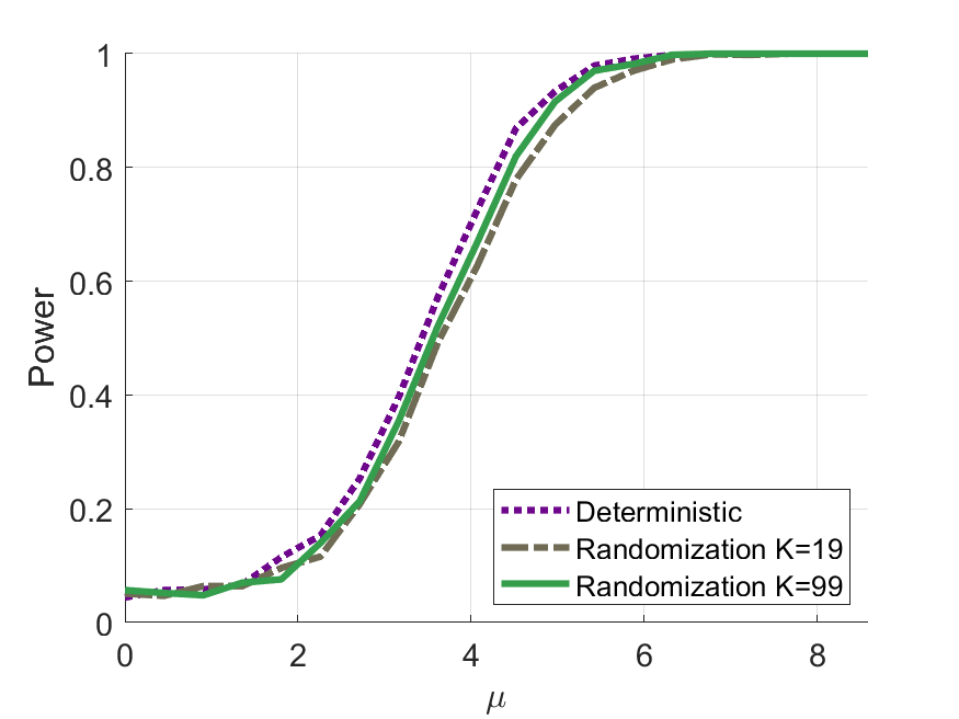
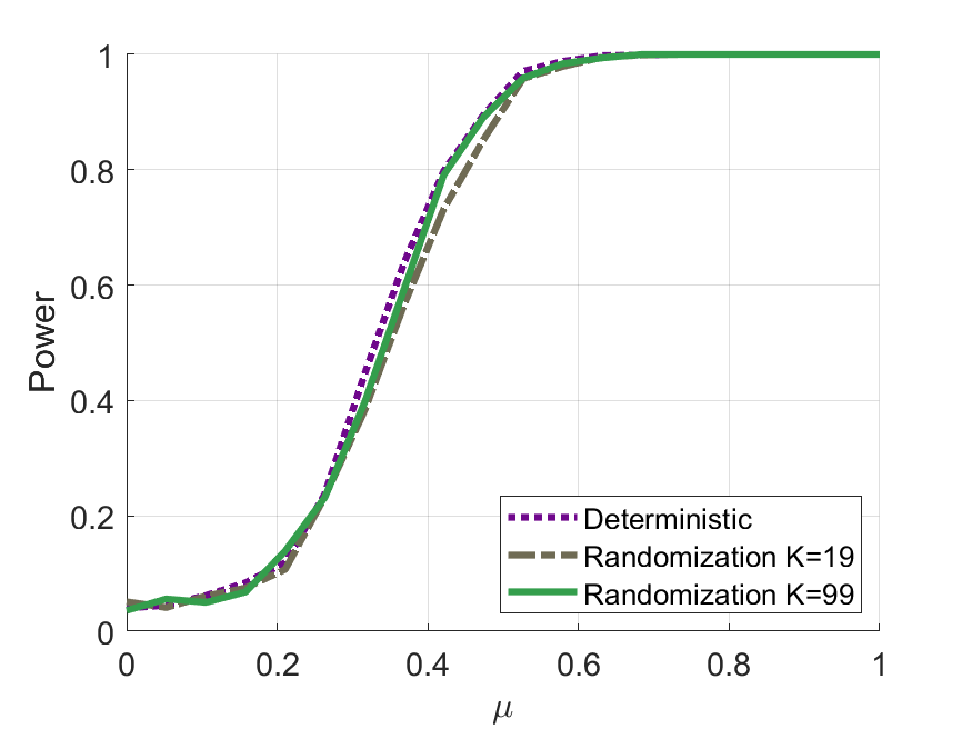
Figure 1: Evaluating the power of the randomization test in comparison with the deterministic test as a function of signal strength in sparse vector detection. Left plot: rotation test; right plot: signflip test. See the text for details.

This condition is a form of relative sparsity: the maximal absolute coordinate $\|s_{m}\|_{\infty}$ is large compared to the $\ell_{2}$ norm $\|s_{m}\|_{2}$ and to the noise level $\|N_{m}\|_{2}$. Proposition 2.2 leads to the condition $\liminf_{m\to\infty}\|s_{m}\|_{\infty}/\|N_{m}\|_{\infty}\geqslant 2$. Now, one can check (and we do in the proof) that $\|N_{m}\|_{\infty}=_{d}\|N_{m}\|_{2}\cdot\|Z_{m}\|_{\infty}/\|Z_{m}\|_{2}$, where $Z_{m}\sim\mathcal{N}(0,I_{p_{m}})$. Moreover, as we also check in the proof, $\|Z_{m}\|_{\infty}\sim(2\log p_{m})^{1/2}$ and $\|Z_{m}\|_{2}\sim p_{m}^{1/2}$. Hence, the condition for the deterministic test is (roughly)

$$\liminf_{m\to\infty}\frac{\|s_{m}\|_{\infty}/(2\log p_{m})^{1/2}}{2t_{m,2}/p_{m}^{1/2}}>1.$$

We can see that the condition is milder that (7) (compare the denominators); but may be asymptotically equivalent if $\|s_{m}\|_{2}=o(t_{m,2})$.

Distribution	Density	Distribution of $\|Z\|^{2}$
Normal	$\sim\exp(-\|z\|_{2}^{2}/2)$	$\chi_{p}^{2}$
Multivar. Cauchy	$\sim(1+\|z\|_{2}^{2})^{-(p+1)/2}$	$p\cdot F_{p,1}$
Multivar. $t$ with $d$ d.o.f.	$\sim(1+\|z\|_{2}^{2}/d)^{-(p+d)/2}$	$p\cdot F_{p,d}$

Table 1: Classical examples of spherical distributions, for random vectors $Z\in\mathbb{R}^{p}$, for $p>0$. The densities are given up to constants independent of the argument $z\in\mathbb{R}^{p}$, and the distribution of $\|Z\|_{2}^{2}$ is given in terms of classical distributions such as the chi-squared distribution with $p$ degrees of freedom ($\chi_{p}^{2}$), and the $F$-distribution with $p$ and $d>0$ degrees of freedom ($F_{p,d}$).

Obtaining consistency results. Therefore, obtaining specific consistency results boils down to controlling $\|N_{m}\|_{2}$, the $\ell_{2}$ norm of a spherically invariant random vector. This distribution can be completely arbitrary. We give a few examples of such random vectors in Table 1, including normal, multivariate $t$, and multivariate Cauchy distributions. See Fang et al. (2018), Chapter 3, for more examples.

1. For $Z_{m}\sim\mathcal{N}(0,I_{p_{m}})$, we have $\|Z_{m}\|_{2}^{2}\sim\chi^{2}_{p_{m}}$. By the chi-squared tail bound in Lemma 8.1 of Birgé (2001), when $\Gamma_{m}\sim\chi^{2}_{p_{m}}$

   $$\mathbb{P}\biggl{(}\Gamma_{m}/p_{m}\geq 1+2\sqrt{\frac{x}{p_{m}}}+\frac{2x}{p_{m}}\biggr{)}\leqslant e^{-x}.$$

   Hence, for any sequence $(l_{m})_{m\geqslant 1}$ such that $l_{m}>0$ for all $m$ and $l_{m}\to\infty$ as $m\to\infty$, $\Gamma_{m}^{1/2}\leqslant p_{m}^{1/2}\left(l_{m}^{1/2}\wedge[1+O((l_{m}/p_{m})^{1/2})]\right)$ with probability tending to unity. Thus we can take $t_{m,2}=p_{m}^{1/2}\left(l_{m}^{1/2}\wedge[1+O((l_{m}/p_{m})^{1/2})]\right)$.

2. For a multivariate Cauchy distribution (and more generally a multivariate $t$ distribution with $d_{m}\geqslant 1$ degrees of freedom), by the chi-squared tail bound in Lemma 8.1 of Birgé (2001), when $\Gamma_{m}\sim\chi^{2}_{d_{m}}$, $\Gamma_{m}/d_{m}\geqslant 1-2\sqrt{x/d_{m}}$ with probability at most $\exp(-x)$. Hence, for any sequence $(l_{m})_{m\geqslant 1}$ such that $l_{m}>0$ for all $m$ and $l_{m}\to\infty$ as $m\to\infty$, $1/\Gamma_{m}^{1/2}\leqslant d_{m}^{1/2}\left(l_{m}^{1/2}\wedge[1+O((l_{m}/d_{m})^{1/4})]\right)$ with probability tending to unity. Thus we can take

   $$t_{m,2}=\frac{p_{m}^{1/2}\left(l_{m}^{1/2}\wedge[1+O((l_{m}/p_{m})^{1/2})]\right)}{d_{m}^{1/2}\left(l_{m}^{1/2}\wedge[1+O((l_{m}/d_{m})^{1/4})]\right)}.$$

Discussion of rate-optimality. In this case, obtaining explicit lower bounds on detection thresholds is much more difficult. We are not aware of any results in this direction under the full level of generality of our model, and thus we discuss the difficulties here. Suppose that the noise distribution has density $p_{m}$ with respect to the Lebesgue measure; since the distribution is rotationally invariant, we have $p_{m}(N_{m})=\pi_{m}(\left\|N_{m}\right\|_{2})$ for some density $\pi_{m}$ on $[0,\infty)$. The chi-squared method shows that to achieve consistency, one must have

$$\lim_{m\to\infty}\int_{x_{m}\in\mathbb{R}^{p_{m}}}\frac{\pi_{m}(\left\|x_{m}-s_{m}\right\|_{2})^{2}}{\pi_{m}(\left\|x_{m}\right\|_{2})}dx_{m}=\infty.$$

For instance, if the noise is distributed as a multivariate $t$ distribution with $d_{m}$ degrees of freedom, with density $c_{m}(1+\|z\|_{2}^{2})^{-(p_{m}+d_{m})/2}$, where $c_{m}=\Gamma[(p_{m}+d_{m})/2]/[\Gamma(d_{m}/2)(\pi d_{m})^{p_{m}/2}]$, then we must show that, with $e_{m}=(p_{m}+d_{m})/2$,

$$\lim_{m\to\infty}c_{m}\int_{x_{m}\in\mathbb{R}^{p_{m}}}\left(\frac{1+\|x_{m}\|_{2}^{2}/d_{m}}{(1+\|x_{m}-s_{m}\|_{2}^{2}/d_{m})^{2}}\right)^{e_{m}}dx_{m}=\infty.$$

By changing variables to $x_{m}-s_{m}$, using the rotational invariance of the density, denoting $\nu_{m}=\|s_{m}\|$, we can express the integral as an expectation with respect to $X_{m}$ distributed as a multivariate $t$ distribution with $d_{m}$ degrees of freedom as

$$\mathbb{E}\left(1+\frac{\nu_{m}(2X_{m,p_{m}}+\nu_{m})}{d_{m}+\|X_{m}\|_{2}^{2}}\right)^{e_{m}}.$$

However, there does not appear to be a simple way to evaluate, or obtain sharp bounds on, this expectation, showing the difficulty of obtaining lower bounds for this problem.

Numerical example. We support our theoretical result by a numerical example. We generate data from the signal-plus-noise model $X_{m}=s_{m}+N_{m}$, where $N_{m}\sim\mathcal{N}(0,I_{p_{m}})$, with $p_{m}=100$ and $s_{m}=(\mu,0,0,\ldots,0)^{\top}$ with the signal strength parameter $\mu$ taking values over a grid of size $20$ spaced equally between 0 and $4\cdot\sqrt{\log p_{m}}$. We evaluate the power of the deterministic test based on $\|X_{m}\|_{\infty}$, tuned to have level equal to $\alpha=0.05$. The critical value $t_{\alpha}$ is set so that $P_{H_{m0}}(\|X_{m}\|_{\infty}\geqslant t_{\alpha})=0.05$, and thus equals $t_{\alpha}=\Phi^{-1}([(1-\alpha)^{1/p_{m}}+1]/2)$, where $\Phi^{-1}$ is the standard normal quantile function, i.e., the inverse of the standard normal cumulative distribution function. In this case, the noise has both rotational and sign symmetry. We also evaluate the power of the randomization test based on $K=19$ and $K=99$ random orthogonal rotations as well as the same number of random signflips, with $\alpha=0.05$. We repeat the experiment 1000 times and plot the average frequency of rejections.

On Figure 1, we observe that, as expected, the randomization tests correctly controls the level (under the null when $\mu=0$). Moreover, the power of all tests increases to unity over the range of signals considered, and the deterministic test has only slightly higher power than the randomization tests. In particular, the randomization tests achieve power almost equal to unity at almost the same point as the deterministic test. This is aligned with our results, and supports our claims that the randomization tests are near-optimal. Further, we also observe that the power with $K=99$ random transforms is slightly higher.

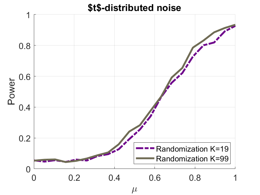
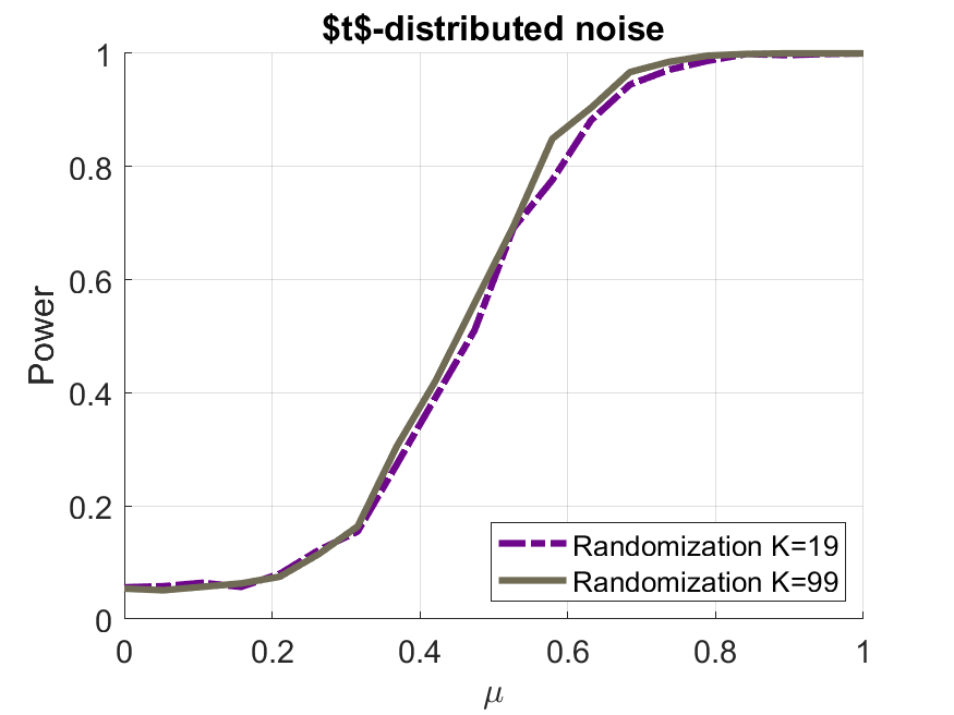
Figure 2: Evaluating the power of the randomization test for $t$-distributed noise. Left plot: $t$ distribution with three degrees of freedom; right plot: $t$ distribution with five degrees of freedom. See the text for details.

Heavy tailed example. One of the the strengths of randomization tests is that they seamlessly apply to heavy tailed noise. To illustrate this, we repeat the above experiment with $t$-distributed noise entries (with three and five degrees of freedom, respectively) instead of normal noise, and using the signflip randomization test. On Figure 2, we observe that the power of the randomization test increases over the range studied; but since the $t$ distribution has heavier tails than the normal, the power increases at a slower rate than in our previous experiment, especially for the $t$ distribution with three degrees of freedom.

3.2 Detecting spikes/low-rank matrices

A second example is the important problem of detecting low-rank matrices, which is fundamental in multivariate statistical analysis, including in PCA and factor analysis, see e.g., Anderson (2003); Muirhead (2009); Johnstone (2001); Dobriban (2020); Johnstone and Onatski (2015); Johnstone and Paul (2018); Hong et al. (2020).

Here the data $X_{m}$ is represented as an $n_{m}\times p_{m}$ matrix, where often $n_{m}$ is the number of samples/datapoints, and $p_{m}$ is the number of features. We are interested to detect if there is a latent signal in the highly noisy observation matrix; and we model this by a matrix with a large operator norm. Formally, $X_{m}=s_{m}+N_{m}$, where $s_{m},N_{m}$ are $n_{m}\times p_{m}$ matrices, and we use the operator norm test statistic $f_{m}(X_{m})=\|X_{m}\|_{\textnormal{op}}=\sigma_{\max}(X_{m})$. This is just one of the many possibilities. One could consider other $\psi$-subadditive test statistics; and in particular norms, such as the maximum absolute entry, $\max_{i,j}|X_{m,ij}|$, or generalized Ky Fan norms of the form $X\mapsto(\sum_{i=1}^{\kappa}\sigma_{i}(X_{m})^{\zeta})^{1/\zeta}$, where $\sigma_{1}(X_{m})\geqslant\ldots\sigma_{n_{m}\wedge p_{m}}(X_{m})\geqslant 0$ are the singular values of $X_{m}$, $\kappa\geqslant 1$, and $\zeta\geqslant 1$ (Li and Tsing, 1988).

As in the previous sections, there are many possible models for the structure of the noise and its corresponding group of invariances. For illustration, we only study one of them here. We consider a model where the columns of $N_{m}$ are independent, and each has a spherical distribution. As in the general theory, we consider a sequence of such signal-plus-noise matrices, for a sequence of signals $s_{m}$. We can then randomize via independent uniform rotations of the columns. Recall that $\|s_{m}\|_{2,\infty}$ is the maximum of the column $\ell_{2}$ norms of $s_{m}$.

Proposition 3.4.

Let the observations follow the matrix signal-plus-noise model $X_{m}=s_{m}+N_{m}$, where $X_{m},s_{m},N_{m}$ are $n_{m}\times p_{m}$-dimensional matrices and each column of $N_{m}$ is independent, with a spherical distribution. As $n_{m},p_{m}\to\infty$ such that $c_{0}\leqslant n_{m}/p_{m}\leqslant c_{1}$ for arbitrary fixed $0<c_{0}<c_{1}$, the sequence of randomization tests (1) with test statistics $\|X_{m}\|_{\textnormal{op}}$ and randomization distributions uniform over the direct product of orthogonal groups $\mathcal{G}_{m}=O(n_{m})\otimes O(n_{m})\ldots\otimes O(n_{m})$ rotating the columns of the data is consistent against the sequence of alternatives with $s_{m}\in\Theta_{m1}$, if there is a sequence $(t_{m,2})_{m\geqslant 1}$ such that with probability tending to unity, $\|N_{m}\|_{2,\infty}\leqslant t_{m,2}$, and for any sequence $(s_{m})_{m\geqslant 1}$ such that for all $m\geqslant 1$, $s_{m}\in\Theta_{m1}$,

$$\liminf_{m\to\infty}\frac{\|s_{m}\|_{\textnormal{op}}/(n_{m}^{1/2}+p_{m}^{1/2})}{(\|s_{m}\|_{2,\infty}+2t_{m,2})/n_{m}^{1/2}}>2.$$

See Section 5.3.3 for the proof. One can verify that Proposition 2.2 implies that the deterministic test based on $\|\hat{\beta}_{m}\|_{\infty}$ is consistent when

$$\liminf_{m\to\infty}\frac{\|s_{m}\|_{\textnormal{op}}/(n_{m}^{1/2}+p_{m}^{1/2})}{2t_{m,2}/n_{m}^{1/2}}>2.$$

When $N_{m}\sim\mathcal{N}(0,I_{n_{m}}\otimes I_{p_{m}})$, one can verify that we can take $t_{m,2}=n_{m}^{1/2}(1+o_{P}(1))$, thus the condition in Proposition 3.4 can be verified to simplify to $\liminf_{m\to\infty}[\|s_{m}\|_{\textnormal{op}}/(n_{m}^{1/2}+p_{m}^{1/2})-\|s_{m}\|_{2,\infty}/n_{m}^{1/2}]>1.$

More generally, suppose that $N_{m}=[\nu_{m,1}O_{m,1};\ldots,\nu_{m,p_{m}}O_{m,p_{m}}]$, where $\nu_{i,m_{i}}$, $i\in[p_{m}]$ are iid from a distribution with cdf $F_{m}$, and $O_{i,m_{i}}$, $i\in[p_{m}]$ are iid according to the Haar measure on the orthogonal group $O(p_{m})$. Then the condition on $t_{m,2}$ is that $P(\max_{i=1}^{p_{m}}\nu_{i,m_{i}}\leqslant t_{m,2})=F_{m}(t_{m,2})^{p_{m}}\to 1$. Consider any sequence $(l_{m})_{m\geqslant 1}$ such that $l_{m}>0$ for all $m$ and $l_{m}\to 0$ as $m\to\infty$. Then, we can take $t_{m,2}=F_{m}^{-1}(1-l_{m}/p_{m})$.

Rate-optimality. Suppose that $N_{m}\sim\mathcal{N}(0,I_{n_{m}}\otimes I_{p_{m}})$, and let $\Theta_{m1}=\{\sqrt{n_{m}/2}\cdot\tau\cdot uv^{\top},v\in\mathbb{R}^{n_{m}},u\in\mathbb{R}^{p_{m}},\|u\|=\|v\|=1\}$. Suppose without loss of generality that $n_{m}\leqslant p_{m}$; otherwise flip the roles of $n_{m}$ and $p_{m}$. Consider a prior $\Pi_{m}$ on $\Theta_{m1}$ such that $u=[v;0_{p_{m}-n_{m}}]$, and $v$ follows a distribution $\Pi_{m}^{\prime}$. Based on (4), we have

$$\textnormal{Var}_{P_{m0}}[L_{m}] =\mathbb{E}_{S,S^{\prime}\sim\Pi_{m}}\exp(S^{\top}S^{\prime})=\mathbb{E}_{uv^{\top},u^{\prime}(v^{\prime})^{\top}\sim\Pi_{m}}\exp(n_{m}\tau^{2}/2\cdot u^{\top}u^{\prime}v^{\top}v^{\prime})$$

$$=\mathbb{E}_{v,v^{\prime}\sim\Pi_{m}^{\prime}}\exp(n_{m}\tau^{2}/2\cdot(v^{\top}v^{\prime})^{2}).$$

This has the exact same form as the expression studied in Theorem 1 of Banks et al. (2018). From that result, it follows that, if $\Pi_{m}^{\prime}$ is uniform over $\{\pm 1\}^{n_{m}}/\sqrt{n_{m}}$ and $\tau<1$, then $\textnormal{Var}_{P_{m0}}[L_{m}]\leqslant C$ for a constant $C<\infty$ not depending on $n_{m}$. This shows a lower bound of order $\tau\gtrsim n_{m}^{1/2}$. Meanwhile, our upper bound simplifies to $\tau\lesssim n_{m}^{1/2}$, showing that randomization tests are rate-optimal in this case.
To summarize:

Proposition 3.5 (Rate-optimality of rotation test for low-rank matrix detection).

Under the assumptions of Proposition 3.4, suppose that $N_{m}\sim\mathcal{N}(0,I_{n_{m}}\otimes I_{p_{m}})$, and let $\Theta_{m1}(\tau_{m})=\{s_{m}=\sqrt{\min(n_{m},p_{m})/2}\cdot\tau_{m}\cdot uv^{\top},v\in\mathbb{R}^{n_{m}},u\in\mathbb{R}^{p_{m}},\|u\|=\|v\|=1\}$. The sequence of rotation tests (1) of the sequence of null hypotheses $s_{m}=0$ from Proposition 3.4 is consistent against the sequence of alternatives with $s_{m}\in\Theta_{m1}(\tau_{m})$ when $\tau_{m}=C\sqrt{\min(n_{m},p_{m})}$ for a sufficiently large constant $C>0$. Moreover, when $\tau_{m}=o(\sqrt{\min(n_{m},p_{m})})$, there is no consistent sequence of tests of $s_{m}=0$ against $s_{m}\in\Theta_{m1}(\tau_{m})$.

3.3 Sparse detection in linear regression

We consider the fundamental linear regression problem $Y_{m}=X_{m}\beta_{m}+\varepsilon_{m}$, where $\varepsilon_{m}$ is random. The null hypothesis is that $\beta_{m}=0$, and we are interested to detect “sparse” alternatives in the same way as in Section 3.1, i.e., vectors $\beta_{m}$ with a large $\ell_{\infty}$ norm.

We can directly view this as a signal plus noise model, where $s_{m}=X_{m}\beta_{m}$. However, the most direct approach of using a test statistic such as $f_{m}(Y_{m})=\|Y_{m}\|_{\infty}$ leads to a condition for consistency that depends on the $\ell_{\infty}$ norm $X_{m}\beta_{m}$ as opposed to $\beta_{m}$ only. Instead, we write the ordinary least squares (OLS) estimator $\hat{\beta}_{m}$ as

$$\hat{\beta}_{m}=X_{m}^{\dagger}Y_{m}=P_{X_{m}}\beta_{m}+X_{m}^{\dagger}\varepsilon_{m},$$

where $X_{m}^{\dagger}$ is the pseudo-inverse of $X_{m}$, and $P_{X_{m}}$ is the projection into the row space of $X_{m}$. Formally, this is the OLS estimator if $n_{m}\geqslant p_{m}$ and $X_{m}$ has full rank; otherwise it is the minimum $\ell_{2}$ norm interpolator of the normal equations $X_{m}^{\top}(Y_{m}-X_{m}\hat{\beta}_{m})=0$. We can view this as a signal-plus-noise model with observation $X^{\prime}_{m}=\hat{\beta}_{m}$, signal $s_{m}=P_{X_{m}}\beta_{m}$, and noise $N_{m}=X_{m}^{\dagger}\varepsilon_{m}$. If $n_{m}\geqslant p_{m}$ and $X_{m}$ has full rank, $s_{m}=\beta_{m}$, but in general this approach only provides information about the projection of $\beta_{m}$ into the row span of $X_{m}$. We are interested to detect sparse signals using the test statistic $f_{m}(\hat{\beta}_{m})=\|\hat{\beta}_{m}\|_{\infty}$.

As before, there are many possibilities for the structure of the noise. As in Section 3.1.1, we consider coordinate-wise sign-symmetric noise, assuming that for any vector $b\in\{\pm 1\}^{n_{m}}$, $(\varepsilon_{m,1},\ldots,\varepsilon_{m,n_{m}})=_{d}(b_{1}\varepsilon_{m,1},\ldots,b_{n_{m}}\varepsilon_{m,n_{m}})$. We consider the randomization test from equation (1), where we randomly flip the sign of the data $Y_{m}$ $K$ times using diagonal matrices $B_{m,i}$, $i=1,\ldots,K$, with iid Rademacher entries on the diagonal. For any $n_{m}$-dimensional vector $v$, define the matrix

$$\mathcal{X}_{m}(v)=[X_{m}^{\dagger}\operatorname{diag}(v);-X_{m}^{\dagger}\operatorname{diag}(v)].$$ (8)

For $j=1,\ldots,p_{m}$, let $[X_{m}^{\dagger}]_{j,\cdot}$ be the $j$-th row of $X_{m}^{\dagger}$. Let

$$T(X_{m})=\{\operatorname{diag}([X_{m}^{\dagger}]_{j,\cdot})X_{m}w:w\in\mathbb{R}^{p_{m}},\|w\|_{\infty}\leqslant 1,j\in[p_{m}]\}.$$ (9)

Define the vector $|\varepsilon_{m}|=(|\varepsilon_{m,1}|,\ldots,|\varepsilon_{m,n_{m}}|)^{\top}$. Recall $U^{+}$ from (5). Below, $\|M\|_{\infty,\infty}=\sup_{\|v\|_{\infty}\leqslant 1}\|Mv\|_{\infty}$ is the induced matrix norm, which is also the maximum of the $\ell_{1}$ norms of the rows of $M$.

Proposition 3.6.

Let the data $(X_{m},Y_{m})$ follow the linear regression model $Y_{m}=X_{m}\beta_{m}+\varepsilon_{m}$, where $Y_{m}$ is an $n_{m}$-dimensional vector of outcomes, $X_{m}$ is and $n_{m}\times p_{m}$-dimensional observation matrix, and $\beta_{m}$ is an unknown $p_{m}$-dimensional vector of regression parameters. Let $\varepsilon_{m}$ have independent entries $\varepsilon_{m,i}$, $i=1,\ldots,n_{m}$, such that $\varepsilon_{m,i}=_{d}-\varepsilon_{m,i}$. The sequence of randomization tests (1) of the null hypothesis $P_{X_{m}}\beta_{m}=0$ with test statistics $\|\hat{\beta}_{m}\|_{\infty}$, where $\hat{\beta}_{m}=X_{m}^{\dagger}Y_{m}$, and randomization distributions uniform over $n_{m}\times n_{m}$ diagonal matrices with independent Bernoulli entries is consistent against the sequence of alternatives with $P_{X_{m}}\beta_{m}\in\Theta_{m1}$, if there are two sequences $(l_{m})_{m\geqslant 1}$ and $(t_{m})_{m\geqslant 1}$ such that the following hold:

1. $l_{m}>0$ for all $m$ and $l_{m}\to\infty$ as $m\to\infty$,

2. $t_{m}>0$ for all $m$ and, with $U^{+}$ from (5) and $\mathcal{X}_{m}$ from (8), $P(U^{+}(\mathcal{X}_{m}(|\varepsilon_{m}|),l_{m})\leqslant t_{m})\to 1$,

3. for any sequence $(P_{X_{m}}\beta_{m})_{m\geqslant 1}$ such that for all $m\geqslant 1$, $P_{X_{m}}\beta_{m}\in\Theta_{m1}$, with $T(X_{m})$ from (9),

   $$\liminf_{m\to\infty}\left(\|P_{X_{m}}\beta_{m}\|_{\infty}\frac{1-U^{+}(T(X_{m}),l_{m})}{2t_{m}}\right)>1.$$

See Section 5.3.4 for the proof. This result bounds the quantity $\|X_{m}^{\dagger}\varepsilon_{m}\|_{\infty}$ by an “asymmetrization” argument first, by conditioning on $|\varepsilon_{m}|$ and using the Bernoulli/Rademacher randomness over the signs of the entries of $\varepsilon_{m}$. However, in specific cases when more is known about the distribution of $\varepsilon_{m}$, one may obtain simpler results by directly bounding this quantity. For instance, when $\varepsilon_{m}\sim\mathcal{N}(0,I_{p_{m}})$, $X_{m}^{\dagger}\varepsilon_{m}\sim\mathcal{N}(0,X_{m}^{\dagger}(X_{m}^{\dagger})^{\top})$, and under certain structural conditions on $X_{m}$, one may be able to derive sharp bounds for the required maximum $\|X_{m}^{\dagger}\varepsilon_{m}\|_{\infty}$ of a correlated multivariate Gaussian random vector.

For comparison, one can verify that Proposition 2.2 implies that the deterministic test based on $\|\hat{\beta}_{m}\|_{\infty}$ is consistent when the (at least as liberal) condition $\liminf_{m\to\infty}\|P_{X_{m}}\beta_{m}\|_{\infty}/(2t_{m})>1$ holds.

Discussion of rate-optimality. There is a large literature on optimal hypothesis testing for linear regression, see for instance Ingster et al. (2010); Arias-Castro et al. (2011); Mukherjee and Sen (2020); Carpentier and Verzelen (2021) and references therein. These works essentially only study iid Gaussian (or sub-Gaussian) noise, and make varying assumptions on the design matrix and signal strength. In general it appears quite difficult to make a direct comparison to our assumptions. For instance the work of Arias-Castro et al. (2011) (their Theorem 2) implies that if $[X_{m}]_{j,\cdot}$ is the $j$-th row of $X_{m}$, and $(c_{m})_{m\geqslant 1}$ is a sequence such that $c_{m}>0$ for all $m$ and $c_{m}\to 0$ as $m\to\infty$, then if $X_{m}^{\top}X_{m}$ is normalized to have unit diagonal entries, if for all $i\in[p_{m}]$, $|\{j\in[p_{m}]:|[X_{m}]_{j,\cdot}^{\top}[X_{m}]_{i,\cdot}|\geqslant c_{m}(\log p_{m})^{-4}\}|=O(p_{m}^{\delta})$ for all $\delta>0$, and if the regression coefficient $\beta_{m}$ can be any 1-sparse vector, then it is required that $\liminf_{m\to\infty}\|\beta_{m}\|_{\infty}/\sqrt{2\log p_{m}}\geqslant 1$ in order for any test to have non-vanishing detection power. The main assumption is that for any feature, the number of other features with correlation above the level $c_{m}(\log p_{m})^{-4}$ is smaller than any positive power of $p_{m}$. This assumption does not appear to be easily comparable to our conditions. Indeed, our conditions require (among others) to bound $\|X_{m}^{\dagger}\varepsilon_{m}\|_{\infty}$, where $X_{m}^{\dagger}\varepsilon_{m}\sim\mathcal{N}(0,X_{m}^{\dagger}(X_{m}^{\dagger})^{\top})$, which does not appear to be directly related to the conditions from Arias-Castro et al. (2011).
Thus, our conditions under which the randomization test works appear to be different from the ones that have been studied before for rate optimality in this problem. Since our main goal in this paper was to develop a general framework that enables proving consistency results for randomization tests, we view it as beyond our scope to fully elucidate the relationships between our conditions and those variously proposed in the literature. We would like to emphasize that our consistency results cover settings where the noise for every observation is assumed to be merely independent and symmetrically distributed, potentially heteroskedastic and heavy-tailed. This goes beyond the settings in which lower bounds have been proved for this problem.

3.4 Two-sample testing

We study a two-sample testing problem, which is a classical and fundamental problem of exceeding importance in statistics, see e.g., (Lehmann and Casella, 1998; Lehmann and Romano, 2005). We study this for illustration purposes only, as there are well-established tests. We do not claim that randomization tests are better, merely that they are applicable, and it is of interest to understand what they lead to.

We consider permutation based randomization tests, valid when the entries of the noise are exchangeable. For a given integer $m\geqslant 1$ and dimension $p_{m}$, let $(f_{\mu})_{\mu\in\mathbb{R}^{p_{m}}}$ be a location family of densities on $\mathbb{R}^{p_{m}}$. Let $\|\cdot\|_{\mathbb{R}^{p_{m}}}$ be a norm on $\mathbb{R}^{p_{m}}$. Let $\varepsilon_{m,i}\sim f_{0_{m}}$ sampled from the location family at the all-zero vector be iid for $i\in[n_{m}]$, and $\varepsilon_{m,i}^{\prime}\sim f_{0_{m}}$ also be iid for $i\in[n_{m}^{\prime}]$.

Proposition 3.7.

Suppose $Z_{m,1},\ldots,Z_{m,n_{m}}\sim f_{\mu_{m}}$, $Y_{m,1},\ldots,Y_{m,n_{m}^{\prime}}\sim f_{\mu_{m}^{\prime}}$ are independent observations, and test the null hypothesis that $\mu_{m}=\mu_{m}^{\prime}$ against the alternative that $\mu_{m}\neq\mu_{m}^{\prime}$. Consider the randomization test (1) with test statistic $\|\bar{Z}_{m}-\bar{Y}_{m^{\prime}}\|_{\mathbb{R}^{p_{m}}}$, where $\bar{Z}_{m}=n_{m}^{-1}\sum_{i=1}^{n_{m}}Z_{m,i}$ and $\bar{Y}_{m}^{\prime}=({n_{m}^{\prime}})^{-1}\sum_{i=1}^{n_{m}^{\prime}}Y_{m,i}$.

For a randomization distribution uniform over the symmetric group of all permutations $S_{n_{m}+n_{m}^{\prime}}$, the sequence of randomization tests (1) of the sequence of null hypotheses $\mu_{m}=\mu_{m}^{\prime}$ is consistent against the sequence of alternatives with $(\mu_{m},\mu_{m}^{\prime})\in\Theta_{m1}$, if

1. as $m\to\infty$, $n_{m}+n_{m}^{\prime}\to\infty$,

2. there is a sequence $(t_{m})_{m\geqslant 1}$ such that $P(\|({n_{m}^{\prime}})^{-1}\sum_{i=1}^{n_{m}^{\prime}}\varepsilon_{m,i}^{\prime}-n_{m}^{-1}\sum_{i=1}^{n_{m}}\varepsilon_{m,i}\|_{\mathbb{R}^{p_{m}}}\leqslant t_{m})\to 1$, where $\varepsilon_{m,i},\varepsilon_{m,j}^{\prime}\sim f_{0_{m}}$, $i\in[n_{m}]$, $j\in[n_{m}^{\prime}]$ are iid.

3. for any sequence $(\mu_{m},\mu_{m}^{\prime})_{m\geqslant 1}$ such that for all $m\geqslant 1$, $(\mu_{m},\mu_{m}^{\prime})\in\Theta_{m1}$,

   $$\liminf_{m\to\infty}\frac{\|\mu_{m}^{\prime}-\mu_{m}\|_{\mathbb{R}^{p_{m}}}}{t_{m}}>2.$$

See Section 5.3.5 for the proof. As for the one-sample test for sparse detection, Proposition 2.2 leads to the same condition; thus suggesting that the additional noise due to randomization is small. The condition looks similar to the one we obtained for the one-sample test; however this concerns a different randomization distribution (permutations), and thus requires a different analysis. Bounding $t_{m}$ depends on the conditions we impose on the location family, on the growth of the dimension and sample sizes, and on the specific norm used. For instance, in certain cases one may use Orlicz-norm based concentration inequalities (see e.g., Section 3.1.1 for examples), which can be adapted to the norm $\|\cdot\|_{\mathbb{R}^{p_{m}}}$.
Following the approach from Section 3.1.1, for $\|\cdot\|_{\mathbb{R}^{p_{m}}}=\|\cdot\|_{\infty}$, the same results stated there apply by assuming the same conditions on the noise vectors for both samples, and by bounding the noise vectors of the two samples separately. For instance, if the entries of $\varepsilon_{m,i}$, $i\in[n_{m}]$, $\varepsilon_{m,i}^{\prime}$, $i\in[n_{m}^{\prime}]$ are iid sub-exponential, then we can take $t_{m}\sim\sqrt{(\log p_{m})/\min(n_{m},n_{m}^{\prime})}$.

Rate-optimality. It is straightforward to see that the lower bound technique from Section 3.1.1 generalizes, and leads to a bound of the order $\tau_{m}=\sqrt{(\log p_{m})/\min(n_{m},n_{m}^{\prime})}$. Indeed, when $n_{m}\leqslant n_{m}^{\prime}$, one can take $\mu_{m^{\prime},j}=0$ and $\mu_{m,j}=\tau_{m}\cdot e_{j}$, for $j\in[n_{m}]$ in the construction of the alternatives in Ingster’s method, and it is straightforward to see that the desired conclusion holds by the same calculation as in Section 3.1.1. This shows that for noise with iid sub-exponential entries, the signflip based randomization test is rate-optimal. To summarize:

Proposition 3.8 (Rate-optimality of permutation test for sparse two-sample testing).

Under the assumptions of Proposition 3.7, suppose that $\varepsilon_{m,i}\sim f_{0_{m}}$ for $i\in[n_{m}]$, and $\varepsilon_{m,i}^{\prime}\sim f_{0_{m}}$ for $i\in[n_{m}^{\prime}]$, have iid entries with a sub-exponential distribution $\pi$. Let $\Theta_{m1}(\tau_{m})=\{(\mu_{m},\mu_{m}^{\prime})\in\mathbb{R}^{p_{m}}\times\mathbb{R}^{p_{m}}:\|\mu_{m}-\mu_{m}^{\prime}\|_{\infty}\geqslant\tau_{m}\}$. The permutation test of the sequence of null hypotheses $\mu_{m}=\mu_{m}^{\prime}$ from Proposition 3.7 is consistent against the sequence of alternatives with $(\mu_{m},\mu_{m}^{\prime})\in\Theta_{m1}(\tau_{m})$ when $\tau_{m}=C\sqrt{\log(p_{m})/\min(n_{m},n_{m}^{\prime})}$ for a sufficiently large constant $C>0$. Moreover, when $\tau_{m}=o(\sqrt{\log(p_{m})/\min(n_{m},n_{m}^{\prime})})$, there is no consistent sequence of tests of $\mu_{m}=\mu_{m}^{\prime}$ against $(\mu_{m},\mu_{m}^{\prime})\in\Theta_{m1}(\tau_{m})$, $m\geqslant 1$.

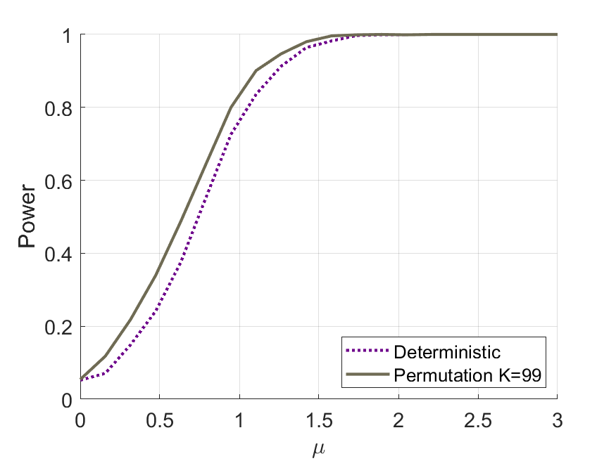
Figure 3: Evaluating the power of a permutation test in comparison with the $t$-test as a function of signal strength in two-sample testing. See the text for details.

Numerical example. We support our theoretical result by a numerical example, using the two-sample $t$-test. We generate data from the Gaussian signal-plus-noise model $Z_{m,i}\sim\mathcal{N}(s_{m},1)$, for $i\in[n_{m}]$, and $Y_{m,i}\sim\mathcal{N}(0,1)$, for $i\in[n_{m}^{\prime}]$, where $s_{m}=\mu$, with the signal strength parameter $\mu$ taking values over a grid of size $20$ spaced equally between 0 and 3. We take $n_{m}=n_{m}^{\prime}=15$. We evaluate the power of the deterministic test based on the two-sample $t$-test, tuned to have level equal to $\alpha=0.05$. We also evaluate the power of the randomization test based on $K=99$ random permutations. We repeat the experiment 1000 times and plot the average frequency of rejections.

On Figure 3, we observe similar phenomena to those mentioned before: the randomization test correctly controls the level, and the power of both tests increases to unity over the range of signals considered. The power of the two tests is very close. In this experiment, the permutation test even has a slightly higher power.

4 Discussion

We developed a set of results on the consistency of randomization tests. While we think that our results are quite powerful, they also have a number of limitations to be addressed in future work:

1. A limitation is the restriction to signal plus noise models. This is needed in the current proof technique; in fact our entire approach is based on this structure. However, to broaden the scope of our results, it would be important to extend to more general statistical models.

2. Another limitation is that the level $\alpha$ is considered fixed. This is also needed in the proof, and is specifically used in the bound (11). In some applications, especially in multiple hypothesis testing, the level $\alpha$ needs to shrink with the problem size. It would be important to extend our theory to this setting.

5 Appendix

5.1 Practical Considerations

When are invariance based tests applicable in practice? When can one invoke the group invariance hypothesis? We think that this is a challenging applied statistics problem, and we provide some discussion here. When a data analyst is performing a hypothesis test, and they have reason to think that under the null hypothesis the distribution of the data is (nearly) unchanged under some operation, then one can invoke a group invariance condition. Suppose for instance that the data analyst thinks that under the null hypothesis, the data is equally likely to have come in any order — then one can invoke permutation invariance. However, suppose that the data comes in predefined clusters (such as strata, or classes based on some key distinguishing class), and under the null hypothesis it is only reasonable to think that that data is equally likely to appear in any order in some specific clusters. Then one can use permutation invariance only over the permutations within those clusters.

This type of reasoning is more readily justifiable when testing a point null. In that case, since we only consider one distribution, assumptions can be justified with greater ease. However if we consider composite null hypotheses, such as those in two-sample testing, then it becomes much more challenging to justify invariance assumptions.

However one difficulty is that formally testing (evaluating) invariance assumptions can be very difficult, especially if the invariance groups are large (for instance suppose that we only have one observation; then it is impossible to test that its density is symmetric around zero). In our view these type of decisions can be quite application-specific. Further there are a number of books and reviews on group invariance and permutation tests in statistics, and the interested statistical data analyst can study them for additional insights (see e.g., Pesarin, 2001; Ernst, 2004; Pesarin and Salmaso, 2010b, 2012; Good, 2006; Kennedy, 1995; Eaton, 1989; Wijsman, 1990; Giri, 1996, etc.).

5.2 Proof for the general theory

5.2.1 Proof of $\psi$-sub-additivity in Section 2.2

Let $x,y\in\mathbb{R}$ and suppose first that $0\leqslant x<y$. Then, by concavity, $c(y)=c(x[x/y]+[x+y][1-x/y])\geqslant c(x)(x/y)+c(x+y)(1-x/y)$, or equivalently, $c(x+y)\leqslant[yc(y)-xc(x)]/[y-x]$. Thus, $c(x+y)\leqslant c(x)+c(y)$ follows if $xc(y)\leqslant yc(x)$. By concavity again, and also using that $c(0)\geqslant 0$, we have $c(x)=c(y[x/y]+0[1-x/y])\geqslant c(y)(x/y)+c(0)(1-x/y)\geqslant c(y)(x/y)$, as required. Next, if $0\leqslant x=y$, then the above argument used for $y=2x$ shows that $c(x)\geqslant c(2x)/2$, thus $c(x+y)=c(2x)\leqslant 2c(x)=c(x)+c(y)$. This finishes the argument when $x,y\geqslant 0$. The same argument applies when $x,y\leqslant 0$.
The remaining case is when $x,y$ have opposite signs. We can assume without loss of generality that $x<0<y$ and that $|y|\geqslant|x|$ (otherwise we can consider $(-x,-y)$). Then $f(x+y)=c(|x+y|)=c(x+y)=c(y-|x|)\leqslant c(y)+c(|x|)$, where the last inequality follows because $c$ is non-decreasing, and also as $0\leqslant c(0)\leqslant c(|x|)$.

5.2.2 Proof of Theorem 2.1

Control of type I error. The first claim, about the level/Type I error control, is discussed at various levels of generality in many works. The textbook result, e.g., Problem 15.3 in Lehmann and Romano (2005) considers finite groups, and for infinite groups (e.g., Problem 15.1 in the same reference), assumes that we average over the full group. See also more general statements in theorem 2 in Hemerik and Goeman (2018b) and theorem 2 in Hemerik and Goeman (2018a). We provide a simple argument to show a key required exchangeability claim, which extends the above results allowing for compact topological groups at a full level of generality, and applies to random sampling of a finite number of group elements. This is crucial for our results, because we use continuous groups such as orthogonal groups in many of our examples.

Let $T_{0}=f_{m}(N_{m})$, and $T_{i}=f_{m}(G_{mi}N_{m})$ for $i=1,\ldots,K$. Note that due to noise invariance, $T_{i}$, $i=0,\ldots,K$ are exchangeable when $N_{m},G_{m1},\ldots,G_{mK}$ are all considered random: the random variables in the vector $L=(N_{m},G_{m1}N_{m},\ldots,G_{mK}N_{m})$ are exchangeable.

Lemma 5.1.

The random vectors $\{N_{m},G_{m1}N_{m},\ldots$, $G_{mK}N_{m}\}$ are mutually exchangeable.

Proof.

To see this, we will show that $L=(N_{m},G_{m1}N_{m},\ldots,G_{mK}N_{m})$ has the same distribution as $B=(G_{m}N_{m},G_{m1}N_{m},\ldots,G_{mK}N_{m})$, where $G_{m}\sim Q_{m}$ is independent of $N_{m},G_{m1},\ldots$, $G_{mK}$. Denote $G_{m}N_{m}=N_{m}^{\prime}$. Then this is equivalent to the statement that $A_{m}$ has the same distribution as $(N_{m}^{\prime},G_{m1}G_{m}^{-1}N_{m}^{\prime},\ldots,G_{mK}G_{m}^{-1}N_{m}^{\prime})$.

Let $G_{mi}^{\prime}=G_{mi}G_{m}^{-1}$, for $i=1,\ldots,K$. Since $N_{m}=_{d}N_{m}^{\prime}$, the above claim follows from because the vectors $(G_{m1},\ldots,G_{mK})$ and $(G_{m1}^{\prime},\ldots,G_{mK}^{\prime})$ have an identical distribution. For simplicity, we show this for $K=2$. The proof for the more general case is very similar.

We can write for $i\neq j$, $Q_{m}(G_{mi}^{\prime}\in M_{i},G_{mj}^{\prime}\in M_{j})=Q_{m}(G_{mi}G_{m}^{-1}\in M_{i},G_{mj}G_{m}^{-1}\in M_{j})=Q_{m}(G_{mi}\in G_{m}M_{i},G_{mj}\in G_{m}M_{j})$. Now, let us condition on $G_{m}$. Then, we can write using the independence of $G_{mi},G_{mj}$ that $Q_{m}(G_{mi}\in G_{m}M_{i},G_{mj}\in G_{m}M_{j}|G_{m})=Q_{m}(G_{mi}\in G_{m}M_{i}|G_{m})Q_{m}(G_{mj}\in G_{m}M_{j}|G_{m})$. Recall that $G_{mi}\sim Q_{m}$ are iid from the Haar/uniform probability measure on $\mathcal{G}_{m}$. Using the left-invariance of the Haar measure, we have $Q_{m}(G_{mi}\in G_{m}M_{i}|G_{m})=Q_{m}(G_{mi}\in M_{i}|G_{m})=Q_{m}(G_{mi}\in M_{i})$, and similarly for $j$. Hence, we find, using again the independence of $G_{mi},G_{mj}$ that

$$Q_{m}(G_{mi}^{\prime}\in M_{i},G_{mj}^{\prime}\in M_{j})=Q_{m}(G_{mi}\in M_{i})Q_{m}(G_{mj}\in M_{j})=Q_{m}(G_{mi}\in M_{i},G_{mj}\in M_{j}).$$

This shows that the joint distribution of $(G_{m1},\ldots,G_{mK})$ and $(G_{m1}^{\prime},\ldots,G_{mK}^{\prime})$ is the same for $K=2$. The same argument works for $K>2$. This finishes the proof. ∎

One can then finish the proof of type I error control as in the proof of theorem 2 in Hemerik and Goeman (2018a).

Consistency. Now we move to the part about consistency. We will consider a slight variant of the invariance-based randomization test, where for a fixed $K\geqslant 1$ we reject the null when

$$f_{m}(X_{m})>\max\left(f_{m}(G_{m1}X_{m}),\ldots,f_{m}(G_{mK}X_{m})\right),$$ (10)

and where each $G_{mi}$, $i=1,\ldots,K$ is chosen uniformly at random over $\mathcal{G}_{m}$. The type I error probability over the random $X_{m}$ and $G_{mi}$ of this test is at most $1/(K+1)$, see Theorem 2.1. The consistency of this test implies the consistency of the quantile-based test. Specifically, given any $\alpha\in(0,1)$, choose any positive integer $K$ such that $1/(K+1)\leqslant\alpha$. Let $R_{m,K}$ denote the event (10) and let $R_{m,\alpha}$ denote the event (1). Then, $R_{m,K}\subset R_{m,\alpha}$, and hence $P_{H_{m1}}(R_{m,K})\leqslant P_{H_{m1}}(R_{m,\alpha})$. We will show that $P_{H_{m1}}(R_{m,K})\to 1$. Thus, it will follow that $P_{H_{m1}}(R_{m,\alpha})\to 1$. Therefore, it is enough to study the test (10). A simplification is given by the following lemma.

Lemma 5.2.

Suppose $K$ is fixed. Then we have $P(f_{m}(X_{m})>\max_{i=1}^{K}f_{m}(G_{mi}X_{m}))\to 1$ if and only if we have $P(f_{m}(X_{m})>f_{m}(G_{m}X_{m}))\to 1$ for a single $G_{m}\sim Q_{m}$.

Proof of Lemma 5.2.

Consider the events $A_{i}=\{f_{m}(X_{m})\leqslant f_{m}(G_{mi}X_{m})\}$. By taking complements, it is enough to show that $P(\cup_{i=1}^{K}A_{i})\to 0$ if and only if $P(A_{1})\to 0$.

Since $G_{mi}$ have the same distribution for all $i\in[k]$, we have $P(A_{i})=P(A_{j})$ for all $i,j$. Moreover, since $A_{1}\subset\cup_{i=1}^{K}A_{i}$, we have by the union bound that

$$P(A_{1})\leqslant P(\cup_{i=1}^{K}A_{i})\leqslant\sum_{i=1}^{K}P(A_{i})=K\cdot P(A_{1}).$$ (11)

Hence, as $K$ is bounded, we have $P(\cup_{i=1}^{K}A_{i})\to 0$ iff $P(A_{1})\to 0$. ∎

Thus, for consistency to hold, it is enough to show that with probability tending to unity,

$$f_{m}(X_{m})>f_{m}(G_{m}X_{m}).$$

Now, $f_{m}(G_{m}X_{m})=f_{m}(G_{m}s_{m}+G_{m}N_{m})$. We have the following:

Lemma 5.3 (Independence Lemma).

If $g_{m}N_{m}=_{d}N_{m}$ for any fixed $g_{m}\in\mathcal{G}_{m}$, then $G_{m}\mathchoice{\mathrel{\hbox to0.0pt{$\displaystyle\perp$\hss}\mkern 2.0mu{\displaystyle\perp}}}{\mathrel{\hbox to0.0pt{$\textstyle\perp$\hss}\mkern 2.0mu{\textstyle\perp}}}{\mathrel{\hbox to0.0pt{$\scriptstyle\perp$\hss}\mkern 2.0mu{\scriptstyle\perp}}}{\mathrel{\hbox to0.0pt{$\scriptscriptstyle\perp$\hss}\mkern 2.0mu{\scriptscriptstyle\perp}}}G_{m}N_{m}$ when $G_{m}\sim Q_{m}$.

Proof of Lemma 5.3.

We can write, for a measurable set $A$

$$P(G_{m}N_{m}\in A|G_{m}=g_{m0}) =P(g_{m0}N_{m}\in A|G_{m}=g_{m0})=P(g_{m0}N_{m}\in A)=P(N_{m}\in A).$$

Since this expression does not depend on $g_{m0}$, the distribution of $G_{m}N_{m}$ does not depend on the value of $G_{m}$; thus $G_{m}N_{m}$ is independent of $G_{m}$. ∎

This implies that for $G_{m},N_{m}$ sampled independently, $G_{m}s_{m}+G_{m}N_{m}$ has the same distribution as $G_{m}s_{m}+N_{m}$. Therefore, $f_{m}(G_{m}X_{m})=_{d}f_{m}(G_{m}s_{m}+N_{m})$, and it is enough to give conditions for the potentially stronger condition that there is a deterministic sequence of critical values $t_{m}^{\prime}$ such that

$$P_{H_{m1}}(f_{m}(G_{m}s_{m}+N_{m})\leqslant t_{m}^{\prime})+P_{H_{m1}}(f_{m}(X_{m})>t_{m}^{\prime})\to 2.$$ (12)

By $\psi$-subadditivity, we can write

$$f_{m}(X_{m})=f_{m}(s_{m}+N_{m}) \geqslant\psi f_{m}(s_{m})-f_{m}(-N_{m}).$$ (13)

Since $t_{m}$ is such that $P(f_{m}(-N_{m})\leqslant t_{m})\to 1$, we conclude that $P(f_{m}(X_{m})\geqslant\psi f_{m}(s_{m})-t_{m})\to 1$. Hence, if $f_{m}(s_{m})>\psi^{-1}[t_{m}^{\prime}(s_{m})+t_{m}],$ then the desired condition $P_{H_{m1}}(f_{m}(X_{m})>t_{m}^{\prime})\to 1$ holds, provided that $P_{H_{m1}}(f_{m}(G_{m}s_{m}+N_{m})\leqslant t_{m}^{\prime})\to 1$. By $\psi$-subadditivity again, we can write

$$f_{m}(G_{m}s_{m}+N_{m}) \leqslant\psi^{-1}[f_{m}(G_{m}s_{m})+f_{m}(N_{m})]\leqslant\psi^{-1}[\tilde{t}_{m}+t_{m}].$$

Taking $t_{m}^{\prime}=\psi^{-1}[\tilde{t}_{m}+t_{m}]$ finishes the proof.

5.2.3 Proof of Proposition 2.2

As in the proof of Theorem 2.1, it is enough to give conditions for the analogue of (12), i.e., that there is a deterministic sequence of critical values $t_{m}^{\prime}$ such that

$$P_{H_{m0}}(f_{m}(N_{m})\leqslant t_{m}^{\prime})+P_{H_{m1}}(f_{m}(X_{m})>t_{m}^{\prime})\to 2.$$

By condition 2(a) of Theorem 2.1, we can take $t_{m}^{\prime}=t_{m}$, and $P_{H_{m0}}(f_{m}(N_{m})\leqslant t_{m}^{\prime})\to 1$. By $\psi$-subadditivity, we have (13). Thus, we only need that $\psi f_{m}(s_{m})-t_{m}>t_{m}$, which is true by (3). This shows that we can take $\tilde{c}_{m}\leqslant t_{m}$ and finishes the proof.

5.3 Proofs for the examples

5.3.1 Proof of Proposition 3.1

Since $\|\cdot\|_{\infty}$ is a norm, it is 1-subadditive. Thus, the condition from Theorem 2.1 reads $n_{m}^{-1}\|1_{n_{m}}^{\top}s_{m}\|_{\infty}>\tilde{t}_{m}(s_{m})+2t_{m}.$ Moreover, $n_{m}^{-1}\|1_{n_{m}}^{\top}s_{m}\|_{\infty}=\|s_{m}\|_{\infty}$. The requirement on $t_{m},\tilde{t}_{m}$ is that with probability tending to unity, $\|n_{m}^{-1}\sum_{i=1}^{n_{m}}N_{m,i}\|_{\infty}\leqslant t_{m}$, and for Rademacher random variables $b_{m,i}$, $i\in[n_{m}]$, with probability tending to unity, $\|n_{m}^{-1}\sum_{i=1}^{n_{m}}b_{m,i}s_{m}\|_{\infty}=|n_{m}^{-1}\sum_{i=1}^{n_{m}}b_{m,i}|\cdot\|s_{m}\|_{\infty}\leqslant\tilde{t}_{m}$.
By Hoeffding’s inequality, for any $C>0$, $P(|n_{m}^{-1}\sum_{i=1}^{n_{m}}b_{m,i}|\geqslant C)\leqslant 2\exp(-2n_{m}C^{2})$. Hence, we can take $\tilde{t}_{m}=(a_{m}/[2n_{m}])^{1/2}\cdot\|s_{m}\|_{\infty}$, for any sequence $(a_{m})_{m\geqslant 1}$ with $a_{m}\to\infty$. Thus, the condition is that for all $m$ large enough,

$$\|s_{m}\|_{\infty}>(a_{m}/[2n_{m}])^{1/2}\cdot\|s_{m}\|_{\infty}+2t_{m}.$$

This requires that $a_{m}/[2n_{m}]<1$, which we can ensure holds for all large enough $n_{m}$ by taking $a_{m}$ to grow sufficiently slowly. For such large $n_{m}$, the condition is

$$\|s_{m}\|_{\infty}>\frac{2t_{m}}{1-(a_{m}/[2n_{m}])^{1/2}}.$$

Clearly, this holds when $a_{m}$ grows sufficiently slowly, for instance when $a_{m}=\log n_{m}$, if $\lim\inf_{m\to\infty}\frac{\|s_{m}\|_{\infty}}{2t_{m}}>1$.

5.3.2 Proof of Proposition 3.3

Since $\|\cdot\|_{\infty}$ is a norm, it is 1-subadditive. Thus, the condition from Theorem 2.1 reads $\|s_{m}\|_{\infty}>\tilde{t}_{m}(s_{m})+2t_{m}.$ The requirement on $t_{m},\tilde{t}_{m}$ is that with probability tending to unity, $\|N_{m}\|_{\infty}\leqslant t_{m}$, and for $O_{m}\sim O(p_{m})$, with probability tending to unity, $\|O_{m}s_{m}\|_{\infty}\leqslant\tilde{t}_{m}$.
Now, for a normal random vector $Z_{m}\sim\mathcal{N}(0,I_{p_{m}})$, we have $\|O_{m}s_{m}\|_{\infty}=_{d}\|Z_{m}\|_{\infty}/\|Z_{m}\|_{2}\cdot\|s_{m}\|_{2}$. For $Z_{m}\sim\mathcal{N}(0,I_{p_{m}})$, using standard chi-squared concentration of measure (Boucheron et al., 2013), we have $\|Z_{m}\|_{2}=p_{m}^{1/2}(1+o_{P}(1))$. Moreover, $\|Z_{m}\|_{\infty}\leqslant(1+o_{P}(1))\sqrt{2\log p_{m}}$ with probability tending to unity. Hence, we can take $\tilde{t}_{m}=(1+o_{P}(1))(2[\log p_{m}]/p_{m})^{1/2}\cdot\|s_{m}\|_{2}$. Similarly, $\|N_{m}\|_{\infty}=\|O_{m}N_{m}\|_{\infty}=_{d}\|Z_{m}\|_{\infty}/\|Z_{m}\|_{2}\cdot\|N_{m}\|_{2}=(1+o_{P}(1))(2[\log p_{m}]/p_{m})^{1/2}\cdot\|N_{m}\|_{2}$.
Thus, the condition is that there is a sequence $t_{m,2}$ such that $P(\|N_{m}\|_{2}\leqslant t_{m,2})\to 1$ and for all $m$ large enough,

$$\|s_{m}\|_{\infty}>(1+o_{P}(1))(2[\log p_{m}]/p_{m})^{1/2}\cdot\left(\|s_{m}\|_{2}+2t_{m,2}\right).$$

This holds when

$$\liminf_{m\to\infty}\frac{\|s_{m}\|_{\infty}/(2\log p_{m})^{1/2}}{\left(\|s_{m}\|_{2}+2t_{m,2}\right)/p_{m}^{1/2}}>1.$$

5.3.3 Proof of Proposition 3.4

Since the maximal singular value is a norm, it is 1-subadditive. Thus, the condition from Theorem 2.1 reads $\|s_{m}\|_{\textnormal{op}}>\tilde{t}_{m}(s_{m})+2t_{m}.$ The requirement on $t_{m},\tilde{t}_{m}$ is that with probability tending to unity, $\|N_{m}\|_{\textnormal{op}}\leqslant t_{m}$, and for $O_{m,1},\ldots,O_{m,p_{m}}\sim O(n_{m})$, with probability tending to unity, $\|[O_{m,1}s_{m,1};\ldots;O_{m,p_{m}}s_{m,p_{m}}]\|_{\textnormal{op}}\leqslant\tilde{t}_{m}$.

Now, for iid normal random vectors $Z_{m,i}\sim\mathcal{N}(0,I_{n_{m}})$, $i\in[p_{m}]$, we have $O_{m,i}s_{m,i}=_{d}Z_{m,i}/\|Z_{m,i}\|_{2}\cdot\|s_{m,i}\|_{2}$. Thus,

$$\|[O_{m,1}s_{m,1};\ldots;O_{m,p_{m}}s_{m,p_{m}}]\|_{\textnormal{op}}=_{d}\|[Z_{m,1}/\|Z_{m,1}\|_{2}\cdot\|s_{m,1}\|_{2};\ldots;Z_{m,p_{m}}/\|Z_{m,p_{m}}\|_{2}\cdot\|s_{m,p_{m}}\|_{2}]\|_{\textnormal{op}}.$$

Further, for any matrix $M=[m_{1};m_{2};\ldots;m_{p_{m}}]$ and scalars $d_{i}$, $i\in[p_{m}]$,

$$\|[d_{1}m_{1};d_{2}m_{2};\ldots;d_{m}m_{p_{m}}]\|_{\textnormal{op}}\leqslant\max_{i}{|d_{i}|}\cdot\|M\|_{\textnormal{op}}.$$

Now, from standard concentration inequalities we have $P(|\|Z_{m,i}\|/n_{m}^{1/2}-1|\geqslant\delta+1/\sqrt{n_{m}})\leqslant 2\exp(-n_{m}\delta^{2}/2)$. This follows from the Lipschitz concentration of Gaussian random variables, see e.g., Example 2.28 in Wainwright (2019), and from the fact that the mean of the $\chi(n_{m})$ random variable $\|Z_{m,i}\|$ is bounded as $\sqrt{n_{m}}-1\leqslant\mathbb{E}\|Z_{m,i}\|\leqslant\sqrt{n_{m}}$, see exercise 3.1 in Boucheron et al. (2013).

Taking a union bound, we find that $P(\max_{i=1,\ldots,p_{m}}|\|Z_{m,i}\|_{2}/n_{m}^{1/2}-1|\geqslant\delta+1/\sqrt{n_{m}})\leqslant 2\exp(\log p_{m}-n_{m}\delta^{2}/2)$. So, $\max_{i=1,\ldots,p_{m}}|\|Z_{m,i}\|_{2}/n_{m}^{1/2}-1|\to_{P}0$ as long as there is a sequence $\delta=\delta_{m}$ such that $\delta_{m}\to 0$ and $n_{m}\delta_{m}^{2}-2\log p_{m}\to\infty$. This holds if $\log p_{m}=o(n_{m})$. Then, we also have that $\max_{i=1,\ldots,p_{m}}|n_{m}^{1/2}/\|Z_{m,i}\|_{2}-1|\to_{P}0$.

Thus denoting $Z_{m}=[Z_{m,1};\ldots;Z_{m,p_{m}}]$, with probability tending to unity,

$$\|[Z_{m,1}/\|Z_{m,1}\|_{2}\cdot\|s_{m,1}\|_{2};\ldots;Z_{m,p_{m}}/\|Z_{m,p_{m}}\|_{2}\cdot\|s_{m,p_{m}}\|_{2}]\|_{\textnormal{op}}\leqslant(1+o_{P}(1))\|s_{m}\|_{2,\infty}/n_{m}^{1/2}\cdot\|Z_{m}\|_{\textnormal{op}}.$$

It is well known that as $n_{m},p_{m}\to\infty$ such that $c_{0}\leqslant n_{m}/p_{m}\leqslant c_{1}$ for some $0<c_{0}<c_{1}$, we have almost surely that $\|Z_{m}\|_{\textnormal{op}}\leqslant(1+o_{P}(1))(\sqrt{n_{m}}+\sqrt{p_{m}})$. This follows from (Davidson and Szarek, 2001, Theorem 2.13). Hence, we can take $\tilde{t}_{m}=(1+o_{P}(1))\|s_{m}\|_{2,\infty}(\sqrt{n_{m}}+\sqrt{p_{m}})/n_{m}^{1/2}$.

Now, due to the distributional invariance of $N_{m}$, we have

$$\|N_{m}\|_{\textnormal{op}}=_{d}\|[Z_{m,1}/\|Z_{m,1}\|_{2}\cdot\|N_{m,1}\|_{2};\ldots;Z_{m,p_{m}}/\|Z_{m,p_{m}}\|_{2}\cdot\|N_{m,p_{m}}\|_{2}]\|_{\textnormal{op}}$$

Hence, using the same argument as above, for any sequence $t_{m,2}$ such that $\|N_{m}\|_{2,\infty}\leqslant t_{m,2}$ with probability tending to unity, we can take $t_{m}=(1+o_{P}(1))(\sqrt{n_{m}}+\sqrt{p_{m}})\cdot t_{m,2}/n_{m}^{1/2}$. Thus, a sufficient condition is that there is a sequence $t_{m,2}$ such that $P(\|N_{m}\|_{2,\infty}\leqslant t_{m,2})\to 1$ and

$$\|s_{m}\|_{\textnormal{op}}>(1+o_{P}(1))[1+(p_{m}/n_{m})^{1/2}]\cdot\left(\|s_{m}\|_{2,\infty}+2t_{m,2}\right).$$

This holds when

$$\liminf_{m\to\infty}\frac{\|s_{m}\|_{\textnormal{op}}/(n_{m}^{1/2}+p_{m}^{1/2})}{(\|s_{m}\|_{2,\infty}+2t_{m,2})/n_{m}^{1/2}}>1.$$

This finishes the proof.

5.3.4 Proof of Proposition 3.6

Since the map $Y_{m}\mapsto\|X_{m}^{\dagger}Y_{m}\|_{\infty}$ is a quasi-norm, it is 1-subadditive. Thus, the condition from Theorem 2.1 reads $\|P_{X_{m}}\beta_{m}\|_{\infty}>\tilde{t}_{m}+2t_{m}.$ The requirement on $t_{m},\tilde{t}_{m}$ is that with probability tending to unity, $\|X_{m}^{\dagger}\varepsilon_{m}\|_{\infty}\leqslant t_{m}$, and for $B_{m}=\operatorname{diag}(b_{m,1},\ldots,b_{m,p_{m}})$ with iid Rademacher entries $b_{m,i}$, $i\in[p_{m}]$, with probability tending to unity, $\|X_{m}^{\dagger}B_{m}X_{m}\beta_{m}\|_{\infty}\leqslant\tilde{t}_{m}$.

Let $(l_{m})_{m\geqslant 1}$ be any sequence such that $l_{m}>0$ for all $m$ and $l_{m}\to\infty$ as $m\to\infty$. Now, conditional on the vector $|\varepsilon_{m}|=(|\varepsilon_{m,1}|,\ldots,|\varepsilon_{m,n_{m}}|)$, $X_{m}^{\dagger}\varepsilon_{m}$ is an $n_{m}$-dimensional Bernoulli process over the rows of the matrix $\mathcal{X}_{m}(|\varepsilon_{m}|).$ Thus, conditional on $|\varepsilon_{m}|$, we have $\|X_{m}^{\dagger}\varepsilon_{m}\|_{\infty}\leqslant$ $U^{+}(\mathcal{X}_{m}(|\varepsilon_{m}|),l_{m})$ with probability going to unity, see (5). Thus, it is enough to take $t_{m}$ to be an upper bound of this quantity with probability tending to unity.

Next, writing $B_{m}=\operatorname{diag}(b_{m})$,

$$\|X_{m}^{\dagger}B_{m}X_{m}\beta_{m}\|_{\infty} \leqslant\|X_{m}^{\dagger}B_{m}X_{m}\|_{\infty,\infty}\cdot\|\beta_{m}\|_{\infty}$$

$$=\max_{j\in[p_{m}]}|[X_{m}^{\dagger}]_{j,\cdot}^{\top}\cdot B_{m}X_{m}\|_{1}\cdot\|\beta_{m}\|_{\infty}$$

$$=\max_{j\in[p_{m}]}\|X_{m}^{\top}\operatorname{diag}([X_{m}^{\dagger}]_{j,\cdot})\cdot b_{m}\|_{1}\cdot\|\beta_{m}\|_{\infty}$$

$$=\|\beta_{m}\|_{\infty}\cdot\sup_{v\in T(X_{m})}v^{\top}b_{m}.$$

Thus, it is enough if $\tilde{t}_{m}=U^{+}(T(X_{m}),l_{m})$. Thus, a sufficient condition is that there is a sequence $(l_{m})_{m\geqslant 1}$ such that $l_{m}>0$ for all $m$ and $l_{m}\to\infty$ as $m\to\infty$, and a sequence $(t_{m})_{m\geqslant 1}$ such that $P(U^{+}(\mathcal{X}_{m}(|\varepsilon_{m}|),l_{m})\leqslant t_{m})\to 1$ and

$$\liminf_{m\to\infty}\|P_{X_{m}}\beta_{m}\|_{\infty}\frac{1-U^{+}(T(X_{m}),l_{m})}{2t_{m}}>1.$$

This finishes the proof.

5.3.5 Proof of Proposition 3.7

We can write $Z_{m,i}=\mu_{m}+\varepsilon_{m,i}$, for $i\in[n_{m}]$, where $\varepsilon_{m,i}\sim f_{0_{m}}$ are iid. Similarly, we can write $Y_{m,i}=\mu_{m}+\varepsilon_{m,i}^{\prime}$, for $i\in[n_{m}^{\prime}]$, where $\varepsilon_{m,i}^{\prime}\sim f_{0_{m}}$ are also iid. We can arrange the datapoints as the rows of a matrix. This model has a signal-plus-noise form with nuisance $\mu_{m,*}=1_{n_{m}+n_{m}^{\prime}}\cdot\mu_{m}^{\top}$ and signal $S=[0_{n_{m}};1_{n_{m}^{\prime}}]\cdot\Delta_{m}^{\top}$, where $\Delta_{m}=\mu_{m}^{\prime}-\mu_{m}$.

We can follow our general approach for problems with nuisance parameters, see Section 2. Let $P_{m}$ be the projection in the orthogonal complement of the span of the nuisance. We project $X_{m}=[Z_{m,1};\ldots;Z_{m,n_{m}};Y_{m,1};\ldots;Y_{m,n_{m}^{\prime}}]$ to $\tilde{X}_{m}=P_{m}X_{m}$, and we obtain a standard signal-plus-noise model $\tilde{X}_{m}=\tilde{s}_{m}+\widetilde{N}_{n}$. Since $P_{m}=I_{n_{m}+n_{m}^{\prime}}-1_{n_{m}+n_{m}^{\prime}}1_{n_{m}+n_{m}^{\prime}}^{\top}/(n_{m}+n_{m}^{\prime})$, we have

$$\tilde{X}_{m}=[I_{n_{m}+n_{m}^{\prime}}-1_{n_{m}+n_{m}^{\prime}}1_{n_{m}+n_{m}^{\prime}}^{\top}/(n_{m}+n_{m}^{\prime})]\tilde{X}_{m}=\tilde{X}_{m}-1_{n_{m}+n_{m}^{\prime}}\bar{X}_{m}^{\top}.$$

Also

$$\tilde{s}_{m}=P_{m}s_{m}=s_{m}-1_{n_{m}+n_{m}^{\prime}}\bar{s}_{m}^{\top}=[-n_{m}^{\prime}\cdot 1_{n_{m}};n_{m}\cdot 1_{n_{m}^{\prime}}]/(n_{m}+n_{m}^{\prime})\cdot\Delta_{m}^{\top}.$$

We can write the test statistic $\|\bar{Y}_{m}-\bar{Z}_{m}\|_{\mathbb{R}^{p_{m}}}$ as $\|w^{\top}\tilde{X}_{m}\|_{\mathbb{R}^{p_{m}}}$, where $w=[-1_{n_{m}}/{n_{m}};1_{n_{m}^{\prime}}/{n_{m}^{\prime}}]$. Note that $P_{m}w=w$.

The test statistic is clearly 1-subadditive. Thus, the condition from Theorem 2.1 reads $\|\Delta_{m}\|_{\mathbb{R}^{p_{m}}}>\tilde{t}_{m}+2t_{m}.$ The requirement on $t_{m},\tilde{t}_{m}$ is that with probability tending to unity, $\|w^{\top}\tilde{N}_{m}\|_{\mathbb{R}^{p_{m}}}\leqslant t_{m}$, and for a uniformly random permutation matrix $\Pi_{m}$ of $n_{m}+n_{m}^{\prime}$ entries, with probability tending to unity, $\|w^{\top}\Pi_{m}\tilde{s}_{m}\|_{\mathbb{R}^{p_{m}}}\leqslant\tilde{t}_{m}$.

Now,

$$\|w^{\top}\tilde{N}_{m}\|_{\mathbb{R}^{p_{m}}}=\|w^{\top}N_{m}\|_{\mathbb{R}^{p_{m}}}=\|\bar{Y}_{m}^{\prime}-\bar{Z}_{m}\|_{\mathbb{R}^{p_{m}}}=\|({n_{m}^{\prime}})^{-1}\sum_{i=1}^{n_{m}^{\prime}}\varepsilon_{m,i}^{\prime}-n_{m}^{-1}\sum_{i=1}^{n_{m}}\varepsilon_{m,i}\|_{\mathbb{R}^{p_{m}}}.$$

Also,

$$\|w^{\top}\Pi_{m}\tilde{s}_{m}\|_{\mathbb{R}^{p_{m}}}=w^{\top}\Pi_{m}w\cdot\frac{n_{m}^{\prime}n_{m}}{n_{m}+n_{m}^{\prime}}\|\Delta_{m}\|_{\mathbb{R}^{p_{m}}}.$$

Consider the random variable $U=w^{\top}\Pi_{m}w$, where the randomness is due to the random permutation matrix $\Pi_{m}$. Let $d=n_{m}+n_{m}^{\prime}$ be the dimension of $w$. Now, if $\pi_{m}:[d]\mapsto[d]$ denotes the permutation represented by $\Pi_{m}$,

$$\mathbb{E}U^{2}=\mathbb{E}w^{\top}\Pi_{m}w\cdot w^{\top}\Pi_{m}w=\mathbb{E}\sum_{ij}w_{i}w_{\pi_{m}(i)}w_{j}w_{\pi_{m}(j)}=\sum_{ij}w_{i}w_{j}\mathbb{E}w_{\pi_{m}(i)}w_{\pi_{m}(j)}.$$

If $i=j$, then $\mathbb{E}w_{\pi_{m}(i)}w_{\pi_{m}(j)}=\mathbb{E}w_{\pi_{m}(i)}^{2}=\|w\|^{2}/d$. If $i\neq j$, then, since $\sum_{k}w_{k}=0$,

$$\mathbb{E}w_{\pi_{m}(i)}w_{\pi_{m}(j)}=\frac{1}{d(d-1)}\sum_{k\neq l}w_{k}w_{l}=-\frac{\|w\|^{2}}{d(d-1)}.$$

Thus,

$$\mathbb{E}U^{2}=\sum_{i}w_{i}^{2}\|w\|^{2}/d+\sum_{i\neq j}w_{i}w_{j}(-\frac{\|w\|^{2}}{d(d-1)})=\|w\|^{4}\left(\frac{1}{d}+\frac{1}{d(d-1)}\right)=\frac{\|w\|^{4}}{d-1}.$$

Now, we can check that $\|w\|^{2}=\frac{n_{m}+n_{m}^{\prime}}{n_{m}^{\prime}n_{m}}$. Therefore, by Chebyshev’s inequality,

$$P(w^{\top}\Pi_{m}w\cdot\frac{n_{m}^{\prime}n_{m}}{n_{m}+n_{m}^{\prime}}\geqslant l_{m})=P(U/\|w\|^{2}\geqslant l_{m})\leqslant\frac{\mathbb{E}(U^{2}/\|w\|^{4})}{l_{m}^{2}}=\frac{1}{(n_{m}+n_{m}^{\prime}-1)l_{m}^{2}}.$$

Thus, if $l_{m}\to\infty$, we can take $\tilde{t}_{m}=l_{m}\cdot\frac{\|\Delta_{m}\|_{\mathbb{R}^{p_{m}}}}{(n_{m}+n_{m}^{\prime}-1)^{1/2}}$. Thus, a sufficient condition is that there is a sequence $(l_{m})_{m\geqslant 1}$ such that $l_{m}>0$ for all $m$ and $l_{m}\to\infty$ as $m\to\infty$, and a sequence $(t_{m})_{m\geqslant 1}$ such that $P(\|({n_{m}^{\prime}})^{-1}\sum_{i=1}^{n_{m}^{\prime}}\varepsilon_{m,i}^{\prime}-n_{m}^{-1}\sum_{i=1}^{n_{m}}\varepsilon_{m,i}\|_{\mathbb{R}^{p_{m}}}\leqslant t_{m})\to 1$ and

$$\|\Delta_{m}\|_{\mathbb{R}^{p_{m}}}>l_{m}\cdot\frac{\|\Delta_{m}\|_{\mathbb{R}^{p_{m}}}}{(n_{m}+n_{m}^{\prime}-1)^{1/2}}+2t_{m}.$$

This requires that $n_{m}+n_{m}^{\prime}\to\infty$. Then, we can take $l_{m}$ to grow sufficiently slowly, and the above condition holds if

$$\liminf_{m\to\infty}\frac{\|\Delta_{m}\|_{\mathbb{R}^{p_{m}}}}{t_{m}}>2.$$

This finishes the proof.

References

- Anderson and Legendre (1999) M. J. Anderson and P. Legendre. An empirical comparison of permutation methods for tests of partial regression coefficients in a linear model. Journal of statistical computation and simulation, 62(3):271–303, 1999.
- Anderson and Robinson (2001) M. J. Anderson and J. Robinson. Permutation tests for linear models. Australian & New Zealand Journal of Statistics, 43(1):75–88, 2001.
- Anderson (2003) T. W. Anderson. An Introduction to Multivariate Statistical Analysis. Wiley New York, 2003.
- Arias-Castro et al. (2011) E. Arias-Castro, E. J. Candès, and Y. Plan. Global testing under sparse alternatives: Anova, multiple comparisons and the higher criticism. The Annals of Statistics, pages 2533–2556, 2011.
- Banks et al. (2018) J. Banks, C. Moore, R. Vershynin, N. Verzelen, and J. Xu. Information-theoretic bounds and phase transitions in clustering, sparse pca, and submatrix localization. IEEE Transactions on Information Theory, 64(7):4872–4894, 2018.
- Barry et al. (2005) W. T. Barry, A. B. Nobel, and F. A. Wright. Significance analysis of functional categories in gene expression studies: a structured permutation approach. Bioinformatics, 21(9):1943–1949, 2005.
- Bednorz and Latała (2013) W. Bednorz and R. Latała. On the suprema of bernoulli processes. Comptes Rendus Mathematique, 351(3-4):131–134, 2013.
- Berry et al. (2014) K. J. Berry, J. E. Johnston, and P. W. Mielke Jr. A chronicle of permutation statistical methods. Springer, 2014.
- Birgé (2001) L. Birgé. An alternative point of view on lepski’s method. in de gunst, m., klaassen, c. and van der vaart, a. eds,. Lecture Notes-Monograph Series 36, pages 113–133, 2001.
- Boucheron et al. (2013) S. Boucheron, G. Lugosi, and P. Massart. Concentration inequalities: A nonasymptotic theory of independence. Oxford university press, 2013.
- Buja and Eyuboglu (1992) A. Buja and N. Eyuboglu. Remarks on parallel analysis. Multivariate behavioral research, 27(4):509–540, 1992.
- Canay et al. (2017) I. A. Canay, J. P. Romano, and A. M. Shaikh. Randomization tests under an approximate symmetry assumption. Econometrica, 85(3):1013–1030, 2017.
- Carpentier and Verzelen (2021) A. Carpentier and N. Verzelen. Optimal sparsity testing in linear regression model. Bernoulli, 27(2):727–750, 2021.
- Catoni (2012) O. Catoni. Challenging the empirical mean and empirical variance: a deviation study. In Annales de l’IHP Probabilités et statistiques, volume 48, pages 1148–1185, 2012.
- Chamakh et al. (2020) L. Chamakh, E. Gobet, and Z. Szabó. Orlicz random fourier features. J. Mach. Learn. Res., 21:145–1, 2020.
- Chamakh et al. (2021) L. Chamakh, E. Gobet, and W. Liu. Orlicz norms and concentration inequalities for -heavy tailed random variables. 2021.
- Chung and Romano (2013) E. Chung and J. P. Romano. Exact and asymptotically robust permutation tests. Annals of Statistics, 41(2):484–507, 2013.
- Churchill and Doerge (1994) G. A. Churchill and R. W. Doerge. Empirical threshold values for quantitative trait mapping. Genetics, 138(3):963–971, 1994.
- David (2008) H. A. David. The beginnings of randomization tests. The American Statistician, 62(1):70–72, 2008.
- Davidson and Szarek (2001) K. R. Davidson and S. J. Szarek. Local operator theory, random matrices and banach spaces. Handbook of the geometry of Banach spaces, 1(317-366):131, 2001.
- Diaconis (1988) P. Diaconis. Group representations in probability and statistics. Lecture Notes-Monograph Series, 11:1–192, 1988.
- Dobriban (2020) E. Dobriban. Permutation methods for factor analysis and pca. The Annals of Statistics, 48(5):2824–2847, 2020.
- Dobriban and Owen (2019) E. Dobriban and A. B. Owen. Deterministic parallel analysis: an improved method for selecting factors and principal components. Journal of the Royal Statistical Society: Series B (Statistical Methodology), 81(1):163–183, 2019.
- Dwass (1957) M. Dwass. Modified randomization tests for nonparametric hypotheses. The Annals of Mathematical Statistics, pages 181–187, 1957.
- Eaton (1989) M. L. Eaton. Group invariance applications in statistics. In Regional conference series in Probability and Statistics, 1989.
- Eden and Yates (1933) T. Eden and F. Yates. On the validity of fisher’s z test when applied to an actual example of non-normal data. The Journal of Agricultural Science, 23(1):6–17, 1933.
- Efron and Tibshirani (2007) B. Efron and R. Tibshirani. On testing the significance of sets of genes. The annals of applied statistics, 1(1):107–129, 2007.
- Eklund et al. (2016) A. Eklund, T. E. Nichols, and H. Knutsson. Cluster failure: Why fMRI inferences for spatial extent have inflated false-positive rates. Proceedings of the National Academy of Sciences, 113(28):7900–7905, 2016.
- Epstein et al. (2012) M. P. Epstein, R. Duncan, Y. Jiang, K. N. Conneely, A. S. Allen, and G. A. Satten. A permutation procedure to correct for confounders in case-control studies, including tests of rare variation. The American Journal of Human Genetics, 91(2):215–223, 2012.
- Ernst (2004) M. D. Ernst. Permutation methods: a basis for exact inference. Statistical Science, 19(4):676–685, 2004.
- Fang et al. (2018) K.-T. Fang, S. Kotz, and K. W. Ng. Symmetric multivariate and related distributions. Chapman and Hall/CRC, 2018.
- Fisher (1935) R. A. Fisher. The design of experiments. Oliver and Boyd, 1935.
- Folland (2016) G. B. Folland. A course in abstract harmonic analysis, volume 29. CRC press, 2016.
- Freedman and Lane (1983) D. Freedman and D. Lane. A nonstochastic interpretation of reported significance levels. Journal of Business & Economic Statistics, 1(4):292–298, 1983.
- Fulton and Harris (2013) W. Fulton and J. Harris. Representation theory: a first course, volume 129. Springer Science & Business Media, 2013.
- Ganong and Jäger (2018) P. Ganong and S. Jäger. A permutation test for the regression kink design. Journal of the American Statistical Association, 113(522):494–504, 2018.
- Giri (1996) N. C. Giri. Group invariance in statistical inference. World Scientific, 1996.
- Good (2006) P. I. Good. Permutation, parametric, and bootstrap tests of hypotheses. Springer Science & Business Media, 2006.
- Gupta and Varga (2012) A. K. Gupta and T. Varga. Elliptically contoured models in statistics, volume 240. Springer Science & Business Media, 2012.
- Hall (2015) B. Hall. Lie groups, Lie algebras, and representations: an elementary introduction, volume 222. Springer, 2015.
- Hemerik and Goeman (2018a) J. Hemerik and J. Goeman. Exact testing with random permutations. Test, 27(4):811–825, 2018a.
- Hemerik and Goeman (2018b) J. Hemerik and J. J. Goeman. False discovery proportion estimation by permutations: confidence for significance analysis of microarrays. Journal of the Royal Statistical Society: Series B (Statistical Methodology), 80(1):137–155, 2018b.
- Hemerik and Goeman (2020) J. Hemerik and J. J. Goeman. Another look at the lady tasting tea and differences between permutation tests and randomisation tests. International Statistical Review, 2020.
- Hemerik et al. (2019) J. Hemerik, A. Solari, and J. J. Goeman. Permutation-based simultaneous confidence bounds for the false discovery proportion. Biometrika, 106(3):635–649, 2019.
- Hemerik et al. (2020a) J. Hemerik, J. J. Goeman, and L. Finos. Robust testing in generalized linear models by sign flipping score contributions. Journal of the Royal Statistical Society: Series B (Statistical Methodology), 82(3):841–864, 2020a.
- Hemerik et al. (2020b) J. Hemerik, M. Thoresen, and L. Finos. Permutation testing in high-dimensional linear models: an empirical investigation. Journal of Statistical Computation and Simulation, pages 1–18, 2020b.
- Hoeffding (1952) W. Hoeffding. The large-sample power of tests based on permutations of observations. The Annals of Mathematical Statistics, pages 169–192, 1952.
- Hong et al. (2020) D. Hong, Y. Sheng, and E. Dobriban. Selecting the number of components in pca via random signflips. arXiv preprint arXiv:2012.02985, 2020.
- Horn (1965) J. L. Horn. A rationale and test for the number of factors in factor analysis. Psychometrika, 30(2):179–185, June 1965. doi: 10.1007/bf02289447.
- Ingster (1987) Y. I. Ingster. Minimax testing of nonparametric hypotheses on a distribution density in the metrics. Theory of Probability & Its Applications, 31(2):333–337, 1987.
- Ingster and Suslina (2012) Y. Ingster and I. A. Suslina. Nonparametric goodness-of-fit testing under Gaussian models, volume 169. Springer Science & Business Media, 2012.
- Ingster et al. (2010) Y. I. Ingster, A. B. Tsybakov, and N. Verzelen. Detection boundary in sparse regression. Electronic Journal of Statistics, 4:1476–1526, 2010.
- James and Liebeck (2001) G. James and M. Liebeck. Representations and characters of groups. Cambridge University Press, 2001.
- Janssen and Pauls (2003) A. Janssen and T. Pauls. How do bootstrap and permutation tests work? Annals of statistics, 31(3):768–806, 2003.
- Jentsch and Pauly (2015) C. Jentsch and M. Pauly. Testing equality of spectral densities using randomization techniques. Bernoulli, 21(2):697–739, 2015.
- Johnstone (2001) I. M. Johnstone. On the distribution of the largest eigenvalue in principal components analysis. Annals of Statistics, 29(2):295–327, 2001.
- Johnstone and Onatski (2015) I. M. Johnstone and A. Onatski. Testing in high-dimensional spiked models. arXiv preprint arXiv:1509.07269, 2015.
- Johnstone and Paul (2018) I. M. Johnstone and D. Paul. Pca in high dimensions: An orientation. Proceedings of the IEEE, 106(8):1277–1292, 2018.
- Kai-Tai and Yao-Ting (1990) F. Kai-Tai and Z. Yao-Ting. Generalized multivariate analysis. Science Press Beijing and Springer-Verlag, Berlin, 1990.
- Kallenberg (2006) O. Kallenberg. Probabilistic symmetries and invariance principles. Springer Science & Business Media, 2006.
- Kennedy (1995) F. E. Kennedy. Randomization tests in econometrics. Journal of Business & Economic Statistics, 13(1):85–94, 1995.
- Kim et al. (2020a) I. Kim, S. Balakrishnan, and L. Wasserman. Minimax optimality of permutation tests. arXiv preprint arXiv:2003.13208, 2020a.
- Kim et al. (2020b) I. Kim, S. Balakrishnan, and L. Wasserman. Robust multivariate nonparametric tests via projection averaging. Annals of Statistics, 48(6):3417–3441, 2020b.
- Knapp (2013) A. W. Knapp. Lie groups beyond an introduction, volume 140. Springer Science & Business Media, 2013.
- Langsrud (2005) O. Langsrud. Rotation tests. Statistics and computing, 15(1):53–60, 2005.
- Lehmann and Casella (1998) E. Lehmann and G. Casella. Theory of point estimation. Springer Texts in Statistics, 1998.
- Lehmann and Stein (1949) E. L. Lehmann and C. Stein. On the theory of some non-parametric hypotheses. The Annals of Mathematical Statistics, 20(1):28–45, 1949.
- Lehmann (2012) E. L. Lehmann. Parametric versus nonparametrics: two alternative methodologies. In Selected works of EL Lehmann, pages 437–445. Springer, 2012.
- Lehmann and Romano (2005) E. L. Lehmann and J. P. Romano. Testing statistical hypotheses. Springer Science & Business Media, 2005.
- Li and Tsing (1988) C.-K. Li and N.-K. Tsing. Some isometries of rectangular complex matrices. Linear and Multilinear Algebra, 23(1):47–53, 1988.
- Lugosi and Mendelson (2019) G. Lugosi and S. Mendelson. Mean estimation and regression under heavy-tailed distributions: A survey. Foundations of Computational Mathematics, 19(5):1145–1190, 2019.
- Lugosi and Mendelson (2021) G. Lugosi and S. Mendelson. Robust multivariate mean estimation: the optimality of trimmed mean. The Annals of Statistics, 49(1):393–410, 2021.
- Marchina (2019) A. Marchina. About the rate function in concentration inequalities for suprema of bounded empirical processes. Stochastic processes and their applications, 129(10):3967–3980, 2019.
- Muirhead (2009) R. J. Muirhead. Aspects of multivariate statistical theory, volume 197. John Wiley & Sons, 2009.
- Mukherjee and Sen (2020) R. Mukherjee and S. Sen. On minimax exponents of sparse testing. arXiv preprint arXiv:2003.00570, 2020.
- Narici and Beckenstein (2010) L. Narici and E. Beckenstein. Topological vector spaces. CRC Press, 2010.
- Onghena (2018) P. Onghena. Randomization tests or permutation tests? a historical and terminological clarification. Randomization, masking, and allocation concealment, pages 209–228, 2018.
- Pauly et al. (2015) M. Pauly, E. Brunner, and F. Konietschke. Asymptotic permutation tests in general factorial designs. Journal of the Royal Statistical Society: Series B: Statistical Methodology, pages 461–473, 2015.
- Peres-Neto et al. (2005) P. R. Peres-Neto, D. A. Jackson, and K. M. Somers. How many principal components? stopping rules for determining the number of non-trivial axes revisited. Computational Statistics & Data Analysis, 49(4):974–997, 2005.
- Perry and Owen (2010) P. O. Perry and A. B. Owen. A rotation test to verify latent structure. Journal of Machine Learning Research, 11(2), 2010.
- Pesarin and Salmaso (2013) F. Pesarin and L. Salmaso. On the weak consistency of permutation tests. Communications in Statistics-Simulation and Computation, 42(6):1368–1379, 2013.
- Pesarin (1990) F. Pesarin. On a nonparametric combination method for dependent permutation tests with applications. Psychotherapy and Psychosomatics, 54(2-3):172–179, 1990.
- Pesarin (2001) F. Pesarin. Multivariate permutation tests: with applications in biostatistics. Wiley Chichester, 2001.
- Pesarin (2015) F. Pesarin. Some elementary theory of permutation tests. Communications in Statistics-Theory and Methods, 44(22):4880–4892, 2015.
- Pesarin and Salmaso (2010a) F. Pesarin and L. Salmaso. Finite-sample consistency of combination-based permutation tests with application to repeated measures designs. Journal of Nonparametric Statistics, 22(5):669–684, 2010a.
- Pesarin and Salmaso (2010b) F. Pesarin and L. Salmaso. Permutation tests for complex data: theory, applications and software. John Wiley & Sons, 2010b.
- Pesarin and Salmaso (2012) F. Pesarin and L. Salmaso. A review and some new results on permutation testing for multivariate problems. Statistics and Computing, 22(2):639–646, 2012.
- Petrov (2012) V. Petrov. Sums of independent random variables, volume 82. Springer Science & Business Media, 2012.
- Pitman (1937a) E. J. G. Pitman. Significance tests which may be applied to samples from any populations. ii. the correlation coefficient test. Supplement to the Journal of the Royal Statistical Society, 4(2):225–232, 1937a.
- Pitman (1937b) E. J. Pitman. Significance tests which may be applied to samples from any populations. Supplement to the Journal of the Royal Statistical Society, 4(1):119–130, 1937b.
- Pitman (1939) E. Pitman. Tests of hypotheses concerning location and scale parameters. Biometrika, 31(1/2):200–215, 1939.
- Polyanskiy (2019) Y. Polyanskiy. Information theoretic methods in statistics and computer science: f-divergences. URL http://people.lids.mit.edu/yp/homepage/data/LN_fdiv.pdf. 2019.
- Purcell et al. (2007) S. Purcell, B. Neale, K. Todd-Brown, L. Thomas, M. A. Ferreira, D. Bender, J. Maller, P. Sklar, P. I. De Bakker, M. J. Daly, et al. Plink: a tool set for whole-genome association and population-based linkage analyses. The American journal of human genetics, 81(3):559–575, 2007.
- Rao et al. (2019) K. Rao, R. Drikvandi, and B. Saville. Permutation and bayesian tests for testing random effects in linear mixed-effects models. Statistics in medicine, 38(25):5034–5047, 2019.
- Rio (2017) E. Rio. About the constants in the fuk-nagaev inequalities. Electronic Communications in Probability, 22:1–12, 2017.
- Romano (1989) J. P. Romano. Bootstrap and randomization tests of some nonparametric hypotheses. The Annals of Statistics, pages 141–159, 1989.
- Romano (1990) J. P. Romano. On the behavior of randomization tests without a group invariance assumption. Journal of the American Statistical Association, 85(411):686–692, 1990.
- Salimi-Khorshidi et al. (2011) G. Salimi-Khorshidi, S. M. Smith, and T. E. Nichols. Adjusting the effect of nonstationarity in cluster-based and tfce inference. Neuroimage, 54(3):2006–2019, 2011.
- Serre (1977) J.-P. Serre. Linear representations of finite groups, volume 42. Springer, 1977.
- Simpson et al. (2013) S. L. Simpson, R. G. Lyday, S. Hayasaka, A. P. Marsh, and P. J. Laurienti. A permutation testing framework to compare groups of brain networks. Frontiers in computational neuroscience, 7:171, 2013.
- Solari et al. (2014) A. Solari, L. Finos, and J. J. Goeman. Rotation-based multiple testing in the multivariate linear model. Biometrics, 70(4):954–961, 2014.
- Southworth et al. (2009) L. K. Southworth, S. K. Kim, and A. B. Owen. Properties of balanced permutations. Journal of Computational Biology, 16(4):625–638, 2009.
- Subramanian et al. (2005) A. Subramanian, P. Tamayo, V. K. Mootha, S. Mukherjee, B. L. Ebert, M. A. Gillette, A. Paulovich, S. L. Pomeroy, T. R. Golub, E. S. Lander, et al. Gene set enrichment analysis: a knowledge-based approach for interpreting genome-wide expression profiles. Proceedings of the National Academy of Sciences, 102(43):15545–15550, 2005.
- Talagrand (2014) M. Talagrand. Upper and lower bounds for stochastic processes: modern methods and classical problems, volume 60. Springer Science & Business Media, 2014.
- Toulis (2019) P. Toulis. Life after bootstrap: Residual randomization inference in regression models. arXiv preprint arXiv:1908.04218, 2019.
- Tusher et al. (2001) V. G. Tusher, R. Tibshirani, and G. Chu. Significance analysis of microarrays applied to the ionizing radiation response. Proceedings of the National Academy of Sciences, 98(9):5116–5121, 2001.
- van de Geer and Lederer (2013) S. van de Geer and J. Lederer. The bernstein–orlicz norm and deviation inequalities. Probability theory and related fields, 157(1-2):225–250, 2013.
- Vershynin (2018) R. Vershynin. High-Dimensional Probability. Cambridge University Press, 2018.
- Wainwright (2019) M. J. Wainwright. High-Dimensional Statistics: A Non-Asymptotic Viewpoint. Cambridge Series in Statistical and Probabilistic Mathematics. Cambridge University Press, 2019. doi: 10.1017/9781108627771.
- Wedderburn (1975) R. Wedderburn. Random rotations and multivariate normal simulation. Research Report, Rothamsted Experimental Station, 1975. URL https://www.langsrud.com/stat/wedderburn.doc.
- Welch (1990) W. J. Welch. Construction of permutation tests. Journal of the American Statistical Association, 85(411):693–698, 1990.
- Wijsman (1990) R. A. Wijsman. Invariant measures on groups and their use in statistics. IMS, 1990.
- Winkler et al. (2014) A. M. Winkler, G. R. Ridgway, M. A. Webster, S. M. Smith, and T. E. Nichols. Permutation inference for the general linear model. Neuroimage, 92:381–397, 2014.