Triangulation and Persistence: Algebra 101

Abstract.

This paper lays the foundations of triangulated persistence categories (TPC), which brings together persistence modules with the theory of triangulated categories. As a result we introduce several measurements and metrics on the set of objects of some triangulated categories. We also provide examples of TPC’s coming from algebra, algebraic topology, microlocal sheaf theory and symplectic topology.

1. Introduction

Persistence theory, invented for the first time in Zomorodian-Carlsson’s pioneering work [48], is an abstract framework that emerged from investigations in parts of machine learning as well as algebraic and differential topology formalizing the structure and properties of a class of phenomena that are most easily seen in the homology of a filtered chain complex over a field $\mathbf{k}$, $\ldots\subset(C^{\leq\alpha},d)\subset(C^{\leq\beta},d)\subset\ldots\subset(C,d)$ (for $\alpha<\beta,\alpha,\beta\in\mathbb{R}$). The homology of such a complex forms a family $\{H(C^{\leq\alpha})\}_{\alpha\in\mathbb{R}}$ related by maps $i_{\alpha,\beta}:H(C^{\leq\alpha})\to H(C^{\leq\beta})$, $\alpha\leq\beta$ subject to obvious compatibilities and called a persistence module. Given two filtered complexes $(C,d)$ and $(D,d)$ that are quasi-isomorphic, it is possible to compare them by the so-called bottleneck distance. Its definition is based on the fact that the linear maps $v:C\to D$ are themselves filtered by their “shift”: $v$ is of shift $\leq r$ if $v(C^{\leq\alpha})\subset D^{\leq\alpha+r}$, for all $\alpha\in\mathbb{R}$. Using this, given two chain maps $\phi:C\to D$, $\psi:D\to C$ such that $\psi\circ\phi\simeq id_{C}$, there is a natural measurement for how far the composition $\psi\circ\phi$ is from the identity, namely the infimum of the “shifts” of chain homotopies $h:C\to C$ such that $dh+hd=\psi\circ\phi-id$. The machinery of persistence modules is much more developed than the few elements mentioned here. For a survey on this topic and its applications in various mathematical branches, see research monographs from Edelsbrunner [21], Chazal-de Silva-Glisse-Oudot [12], and Polterovich-Rosen-Samvelyan-Zhang [35]. In particular, there is a beautiful interpretation of the bottleneck distance in terms of so-called barcodes ([3], [44]), but we can already formulate the question that we address in this paper.

How can one use a persistence type structure on the morphisms of some (small) category to compare not only (quasi)-isomorphic objects but rather define a pseudo-metric on the set of all objects ?

We provide here a solution to this question based on mixing persistence with triangulation. Triangulated categories are basic algebraic structures with applications in algebraic geometry, algebraic and symplectic topology, mathematical physics and other fields. They were introduced independently by Puppe [36] and Verdier [45] in the early ’60’s. A triangulated category $\mathcal{D}$ is a category endowed with a translation endomorphism $T$ and a class of so called “distinguished (or exact) triangles” - meaning a triple of objects and morphisms $A\to B\to C\to TA$ - subject to four axioms. These axioms mimic abstractly the properties of cone attachments in topology, where the object $C$ is obtained by attaching a cone over a continuous map $A\to B$. For instance, one axiom claims that any morphism can be included in a distinguished triangle (corresponding to the fact that one can attach a cone over any continuous map) and another, the octahedral axiom, can be viewed as a form of associativity for cone attachments.

Given a triangulated category $\mathcal{D}$ there is a simple notion of triangular weight $w$ on $\mathcal{D}$ that we introduce in §2. This associates to each distinguished triangle $\Delta$ a non-negative number $w(\Delta)$ satisfying a couple of properties. The most relevant of them is a weighted variant of the octahedral axiom (we will give a more precise definition later). A basic example of a triangular weight is the flat one: it associates to each distinguished triangle the value $1$. The interest of triangular weights is that they naturally lead to fragmentation pseudo-metrics on $\mathrm{Obj}(\mathcal{D})$ (we assume here that $\mathcal{D}$ is small) defined roughly as follows (see §2 for details). Such a pseudo-metric depends on a family of objects $\mathcal{F}$ of $\mathcal{D}$. With $\mathcal{F}$ fixed, and up to a certain normalization, the pseudo-distance $d^{\mathcal{F}}(X,Y)$ between $X$, $Y\in\mathrm{Obj}(\mathcal{D}))$ is (the symmetrization of) the infimum of the total weight of distinguished triangles needed to construct iteratively $X$ out of $Y$ by only attaching cones over morphisms with domain in $\mathcal{F}$. The weighted octahedral axiom implies that this $d^{\mathcal{F}}$ satisfies the triangle inequality. Using such pseudo-metrics one can analyze rigidity properties of various categories by exploring the induced topology on $\mathrm{Obj}(\mathcal{D})$, in particular, by identifying cases when relevant fragmentation pseudo-metrics are non-degenerate. One can also study the dynamical properties of endofunctors $\phi$ of $\mathcal{D}$ by estimating $d^{\mathcal{F}}(X,\phi^{k}(X))$ for $X\in\mathrm{Obj}(\mathcal{D})$ as well as various associated asymptotic invariants.

Even the fragmentation pseudo-metrics associated to the flat weight are of interest. Many qualitative questions concerned with numerical lower bounds for the complexity of certain geometric objects - classical examples are the Morse inequalities, the Lusternik-Schnirelmann inequality as well as, in symplectic topology, the inequalities predicted by the Arnold conjectures - can be understood by means of inequalities involving such fragmentation pseudo-metrics. Remarkable results based on measurements using this flat weight and applied to the study of endofunctors have appeared recently in work of Orlov [34] as well as Dimitrov-Haiden-Katzarkov-Kontsevich [19] and Fan-Filip [22]. On the other hand, a discrete weight, such as the flat one, is not ideal in a variety of geometric contexts because the associated fragmentation pseudo-metrics vanish on too many pairs of objects.

The main aim of the paper is to show how to use persistence machinery to produce “exotic” (non-flat) triangular weights and associated fragmentation pseudo-metrics. The main tool is a type of refinement of triangulated categories, called Triangulated Persistence Categories (TPC). A triangulated persistence category, $\mathcal{C}$, has two main properties. First, it is a persistence category, a natural notion we introduce in §3. This is a category $\mathcal{C}$ whose morphisms ${\rm Mor}_{\mathcal{C}}(A,B)$ are persistence modules, $\{\{{\rm Mor}^{r}_{\mathcal{C}}(A,B)\}_{r\in\mathbb{R}}\},\{i_{r,s}\}_{r\leq s}\}$ (see [35] for a general introduction of the persistence module theory), and that satisfies obvious relations relative to composition. The second main structural property of TPC’s is that the objects of $\mathcal{C}$ together with the “shift” $0$ morphisms ${\rm Mor}^{0}_{\mathcal{C}}(A,B)$ have the structure of a triangulated category. The formal definition of TPC’s is given in §4. The mixture of the persistence and triangulation structures gives rise to a rich algebraic framework. In particular, we will show how to endow such a $\mathcal{C}$ with a class of weighted triangles. The main result of the paper, in Theorem 5.1.2, shows that the properties of these weighted triangles lead to a triangulated structure on the limit category $\mathcal{C}_{\infty}$ - that has the same objects as $\mathcal{C}$ and has as morphisms the $\infty$-limits of the morphisms in $\mathcal{C}$ - as well as to a triangular weight on $\mathcal{C}_{\infty}$.

Therefore, if a triangulated category $\mathcal{D}$ admits a TPC refinement - that is a TPC, $\mathcal{C}$, such that $\mathcal{C}_{\infty}=\mathcal{D}$ (as triangulated categories), then $\mathcal{D}$ carries an exotic triangular weight induced from the persistence structure of $\mathcal{C}$. As a result, this construction provides a technique to build non-discrete fragmentation pseudo-metrics on the objects of $\mathcal{D}$. The construction of TPC’s is inspired by recent constructions in symplectic topology and, in particular, by the shadow pseudo-metrics introduced in [8] and [5] in the study of Lagrangian cobordism. Remarkably, in that case, rigidity in the sense of the non-degeneracy of the fragmentation metrics is implied by symplectic rigidity in the sense of unobstructedness and, conversely, flexibility in the sense of Gromov’s h-principle, implies that the relevant fragmentation pseudo-metrics vanish. However, the general set-up of TPC’s is independent of symplectic topology considerations and is potentially of use in a variety of other contexts where both persistence and triangulation are available.

This paper only contains the basic algebraic machinery that emerges from the mixture of triangulation and persistence. Triangulated persistence categories are natural algebraic structures that appear in a wide variety of mathematical fields. In §6 we discuss four classes of examples: algebraic, topological, sheaf-theoretic and symplectic.

Acknowledgement. The third author is grateful to Mike Usher for useful discussions. We thank Leonid Polterovich for mentioning to us the work of Fan-Filip [22]. This work was completed while the third author held a CRM-ISM Postdoctoral Research Fellowship at the Centre de recherches mathématiques in Montréal. He thanks this Institute for its warm hospitality.

2. Triangular weights

In this subsection we introduce triangular weights associated to a triangulated category $\mathcal{D}$. Using such a triangular weight $w$ on $\mathcal{D}$ we define a class of, so called fragmentation, pseudo-metrics $d^{\mathcal{F}}_{w}$ on $\mathrm{Obj}(\mathcal{D})$. All categories used in this paper ($\mathcal{D}$ in particular) are assumed to be small unless otherwise indicated.

Definition 2.0.1.

Let $\mathcal{D}$ be a (small) triangulated category and denote by $\mathcal{T}_{\mathcal{D}}$ its class of exact triangles. A triangular weight $w$ on $\mathcal{D}$ is a function

$$w:\mathcal{T}_{\mathcal{D}}\to[0,\infty)$$

that satisfies properties (i) and (ii) below:

(i) [Weighted octahedral axiom] Assume that the triangles $\Delta_{1}:A\to B\to C\to TA$ and $\Delta_{2}:C\to D\to E\to TC$ are both exact. There are exact triangles: $\Delta_{3}:B\to D\to F\to TB$ and $\Delta_{4}:TA\to F\to E\to T^{2}A$ making the diagram below commute, except for the right-most bottom square that anti-commutes,

and such that

$$w(\Delta_{3})+w(\Delta_{4})\leq w(\Delta_{1})+w(\Delta_{2})~{}.~{}$$ (1)

(ii) [Normalization] There is some $w_{0}\in[0,\infty)$ such that $w(\Delta)\geq w_{0}$ for all $\Delta\in\mathcal{T}_{\mathcal{D}}$ and $w(\Delta^{\prime})=w_{0}$ for all triangles $\Delta^{\prime}$ of the form $0\to X\xrightarrow{\mathds{1}_{X}}X\to 0$, $X\in\mathrm{Obj}(\mathcal{D})$, and their rotations. Moreover, in the diagram at (i) if $B=0$, we may take $\Delta_{3}$ to be

$$\Delta_{3}:0\to D\to D\to 0~{}.~{}$$ (2)

Remark 2.0.2.

(a) Neglecting the weights constraints, given the triangles $\Delta_{1}$, $\Delta_{2}$, $\Delta_{3}$ as at point (i), the octahedral axiom is easily seen to imply the existence of $\Delta_{4}$ making the diagram commutative, as in the definition.

(b) The condition at point (ii), above equation (2), can be reformulated as a replacement property for exact triangles in the following sense: if $\Delta_{2}:C\to D\to E\to TC$ is exact and $C$ is isomorphic to $A^{\prime}\ (=TA)$, then there is an exact triangle $A^{\prime}\to D\to E\to TA^{\prime}$ of weight at most $w(\Delta_{2})+w(\Delta_{1})-w_{0}$ where $\Delta_{1}$ is the exact triangle $T^{-1}A^{\prime}\to 0\to C\to A^{\prime}$.

Given an exact triangle $\Delta:A\to B\xrightarrow{f}C\to TA$ in $\mathcal{D}$ and any $X\in\mathrm{Obj}(\mathcal{D})$ there is an associated exact triangle $X\oplus\Delta:A\to X\oplus B\xrightarrow{\mathds{1}_{X}\oplus f}X\oplus C\to TA$ and a similar one, $\Delta\oplus X$. We say that a triangular weight $w$ on $\mathcal{D}$ is subadditive if for any exact triangle $\Delta\in\mathcal{T}_{\mathcal{D}}$ and any object $X$ of $\mathcal{D}$ we have

$$w(X\oplus\Delta)\leq w(\Delta)$$

and similarly for $\Delta\oplus X$.

The simplest example of a triangular weight on a triangulated category $\mathcal{D}$ is the flat one, $w_{fl}(\Delta)=1$, for all triangles $\Delta\in\mathcal{T}_{\mathcal{D}}$. This weight is obviously sub-additive. A weight that is not proportional to the flat one is called exotic.

The interest of triangular weight comes from the next definition that provides a measure for the complexity of cone-decompositions in $\mathcal{D}$ and this leads in turn to the definition of corresponding pseudo-metrics on the set $\mathrm{Obj}(\mathcal{D})$.

Definition 2.0.3.

Fix a triangulated category $\mathcal{D}$ together with a triangular weight $w$ on $\mathcal{D}$. Let $X$ be an object of $\mathcal{D}$. An iterated cone decomposition $D$ of $X$ with linearization $\ell(D)=(X_{1},X_{2},...,X_{n})$ consists of a family of exact triangles in $\mathcal{D}$:

$$\left\{\begin{array}[]{ll}\Delta_{1}:&X_{1}\to 0\to Y_{1}\to TX_{1}\\ \Delta_{2}:&X_{2}\to Y_{1}\to Y_{2}\to TX_{2}\\ \Delta_{3}:&X_{3}\to Y_{2}\to Y_{3}\to TX_{3}\\ &\,\,\,\,\,\,\,\,\,\,\,\,\,\,\,\,\,\,\,\,\vdots\\ \Delta_{n}:&X_{n}\to Y_{n-1}\to X\to TX_{n}\end{array}\right.$$

To accommodate the case $n=1$ we set $Y_{0}=0$. The weight of such a cone decomposition is defined by:

$$w(D)=\sum_{i=1}^{n}w(\Delta_{i})-w_{0}~{}.~{}$$ (3)

This weight of cone-decompositions easily leads to a class of pseudo-metrics on the objects of $\mathcal{D}$, as follows.

Let $\mathcal{F}\subset{\rm Obj}(\mathcal{D})$. For two objects $X,X^{\prime}$ of $\mathcal{D}$, define

$$\delta^{\mathcal{F}}(X,X^{\prime})=\inf\left\{w(D)\,\Bigg{|}\,\begin{array}[]{ll}\mbox{$D$ is an iterated cone decomposition}\\ \mbox{of $X$ with linearization}\ \mbox{$(F_{1},...,T^{-1}X^{\prime},...,F_{k})$}\\ \mbox{ where $F_{i}\in\mathcal{F}$, $k\geq 0$}\end{array}\right\}.$$ (4)

Note that we allow here $k=0$, i.e. the linearization of $D$ is allowed to consist of only one element, $T^{-1}X^{\prime}$, without using any elements $F_{i}$ from the family $\mathcal{F}$. Fragmentation pseudo-metrics are obtained by symmetrizing $\delta^{\mathcal{F}}$, as below. Recall that a topological space is called an H-space if there exists a continuous map $\mu:X\times X\to X$ with an identity element $e$ such that $\mu(e,x)=\mu(x,e)=x$ for any $x\in X$.

Proposition 2.0.4.

Let $\mathcal{D}$ be a triangulated category and let $w$ be a triangular weight on $\mathcal{D}$. Fix $\mathcal{F}\subset{\rm Obj}(\mathcal{C})$ and define

$$d^{\mathcal{F}}:{\rm Obj}(\mathcal{C})\times{\rm Obj}(\mathcal{C})\to[0,\infty)\cup\{+\infty\}$$

by:

$$d^{\mathcal{F}}(X,X^{\prime})=\max\{\delta^{\mathcal{F}}(X,X^{\prime}),\delta^{\mathcal{F}}(X^{\prime},X)\}.$$

• The map $d^{\mathcal{F}}$ is a pseudo-metric called the fragmentation pseudo-metric associated to $w$ and $\mathcal{F}$.

• If $w$ is subadditive, then

  $$d^{\mathcal{F}}(A\oplus B,A^{\prime}\oplus B^{\prime})\leq d^{\mathcal{F}}(A,A^{\prime})+d^{\mathcal{F}}(B,B^{\prime})+w_{0}.$$ (5)

  In particular, if $w_{0}=0$, then $\mathrm{Obj}(\mathcal{D})$ with the operation given by $\oplus$ and the topology induced by $d^{\mathcal{F}}$ is an H-space.

The proof of Proposition 2.0.4 is based on simple manipulations with exact triangles. We will prove a similar statement in §4.3 in a more complicated setting and we will then briefly discuss in §4.3.1 how the arguments given in that case also imply 2.0.4.

Remark 2.0.5.

(a) In case $\mathcal{F}$ is invariant by translation in the sense that $T\mathcal{F}\subset\mathcal{F}$ and, moreover, $\mathcal{F}$ is a family of triangular generators for $\mathcal{C}$, then the metrics $d^{\mathcal{F}}$ are finite. This is not difficult to show by first proving that $\delta^{\mathcal{F}}(0,X)$ is finite for all $X\in\mathrm{Obj}(\mathcal{C})$.

(b) It is sometimes useful to view an iterated cone-decomposition as in Definition 2.0.3 as a sequence $\eta$ of spaces and maps forming the successive triangles $\Delta_{i}$ below

(6)

where the dotted arrows represent maps $Y_{i}\to TX_{i}$ and, in 2.0.3, we have $Y_{0}=0$, $Y_{n}=X$.

(c) The definition of fragmentation pseudo-metrics is quite flexible and there are a number of possible variants. One of them will be useful later. Instead of $\delta^{\mathcal{F}}$ as given in (4) we may use:

$$\underline{\delta}^{\mathcal{F}}(X,X^{\prime})=\inf\left\{\sum_{i=1}^{n}w(\Delta_{i})\,\Bigg{|}\,\begin{array}[]{ll}\mbox{$\Delta_{i}$ are successive exact triangles as in (\ref{eq:iterated-tr})}\\ \mbox{with $Y_{0}=X^{\prime}$, $X=Y_{n}$ and $X_{i}\in\mathcal{F}$, $n\in\mathbb{N}$}\end{array}\right\}~{}.~{}$$ (7)

For this to be coherent we need to assume here $0\in\mathcal{F}$. Comparing with the definition of $\delta^{\mathcal{F}}$ in (4), $\underline{\delta}^{\mathcal{F}}$ corresponds to only taking into account cone decompositions with linearization $(T^{-1}X^{\prime},F_{1},\ldots,F_{n})$ and with the first triangle $\Delta_{1}:T^{-1}X_{1}\to 0\to X_{1}$. There are two advantages of this expression: the first is that it is trivial to see in this case that $\underline{\delta}^{\mathcal{F}}$ satisfies the triangle inequality, this does not even require the weighted octahedral axiom. The other advantage is that one starts the sequence of triangles from $X^{\prime}$ and thus the negative translate $T^{-1}X^{\prime}$ is not needed to define $\underline{\delta}^{\mathcal{F}}$. There is an associated fragmentation pseudo-metric $\underline{d}^{\mathcal{F}}$ obtained by symmetrizing $\underline{\delta}^{\mathcal{F}}$ and this satisfies a formula similar to (5). Of course, the disadvantage of this fragmentation pseudo-metric is that it is larger than $d^{\mathcal{F}}$ and thus more often infinite.

3. Persistence categories

We introduce in this section the notion of persistence category - a category whose morphisms are persistence modules and such that composition respects the persistence structure - and then pursue with a number of related structures and immediate properties.

3.1. Basic definitions

View the real axis $\mathbb{R}$ as a category with ${\rm Obj}(\mathbb{R})=\{x\,|\,x\in\mathbb{R}\}$ and for any $x,y\in{\rm Obj}(\mathbb{R})$, the hom-set

$${\rm Hom}_{\mathbb{R}}(x,y)=\left\{\begin{array}[]{lcl}i_{x,y}&\mbox{if}&x\leq y\\ \emptyset&\mbox{if}&x>y\end{array}\right..$$

By definition, for any $x\leq y\leq z$ in $\mathbb{R}$, $i_{y,z}\circ i_{x,y}=i_{x,z}$. We denote this category by $(\mathbb{R},\leq)$. It admits an additive structure. Explicitly, consider the bifunctor $\oplus:(\mathbb{R},\leq)\times(\mathbb{R},\leq)\to(\mathbb{R},\leq)$ defined by $\oplus(r,s):=r+s$, where $0\in\mathbb{R}$ is the zero object and for any two pairs $(r,s),(r^{\prime},s^{\prime})\in{\rm Obj}((\mathbb{R},\leq)\times(\mathbb{R},\leq))$,

$${\rm Hom}_{(\mathbb{R},\leq)\times(\mathbb{R},\leq)}((r,s),(r^{\prime},s^{\prime}))=\left\{\begin{array}[]{lcl}(i_{r,r^{\prime}},i_{s,s^{\prime}})&\mbox{if}&r\leq r^{\prime}\,\,\mbox{and}\,\,s\leq s^{\prime}\\ \emptyset&\mbox{if}&\mbox{otherwise}\end{array}\right..$$

and further $\oplus(i_{r,r^{\prime}},i_{s,s^{\prime}}):=i_{r+s,r^{\prime}+s^{\prime}}\in{\rm Hom}_{(\mathbb{R},\leq)}(r+s,r^{\prime}+s^{\prime})$. Fix a ground field $\mathbf{k}$ and denote by ${\rm Vect}_{\mathbf{k}}$ the category of $\mathbf{k}$-vector spaces.

Definition 3.1.1.

A category $\mathcal{C}$ is called a persistence category if for any $A,B\in{\rm Obj}(\mathcal{C})$, there exists a functor $E_{A,B}:(\mathbb{R},\leq)\to{\rm Vect}_{\mathbf{k}}$ such that the following two conditions are satisfied:

• The hom-set in $\mathcal{C}$ is ${\rm Hom}_{\mathcal{C}}(A,B)=\{(f,r)\,|\,f\in E_{A,B}(r)\}$. We denote ${\rm Mor}_{\mathcal{C}}^{r}(A,B):=E_{A,B}(r)$, or simply ${\rm Mor}^{r}(A,B)$ when the ambient category $\mathcal{C}$ is not emphasized.

• The composition $\circ:{\rm Mor}_{\mathcal{C}}^{r}(A,B)\times{\rm Mor}_{\mathcal{C}}^{s}(B,C)\to{\rm Mor}_{\mathcal{C}}^{r+s}(A,C)$ in $\mathcal{C}$ is a natural transformation from $E_{A,B}\times E_{B,C}$ to $E_{A,C}\circ\oplus$ (with $\oplus$ the product $(\mathbb{R},\leq)\times(\mathbb{R},\leq)\to(\mathbb{R},\leq)$).

Remark 3.1.2.

Item (i) means that each hom-set ${\rm Hom}_{\mathcal{C}}(A,B)$ is a persistence $\mathbf{k}$-module with persistence structure morphisms $E_{A,B}(i_{r,s})$ for any $r\leq s$ in $\mathbb{R}$. Here, we use the weakest possible definition of a persistence $\mathbf{k}$-module in the sense that no regularities, such as the finiteness of the dimension of ${\rm Mor}_{\mathcal{C}}^{r}(A,B)$ or the semi-continuity when changing the parameter $r$, are required (see subsection 1.1 in [35]). Item (ii) implies that the following diagram

(8)

commutes.

We will often denote an element in ${\rm Hom}_{\mathcal{C}}(A,B)$, by a single symbol $\bar{f}$ instead of a pair $(f,r)$. We will use the notation $\left\lceil\bar{f}~{}\right\rceil=r$ to denote the real number $r$ and refer to this number as the shift of $\bar{f}$. For each $A\in{\rm Obj}(\mathcal{C})$ the identity $\bar{\mathds{1}}_{A}:=(\mathds{1}_{A},0)\in{\rm Mor}_{\mathcal{C}}^{0}(A,A)$ is of shift $0$. For brevity, we will denote from now on the structural morphisms $E_{A,B}(i_{r,s})$ by $i_{r,s}$.

A persistence structure allows us to consider morphism that are identified up to $r$-shift and, similarly, objects that are negligible up to a shift by $r$.

Definition 3.1.3.

Fix a persistence category $\mathcal{C}$.

• For $f,g\in{\rm Mor}^{\alpha}_{\mathcal{C}}(A,B)$, we say that $f$ and $g$ are $r$-equivalent for some $r\geq 0$ if

  $$i_{\alpha,\alpha+r}(f-g)=0~{}.~{}$$

  We write $f\simeq_{r}g$ if $f$ and $g$ are $r$-equivalent.

• Two morphisms, $f\in{\rm Mor}_{\mathcal{C}}^{\alpha}(A,B)$ and $g\in{\rm Mor}_{\mathcal{C}}^{\beta}(A,B)$, are $\infty$-equivalent, written $f\simeq_{\infty}g$, if there exist $r,r^{\prime}\geq 0$ with $\alpha+r=\beta+r^{\prime}$ such that $i_{\alpha,\alpha+r}(f)=i_{\beta,\beta+r^{\prime}}(g)$.

• An object $K\in{\rm Obj}(\mathcal{C})$ is called $r$-acyclic for some $r\geq 0$ if $\mathds{1}_{K}\in{\rm Mor}_{\mathcal{C}}^{0}(K,K)$ has the property that $\mathds{1}_{K}\simeq_{r}0$.

Obviously, if $f\simeq_{r}g$ then $f\simeq_{s}g$ for all $s\geq r$. Notice also that $\simeq_{r}$ is indeed an equivalence relation. Indeed, for $r\not=\infty$ this follows immediately from the fact that $i_{\alpha,\beta}:{\rm Mor}_{\mathcal{C}}^{\alpha}(A,B)\to{\rm Mor}_{\mathcal{C}}^{\beta}(A,B)$ is a linear map and it is an easy exercise for $r=\infty$ .

Definition 3.1.4.

Given a persistence category $\mathcal{C}$, there are two categories naturally associated to it as follows:

• the $0$-level of $\mathcal{C}$, denoted $\mathcal{C}_{0}$, which is the category with the same objects as $\mathcal{C}$ and, for any $A,B\in{\rm Obj}(\mathcal{C})$, with ${\rm Mor}_{\mathcal{C}_{0}}(A,B):={\rm Mor}_{\mathcal{C}}^{0}(A,B)$.

• the limit category (or $\infty$-level) of $\mathcal{C}$, denoted $\mathcal{C}_{\infty}$, that again has the same objects as $\mathcal{C}$ but for any $A,B\in{\rm Obj}(\mathcal{C})$, ${\rm{Hom}}_{\mathcal{C}_{\infty}}(A,B):=\varinjlim_{\alpha\to\infty}{\rm Mor}^{\alpha}_{\mathcal{C}}(A,B)$, where the direct limit is taken with respect to the morphisms $i_{\alpha,\beta}:{\rm Mor}_{\mathcal{C}}^{\alpha}(A,B)\to{\rm Mor}_{\mathcal{C}}^{\beta}(A,B)$ for any $\alpha\leq\beta$.

Remark 3.1.5.

(a) In general, a persistence category is not pre-additive as the hom-sets ${\rm Hom}_{\mathcal{C}}(A,B)$ are not always abelian groups. However, it is easy to see that both $\mathcal{C}_{0}$ and $\mathcal{C}_{\infty}$ are pre-additive (the proof is immediate in the first case and a simple exercise in the second).

(b) The limit category $\mathcal{C}_{\infty}$ can be equivalently defined as a quotient category $\mathcal{C}/\simeq_{\infty}$ which is defined by ${\rm Obj}(\mathcal{C}/\simeq_{\infty})={\rm Obj}(\mathcal{C})$ and ${\rm Hom}_{\mathcal{C}/\simeq_{\infty}}(A,B)={\rm Hom}_{\mathcal{C}}(A,B)/\simeq_{\infty}$.

Two objects $A,B\in{\rm Obj}(\mathcal{C})$ are said $0$-isomorphic, we write $A\equiv B$, if they are isomorphic in the category $\mathcal{C}_{0}$. This is obviously an equivalence relation and it preserves $r$-acyclics in the sense that if $K\simeq_{r}0$ and $K\equiv K^{\prime}$, then $K^{\prime}\simeq_{r}0$.

3.2. Persistence functors

Persistence categories come associated notions of persistence functors and natural transformations relating them, as described below.

Definition 3.2.1.

Given two persistence categories $\mathcal{C}$ and $\mathcal{C}^{\prime}$, a persistence functor $\mathcal{F}:\mathcal{C}\to\mathcal{C}^{\prime}$ is a functor which is compatible with the persistence structures. More explicitly, the action of $\mathcal{F}$ on morphisms restricts to maps $(\mathcal{F}_{A,B})_{r}:{\rm Mor}_{\mathcal{C}}^{r}(A,B)\to{\rm Mor}_{\mathcal{C}^{\prime}}^{r}(\mathcal{F}(A),\mathcal{F}(B))$ defined for any $A,B\in{\rm Obj}(\mathcal{C})$ and $r\in\mathbb{R}$. Moreover, for every $r\leq s$ we have the following commutative diagram:

(9)

where $i_{r,s}^{\mathcal{C}}$ and $i_{r,s}^{\mathcal{C}^{\prime}}$ are persistence structure maps in $\mathcal{C}$ and $\mathcal{C}^{\prime}$, respectively. In particular, for each $\bar{f}\in{\rm Hom}_{\mathcal{C}}(A,B)$ with $\left\lceil\bar{f}~{}\right\rceil=r$, we have $\left\lceil\mathcal{F}_{A,B}(\bar{f}~{})\right\rceil=r$.

For any functor $E:(\mathbb{R},\leq)\to{\rm Vect}_{\mathbf{k}}$ and $\alpha\in\mathbb{R}$, we denote by $\Sigma^{\alpha}E:(\mathbb{R},\leq)\to{\rm Vect}_{\mathbf{k}}$ the $\alpha$-shift of $E$ defined by $\Sigma^{\alpha}E(r)=E(r+\alpha)$ and $\Sigma^{\alpha}E(i_{r,s})=E(i_{r+\alpha,s+\alpha})$ for any $i_{r,s}:r\to s$, $r\leq s$.

Definition 3.2.2.

Given two persistence functors between two persistence categories $\mathcal{F},\mathcal{G}:\mathcal{C}\to\mathcal{C}^{\prime}$, a persistence natural transformation $\eta:\mathcal{F}\to\mathcal{G}$ is a natural transformation for which there exists $r\in\mathbb{R}$ such that for any $A\in{\rm Obj}(\mathcal{C})$, the morphism $\eta_{A}:\mathcal{F}(A)\to\mathcal{G}(A)$ belongs to ${\rm Mor}_{\mathcal{C}^{\prime}}^{r}(\mathcal{F}(A),\mathcal{G}(A))$. We say that $\eta$ is a natural transformation of shift $r$.

Remark 3.2.3.

(a) The morphisms $\eta_{A}:\mathcal{F}(A)\to\mathcal{G}(A)$, $A\in\text{Obj}(\mathcal{C})$, give rise to the following commutative diagrams for all $X\in\text{Obj}(\mathcal{C})$:

(10)

and

(11)

commute for any $\alpha\leq\beta\in\mathbb{R}$.

(b) Given two persistence categories $\mathcal{C},\mathcal{C}^{\prime}$, the persistence functors themselves form a persistence category denoted by $\mathcal{P}{\rm Fun}(\mathcal{C},\mathcal{C}^{\prime})$, where

$${\rm Hom}_{\mathcal{P}{\rm Fun}(\mathcal{C},\mathcal{C}^{\prime})}(\mathcal{F},\mathcal{G})=\left\{\left(\eta,\left\lceil\eta\right\rceil\right)\,\bigg{|}\,\begin{array}[]{l}\mbox{$\eta$ is a natural transformation}\\ \mbox{from $\mathcal{F}$ to $\mathcal{G}$ of shift $\left\lceil\eta\right\rceil$}\end{array}\right\}.$$

When $\mathcal{C}=\mathcal{C}^{\prime}$, simply denote $\mathcal{P}{\rm Fun}(\mathcal{C},\mathcal{C}^{\prime})$ by $\mathcal{P}{\rm End}(\mathcal{C})$. It is easy to verify that $\mathcal{P}{\rm End}(\mathcal{C})$ admits a strict monoidal structure.

3.3. Shift functors

The role of shift functors, to be introduced below, is to allow morphisms of arbitrary shift (as well as $r$-equivalences) to be represented as morphisms of shift $0$ with the price of “shifting” the domain (or the target) - see Remark 3.3.5. This turns out to be very helpful in the study of triangulation for persistence categories.

View the real axis $\mathbb{R}$ as a strict monoidal category $(\mathbb{R},+)$ induced by the additive group structure of $\mathbb{R}$. In other words, ${\rm Obj}(\mathbb{R})=\{x\,|\,x\in\mathbb{R}\}$ and for any $x,y\in{\rm Obj}(\mathbb{R})$, ${\rm Hom}_{\mathbb{R}}(x,y)=\{\eta_{x,y}\}$ such that $\eta_{x,x}=\mathds{1}_{x}$ and, for any $x,y,z\in\mathbb{R}$, $\eta_{y,z}\circ\eta_{x,y}=\eta_{x,z}$. In particular, $\eta_{x,y}\circ\eta_{y,x}=\eta_{y,y}$ and $\eta_{y,x}\circ\eta_{x,y}=\eta_{x,x}$. Both $\eta_{x,x}$ and $\eta_{y,y}$ are the respective identities and therefore each morphism $\eta_{x,y}$ is an isomorphism. The monoidal structure is defined by $\oplus(x,y):=x+y$ on objects and for any two morphisms $(\eta_{r,r^{\prime}},\eta_{s,s^{\prime}})$ we have $\oplus(\eta_{r,r^{\prime}},\eta_{s,s^{\prime}}):=\eta_{r+s,r^{\prime}+s^{\prime}}$.

Definition 3.3.1.

Let $\mathcal{C}$ be a persistence category. A shift functor on $\mathcal{C}$ is a strict monoidal functor $\Sigma:(\mathbb{R},+)\to\mathcal{P}{\rm End}(\mathcal{C})$ such that $\Sigma(\eta_{x,y}):\Sigma(x)\to\Sigma(y)$ is a natural transformation of shift $\left\lceil\Sigma(\eta_{x,y})\right\rceil=y-x$ for any $x,y\in\mathbb{R}$ and $\eta_{x,y}\in{\rm Mor}_{\mathbb{R}}(x,y)$.

For later use, denote $\Sigma^{r}:=\Sigma(r)\in\mathcal{P}{\rm End}(\mathcal{C})$ and, for brevity, we denote $\Sigma(\eta_{r,s})$ by $\eta_{r,s}$ for $r,s\in\mathbb{R}$ and we let $(\eta_{r,s})_{A}$ be the respective morphism $\Sigma^{r}A\to\Sigma^{s}A$.

Remark 3.3.2.

Since $\Sigma$ is a strict monoidal functor, it preserves the product structure. Therefore, $\Sigma^{s}\circ\Sigma^{r}=\Sigma^{r+s}$ and $\Sigma^{0}=\mathds{1}$. Moreover, since each $\eta_{r,s}$ is an isomorphism in $(\mathbb{R},+)$, the corresponding natural transformation $\eta_{r,s}$ is a natural isomorphism. We also have $\Sigma^{r}(\eta_{s,s^{\prime}})_{A}=(\eta_{s+r,s^{\prime}+r})_{A}$ for each object $A$ in $\mathcal{C}$ and all $r,s,s^{\prime}\in\mathbb{R}$.

In particular, this implies that for any $Y,A\in{\rm Obj}(\mathcal{C})$ and $\alpha\in\mathbb{R}$, we have an isomorphism,

$${\rm Mor}^{\alpha}_{\mathcal{C}}(Y,A)\xrightarrow{(\eta_{0,r})_{A}\circ}{\rm Mor}^{\alpha+r}_{\mathcal{C}}(Y,\Sigma^{r}A).$$ (12)

Similarly, for any $A,X\in{\rm Obj}(\mathcal{C})$ and $\alpha\in\mathbb{R}$, we have an isomorphism

$${\rm Mor}^{\alpha-r}_{\mathcal{C}}(\Sigma^{r}A,X)\xrightarrow{\circ(\eta_{0,r})_{A}}{\rm Mor}^{\alpha}_{\mathcal{C}}(A,X).$$ (13)

Further, for any $A,B\in{\rm Obj}(\mathcal{C})$, the isomorphisms (12) and (13) imply the existence of an isomorphism

$${\rm Mor}^{\alpha+s-r}_{\mathcal{C}}(\Sigma^{r}A,\Sigma^{s}B)\simeq{\rm Mor}^{\alpha}_{\mathcal{C}}(A,B).$$ (14)

In particular, when $r=s$, we get a canonical isomorphism:

$$\Sigma^{r}:{\rm Mor}^{\alpha}_{\mathcal{C}}(A,B)\to{\rm Mor}^{\alpha}_{\mathcal{C}}(\Sigma^{r}A,\Sigma^{r}B).$$ (15)

Finally, diagrams (10) and (11) imply that the following diagrams obtained by setting $\mathcal{F}=\Sigma^{0}$ and $\mathcal{G}=\Sigma^{r}$

(16)

and

(17)

are commutative for any $\alpha\leq\beta$. All the horizontal morphisms in (16) and (17) are isomorphisms but the vertical morphisms (which are the persistence structure morphisms) are not necessarily so.

Assume that $\mathcal{C}$ is a persistence category (with persistence structure morphisms denoted by $i_{r,s}$) endowed with a shift functor $\Sigma$. To simplify notation, for $A\in{\rm Obj}(\mathcal{C})$, $r\geq 0$, we consider $(\eta_{r,0})_{A}\in{\rm Mor}_{\mathcal{C}}^{-r}(\Sigma^{r}A,A)$ and $(\eta_{0,-r})_{A}\in{\rm Mor}_{\mathcal{C}}^{-r}(A,\Sigma^{-r}A)$ and we will denote below by $\eta^{A}_{r}$ the following maps

$$\eta^{A}_{r}=i_{-r,0}((\eta_{r,0})_{A})\,\,\,\mbox{or}\,\,\,\eta^{A}_{r}=i_{-r,0}((\eta_{0,-r})_{A}).$$ (18)

Thus $\eta^{A}_{r}\in{\rm Mor}_{\mathcal{C}}^{0}(\Sigma^{r}A,A)$ or $\eta^{A}_{r}\in{\rm Mor}_{\mathcal{C}}^{0}(A,\Sigma^{-r}A)$, depending on the context. Note that there is no ambiguity of the notation $\eta_{r}^{A}$ due to the canonical identification via $\Sigma^{r}$ in (15). The notions discussed before, $r$-acyclicity, $r$-equivalence and so forth, can be reformulated in terms of compositions with appropriate shift morphisms $\eta^{A}_{r}$.

The next lemma is a characterization of $r$-equivalence that follows easily from the diagrams (16) and (17).

Lemma 3.3.3.

Suppose that $f\in{\rm Mor}^{\alpha}(A,B)$. Then $i_{\alpha,\alpha+r}(f)=0$ for some $r\geq 0$ if and only if $f\circ\eta^{A}_{r}=0$ in ${\rm Mor}^{\alpha}(\Sigma^{r}A,B)$ and (equivalently) if and only if $\eta^{B}_{r}\circ f=0$ in ${\rm Mor}^{\alpha}(A,\Sigma^{-r}B)$.

In particular, we easily see that for two morphisms $f,g\in{\rm Mor}^{\alpha}(A,B)$, $f\simeq_{r}g$ if and only if $f\circ\eta^{A}_{r}=g\circ\eta^{A}_{r}$. Moreover, $r$-equivalence is preserved under shifts. Further, it is immediate to check that $f\in{\rm Mor}^{\alpha}(A,B)$ and $g\in{\rm Mor}^{\beta}(A,B)$ are $\infty$-equivalent if and only if there exist $r,r^{\prime}\geq 0$ with $\alpha+r=\beta+r^{\prime}$ such that

$$f\circ\eta_{r}^{A}=g\circ\eta_{r^{\prime}}^{A}\,\,\,\,\mbox{in}\,\,{\rm Mor}^{\alpha+r}(A,B)$$

where we identify both ${\rm Mor}^{\alpha}(\Sigma^{r}A,B)$ and ${\rm Mor}^{\beta}(\Sigma^{r^{\prime}}A,B)$ with ${\rm Mor}^{\alpha+r}(A,B)$ through the canonical isomorphisms in Remark 3.3.2.

Here is a similar characterization of $r$-acyclicity.

Lemma 3.3.4.

$K\simeq_{r}0$ is equivalent to each of the following:

• $\eta_{r}^{K}=0$.

• $i_{\alpha,\alpha+r}:{\rm Mor}^{\alpha}(A,K)\to{\rm Mor}^{\alpha+r}(A,K)$ vanishes for any $\alpha\in\mathbb{R}$ and $A$.

• $i_{\alpha,\alpha+r}:{\rm Mor}^{\alpha}(K,A)\to{\rm Mor}^{\alpha+r}(K,A)$ vanishes for any $\alpha\in\mathbb{R}$ and $A$.

Proof.

Point (i) is an immediate consequence of the definition of $r$-acylics in Definition 3.1.3 and of Lemma 3.3.3 applied for $A,B=K$, $f=\mathds{1}_{K}$. We now prove (ii). The proof of (iii) is similar and will be omitted. It is obvious that (ii) implies $K\simeq_{r}0$ by specializing to $A=K$, $\alpha=0$ and applying $i_{0,r}$ to $\mathds{1}_{K}$. To prove the converse, we first use diagram (16) to deduce that the map $i_{\alpha,\alpha+r}$ factors as below:

$$\lx@xy@svg{\hbox{\raise 0.0pt\hbox{\kern 28.29813pt\hbox{\ignorespaces\ignorespaces\ignorespaces\hbox{\vtop{\kern 0.0pt\offinterlineskip\halign{\entry@#!@&&\entry@@#!@\cr&&\crcr}}}\ignorespaces{\hbox{\kern-28.29813pt\raise 0.0pt\hbox{\hbox{\kern 0.0pt\raise 0.0pt\hbox{\hbox{\kern 3.0pt\raise 0.0pt\hbox{$\textstyle{{\rm Mor}^{\alpha}(A,K)\ignorespaces\ignorespaces\ignorespaces\ignorespaces\ignorespaces\ignorespaces\ignorespaces\ignorespaces\ignorespaces}$}}}}}}}\ignorespaces\ignorespaces\ignorespaces\ignorespaces{}{\hbox{\lx@xy@droprule}}\ignorespaces\ignorespaces\ignorespaces{\hbox{\kern 37.0693pt\raise 6.65833pt\hbox{{}\hbox{\kern 0.0pt\raise 0.0pt\hbox{\hbox{\kern 3.0pt\hbox{\hbox{\kern 0.0pt\raise-1.59167pt\hbox{$\scriptstyle{(i_{-r,0}(\eta_{0,-r})_{K})\circ}$}}}\kern 3.0pt}}}}}}\ignorespaces{\hbox{\kern 88.29813pt\raise 0.0pt\hbox{\hbox{\kern 0.0pt\raise 0.0pt\hbox{\lx@xy@tip{1}\lx@xy@tip{-1}}}}}}{\hbox{\lx@xy@droprule}}{\hbox{\lx@xy@droprule}}\ignorespaces\ignorespaces\ignorespaces\ignorespaces\ignorespaces{}{}{}{{}{}{}{}{}{}{}{}{}{}{}{}{}{}{}{}{}}{}\ignorespaces\hbox{\hbox{\kern 0.0pt\raise 0.0pt\hbox{{}{}{{}}{{}{}{}}{}}}}\ignorespaces{}\ignorespaces{}{}{}{{}{}}\ignorespaces\ignorespaces{\hbox{\kern 114.40755pt\raise-17.71945pt\hbox{{}\hbox{\kern 0.0pt\raise 0.0pt\hbox{\hbox{\kern 3.0pt\hbox{\hbox{\kern 0.0pt\raise-1.33612pt\hbox{$\scriptstyle{i_{\alpha,\alpha+r}}$}}}\kern 3.0pt}}}}}}\ignorespaces{}{}{}{{}{}{}{}{}{}{}{}{}{}{}{}{}{}{}{}{}}{\hbox{\kern 233.31613pt\raise-5.50175pt\hbox{\hbox{\kern 0.0pt\raise 0.0pt\hbox{\lx@xy@tip{1}\lx@xy@tip{-1}}}}}}\ignorespaces\hbox{\hbox{\kern 0.0pt\raise 0.0pt\hbox{{}{}{}{{}}{{}{}{}\lx@xy@spline@}{}}}}\ignorespaces{}\ignorespaces\hbox{\hbox{\kern 0.0pt\raise 0.0pt\hbox{{}{}{{}}{{}{}{}}{}}}}\ignorespaces{}{\hbox{\kern 88.29813pt\raise 0.0pt\hbox{\hbox{\kern 0.0pt\raise 0.0pt\hbox{\hbox{\kern 3.0pt\raise 0.0pt\hbox{$\textstyle{{\rm Mor}^{\alpha}(A,\Sigma^{-r}K)\ignorespaces\ignorespaces\ignorespaces\ignorespaces}$}}}}}}}\ignorespaces\ignorespaces\ignorespaces\ignorespaces{}{\hbox{\lx@xy@droprule}}\ignorespaces\ignorespaces\ignorespaces{\hbox{\kern 172.5446pt\raise 6.65833pt\hbox{{}\hbox{\kern 0.0pt\raise 0.0pt\hbox{\hbox{\kern 3.0pt\hbox{\hbox{\kern 0.0pt\raise-1.59167pt\hbox{$\scriptstyle{(\eta_{-r,0})_{K}\circ}$}}}\kern 3.0pt}}}}}}\ignorespaces{\hbox{\kern 216.66531pt\raise 0.0pt\hbox{\hbox{\kern 0.0pt\raise 0.0pt\hbox{\lx@xy@tip{1}\lx@xy@tip{-1}}}}}}{\hbox{\lx@xy@droprule}}{\hbox{\lx@xy@droprule}}{\hbox{\kern 216.66531pt\raise 0.0pt\hbox{\hbox{\kern 0.0pt\raise 0.0pt\hbox{\hbox{\kern 3.0pt\raise 0.0pt\hbox{$\textstyle{{\rm Mor}^{\alpha+r}(A,K)}$}}}}}}}\ignorespaces}}}}\ignorespaces~{}.~{} \textstyle{{\rm Mor}^{\alpha}(A,K)\ignorespaces\ignorespaces\ignorespaces\ignorespaces\ignorespaces\ignorespaces\ignorespaces\ignorespaces\ignorespaces} \scriptstyle{(i_{-r,0}(\eta_{0,-r})_{K})\circ} \scriptstyle{i_{\alpha,\alpha+r}} \textstyle{{\rm Mor}^{\alpha}(A,\Sigma^{-r}K)\ignorespaces\ignorespaces\ignorespaces\ignorespaces} \scriptstyle{(\eta_{-r,0})_{K}\circ} \textstyle{{\rm Mor}^{\alpha+r}(A,K)} \textstyle{{\rm Mor}^{\alpha}(A,K)\ignorespaces\ignorespaces\ignorespaces\ignorespaces\ignorespaces\ignorespaces\ignorespaces\ignorespaces\ignorespaces} \scriptstyle{(i_{-r,0}(\eta_{0,-r})_{K})\circ} \scriptstyle{i_{\alpha,\alpha+r}} \textstyle{{\rm Mor}^{\alpha}(A,\Sigma^{-r}K)\ignorespaces\ignorespaces\ignorespaces\ignorespaces} \scriptstyle{(\eta_{-r,0})_{K}\circ} \textstyle{{\rm Mor}^{\alpha+r}(A,K)}$$ (19)

Therefore, since $(\eta_{-r,0})_{K}\circ$ is an isomorphism, for any $f\in{\rm Mor}^{\alpha}(A,K)$ we have $i_{\alpha,\alpha+r}(f)=0$ if and only if $i_{-r,0}(\eta_{0,-r})_{K}\circ f=0$. From point (i) we know that this relation is true for $f=\mathds{1}_{K}$. Now, for any $f\in{\rm Mor}^{\alpha}(A,K)$, we write $f=\mathds{1}_{K}\circ f$ and conclude $i_{-r,0}(\eta_{0,-r})_{K}\circ f=i_{-r,0}(\eta_{0,-r}\circ\mathds{1}_{K})\circ f=0$. ∎

In particular, we see that $K$ is $r$-acyclic if and only if any of its shifts $\Sigma^{\alpha}K$ is so.

Remark 3.3.5.

(a) Assume that $\mathcal{C}$ is a persistence category endowed with a shift functor $\Sigma$ and that $f_{1},f_{2}\in{\rm Mor}_{\mathcal{C}}^{\alpha}(A,B)$, then, for all practical purposes, we may replace $f_{i}$ with the $\mathcal{C}_{0}$ morphisms $\tilde{f}_{i}\in{\rm Mor}_{\mathcal{C}}^{0}(\Sigma^{\alpha}A,B)$ where $\tilde{f}_{i}=f_{i}\circ\eta_{0,-\alpha}$. The property $f_{1}\simeq_{r}f_{2}$ is equivalent to

$$\tilde{f}_{1}\circ\eta_{r}^{\Sigma^{\alpha}A}\simeq_{0}\tilde{f}_{2}\circ\eta_{r}^{\Sigma^{\alpha}A}$$

which is a relation in $\mathcal{C}_{0}$.

(b) For a given persistence category $\mathcal{C}$, the existence of a shift functor $\Sigma$ on $\mathcal{C}$ sometimes is a non-trivial additional structure. Such a structure often happens to be available in geometric examples. At the same time, there is an obvious way to formally complete any persistence category $\mathcal{C}$ to a larger persistence category $\tilde{\mathcal{C}}$ that is endowed with a canonical shift functor. This is achieved by formally adding objects $\Sigma^{r}X$ for each $r\in\mathbb{R}$ and $X\in\mathrm{Obj}(\mathcal{C})$ and defining morphisms such that the relations in Remark 3.3.2 are satisfied.

3.4. An example of a persistence category

We give an example of a persistence category that is constructed from persistence $\mathbf{k}$-modules. To some extent, this is the motivation of the definition of a persistence category. Recall that for a persistence $\mathbf{k}$-module $\mathbb{V}$, the notation $\mathbb{V}[r]$ denotes another persistence $\mathbf{k}$-module which comes from an $r$-shift from $\mathbb{V}$ in the sense that

$$\mathbb{V}[r]_{t}=\mathbb{V}_{r+t}\,\,\,\,\,\mbox{and}\,\,\,\,\,\iota^{\mathbb{V}[r]}_{s,t}=\iota^{\mathbb{V}}_{s+r,t+r}.$$

A persistence morphism $f:\mathbb{V}\to\mathbb{W}$ is an $\mathbb{R}$-family of morphisms $f=\{f_{t}\}$ such that it commutes with the persistence structure maps of $\mathbb{V}$ and $\mathbb{W}$, i.e., $f_{t}\circ\iota^{\mathbb{V}}_{s,t}=\iota^{\mathbb{W}}_{s,t}\circ f_{s}$. Similarly, one can define $r$-shifted persistence morphism $f[r]$ where $(f[r])_{t}=f_{r+t}$.

Remark 3.4.1.

There are cases of $\mathbb{V}$ and $\mathbb{W}$ such that the only persistence morphism from $\mathbb{V}$ to $\mathbb{W}$ is the zero morphism. For instance, $\mathbb{V}={\mathds{1}}_{[0,\infty)}$ and $\mathbb{W}={\mathds{1}}_{[1,\infty)}$. Note that $\mathbb{W}=\mathbb{V}[-1]$. On the other hand, there always exists a well-defined persistence morphism from $\mathbb{V}[r]$ to $\mathbb{V}[s]$ for $r\leq s$, which is just $\iota^{\mathbb{V}}_{\cdot+r,\cdot+s}$.

Let $\mathcal{P}{\rm Mod}_{\mathbf{k}}$ be the category of persistence $\mathbf{k}$-modules, then we claim that $\mathcal{P}{\rm Mod}_{\mathbf{k}}$ can be enriched to be a persistence category $\mathcal{C}^{\mathcal{P}{\rm Mod}_{\mathbf{k}}}$. Indeed, let ${\rm Obj}(\mathcal{C}^{\mathcal{P}{\rm Mod}_{\mathbf{k}}})={\rm Obj}(\mathcal{P}{\rm Mod}_{\mathbf{k}})$, and for objects $\mathbb{V},\mathbb{W}$ in $\mathcal{P}{\rm Mod}_{\mathbf{k}}$, define

$${\rm Mor}_{\mathcal{C}^{\mathcal{P}{\rm Mod}_{\mathbf{k}}}}(\mathbb{V},\mathbb{W}):=\left\{\{{\rm Hom}_{\mathcal{P}{\rm Mod}_{\mathbf{k}}}(\mathbb{V},\mathbb{W}[r])\}_{r\in\mathbb{R}};\{i_{r,s}\}_{r\leq s\in\mathbb{R}}\right\}.$$ (20)

Here, ${\rm Mor}_{\mathcal{C}^{\mathcal{P}{\rm Mod}_{\mathbf{k}}}}^{r}(\mathbb{V},\mathbb{W})={\rm Hom}_{\mathcal{P}{\rm Mod}_{\mathbf{k}}}(\mathbb{V},\mathbb{W}[r])$, and ${\rm Hom}_{\mathcal{P}{\rm Mod}_{\mathbf{k}}}(\cdot,\cdot)$ consists of persistence morphisms. For any $r\leq s$, the well-defined persistence morphism $\iota^{\mathbb{W}}_{\cdot+r,\cdot+s}:\mathbb{W}[r]\to\mathbb{W}[s]$ induces structure maps $i_{r,s}:=\iota^{\mathbb{W}}_{\cdot+r,\cdot+s}\circ$ in (20). Moreover, the composition $\circ_{(r,s)}:{\rm Mor}_{\mathcal{C}^{\mathcal{P}{\rm Mod}_{\mathbf{k}}}}^{r}(\mathbb{U},\mathbb{V})\times{\rm Mor}_{\mathcal{C}^{\mathcal{P}{\rm Mod}_{\mathbf{k}}}}^{s}(\mathbb{V},\mathbb{W})\to{\rm Mor}_{\mathcal{C}^{\mathcal{P}{\rm Mod}_{\mathbf{k}}}}^{r+s}(\mathbb{U},\mathbb{W})$ is defined by

$$(f,g)\mapsto g[r]\circ f$$

where we use the identification ${\rm Hom}_{\mathcal{P}{\rm Mod}_{\mathbf{k}}}(\mathbb{V},\mathbb{W})[r]={\rm Hom}_{\mathcal{P}{\rm Mod}_{\mathbf{k}}}(\mathbb{V}[r],\mathbb{W}[r])$ for any $r\in\mathbb{R}$. Moreover, for the following diagram where $r\leq r^{\prime}$ and $s\leq s^{\prime}$,

(21)

we have

$$(\circ_{(r^{\prime},s^{\prime})}\circ(i_{r,r^{\prime}}\times i_{s,s^{\prime}}))(f,g) =\circ_{(r^{\prime},s^{\prime})}(i_{r,r^{\prime}}(f),i_{s,s^{\prime}}(g))$$

$$=i_{s,s^{\prime}}(g)[r^{\prime}]\circ i_{r,r^{\prime}}(f)$$

$$=(\iota^{\mathbb{W}}_{\cdot+s,\cdot+s^{\prime}}\circ g)[r^{\prime}]\circ(\iota^{\mathbb{W}}_{\cdot+r,\cdot+r^{\prime}}\circ f)$$

$$=\iota^{\mathbb{W}}_{\cdot+r^{\prime}+s,\cdot+r^{\prime}+s^{\prime}}\circ g[r^{\prime}]\circ\iota^{\mathbb{V}}_{\cdot+r,\cdot+r^{\prime}}\circ f$$

$$=\iota^{\mathbb{W}}_{\cdot+r^{\prime}+s,\cdot+r^{\prime}+s^{\prime}}\circ\iota^{\mathbb{W}}_{\cdot+r+s,\cdot+r^{\prime}+s}\circ g[r]\circ f$$

$$=\iota^{\mathbb{W}}_{\cdot+r+s,\cdot+r^{\prime}+s^{\prime}}\circ(g[r]\circ f)=(\iota_{r+s,r^{\prime}+s^{\prime}}\circ\circ_{(s,t)})(f,g)$$

where the fifth equality is due to the fact that $g$ is a persistence morphism (so, in particular, it commutes with the persistence structure maps). Therefore, the diagram (21) is commutative and $\mathcal{C}^{\mathcal{P}{\rm Mod}_{\mathbf{k}}}$ is a persistence category by Definition 3.1.1.

Since ${\rm Mor}_{\mathcal{C}^{\mathcal{P}{\rm Mod}_{\mathbf{k}}}}^{0}(\mathbb{V},\mathbb{W})={\rm Hom}_{\mathcal{P}{\rm Mod}_{\mathbf{k}}}(\mathbb{V},\mathbb{W})$, we know $\mathcal{C}^{\mathcal{P}{\rm Mod}_{\mathbf{k}}}_{0}=\mathcal{P}{\rm Mod}_{\mathbf{k}}$. An example of a persistence endofunctor on $\mathcal{C}^{\mathcal{P}{\rm Mod}_{\mathbf{k}}}$, denoted by $\Sigma^{\alpha}:\mathcal{C}^{\mathcal{P}{\rm Mod}_{\mathbf{k}}}\to\mathcal{C}^{\mathcal{P}{\rm Mod}_{\mathbf{k}}}$, is defined by

$$\Sigma^{\alpha}(\mathbb{V}):=\mathbb{V}[-{\alpha}]\,\,\,\,\mbox{and}\,\,\,\,\Sigma^{\alpha}(f)=f[-\alpha]$$ (22)

for any $\alpha\in\mathbb{R}$. By Definition 3.2.1, we need to confirm the commutativity of the following diagram where $r\leq s$ in $\mathbb{R}$,

Indeed, for any $f\in{\rm Mor}_{\mathcal{C}^{\mathcal{P}{\rm Mod}_{\mathbf{k}}}}^{r}(\mathbb{V},\mathbb{W})(={\rm Hom}_{\mathcal{P}{\rm Mod}_{\mathbf{k}}}(\mathbb{V},\mathbb{W}[r])$), we have

$$(\Sigma^{\alpha}\circ i_{r,s})(f) =\Sigma^{\alpha}(\iota^{\mathbb{W}}_{\cdot+r,\cdot+s}\circ f)$$

$$=(\iota^{\mathbb{W}}_{\cdot+r,\cdot+s}\circ f)[-\alpha]$$

$$=(\iota^{\mathbb{W}}_{\cdot+r-\alpha,\cdot+s-\alpha})\circ f[-\alpha]=(i_{r,s}\circ\Sigma^{\alpha})(f)\in{\rm Mor}_{\mathcal{C}^{\mathcal{P}{\rm Mod}_{\mathbf{k}}}}^{s}(\Sigma^{\alpha}\mathbb{V},\Sigma^{\alpha}\mathbb{W}).$$

Therefore, $\Sigma^{\alpha}$ is a persistence endofunctor on $\mathcal{C}^{\mathcal{P}{\rm Mod}_{\mathbf{k}}}$ for any $\alpha\in\mathbb{R}$.

Consider a canonical shift functor on $\mathcal{C}^{\mathcal{P}{\rm Mod}_{\mathbf{k}}}$, denoted by $\Sigma:(\mathbb{R},+)\to\mathcal{P}{\rm Fun}(\mathcal{C}^{\mathcal{P}{\rm Mod}_{\mathbf{k}}})$, defined by

$$\Sigma(\alpha):=\Sigma^{\alpha}\,\,\mbox{defined in (\ref{ex-per-fun})}\,\,\,\,\,\,\,\mbox{and}\,\,\,\,\,\,\,\eta_{\alpha,\beta}=\mathds{1}_{\,\cdot[-\alpha]}$$

for any $\alpha,\beta\in\mathbb{R}$. Indeed, evaluate $\eta_{\alpha,\beta}$ on any object $\mathbb{V}$,

$$(\eta_{\alpha,\beta})_{\mathbb{V}}=\mathds{1}_{\mathbb{V}[-\alpha]} \in{\rm Hom}_{\mathcal{P}{\rm Mod}_{\mathbf{k}}}(\mathbb{V}[-\alpha],\mathbb{V}[-\alpha])$$

$$={\rm Hom}_{\mathcal{P}{\rm Mod}_{\mathbf{k}}}(\mathbb{V}[-\alpha],\mathbb{V}[-\beta+\beta-\alpha])$$

$$={\rm Mor}_{\mathcal{C}^{\mathcal{P}{\rm Mod}_{\mathbf{k}}}}^{\beta-\alpha}(\mathbb{V}[-\alpha],\mathbb{V}[-\beta])$$

$$={\rm Mor}_{\mathcal{C}^{\mathcal{P}{\rm Mod}_{\mathbf{k}}}}^{\beta-\alpha}(\Sigma^{\alpha}\mathbb{V},\Sigma^{\beta}\mathbb{V}).$$

In other words, $\eta_{\alpha,\beta}$ is a persistence natural transformation of shift $\beta-\alpha$ by Definition 3.2.2. Therefore, $\Sigma$ defines a shift functor on $\mathcal{C}^{\mathcal{P}{\rm Mod}_{\mathbf{k}}}$.

For $r\geq 0$, recall that the notation $\eta_{r}^{\mathbb{V}}$ in (18) denotes the composition $i_{-r,0}\circ(\eta_{r,0})_{\mathbb{V}}$. In particular, by definition above, $\eta_{r}^{\mathbb{V}}\in{\rm Mor}_{\mathcal{C}^{\mathcal{P}{\rm Mod}_{\mathbf{k}}}}^{0}(\Sigma^{r}\mathbb{V},\mathbb{V})={\rm Hom}_{\mathcal{P}{\rm Mod}_{\mathbf{k}}}(\mathbb{V}[-r],\mathbb{V})$, and it equals the following composition

$$\mathbb{V}[-r]\xrightarrow{\mathds{1}_{\mathbb{V}[-r]}}\mathbb{V}[-r]\xrightarrow{\iota^{\mathbb{V}}_{\cdot+r,\cdot}\circ}\mathbb{V}$$

which is just $\iota^{\mathbb{V}}_{\cdot-r,\cdot}$, the persistence structure maps of $\mathbb{V}$. Assume that objects in $\mathcal{P}{\rm Mod}_{\mathbf{k}}$ admit sufficient regularities so that they can be equivalently described via barcodes (see [18]), then, by (i) in Lemma 3.3.4, $r$-acyclic objects in $\mathcal{C}^{\mathcal{P}{\rm Mod}_{\mathbf{k}}}$ are precisely those persistence $\mathbf{k}$-modules with only finite-length bars in their barcodes, and its boundary depth, the length of the longest finite-length bar (see [42, 43] and [44]), is no greater than $r$.

Remark 3.4.2.

The way that we enrich the category $\mathcal{P}{\rm Mod}_{\mathbf{k}}$ to $\mathcal{C}^{\mathcal{P}{\rm Mod}_{\mathbf{k}}}$ as above, in order to admit more structures, is also investigated in the recent work [10], Section 10. In particular, the morphism set defined in (20) coincides with the enriched morphism set in its Proposition 10.2, and $\mathcal{C}^{\mathcal{P}{\rm Mod}_{\mathbf{k}}}$ is similar to $\underline{\rm Mod}_{R}^{P}$ in its Proposition 10.3 (when taking $R=\mathbf{k}$ and $P=\mathbb{R}$).

4. Triangulated persistence categories

This section contains the main algebraic notion introduced in this paper. Its purpose is to reflect triangulation properties in the context of persistence categories. The basic properties of this structure lead to the definition of a class of weighted triangles and induced fragmentation pseudo-metrics on the set of objects of such a category.

4.1. Main definition

We will use consistently below the characterization of $r$-equivalence in Lemma 3.3.3 as well as that of $r$-acyclics in Lemma 3.3.4.

Definition 4.1.1.

A triangulated persistence category is a persistence category $\mathcal{C}$ endowed with a shift functor $\Sigma$ such that the following three conditions are satisfied:

• The $0$-level category $\mathcal{C}_{0}$ is triangulated with a translation automorphism denoted by $T$. Note that in particular $\mathcal{C}_{0}$ is additive and we further assume that the restriction of the persistence structure of $\mathcal{C}$ to $\mathcal{C}_{0}$ is compatible with the additive structure on $\mathcal{C}_{0}$ in the obvious way. Specifically this means that ${\rm Mor}_{\mathcal{C}}^{r}(A\oplus B,C)={\rm Mor}_{\mathcal{C}}^{r}(A,C)\oplus{\rm Mor}_{\mathcal{C}}^{r}(B,C)$ for all $r\leq 0$ and the persistence maps $i_{r,s}$, $r\leq s\leq 0$ are compatible with this splitting. The same holds also for ${\rm Mor}_{\mathcal{C}}^{r}(A,B\oplus C)$.

• The restriction of $\Sigma^{r}$ to $\mathrm{End}(\mathcal{C}_{0})$ is a triangulated endofunctor of $\mathcal{C}_{0}$ for each $r\in\mathbb{R}$. Note that each of the functors $\Sigma^{r}$, being a triangulated functor, is also assumed to be additive. We further assume that all the natural transformations $\eta_{r,s}:\Sigma^{r}\to\Sigma^{s}$, $s,r\in\mathbb{R}$, are compatible with the additive structure on $\mathcal{C}_{0}$.

• For any $r\geq 0$ and any $A\in{\rm Obj}(\mathcal{C})$, the morphism $\eta^{A}_{r}:\Sigma^{r}A\to A$ defined in (18) embeds into an exact triangle of $\mathcal{C}_{0}$

  $$\Sigma^{r}A\xrightarrow{\eta^{A}_{r}}A\to K\to T\Sigma^{r}A$$

  such that $K$ is $r$-acyclic.

Remark 4.1.2.

(a) Given that $\mathcal{C}_{0}$ is triangulated, the functors ${\rm Mor}_{\mathcal{C}}^{s}(X,-)$ and ${\rm Mor}_{\mathcal{C}}^{s}(-,X)$ are exact for $s=0$. This property together with the relations in Remark 3.3.2 imply that these functors are exact for all $s\in\mathbb{R}$.

(b) Condition (ii) requires in particular that $\Sigma$ and $T$ commute. Thus, $T\Sigma^{r}X=\Sigma^{r}TX$ for each object $X$ and for any $f\in{\rm Mor}_{\mathcal{C}}^{0}(A,B)$ we have $\Sigma^{r}Tf=T\Sigma^{r}f$. Additionally, each $\Sigma^{r}$ preserves the additive structure of $\mathcal{C}_{0}$ and it takes each exact triangle in $\mathcal{C}_{0}$ to an exact triangle. Moreover, the assumptions above imply that we have canonical isomorphisms

$${\rm Mor}_{\mathcal{C}}^{r}(A\oplus B,C)\cong{\rm Mor}_{\mathcal{C}}^{r}(A,C)\oplus{\rm Mor}_{\mathcal{C}}^{r}(B,C),\ \;\;\forall r\in\mathbb{R},$$

and the persistence maps $i_{r,s}$ are compatible with these isomorphisms. The same holds also for ${\rm Mor}_{\mathcal{C}}^{r}(A,B\oplus C)$. Finally, the maps $\eta_{r}^{A}$, $A\in\text{Obj}(\mathcal{C}_{0})$, $r\geq 0$, are compatible with the additive structure on $\mathcal{C}_{0}$.

Notice also that the functor $T$ extends from $\mathcal{C}_{0}$ to a functor on $\mathcal{C}$. Indeed $T$ is already defined on all the objects of $\mathcal{C}$ as well as on all the morphisms of shift $0$. For $f\in{\rm Mor}^{r}(A,B)$ we define $Tf=T(f\circ(\eta_{r,0})_{A})\circ(\eta_{0,r})_{TA}$. It is easily seen that with this definition $T$ is indeed a functor and it immediately follows that $T((\eta_{r,s})_{A})=(\eta_{r,s})_{TA}$ for all objects $A$ in $\mathcal{C}$ and $r,s\in\mathbb{R}$. Further, by using the identifications in Remark 3.3.2, it also follows that $T$ is a persistence functor. In particular, we have $\eta_{r}^{TA}=T\eta_{r}^{A}$ for each object $A$ in $\mathcal{C}$.

(c) Given that $0$-isomorphism preserves $r$-acyclicity - as noted in §3.1, property (iii) does not depend on the specific extension of $\eta_{r}^{A}$ to an exact triangle.

(d) Given a triangulated category $\mathcal{D}$ together with an appropriate shift functor $\Sigma:(\mathbb{R},+)\to\mathrm{End}(\mathcal{D})$ it is possible to define a triangulated persistence category $\widetilde{\mathcal{D}}$ with the same objects as $\mathcal{D}$, that has $\mathcal{D}$ as $0$-level and with morphism endowed with a persistence structure in the unique way such that (16) and (17) are satisfied with respect to the given shift functor $\Sigma$. We do not give the details here but we will see an example in §6.4.

Definition 4.1.3.

Let $\mathcal{C}$ be a triangulated persistence category. A map $f\in{\rm Mor}_{\mathcal{C}}^{0}(A,B)$ is said to be an r-isomorphism (from $A$ to $B$) if it embeds into an exact triangle in $\mathcal{C}_{0}$

$$A\xrightarrow{f}B\to K\to TA$$

such that $K\simeq_{r}0$.

We write $f:A\simeq_{r}B$.

Remark 4.1.4.

(a) If $f$ is an $r$-isomorphism, then $f$ is an $s$-isomorphism for any $s\geq r$. It is not difficult to check, and we will see this explicitly in Remark 4.1.7, that for $r=0$ this definition is equivalent to the notion of $0$-isomorphism introduced before (namely isomorphism in the category $\mathcal{C}_{0}$).

(b) The relation $T(\eta_{r}^{K})=\eta_{r}^{TK}$ implies that $TK$ is $r$-acyclic if and only if $K$ is $r$-acyclic and, therefore, $f$ is an $r$-isomorphism if and only if $Tf$ is one.

(c) From Definition 4.1.1 (iii) we see that for any $r\geq 0$ and $A\in{\rm Obj}(\mathcal{C})$ we have

$$\eta^{A}_{r}:\Sigma^{r}A\simeq_{r}A~{}.~{}$$

Proposition 4.1.5.

Any triangulated persistence category $\mathcal{C}$ has the following properties.

• If $f:A\to B$ is an $r$-isomorphism, then there exist $\phi\in{\rm Mor}_{\mathcal{C}}^{0}(B,\Sigma^{-r}A)$ and $\psi\in{\rm Mor}_{\mathcal{C}}^{0}(\Sigma^{r}B,A)$ such that

  $$\phi\circ f=\eta^{A}_{r}\,\,\mbox{in ${\rm Mor}_{\mathcal{C}}^{0}(A,\Sigma^{-r}A)$}\,\,\,\,\,\mbox{and}\,\,\,\,\,f\circ\psi=\eta^{B}_{r}\,\,\mbox{in ${\rm Mor}_{\mathcal{C}}^{0}(\Sigma^{r}B,B)$}.$$

  The map $\psi$ is called a right $r$-inverse of $f$ and $\phi$ is a left $r$-inverse of $f$. They satisfy $\Sigma^{r}\phi\simeq_{r}\psi$.

• If $f$ is an $r$-isomorphism, then any two left $r$-inverses $\phi,\phi^{\prime}$ of $f$ are themselves $r$-equivalent and the same conclusion holds for right $r$-inverses.

• If $f:A\simeq_{r}B$ and $g:B\simeq_{s}C$, then $g\circ f:A\simeq_{r+s}C$.

Proof.

(i) We first construct $\phi$. In $\mathcal{C}_{0}$, the morphism $f:A\to B$ embeds into an exact triangle $A\xrightarrow{f}B\xrightarrow{g}K\xrightarrow{h}TA$ with $K\simeq_{r}0$. Using the fact that $\Sigma$ and $T$ commute, the following diagram is easily seen to be commutative:

(23)

Thus $\eta_{r}^{TA}\circ h=\Sigma^{-r}h\circ\eta_{r}^{K}=0$ since $K$ is $r$-acyclic (and so $\eta_{r}^{K}=0$). By rotating exact triangles in $\mathcal{C}_{0}$ we obtain a new $\mathcal{C}_{0}$-exact triangle $K\xrightarrow{h}TA\xrightarrow{Tf}TB\xrightarrow{Tg}TK$ and consider the diagram below (in $\mathcal{C}_{0}$):

$$\lx@xy@svg{\hbox{\raise 0.0pt\hbox{\kern 7.60416pt\hbox{\ignorespaces\ignorespaces\ignorespaces\hbox{\vtop{\kern 0.0pt\offinterlineskip\halign{\entry@#!@&&\entry@@#!@\cr&&&\\&&&\crcr}}}\ignorespaces{\hbox{\kern-7.60416pt\raise 0.0pt\hbox{\hbox{\kern 0.0pt\raise 0.0pt\hbox{\hbox{\kern 3.0pt\raise 0.0pt\hbox{$\textstyle{K\ignorespaces\ignorespaces\ignorespaces\ignorespaces\ignorespaces\ignorespaces\ignorespaces\ignorespaces}$}}}}}}}\ignorespaces\ignorespaces\ignorespaces\ignorespaces{}{\hbox{\lx@xy@droprule}}\ignorespaces{\hbox{\kern 0.0pt\raise-27.99164pt\hbox{\hbox{\kern 0.0pt\raise 0.0pt\hbox{\lx@xy@tip{1}\lx@xy@tip{-1}}}}}}{\hbox{\lx@xy@droprule}}{\hbox{\lx@xy@droprule}}\ignorespaces\ignorespaces\ignorespaces\ignorespaces{}{\hbox{\lx@xy@droprule}}\ignorespaces\ignorespaces\ignorespaces{\hbox{\kern 24.91142pt\raise 5.43056pt\hbox{{}\hbox{\kern 0.0pt\raise 0.0pt\hbox{\hbox{\kern 3.0pt\hbox{\hbox{\kern 0.0pt\raise-2.43056pt\hbox{$\scriptstyle{h}$}}}\kern 3.0pt}}}}}}\ignorespaces{\hbox{\kern 49.48962pt\raise 0.0pt\hbox{\hbox{\kern 0.0pt\raise 0.0pt\hbox{\lx@xy@tip{1}\lx@xy@tip{-1}}}}}}{\hbox{\lx@xy@droprule}}{\hbox{\lx@xy@droprule}}{\hbox{\kern 49.48962pt\raise 0.0pt\hbox{\hbox{\kern 0.0pt\raise 0.0pt\hbox{\hbox{\kern 3.0pt\raise 0.0pt\hbox{$\textstyle{TA\ignorespaces\ignorespaces\ignorespaces\ignorespaces\ignorespaces\ignorespaces\ignorespaces\ignorespaces}$}}}}}}}\ignorespaces\ignorespaces\ignorespaces\ignorespaces{}{\hbox{\lx@xy@droprule}}\ignorespaces\ignorespaces\ignorespaces{\hbox{\kern 59.85596pt\raise-14.69861pt\hbox{{}\hbox{\kern 0.0pt\raise 0.0pt\hbox{\hbox{\kern 3.0pt\hbox{\hbox{\kern 0.0pt\raise-1.50974pt\hbox{$\scriptstyle{\eta^{TA}_{r}}$}}}\kern 3.0pt}}}}}}\ignorespaces{\hbox{\kern 59.85596pt\raise-26.39722pt\hbox{\hbox{\kern 0.0pt\raise 0.0pt\hbox{\lx@xy@tip{1}\lx@xy@tip{-1}}}}}}{\hbox{\lx@xy@droprule}}{\hbox{\lx@xy@droprule}}\ignorespaces\ignorespaces\ignorespaces\ignorespaces{}{\hbox{\lx@xy@droprule}}\ignorespaces\ignorespaces\ignorespaces{\hbox{\kern 86.48605pt\raise 6.1111pt\hbox{{}\hbox{\kern 0.0pt\raise 0.0pt\hbox{\hbox{\kern 3.0pt\hbox{\hbox{\kern 0.0pt\raise-1.75pt\hbox{$\scriptstyle{Tf}$}}}\kern 3.0pt}}}}}}\ignorespaces{\hbox{\kern 117.69983pt\raise 0.0pt\hbox{\hbox{\kern 0.0pt\raise 0.0pt\hbox{\lx@xy@tip{1}\lx@xy@tip{-1}}}}}}{\hbox{\lx@xy@droprule}}{\hbox{\lx@xy@droprule}}{\hbox{\kern 117.69983pt\raise 0.0pt\hbox{\hbox{\kern 0.0pt\raise 0.0pt\hbox{\hbox{\kern 3.0pt\raise 0.0pt\hbox{$\textstyle{TB\ignorespaces\ignorespaces\ignorespaces\ignorespaces\ignorespaces\ignorespaces\ignorespaces\ignorespaces}$}}}}}}}\ignorespaces\ignorespaces\ignorespaces{}\ignorespaces\ignorespaces{\hbox{\lx@xy@drawline@}}\ignorespaces\ignorespaces\ignorespaces{\hbox{\kern 128.35956pt\raise-14.69861pt\hbox{{}\hbox{\kern 0.0pt\raise 0.0pt\hbox{\hbox{\kern 3.0pt\hbox{\hbox{\kern 0.0pt\raise-3.61111pt\hbox{$\scriptstyle{\tilde{\phi}}$}}}\kern 3.0pt}}}}}}\ignorespaces{\hbox{\kern 128.35956pt\raise-26.39722pt\hbox{\hbox{\kern 0.0pt\raise 0.0pt\hbox{\lx@xy@tip{1}\lx@xy@tip{-1}}}}}}\ignorespaces\ignorespaces{\hbox{\lx@xy@drawline@}}\ignorespaces{\hbox{\lx@xy@drawline@}}\ignorespaces\ignorespaces\ignorespaces\ignorespaces{}{\hbox{\lx@xy@droprule}}\ignorespaces\ignorespaces\ignorespaces{\hbox{\kern 152.48894pt\raise 6.07222pt\hbox{{}\hbox{\kern 0.0pt\raise 0.0pt\hbox{\hbox{\kern 3.0pt\hbox{\hbox{\kern 0.0pt\raise-1.71112pt\hbox{$\scriptstyle{Tg}$}}}\kern 3.0pt}}}}}}\ignorespaces{\hbox{\kern 180.61136pt\raise 0.0pt\hbox{\hbox{\kern 0.0pt\raise 0.0pt\hbox{\lx@xy@tip{1}\lx@xy@tip{-1}}}}}}{\hbox{\lx@xy@droprule}}{\hbox{\lx@xy@droprule}}{\hbox{\kern 180.61136pt\raise 0.0pt\hbox{\hbox{\kern 0.0pt\raise 0.0pt\hbox{\hbox{\kern 3.0pt\raise 0.0pt\hbox{$\textstyle{TK\ignorespaces\ignorespaces\ignorespaces\ignorespaces}$}}}}}}}\ignorespaces\ignorespaces\ignorespaces\ignorespaces{}{\hbox{\lx@xy@droprule}}\ignorespaces{\hbox{\kern 191.83185pt\raise-27.99164pt\hbox{\hbox{\kern 0.0pt\raise 0.0pt\hbox{\lx@xy@tip{1}\lx@xy@tip{-1}}}}}}{\hbox{\lx@xy@droprule}}{\hbox{\lx@xy@droprule}}{\hbox{\kern-5.5pt\raise-37.43608pt\hbox{\hbox{\kern 0.0pt\raise 0.0pt\hbox{\hbox{\kern 3.0pt\raise 0.0pt\hbox{$\textstyle{0\ignorespaces\ignorespaces\ignorespaces\ignorespaces}$}}}}}}}\ignorespaces\ignorespaces\ignorespaces\ignorespaces{}{\hbox{\lx@xy@droprule}}\ignorespaces{\hbox{\kern 43.60416pt\raise-37.43608pt\hbox{\hbox{\kern 0.0pt\raise 0.0pt\hbox{\lx@xy@tip{1}\lx@xy@tip{-1}}}}}}{\hbox{\lx@xy@droprule}}{\hbox{\lx@xy@droprule}}{\hbox{\kern 43.60416pt\raise-37.43608pt\hbox{\hbox{\kern 0.0pt\raise 0.0pt\hbox{\hbox{\kern 3.0pt\raise 0.0pt\hbox{$\textstyle{\Sigma^{-r}TA\ignorespaces\ignorespaces\ignorespaces\ignorespaces}$}}}}}}}\ignorespaces\ignorespaces\ignorespaces\ignorespaces{}{\hbox{\lx@xy@droprule}}\ignorespaces\ignorespaces\ignorespaces{\hbox{\kern 89.35776pt\raise-32.18053pt\hbox{{}\hbox{\kern 0.0pt\raise 0.0pt\hbox{\hbox{\kern 3.0pt\hbox{\hbox{\kern 0.0pt\raise-2.25555pt\hbox{$\scriptstyle{\mathds{1}}$}}}\kern 3.0pt}}}}}}\ignorespaces{\hbox{\kern 112.10776pt\raise-37.43608pt\hbox{\hbox{\kern 0.0pt\raise 0.0pt\hbox{\lx@xy@tip{1}\lx@xy@tip{-1}}}}}}{\hbox{\lx@xy@droprule}}{\hbox{\lx@xy@droprule}}{\hbox{\kern 112.10776pt\raise-37.43608pt\hbox{\hbox{\kern 0.0pt\raise 0.0pt\hbox{\hbox{\kern 3.0pt\raise 0.0pt\hbox{$\textstyle{\Sigma^{-r}TA\ignorespaces\ignorespaces\ignorespaces\ignorespaces}$}}}}}}}\ignorespaces\ignorespaces\ignorespaces\ignorespaces{}{\hbox{\lx@xy@droprule}}\ignorespaces{\hbox{\kern 186.33185pt\raise-37.43608pt\hbox{\hbox{\kern 0.0pt\raise 0.0pt\hbox{\lx@xy@tip{1}\lx@xy@tip{-1}}}}}}{\hbox{\lx@xy@droprule}}{\hbox{\lx@xy@droprule}}{\hbox{\kern 186.33185pt\raise-37.43608pt\hbox{\hbox{\kern 0.0pt\raise 0.0pt\hbox{\hbox{\kern 3.0pt\raise 0.0pt\hbox{$\textstyle{0}$}}}}}}}\ignorespaces}}}}\ignorespaces~{}.~{} \textstyle{K\ignorespaces\ignorespaces\ignorespaces\ignorespaces\ignorespaces\ignorespaces\ignorespaces\ignorespaces} \scriptstyle{h} \textstyle{TA\ignorespaces\ignorespaces\ignorespaces\ignorespaces\ignorespaces\ignorespaces\ignorespaces\ignorespaces} \scriptstyle{\eta^{TA}_{r}} \scriptstyle{Tf} \textstyle{TB\ignorespaces\ignorespaces\ignorespaces\ignorespaces\ignorespaces\ignorespaces\ignorespaces\ignorespaces} \scriptstyle{\tilde{\phi}} \scriptstyle{Tg} \textstyle{TK\ignorespaces\ignorespaces\ignorespaces\ignorespaces} \textstyle{0\ignorespaces\ignorespaces\ignorespaces\ignorespaces} \textstyle{\Sigma^{-r}TA\ignorespaces\ignorespaces\ignorespaces\ignorespaces} \scriptstyle{\mathds{1}} \textstyle{\Sigma^{-r}TA\ignorespaces\ignorespaces\ignorespaces\ignorespaces} \textstyle{0} \textstyle{K\ignorespaces\ignorespaces\ignorespaces\ignorespaces\ignorespaces\ignorespaces\ignorespaces\ignorespaces} \scriptstyle{h} \textstyle{TA\ignorespaces\ignorespaces\ignorespaces\ignorespaces\ignorespaces\ignorespaces\ignorespaces\ignorespaces} \scriptstyle{\eta^{TA}_{r}} \scriptstyle{Tf} \textstyle{TB\ignorespaces\ignorespaces\ignorespaces\ignorespaces\ignorespaces\ignorespaces\ignorespaces\ignorespaces} \scriptstyle{\tilde{\phi}} \scriptstyle{Tg} \textstyle{TK\ignorespaces\ignorespaces\ignorespaces\ignorespaces} \textstyle{0\ignorespaces\ignorespaces\ignorespaces\ignorespaces} \textstyle{\Sigma^{-r}TA\ignorespaces\ignorespaces\ignorespaces\ignorespaces} \scriptstyle{\mathds{1}} \textstyle{\Sigma^{-r}TA\ignorespaces\ignorespaces\ignorespaces\ignorespaces} \textstyle{0}$$

The first square on the left commutes, so we deduce the existence of a map

$$\tilde{\phi}\in{\rm Mor}_{\mathcal{C}}^{0}(TB,\Sigma^{-r}TA)$$

that makes commutative the middle and right squares. The desired left inverse of $f$ is $\phi=T^{-1}\tilde{\phi}$. A similar argument leads to the existence of $\psi$. We postpone the identity $\Sigma^{r}\phi\simeq_{r}\psi$ after the proof of (ii).

(ii) If $\phi$ $\phi^{\prime}$ are two left inverses of $f$ then $(\phi-\phi^{\prime})\circ f=0$. Therefore

$$(\phi-\phi^{\prime})\circ\eta^{B}_{r}=(\phi-\phi^{\prime})\circ(f\circ\psi)=((\phi-\phi^{\prime})\circ f)\circ\psi=0.$$

Lemma 3.3.3 implies that $\phi\simeq_{r}\phi^{\prime}$. The same argument works for right inverses. We now return to the identity $\Sigma^{r}\phi\simeq_{r}\psi$ (with the notation at point (i)). We have the following commutative diagram:

$$\lx@xy@svg{\hbox{\raise 0.0pt\hbox{\kern 11.99553pt\hbox{\ignorespaces\ignorespaces\ignorespaces\hbox{\vtop{\kern 0.0pt\offinterlineskip\halign{\entry@#!@&&\entry@@#!@\cr&&&\crcr}}}\ignorespaces{\hbox{\kern-11.99553pt\raise 0.0pt\hbox{\hbox{\kern 0.0pt\raise 0.0pt\hbox{\hbox{\kern 3.0pt\raise 0.0pt\hbox{$\textstyle{\Sigma^{r}B\ignorespaces\ignorespaces\ignorespaces\ignorespaces\ignorespaces\ignorespaces\ignorespaces\ignorespaces\ignorespaces}$}}}}}}}\ignorespaces\ignorespaces\ignorespaces\ignorespaces{}{\hbox{\lx@xy@droprule}}\ignorespaces\ignorespaces\ignorespaces{\hbox{\kern 36.71567pt\raise 6.1111pt\hbox{{}\hbox{\kern 0.0pt\raise 0.0pt\hbox{\hbox{\kern 3.0pt\hbox{\hbox{\kern 0.0pt\raise-1.75pt\hbox{$\scriptstyle{\psi}$}}}\kern 3.0pt}}}}}}\ignorespaces{\hbox{\kern 71.99553pt\raise 0.0pt\hbox{\hbox{\kern 0.0pt\raise 0.0pt\hbox{\lx@xy@tip{1}\lx@xy@tip{-1}}}}}}{\hbox{\lx@xy@droprule}}{\hbox{\lx@xy@droprule}}\ignorespaces\ignorespaces\ignorespaces\ignorespaces\ignorespaces{}{}{}{{}{}{}{}{}{}{}{}{}{}{}{}{}{}{}}{}\ignorespaces\hbox{\hbox{\kern 0.0pt\raise 0.0pt\hbox{{}{}{{}}{{}{}{}}{}}}}\ignorespaces{}\ignorespaces{}{}{}{{}{}}\ignorespaces\ignorespaces{\hbox{\kern 69.91426pt\raise-12.12917pt\hbox{{}\hbox{\kern 0.0pt\raise 0.0pt\hbox{\hbox{\kern 3.0pt\hbox{\hbox{\kern 0.0pt\raise-1.50974pt\hbox{$\scriptstyle{\eta^{B}_{r}}$}}}\kern 3.0pt}}}}}}\ignorespaces{}{}{}{{}{}{}{}{}{}{}{}{}{}{}{}{}{}{}{}{}{}{}}{\hbox{\kern 145.91008pt\raise-2.99294pt\hbox{\hbox{\kern 0.0pt\raise 0.0pt\hbox{\lx@xy@tip{1}\lx@xy@tip{-1}}}}}}\ignorespaces\hbox{\hbox{\kern 0.0pt\raise 0.0pt\hbox{{}{}{}{{}}{{}{}{}\lx@xy@spline@}{}}}}\ignorespaces{}\ignorespaces\hbox{\hbox{\kern 0.0pt\raise 0.0pt\hbox{{}{}{{}}{{}{}{}}{}}}}\ignorespaces{}{\hbox{\kern 71.99553pt\raise 0.0pt\hbox{\hbox{\kern 0.0pt\raise 0.0pt\hbox{\hbox{\kern 3.0pt\raise 0.0pt\hbox{$\textstyle{A\ignorespaces\ignorespaces\ignorespaces\ignorespaces\ignorespaces\ignorespaces\ignorespaces\ignorespaces\ignorespaces}$}}}}}}}\ignorespaces\ignorespaces\ignorespaces\ignorespaces{}{\hbox{\lx@xy@droprule}}\ignorespaces\ignorespaces\ignorespaces{\hbox{\kern 110.40524pt\raise 6.1111pt\hbox{{}\hbox{\kern 0.0pt\raise 0.0pt\hbox{\hbox{\kern 3.0pt\hbox{\hbox{\kern 0.0pt\raise-1.75pt\hbox{$\scriptstyle{f}$}}}\kern 3.0pt}}}}}}\ignorespaces{\hbox{\kern 145.49553pt\raise 0.0pt\hbox{\hbox{\kern 0.0pt\raise 0.0pt\hbox{\lx@xy@tip{1}\lx@xy@tip{-1}}}}}}{\hbox{\lx@xy@droprule}}{\hbox{\lx@xy@droprule}}\ignorespaces\ignorespaces\ignorespaces\ignorespaces\ignorespaces{}{}{}{{}{}{}{}{}{}{}{}{}{}{}{}{}{}}{}\ignorespaces\hbox{\hbox{\kern 0.0pt\raise 0.0pt\hbox{{}{}{{}}{{}{}{}}{}}}}\ignorespaces{}\ignorespaces{}{}{}{{}{}{}{}{}{}{}{}{}{}{}{}{}{}{}{}{}{}{}{}{}}\ignorespaces\ignorespaces{\hbox{\kern 146.18074pt\raise 23.84439pt\hbox{{}\hbox{\kern 0.0pt\raise 0.0pt\hbox{\hbox{\kern 3.0pt\hbox{\hbox{\kern 0.0pt\raise-1.50974pt\hbox{$\scriptstyle{\eta^{A}_{r}}$}}}\kern 3.0pt}}}}}}\ignorespaces{}{}{}{{}{}{}{}{}{}{}{}{}{}{}{}{}{}{}{}{}{}{}{}{}}{\hbox{\kern 219.59087pt\raise 5.43645pt\hbox{\hbox{\kern 0.0pt\raise 0.0pt\hbox{\lx@xy@tip{1}\lx@xy@tip{-1}}}}}}\ignorespaces\hbox{\hbox{\kern 0.0pt\raise 0.0pt\hbox{{}{}{}{{}}{{}{}{}\lx@xy@spline@}{}}}}\ignorespaces{}\ignorespaces\hbox{\hbox{\kern 0.0pt\raise 0.0pt\hbox{{}{}{{}}{{}{}{}}{}}}}\ignorespaces{}{\hbox{\kern 145.49553pt\raise 0.0pt\hbox{\hbox{\kern 0.0pt\raise 0.0pt\hbox{\hbox{\kern 3.0pt\raise 0.0pt\hbox{$\textstyle{B\ignorespaces\ignorespaces\ignorespaces\ignorespaces}$}}}}}}}\ignorespaces\ignorespaces\ignorespaces\ignorespaces{}{\hbox{\lx@xy@droprule}}\ignorespaces\ignorespaces\ignorespaces{\hbox{\kern 184.4969pt\raise 6.1111pt\hbox{{}\hbox{\kern 0.0pt\raise 0.0pt\hbox{\hbox{\kern 3.0pt\hbox{\hbox{\kern 0.0pt\raise-1.75pt\hbox{$\scriptstyle{\phi}$}}}\kern 3.0pt}}}}}}\ignorespaces{\hbox{\kern 219.58232pt\raise 0.0pt\hbox{\hbox{\kern 0.0pt\raise 0.0pt\hbox{\lx@xy@tip{1}\lx@xy@tip{-1}}}}}}{\hbox{\lx@xy@droprule}}{\hbox{\lx@xy@droprule}}{\hbox{\kern 219.58232pt\raise 0.0pt\hbox{\hbox{\kern 0.0pt\raise 0.0pt\hbox{\hbox{\kern 3.0pt\raise 0.0pt\hbox{$\textstyle{\Sigma^{-r}A}$}}}}}}}\ignorespaces}}}}\ignorespaces~{}.~{} \textstyle{\Sigma^{r}B\ignorespaces\ignorespaces\ignorespaces\ignorespaces\ignorespaces\ignorespaces\ignorespaces\ignorespaces\ignorespaces} \scriptstyle{\psi} \scriptstyle{\eta^{B}_{r}} \textstyle{A\ignorespaces\ignorespaces\ignorespaces\ignorespaces\ignorespaces\ignorespaces\ignorespaces\ignorespaces\ignorespaces} \scriptstyle{f} \scriptstyle{\eta^{A}_{r}} \textstyle{B\ignorespaces\ignorespaces\ignorespaces\ignorespaces} \scriptstyle{\phi} \textstyle{\Sigma^{-r}A} \textstyle{\Sigma^{r}B\ignorespaces\ignorespaces\ignorespaces\ignorespaces\ignorespaces\ignorespaces\ignorespaces\ignorespaces\ignorespaces} \scriptstyle{\psi} \scriptstyle{\eta^{B}_{r}} \textstyle{A\ignorespaces\ignorespaces\ignorespaces\ignorespaces\ignorespaces\ignorespaces\ignorespaces\ignorespaces\ignorespaces} \scriptstyle{f} \scriptstyle{\eta^{A}_{r}} \textstyle{B\ignorespaces\ignorespaces\ignorespaces\ignorespaces} \scriptstyle{\phi} \textstyle{\Sigma^{-r}A}$$

Therefore, $\eta^{A}_{r}\circ\psi=\phi\circ{\eta^{B}_{r}}$. By the naturality properties of $\eta$ we also have $\phi\circ{\eta^{B}_{r}}=\eta^{A}_{r}\circ\Sigma^{r}\phi$. Thus, by Lemma 3.3.3, $\Sigma^{r}\phi\simeq_{r}\psi$.

(iii) We will make use of the following lemma.

Lemma 4.1.6.

If $K\to K^{\prime\prime}\to K^{\prime}\to TK$ is an exact triangle in $\mathcal{C}_{0}$, $K\simeq_{r}0$ and $K^{\prime}\simeq_{s}0$, then $K^{\prime\prime}\simeq_{r+s}0$.

Proof of Lemma 4.1.6.

We associate the following commutative diagram to the exact triangle in the statement:

Here, the vertical morphisms are the persistence structure maps. The rightmost vertical map and the lower leftmost vertical one are both $0$ due to our hypothesis together with Lemma 3.3.4. The functor ${\rm Mor}^{\alpha}(K^{\prime\prime},-)$ is exact which implies that $t\circ v=0$ and, again by Lemma 3.3.4, we deduce $K^{\prime\prime}\simeq_{r+s}0$. ∎

Returning to the proof of the proposition, point (iii) now follows immediately by using the octahedral axiom to construct the following commutative diagram in $\mathcal{C}_{0}$

with exact rows and columns and applying Lemma 4.1.6 to the rightmost column. ∎

Remark 4.1.7.

(a) Points (i) and (ii) in Proposition 4.1.5 imply that the notion $0$-isomorphism $f:A\to B$, as given by Definition 4.1.3 for $r=0$, is equivalent to isomorphism in $\mathcal{C}_{0}$. In particular, for $r=0$, $f$ admits a unique inverse (up to $0$-isomorphism) in ${\rm Mor}_{\mathcal{C}}^{0}(B,A)$.

(b) Point (iii) in Proposition 4.1.5 shows that $r$-isomorphism can not be expected to be an equivalence relation (unless $r=0$).

Here are several useful corollaries. The first is an immediate consequence of Lemma 4.1.6 and the octahedral axiom in $\mathcal{C}_{0}$.

Corollary 4.1.8.

If in the following commutative diagram in $\mathcal{C}_{0}$,

the two rows are exact triangles, $u$ is an $r$-isomorphism and $v$ is an $s$-isomorphism, then $w$ is an $(r+s)$-isomorphism.

Corollary 4.1.9.

If $f:A\to B$ is an $r$-isomorphism, then its right inverse $\psi\in{\rm Mor}^{0}(\Sigma^{r}B,A)$ (given by (i) in Proposition 4.1.5) is a $2r$-isomorphism. The same conclusion holds for its left inverse.

Proof.

By the octahedral axiom (in $\mathcal{C}_{0}$), we have the following commutative diagram,

where $K^{\prime\prime}\to K^{\prime}\to K\to TK^{\prime\prime}$ is exact. By (iii) in Definition 4.1.1, $K^{\prime}\simeq_{r}0$. Therefore, by Lemma 4.1.6, $K^{\prime\prime}\simeq_{2r}0$ and thus $\psi$ is $2r$-isomorphism. A similar argument applies to the left inverse of $f$. ∎

The next consequence is immediate but useful so we state it apart.

Corollary 4.1.10.

If $f:A\to B$ is an $r$-isomorphism, then for any $u,u^{\prime}\in{\rm Mor}^{0}(B,C)$ with $u\circ f=u^{\prime}\circ f$, we have $u\simeq_{r}u^{\prime}$, i.e., $u$ and $u^{\prime}$ are $r$-equivalent. Similarly, if $v,v^{\prime}\in{\rm Mor}^{0}(D,A)$ and $f\circ v=f\circ v^{\prime}$, then $v\simeq_{r}v^{\prime}$.

Corollary 4.1.11.

Assume that the following diagram in $\mathcal{C}_{0}$,

is commutative, that the two rows are exact and that $K\simeq_{r}0$. Then the induced morphism $f^{\prime}$ is unique up to $r$-equivalence.

Proof.

Since $K\simeq_{r}0$, by definition, $\phi$ is an $r$-isomorphism. For any two induced morphisms $f^{\prime}_{1},f^{\prime}_{2}\in{\rm Mor}^{0}(A^{\prime},B^{\prime})$, we have $f^{\prime}_{1}\circ\phi=f^{\prime}_{2}\circ\phi=\psi\circ f$ and the conclusion follows from Corollary 4.1.10. ∎

Corollary 4.1.12.

Let $\phi:A\to A^{\prime}$ be an $r$-isomorphism. Then for any $f\in{\rm Mor}_{\mathcal{C}}^{0}(A,B)$, there exists $f^{\prime}\in{\rm Mor}_{\mathcal{C}}^{0}(A^{\prime},\Sigma^{-r}B)$ such that the following diagram commutes in $\mathcal{C}_{0}$.

Proof.

Since $\phi:A\to A^{\prime}$ is an $r$-isomorphism, there exists an left $r$-inverse denoted by $\psi:A^{\prime}\to\Sigma^{-r}A$ such that $\psi\circ\phi=\eta^{A}_{r}$. Set $f^{\prime}:=\Sigma^{-r}f\circ\psi\in{\rm Mor}_{\mathcal{C}}^{0}(A^{\prime},\Sigma^{-r}B)$. ∎

Similar direct arguments lead to the next consequence.

Corollary 4.1.13.

Consider the following commutative diagram in $\mathcal{C}_{0}$,

where $f\in{\rm Mor}_{\mathcal{C}}^{0}(A,B)$, $f^{\prime}\in{\rm Mor}_{\mathcal{C}}^{0}(A^{\prime}.B^{\prime})$ and $\phi,\phi^{\prime}$ are $r$-isomorphisms. Let $\psi,\psi^{\prime}$ be any left inverses of $\phi,\phi^{\prime}$ respectively. Then the following diagram is $r$-commutative

in the sense that $\Sigma^{-r}f\circ\psi\simeq_{r}\psi^{\prime}\circ f^{\prime}$. A similar conclusion holds for right inverses.

4.2. Weighted exact triangles

The key feature of a triangulated persistence category $\mathcal{C}$ is that there is a natural way to associate weights to a class of triangles larger than the exact triangles in $\mathcal{C}_{0}$.

Definition 4.2.1.

A strict exact triangle $\Delta$ of (strict) weight $r\geq 0$ in $\mathcal{C}$ is a diagram

$$A\xrightarrow{\bar{u}}B\xrightarrow{\bar{v}}C\xrightarrow{\bar{w}}\Sigma^{-r}TA$$ (24)

with $\bar{u}\in{\rm Mor}_{\mathcal{C}}^{0}(A,B)$, $\bar{v}\in{\rm Mor}_{\mathcal{C}}^{0}(B,C)$ and $\bar{w}\in{\rm Mor}_{\mathcal{C}}^{0}(C,\Sigma^{-r}TA)$ such that there exists an exact triangle $A\xrightarrow{u}B\xrightarrow{v}C^{\prime}\xrightarrow{w}TA$ in $\mathcal{C}_{0}$, an $r$-isomorphism $\phi:C^{\prime}\to C$ and a right $r$-inverse of $\phi$ denoted by $\psi:\Sigma^{r}C\to C^{\prime}$ such that in the following diagram

(25)

we have $\bar{u}=u$, $\bar{v}=\phi\circ v$ and $\Sigma^{r}\bar{w}=w\circ\psi$. The weight of the triangle $\Delta$ is denoted by $w(\Delta)=r$.

We will generally only talk about the weight of a strict exact triangle and not the strict weight except when the distinction will be of relevance, later on in the paper.

Remark 4.2.2.

(a) Any exact triangle in $\mathcal{C}_{0}$ is a strict exact triangle of weight $0$ since $\mathds{1}_{A}\in{\rm Mor}_{\mathcal{C}}^{0}(A,A)$ for any $A\in{\rm Obj}(\mathcal{C})$. Conversely, it is a simple exercise to see that a strict exact triangle of weight $0$ is exact as a triangle in $\mathcal{C}_{0}$.

(b) Consider the following diagram

which is derived from the commutative diagram (25). The two squares in the diagram are not commutative, in general, but they are $r$-commutative. Indeed, since $\phi$ is an $r$-isomorphism let $\tilde{\psi}:C\to\Sigma^{-r}C^{\prime}$ be a left $r$-inverse of $\phi$. As $\psi$ is a right $r$-inverse of $\phi$ we deduce from Proposition 4.1.5 (i) that $\Sigma^{-r}\psi\simeq_{r}\tilde{\psi}$. Therefore, $\bar{w}\circ\phi=\Sigma^{-r}w\circ\Sigma^{-r}\psi\circ\phi\simeq_{r}\Sigma^{-r}w\circ\tilde{\psi}\circ\phi=\Sigma^{-r}w\circ\eta_{r}^{C^{\prime}}=\eta_{r}^{TA}\circ w$. Using Corollary 4.1.10, we also see that $\psi\circ\Sigma^{r}\bar{v}\simeq_{r}v\circ\eta_{r}^{B}$ because $\phi\circ\psi\circ\Sigma^{r}\bar{v}=\phi\circ v\circ\eta_{r}^{B}$.

(c) Because $T$ commutes with $\Sigma$ and with the natural transformations $\eta$, it immediately follows that this functor preserves strict exact triangles as well as their weight.

Example 4.2.3.

Recall that the map $\Sigma^{r}A\xrightarrow{\eta^{A}_{r}}A$ embeds into an exact triangle in $\mathcal{C}_{0}$, $\Sigma^{r}A\xrightarrow{\eta^{A}_{r}}A\xrightarrow{v}K\xrightarrow{w}T\Sigma^{r}A$ , where $K$ is $r$-acyclic. We claim that the diagram

$$\Sigma^{r}A\xrightarrow{\eta^{A}_{r}}A\xrightarrow{v}K\xrightarrow{0}TA$$

is a strict exact triangle of weight $r$. Indeed, we have the following commutative diagram,

where the right upper triangle is commutative since $K$ is $r$-acyclic (so $\eta^{K}_{r}=0$ by Lemma 3.3.4 (i)). Moreover, $\mathds{1}_{K}$ is an $r$-isomorphism (we recall $T\Sigma^{r}A=\Sigma^{r}TA$).

Note that also the following diagram

$$\Sigma^{r}A\xrightarrow{\eta^{A}_{r}}A\xrightarrow{}0\xrightarrow{}TA$$

is a strict exact triangle of weight $r$.

Proposition 4.2.4 (Weight invariance).

Strict exact triangles satisfy the following two properties:

(i) If strict exact triangles $\Delta,\Delta^{\prime}$ are $0$-isomorphic, then $w(\Delta)=r$ if and only if $w(\Delta^{\prime})=r$.

(ii) If $\Delta:A\xrightarrow{\bar{u}}B\xrightarrow{\bar{v}}C\xrightarrow{\bar{w}}\Sigma^{-r}TA$ satisfies $w(\Delta)=r$, then $\Delta^{\prime}:A\xrightarrow{\bar{u}}B\xrightarrow{\bar{v}}C\xrightarrow{\bar{w}^{\prime}}\Sigma^{-r-s}TA$ satisfies $w(\Delta^{\prime})=r+s$ for $s\geq 0$, where $\bar{w}^{\prime}$ is the composition

$$C\xrightarrow{\bar{w}}\Sigma^{-r}TA\xrightarrow{\eta_{s}^{\Sigma^{-r}TA}}\Sigma^{-r-s}TA~{}.~{}$$

Proof.

(i) Two triangles in $\mathcal{C}_{0}$ are $0$-isomorphic if they are related through a triangle isomorphism in $\mathcal{C}_{0}$. The property claimed here immediately follows from the fact that, within $\mathcal{C}_{0}$, all $0$-isomorphisms admit inverses.

(ii) By definition, there exists a commutative diagram,

Consider $\psi^{\prime}\in{\rm Mor}^{r}(\Sigma^{r+s}C,C^{\prime})$ defined by $\psi^{\prime}=\psi\circ\eta^{\Sigma^{r}C}_{s}$. Then $\psi^{\prime}$ is an $(r+s)$-right inverse of $\phi$. Consider the following diagram

where $\bar{w}^{\prime}:C\to\Sigma^{-r-s}TA$ is defined by $\bar{w}^{\prime}=\eta^{\Sigma^{-r}TA}_{s}\circ\bar{w}$ and notice that the right upper triangle is commutative. ∎

Proposition 4.2.5 (Weighted rotation property).

Given a strict exact triangle

$$\Delta:A\xrightarrow{\bar{u}}B\xrightarrow{\bar{v}}C\xrightarrow{\bar{w}}\Sigma^{-r}TA$$

satisfying $w(\Delta)=r$, there exists a triangle

$$R(\Delta):B\xrightarrow{\bar{v}}C\xrightarrow{\bar{w}^{\prime}}\Sigma^{-r}TA\xrightarrow{-\bar{u}^{\prime}}\Sigma^{-2r}TB$$ (26)

satisfying $w(R(\Delta))=2r$, where $\bar{w}^{\prime}\simeq_{r}\bar{w}$ and $\bar{u}^{\prime}$ is the composition

$$\bar{u}^{\prime}:\Sigma^{-r}TA\xrightarrow{\Sigma^{-r}T\bar{u}}\Sigma^{-r}TB\xrightarrow{\eta_{r}^{\Sigma^{-r}TB}}\Sigma^{-2r}TB~{}.~{}$$

We call $R(\Delta)$ the (first) positive rotation of $\Delta$.

Proof.

By definition, there exists a commutative diagram,

where $A\xrightarrow{\bar{u}}B\xrightarrow{v}C^{\prime}\xrightarrow{w}TA$ is an exact triangle in $\mathcal{C}_{0}$ and $\psi$ is a right $r$-inverse of $\phi$. By the rotation property of $\mathcal{C}_{0}$, $B\xrightarrow{v}C^{\prime}\xrightarrow{w}TA\xrightarrow{-T\bar{u}}TB$ is an exact triangle in $\mathcal{C}_{0}$. We now construct the following diagram in $\mathcal{C}_{0}$ in which the upper squares will be commutative and the lower square $r$-commutative:

(27)

Here the second row of maps comes from embedding $B\xrightarrow{\bar{v}}C$ into an exact triangle $B\xrightarrow{\bar{v}}C\xrightarrow{w^{\prime}}A^{\prime\prime}\to TB$ for some $A^{\prime\prime}$ in $\mathcal{C}_{0}$ and $A^{\prime}=T^{-1}A^{\prime\prime}$. The map $\bar{\phi}$ is then induced by the functoriality of triangles in $\mathcal{C}_{0}$ and is an $r$-isomorphism by Corollary 4.1.8. So far this gives the upper three squares of the diagram and their commutativity. To construct the lower square, let $\bar{\psi}$ be a left $r$-inverse of $\bar{\phi}$ (i.e. $\bar{\psi}\circ\bar{\phi}=\eta^{TA}_{r}$). By Corollary 4.1.9, $\bar{\psi}$ is a $2r$-isomorphism.

We claim that the lower square in diagram (27) is $r$-commutative, and therefore we have $\bar{\psi}\circ w^{\prime}\simeq_{r}\Sigma^{-r}w\circ\Sigma^{-r}\psi=\bar{w}$.

Indeed, let $\psi^{\prime}$ be a left $r$-inverse of $\phi$. By using the commutativity of the middle upper square in diagram (27), we deduce $\bar{\psi}\circ w^{\prime}\circ\phi=\Sigma^{-r}w\circ\psi^{\prime}\circ\phi$. As $\phi$ is an $r$-isomorphism we obtain

$$\bar{\psi}\circ w^{\prime}\simeq_{r}\Sigma^{-r}w\circ\psi^{\prime}\simeq_{r}\Sigma^{-r}w\circ\Sigma^{-r}\psi=\bar{w},$$ (28)

because, by Proposition 4.1.5, we have $\Sigma^{-r}\psi\simeq_{r}\psi^{\prime}$. This shows the lower square is $r$-commutative and the related $r$-identity.

We next consider the following diagram

where $\bar{u}^{\prime}=\Sigma^{-2r}(u^{\prime}\circ\bar{\phi}\circ\eta_{r}^{TA})$ and $\bar{w}^{\prime}=\bar{\psi}\circ w^{\prime}$. Given that $\bar{\psi}$ is a $2r$-isomorphism, this means that we have a strict exact triangle of weight $2r$ of the form:

$$B\xrightarrow{\bar{v}}C\xrightarrow{\bar{w}^{\prime}}TA^{\prime}\xrightarrow{\bar{u}^{\prime}}\Sigma^{-2r}TB$$

We already know $\bar{w}^{\prime}=\bar{\psi}\circ w^{\prime}\simeq_{r}\bar{w}$. On the other hand,

$$\Sigma^{2r}\bar{u}^{\prime}=u^{\prime}\circ(\bar{\phi}\circ\eta^{TA}_{r})=-T\bar{u}\circ\eta^{TA}_{r}=-\eta^{\Sigma^{r}TB}_{r}\circ\Sigma^{r}T\bar{u}$$

which concludes the proof. ∎

Remark 4.2.6.

A perfectly similar argument also shows that there exists a strict exact triangle of strict weight $2r$ and of the form:

$$R^{-1}(\Delta):T^{-1}\Sigma^{r}C\to A\to B\to\Sigma^{-r}C$$

which is the (first) negative rotation of $\Delta$. Note that $R^{-1}(R(\Delta))\neq R(R^{-1}(\Delta))\neq\Delta$.

Remark 4.2.7.

Proposition 4.2.5 describes a rotation of weighted exact triangles that does not preserve weights. Indeed, the rotation of the weight $r$ triangle $\Delta$ from Proposition 4.2.5 has weight $2r$. It is not clear to what extent one can improve this. Ideally, one would like to be able to rotate $\Delta$ into a weighted exact triangle $B\xrightarrow{}C\xrightarrow{}\Sigma^{-r}TA\xrightarrow{}\Sigma^{-r}TB$ of the same weight $r$. There is some evidence, coming from symplectic topology, indicating that in certain circumstances this might be possible (see §6.6.8). However, the algebraic setting in this paper, in particular the definition of weighted exact triangles, might be too general to render this feasible, at least without additional assumptions on $\Delta$.

Proposition 4.2.8 (Weighted octahedral formula).

Given two strict exact triangles

$$\Delta_{1}:E\xrightarrow{\beta}F\xrightarrow{\alpha}X\xrightarrow{k}\Sigma^{-r}TE$$

and

$$\Delta_{2}:X\xrightarrow{u}A\xrightarrow{\gamma}B\xrightarrow{b}\Sigma^{-s}TX$$

with $w(\Delta_{1})=r$ and $w(\Delta_{2})=s$, there exists diagram

(29)

with all squares commutative except for the right bottom one that is $r$-anti-commutative, such that the triangles $\Delta_{3}:F\to A\to C\to TF$ and $\Delta_{4}:TE\to C\to B\to\Sigma^{-r-s}T^{2}E$ are strict exact with $w(\Delta_{3})=0$ and $w(\Delta_{4})=r+s$.

By forgetting the $\Sigma$’s (or assuming that $r=s=0$) this is equivalent to the usual octahedral axiom in a triangulated category (namely $\mathcal{C}_{0}$) and the right bottom square is commutative up to sign (or anti-commutative).

Proof of Proposition 4.2.8.

By definition, there are two commutative diagrams,

         (30)

with $\phi$ an $r$-isomorphism and $\bar{\phi}$ an $s$-isomorphism and $\psi_{1}$ and $\psi_{3}$ are, their right $r$ and $s$-inverses, respectively. By the octahedral axiom in $\mathcal{C}_{0}$, we construct the following diagram commutative except for the right bottom square that is anti-commutative:

(31)

Thus $\alpha^{\prime\prime}=u\circ\phi\circ\alpha^{\prime}$, $t=-T\delta\circ\theta$. We denote by

$$\Delta_{3}:F\xrightarrow{\alpha^{\prime\prime}}A\to C\to TF$$

the respective exact triangle in $\mathcal{C}_{0}$ so that, as in Remark 4.2.2, $w(\Delta_{3})=0$. The map $w\in{\rm Mor}^{0}(C,B^{\prime\prime})$ is induced from the commutativity of the middle, left triangle. We now consider the following diagram.

(32)

The three long rows are exact triangles in $\mathcal{C}_{0}$ and we deduce the existence of $\phi^{\prime}\in{\rm Mor}^{0}(B^{\prime\prime},B^{\prime})$ making commutative the adjacent squares. This is an $r$-isomorphism by Corollary 4.1.8. We fix a right $r$-inverse $\psi_{2}\in{\rm Mor}^{0}(\Sigma^{r}B^{\prime},B^{\prime\prime})$ of $\phi^{\prime}$. The composition $\phi^{\prime\prime}=\bar{\phi}\circ\phi^{\prime}\in{\rm Mor}^{0}(B^{\prime\prime},B)$ is an $(r+s)$-isomorphism by Proposition 4.1.5 (iii). Let $\psi^{\prime\prime}=\psi_{2}\circ\Sigma^{r}\psi_{3}$ (recall $\psi_{3}$ from (30)) and notice that $\psi^{\prime\prime}$ is a right $(r+s)$-inverse of $\phi^{\prime\prime}$.

We are now able to define the triangle $\Delta_{4}$:

$$\Delta_{4}:TE\to C\xrightarrow{\phi^{\prime\prime}\circ w}B\xrightarrow{\Sigma^{-r-s}(t\circ\psi^{\prime\prime})}\Sigma^{-r-s}T^{2}E~{}.~{}$$

The following commutative diagram shows that $\Delta_{4}$ is strict exact and $w(\Delta_{4})=r+s$.

It is easy to check that all the squares in (29), except the right bottom one, are commutative.

We now check the $r$-anti-commutativity of the right bottom square. We need to show $\Sigma^{-s}(Tk)\circ b\simeq_{r}-\Sigma^{-r-s}(t\circ\psi^{\prime\prime})$, which is equivalent to $\Sigma^{r}(Tk)\circ\Sigma^{r+s}b\simeq_{r}-t\circ\psi^{\prime\prime}$. Given that the $B^{\prime\prime}(TX^{\prime})(TX)B^{\prime}$ square in (32) commutes and using Corollary 4.1.13, we have the following $r$-commutative diagram

$$\lx@xy@svg{\hbox{\raise 0.0pt\hbox{\kern 12.76553pt\hbox{\ignorespaces\ignorespaces\ignorespaces\hbox{\vtop{\kern 0.0pt\offinterlineskip\halign{\entry@#!@&&\entry@@#!@\cr&\\&\crcr}}}\ignorespaces{\hbox{\kern-12.76553pt\raise 0.0pt\hbox{\hbox{\kern 0.0pt\raise 0.0pt\hbox{\hbox{\kern 3.0pt\raise 0.0pt\hbox{$\textstyle{\Sigma^{r}B^{\prime}\ignorespaces\ignorespaces\ignorespaces\ignorespaces\ignorespaces\ignorespaces\ignorespaces\ignorespaces}$}}}}}}}\ignorespaces\ignorespaces\ignorespaces\ignorespaces{}{\hbox{\lx@xy@droprule}}\ignorespaces\ignorespaces\ignorespaces{\hbox{\kern 22.48492pt\raise 6.50278pt\hbox{{}\hbox{\kern 0.0pt\raise 0.0pt\hbox{\hbox{\kern 3.0pt\hbox{\hbox{\kern 0.0pt\raise-2.14168pt\hbox{$\scriptstyle{\Sigma^{r}g}$}}}\kern 3.0pt}}}}}}\ignorespaces{\hbox{\kern 48.76553pt\raise 0.0pt\hbox{\hbox{\kern 0.0pt\raise 0.0pt\hbox{\lx@xy@tip{1}\lx@xy@tip{-1}}}}}}{\hbox{\lx@xy@droprule}}{\hbox{\lx@xy@droprule}}\ignorespaces\ignorespaces\ignorespaces\ignorespaces{}{\hbox{\lx@xy@droprule}}\ignorespaces\ignorespaces\ignorespaces{\hbox{\kern-12.55974pt\raise-14.99998pt\hbox{{}\hbox{\kern 0.0pt\raise 0.0pt\hbox{\hbox{\kern 3.0pt\hbox{\hbox{\kern 0.0pt\raise-1.75pt\hbox{$\scriptstyle{\psi_{2}}$}}}\kern 3.0pt}}}}}}\ignorespaces{\hbox{\kern 0.0pt\raise-26.99998pt\hbox{\hbox{\kern 0.0pt\raise 0.0pt\hbox{\lx@xy@tip{1}\lx@xy@tip{-1}}}}}}{\hbox{\lx@xy@droprule}}{\hbox{\lx@xy@droprule}}{\hbox{\kern 48.76553pt\raise 0.0pt\hbox{\hbox{\kern 0.0pt\raise 0.0pt\hbox{\hbox{\kern 3.0pt\raise 0.0pt\hbox{$\textstyle{\Sigma^{r}TX\ignorespaces\ignorespaces\ignorespaces\ignorespaces}$}}}}}}}\ignorespaces\ignorespaces\ignorespaces\ignorespaces{}{\hbox{\lx@xy@droprule}}\ignorespaces\ignorespaces\ignorespaces{\hbox{\kern 47.24611pt\raise-14.99998pt\hbox{{}\hbox{\kern 0.0pt\raise 0.0pt\hbox{\hbox{\kern 3.0pt\hbox{\hbox{\kern 0.0pt\raise-1.75pt\hbox{$\scriptstyle{T\psi_{1}}$}}}\kern 3.0pt}}}}}}\ignorespaces{\hbox{\kern 64.8687pt\raise-26.99998pt\hbox{\hbox{\kern 0.0pt\raise 0.0pt\hbox{\lx@xy@tip{1}\lx@xy@tip{-1}}}}}}{\hbox{\lx@xy@droprule}}{\hbox{\lx@xy@droprule}}{\hbox{\kern-8.58339pt\raise-38.38885pt\hbox{\hbox{\kern 0.0pt\raise 0.0pt\hbox{\hbox{\kern 3.0pt\raise 0.0pt\hbox{$\textstyle{B^{\prime\prime}\ignorespaces\ignorespaces\ignorespaces\ignorespaces}$}}}}}}}\ignorespaces\ignorespaces\ignorespaces\ignorespaces{}{\hbox{\lx@xy@droprule}}\ignorespaces\ignorespaces\ignorespaces{\hbox{\kern 26.12248pt\raise-32.9583pt\hbox{{}\hbox{\kern 0.0pt\raise 0.0pt\hbox{\hbox{\kern 3.0pt\hbox{\hbox{\kern 0.0pt\raise-2.43056pt\hbox{$\scriptstyle{\theta}$}}}\kern 3.0pt}}}}}}\ignorespaces{\hbox{\kern 52.94766pt\raise-38.38885pt\hbox{\hbox{\kern 0.0pt\raise 0.0pt\hbox{\lx@xy@tip{1}\lx@xy@tip{-1}}}}}}{\hbox{\lx@xy@droprule}}{\hbox{\lx@xy@droprule}}{\hbox{\kern 52.94766pt\raise-38.38885pt\hbox{\hbox{\kern 0.0pt\raise 0.0pt\hbox{\hbox{\kern 3.0pt\raise 0.0pt\hbox{$\textstyle{TX^{\prime}}$}}}}}}}\ignorespaces}}}}\ignorespaces~{}.~{} \textstyle{\Sigma^{r}B^{\prime}\ignorespaces\ignorespaces\ignorespaces\ignorespaces\ignorespaces\ignorespaces\ignorespaces\ignorespaces} \scriptstyle{\Sigma^{r}g} \scriptstyle{\psi_{2}} \textstyle{\Sigma^{r}TX\ignorespaces\ignorespaces\ignorespaces\ignorespaces} \scriptstyle{T\psi_{1}} \textstyle{B^{\prime\prime}\ignorespaces\ignorespaces\ignorespaces\ignorespaces} \scriptstyle{\theta} \textstyle{TX^{\prime}} \textstyle{\Sigma^{r}B^{\prime}\ignorespaces\ignorespaces\ignorespaces\ignorespaces\ignorespaces\ignorespaces\ignorespaces\ignorespaces} \scriptstyle{\Sigma^{r}g} \scriptstyle{\psi_{2}} \textstyle{\Sigma^{r}TX\ignorespaces\ignorespaces\ignorespaces\ignorespaces} \scriptstyle{T\psi_{1}} \textstyle{B^{\prime\prime}\ignorespaces\ignorespaces\ignorespaces\ignorespaces} \scriptstyle{\theta} \textstyle{TX^{\prime}}$$

Now consider the following diagram, commutative except the middle square being $r$-commutative,

and write

$$-t\circ\psi^{\prime\prime}=(T\delta)\circ(\theta\circ\psi_{2})\circ\Sigma^{r}\psi_{3}\simeq_{r}(T\delta)\circ((T\psi_{1})\circ\Sigma^{r}g)\circ\Sigma^{r}\psi_{3}=\Sigma^{r}(Tk)\circ\Sigma^{r+s}b$$

which completes the proof. ∎

Given a triple of maps $\Delta:A\xrightarrow{u}B\xrightarrow{v}C\xrightarrow{w}D$ with shifts $\left\lceil u\right\rceil,\left\lceil v\right\rceil,\left\lceil w\right\rceil\in\mathbb{R}$ it is useful to introduce a special notation for an associated triple in $\mathcal{C}_{0}$, denoted by $\Sigma^{s_{1},s_{2},s_{3},s_{4}}\Delta$, for $s_{1},s_{2},s_{3},s_{4}\in\mathbb{R}$ satisfying the following relations

$$-s_{1}+s_{2}+\left\lceil u\right\rceil \leq 0$$

$$-s_{2}+s_{3}+\left\lceil v\right\rceil \leq 0$$

$$-s_{3}+s_{4}+\left\lceil w\right\rceil \leq 0.$$

The triple $\Sigma^{s_{1},s_{2},s_{3},s_{4}}\Delta$ has the form

$$\Sigma^{s_{1}}A\xrightarrow{\bar{u}}\Sigma^{s_{2}}B\xrightarrow{\bar{v}}\Sigma^{s_{3}}\xrightarrow{\bar{w}}\Sigma^{s_{4}}D$$ (33)

where $\bar{u}$ is the composition of the composition $\Sigma^{s_{1}}A\xrightarrow{(\eta_{s_{1},0})_{A}}A\xrightarrow{u}B\xrightarrow{(\eta_{0,s_{2}})_{B}}\Sigma^{s_{2}}B$ and the persistence structure map $i_{-s_{1}+s_{2},0}$, i.e.,

$$\bar{u}=i_{-s_{1}+s_{2}+\left\lceil u\right\rceil,0}\left((\eta_{0,s_{2}})_{B}\circ u\circ(\eta_{s_{1},0})_{A}\right).$$ (34)

The definitions of $\bar{v}$ and $\bar{w}$ are similar and, in particular, $\left\lceil\bar{u}\right\rceil=\left\lceil\bar{v}\right\rceil=\left\lceil\bar{w}\right\rceil=0$. The inequalities above ensure that the resulting triangle (33) has all morphisms in $\mathcal{C}_{0}$.

For $s_{1}=s_{2}=s_{3}=s_{4}=k$ (which implies that $\left\lceil u\right\rceil,\left\lceil v\right\rceil,\left\lceil w\right\rceil\leq 0$) we denote, for brevity,

$$\Sigma^{k}\Delta:=\Sigma^{s_{1},s_{2},s_{3},s_{4}}\Delta~{}.~{}$$

Remark 4.2.9.

Assume that $\Delta:A\xrightarrow{u}B\xrightarrow{v}C\xrightarrow{w}\Sigma^{-r}TA$ is strict exact of weight $w(\Delta)=r$

(a) It is a simple exercise to show that the triangle $\Sigma^{k}\Delta:\Sigma^{k}A\to\Sigma^{k}B\to\Sigma^{k}C\to\Sigma^{-r+k}TA$ is strict exact and $w\left(\Sigma^{k}\Delta\right)=r$.

(b) For $s\geq 0$, Proposition 4.2.4 (ii) claims that $\Sigma^{0,0,0,-s}\Delta$ is strict exact of weight $r+s$. It is again an easy exercise to see that $\Sigma^{0,0,-s,-s}\Delta$ is strict exact of weight $r+s$.

Proposition 4.2.10 (Functoriality of triangles).

Consider two strict exact triangles as below with $f\in{\rm Mor}^{0}(A_{1},A_{2})$ and $g\in{\rm Mor}^{0}(B_{1},B_{2})$

and $w(\Delta_{1})=r$, $w(\Delta_{2})=s$. Then there exists a morphism $h\in{\rm Mor}^{0}(C_{1},\Sigma^{-r}C_{2})$ inducing maps relating the triangles $\Delta_{1}\to\Sigma^{0,0,-r,-r}\Delta_{2}$ as in the following diagram

where the middle square is $r$-commutative and the right square is $s$-commutative.

The proof is left as exercise.

Proposition 4.2.11.

Let $\Delta:A\xrightarrow{\bar{u}}B\xrightarrow{\bar{v}}C\xrightarrow{\bar{w}}\Sigma^{-r}TA$ be a strict exact of weight $r$ in $\mathcal{C}$ and let $\Delta^{\prime}:A\xrightarrow{\bar{u}}B\xrightarrow{v}C^{\prime}\xrightarrow{w}TA$ be the exact triangle in $\mathcal{C}_{0}$ associated to $\Delta$ as in Definition 4.2.1. For any $s\geq 2r$ there are morphisms of triangles $h:\Sigma^{2r}\Delta\to\Delta^{\prime}$ and $h^{\prime}:\Delta^{\prime}\to\Sigma^{-r}\Delta$ such that the compositions $h^{\prime}\circ h$ and $h\circ\Sigma^{3r}h^{\prime}$ have as vertical maps the shifted natural transformations $\eta_{3r}^{-}$ defined in (18).

Proof.

We use the notation in Definition 4.2.1 and consider the diagram below:

$$\lx@xy@svg{\hbox{\raise 0.0pt\hbox{\kern 12.5pt\hbox{\ignorespaces\ignorespaces\ignorespaces\hbox{\vtop{\kern 0.0pt\offinterlineskip\halign{\entry@#!@&&\entry@@#!@\cr&&&\\&&&\\&&&\crcr}}}\ignorespaces{\hbox{\kern-11.70213pt\raise 0.0pt\hbox{\hbox{\kern 0.0pt\raise 0.0pt\hbox{\hbox{\kern 3.0pt\raise 0.0pt\hbox{$\textstyle{\Sigma^{r}A\ignorespaces\ignorespaces\ignorespaces\ignorespaces\ignorespaces\ignorespaces\ignorespaces\ignorespaces}$}}}}}}}\ignorespaces\ignorespaces\ignorespaces\ignorespaces{}{\hbox{\lx@xy@droprule}}\ignorespaces\ignorespaces\ignorespaces{\hbox{\kern 20.86317pt\raise 5.83888pt\hbox{{}\hbox{\kern 0.0pt\raise 0.0pt\hbox{\hbox{\kern 3.0pt\hbox{\hbox{\kern 0.0pt\raise-2.83888pt\hbox{$\scriptstyle{\Sigma^{r}\bar{u}}$}}}\kern 3.0pt}}}}}}\ignorespaces{\hbox{\kern 47.70213pt\raise 0.0pt\hbox{\hbox{\kern 0.0pt\raise 0.0pt\hbox{\lx@xy@tip{1}\lx@xy@tip{-1}}}}}}{\hbox{\lx@xy@droprule}}{\hbox{\lx@xy@droprule}}\ignorespaces\ignorespaces\ignorespaces\ignorespaces{}{\hbox{\lx@xy@droprule}}\ignorespaces\ignorespaces\ignorespaces{\hbox{\kern-12.47571pt\raise-19.10692pt\hbox{{}\hbox{\kern 0.0pt\raise 0.0pt\hbox{\hbox{\kern 3.0pt\hbox{\hbox{\kern 0.0pt\raise-1.50974pt\hbox{$\scriptstyle{\eta^{A}_{r}}$}}}\kern 3.0pt}}}}}}\ignorespaces{\hbox{\kern 0.0pt\raise-28.38054pt\hbox{\hbox{\kern 0.0pt\raise 0.0pt\hbox{\lx@xy@tip{1}\lx@xy@tip{-1}}}}}}{\hbox{\lx@xy@droprule}}{\hbox{\lx@xy@droprule}}{\hbox{\kern 47.70213pt\raise 0.0pt\hbox{\hbox{\kern 0.0pt\raise 0.0pt\hbox{\hbox{\kern 3.0pt\raise 0.0pt\hbox{$\textstyle{\Sigma^{r}B\ignorespaces\ignorespaces\ignorespaces\ignorespaces\ignorespaces\ignorespaces\ignorespaces\ignorespaces}$}}}}}}}\ignorespaces\ignorespaces\ignorespaces\ignorespaces{}{\hbox{\lx@xy@droprule}}\ignorespaces\ignorespaces\ignorespaces{\hbox{\kern 80.65146pt\raise 5.83888pt\hbox{{}\hbox{\kern 0.0pt\raise 0.0pt\hbox{\hbox{\kern 3.0pt\hbox{\hbox{\kern 0.0pt\raise-2.83888pt\hbox{$\scriptstyle{\Sigma^{r}\bar{v}}$}}}\kern 3.0pt}}}}}}\ignorespaces{\hbox{\kern 107.69319pt\raise 0.0pt\hbox{\hbox{\kern 0.0pt\raise 0.0pt\hbox{\lx@xy@tip{1}\lx@xy@tip{-1}}}}}}{\hbox{\lx@xy@droprule}}{\hbox{\lx@xy@droprule}}\ignorespaces\ignorespaces\ignorespaces\ignorespaces{}{\hbox{\lx@xy@droprule}}\ignorespaces\ignorespaces\ignorespaces{\hbox{\kern 46.98724pt\raise-19.10692pt\hbox{{}\hbox{\kern 0.0pt\raise 0.0pt\hbox{\hbox{\kern 3.0pt\hbox{\hbox{\kern 0.0pt\raise-1.50974pt\hbox{$\scriptstyle{\eta^{B}_{r}}$}}}\kern 3.0pt}}}}}}\ignorespaces{\hbox{\kern 59.69766pt\raise-28.38054pt\hbox{\hbox{\kern 0.0pt\raise 0.0pt\hbox{\lx@xy@tip{1}\lx@xy@tip{-1}}}}}}{\hbox{\lx@xy@droprule}}{\hbox{\lx@xy@droprule}}{\hbox{\kern 107.69319pt\raise 0.0pt\hbox{\hbox{\kern 0.0pt\raise 0.0pt\hbox{\hbox{\kern 3.0pt\raise 0.0pt\hbox{$\textstyle{\Sigma^{r}C\ignorespaces\ignorespaces\ignorespaces\ignorespaces\ignorespaces\ignorespaces\ignorespaces\ignorespaces}$}}}}}}}\ignorespaces\ignorespaces\ignorespaces\ignorespaces{}{\hbox{\lx@xy@droprule}}\ignorespaces\ignorespaces\ignorespaces{\hbox{\kern 143.41702pt\raise 5.83888pt\hbox{{}\hbox{\kern 0.0pt\raise 0.0pt\hbox{\hbox{\kern 3.0pt\hbox{\hbox{\kern 0.0pt\raise-2.83888pt\hbox{$\scriptstyle{\Sigma^{r}\bar{w}}$}}}\kern 3.0pt}}}}}}\ignorespaces{\hbox{\kern 173.34541pt\raise 0.0pt\hbox{\hbox{\kern 0.0pt\raise 0.0pt\hbox{\lx@xy@tip{1}\lx@xy@tip{-1}}}}}}{\hbox{\lx@xy@droprule}}{\hbox{\lx@xy@droprule}}\ignorespaces\ignorespaces\ignorespaces\ignorespaces{}{\hbox{\lx@xy@droprule}}\ignorespaces\ignorespaces\ignorespaces{\hbox{\kern 109.01683pt\raise-14.91249pt\hbox{{}\hbox{\kern 0.0pt\raise 0.0pt\hbox{\hbox{\kern 3.0pt\hbox{\hbox{\kern 0.0pt\raise-1.75pt\hbox{$\scriptstyle{\psi}$}}}\kern 3.0pt}}}}}}\ignorespaces{\hbox{\kern 119.57657pt\raise-26.82498pt\hbox{\hbox{\kern 0.0pt\raise 0.0pt\hbox{\lx@xy@tip{1}\lx@xy@tip{-1}}}}}}{\hbox{\lx@xy@droprule}}{\hbox{\lx@xy@droprule}}{\hbox{\kern 173.34541pt\raise 0.0pt\hbox{\hbox{\kern 0.0pt\raise 0.0pt\hbox{\hbox{\kern 3.0pt\raise 0.0pt\hbox{$\textstyle{TA\ignorespaces\ignorespaces\ignorespaces\ignorespaces}$}}}}}}}\ignorespaces\ignorespaces\ignorespaces\ignorespaces{}{\hbox{\lx@xy@droprule}}\ignorespaces\ignorespaces\ignorespaces{\hbox{\kern 183.71175pt\raise-15.69026pt\hbox{{}\hbox{\kern 0.0pt\raise 0.0pt\hbox{\hbox{\kern 3.0pt\hbox{\hbox{\kern 0.0pt\raise-1.57222pt\hbox{$\scriptstyle{\mathds{1}_{TA}}$}}}\kern 3.0pt}}}}}}\ignorespaces{\hbox{\kern 183.71175pt\raise-28.38054pt\hbox{\hbox{\kern 0.0pt\raise 0.0pt\hbox{\lx@xy@tip{1}\lx@xy@tip{-1}}}}}}{\hbox{\lx@xy@droprule}}{\hbox{\lx@xy@droprule}}{\hbox{\kern-6.75pt\raise-38.21385pt\hbox{\hbox{\kern 0.0pt\raise 0.0pt\hbox{\hbox{\kern 3.0pt\raise 0.0pt\hbox{$\textstyle{A\ignorespaces\ignorespaces\ignorespaces\ignorespaces\ignorespaces\ignorespaces\ignorespaces\ignorespaces}$}}}}}}}\ignorespaces\ignorespaces\ignorespaces\ignorespaces{}{\hbox{\lx@xy@droprule}}\ignorespaces\ignorespaces\ignorespaces{\hbox{\kern 24.20213pt\raise-32.37497pt\hbox{{}\hbox{\kern 0.0pt\raise 0.0pt\hbox{\hbox{\kern 3.0pt\hbox{\hbox{\kern 0.0pt\raise-2.83888pt\hbox{$\scriptstyle{\bar{u}}$}}}\kern 3.0pt}}}}}}\ignorespaces{\hbox{\kern 52.65427pt\raise-38.21385pt\hbox{\hbox{\kern 0.0pt\raise 0.0pt\hbox{\lx@xy@tip{1}\lx@xy@tip{-1}}}}}}{\hbox{\lx@xy@droprule}}{\hbox{\lx@xy@droprule}}\ignorespaces\ignorespaces\ignorespaces\ignorespaces{}{\hbox{\lx@xy@droprule}}\ignorespaces\ignorespaces\ignorespaces{\hbox{\kern-12.5pt\raise-57.32077pt\hbox{{}\hbox{\kern 0.0pt\raise 0.0pt\hbox{\hbox{\kern 3.0pt\hbox{\hbox{\kern 0.0pt\raise-1.57222pt\hbox{$\scriptstyle{\mathds{1}_{A}}$}}}\kern 3.0pt}}}}}}\ignorespaces{\hbox{\kern 0.0pt\raise-66.59439pt\hbox{\hbox{\kern 0.0pt\raise 0.0pt\hbox{\lx@xy@tip{1}\lx@xy@tip{-1}}}}}}{\hbox{\lx@xy@droprule}}{\hbox{\lx@xy@droprule}}{\hbox{\kern 52.65427pt\raise-38.21385pt\hbox{\hbox{\kern 0.0pt\raise 0.0pt\hbox{\hbox{\kern 3.0pt\raise 0.0pt\hbox{$\textstyle{B\ignorespaces\ignorespaces\ignorespaces\ignorespaces\ignorespaces\ignorespaces\ignorespaces\ignorespaces}$}}}}}}}\ignorespaces\ignorespaces\ignorespaces\ignorespaces{}{\hbox{\lx@xy@droprule}}\ignorespaces\ignorespaces\ignorespaces{\hbox{\kern 84.4861pt\raise-33.70691pt\hbox{{}\hbox{\kern 0.0pt\raise 0.0pt\hbox{\hbox{\kern 3.0pt\hbox{\hbox{\kern 0.0pt\raise-1.50694pt\hbox{$\scriptstyle{v}$}}}\kern 3.0pt}}}}}}\ignorespaces{\hbox{\kern 111.87534pt\raise-38.21385pt\hbox{\hbox{\kern 0.0pt\raise 0.0pt\hbox{\lx@xy@tip{1}\lx@xy@tip{-1}}}}}}{\hbox{\lx@xy@droprule}}{\hbox{\lx@xy@droprule}}\ignorespaces\ignorespaces\ignorespaces\ignorespaces{}{\hbox{\lx@xy@droprule}}\ignorespaces\ignorespaces\ignorespaces{\hbox{\kern 46.96295pt\raise-53.90411pt\hbox{{}\hbox{\kern 0.0pt\raise 0.0pt\hbox{\hbox{\kern 3.0pt\hbox{\hbox{\kern 0.0pt\raise-1.57222pt\hbox{$\scriptstyle{\mathds{1}_{B}}$}}}\kern 3.0pt}}}}}}\ignorespaces{\hbox{\kern 59.69766pt\raise-66.59439pt\hbox{\hbox{\kern 0.0pt\raise 0.0pt\hbox{\lx@xy@tip{1}\lx@xy@tip{-1}}}}}}{\hbox{\lx@xy@droprule}}{\hbox{\lx@xy@droprule}}{\hbox{\kern 111.87534pt\raise-38.21385pt\hbox{\hbox{\kern 0.0pt\raise 0.0pt\hbox{\hbox{\kern 3.0pt\raise 0.0pt\hbox{$\textstyle{C^{\prime}\ignorespaces\ignorespaces\ignorespaces\ignorespaces\ignorespaces\ignorespaces\ignorespaces\ignorespaces}$}}}}}}}\ignorespaces\ignorespaces\ignorespaces\ignorespaces{}{\hbox{\lx@xy@droprule}}\ignorespaces\ignorespaces\ignorespaces{\hbox{\kern 144.71173pt\raise-33.70691pt\hbox{{}\hbox{\kern 0.0pt\raise 0.0pt\hbox{\hbox{\kern 3.0pt\hbox{\hbox{\kern 0.0pt\raise-1.50694pt\hbox{$\scriptstyle{w}$}}}\kern 3.0pt}}}}}}\ignorespaces{\hbox{\kern 173.34541pt\raise-38.21385pt\hbox{\hbox{\kern 0.0pt\raise 0.0pt\hbox{\lx@xy@tip{1}\lx@xy@tip{-1}}}}}}{\hbox{\lx@xy@droprule}}{\hbox{\lx@xy@droprule}}\ignorespaces\ignorespaces\ignorespaces\ignorespaces{}{\hbox{\lx@xy@droprule}}\ignorespaces\ignorespaces\ignorespaces{\hbox{\kern 109.40573pt\raise-53.90411pt\hbox{{}\hbox{\kern 0.0pt\raise 0.0pt\hbox{\hbox{\kern 3.0pt\hbox{\hbox{\kern 0.0pt\raise-1.75pt\hbox{$\scriptstyle{\phi}$}}}\kern 3.0pt}}}}}}\ignorespaces{\hbox{\kern 119.57657pt\raise-66.59439pt\hbox{\hbox{\kern 0.0pt\raise 0.0pt\hbox{\lx@xy@tip{1}\lx@xy@tip{-1}}}}}}{\hbox{\lx@xy@droprule}}{\hbox{\lx@xy@droprule}}{\hbox{\kern 173.34541pt\raise-38.21385pt\hbox{\hbox{\kern 0.0pt\raise 0.0pt\hbox{\hbox{\kern 3.0pt\raise 0.0pt\hbox{$\textstyle{TA\ignorespaces\ignorespaces\ignorespaces\ignorespaces}$}}}}}}}\ignorespaces\ignorespaces\ignorespaces\ignorespaces{}{\hbox{\lx@xy@droprule}}\ignorespaces\ignorespaces\ignorespaces{\hbox{\kern 183.71175pt\raise-53.30135pt\hbox{{}\hbox{\kern 0.0pt\raise 0.0pt\hbox{\hbox{\kern 3.0pt\hbox{\hbox{\kern 0.0pt\raise-1.50974pt\hbox{$\scriptstyle{\eta^{TA}_{r}}$}}}\kern 3.0pt}}}}}}\ignorespaces{\hbox{\kern 183.71175pt\raise-65.38884pt\hbox{\hbox{\kern 0.0pt\raise 0.0pt\hbox{\lx@xy@tip{1}\lx@xy@tip{-1}}}}}}{\hbox{\lx@xy@droprule}}{\hbox{\lx@xy@droprule}}{\hbox{\kern-6.75pt\raise-76.4277pt\hbox{\hbox{\kern 0.0pt\raise 0.0pt\hbox{\hbox{\kern 3.0pt\raise 0.0pt\hbox{$\textstyle{A\ignorespaces\ignorespaces\ignorespaces\ignorespaces}$}}}}}}}\ignorespaces\ignorespaces\ignorespaces\ignorespaces{}{\hbox{\lx@xy@droprule}}\ignorespaces\ignorespaces\ignorespaces{\hbox{\kern 24.20213pt\raise-70.58882pt\hbox{{}\hbox{\kern 0.0pt\raise 0.0pt\hbox{\hbox{\kern 3.0pt\hbox{\hbox{\kern 0.0pt\raise-2.83888pt\hbox{$\scriptstyle{\bar{u}}$}}}\kern 3.0pt}}}}}}\ignorespaces{\hbox{\kern 52.65427pt\raise-76.4277pt\hbox{\hbox{\kern 0.0pt\raise 0.0pt\hbox{\lx@xy@tip{1}\lx@xy@tip{-1}}}}}}{\hbox{\lx@xy@droprule}}{\hbox{\lx@xy@droprule}}{\hbox{\kern 52.65427pt\raise-76.4277pt\hbox{\hbox{\kern 0.0pt\raise 0.0pt\hbox{\hbox{\kern 3.0pt\raise 0.0pt\hbox{$\textstyle{B\ignorespaces\ignorespaces\ignorespaces\ignorespaces}$}}}}}}}\ignorespaces\ignorespaces\ignorespaces\ignorespaces{}{\hbox{\lx@xy@droprule}}\ignorespaces\ignorespaces\ignorespaces{\hbox{\kern 84.19319pt\raise-70.58882pt\hbox{{}\hbox{\kern 0.0pt\raise 0.0pt\hbox{\hbox{\kern 3.0pt\hbox{\hbox{\kern 0.0pt\raise-2.83888pt\hbox{$\scriptstyle{\bar{v}}$}}}\kern 3.0pt}}}}}}\ignorespaces{\hbox{\kern 112.64532pt\raise-76.4277pt\hbox{\hbox{\kern 0.0pt\raise 0.0pt\hbox{\lx@xy@tip{1}\lx@xy@tip{-1}}}}}}{\hbox{\lx@xy@droprule}}{\hbox{\lx@xy@droprule}}{\hbox{\kern 112.64532pt\raise-76.4277pt\hbox{\hbox{\kern 0.0pt\raise 0.0pt\hbox{\hbox{\kern 3.0pt\raise 0.0pt\hbox{$\textstyle{C\ignorespaces\ignorespaces\ignorespaces\ignorespaces}$}}}}}}}\ignorespaces\ignorespaces\ignorespaces\ignorespaces{}{\hbox{\lx@xy@droprule}}\ignorespaces\ignorespaces\ignorespaces{\hbox{\kern 146.14415pt\raise-70.58882pt\hbox{{}\hbox{\kern 0.0pt\raise 0.0pt\hbox{\hbox{\kern 3.0pt\hbox{\hbox{\kern 0.0pt\raise-2.83888pt\hbox{$\scriptstyle{\bar{w}}$}}}\kern 3.0pt}}}}}}\ignorespaces{\hbox{\kern 167.45995pt\raise-76.4277pt\hbox{\hbox{\kern 0.0pt\raise 0.0pt\hbox{\lx@xy@tip{1}\lx@xy@tip{-1}}}}}}{\hbox{\lx@xy@droprule}}{\hbox{\lx@xy@droprule}}{\hbox{\kern 167.45995pt\raise-76.4277pt\hbox{\hbox{\kern 0.0pt\raise 0.0pt\hbox{\hbox{\kern 3.0pt\raise 0.0pt\hbox{$\textstyle{\Sigma^{-r}TA}$}}}}}}}\ignorespaces}}}}\ignorespaces~{}.~{} \textstyle{\Sigma^{r}A\ignorespaces\ignorespaces\ignorespaces\ignorespaces\ignorespaces\ignorespaces\ignorespaces\ignorespaces} \scriptstyle{\Sigma^{r}\bar{u}} \scriptstyle{\eta^{A}_{r}} \textstyle{\Sigma^{r}B\ignorespaces\ignorespaces\ignorespaces\ignorespaces\ignorespaces\ignorespaces\ignorespaces\ignorespaces} \scriptstyle{\Sigma^{r}\bar{v}} \scriptstyle{\eta^{B}_{r}} \textstyle{\Sigma^{r}C\ignorespaces\ignorespaces\ignorespaces\ignorespaces\ignorespaces\ignorespaces\ignorespaces\ignorespaces} \scriptstyle{\Sigma^{r}\bar{w}} \scriptstyle{\psi} \textstyle{TA\ignorespaces\ignorespaces\ignorespaces\ignorespaces} \scriptstyle{\mathds{1}_{TA}} \textstyle{A\ignorespaces\ignorespaces\ignorespaces\ignorespaces\ignorespaces\ignorespaces\ignorespaces\ignorespaces} \scriptstyle{\bar{u}} \scriptstyle{\mathds{1}_{A}} \textstyle{B\ignorespaces\ignorespaces\ignorespaces\ignorespaces\ignorespaces\ignorespaces\ignorespaces\ignorespaces} \scriptstyle{v} \scriptstyle{\mathds{1}_{B}} \textstyle{C^{\prime}\ignorespaces\ignorespaces\ignorespaces\ignorespaces\ignorespaces\ignorespaces\ignorespaces\ignorespaces} \scriptstyle{w} \scriptstyle{\phi} \textstyle{TA\ignorespaces\ignorespaces\ignorespaces\ignorespaces} \scriptstyle{\eta^{TA}_{r}} \textstyle{A\ignorespaces\ignorespaces\ignorespaces\ignorespaces} \scriptstyle{\bar{u}} \textstyle{B\ignorespaces\ignorespaces\ignorespaces\ignorespaces} \scriptstyle{\bar{v}} \textstyle{C\ignorespaces\ignorespaces\ignorespaces\ignorespaces} \scriptstyle{\bar{w}} \textstyle{\Sigma^{-r}TA} \textstyle{\Sigma^{r}A\ignorespaces\ignorespaces\ignorespaces\ignorespaces\ignorespaces\ignorespaces\ignorespaces\ignorespaces} \scriptstyle{\Sigma^{r}\bar{u}} \scriptstyle{\eta^{A}_{r}} \textstyle{\Sigma^{r}B\ignorespaces\ignorespaces\ignorespaces\ignorespaces\ignorespaces\ignorespaces\ignorespaces\ignorespaces} \scriptstyle{\Sigma^{r}\bar{v}} \scriptstyle{\eta^{B}_{r}} \textstyle{\Sigma^{r}C\ignorespaces\ignorespaces\ignorespaces\ignorespaces\ignorespaces\ignorespaces\ignorespaces\ignorespaces} \scriptstyle{\Sigma^{r}\bar{w}} \scriptstyle{\psi} \textstyle{TA\ignorespaces\ignorespaces\ignorespaces\ignorespaces} \scriptstyle{\mathds{1}_{TA}} \textstyle{A\ignorespaces\ignorespaces\ignorespaces\ignorespaces\ignorespaces\ignorespaces\ignorespaces\ignorespaces} \scriptstyle{\bar{u}} \scriptstyle{\mathds{1}_{A}} \textstyle{B\ignorespaces\ignorespaces\ignorespaces\ignorespaces\ignorespaces\ignorespaces\ignorespaces\ignorespaces} \scriptstyle{v} \scriptstyle{\mathds{1}_{B}} \textstyle{C^{\prime}\ignorespaces\ignorespaces\ignorespaces\ignorespaces\ignorespaces\ignorespaces\ignorespaces\ignorespaces} \scriptstyle{w} \scriptstyle{\phi} \textstyle{TA\ignorespaces\ignorespaces\ignorespaces\ignorespaces} \scriptstyle{\eta^{TA}_{r}} \textstyle{A\ignorespaces\ignorespaces\ignorespaces\ignorespaces} \scriptstyle{\bar{u}} \textstyle{B\ignorespaces\ignorespaces\ignorespaces\ignorespaces} \scriptstyle{\bar{v}} \textstyle{C\ignorespaces\ignorespaces\ignorespaces\ignorespaces} \scriptstyle{\bar{w}} \textstyle{\Sigma^{-r}TA}$$

Denote $h_{1}=(\eta_{r}^{A},\eta_{r}^{B},\psi,\mathds{1}_{TA})$ and $h_{1}^{\prime}=(\mathds{1}_{A},\mathds{1}_{B},\phi,\eta_{r}^{TA})$. Notice that $h_{1}$ as well as $h^{\prime}_{1}$ are not morphisms of triangles because the bottom right-most square is only $r$-commutative, and the same is true for the middle top square - as discussed in Remark 4.2.2 (b). Let $h=h_{1}\circ\eta_{r}$ and $h^{\prime}=\eta_{r}\circ h^{\prime}_{1}$ (where we view $\eta_{r}$ as a quadruple of morphisms of the form $\eta_{r}^{-}$). It follows that both $h$ and $h^{\prime}$ are morphisms of triangles. Moreover, given that $\phi\circ\psi=\eta_{r}^{C}$, it is clear that $h^{\prime}\circ h=\eta_{3r}$. The other composition $h\circ\Sigma^{2r}h^{\prime}$ has one term of the form $\psi\circ\eta_{r}\circ\Sigma^{3r}\phi\circ\eta_{r}$ so, by Proposition 4.1.5, this coincides with $\eta_{3r}^{C^{\prime}}$ as claimed. ∎

Remark 4.2.12.

We have seen above that any strict exact triangle of weight $r$ is isomorphic, in the precise sense of Proposition 4.2.11, to an exact triangle in $\mathcal{C}_{0}$. It is also useful to have a converse of this result. Indeed, it is easy to show that if $\Delta:A\to B\to C\to TA$ is a triangle with all morphisms in $\mathcal{C}_{0}$ and if there is a morphism of triangles $h:\Delta\to\Delta^{\prime}$ with $\Delta^{\prime}$ an exact triangle in $\mathcal{C}_{0}$ and with each component of $h$ an $s$-isomorphism, then there exist $k,t\geq 0$ such that the triangle $\Sigma^{0,0,-k,-k-t}\Delta$ is strict exact in $\mathcal{C}$. By combining this remark with the statement in Proposition 4.2.11 and using that the natural maps $\eta_{r}^{-}$ are $r$-isomorphisms, one can easily see that the same statement remains true in the more general case when $\Delta^{\prime}$ is strict exact in $\mathcal{C}$.

4.3. Fragmentation pseudo-metrics on $\mathrm{Obj}(\mathcal{C})$

In a triangulated persistence category there is a natural notion of iterated-cone decomposition, similar to the corresponding notion in the triangulated setting from §2.

Definition 4.3.1.

Let $\mathcal{C}$ be a triangulated persistence category, and $X\in{\rm Obj}(\mathcal{C})$. An iterated cone decomposition $D$ of $X$ with linearization $(X_{1},X_{2},...,X_{n})$ where $X_{i}\in{\rm Obj}(\mathcal{C})$ consists of a family of strict exact triangles in $\mathcal{C}$

$$\left\{\begin{array}[]{ll}\Delta_{1}:&X_{1}\to 0\to Y_{1}\to\Sigma^{-r_{1}}TX_{1}\\ \Delta_{2}:&X_{2}\to Y_{1}\to Y_{2}\to\Sigma^{-r_{2}}TX_{2}\\ \Delta_{3}:&X_{3}\to Y_{2}\to Y_{3}\to\Sigma^{-r_{3}}TX_{3}\\ &\,\,\,\,\,\,\,\,\,\,\,\,\,\,\,\,\,\,\,\,\vdots\\ \Delta_{n}:&X_{n}\to Y_{n-1}\to X\to\Sigma^{-r_{n}}TX_{n}\end{array}\right.$$

The (strict) weight of such a cone decomposition is defined by

$$w(D)=\sum_{i=1}^{n}w(\Delta_{i})~{}.~{}$$

The linearization of $D$ is denoted by $\ell(D)=(X_{1},...,X_{n})$.

Proposition 4.3.2.

Assume that $X$ admits an iterated cone decomposition $D$ with linearization $(X_{1},...,X_{n})$ and for some $i\in\{1,...,n\}$, $X_{i}$ admits an iterated cone decomposition $D^{\prime}$ with linearization $(A_{1},...,A_{k})$. Then $X$ admits an iterated cone decomposition $D^{\prime\prime}$ of linearization

$$(X_{1},...,X_{i-1},TA_{1},...,TA_{k},X_{i+1},...,X_{n}).$$ (35)

Moreover, the weights of these cone decompositions satisfy $w(D^{\prime\prime})=w(D)+w(D^{\prime})$.

A cone decomposition $D^{\prime\prime}$ as in the statement of Proposition (35) is called a refinement of the cone decomposition $D$ with respect to $D^{\prime}$.

Example 4.3.3.

A single strict exact triangle $A\to B\to X\to\Sigma^{-r}TA$ can be regarded as a cone decomposition $D$ of $X$ with linearization $(T^{-1}B,A)$ such that $w(D)=r$. Assume that $A$ fits into a second strict exact triangle $E\to F\to A\to\Sigma^{-s}TE$ of weight $s$. Thus we have a cone-decomposition of $A$, $D^{\prime}$, with linearization $(T^{-1}F,E)$, $w(D^{\prime})=s$. Diagram (29) from Proposition 4.2.8 yields the following commutative diagram,

for some object $Y\in{\rm Obj}(\mathcal{C})$. In particular, we obtain a strict exact triangle $TE\to Y\to X\to\Sigma^{-r-s}T^{2}E$ of weight $r+s$. Thus, we have a refinement of $D$ with respect to $D^{\prime}$ as follows,

$$D^{\prime\prime}:=\left\{\begin{array}[]{l}T^{-1}B\to 0\to B\to B\\ F\to B\to Y\to TF\\ TE\to Y\to X\to\Sigma^{-r-s}TE\end{array}\right.$$

Moreover, $w(D^{\prime\prime})=r+s=w(D)+w(D^{\prime})$.

Proof of Proposition 4.3.2.

By definition, the cone decomposition $D$ consists of a family of strict exact triangles in $\mathcal{C}$ as follows,

$$\left\{\begin{array}[]{ll}&\,\,\,\,\,\,\,\,\,\,\,\,\,\,\,\,\,\,\,\,\vdots\\ \Delta_{i-1}:&X_{i-1}\to Y_{i-2}\to Y_{i-1}\to\Sigma^{-r_{i-1}}X_{i-1}\\ \Delta_{i}:&X_{i}\,\,\,\,\,\,\to Y_{i-1}\to Y_{i}\,\,\,\,\,\,\to\Sigma^{-r_{i}}X_{i}\\ \Delta_{i+1}:&X_{i+1}\to Y_{i}\,\,\,\,\,\,\to Y_{i+1}\to\Sigma^{-r_{i+1}}X_{i+1}\\ &\,\,\,\,\,\,\,\,\,\,\,\,\,\,\,\,\,\,\,\,\vdots\\ \end{array}\right.$$

We aim to replace the triangle $\Delta_{i}$ by a sequence of strict exact triangles

$$\overline{\Delta}_{j}:A_{j}\to B_{j-1}\to B_{j}\to\Sigma^{-s_{j}}TA_{j}$$

for $j\in\{1,...,k\}$ with $B_{0}=Y_{i-1}$, $B_{k}=Y_{i}$ and such that

$$\sum_{j=1}^{k}w(\overline{\Delta}_{j})=w(\Delta_{i})+w(D^{\prime}).$$ (36)

In this case, the ordered family of strict exact triangles $(\Delta_{1},...,\Delta_{i-1},\overline{\Delta}_{1},...,\overline{\Delta}_{k},\Delta_{i+1},...,\Delta_{n})$ form the refinement $D^{\prime\prime}$, and (36) implies that

$$w(D^{\prime\prime})=\sum_{j\in\{1,...,n\}\backslash\{i\}}w(\Delta_{j})+\sum_{j=1}^{k}w(\overline{\Delta}_{j})=\sum_{j=1}^{n}w(\Delta_{j})+w(D^{\prime})=w(D)+w(D^{\prime})$$ (37)

as claimed.

In order to obtain the desired sequence of strict exact triangles we focus on $\Delta_{i}$ and, to shorten notation, we rename its terms by $A=X_{i}$, $B=Y_{i-1}$, $C=Y_{i}$ and $r=r_{i}$ so that, with this notation, $\Delta_{i}$ is a strict exact triangle $A\to B\to C\to\Sigma^{-r}TA$.

We now fix notation for the cone decomposition $D^{\prime}$ of $A=X_{i}$. It consists of the following family of strict exact triangles,

$$\left\{\begin{array}[]{ll}\Delta^{\prime}_{1}:&A_{1}\to 0\to Z_{1}\to\Sigma^{-s_{1}}TA_{1}\\ \Delta^{\prime}_{2}:&A_{2}\to Z_{1}\to Z_{2}\to\Sigma^{-s_{2}}TA_{2}\\ &\,\,\,\,\,\,\,\,\,\,\,\,\,\,\,\,\,\,\,\,\vdots\\ \Delta^{\prime}_{k-1}:&A_{k-1}\to Z_{k-2}\to Z_{k-1}\to\Sigma^{-s_{k-1}}TA_{k-1}\\ \Delta^{\prime}_{k}:&A_{k}\to Z_{k-1}\to A\to\Sigma^{-s_{k}}TA_{k}\end{array}\right.$$

We will apply Proposition 4.2.8 iteratively. The first step is the following commutative diagram obtained from (29),

for some $B_{k-1}\in{\rm Obj}(\mathcal{C})$. Define

$$\overline{\Delta}_{k}:TA_{k}\to B_{k-1}\to C\to\Sigma^{-r-s_{k}}T^{2}A_{k}~{}.~{}$$

We have

$$w(\overline{\Delta}_{k})=r+s_{k}=w(\Delta_{i})+w(\Delta^{\prime}_{k}).$$ (38)

We then consider the following commutative diagram again obtained from (29),

(39)

for some $B_{k-2}\in{\rm Obj}(\mathcal{C})$. Define $\overline{\Delta}_{k-1}$ to be the strict exact triangle:

$$\overline{\Delta}_{k-1}:TA_{k-1}\to B_{k-2}\to B_{k-1}\to\Sigma^{-s_{k-1}}T^{2}A_{k-1}~{}.~{}$$

Then

$$w(\overline{\Delta}_{k-1})=s_{k-1}=w(\Delta^{\prime}_{k-1}).$$ (40)

Inductively, we obtain $B_{i}\in{\rm Obj}(\mathcal{C})$, strict exact triangles

$$\overline{\Delta}_{i}:TA_{i}\to B_{i-1}\to B_{i}\to\Sigma^{-s_{i}}T^{2}A_{i}$$ (41)

for $2\leq i\leq k-1$ such that

$$w(\overline{\Delta}_{i})=s_{i}=w(\Delta^{\prime}_{i}).$$ (42)

The final step lies in the consideration of the following diagram,

(43)

for some $B_{0}\in{\rm Obj}(\mathcal{C})$. Define $\overline{\Delta}_{1}$ to be the strict triangle

$$\overline{\Delta}_{1}:TA_{1}\to B\to B_{1}\to TA_{1}~{}.~{}$$

Then

$$w(\overline{\Delta}_{1})=w(\Delta^{\prime}_{1})=s_{1}~{}.~{}$$ (44)

Together, the ordered family $(\overline{\Delta}_{1},...,\overline{\Delta}_{k})$ form the desired sequence of strict exact triangles. Finally, the equalities (38), (42) and (44) yield

$$\sum_{j=1}^{k}w(\overline{\Delta}_{j})=s_{1}+s_{2}+...+s_{k}+r=\sum_{j=1}^{k}w(\Delta^{\prime}_{j})+w(\Delta_{i})=w(D^{\prime})+w(\Delta_{i})$$

as claimed in (36). ∎

Let $\mathcal{F}\subset{\rm Obj}(\mathcal{C})$ be a family of objects of $\mathcal{C}$. For two objects $X,X^{\prime}\in{\rm Obj}(\mathcal{C})$, define just as in §2,

$$\delta^{\mathcal{F}}(X,X^{\prime})=\inf\left\{w(D)\,\Bigg{|}\,\begin{array}[]{ll}\mbox{$D$ is an iterated cone decomposition}\\ \mbox{of $X$ with linearization}\ \mbox{$(F_{1},...,T^{-1}X^{\prime},...,F_{k})$}\\ \mbox{ where $F_{i}\in\mathcal{F}$, $k\in\mathbb{N}$}\end{array}\right\}.$$ (45)

Corollary 4.3.4.

With the definition of $\delta^{\mathcal{F}}$ in (45), we have the following inequality:

$$\delta^{\mathcal{F}}(X,X^{\prime})\leq\delta^{\mathcal{F}}(X,X^{\prime\prime})+\delta^{\mathcal{F}}(X^{\prime\prime},X^{\prime})$$

for any $X,X^{\prime},X^{\prime\prime}\in{\rm Obj}(\mathcal{C})$.

Proof.

For any $\epsilon>0$, there are cone decompositions $D$ of $X$ and $D^{\prime}$ of $X^{\prime\prime}$ respectively such that

$$w(D)\leq\delta^{\mathcal{F}}(X,X^{\prime\prime})+\epsilon\,\,\,\,\,\mbox{and}\,\,\,\,w(D^{\prime})\leq\delta^{\mathcal{F}}(X^{\prime\prime},X^{\prime})+\epsilon$$

with linearizations $\ell(D)=(F_{1},...,T^{-1}X^{\prime\prime},...,F_{s})$ and $\ell(D^{\prime})=(F^{\prime}_{1},...,T^{-1}X^{\prime},...,F^{\prime}_{k})$, respectively, $F_{i},F^{\prime}_{j}\in\mathcal{F}$. That means that $T^{-1}X^{\prime\prime}$ has a corresponding cone decomposition $T^{-1}D^{\prime}$ with linearization $\ell(T^{-1}D^{\prime})=(T^{-1}F^{\prime}_{1},\ldots,T^{-2}X^{\prime},\ldots,T^{-1}F^{\prime}_{k})$. Proposition 4.3.2 implies that there exists a cone decomposition $D^{\prime\prime}$ of $X$ that is a refinement of $D$ with respect to $T^{-1}D^{\prime}$ such that $\ell(D^{\prime\prime})=(F_{1},\ldots,F^{\prime}_{1},\ldots,T^{-1}X^{\prime},\ldots F^{\prime}_{k},\ldots,F_{s})$ and

$$w(D^{\prime\prime})=w(D)+w(D^{\prime})\leq\delta^{\mathcal{F}}(X,X^{\prime\prime})+\delta^{\mathcal{F}}(X^{\prime\prime},X^{\prime})+2\epsilon$$

which implies the claim. ∎

Finally, there are also fragmentation pseudo-metrics specific to this situation with properties similar to those in Proposition 2.0.4.

Definition 4.3.5.

Let $\mathcal{C}$ be a triangulated persistence category and let $\mathcal{F}\subset{\rm Obj}(\mathcal{C})$. The fragmentation pseudo-metric

$$d^{\mathcal{F}}:{\rm Obj}(\mathcal{C})\times{\rm Obj}(\mathcal{C})\to[0,\infty)\cup\{+\infty\}$$

associated to $\mathcal{F}$ is defined by:

$$d^{\mathcal{F}}(X,X^{\prime})=\max\{\delta^{\mathcal{F}}(X,X^{\prime}),\delta^{\mathcal{F}}(X^{\prime},X)\}.$$

Remark 4.3.6.

(a) It is clear from Corollary 4.3.4 that $d^{\mathcal{F}}$ satisfies the triangle inequality and, by definition, it is symmetric. It is immediate to see that $d^{\mathcal{F}}(X,X)=0$ for all objects $X$ (this is because of the existence of the exact triangle in $\mathcal{C}_{0}$, $T^{-1}X\to 0\to X$). It is of course possible that this pseudo-metric be degenerate and it is also possible that it is not finite.

(b) If $X\in\mathcal{F}$, then $\delta^{\mathcal{F}}(TX,0)=0$ because of the exact triangle $X\to 0\to TX$. On the other hand, $\delta^{\mathcal{F}}(0,TX)$ is not generally trivial. However, the exact triangle $TX\to TX\to 0$ shows that, if $TX\in\mathcal{F}$, then $\delta^{\mathcal{F}}(0,TX)=0$.

(c) It follows from the previous point that if $\mathcal{F}={\rm Obj}(\mathcal{C})$, then $d^{\mathcal{F}}(X,X^{\prime})=0$ (in other words, the pseudo-metric $d^{\mathcal{F}}(-,-)$ is completely degenerate). More generally, if the family $\mathcal{F}$ is $T$ invariant (in the sense that if $X\in\mathcal{F}$, then $T^{\pm}X\in\mathcal{F}$), then $T$ is an isometry relative to the pseudo-metric $d^{\mathcal{F}}$ and $d^{\mathcal{F}}(X,X^{\prime})=0$ for all $X,X^{\prime}\in\mathcal{F}$.

(d) The remark 2.0.5 (c) applies also in this setting in the sense that we may define at this triangulated persistence level fragmentation pseudo-metrics $\underline{d}^{\mathcal{F}}$ given by (the symmetrization of) formula (7) but making use of weighted triangles in $\mathcal{C}$ instead of the exact triangles in the triangulated category $\mathcal{D}$.

Recall that by assumption $\mathcal{C}_{0}$ is triangulated and thus additive. Therefore, for any two objects $X,X^{\prime}\in{\rm Obj}(\mathcal{C}_{0})={\rm Obj}(\mathcal{C})$, the direct sum $X\oplus X^{\prime}$ is a well-defined object in ${\rm Obj}(\mathcal{C})$.

Proposition 4.3.7.

For any $A,B,A^{\prime},B^{\prime}\in{\rm Obj}(\mathcal{C})$, we have

$$d^{\mathcal{F}}(A\oplus B,A^{\prime}\oplus B^{\prime})\leq d^{\mathcal{F}}(A,A^{\prime})+d^{\mathcal{F}}(B,B^{\prime}).$$

Proof.

The proof follows easily from the following lemma.

Lemma 4.3.8.

Let $\Delta:A\to B\to C\to\Sigma^{-r}TA$ and $\overline{\Delta}:\overline{A}\to\overline{B}\to\overline{C}\to\Sigma^{-s}T\overline{A}$ be two strict exact triangles with $w(\Delta)=r$ and $w(\Delta^{\prime})=s$. Then

$$\Delta^{\prime\prime}:A\oplus\overline{A}\to B\oplus\overline{B}\to C\oplus\overline{C}\to\Sigma^{-\max\{r,s\}}TA\oplus T\overline{A}$$

is a strict exact triangle with $w(\Delta^{\prime\prime})=\max\{r,s\}$.

Proof of Lemma 4.3.8.

By definition, there are two commutative diagrams,

     

This yields the following commutative diagram,

and it is easy to check that $\phi\oplus\bar{\phi}$ is a $\max\{r,s\}$-isomorphism. ∎

Returning to the proof of the proposition, it suffices to prove $\delta^{\mathcal{F}}(A\oplus B,A^{\prime}\oplus B^{\prime})\leq\delta^{\mathcal{F}}(A,A^{\prime})+\delta^{\mathcal{F}}(B,B^{\prime})$. For any $\epsilon>0$, by definition, there exist cone decompositions $D$ and $D^{\prime}$ of $A$ and $B$ respectively with $\ell(D)=(F_{1},...,F_{i-1},T^{-1}A^{\prime},F_{i+1},...,F_{s})$ and $\ell(D^{\prime})=(F^{\prime}_{1},...,T^{-1}B^{\prime},...,F^{\prime}_{s^{\prime}})$ such that

$$w(D)\leq\delta^{\mathcal{F}}(A,A^{\prime})+\epsilon\,\,\,\,\,\mbox{and}\,\,\,\,\,w(D^{\prime})\leq\delta^{\mathcal{F}}(B,B^{\prime})+\epsilon.$$

The desired cone decomposition of $A\oplus B$ is defined as follows.

$$D^{\prime\prime}:=\left\{\begin{array}[]{l}F_{1}\to 0\to E_{1}\to\Sigma^{-r_{1}}TF_{1}\\ F_{2}\to E_{1}\to E_{2}\to\Sigma^{-r_{2}}TF_{2}\\ \,\,\,\,\,\,\,\,\,\,\,\,\,\,\,\,\,\,\,\,\,\,\,\,\,\vdots\\ F_{s}\to E_{s-1}\to A\to\Sigma^{-r_{s}}TF_{s}\\ F^{\prime}_{1}\to A\oplus 0\to A\oplus E^{\prime}_{1}\to\Sigma^{-r^{\prime}_{1}}TF^{\prime}_{1}\\ F^{\prime}_{2}\to A\oplus E^{\prime}_{1}\to A\oplus E^{\prime}_{2}\to\Sigma^{-r^{\prime}_{2}}TF^{\prime}_{s+2-i}\\ \,\,\,\,\,\,\,\,\,\,\,\,\,\,\,\,\,\,\,\,\,\,\,\,\,\vdots\\ T^{-1}B^{\prime}\to A\oplus E^{\prime}_{j}\to A\oplus E^{\prime}_{j+1}\to\Sigma^{-r^{\prime}_{B^{\prime}}}B^{\prime}\\ \,\,\,\,\,\,\,\,\,\,\,\,\,\,\,\,\,\,\,\,\,\,\,\,\,\vdots\\ F^{\prime}_{s^{\prime}}\to A\oplus E^{\prime}_{s^{\prime}-1}\to A\oplus B\to\Sigma^{-r^{\prime}_{s^{\prime}}}TF^{\prime}_{s^{\prime}}\end{array}\right.$$ (46)

Here we identify $0\oplus F^{\prime}_{i}=F^{\prime}_{i}$. The first $s$-triangles come from the decomposition of $A$ and the following $s^{\prime}$ triangles are associated, using Lemma 4.3.8, to the respective triangles in the decomposition of $B$ and to the triangle $0\to A\to A$ (of weight $0$). It is obvious that $w(D^{\prime\prime})=w(D)+w(D^{\prime})$ and thus $\delta^{\mathcal{F}}(A\oplus B,A^{\prime}\oplus B^{\prime})\leq\delta^{\mathcal{F}}(A,A^{\prime})+\delta^{\mathcal{F}}(B,B^{\prime})$. ∎

The next statement is an immediate consequence of Proposition 4.3.7.

Corollary 4.3.9.

The set ${\rm Obj}(\mathcal{C})$ with the topology induced by the fragmentation pseudo-metric $d^{\mathcal{F}}$ is an $H$-space relative to the operation

$$(A,B)\in{\rm Obj}(\mathcal{C})\times{\rm Obj}(\mathcal{C})\to A\oplus B\in{\rm Obj}(\mathcal{C})~{}.~{}$$

4.3.1. Proof of Proposition 2.0.4

We now return to the setting in §2. Thus, $\mathcal{D}$ is triangulated category, $w$ is a triangular weight on $\mathcal{D}$ in the sense of Definition 2.0.1, and the quantities $w(D)$ (associated to an iterated cone-decomposition $D$), $\delta^{\mathcal{F}}$, $d^{\mathcal{F}}$ are defined as in §2.

The first (and main) step is to establish a result similar to Proposition 4.3.2. Namely, if $X$ admits an iterated cone decomposition $D$ with linearization $(X_{1},...,X_{n})$ and some $X_{i}$ admits a decomposition $D^{\prime}$ with linearization $(A_{1},...,A_{k})$, then $X$ admits an iterated cone decomposition $D^{\prime\prime}$ with linearization $(X_{1},...,X_{i-1},TA_{1},...,TA_{k},X_{i+1},...,X_{n})$ and

$$w(D^{\prime\prime})\leq w(D)+w(D^{\prime})$$ (47)

For convenience, recall from §2 that the expression of $w(D)$ is:

$$w(D)=\sum_{i=1}^{n}w(\Delta_{i})-w_{0}$$ (48)

where $w_{0}=w(0\to X\xrightarrow{id}X\to 0)$ (for all $X$). To show (47) we go through exactly the same construction of the refinement $D^{\prime\prime}$ of the decomposition $D$ with respect to $D^{\prime}$, as in the proof of 4.3.2, assuming now that all shifts are trivial along the way. The analogue of diagram (43) that appears in the last step of the construction of $D^{\prime\prime}$ remains possible in this context due to the point (ii) of Definition 2.0.1. By tracking the respective weights along the construction and using Remark 2.0.2 (b) to estimate the weight of $TA_{1}\to B\to B_{1}\to T^{2}A_{1}$ from (43) we deduce (with the notation in the proof of Proposition 4.3.2)

$$\sum_{j=1}w(\bar{\Delta}_{j})\leq w(D^{\prime})+w(\Delta_{i})-w_{0}$$

which implies (47). Once formula (47) established, it immediately follows that $\delta^{\mathcal{F}}(-,-)$ satisfies the triangle inequality. Further, because the weight of a cone-decomposition is given by (48), it follows that the cone-decomposition $D$ of $X$ with linearization $(T^{-1}X)$ given by the single exact triangle $T^{-1}X\to 0\to X\to X$ is of weight $w(D)=0$. As a consequence, $\delta^{\mathcal{F}}(X,X)=0$. It follows that $d^{\mathcal{F}}(-,-)$ is a pseudo-metric as claimed at the point (i) of Proposition 2.0.4.

Assuming now that $w$ is subadditive, the same type of decomposition as in equation (46) can be constructed to show that $\delta^{\mathcal{F}}(A\oplus B,A^{\prime}\oplus B^{\prime})\leq\delta^{\mathcal{F}}(A,A^{\prime})+\delta^{\mathcal{F}}(B,B^{\prime})+w_{0}$ which implies the claim. ∎

5. Triangulated structure of $\mathcal{C}_{\infty}$ and triangular weights

The purpose of this section is to further explore the structure of the limit category $\mathcal{C}_{\infty}$ associated to a triangulated persistence category $\mathcal{C}$. We will see that $\mathcal{C}_{\infty}$ is triangulated and that it carries a triangular weight, in the sense of §2, induced by the persistence structure.

5.1. Exact triangles in $\mathcal{C}_{\infty}$ and main algebraic result

Assume that $\mathcal{C}$ is a persistence category and recall its $\infty$-level $\mathcal{C}_{\infty}$ from Definition 3.1.4: its objects are the same as those of $\mathcal{C}$ and its morphisms are ${\rm Mor}_{\mathcal{C}_{\infty}}(A,B)=\varinjlim_{\alpha\to\infty}{\rm Mor}_{\mathcal{C}}^{\alpha}(A,B)$ for any two objects $A,B$ of $\mathcal{C}$. For a morphism $\bar{f}$ in $\mathcal{C}$ we denote by $[\bar{f}]$ the corresponding morphism in $\mathcal{C}_{\infty}$ and if $f=[\bar{f}]$, $f\in{\rm Mor}_{\mathcal{C}_{\infty}}$, $\bar{f}\in{\rm Mor}_{\mathcal{C}}$, we say that $\bar{f}$ represents $f$. We use the same terminology for diagrams (including triangles) in $\mathcal{C}$ in relation to corresponding diagrams in $\mathcal{C}_{\infty}$ in the sense that a diagram in $\mathcal{C}$ represents one in $\mathcal{C}_{\infty}$ if the nodes in the two cases are the same and the morphisms of the diagram in $\mathcal{C}$ represent the corresponding ones in the $\mathcal{C}_{\infty}$ diagram. Clearly, all $r$-commutativities and $r$-isomorphisms in $\mathcal{C}$ become, respectively, commutativities and isomorphisms in $\mathcal{C}_{\infty}$. For instance, if $K$ is $r$-acyclic, then $K$ is isomorphic to $0$ in $\mathcal{C}_{\infty}$.

The hom-sets of $\mathcal{C}_{\infty}$ admit a natural filtration as follows. For any $A,B\in{\rm Obj}(\mathcal{C}_{\infty})$, and $f\in{\rm Hom}_{\mathcal{C}_{\infty}}(A,B)$, let the spectral invariant of $f$ be given by:

$$\sigma(f):=\inf\left\{k\in\mathbb{R}\cup\{-\infty\}\,\bigg{|}\,\mbox{$f=\left[\bar{f}\right]$ for some $\bar{f}\in{\rm Mor}_{\mathcal{C}}^{k}(A,B)$}\right\}$$

and

$${\rm Mor}_{\mathcal{C}_{\infty}}^{\leq\alpha}(A,B)=\{f\in{\rm Mor}_{\mathcal{C}_{\infty}}(A,B)\,|\,\sigma(f)\leq\alpha\}.$$

Assume from now on that $\mathcal{C}$ is a triangulated persistence category. It is easy to see that in this case $\mathcal{C}_{\infty}$ is additive. Moreover, as explained in §4.3, $\mathcal{C}$ is endowed with a family of strict exact triangles. The purpose of this section is to extract from the properties of the strict exact triangles in $\mathcal{C}$ a triangulated structure on $\mathcal{C}_{\infty}$. This is not quite immediate because a morphism $\bar{f}:A\to B$ in $\mathcal{C}$ of strictly positive shift $\left\lceil\bar{f}\right\rceil>0$ can not be completed to a strict exact triangle. As a consequence, the definition of the exact triangles in $\mathcal{C}_{\infty}$ is necessarily more subtle than just taking the image in $\mathcal{C}_{\infty}$ of the strict exact triangles in $\mathcal{C}$ because we need to be able to complete to exact triangles those morphisms $f$ in $\mathcal{C}_{\infty}$ with $\sigma(f)>0$.

Before proceeding with the relevant definition we notice that the shift functor $\Sigma$ associated to $\mathcal{C}$ (see Definition 4.1.1) induces a similar functor $\Sigma:(\mathbb{R},+)\to\mathrm{End}(\mathcal{C}_{\infty})$. We will continue to use the same notation for the $r$-shifts $\Sigma^{r}$ and the natural transformations $\eta_{r,s}:\Sigma^{r}\to\Sigma^{s}$. At the same time, in contrast to morphisms in $\mathcal{C}$, there is no meaning to the “amount of shift” for a morphism in $\mathcal{C}_{\infty}$ (though one can associate to such a morphism its spectral invariant as above). Similarly, the functor $T$ (which is defined as in Remark 4.1.2 (b) on all of $\mathcal{C}$) also induces a similar functor on $\mathcal{C}_{\infty}$. Given a triple of maps $\Delta:A\to B\to C\to D$ in $\mathcal{C}$ we will make use of the shifted triple $\Sigma^{s_{1},s_{2},s_{3},s_{4}}\Delta$ as defined in (33) and we will use the same notation for similar triples in $\mathcal{C}_{\infty}$. Note however that in $\mathcal{C}_{\infty}$ the inequalities relating the $s_{i}$’s and the shifts of $u,v,w$ are no longer relevant (in fact, do not make sense) and the shift $\Sigma^{s_{1},s_{2},s_{3},s_{4}}$ will be used in $\mathcal{C}_{\infty}$ without these constraints.

Definition 5.1.1.

A triangle $\Delta:A\xrightarrow{u}B\xrightarrow{v}C\xrightarrow{w}TA$ in $\mathcal{C}_{\infty}$ is called exact if there exists a diagram $\bar{\Delta}:A\xrightarrow{\bar{u}}B\xrightarrow{\bar{v}}C\xrightarrow{\bar{w}}TA$ in $\mathcal{C}$ that represents $\Delta$, such that the shifts $\left\lceil\bar{u}\right\rceil,\left\lceil\bar{v}\right\rceil,\left\lceil\bar{w}\right\rceil$ are all non-negative and the shifted triangle

$$\widetilde{\Delta}=\Sigma^{0,-\left\lceil\bar{u}\right\rceil,-\left\lceil\bar{u}\right\rceil-\left\lceil\bar{v}\right\rceil,-\left\lceil\bar{u}\right\rceil-\left\lceil\bar{v}\right\rceil-\left\lceil\bar{w}\right\rceil}\bar{\Delta}$$ (49)

is strict exact in $\mathcal{C}$. The unstable weight of $\Delta$, $w_{\infty}(\Delta)$, is the infimum of the strict weights $w(\widetilde{\Delta})$ of all the strict exact triangles $\widetilde{\Delta}$ as above. Finally, the weight of $\Delta$, $\bar{w}(\Delta)$, is given by:

$$\bar{w}(\Delta)=\inf\{\ w_{\infty}(\Sigma^{s,0,0,s}\Delta)\ |\ s\geq 0\}~{}.~{}$$

The convention is that if there does not exist $\widetilde{\Delta}$ as in the definition, then $w_{\infty}(\Delta)=\infty$. Notice that, from the definition of the strict weights in $\mathcal{C}$, the strict weight of $\widetilde{\Delta}$ is $\left\lceil\bar{u}\right\rceil+\left\lceil\bar{v}\right\rceil+\left\lceil\bar{w}\right\rceil$. It is not difficult to show that (see Remark 5.1.12 (b)) a triangle $\Delta$ in $\mathcal{C}_{\infty}$ is exact if and only if $\bar{w}(\Delta)$ is finite. Moreover, by definition, $\bar{w}(\Delta)\leq w_{\infty}(\Delta)$, and Example 5.1.9 below shows that this inequality can be strict.

For the weight $\bar{w}$ of exact triangles in $\mathcal{C}_{\infty}$ defined as above, recall that $\bar{w}_{0}$ denotes the normalization constant in Definition 2.0.1 (ii). The main result is the following:

Theorem 5.1.2.

Let $\mathcal{C}$ be a triangulated persistence category. The limit category $\mathcal{C}_{\infty}$ together with the class of exact triangles defined in 5.1.1 is triangulated and $\bar{w}$ is a subadditive triangular weight on $\mathcal{C}_{\infty}$ with $\bar{w}_{0}=0$.

A persistence refinement of a triangulated category $\mathcal{D}$ is a TPC, $\widetilde{\mathcal{D}}$, such that $\widetilde{\mathcal{D}}_{\infty}=\mathcal{D}$. The triangular weight $\bar{w}$ as in Theorem 5.1.2 is called the persistence weight induced by the respective refinement.The following consequence of Theorem 5.1.2 is immediate from the general constructions in §2.

Corollary 5.1.3.

If a small triangulated category $\mathcal{D}$ admits a TPC refinement $\widetilde{\mathcal{D}}$, then $\mathrm{Obj}(\mathcal{D})$ is endowed with a family of fragmentation pseudo-metrics $\bar{d}^{\mathcal{F}}$, defined as in §2, associated to the persistence weight $\bar{w}$ induced by the refinement $\widetilde{\mathcal{D}}$ and it has an H-space structure with respect to the induced topology.

Remark 5.1.4.

(a) We have seen in §4.3, in particular Definition 4.3.5, that for a TPC $\mathcal{C}$ there are fragmentation pseudo-metrics $d^{\mathcal{F}}$ defined on $\mathrm{Obj}(\mathcal{C})$. The metrics $\bar{d}^{\mathcal{F}}$ associated to the persistence weight $\bar{w}$ on $\mathcal{C}_{\infty}$, through the construction in §2, are defined on the same underlying set, $\mathrm{Obj}(\mathcal{C})$. The relation between them is

$$\bar{d}^{\mathcal{F}}\leq d^{\mathcal{F}}$$

for any family of objects $\mathcal{F}$. The interest to work with $\bar{d}^{\mathcal{F}}$ rather than with $d^{\mathcal{F}}$ is that if $\mathcal{F}$ is a family of triangular generators of $\mathcal{C}_{\infty}$, and is closed to the action of $T$, then $\bar{d}^{\mathcal{F}}$ is finite (see Remark 2.0.5).

(b) As discussed in Remark 6 (c) (and also in 4.3.6 (d)), in this setting too we may define a simpler (but generally larger) fragmentation pseudo-metric of the type $\underline{\bar{d}}^{\mathcal{F}}$.

We postpone the proof of Theorem 5.1.2 to §5.2 and §5.3. Here, we pursue with a few remarks shedding some light on Definition 5.1.1.

Remark 5.1.5.

The shifted triangle (49) has the form

$$\widetilde{\Delta}:A\xrightarrow{u^{\prime}}\Sigma^{-\left\lceil\bar{u}\right\rceil}B\xrightarrow{v^{\prime}}\Sigma^{-\left\lceil\bar{u}\right\rceil-\left\lceil\bar{v}\right\rceil}C\xrightarrow{w^{\prime}}\Sigma^{-\left\lceil\bar{u}\right\rceil-\left\lceil\bar{v}\right\rceil-\left\lceil\bar{w}\right\rceil}TA$$

where the morphisms $u^{\prime},v^{\prime}$ and $w^{\prime}$ are:

$$u^{\prime} =(\eta_{0,-\left\lceil\bar{u}\right\rceil})_{B}\circ\bar{u}$$

$$v^{\prime} =(\eta_{0,-\left\lceil\bar{u}\right\rceil-\left\lceil\bar{v}\right\rceil})_{C}\circ\bar{v}\circ(\eta_{-\left\lceil\bar{u}\right\rceil,0})_{B}$$

$$w^{\prime} =(\eta_{0,-\left\lceil\bar{u}\right\rceil-\left\lceil\bar{v}\right\rceil-\left\lceil\bar{w}\right\rceil})_{TA}\circ\bar{w}\circ(\eta_{-\left\lceil\bar{u}\right\rceil-\left\lceil\bar{v}\right\rceil,0})_{C}.$$

In particular, $\left\lceil u^{\prime}\right\rceil=\left\lceil v^{\prime}\right\rceil=\left\lceil w^{\prime}\right\rceil=0$.

Example 5.1.6.

Assume that $\Delta:A\xrightarrow{\bar{u}}B\xrightarrow{\bar{v}}C\xrightarrow{\bar{w}}\Sigma^{-r}TA$ is a strict exact triangle of weight $r$ in $\mathcal{C}$. Consider the following triangle in $\mathcal{C}_{\infty}$,

$$\Delta_{\infty}:A\xrightarrow{u}B\xrightarrow{v}C\xrightarrow{w}TA$$

where $u=[\bar{u}]$, $v=[\bar{v}]$ and $w=[C\xrightarrow{\bar{w}}\Sigma^{-r}TA\xrightarrow{(\eta_{-r,0})_{TA}}TA]$. We claim that $\Delta_{\infty}$ is an exact triangle in $\mathcal{C}_{\infty}$ and $w_{\infty}(\Delta_{\infty})\leq r$. Indeed, by construction, $\Delta_{\infty}$ is represented by $\bar{\Delta}_{\infty}:A\xrightarrow{\bar{u}}B\xrightarrow{\bar{v}}C\xrightarrow{(\eta_{-r,0})_{A}\circ\bar{w}}TA$ and $\left\lceil\bar{u}\right\rceil=\left\lceil\bar{v}\right\rceil=0$, $\left\lceil(\eta_{-r,0})_{A}\circ\bar{w}\right\rceil=r+0=r$. The shifted triangle $\widetilde{\Delta}_{\infty}=\Sigma^{0,0,0,-r}\bar{\Delta}_{\infty}$ obviously equals $\Delta$, the initial strict exact triangle of weight $r$. Thus, $[\widetilde{\Delta}_{\infty}]=\Delta_{\infty}$ and $w(\widetilde{\Delta}_{\infty})=r$. Therefore, $\Delta_{\infty}$ is exact in $\mathcal{C}_{\infty}$ and $w_{\infty}(\Delta_{\infty})\leq r$.

Remark 5.1.7.

A special case of the situation in Example 5.1.6 is worth emphasizing. Any exact triangle in $\mathcal{C}_{0}$, induces an exact triangle in $\mathcal{C}_{\infty}$ with unstable weight equal to $0$. This implies that any morphism $f\in{\rm Mor}_{\mathcal{C}_{\infty}}(A,B)$ with $\sigma(f)\leq 0$ can be completed to an exact triangle of unstable weight $0$ in $\mathcal{C}_{\infty}$. Indeed, we first represent $f$ by a morphism $\bar{f}\in{\rm Mor}^{\alpha}_{\mathcal{C}}(A,B)$ with $\alpha\leq 0$. If $\alpha\not=0$, we shift $\bar{f}$ up using the persistence structure maps and denote $\bar{f}^{\prime}=i_{\alpha,0}(\bar{f})$. We obviously have $[\bar{f}^{\prime}]=f$. We then complete $\bar{f}^{\prime}$ to an exact triangle in $\mathcal{C}_{0}$. The image of this triangle in $\mathcal{C}_{\infty}$ is exact, of unstable weight $0$, and has $f$ as the first morphism in the triple.

Example 5.1.8.

Consider the strict exact triangle $\Delta:A\to 0\to\Sigma^{-r}TA\xrightarrow{id}\Sigma^{-r}TA$ in $\mathcal{C}$, which is of weight $r\geq 0$ (see Remark 4.2.9 (b)). Let $\Delta_{\infty}$ be the following triangle in $\mathcal{C}_{\infty}$

$$\Delta_{\infty}:A\to 0\to\Sigma^{-r}TA\xrightarrow{\eta_{-r,0}}TA.$$

We claim that if $\sigma(id_{A})=0$, then $\bar{w}(\Delta_{\infty})=w_{\infty}(\Delta_{\infty})=r$. Indeed, assume $w_{\infty}(\Delta_{\infty})=s<r$. Therefore there exists a strict exact triangle in $\mathcal{C}$ of the form

$$A\to 0\to\Sigma^{-r^{\prime}}TA\xrightarrow{w^{\prime}}\Sigma^{-s}TA,$$

with $r^{\prime}\geq r$, of weight $s$ and such that $\left\lceil w^{\prime}\right\rceil=0$, $[\eta_{-s,0}\circ w^{\prime}\circ\eta_{-r,-r^{\prime}}]=[\eta_{-r,0}]$. Notice $\left\lceil(\eta_{-s,0}\circ w^{\prime}\circ\eta_{-r,-r^{\prime}})\right\rceil=r-r^{\prime}+s$. Thus, as $r^{\prime}\geq r>s$, we deduce $\sigma([\eta_{-r,0}])<r$. By writing $id_{A}=\eta_{0,-r}\circ\eta_{-r,0}$ we deduce $\sigma(id_{A})<0$. We conclude $w_{\infty}(\Delta_{\infty})=r$. We next consider a triangle $\Sigma^{k,0,0,k}\Delta_{\infty}$:

$$\Sigma^{k}A\to 0\to\Sigma^{-r}TA\to\Sigma^{k}TA$$

and rewrite it as

$$\Delta^{\prime}:B\to 0\to\Sigma^{-r-k}TB\to TB$$

with $B=\Sigma^{k}A$. Suppose that $w_{\infty}(\Delta^{\prime})<r+k$, then $\sigma(id_{B})<0$ by the previous argument. This implies $\sigma(id_{A})<0$ and again contradicts our assumption. Thus $w_{\infty}(\Delta^{\prime})=r+k$ and $\bar{w}(\Delta_{\infty})=r$.

Example 5.1.9.

Let $f\in{\rm Mor}_{\mathcal{C}_{\infty}}(A,B)$ and suppose that $\sigma(f)>0$. We will see here that we can extend $f$ to an exact triangle in $\mathcal{C}_{\infty}$, of unstable weight $\leq\sigma(f)+\epsilon$ (for any $\epsilon>0$) but, at the same time, no triangle extending $f$ has unstable weight less than $\sigma(f)$. Fix $\sigma(f)<t\leq\sigma(f)+\epsilon$ and let $\bar{f}\in{\rm Mor}^{t}_{\mathcal{C}}(A,B)$ be a representative of $f$. Consider the composition $f^{\prime}:A\xrightarrow{\bar{f}}B\xrightarrow{(\eta_{0,-t})_{B}}\Sigma^{-t}B$. Then $f^{\prime}\in{\rm Mor}^{0}(A,\Sigma^{-t}B)$. There exists an exact triangle in $\mathcal{C}_{0}$

$$\Delta:A\xrightarrow{f^{\prime}}\Sigma^{-t}B\xrightarrow{v^{\prime}}C\xrightarrow{w}TA$$

for some $C\in{\rm Obj}(\mathcal{C}_{0})$. In particular $w\in{\rm Mor}_{\mathcal{C}}^{0}(C,TA)$. Next, consider the following triangle

$$\Sigma^{0,0,0,-t}\Delta:A\xrightarrow{f^{\prime}}\Sigma^{-t}B\xrightarrow{v^{\prime}}C\xrightarrow{w^{\prime}}\Sigma^{-t}TA,\,\,\,\,\mbox{where $w^{\prime}=\eta_{t}^{TA}\circ w$}.$$

By Remark 4.2.9(b), $\Sigma^{0,0,0,-t}\Delta$ is a strict exact triangle in $\mathcal{C}$ of weight $t$. Finally, consider the following triangle in $\mathcal{C}$, obtained by shifting up the last three terms of $\Sigma^{0,0,0,-t}\Delta$:

$$\bar{\Delta}:A\xrightarrow{\bar{f}=(\eta_{-t,0})_{B}\circ f^{\prime}}B\xrightarrow{v:=\Sigma^{t}v^{\prime}}\Sigma^{t}C\xrightarrow{w:=\Sigma^{t}w^{\prime}}TA.$$

Its image in $\mathcal{C}_{\infty}$ is the triangle

$$\Delta_{\infty}:A\xrightarrow{f=[\bar{f}]}B\xrightarrow{[v]}\Sigma^{t}C\xrightarrow{[w]}TA$$ (50)

and is exact. In the terminology of Definition 5.1.1, the representative $\tilde{\Delta}$ of $\Delta_{\infty}$ is the strict exact triangle $\Sigma^{0,0,0,-t}\Delta$. In particular, $w_{\infty}(\Delta_{\infty})\leq t$. Notice that Definition 5.1.1 immediately implies that any triangle $\Delta^{\prime\prime}:A\xrightarrow{f}B\to D\to TA$ in $\mathcal{C}_{\infty}$ satisfies $w_{\infty}(\Delta^{\prime\prime})\geq\sigma(f)$ (because, with the notation of the definition, the weight of the triangle $\tilde{\Delta}$ in that definition is at least $\left\lceil\bar{u}\right\rceil$). At the same time $\bar{w}(\Delta_{\infty})=0$ because $\Sigma^{t,0,0,t}(\Delta_{\infty})$ has as representative

$$\Sigma^{t}\Delta:\Sigma^{t}A\to B\to\Sigma^{t}C\to\Sigma^{t}TA$$

which is exact in $\mathcal{C}_{0}$.

Example 5.1.10.

Let $\Delta:A\to B\to C\to TA$ be an exact triangle in $\mathcal{C}_{0}$. It is clear that, in $\mathcal{C}_{\infty}$ and for $s\leq 0$, the corresponding triangles of the form $\Delta_{s}:\Sigma^{s}A\to B\to C\to\Sigma^{s}TA$ (defined using the (pre)-composition of the maps in $\Delta$ with the appropriate $\eta$’s) have the property $\bar{w}(\Delta_{s})=0$. On the other hand, if $s>0$ this is no longer the case, in general. Indeed, assuming $s>0$ and $\bar{w}(\Delta_{s})=0$ it follows that for some possibly even larger $r>0$ we have $w_{\infty}(\Delta_{r})=0$. That means that there is an exact triangle in $\mathcal{C}_{0}$ of the form $\Sigma^{r}A\to B\to C\to\Sigma^{r}TA$. This triangle can be compared to the initial $\Delta$ and it follows that $\eta_{r}^{A}:\Sigma^{r}A\to A$ is a $0$-isomorphism which implies that $\sigma(\mathds{1}_{A})\leq-r\leq-s$. Using this remark, we can revisit the triangle $\Delta_{\infty}$ from Example 5.1.9 and deduce (from the rotation property of exact triangles) that if we consider a triangle $\Delta_{\infty}^{s}$ obtained by replacing $\Sigma^{t}C$ with $\Sigma^{s}C$ with $s>t$ in $\Delta_{\infty}$ in equation (50) (and using the appropriate pre/compositions with the $\eta$’s for the maps in the triangle), then $\bar{w}(\Delta_{\infty}^{s})>0$.

Example 5.1.11.

Let $\Delta:A\to 0\to\Sigma^{r}TA\to TA$ be a triangle in $\mathcal{C}_{\infty}$ with the last map (the class of) $\eta^{TA}_{r}$ and with $r\geq 0$. Assuming $\sigma(\mathds{1}_{A})=0$, we want to notice that $w_{\infty}(\Delta)=r$ and $\bar{w}(\Delta)=0$. The fact that $\bar{w}(\Delta)=0$ is obvious because $\Sigma^{r,0,0,r}\Delta:\Sigma^{r}A\to 0\to\Sigma^{r}TA\to\Sigma^{r}TA$ is exact in $\mathcal{C}_{0}$. Now assume that $w_{\infty}(\Delta)=s<r$. Then there is a triangle $A\to 0\to\Sigma^{r-s^{\prime}}TA\xrightarrow{u}\Sigma^{-s}TA$ which is strict exact in $\mathcal{C}$ and with $s\geq s^{\prime}$. Using now the definition of strict exact triangles and the existence of the exact triangle $A\to 0\to TA\to TA$ in $\mathcal{C}_{0}$, we deduce that there exists an $s$-isomorphism $\phi:TA\to\Sigma^{r-s^{\prime}}TA$ with a right inverse $\psi:\Sigma^{s+r-s^{\prime}}TA\to TA$ that coincides with $\eta^{TA}$ in $\mathcal{C}_{\infty}$. As a result, $\phi$ coincides with $\eta^{TA}_{0,r-s^{\prime}}$ in $\mathcal{C}_{\infty}$ and thus $0=\left\lceil\phi\right\rceil\geq r-s^{\prime}$ (because, due to $\sigma(\mathds{1}_{A})=0$, we have that $\sigma([\eta^{TA}_{0,r-s^{\prime}}])=r-s^{\prime}$). Therefore, $s^{\prime}\geq r$ which contradicts $s<r$.

Remark 5.1.12.

(a) The definition of the exact triangles in $\mathcal{C}_{\infty}$ is designed precisely to allow for the construction in Example 5.1.9. This is quite different compared to the case when the spectral invariant of $f$ is non positive (compare with Remark 5.1.7) because the persistence structure maps can be used to “shift” up but not down. It also follows from Example 5.1.9 that for $f\in{\rm Mor}_{\mathcal{C}_{\infty}}(A,B)$ with $\sigma(f)\geq 0$ we have:

$$\sigma(f)=\inf\{\ w_{\infty}(\Delta)\ |\ \Delta:A\xrightarrow{f}B\to C\to TA\ \}~{}.~{}$$ (51)

(b) It is not difficult to see that if $w_{\infty}(\Sigma^{s,0,0,s}\Delta)\leq r$ for a triangle $\Delta$ in $\mathcal{C}_{\infty}$ and $s\geq 0$, then $w_{\infty}(\Delta)\leq r+s$. Thus, a triangle in $\mathcal{C}_{\infty}$ is exact if and only if its weight $\bar{w}$ is finite.

5.2. The category $\mathcal{C}_{\infty}$ is triangulated

We have noticed before that $\mathcal{C}_{\infty}$ is additive and the functor $T$ has been extended to all of $\mathcal{C}$ (as discussed in Remark 4.1.2 (b)) in a way that commutes with $\Sigma$ and thus induces an automorphism of $\mathcal{C}_{\infty}$. We now start to check the axioms of a triangulated category as listed in Section 10.2 in Weibel [46] for the class of exact triangles in $\mathcal{C}_{\infty}$ as introduced in Definition 5.1.1.

Axiom TR1. For any $[f]\in{\rm Hom}_{\mathcal{C}_{\infty}}(A,B)$, there exists an exact triangle in $\mathcal{C}_{\infty}$ in the form of $A\xrightarrow{[f]}B\to C\to TA$ for some $C\in{\rm Obj}(\mathcal{C}_{\infty})$. This is due to Example 5.1.9. For any $A\in{\rm Obj}(\mathcal{C}_{\infty})$, the triangle $A\xrightarrow{\mathds{1}_{A}}A\to 0\to TA$ is exact in $\mathcal{C}_{\infty}$ and of unstable weight $0$. This follows from Remark 5.1.7. The verification of this first axiom is completed by the following statement.

Lemma 5.2.1.

Given an exact triangle $\Delta$ in $\mathcal{C}_{\infty}$, any other triangle $\Delta^{\prime}$ in $\mathcal{C}_{\infty}$ such that $\Delta^{\prime}\simeq\Delta$ (in the sense that all the vertical morphisms are isomorphisms in $\mathcal{C}_{\infty}$) is also an exact triangle in $\mathcal{C}_{\infty}$.

Proof.

Pick a representative $\bar{\Delta}^{\prime}$ in $\mathcal{C}$ of $\Delta^{\prime}$ as well as the associated triangle $\widetilde{\Delta}^{\prime}$ in $\mathcal{C}_{0}$, given as in Definition 5.1.1. By definition $\Delta$ admits a representative $\bar{\Delta}$ such that $\widetilde{\Delta}:\Sigma^{0,s_{1},s_{2},s_{3}}\bar{\Delta}$ is strict exact in $\mathcal{C}$. Because $\Delta^{\prime}$ and $\Delta$ are isomorphic in $C_{\infty}$, there is some very large $s>0$ and a morphism of triangles $h:\widetilde{\Delta}^{\prime}\to\Sigma^{-s}\widetilde{\Delta}$ such that all vertical components of $h$ are $s$-isomorphisms. Clearly, $\Sigma^{-s}\widetilde{\Delta}$ is strict exact and, by Remark 4.2.12, it follows that there are $k,t>0$ such that $\Sigma^{0,0,-k,-k-t}\widetilde{\Delta}^{\prime}$ is strict exact. But this means that $\Delta^{\prime}$ is exact in $\mathcal{C}_{\infty}$. ∎

Axiom TR2. Suppose $\Delta:A\xrightarrow{u}B\xrightarrow{v}C\xrightarrow{w}TA$ is an exact triangle in $\mathcal{C}_{\infty}$. Notice that its first positive rotation $R(\Delta):B\xrightarrow{v}C\xrightarrow{w}TA\xrightarrow{-Tu}TB$ is also an exact triangle in $\mathcal{C}_{\infty}$. Indeed, by definition, there exists a triangle $\bar{\Delta}:A\xrightarrow{\bar{u}}B\xrightarrow{\bar{v}}C\xrightarrow{\bar{w}}TA$ representing $\Delta$ such that the shifted triangle $\widetilde{\Delta}:A\xrightarrow{u^{\prime}}\Sigma^{-t_{1}}B\xrightarrow{v^{\prime}}\Sigma^{-t_{1}-t_{2}}C\xrightarrow{w^{\prime}}\Sigma^{-r}TA$ (where we put $t_{1}=\left\lceil\bar{u}\right\rceil$, $t_{2}=\left\lceil\bar{v}\right\rceil$, $t_{3}=\left\lceil\bar{w}\right\rceil$ and $r=t_{1}+t_{2}+t_{3}$) is a strict exact triangle in $\mathcal{C}$ of weight $r$. By Proposition 4.2.5, the first positive rotation

$$R(\widetilde{\Delta}):\Sigma^{-t_{1}}B\xrightarrow{v^{\prime}}\Sigma^{-t_{1}-t_{2}}C\xrightarrow{w^{\prime\prime}}\Sigma^{-r}TA\xrightarrow{u^{\prime\prime}}\Sigma^{-t_{1}-2r}TB$$

is a strict exact triangle in $\mathcal{C}$ of weight $2r$. We have

$$u^{\prime\prime} =-(\eta_{0,-t_{1}-2r})_{B}\circ\bar{u}\circ(\eta_{-r,0})_{A}$$

$$v^{\prime} =(\eta_{0,-t_{1}-t_{2}})_{C}\circ\bar{v}\circ(\eta_{-t_{1},0})_{B}$$

$$w^{\prime\prime} \simeq_{r}w=(\eta_{0,-r})_{A}\circ\bar{w}\circ(\eta_{-t_{1}-t_{2},0})_{C}.$$

Consider a new triangle:

$$\Sigma^{t_{1}}R(\widetilde{\Delta}):B\xrightarrow{\Sigma^{t_{1}}v^{\prime}}\Sigma^{-t_{2}}C\xrightarrow{\Sigma^{t_{1}}w^{\prime\prime}}\Sigma^{-r+t_{1}}TA\xrightarrow{\Sigma^{t_{1}}u^{\prime\prime}}\Sigma^{-2r}TB.$$ (52)

By Remark 4.2.9 (1), $\Sigma^{t_{1}}R(\widetilde{\Delta})$ is also a strict exact triangle in $\mathcal{C}$ of weight $2r$. By shifting up this triangle we get to $B\to C\to TA\to TB$ that represents $R(\Delta)$ and thus $w_{\infty}(R(\Delta))\leq 2r$. In a similar way, using Remark 4.2.6, it follows that the negative rotation of $\Delta$, $R^{-1}(\Delta)$, is exact.

Axiom TR3. Completing a commutative square into a morphism of triangles follows from Proposition 4.2.10. Namely, consider the $\mathcal{C}_{\infty}$ diagram:

with rows exact triangles and with the left square commutative. We need to construct $c:C\to C^{\prime}$ making commutative the last two squares. We consider the associated strict exact triangles $\widetilde{\Delta}$ and $\widetilde{\Delta}^{\prime}$ in $\mathcal{C}$, as in Definition 5.1.1. We use Proposition 4.2.10 to obtain a morphism of triangles of the form $h:\widetilde{\Delta}\to\Sigma^{-k,-k,-k,-k-s}\Delta^{\prime}$ for $k,s\in\mathbb{R}$ sufficiently big, $h=(\bar{a},\bar{b},\bar{c},\bar{a}^{\prime})$. In particular, the morphism $\bar{c}$ has the form $\bar{c}:C\to\Sigma^{-m}C^{\prime}$ for a certain large $m\in\mathbb{R}$. We consider the composition $c^{\prime}=(\eta_{-m,0})_{C^{\prime}}\circ\bar{c}$ (where we recall $(\eta_{-m,0})_{C^{\prime}}:\Sigma^{-m}C^{\prime}\to C^{\prime}$) and we put $c=[c^{\prime}]$. The needed commutativities follow from the ones in Proposition 4.2.10.

Remark 5.2.2 (Five Lemma).

A further useful consequence of this argument is that, if the morphisms $a$ and $b$ are isomorphisms (in $\mathcal{C}_{\infty}$), then so is $c$. Indeed, if $a$ and $b$ are isomorphisms, then $\bar{a},\bar{b}$ are $t$-isomorphisms for $t$ large and, by Corollary 4.1.8, $\bar{c}$ is a $2t$-isomorphism which implies that $c$ is an isomorphism. Note that usually the five lemma comes as a corollary of a triangulated structure on a category, however here we will use it in order to show that $\mathcal{C}_{\infty}$ is triangulated.

Axiom TR4. Given exact triangles $\Delta_{1}:U\to V\to Z\to TU$ and $\Delta_{2}:U\to V^{\prime}\to Z^{\prime}\to TU$, $\Delta_{3}:V\to V^{\prime}\to W\to TV$ in $\mathcal{C}_{\infty}$ commuting as in the diagram below, there exists an exact triangle $\Delta_{4}:Z\to Z^{\prime}\to W\to TZ$ in $\mathcal{C}_{\infty}$ completing the diagram (with the bottom right-most square anti-commutative).

(53)

We will give the proof in the next section where we will also show that the weight $\bar{w}$ satisfies the weighted octahedral axiom from Definition 2.0.1 (i).

5.3. An exotic triangular weight on $\mathcal{C}_{\infty}$

If an additive category $\mathcal{D}$ together with an automorphism $T$ and a class of distinguished triangles satisfies the Axioms TR1, TR2, TR3 and the Five Lemma (in the form in Remark 5.2.2) and also the property in Definition 2.0.1 (i), without reference to the weight $w$ and without the inequality (1), then it satisfies TR4 and thus it is triangulated. This is a simple exercise in manipulating exact triangles that we leave to the reader. We have already seen in §5.2 that $\mathcal{C}_{\infty}$ together with the functor $T$ induced from $\mathcal{C}$ and the class of exact triangles from Definition 5.1.1 satisfies TR1, TR2, TR3 and the Five Lemma. Thus, if we show that the weighted octahedral axiom is satisfied by $\bar{w}$ in $\mathcal{C}_{\infty}$ (relative to our class of exact triangles) we deduce that $\mathcal{C}_{\infty}$ is triangulated. Moreover, if $\bar{w}$ also satisfies the normalization in Definition 2.0.1 (ii), then $\bar{w}$ is a triangular weight on $\mathcal{C}_{\infty}$. Finally, to complete the claim in Theorem 5.1.2 we also need to show that $\bar{w}$ is subadditive and $\bar{w}_{0}=0$.

We start below with the weighted octahedral axiom and will end with the normalization property.

Lemma 5.3.1.

The class of exact triangles in $\mathcal{C}_{\infty}$ and the weight $\bar{w}$ as defined in Definition 5.1.1 satisfies the weighted octahedral axiom from Definition 2.0.1 (i).

Proof.

Recall that given the exact triangles $\Delta_{1}:A\to B\to C\to TA$ and $\Delta_{2}:C\to D\to E\to TC$ in $\mathcal{C}_{\infty}$ we need to show that there are exact triangles: $\Delta_{3}:B\to D\to F\to TB$ and $\Delta_{4}:TA\to F\to E\to T^{2}A$ making the diagram below commute, except for the right-most bottom square that anti-commutes,

and such that $\bar{w}(\Delta_{3})+\bar{w}(\Delta_{4})\leq\bar{w}(\Delta_{1})+\bar{w}(\Delta_{2})$.

In $\mathcal{C}$, there are triangles $\bar{\Delta}_{1}:A\to B\to C\to TE$ with non-negative morphisms shifts $t_{1},t_{2},t_{3}$ and $\bar{\Delta}_{2}:C\to D\to E\to TC$ with non-negative morphisms shifts $k_{1},k_{2},k_{3}$ that represent $\Delta_{1}$ and $\Delta_{2}$ respectively and such that the associated triangles

$$\widetilde{\Delta}_{1}:A\to\Sigma^{-t_{1}}B\to\Sigma^{-t_{1}-t_{2}}C\to\Sigma^{-r}TA\,\,\,\,\,\mbox{where $r=t_{1}+t_{2}+t_{3}$}$$

and

$$\widetilde{\Delta}_{2}:C\to\Sigma^{-k_{1}}D\to\Sigma^{-k_{1}-k_{2}}E\to\Sigma^{-s}TC\,\,\,\,\,\mbox{where $s=k_{1}+k_{2}+k_{3}$}$$

are strict exact triangles in $\mathcal{C}$ of weight $r$ and $s$, respectively. Consider $\Sigma^{-t_{1}-t_{2}}\widetilde{\Delta}_{2}$,

$$\Sigma^{-t_{1}-t_{2}}\widetilde{\Delta}_{2}:\Sigma^{-t_{1}-t_{2}}C\to\Sigma^{-k_{1}-t_{1}-t_{2}}D\to\Sigma^{-k_{1}-k_{2}-t_{1}-t_{2}}E\to\Sigma^{-s-t_{1}-t_{2}}TC.$$

The weighted octahedral property for strict exact triangles in $\mathcal{C}$ in Proposition 4.2.8 implies that we can construct the following commutative diagram in $\mathcal{C}$ (with the bottom right square which is $r$-anti-commutative).

(54)

Here the triangle $\Delta_{3}^{\prime}:\Sigma^{-t_{1}}B\to\Sigma^{-k_{1}-t_{1}-t_{2}}D\to D^{\prime}\to\Sigma^{-t_{1}}TB$ is an exact triangle in $\mathcal{C}_{0}$. The triangle $\Delta_{3}^{\prime\prime}:\Sigma^{k_{1}+t_{2}}B\to D\to\Sigma^{k_{1}+t_{1}+t_{2}}D^{\prime}\to\Sigma^{k_{1}+t_{2}}TB$ obtained by shifting up $\Delta_{3}^{\prime}$ by $k_{1}+t_{1}+t_{2}$ is also exact in $\mathcal{C}_{0}$. Let $[\Delta^{\prime\prime}_{3}]$ be the image of this triangle in $\mathcal{C}_{\infty}$. We put $F=\Sigma^{k_{1}+t_{1}+t_{2}}D^{\prime}$ and take $\Delta_{3}$ to be the triangle in $\mathcal{C}_{\infty}$

$$\Delta_{3}:B\to D\to F\to TB$$

obtained by applying $\Sigma^{-k_{1}-t_{2},0,0,-k_{1}-t_{2}}$ to $[\Delta_{3}^{\prime\prime}]$. We obviously have $w_{\infty}([\Delta_{3}^{\prime\prime}])=0$ and thus $\bar{w}(\Delta_{3})=0$.

The next step is to identify the triangle $\Delta_{4}$. Proposition 4.2.8 implies that the third column in (54):

$$\Delta_{4}^{\prime}:TA\to\Sigma^{-k_{1}-t_{1}-t_{2}}F\to\Sigma^{-k_{1}-k_{2}-t_{1}-t_{2}}E\to\Sigma^{-r-s}T^{2}A$$

is a strict exact triangle in $\mathcal{C}$. We let $[\Delta^{\prime}_{4}]$ be the image of this triangle in $\mathcal{C}_{\infty}$ and let $\Delta_{4}$ be given by applying $\Sigma^{0,k_{1}+t_{1}+t_{2},k_{1}+k_{2}+t_{1}+t_{2},r+s}$ to $[\Delta^{\prime}_{4}]$:

$$\Delta_{4}:TA\to F\to E\to T^{2}A~{}.~{}$$

We deduce from Definition 5.1.1 that $w_{\infty}(\Delta_{4})\leq r+s$ and thus also $\bar{w}(\Delta_{4})\leq r+s$.

The commutativity required in the statement follows from that provided by Proposition 4.2.8 for (54). ∎

Remark 5.3.2.

For the triangle $\Delta_{3}$ produced in this proof it is easy to see that $w_{\infty}(\Delta_{3})\leq k_{1}+t_{2}$. Therefore we have:

$$w_{\infty}(\Delta_{3})+w_{\infty}(\Delta_{4})\leq(k_{1}+t_{2})+(r+s)\leq 2(r+s)=2(w_{\infty}(\Delta_{1})+w_{\infty}(\Delta_{2})).$$

Thus the weight $w_{\infty}$ satisfies a weak form of the weighted octahedral axiom.

The next step in proving Theorem 5.1.2 is to show the normalization property in Definition 2.0.1 (ii). This property is satisfied with the constant $\bar{w}_{0}=0$. Indeed, any triangle $0\to X\to X\to 0$ and all its rotations are exact in $\mathcal{C}_{0}$ and thus they are of unstable weight equal to $0$. The last verification needed is to see that, if $B=0$ in the diagram of the weighted octahedral axiom, then the triangle $\Delta_{3}$ - constructed in the proof of the Lemma - can be of the form: $\Delta_{3}:0\to D\to D\to 0$. This is trivially satisfied in our construction because if $B=0$ we may take $t_{1}=t_{2}=0$ and the triangle $\Delta^{\prime}_{3}:0\to\Sigma^{-k_{1}}D\xrightarrow{\mathds{1}}\Sigma^{-k_{1}}D\to 0$.

Finally, to finish the proof of Theorem 5.1.2 we need to show that $\bar{w}$ is sub-additive. Thus, assuming that $\Delta:A\to B\to C\to TA$ is exact in $\mathcal{C}_{\infty}$ and $X$ is an object in $\mathcal{C}$, then $\bar{w}(X\oplus\Delta)\leq\bar{w}(\Delta)$ where the triangle $X\oplus\Delta$ has the form $X\oplus\Delta:A\to X\oplus B\to X\oplus C\to TA$. We consider the strict exact triangle in $\mathcal{C}$

$$\widetilde{\Delta}:A\to\Sigma^{-s_{1}}B\to\Sigma^{-s_{1}-s_{2}}C\to\Sigma^{-s_{1}-s_{2}-s_{3}}TA$$

associated to $\Delta$ as in Definition 5.1.1 with $s_{i}\geq 0$, $1\leq i\leq 3$. Consider the triangle

$$\Delta^{\prime}:0\to\Sigma^{-s_{1}}X\xrightarrow{\eta_{s_{2}}^{X}}\Sigma^{-s_{1}-s_{2}}X\to 0~{}.~{}$$

This triangle is obtained from the exact triangle in $\mathcal{C}_{0}$, $0\to\Sigma^{-s_{1}}X\xrightarrow{\mathds{1}}\Sigma^{-s_{1}}X\to 0$ by applying $\Sigma^{0,0,-s_{2},-s_{2}}$ and it is of strict weight $\leq s_{2}$. By Lemma 4.3.8 we have $w(\Delta^{\prime}\oplus\widetilde{\Delta})\leq w(\widetilde{\Delta})$. We now notice that $\Delta^{\prime}\oplus\widetilde{\Delta}$ can be viewed as obtained from $X\oplus\Delta$ by applying $\Sigma^{0,-s_{1},-s_{1}-s_{2},-s_{1}-s_{2}-s_{3}}$ and thus $w_{\infty}(X\oplus\Delta)\leq w(\widetilde{\Delta})$ which implies the claim. The proof for $\Delta\oplus X$ is similar.

5.4. Fragmentation pseudo-metrics and their non-degeneracy.

The purpose of this section is to rapidly review some of the properties of the persistence fragmentation pseudo-metrics. We start by recalling the main definitions, we then discuss some algebraic properties and conclude with a discussion of non-degeneracy.

5.4.1. Persistence fragmentation pseudo-metrics, review of main definitions

Assume that $\mathcal{C}$ is a TPC. We have defined in §4.3 and §5.1 three types of similarly defined measurements on the objects of $\mathcal{C}$ that, after symmetrization, define fragmentation pseudo-metrics on $\mathrm{Obj}(\mathcal{C})$. In §4.3 this construction uses directly the weight $w$ of the strict exact triangles in $\mathcal{C}$ (making use of Proposition 4.2.8) and it gives rise to pseudo-metrics $d^{\mathcal{F}}$ as in Definition 4.3.5 as well as a simplified version $\underline{d}^{\mathcal{F}}$ mentioned in Remark 4.3.6 (d).

In §5.1 the aim is to consider weights on the triangles of the category $\mathcal{C}_{\infty}$. This category is triangulated - this is the main part of Theorem 5.1.2 - and its exact triangles are endowed with an unstable weight $w_{\infty}$ as well as with a (smaller) stable weight $\overline{w}$, as given by Definition 5.1.1. Working in the category $\mathcal{C}_{\infty}$ has a significant advantage compared to the category $\mathcal{C}$ because, by contrast to $\mathcal{C}$, in $\mathcal{C}_{\infty}$ any morphism can be completed to an exact triangle of finite weight. Moreover, in $\mathcal{C}_{\infty}$ exact triangles have the standard form expected in a triangulated category and do not involve shifts. As a consequence, we will focus here on the fragmentation pseudo-metrics defined using $w_{\infty}$ and, mainly, $\overline{w}$.

An important remark at this point is that the unstable weight $w_{\infty}$ does not satisfy the weighted octahedral axiom (but only its weak form as discussed in Remark 5.3.2) and thus only the pseudo-metrics of the form $\underline{\bar{d}}^{\mathcal{F}}$ can be defined using it. By contrast, $\overline{w}$ does satisfy the weighted octahedral axiom and there is a pseudo-metric $\bar{d}^{\mathcal{F}}$ associated to it through the construction in §2. Both $\overline{w}$ and $w_{\infty}$ are subadditive and satisfy the normalization property in Definition 2.0.1 with $w_{0}=0$.

To eliminate possible ambiguities we recall the definitions of the two relevant pseudo-metrics here. Both of them are based on considering a sequence of exact triangles in $\mathcal{C}_{\infty}$ as below:

(55)

where the dotted arrows represent maps $Y_{i}\to TX_{i}$. We fix a family of objects $\mathcal{F}$ in $\mathcal{C}$ with $0\in\mathcal{F}$ and now:

$$\underline{\bar{\delta}}^{\mathcal{F}}(X,X^{\prime})=\inf\left\{\sum_{i=1}^{n}w_{\infty}(\Delta_{i})\,\Bigg{|}\,\begin{array}[]{ll}\mbox{$\Delta_{i}$ are successive exact triangles as in (\ref{eq:iterated-tr2})}\\ \mbox{with $Y_{0}=X^{\prime}$, $X=Y_{n}$ and $X_{i}\in\mathcal{F}$, $n\in\mathbb{N}$}\end{array}\right\}$$ (56)

$$\bar{\delta}^{\mathcal{F}}(X,X^{\prime})=\inf\left\{\sum_{i=1}^{n}\bar{w}(\Delta_{i})\,\Bigg{|}\,\begin{array}[]{ll}\mbox{$\Delta_{i}$ are as in (\ref{eq:iterated-tr2}) with $Y_{0}=0$, $X=Y_{n}$, $X_{i}\in\mathcal{F}$, }\\ \mbox{$n\in\mathbb{N}$ except for some $j$ such that $X_{j}=T^{-1}X^{\prime}$}\end{array}\right\}~{}.~{}$$ (57)

Finally, the pseudo-metrics $\underline{\bar{d}}^{\mathcal{F}}$ and $\bar{d}^{\mathcal{F}}$ are obtained by symmetrizing $\underline{\bar{\delta}}^{\mathcal{F}}$ and $\bar{\delta}^{\mathcal{F}}$, respectively:

$$\underline{\bar{d}}^{\mathcal{F}}(X,X^{\prime})=\max\{\underline{\bar{\delta}}^{\mathcal{F}}(X,X^{\prime}),\underline{\bar{\delta}}^{\mathcal{F}}(X^{\prime},X)\},\ \ \bar{d}^{\mathcal{F}}(X,X^{\prime})=\max\{\bar{\delta}^{\mathcal{F}}(X,X^{\prime}),\bar{\delta}^{\mathcal{F}}(X^{\prime},X)\}~{}.~{}$$

5.4.2. Algebraic properties.

There are many fragmentation pseudo-metrics of persistence type associated to the same weight, depending on the choices of family $\mathcal{F}$. In fact, the choices available are even more abundant for the following two reasons:

• triangular weights themselves can be mixed. For instance, if $\mathcal{C}$ is a TPC, there is a triangular weight of the form $\overline{w}^{+}=\overline{w}+w_{fl}$ that is defined on $\mathcal{C}_{\infty}$ (where $w_{fl}$ is the flat weight defined in §2).

• fragmentation metrics themselves can also be mixed. If $d^{\mathcal{F}}$ and $d^{\mathcal{F}^{\prime}}$ are two fragmentation pseudo-metrics (whether defined with respect to the same weight or not), then the following expressions $\alpha~{}d^{\mathcal{F}}+\beta~{}d^{\mathcal{F}^{\prime}}$ with $\alpha,\beta\geq 0$ as well as $\max\{d^{\mathcal{F}},d^{\mathcal{F}^{\prime}}\}$ are also pseudo-metrics.

In essence, while it is not easy to produce interesting sub-additive triangular weights on a triangulated category, once such a weight is constructed - as in the case of the persistence weight $\overline{w}$ defined on $\mathcal{C}_{\infty}$ (where $\mathcal{C}$ is a TPC) - one can associate to it a large class of pseudo-metrics, either by combining the weight with the flat one and/or by “mixing” the pseudo-metrics associated to different families $\mathcal{F}$. Another useful (and obvious) property relating the pseudo-metrics $d^{\mathcal{F}}$ and $d^{\mathcal{F}^{\prime}}$ associated to the same triangular weight is that:

• If $\mathcal{F}\subset\mathcal{F}^{\prime}$, then $d^{\mathcal{F}^{\prime}}\leq d^{\mathcal{F}}$.

5.4.3. Vanishing and non-degeneracy of fragmentation metrics.

We fix here a TPC denoted by $\mathcal{C}$ together with the associated weights and pseudo-metrics, as above. We will assume that $0\in\mathcal{F}$. We will denote by $\bar{d}^{\emptyset}$ the pseudo-metric associated to the family consisting of only the element $0$. In view of point iii. above $\bar{d}^{\emptyset}$ is an upper bound for all the pseudo-metrics $\bar{d}^{\mathcal{F}}$.

It is obvious, as noticed in Remark 4.3.6, that, in general $\bar{d}^{\mathcal{F}}$ is degenerate and, for instance, if $\mathcal{F}=\mathrm{Obj}(\mathcal{C})$ then $\bar{d}^{\mathcal{F}}\equiv 0$. The rest of Remark 4.3.6 also continues to apply to $\bar{d}^{\mathcal{F}}$. We list below some other easily proven properties. We assume for all the objects $X$ involved here that $\sigma(\mathds{1}_{X})=0$ and we will use the calculations in Examples 5.1.8, 5.1.9, 5.1.10 and 5.1.11. Recall the notion of $r$-isomorphism from Definition 4.1.3, in particular, this is a morphism in $\mathcal{C}_{0}$. A $0$-isomorphism is simply an isomorphism in the category $\mathcal{C}_{0}$ and is denoted by $\equiv$.

• If $X\equiv X^{\prime}$, then $\bar{d}^{\mathcal{F}}(X,X^{\prime})=0=\underline{\bar{d}}^{\mathcal{F}}(X,X^{\prime})$ for any family $\mathcal{F}$.

• If $\bar{\delta}^{\emptyset}(X,X^{\prime})=s$, then $s=\inf\{r\in\mathbb{R}\ |\ \exists\ \phi:\Sigma^{k}X^{\prime}\to X\ \ \mbox{$r$-isomorphism},\ k\geq 0\}$.

• If $\underline{\bar{\delta}}^{\emptyset}(X,X^{\prime})=s$ , then $s=\inf\{r\in\mathbb{R}\ |\ \exists\ \phi:\Sigma^{k}X^{\prime}\to X\ \ \mbox{$r$-isomorphism},\ r\geq k\geq 0\}$.

• We have $\bar{d}^{\emptyset}(X,\Sigma^{r}X)=r$ for any $r\in\mathbb{R}$ (this follows from Examples 5.1.8 and 5.1.11).

Thus $\bar{d}^{\emptyset}$ is finite for objects that are isomorphic in $\mathcal{C}_{\infty}$ and $\bar{d}^{\emptyset}(X,X^{\prime})$ is the optimal upper-bound $r$ such there are $s$-isomorphisms in $\mathcal{C}$ with $s\leq r$, from some positive shift of $X$ to $X^{\prime}$ and, similarly, from some positive shift of $X^{\prime}$ to $X$. To some extent, $\bar{d}^{\emptyset}$ can be viewed as an abstract analogue of the interleaving distance in the persistence module theory (cf. Section 1.3 in [35] and Proposition 6.2.2 below). For $\underline{\bar{d}}^{\emptyset}$ there is an additional constraint that the respective shifts should be also bounded by $r$. As a consequence:

• if $\bar{d}^{\emptyset}(X,X^{\prime})=0$, then $X$ and $X^{\prime}$ are $0$-isomorphic up to shift. Moreover, if $X$ and $X^{\prime}$ are not $0$-isomorphic, they are both periodic in the sense that there exist $k$ and $k^{\prime}$ (not both null) and $0$-isomorphisms $\Sigma^{k}X\to X$, $\Sigma^{k^{\prime}}X^{\prime}\to X^{\prime}$.

• if $\underline{\bar{d}}^{\emptyset}(X,X^{\prime})=0$, then $X\equiv X^{\prime}$.

In summary, this means that the best we can expect from the fragmentation pseudo-metrics is that they should be non-degenerate on the space of $0$-isomorphism types. From now on, we will say that a fragmentation pseudo-metric is non-degenerate if this is the case. Assuming no periodic objects exist, the metric $\bar{d}^{\emptyset}$ is non-degenerate in this sense. However, the distance it measures for two objects that are not isomorphic in $\mathcal{C}_{\infty}$ is infinite. On the other hand, a metric such as $\bar{d}^{\mathcal{F}}$ (as well as $\underline{\bar{d}}^{\mathcal{F}}$) where $\mathcal{F}$ is a family of triangular generators of $\mathcal{C}_{\infty}$ is finite but is in general degenerate.

The last point we want to raise in this section is that mixing fragmentation pseudo-metrics can sometimes produce non-degenerate ones. We will see an example of this sort in the symplectic section §6.5, but we end here by describing a more general, abstract argument. Fix two families $\mathcal{F}_{i}$, $i=1,2$ of generators of $\mathcal{C}_{\infty}$. Consider the mixed pseudo-metric defined by

$$\bar{d}^{\mathcal{F}_{1},\mathcal{F}_{2}}=\max\{\bar{d}^{\mathcal{F}_{1}},\bar{d}^{\mathcal{F}_{2}}\}~{}.~{}$$ (58)

The idea is that if these two families are “separated” in a strong sense, then the mixed metric is non-degenerate. For instance, denote by $\mathcal{F}_{i}^{\Delta}$ the subcategory of $\mathcal{C}_{0}$ that is generated by $\mathcal{F}_{i}$. Now assume that $\mathrm{Obj}(\mathcal{F}_{1}^{\Delta})\cap\mathrm{Obj}(\mathcal{F}_{2}^{\Delta})=\{0\}$ (this is of course quite restrictive). We now claim that $\underline{\bar{d}}^{\mathcal{F}_{1},\mathcal{F}_{2}}$ is non-degenerate and that $\bar{d}^{\mathcal{F}_{1},\mathcal{F}_{2}}$ satisfies a weaker non-degeneracy conditions which is that $\bar{d}^{\mathcal{F}_{1},\mathcal{F}_{2}}(X,0)=0$ if and only if $X\equiv 0$. This latter fact follows immediately by noticing that $\bar{d}^{\mathcal{F}_{i}}(X,0)=0$ means that $X\in\mathcal{F}_{i}^{\Delta}$ and we leave the former as an exercise.

6. Examples

6.1. Filtered dg-categories

The key property of dg-categories, introduced in [9] (see also [20]), is that they admit natural, pre-triangulated closures. The $0$-cohomological category of this closure is triangulated. We will see here that there is a natural notion of filtered dg-categories. Such a category also admits a pre-triangulated closure, defined using filtered twisted complexes, following closely [9]. Its $0$-cohomological category is a triangulated persistence category.

6.1.1. Basic definitions

Following standard convention we will work in a co-homological setting and we keep all the sign conventions as in [9]. For our purposes it is convenient to view a filtered cochain complex over the field $\mathbf{k}$ as a triple $(X,\partial,\ell)$ consisting of a cochain complex $(X,\partial)$ and a filtration function $\ell:X\to\mathbb{R}\cup\{-\infty\}$ such that for any $a,b\in X$ and $\lambda\in\mathbf{k}\backslash\{0\}$, $\ell(\lambda a+b)\leq\max\{\ell(a),\ell(b)\}$, $\ell(a)=-\infty$ if and only if $a=0$, and $\ell(\partial a)\leq\ell(a)$. We denote $X^{\leq r}=\{x\in X\,|\,\ell(x)\leq r\}\subset X$ the filtration induced on $X$ by the filtration function $l$. Clearly, $X^{\leq r}$ is again a filtered cochain complex. The family $\{X^{\leq r}\}$ determines the function $\ell$. The cohomology of a filtered cochain complex is a persistence module: $V^{r}(X)=H(X^{\leq r};\mathbf{k})$ whose structural maps $i_{r,s}$ are induced by the inclusions $\iota_{r,s}:X^{\leq r}\hookrightarrow X^{\leq s}$, $r\leq s$. We have omitted here the grading, as is customary. In case it needs to be indicated we write, for instance, $[V^{r}(X)]^{i}=H^{i}(X^{\leq r};\mathbf{k})$. We denote this (graded) persistence module by $\mathbb{V}(X)$,

$$\mathbb{V}(X)=(V^{r}(X),i_{r,s})~{}.~{}$$ (59)

Given two filtered cochain complexes $X=(X,\partial^{X},\ell_{X})$ and $Y=(Y,\partial^{Y},\ell_{Y})$, their tensor product is a filtered cochain complex $(X\otimes Y,\partial^{\otimes},\ell_{\otimes})$ given by $(X\otimes Y)_{k}=\bigoplus_{i+j=k}(X_{i}\otimes Y_{j})$ and

$$\partial^{\otimes}(x\otimes y)=\partial^{X}(x)\otimes y+(-1)^{|x|}x\otimes\partial^{Y}(y)\ ,\ \ell_{\otimes}(a\otimes b)=\ell_{X}(a)+\ell_{Y}(b)~{}.~{}$$ (60)

If $(X,\ell_{X})$ and $(Y,\ell_{Y})$ are filtered vector spaces, we call a linear map $\phi:X\to Y$ $r$-filtered if $\ell_{Y}(\phi(x))\leq\ell_{X}(x)+r$ for all $x\in X$. A $0$-filtered map is sometimes called (for brevity) filtered. For more background on this formalism, see [44].

The next definition is an obvious analogue of the notion of dg-category in [9] §1.

Definition 6.1.1.

A filtered dg-category is a preadditive category $\mathcal{A}$ where

• for any $A,B\in{\rm Obj}(\mathcal{A})$ the hom-set ${\rm Hom}_{\mathcal{A}}(A,B)$ is a filtered cochain complex with filtrations denoted by ${\rm Hom}_{A}^{\leq r}(A,B)$ such that for each identity element we have $\ell(\mathds{1}_{A})=0$ and $\mathds{1}_{A}$ is closed.

• the composition is a filtered chain map:

  $${\rm Hom}_{\mathcal{A}}(B,C)\otimes{\rm Hom}_{\mathcal{A}}(A,B)\xrightarrow{\circ}{\rm Hom}_{\mathcal{A}}(A,C)~{};~{}$$

• for any inclusions $\iota^{AB}_{r,r^{\prime}}$ and $\iota^{BC}_{s,s^{\prime}}$, the composition morphism satisfies the compatibility condition $\iota^{BC}_{s,s^{\prime}}(g)\circ\iota^{AB}_{r,r^{\prime}}(f)=\iota^{AC}_{r+s,r^{\prime}+s^{\prime}}(g\circ f)$ for any $f\in{\rm Hom}^{\leq r}_{\mathcal{A}}(A,B)$ and $g\in{\rm Hom}^{\leq s}_{\mathcal{A}}(B,C)$.

Remark 6.1.2.

A filtered dg-category is trivially a persistence category by forgetting the boundary maps on each ${\rm Hom}_{\mathcal{A}}(A,B)$. Explicitly, for any $A,B\in{\rm Obj}(\mathcal{A})$, define $E_{AB}:(\mathbb{R},\leq)\to{\rm Vect}_{\mathbf{k}}$ by $E_{AB}(r)={\rm Hom}_{\mathcal{A}}^{\leq r}(A,B)$ and $E_{AB}(i_{r,s})=\iota_{r,s}:{\rm Hom}_{\mathcal{A}}^{\leq r}(A,B)\to{\rm Hom}_{\mathcal{A}}^{\leq s}(A,B)$.

The (co)homology category of a filtered dg-category $\mathcal{A}$, denoted by ${\rm H}(\mathcal{A})$, is a category with

$${\rm Obj}({\rm H}(\mathcal{A}))={\rm Obj}(\mathcal{A})$$

and, for any $A,B\in{\rm Obj}({\rm H}(\mathcal{A}))$,

$${\rm Hom}_{{\rm H}(\mathcal{A})}(A,B):=\mathbb{V}({\rm Hom}_{\mathcal{A}}(A,B))=\Bigl{(}\bigl{\{}H^{*}({\rm{Hom}}_{\mathcal{A}}^{\leq r}(A,B))\bigr{\}}_{r\in\mathbb{R}},\{i_{r,s}\}_{r\leq s}\Bigr{)},$$

is the persistence module as described in (59). It is immediate to see that for any filtered dg-category $\mathcal{A}$, its (co)homology category ${\rm H}(\mathcal{A})$ is a (graded) persistence category.

6.1.2. Twisted complexes

It is easy to construct a formal shift-completion of a dg-category.

Definition 6.1.3.

Let $\mathcal{A}$ be a filtered dg-category. The shift completion $\Sigma\mathcal{A}$ of $\mathcal{A}$ is a filtered dg-category such that:

• The objects of $\Sigma\mathcal{A}$ are

  $${\rm Obj}(\Sigma\mathcal{A})=\left\{\Sigma^{r}A[d]\,|\,A\in{\rm Obj}(\mathcal{A}),\,r\in\mathbb{R}\,\,\mbox{and}\,\,d\in\mathbb{Z}\right\}$$ (61)

  such that $\Sigma^{0}A=A$, $\Sigma^{s}(\Sigma^{r}A)=\Sigma^{r+s}A$, $A[0]=A$, $(A[d_{1}])[d_{2}]=A[d_{1}+d_{2}]$, $(\Sigma^{r}A)[d]=\Sigma^{r}(A[d])$, for any $r,s\in\mathbb{R}$ and $d_{1},d_{2},d\in\mathbb{Z}$.

• For any $\Sigma^{r}A[d_{A}],\Sigma^{s}B[d_{B}]\in{\rm Obj}(\mathcal{A})$, the hom-set ${\rm Hom}(\Sigma^{r}A[d_{A}],\Sigma^{s}B[d_{B}])$ is a filtered cochain complex with the same underlying cochain complex of ${\rm Hom}(A,B)$ but with degree shifted by $d_{B}-d_{A}$ and filtration function $\ell_{\Sigma^{r}A[d_{A}]\,\Sigma^{s}B[d_{B}]}=\ell_{AB}+s-r$.

Remark 6.1.4.

It is immediate to check that $\Sigma\mathcal{A}$ as given in Definition 6.1.3 is still a filtered dg-category.

The category $\Sigma\mathcal{A}$ carries a natural functor $\Sigma:(\mathbb{R},+)\to\mathcal{P}{\rm End}(\Sigma\mathcal{A})$ defined on objects by $\Sigma^{r}(A)=\Sigma^{r}A$ and with an obvious definition on morphisms such that $\Sigma^{r}$ is filtration preserving and for $r\leq s$, the natural transformations $\eta_{r,s}:\Sigma^{r}\to\Sigma^{s}$ are such that $(\eta_{r,s})_{A}:\Sigma^{r}A\to\Sigma^{s}A$ is induced by the identity map $id_{A}$ for each $A\in{\rm Obj}(\mathcal{A})$. In this context we have a natural definition of (one-sided) twisted complexes obtained by adjusting to the filtered case the Definition 1 in §4 [9].

Definition 6.1.5.

Let $\mathcal{A}$ be a filtered dg-category. A filtered (one-sided) twisted complex of $\Sigma\mathcal{A}$ is a pair $A=\left(\bigoplus_{i=1}^{n}\Sigma^{r_{i}}A_{i}[d_{i}],q=(q_{ij})_{1\leq i,j\leq n}\right)$ such that the following conditions hold.

• $\Sigma^{r_{i}}A_{i}[d_{i}]\in{\rm Obj}(\Sigma\mathcal{A})$, where $r_{i}\in\mathbb{R}$ and $d_{i}\in\mathbb{Z}$.

• $q_{ij}\in{\rm Hom}_{\Sigma\mathcal{A}}(\Sigma^{r_{j}}A_{j}[d_{j}],\Sigma^{r_{i}}A_{i}[d_{i}])$ is of degree $1$, and $q_{ij}=0$ for $i\geq j$.

• $d_{\rm Hom}q_{ij}+\sum_{k=1}^{n}q_{ik}\circ q_{kj}=0$.

• For any $q_{ij}$, $\ell_{\Sigma^{r_{j}}A_{j}[d_{j}]\Sigma^{r_{i}}A_{i}[d_{i}]}(q_{ij})\leq 0$.

Remark 6.1.6.

We will mostly work with filtered one-sided twisted complexes as defined above but, more generally, the pair $A=\left(\bigoplus_{i=1}^{n}A_{i}[r_{i}],q=(q_{ij})_{1\leq i,j\leq n}\right)$ subject only to (i),(ii), (iii) is called a one-sided twisted complex.

It is easy to see that there are at least as many filtered one-sided twisted complexes as one-sided twisted complexes as it follows from the statement below whose proof we leave to the reader.

Lemma 6.1.7.

Given a twisted complex $\left(\bigoplus_{i=1}^{n}A_{i}[d_{i}],q=(q_{ij})\right)$, there exist $(r_{i})_{1\leq i\leq n}$ such that condition (iv) in Definition 6.1.5 is satisfied for the filtration shifted twisted complex $\left(\bigoplus_{i=1}^{n}\Sigma^{r_{i}}A_{i}[d_{i}],q=(q_{ij})\right)$.

6.1.3. Pre-triangulated completion.

We will see next that the filtered twisted complexes over $\mathcal{A}$ form a category that provides a (pre-)triangulated closure of $\mathcal{A}$. The $0$-cohomology category of this completion is a triangulated persistence category.

Definition 6.1.8.

Given a filtered dg-category $\mathcal{A}$, define its filtered pre-triangulated completion, denoted by $Tw(\mathcal{A})$, to be a category with the following properties.

• Its objects are,

  $${\rm Obj}(Tw(\mathcal{A})):=\{\mbox{filtered one-sided twisted complex of $\Sigma\mathcal{A}$}\}.$$

• For $A=\left(\bigoplus\Sigma^{r_{j}}A_{j}[d_{j}],q\right)$ and $A^{\prime}=\left(\bigoplus\Sigma^{r^{\prime}_{i}}A^{\prime}_{i}[d^{\prime}_{i}],q^{\prime}\right)$ in ${\rm Obj}(Tw(\mathcal{A}))$, a morphism $f\in{\rm Hom}_{Tw(\mathcal{A})}(A,A^{\prime})$ is a matrix of morphisms in $\mathcal{A}$ denoted by $f=(f_{ij}):A\to A^{\prime}$, where

  $$f_{ij}\in{\rm Hom}_{\Sigma\mathcal{A}}\left(\Sigma^{r_{j}}A_{j}[d_{j}],\Sigma^{r^{\prime}_{i}}A^{\prime}_{i}[d^{\prime}_{i}]\right).$$

• The hom-differential is defined as follows. For any $f\in{\rm Hom}_{Tw(\mathcal{A})}(A,A^{\prime})$ as in (ii) above, define

  $$d_{Tw\mathcal{A}}(f):=(d_{\rm Hom}f_{ij})+q^{\prime}f-(-1)^{l}fq$$ (62)

  where ${\rm deg}(f_{ij})=l$ and the right-hand side is written in matrix form. The composition $f^{\prime}\circ f$ is given by the matrix multiplication.

Lemma 6.1.9.

Given a filtered dg-category $\mathcal{A}$, its filtered pre-triangulated completion $Tw(\mathcal{A})$ is a filtered dg-category.

Proof.

The main step is to notice that there exists a filtration function on ${\rm Hom}_{Tw(\mathcal{A})}(A,A^{\prime})$ for any $A,A^{\prime}\in{\rm Obj}(Tw(\mathcal{A}))$. For any $f=(f_{ij})\in{\rm Hom}_{Tw(\mathcal{A})}(A,A^{\prime})$, set

$$\ell_{AA^{\prime}}(f)=\max_{i,j}\left\{\ell_{\Sigma^{r_{j}}A_{j}[d_{j}]\,\Sigma^{r^{\prime}_{i}}A^{\prime}_{i}[d^{\prime}_{i}]}(f_{ij})\right\}.$$ (63)

It is easily checked that $\ell_{AA^{\prime}}$ is a filtration function as well as the other required properties. ∎

The first step towards triangulation is to define an appropriate cone of a morphism.

Definition 6.1.10.

Let $\mathcal{A}$ be a filtered dg-category and $Tw(\mathcal{A})$ be its pre-triangulated completion. Let $A=\left(\bigoplus\Sigma^{r_{j}}A_{j}[d_{j}],q=(q_{ij})_{1\leq i,j\leq n}\right)$, $A^{\prime}=\left(\bigoplus\Sigma^{r^{\prime}_{i}}A^{\prime}_{i}[d^{\prime}_{i}],q=(q^{\prime}_{ij})_{1\leq i,j\leq m}\right)$ be two objects of $Tw(\mathcal{A})$ and let $f:A\to A^{\prime}$ be a closed, degree preserving, morphism. Define the $\lambda$-filtered mapping cone of $f$, where $\lambda\geq\ell_{AA^{\prime}}(f)$, by

$${\rm Cone}^{\lambda}(f):=\left(\bigoplus_{i}\Sigma^{r^{\prime}_{i}}A^{\prime}_{i}[d^{\prime}_{i}]\oplus\bigoplus_{j}\Sigma^{r_{j}+\lambda}A_{j}[d_{j}-1],q_{\rm co}\right)\,\,\mbox{where}\,\,q_{\rm co}=\begin{pmatrix}q^{\prime}&f\\ 0&q\end{pmatrix},$$ (64)

where $q^{\prime},q,f$ are all block matrices.

Remark 6.1.11.

(1) The condition $\lambda\geq\ell_{AA^{\prime}}(f)$ guarantees that ${\rm Cone}^{\lambda}(f)$ is indeed a filtered one-sided twisted complex over $\Sigma\mathcal{A}$. Therefore, $Tw(\mathcal{A})$ is closed under taking degree-shifts, filtration-shifts, and filtered mapping cones of (degree preserving) closed morphisms.

(2) Notice that a $\lambda$-filtered cone can also be written as a $0$-filtered cone but for a different map.

(3) Given a filtered dg-category $\mathcal{A}$ it is easy to see that every object in $Tw(\mathcal{A})$ can be obtained from objects in $\Sigma\mathcal{A}$ by taking iterated filtered $0$-filtered mapping cones.

The $0$-cohomological category associated to a dg-category is a triangulated category. The next result is the analogue in the filtered case.

Proposition 6.1.12.

If $\mathcal{A}$ is a filtered dg-category and $Tw(\mathcal{A})$ is its filtered pre-triangulated completion, then the degree-$0$ cohomology category ${\rm H}^{0}(Tw(\mathcal{A}))$ is a triangulated persistence category.

In view of this result, it is natural to call a filtered dg-category $\mathcal{A}$ pre-triangulated if the inclusion $\mathcal{A}\hookrightarrow Tw(\mathcal{A})$ is an equivalence of filtered dg-categories.

Corollary 6.1.13.

Let $\mathcal{A}$ be a filtered pre-triangulated dg-category. Then its degree-0 cohomology category ${\rm H}^{0}(\mathcal{A})$ is a triangulated persistence category.

Proof of Proposition 6.1.12.

It is trivial to notice that the category $H^{0}(Tw(\mathcal{A}))$ is a persistence category. It is endowed with an obvious shift functor as defined in §6.1.2. The first thing to check at this point is that the $0$-level category $[H^{0}(Tw(\mathcal{A}))]_{0}$ with the same objects as $H^{0}(Tw(\mathcal{A}))$ and only with the shift $0$-morphisms is triangulated - see Definition 4.1.1. The family of triangles that will provide the exact ones are the triangles of the form

$$A\xrightarrow{f}B\xrightarrow{i}\mathrm{Cone}^{0}(f)\xrightarrow{\pi}A[-1]$$

associated to the $0$-cones, as given in Definition 6.1.10. From this point on checking that $[H^{0}(Tw(\mathcal{A}))]_{0}$ is triangulated comes down to the usual verifications showing that the $H^{0}$ of a dg-category is triangulated, with a bit of care to make sure that the relevant homotopies preserve filtration. We leave this verification to the reader. It is then automatic that $\Sigma^{r}$ is triangulated when restricted to $[H^{0}(Tw(\mathcal{A}))]_{0}$. The last step is to show that the morphism $\eta_{r}^{A}:\Sigma^{r}A\to A$ has an $r$-acyclic cofiber in $Tw(\mathcal{A})$. In this context, of filtered dg-categories, an object $K$ is $r$-acyclic if the identity $\mathds{1}_{K}\in{\rm{Hom}}_{Tw(\mathcal{A})}(K,K)$ is a boundary of some element $\eta\in{\rm{Hom}}_{Tw(\mathcal{A})}^{\leq r}(K,K)$.

The map $\eta^{A}_{r}\in{\rm Mor}^{0}_{Tw(\mathcal{A})}(\Sigma^{r}A,A)$ is induced by the identity. By definition ${\rm Cone}^{0}(\eta^{A}_{r})=A\oplus\Sigma^{r}A[-1]$ and

$$q_{\rm co}=\begin{pmatrix}q&\eta^{A}_{r}\\ 0&q^{\prime}\end{pmatrix}$$

where $q$ is the structural map of the twisted complex $A$ and $q^{\prime}=\Sigma^{r}q$.

Consider a homotopy

$$K=\begin{pmatrix}0&0\\ (\eta_{0,r})_{A}&0\end{pmatrix}:{\rm Cone}^{0}(\eta^{A}_{r})\to{\rm Cone}^{0}(\eta^{A}_{r})[-1].$$

Note that $\ell(K)=r$. We have

$$dK =\begin{pmatrix}0&0\\ 0&0\end{pmatrix}+\begin{pmatrix}q&\eta^{A}_{r}\\ 0&q^{\prime}\end{pmatrix}\begin{pmatrix}0&0\\ (\eta_{0,r})_{A}&0\end{pmatrix}+\begin{pmatrix}0&0\\ (\eta_{0,r})_{A}&0\end{pmatrix}\begin{pmatrix}q&\eta^{A}_{r}\\ 0&q^{\prime}\end{pmatrix}$$

$$=\begin{pmatrix}\mathds{1}_{A}&0\\ q^{\prime}\circ(\eta_{0,r})_{A}-(\eta_{0,r})_{A}\circ q&\mathds{1}_{\Sigma^{r}A[-1]})\end{pmatrix}=\mathds{1}_{{\rm Cone}^{0}(\eta^{A}_{r})}.$$

because $\Sigma^{r}q\circ(\eta_{0,r})_{A}=(\eta_{0,r})_{A}\circ q$ and this concludes the proof. ∎

Remark 6.1.14.

It is easy to see that in the filtered dg-category $Tw(\mathcal{A})$ we can replicate all the constructions in §4 at the chain level, similarly to the definition of $r$-acyclic objects mentioned inside the proof above.

6.2. Filtered cochain complexes.

In this section we discuss the main example of a filtered dg-category, the category of filtered co-chain complexes. As we shall see, this is pre-triangulated and thus, in view of Corollary 6.1.13, its homotopy category is a triangulated persistence category.

We will work over a field $\mathbf{k}$ and will denote the resulting category by $\mathcal{FK}_{\mathbf{k}}$. The objects of this category are filtered cochain complexes $(X,\partial,\ell)$ where $(X,\partial)$ is a cochain complex and $\ell$ is a filtration function, as in §6.1.1. Given two filtered cochain complexes $(X,\partial_{X},\ell_{X})$ and $(Y,\partial_{Y},\ell_{Y})$ the morphisms ${\rm{Hom}}_{\mathcal{FK}_{\mathbf{k}}}(X,Y)$ are linear graded maps $f:X\to Y$ such that the quantity

$$\ell(f)=\inf\{r\in\mathbb{R}\ |\ \ell_{Y}(f(x))\leq\ell_{X}(x)+r,\forall x\in X\}$$ (65)

is finite. The filtration function on ${\rm{Hom}}_{\mathcal{FK}_{k}}(X,Y)$ is then defined through (65). The differential on ${\rm{Hom}}_{\mathcal{FK}_{k}}(X,Y)$ is given, as usual, by $\partial(f)=\partial_{Y}\circ f-(-1)^{|f|}f\circ\partial_{X}$ and it obviously preserves filtrations. The composition of morphisms is also obviously compatible with the filtration and therefore $\mathcal{FK}_{\mathbf{k}}$ is a filtered dg-category.

There is a natural shift functor on $\mathcal{FK}_{\mathbf{k}}$ defined by $\Sigma:(\mathbb{R},+)\to\mathcal{P}{\rm End}(\mathcal{FK}_{k})$ by

$$\Sigma^{r}(X,\partial,\ell_{X})=(X,\partial,\ell_{X}+r),\,\,\,\,\,\mbox{and}\,\,\,\,\,\Sigma^{r}(f)=f$$

for any $f\in{\rm Hom}_{\mathcal{FK}_{k}}(X,Y)$. Moreover, for $r,s\in\mathbb{R}$, there is a natural transformation from $\Sigma^{r}$ to $\Sigma^{s}$ induced by the identity.

Assume that $f:(X,\partial_{X},\ell_{X})\longrightarrow(Y,\partial_{Y},\ell_{Y})$ is a cochain morphism such that $\ell(f)\leq 0$. In this case, the usual cone construction $\mathrm{Cone}(f)=(Y\oplus X[-1],\partial_{\mathrm{co}})$ with

$$\partial_{\mathrm{co}}=\begin{pmatrix}\partial_{Y}&f\\ 0&\partial_{X}\end{pmatrix}$$

produces a filtered complex and fits into a triangle of maps with $\ell\leq 0$:

$$X\xrightarrow{f}Y\xrightarrow{i}\mathrm{Cone}(f)\xrightarrow{\pi}X[-1]~{}.~{}$$

The standard properties of this construction immediately imply that the dg-category $\mathcal{FK}_{\mathbf{k}}$ is pre-triangulated and thus the $0$-cohomological category, $H^{0}\mathcal{FK}_{\mathbf{k}}$, is a triangulated persistence category.

It is useful to make explicit some of the properties of this category:

• The objects of $H^{0}\mathcal{FK}_{\mathbf{k}}$ are filtered cochain complexes $(X,\partial_{X},\ell_{X})$.

• The morphisms in ${\rm Mor}_{H^{0}\mathcal{FK}_{\mathbf{k}}}^{r}(X,Y)$ are cochain maps $f:(X,\partial_{X},\ell_{X})\to(Y,\partial_{Y},\ell_{Y})$ such that $\ell(f)\leq r$ up to chain homotopy $h:f\simeq f^{\prime}$ with $\ell(h)\leq r$.

• A filtered complex $(K,\partial_{K},\ell_{K})$ is $r$-acyclic if the identity $\mathds{1}_{K}$ is chain homotopic to $0$ through a chain homotopy $h:\mathds{1}_{K}\simeq 0$ with $\ell(h)\leq r$.

• The construction of weighted exact triangles as well as their properties can be pursued in this context by following closely the scheme in §4.2.

• The limit category $[H^{0}\mathcal{FK}_{\mathbf{k}}]_{\infty}$ has as morphisms chain homotopy classes of cochain maps (where both the cochain maps and the homotopies are assumed to be of bounded shifts). Its objects are still filtered cochain complexes. It is triangulated, with translation functor $TX=X[-1]$, as expected.

Remark 6.2.1.

The example of the dg-category $\mathcal{FK}_{\mathbf{k}}$ can be extended in a number of ways and we mention a couple of them here.

(a) Assume that we fix a filtered dg-category $\mathcal{A}$. There is a natural notion of filtered (left/right) module $\mathcal{M}$ over $\mathcal{A}$. Such modules together with filtered maps relating them form a new filtered dg-category denoted by $\mathrm{Mod}_{\mathcal{A}}$. The $0$-cohomology category associated to this filtered dg-category, $H^{0}\mathrm{Mod}_{\mathcal{A}}$, is pre-triangulated because the category $\mathrm{Mod}_{\mathcal{A}}$ is naturally endowed with a shift functor, just like $\mathcal{FK}_{\mathbf{k}}$, as well as with an appropriate cone-construction over filtered, closed, degree preserving morphisms.

(b) Similarly to (a), we may take $\mathcal{A}$ to be a filtered $A_{\infty}$-category and consider the category of filtered modules, $\mathrm{Mod}_{\mathcal{A}}$, over $\mathcal{A}$. Again this is a filtered dg-category and it is pre-triangulated (the formalism required to establish this fact appears in [8], in a version dealing with weakly filtered structures).

As mentioned in the beginning of Introduction §1, there exists a quantitative comparison between two filtered cochain complexes $X,Y$, called the bottleneck distance and denoted by $d_{\rm bot}(X,Y)$. Here, we directly use the barcode language from [2] or [44] to define $d_{\rm bot}(X,Y)$. Explicitly, by Proposition 7.4 in [44], there is a filtered isomorphism as follows,

$$X\simeq\bigoplus_{[a,+\infty)\in\mathcal{B}(X)}E_{1}(a)\oplus\bigoplus_{[c,d)\in\mathcal{B}(X)}E_{2}(c,d)$$ (66)

where $E_{1}(a),E_{2}(c,d)\in{\rm Obj}(\mathcal{FK}_{\mathbf{k}})$ are filtered cochain complexes defined by

$$E_{1}(a)=((\cdots\to 0\to\mathbf{k}\left<x\right>\to 0\to\cdots),\ell(x)=a).$$

and

$$E_{2}(c,d)=((\cdots\to 0\to\mathbf{k}\left<y\right>\xrightarrow{\partial}\mathbf{k}\left<x\right>\to 0\to\cdots),\;\ell(y)=c,\ell(x)=d),$$

where $c\geq d$, $\partial(y)=\kappa x$ for some $0\neq\kappa\in\mathbf{k}$. The notation $\mathcal{B}(X)$ in (66) stands for a collection of finite or semi-infinite intervals or $\mathbb{R}$. In what follows, sometimes for brevity, denote by $E_{*}(I)$ either $E_{1}(a)$ or $E_{2}(c,d)$ for the corresponding interval $I=[a,+\infty)$ or $I=[c,d)$ in $\mathcal{B}(X)$. Importantly, $\mathcal{B}(X)$ is well-defined, up to filtered isomorphism, by Theorem A in [44]. Then $d_{\rm bot}(X,Y)$ is defined as the infimum $\tau$ satisfying the following conditions: there exist some subsets consisting of certain “short intervals” $\mathcal{B}(X)_{\rm short}\subset\mathcal{B}(X)$ and $\mathcal{B}(Y)_{\rm short}\subset\mathcal{B}(Y)$ such that

• each short interval $[c,d)$ satisfies $2(d-c)\leq\tau$;

• there is a bijection $\sigma:\mathcal{B}(X)\backslash\mathcal{B}(X)_{\rm short}\to\mathcal{B}(Y)\backslash\mathcal{B}(Y)_{\rm short}$;

• if $\sigma([a,b))=[c,d)$, then $\max\{|a-c|,|b-d|\}\leq\tau$;

• if $\sigma([a,\infty))=[c,\infty)$, then $|a-c|\leq\tau$.

In what follows, we assume that the cardinalities of barcodes $\#|\mathcal{B}(X)|$ and $\#|\mathcal{B}(Y)|$ are both finite. The following result compares the fragmentation pseudo-metric $d^{\mathcal{F}}$ defined in Definition 4.3.5 with the bottleneck distance $d_{\rm bot}$ defined above.

Proposition 6.2.2.

Let $\mathcal{C}=H^{0}\mathcal{FK}_{\mathbf{k}}$ and $\mathcal{F}\subset{\rm Obj}(\mathcal{C})$ be a subset containing $0$. Then

$$d^{\mathcal{F}}(X,Y)\leq C_{X,Y}d_{\rm bot}(X,Y),$$

where $C_{X,Y}=4\{\#|\mathcal{B}(X)|,\#|\mathcal{B}(Y)|\}+1$.

Proof.

It suffices to prove the conclusion when $\mathcal{B}(X)$ and $\mathcal{B}(Y)$ have the same cardinality of the infinite-length bars (otherwise by definition $d_{\rm bot}(X,Y)=+\infty$ and the conclusion holds trivially). Let $\tau:=d_{\rm bot}(X,Y)+\epsilon$ for an arbitrarily small $\epsilon>0$. Since $d^{\mathcal{F}}(\cdot,\cdot)$ is invariant under filtered isomorphisms (applied to either of its two inputs) then by (66) and by reordering summands we obtain:

$$d^{\mathcal{F}}(X,Y) \leq d^{\mathcal{F}}\left(\bigoplus_{I\in\mathcal{B}(X)\backslash\mathcal{B}(X)_{\rm short}}E_{*}(I),\bigoplus_{\sigma(I)\in\mathcal{B}(Y)\backslash\mathcal{B}(Y)_{\rm short}}E_{*}(\sigma(I))\right)$$

$$+d^{\mathcal{F}}\left(\bigoplus_{J\in\mathcal{B}(X)_{\rm short}}E_{2}(J),\bigoplus_{J^{\prime}\in\mathcal{B}(Y)_{\rm short}}E_{2}(J^{\prime})\right),$$

where the inequality is given by the triangle inequality of $d^{\mathcal{F}}$ with respect to the direct sum, see Proposition 4.3.7. For $d^{\mathcal{F}}$ with short intervals, both $\bigoplus_{J\in\mathcal{B}(X)_{\rm short}}E_{2}(J)$ and $\bigoplus_{J^{\prime}\in\mathcal{B}(Y)_{\rm short}}E_{2}(J^{\prime})$ are acyclic objects in $\mathcal{C}$, therefore by (i) in the definition $d_{\rm bot}$ above, triangles

$$0\to 0\to\bigoplus_{J\in\mathcal{B}(X)_{\rm short}}E_{2}(J)\to 0\,\,\,\,\mbox{and}\,\,\,\,0\to 0\to\bigoplus_{J^{\prime}\in\mathcal{B}(Y)_{\rm short}}E_{2}(J^{\prime})\to 0$$

are weight-$\frac{\tau}{2}$ exact triangles (here we identify $\Sigma^{\lambda}0$ with $0$ for any shift $\lambda\in\mathbb{R}$). Thus,

$$d^{\mathcal{F}}\left(\bigoplus_{J\in\mathcal{B}(X)_{\rm short}}E_{2}(J),\bigoplus_{J^{\prime}\in\mathcal{B}(X)_{\rm short}}E_{2}(J^{\prime})\right) \leq d^{\mathcal{F}}\left(\bigoplus_{J\in\mathcal{B}(X)_{\rm short}}E_{2}(J),0\right)$$

$$+d^{\mathcal{F}}\left(0,\bigoplus_{J^{\prime}\in\mathcal{B}(X)_{\rm short}}E_{2}(J^{\prime})\right)\leq\tau.$$

On the other hand, by Proposition 4.3.7 again, for $d^{\mathcal{F}}$ with non-short intervals, we have

$$d^{\mathcal{F}}\left(\bigoplus_{I\in\mathcal{B}(X)\backslash\mathcal{B}(X)_{\rm short}}E_{*}(I),\bigoplus_{\sigma(I)\in\mathcal{B}(Y)}E_{*}(\sigma(I)\right)\leq\sum_{I\in\mathcal{B}(X)\backslash\mathcal{B}(X)_{\rm short}}d^{\mathcal{F}}(E_{*}(I),E_{*}(\sigma(I)).$$

Since $d_{\rm bot}(X,Y)<+\infty$, the bijection $\sigma$ will always map a finite interval to a finite interval, a semi-infinite interval to a semi-infinite interval, so it suffice to consider the following two cases.

Case I. Estimate $d^{\mathcal{F}}(E_{1}(a),E_{1}(c))$. We need to build a desired cone decomposition. Without loss of generality, assume $a\geq c$. Then the identity map $\left<x\right>_{E_{1}(a)}\to\left<x\right>_{E_{1}(c)}$ (with negative filtration shift) implies that the triangle $E_{1}(a)\to E_{1}(c)\to K\to E_{1}(a)$ is weight-0 exact triangle (in fact in $\mathcal{C}_{0}$) where $K$ is the filtered mapping cone. Then in the following cone decomposition (with linearization $(0,E_{1}(c))$),

$$\left\{\begin{array}[]{l}0\to 0\to K\to 0\\ E_{1}(c)\to K\to E_{1}(a)\to E_{1}(c)\end{array}\right.$$

the first triangle is a weight-$(c-a)$ exact triangle since it is readily to verify that $K$ is $(c-a)$-acyclic. Then $\delta^{\mathcal{F}}(E_{1}(a),E_{1}(c))\leq(c-a)+0\leq\tau$ by (iv) in the definition $d_{\rm bot}$ above. On the other hand, consider the following cone decomposition with linearization $(0,E_{1}(a),0)$ (note that by definition $\Sigma^{-(a-c)}E_{1}(a)=E_{1}(c)$),

$$\left\{\begin{array}[]{l}0\to 0\to 0\to 0\\ E_{1}(a)\to 0\to\Sigma^{-(a-c)}E_{1}(a)\to\Sigma^{-(a-c)}E_{1}(a)\\ 0\to E_{1}(c)\to E_{1}(c)\to 0\end{array}\right.$$ (67)

where the second triangle has weight $a-c>0$ by Remark 4.2.9 (b). Therefore, $\delta^{\mathcal{F}}(E_{1}(c),E_{1}(a))\leq 0+(a-c)+0\leq\tau$, which implies that

$$d^{\mathcal{F}}(E_{1}(a),E_{1}(c))\leq\tau.$$ (68)

Case II. Estimate $d^{\mathcal{F}}(E_{2}(a,b),E_{2}(c,d))$. We will carry on the estimation as follows,

$$d^{\mathcal{F}}(E_{2}(a,b),E_{2}(c,d))\leq d^{\mathcal{F}}(E_{2}(a,b),E_{2}(c,b))+d^{\mathcal{F}}(E_{2}(c,b),E_{2}(d,b)).$$

Moreover, we will only estimate $d^{\mathcal{F}}(E_{2}(a,b),E_{2}(c,b))$ with $a\geq c$, and other situations can be done in a similar and symmetric way. Similarly to Case I above, consider the following cone decomposition

$$\left\{\begin{array}[]{l}0\to 0\to K\to 0\\ E_{2}(c,b)\to K\to E_{2}(a,b)\to E_{2}(c,b)\end{array}\right.$$

where $E_{2}(a,b)\to E_{2}(c,b)$ is the identity map $\left<x\right>_{E_{2}(a,b)}\to\left<x\right>_{E_{2}(c,b)}$ (and similarly to the generator $y$) with a negative filtration shift and $K$ is the cone. Since $K$ is $(a-c)$-acyclic, we have $\delta^{\mathcal{F}}(E_{2}(a,b),E_{2}(c,b))\leq 0+(a-c)\leq\tau$. On the other hand,

$$\delta^{\mathcal{F}}(E_{2}(c,b),E_{2}(a,b))\leq\delta^{\mathcal{F}}(E_{2}(c,b),\Sigma^{a-c}E_{2}(c,b))+\delta^{\mathcal{F}}(E_{2}(a,b+a-c),E_{2}(a,b)),$$

where $\delta^{\mathcal{F}}(E_{2}(c,b),\Sigma^{a-c}E_{2}(c,b))\leq a-c$ by a similar cone decomposition as in (67). Meanwhile, since $b+a-c\geq b$, the identity map from $E_{2}(a,b+a-c)$ to $E_{2}(a,b)$ (with negative filtration shift) yields $\delta^{\mathcal{F}}(E_{2}(a,b+a-c),E_{2}(a,b))\leq a-c$. Therefore, together we have, by (iii) in the definition $d_{\rm bot}$ above,

$$d^{\mathcal{F}}(E_{2}(a,b),E_{2}(c,b))\leq 2(a-c)\leq 2\tau,$$

which implies

$$d^{\mathcal{F}}(E_{2}(a,b),E_{2}(c,d))\leq 4\tau.$$ (69)

Therefore, by (68) and (69) together, we have

$$d^{\mathcal{F}}(X,Y) \leq\#|\mathcal{B}(X)\backslash\mathcal{B}(X)_{\rm short}|\cdot 4\tau+\tau$$

$$\leq(4\#|\mathcal{B}(X)\backslash\mathcal{B}(X)_{\rm short}|+1)(d_{\rm bot}(X,Y)+\epsilon)$$

$$\leq(4\min\{\#|\mathcal{B}(X)|,\#|\mathcal{B}(Y)|\}+1)(d_{\rm bot}(X,Y)+\epsilon)$$

where the last inequality holds since $\sigma$ is a bijection by (ii) in the definition $d_{\rm bot}$ above. Let $\epsilon\to 0$, and we complete the proof. ∎

6.3. Topological spaces $+$

There are many topological categories, consisting of topological spaces endowed with additional structures (indicated by the $+$ in the title of the subsection), that can be analyzed with the tools discussed before. We will discuss here two elementary examples. They both fit the following scheme: we will have a triple consisting of a (small) category $\mathcal{K}$, an endofunctor $T_{\mathcal{K}}:\mathcal{K}\to\mathcal{K}$ and a class of triangles $\Delta_{\mathcal{K}}$, in $\mathcal{K}$ of the form

$$A\to B\to C\to T_{\mathcal{K}}A~{}.~{}$$

In these cases the objects of $\mathcal{K}$ have an underlying structure as topological spaces and, similarly, the morphisms in $\mathcal{K}$ are continuous maps, the functor $T_{\mathcal{K}}$ corresponds to the suspension of spaces.

The aim is to define fragmentation pseudo-metrics on the objects of $\mathcal{K}$ by first associating a weight with some reasonable properties to the triangles in $\Delta_{\mathcal{K}}$, $w_{\mathcal{K}}:\Delta_{\mathcal{K}}\to\mathbb{R}$, and then defining quantities $\delta^{\mathcal{F}}(X,Y)$ and $\underline{\delta}^{\mathcal{F}}(X,Y)$ as in, respectively, (4) and (7), only taking into account decompositions appealing to triangles $\Delta_{i}\in\Delta_{\mathcal{K}}$. Notice that $\delta^{\mathcal{F}}$ is not generally defined in this setting as its definition requires to desuspend spaces. On the other hand, as soon as $w_{\mathcal{K}}$ is defined, $\underline{\delta}^{\mathcal{F}}$ is defined as well as the pseudo-metric $\underline{d}^{\mathcal{F}}$ obtained by its symmetrization (see Remark 2.0.5 (c)). Based on the various constructions discussed earlier in the paper, there are two approaches to define a weight $\bar{w}_{\mathcal{K}}$ (that is not flat) and they both require some more structure:

• The additional structure in this case is a functor $\Phi:\mathcal{K}\to\mathcal{C}_{\infty}$ where $\mathcal{C}$ is a TPC, in the examples below $\mathcal{C}=H^{0}\mathcal{FK}_{\mathbf{k}}$ - the triangulated persistence homotopy category of filtered cochain complexes. We also require that $\Phi$ commutes with $T$ (at least up to some natural equivalence) and that for each $\Delta\in\Delta_{\mathcal{K}}$ the image $\Phi(\Delta)$ of $\Delta$, is exact in $\mathcal{C}_{\infty}$ (and thus $\bar{w}(\Phi(\Delta))<\infty$ where $\bar{w}$ is the persistence weight introduced in Definition 5.1.1). In this case for each $\Delta\in\Delta_{\mathcal{K}}$ we put

  $$\bar{w}_{\mathcal{K}}(\Delta)=\bar{w}(\Phi(\Delta))~{}.~{}$$

• This second approach requires first that the morphisms ${\rm Mor}_{\mathcal{K}}(A,B)$ are endowed with a natural increasing filtration compatible with the composition. Secondly, there should be a shift functor $\Sigma_{\mathcal{K}}:(\mathbb{R},+)\to{\rm End}(\mathcal{K})$ compatible with the filtration on morphisms and that commutes with $T_{\mathcal{K}}$. Moreover, the triangles in $\Delta_{\mathcal{K}}$ have to be part of a richer structure such as a model category or a Waldhausen category (that is compatible with the functor $\Sigma_{\mathcal{K}}$). In this case, the definition of weighted triangles can be pursued following the steps in §4.2, but at the space level, without moving to an algebraic category. This approach goes beyond the scope of this paper and will not be pursued here.

Remark 6.3.1.

Of course, it is also possible to mix in some sense the two approaches mentioned before. For instance, in the two examples below the category $\mathcal{K}$ carries a shift functor $\Sigma_{\mathcal{K}}$ as at $B$ but also a functor $\Phi$ as at $A$ such that $\Phi$ commutes with the shift functors in the domain and target. In that case we can use $\Phi$ to pull back to $\mathcal{K}$ more of the structure and weights in $\mathcal{C}$ (of course, this remains less precise than constructing weights at the space level).

6.3.1. Topological spaces with action functionals.

We will discuss here a category denoted by $\mathcal{AT}op_{\ast}$. The objects of this category are pairs $(A,f_{A})$ where $A$ is a pointed topological space and $f_{A}:A\to\mathbb{R}$ is a continuous function bounded from below by the value $f_{A}(\ast_{A})$ of $f_{A}$ at the base point $\ast_{A}$ of $A$. We will refer to $f_{A}$ as the action functional associated to $A$. The morphisms in this category are pointed continuous maps $u:A\to B$ such that there exists $r\in\mathbb{R}$ with the property that $f_{B}(u(x))\leq f_{A}(x)+r\ ,\ \forall x\in A$.

We will see that there is a natural contravariant functor

$$\Phi:\mathcal{AT}op_{\ast}\to[H^{0}\mathcal{FK}_{\mathbf{k}}]_{\infty}$$ (70)

inducing a weight $\bar{w}_{\mathcal{AT}op_{\ast}}$ and the associated pseudo-metrics $\underline{d}^{\mathcal{F}}$ on $\mathrm{Obj}(\mathcal{AT}op_{\ast})$ along the lines of point A above.

Remark 6.3.2.

The condition on $f_{A}$ being bounded from below is one possible choice in this construction. Its role is to allow the constant map $u:(A,f_{A})\to(B,f_{B})$ to be part of the morphisms of $\mathcal{AT}op_{\ast}$.

Before proceeding with the construction of the functor $\Phi$ we discuss some features of $\mathcal{AT}op_{\ast}$. Notice first that the morphisms are filtered with the $r$-th stage being

$${\rm Mor}_{\mathcal{AT}op_{*}}^{\leq r}(A,B)=\{u:A\to B\ |\ u\ \mathrm{continuous},\ \ f_{B}(u(x))\leq f_{A}(x)+r\ ,\ \forall x\in A\}~{}.~{}$$

There is an obvious functor $\Sigma_{\mathcal{AT}op_{\ast}}:(\mathbb{R},+)\to\mathcal{AT}op_{\ast}$ defined by $\Sigma^{s}(A,f_{A})=(A,f_{A}+s)$ which is the identity on morphisms. The next step is to define the translation functor $T_{\mathcal{AT}op_{\ast}}$. At the underlying topological level this is just the topological suspension but we need to be more precise about the action functional. Given an object $(A,f_{A})$ we first define the cone $(CA,f_{CA})$. We take $CA$ to be the reduced cone, in other words the quotient topological space $CA=A\times[0,1]/(A\times\{1\}\cup\ast_{A}\times[0,1])$. To define $f_{CA}$ we first consider the homotopy $h_{A}:A\times[0,1]\to\mathbb{R}$,

$$h_{A}(x,t)=\left\{\begin{array}[]{l}f_{A}(x)\ \ \ \mathrm{if}\ \ \ 0\leq t\leq\frac{1}{2}\\ (2-2t)(f_{A}(x)-f_{A}(\ast_{A}))+f_{A}(\ast_{A})\ \ \ \mathrm{if}\ \ \ \frac{1}{2}\leq t\leq 1\end{array}\right.~{}.~{}$$

The map $f_{CA}:CA\to\mathbb{R}$ is induced by $h_{A}$. We now define the reduced suspension, $SA=CA/A\times\{0\}$ and take $f_{SA}$ to be the map induced to the quotient by the homotopy $h^{\prime}_{A}:A\times[0,1]\to\mathbb{R}$,

$$h^{\prime}_{A}(x,t)=\left\{\begin{array}[]{l}2t(f_{A}(x)-f_{A}(\ast_{A}))+f_{A}(\ast_{A})\ \ \ \mathrm{if}\ \ \ 0\leq t\leq\frac{1}{2}\\ (2-2t)(f_{A}(x)-f_{A}(\ast_{A}))+f_{A}(\ast_{A})\ \ \ \mathrm{if}\ \ \ \frac{1}{2}\leq t\leq 1\end{array}\right.~{}.~{}$$

We put $T(A,f_{A})=(SA,f_{SA})$. It is immediate to see that $T$ extends to a functor on $\mathcal{AT}op_{\ast}$ and that it commutes with $\Sigma$. Moreover, both $\Sigma$ and $T$ so defined commute and are compatible with the filtration of the morphisms in the sense that they take ${\rm Mor}^{\leq r}$ to ${\rm Mor}^{\leq r}$ for each $r$. Moreover, composition of morphisms is also compatible with the filtrations in the sense that it takes ${\rm Mor}^{\leq r_{1}}(B,C)\times{\rm Mor}^{\leq r_{2}}(A,B)$ to ${\rm Mor}^{\leq r_{1}+r_{2}}(A,C)$.

We now define the class of exact triangles $\Delta_{\mathcal{AT}op_{\ast}}$. For this we consider a morphism $u:(A,f_{A})\to(B,f_{B})$ and we first define its cone $\mathrm{Cone}(u)$. As a topological space this is, as expected, the quotient topological space $(B\cup CA)/\sim$ where the equivalence relation $\sim$ is generated by $f(x)\sim x\times\{0\}$. The base point of $\mathrm{Cone}(u)$ is the same as that of $B$. The action functional $f_{\mathrm{Cone}(u)}$ is induced to the respective quotient by :

$$G(x)=\left\{\begin{array}[]{l}f_{B}(x)\ \ \ \mathrm{if}\ \ \ x\in B\\ (1-2t)(f_{B}(u(y))-f_{B}(\ast_{B}))+2t(f_{A}(y)-f_{A}(\ast_{A}))+f_{B}(\ast_{B})\ \mathrm{if}\ \ x=(y,t)\in A\times[0,\frac{1}{2}]\\ (2-2t)(f_{A}(y)-f_{A}(\ast_{A}))+f_{B}(\ast_{B})\ \mathrm{if}\ \ x=(y,t)\in A\times[\frac{1}{2},1]\end{array}\right..$$

There is an obvious inclusion $i:(B,f_{B})\to\mathrm{Cone}(u)$ as well as a projection $p:\mathrm{Cone}(u)\to TA$ (that contracts $B$ to a point). This map belongs to our class of morphisms because the functional $u$ is bounded from below. The class $\Delta_{\mathcal{AT}op_{\ast}}$ consists of triangles $\Delta$:

$$\Delta:A\xrightarrow{u}B\xrightarrow{i}\mathrm{Cone}(u)\xrightarrow{p}TA~{}.~{}$$ (71)

We finally construct the functor $\Phi:\mathcal{AT}op_{\ast}\to[H^{0}\mathcal{FK}_{\mathbf{k}}]_{\infty}$. This functor will be contravariant, since the objects of $\mathcal{FK}_{\mathbf{k}}$ are cochain complexes (rather than chain complexes).

First we fix some notation: for a pointed topological space $X$ we denote by $\tilde{C}_{\ast}(X)$ the reduced singular chain complex of $X$ with coefficients in $\mathbf{k}$ and by $\tilde{C}^{\ast}(X)$ the reduced singular cochain complex (we denote without $\tilde{(-)}$ the non-reduced chain/cochain complexes) and if $Y\subset X$ is a pointed subspace, then $\tilde{C}_{\ast}(X,Y)$ and $\tilde{C}^{\ast}(X,Y)$ are the relative (co)chains. Consider an object of $\mathcal{AT}op_{*}$, $(A,f_{A})$, and let $A^{\leq r}=(f_{A})^{-1}(-\infty,r]$. Notice that the spaces $A^{\leq r}$ are pointed (if non-void). There is a filtration of $C^{\ast}(A)$ defined by:

$$\tilde{C}^{\ast}(A)^{\leq r}=\mathrm{im}[\tilde{C}^{\ast}(A,A^{\leq r})\to\tilde{C}^{\ast}(A)]$$

(these are the cochains in $A$ that vanish over the singular chains of $A^{\leq r}\subset A$). It is clear that the cochain differential preserves this filtration. Finally, we define the functor $\Phi$. For each object $(A,f_{A})$ of $\mathcal{AT}op_{\ast}$ we take $\Phi(A,f_{A})$ to consist of the cochain complex $\tilde{C}^{\ast}(A)$ together with the filtration $\{\tilde{C}^{\ast}(A)^{\leq r}\}$ defined above. For a morphism $u:(A,f_{A})\to(B,f_{B})$ we take $\Phi(u)=[\tilde{C}^{\ast}(u)]$ where $[-]$ represents the cochain-homotopy class of the respective cochain morphism.

The definition of the morphisms in $\mathcal{AT}op_{\ast}$ implies that $\Phi(u)$ is indeed a morphism in $[H^{0}\mathcal{FK}_{\mathbf{k}}]_{\infty}$. Moreover, because we are using everywhere reduced cochain complexes (and we work in the pointed category), we have that $\Phi(\Delta)$ is exact in $[H^{0}\mathcal{FK}_{\mathbf{k}}]_{\infty}$ for each of the triangles in $\Delta_{\mathcal{AT}op_{\ast}}$. Further, the functor $\Phi$ also interchanges the shift functors in the domain and the target.

In all cases, the weight $\bar{w}_{\mathcal{AT}op_{\ast}}$ is well defined as well as the associated fragmentation pseudo-metrics $\underline{d}^{\mathcal{F}}(-,-)$ on the objects of $\mathcal{AT}op_{\ast}$. Roughly speaking, these fragmentation pseudo-metrics measure how much “weight” we need to obtain a given topological space via successive cone attachments of spaces in $\mathcal{F}$.

Remark 6.3.3.

(a) The choice of the class $\Delta_{\mathcal{AT}op_{\ast}}$ given above is quite restrictive with the consequence that the resulting pseudo-metrics are often infinite. One alternative is to enlarge this class to all triangles in $\mathcal{AT}op_{\ast}$ that are homotopy equivalent to those in the initial class through maps (and homotopies) of filtration $0$.

(b) From some points of view, working in the pointed category of spaces endowed with an action functional is not natural. Other choices are possible, in particular some such that the translation functor $T$ more closely imitates dynamical stabilization.

(c) The restriction of $\Phi$ to compact topological spaces admits an obvious lift to $H^{0}\mathcal{FK}_{\mathbf{k}}$. However, without such a restriction, such a lift does not seem to be available in full generality.

6.3.2. Metric spaces

The category $\mathcal{M}etr_{0}$ that we will consider here has as objects path-connected metric spaces $(X,d_{X})$ of finite diameter. The morphisms are Lipschitz maps. These are maps $\phi:X\to Y$ such that there exists a constant $c\in[0,\infty)$, called the Lipschitz constant of $u$, with the property that $d_{Y}(\phi(x),\phi(y))\leq c~{}d_{X}(x,y)$ for all $x,y\in X$.

Remark 6.3.4.

The finite diameter condition imposed here - indicated by the subscript ₀ - is necessary for some of the constructions below. The connectivity assumption is more a matter of convenience.

We will construct a functor as in (70) with one main modification. For convenience, we prefer defining a covariant functor and thus our target category will not be a category of cochain complexes but rather one of filtered chain complexes (the passage from one to the other is formal, replacing $C^{*}$ by $C_{-*}$ and vice-versa). We will denote the category of filtered chain complexes over $\mathbf{k}$ by $\mathcal{FK}^{\prime}_{\mathbf{k}}$. This behaves just as a usual dg-category except that the differential on the space of morphisms is of degree $-1$. With this change, we will construct:

$$\Phi^{\prime}:\mathcal{M}etr_{0}\to[H_{0}\mathcal{FK}^{\prime}_{\mathbf{k}}]_{\infty}~{}.~{}$$ (72)

as well as related structures on $\mathcal{M}etr_{0}$, as at point A at the beginning of the section (see also Remark 6.3.1).

We start by noting that there is an obvious increasing filtration of the morphisms in $\mathcal{M}etr_{0}$ with

$${\rm Mor}_{\mathcal{M}etr_{0}}^{\leq r}(X,Y)=\{u:X\to Y\ |\ \mathrm{the\ Lipschitz\ constant\ of}\ u\ \mathrm{is}\ \leq e^{r}\}~{}.~{}$$

It is immediate to see that this filtration is compatible with composition. There is also a functor $\Sigma_{\mathcal{M}etr_{0}}:(\mathbb{R},+)\to\mathcal{M}etr_{0}$ defined by rescaling the metric, $\Sigma^{s}(A,d_{A})=(A,e^{s}d_{A})$, and which is the identity on morphisms. As in the example in the previous section, we next will define the translation functor $T_{\mathcal{M}etr_{0}}$ and the class of triangles $\Delta_{\mathcal{M}etr_{0}}$. The first step is to construct the metric cone $C^{\prime}A$ for an object $(A,d_{A})$ in our class. Topologically, the cone $C^{\prime}A$ will be this time the unreduced cone over $A$. Thus it is defined by $C^{\prime}A=A\times[0,1]/A\times\{0\}$. To define the metrics $d_{C^{\prime}A}$, first let $D_{A}$ be the diameter of $A$. We then put

$$d_{C^{\prime}A}((x,t),(y,t^{\prime}))=\frac{D_{A}}{2}|t-t^{\prime}|+\min\{t,t^{\prime}\}~{}d_{A}(x,y).$$ (73)

It is immediate to see that this does indeed define a metric on $C^{\prime}A$. A similar construction is available to construct $T(A,d_{A})$. Topologically, we will define first the - non-reduced - suspension, $S^{\prime}A$, as the topological quotient of $A\times[-\frac{1}{2},\frac{1}{2}]$ with $A\times\{-1/2\}$ identified to a point $S$ and $A\times\{+1/2\}$ identified to a different point $N$. We now define $d_{S^{\prime}A}$ by

$$d_{S^{\prime}A}((x,t),(y,t^{\prime}))=\frac{D_{A}}{2}|t-t^{\prime}|+\min\{\frac{1}{2}-|t|,\frac{1}{2}-|t^{\prime}|\}~{}d_{A}(x,y)$$ (74)

and again it is immediate to see that this defines a metric on $S^{\prime}A$. We now put $T(A,d_{A})=(S^{\prime}A,d_{S^{\prime}A})$. The next step is to define the triangles in $\Delta_{\mathcal{M}etr_{0}}$. For this we assume $u:(A,d_{A})\to(B,d_{B})$ is a morphism in our category and we want to define the (non-reduced) cone of $u$, $\mathrm{Cone}^{\prime}(u)$. Topologically, this is, as usual, $B\cup C^{\prime}A/[\{x\}\times\{0\}\sim u(x)\ |\ x\in A]$. To define a metric on $\mathrm{Cone}^{\prime}(u)$ we notice first that given a map $g:X\to Y$ and a pseudo-metric $d_{Y}$ on $Y$, there is a pull-back pseudo-metric on $X$ given by $g^{\ast}d_{Y}(a,b)=d_{Y}(g(a),g(b))$. We now let $A^{\prime}=u(A)\subset B$ and we denote by $\bar{u}:A^{\prime}\hookrightarrow B$ the inclusion. Notice that $\mathrm{Cone}^{\prime}(\bar{u})\subset C^{\prime}B$. Thus $\mathrm{Cone}^{\prime}(\bar{u})$ is endowed with a metric given by the restriction of the metric $d_{C^{\prime}B}$ on $C^{\prime}B$. There are obvious projections $\pi:\mathrm{Cone}^{\prime}(u)\to\mathrm{Cone}^{\prime}(\bar{u})$ and $p:\mathrm{Cone}^{\prime}(u)\to S^{\prime}A$. Here $p$ collapses $B$ to the point $S$ in the suspension and sends $(x,t)\to(x,t-\frac{1}{2})$ for the points $(x,t)\in C^{\prime}A$. We now define

$$d_{\mathrm{Cone}^{\prime}(u)}=\max\{\pi^{\ast}d_{C^{\prime}B}+p^{\ast}d_{S^{\prime}A}\}~{}.~{}$$

Notice that, if $u$ is not injective and $B$ is not a single point, then the two pseudo-metrics in the right term of the equality are each degenerate. Nonetheless, $d_{\mathrm{Cone}^{\prime}(u)}$ is non-degenerate. Finally, the class of triangles $\Delta_{\mathcal{M}etr_{0}}$ consists of triangles:

$$A\xrightarrow{u}B\xrightarrow{i}\mathrm{Cone}^{\prime}(u)\xrightarrow{p}S^{\prime}A$$

where $i$ is the inclusion and $p$ is the projection above.

With this preparation, we can now define the functor $\Phi^{\prime}$ from (72). Consider an object $(A,d_{A})$ in our category and the associated singular complex $C_{\ast}(A)$. This chain complex is filtered as follows:

$$C^{\leq r}_{k}(A)=\left\{\sum_{i}a_{i}\sigma_{i}\ \bigg{|}\ a_{i}\in\mathbf{k}\ ,\ \sigma_{i}\ \mathrm{a\ singular\ simplex\ of\ diameter\ at\ most}\ e^{r}\right\}~{}.~{}$$

In other words, in the expression above, $\sigma_{i}:\Delta^{k}\to A$ is a continuous map with the standard $k$-simplex as domain and such that $d_{A}(\sigma_{i}(x),\sigma_{i}(y))\leq e^{r}$ for any $x,y\in\Delta^{k}$. Consider the constant map $c:A\to\ast$ this induces an obvious surjection $C_{\ast}\to C_{\ast}(\ast)$ and we denote by $\bar{C}_{\ast}(A)$ the kernel of this map (this is quasi-isomorphic to the reduced singular chain complex of $A$ - because $A$ is connected - but is independent of the choice of base-point). There is an induced filtration $\bar{C}^{\leq r}_{\ast}(A)$. We now put

$$\Phi^{\prime}(A,d_{A})=\bar{C}_{\ast}(A)\ \mathrm{with\ the\ filtration}\ \{\bar{C}^{\leq r}_{\ast}(A)\}_{r}~{}.~{}$$

Further, for a morphism $u:(A,d_{A})\to(B,d_{B})$ we take $\Phi^{\prime}(u)=[C_{\ast}(u)]$, the chain homotopy class of the singular chain map $C_{\ast}(u)$ (restricted to the $\bar{C}(-)$ complexes).

It is easy to see that this $\Phi^{\prime}$ is indeed a functor as desired and that $\Phi^{\prime}(\Delta)$ is exact for each triangle $\Delta$ as defined above and, again, $\Phi^{\prime}$ interchanges the shift functors in the domain and target. In summary, the weight $\overline{w}_{\mathcal{M}etr_{0}}$ is well defined as well as the quantities $\underline{\delta}^{\mathcal{F}}$ and the pseudo-metrics associated to them.

Remark 6.3.5.

(a) Similarly to Remark 6.3.3, the definition of the triangles in $\Delta_{\mathcal{M}etr_{0}}$ is highly restrictive and, in this case, even the objects in our category are subject to a constraint - finiteness of the diameter - that might be a hindrance in applications. One way to apply the methods above to study spaces of infinite diameter is to consider triangles of the form $\Delta:A\to B\to C\to S^{\prime}A$ where $A$ is of finite diameter such that $S^{\prime}A$ admits a metric as above and analyze when $\Phi^{\prime}(\Delta)$ is of finite persistence weight in $[H_{0}\mathcal{FK}^{\prime}_{\mathbf{k}}]_{\infty}$.

(b) In studying metric spaces of infinite diameter by these methods, it is likely that the most appropriate structure that fits with the cone construction is that of length structure, in the sense of Gromov, as in Chapter 1, Section A in [27]. We will not further pursue this theme here.

6.3.3. Further remarks on topological examples.

A. In the topological examples above - for instance in $\mathcal{AT}op_{\ast}$ - it is natural to see what the quantities $\underline{\delta}^{\mathcal{F}}(-)$ mean even for the flat weight $w_{0}$, which associates to each exact triangle the value $1$. Of course, in this case $\underline{\delta}^{\mathcal{F}}(A,B)$ simply counts the minimal number of cone-attachments in the category $\mathcal{AT}op_{\ast}$ that are needed to obtain $A$ out of the space $B$ by attaching cones over spaces in the family $\mathcal{F}$ using the family of triangles $\Delta_{\mathcal{AT}op_{\ast}}$. Given that the weight is flat, the question is independent of filtrations and shift functors and it reduces to the identical question in the category of pointed spaces $\mathcal{T}op_{\ast}$. In the examples below we will focus on this category and on $\underline{\delta}^{\mathcal{F}}(A,\ast)$ which is one of the most basic quantities involved.

It is useful to keep in mind that there are two more choices that are essential in defining $\underline{\delta}^{\mathcal{F}}(A,\ast)$: the choice of family $\mathcal{F}$ and the choice of the class of exact triangles $\Delta_{\mathcal{T}op_{\ast}}$ - see also Remark 6.3.3 (a).

• $\mathcal{F}=\{S^{0},S^{1},\ldots,S^{k},\ldots\}$; $\Delta_{\mathcal{T}op_{\ast}}$ are the triangles $A\xrightarrow{u}B\to\mathrm{Cone}(u)\to SA$ as in (71) (but omitting the action functionals). In this case, $\underline{\delta}^{\mathcal{F}}(A,\ast)=k<\infty$ means that $A$ has the structure of a finite $CW$- complex with $k$ cells.

• $\mathcal{F}=\{S^{0},S^{1},\ldots,S^{k},\ldots\}$; we now take $\Delta_{\mathcal{T}op_{\ast}}$ to be the triangles homotopy equivalent to the triangles $A\xrightarrow{u}B\to\mathrm{Cone}(u)\to SA$ from (71). In this case, $\underline{\delta}^{\mathcal{F}}(A,\ast)=k$ means that $A$ is homotopy equivalent to a $CW$-complex with $k$ cells. This number is obviously a homotopy invariant. It is clearly bounded from below by the sum of the Betti numbers of $A$.

• $\mathcal{F}$ are pointed spaces with the homotopy type of $CW$-complexes; $\Delta_{\mathcal{T}op_{\ast}}$ are as at (ii). In this case, the definition $\underline{\delta}^{\mathcal{F}}(A,\ast)$ coincides with that of the cone-length, $\mathrm{Cl}(A)$, of $A$ (for a space $A$ with the homotopy type of a $CW$-complex). Cone-length is a homotopical invariant which is of interest because it is bigger, but not by more than one, than the Lusternik-Schnirelmann category [16] which, in turn, provides a lower bound for the minimal number of critical points of smooth functions on manifolds. Incidentally, as noted by Smale [39], a version of the Lusternik-Schnirelmann category provides also a measure for the complexity of algorithms, see [14] for more on this subject.

• At this point we will change the underlying category and place ourselves in the pointed category of finite type, simply-connected rational spaces $\mathcal{T}op_{1}^{\mathbb{Q}}$ (see [23]). We take $\mathcal{F}$ to consist of finite wedges of rational spheres of dimension at least $2$. The triangles $\Delta_{\mathcal{T}op^{\mathbb{Q}}_{\ast}}$ are as at (ii) (in the category of rational spaces) but we will also allow in $\Delta_{\mathcal{T}op^{\mathbb{Q}}_{\ast}}$ “formal”, triangles of the form $S^{-1}F\to\ast\to F$ where $F\in\mathcal{F}$ (de-suspending is not possible in our category but we still want to have for a rational $2$-sphere, $S^{2}_{\mathbb{Q}}$, $\underline{\delta}^{\mathcal{F}}(S^{2}_{\mathbb{Q}},\ast)=1$). In this setting, it turns out [17] that

  $$\underline{\delta}^{\mathcal{F}}(A,\ast)=\mathrm{Cl}(A)=\mathrm{nil}(A)~{}.~{}$$

  Both equalities here are non-trivial, the first because in the definition of $\mathrm{Cl}$ we are using cones over arbitrary (rational) spaces while in this example $\mathcal{F}$ consists of only wedges of spheres. For the second equality, $\mathrm{nil}(A)$ is the minimal order of nilpotence of the augmentation ideal $\overline{\mathcal{A}}$ of a rational differential graded commutative algebra $\mathcal{A}$ representing $A$ (recall that by a celebrated result of Sullivan [40], the homotopy category of rational simply connected spaces is equivalent to the homotopy category of rational differential graded commutative algebras, the representative of a given space being given by the so-called $PL$-de Rham complex of $A$).

B. One of the difficulties of extracting a triangulated persistence category from a topological category such as those considered in this section is very basic and has to do with the difference between stable and unstable homotopy. In essence, recall that if $\mathcal{C}$ is a TPC, then the $0$-level category $\mathcal{C}_{0}$ is required to be triangulated. However, in unstable settings, homotopy categories of spaces are not triangulated.

• An instructive example is a variant of our discussion concerning the category $\mathcal{M}etr_{0}$. In this case the morphisms ${\rm Mor}_{\mathcal{M}etr_{0}}(A,B)$ carry an obvious topology as well as a filtration, as described in §6.3.2. We now can consider a new category, $\widetilde{\mathcal{M}}etr_{0}$, with the same objects as $\mathcal{M}etr_{0}$ but with morphisms ${\rm Mor}_{\widetilde{\mathcal{M}}etr_{0}}(A,B)=S_{\ast}({\rm Mor}_{\mathcal{M}etr_{0}}(A,B))$ where $S_{\ast}(-)$ stands for cubical chain complexes. These morphisms carry an obvious filtration obtained by applying the cubical chains to the filtration of ${\rm Mor}_{\mathcal{M}etr_{0}}(A,B)$. The composition in this category is given by applying cubical chains to the composition ${\rm Mor}_{\mathcal{M}etr_{0}}(B,C)\times{\rm Mor}_{\mathcal{M}etr_{0}}(A,B)\to{\rm Mor}_{\mathcal{M}etr_{0}}(A,C)$ and composing with the map $S_{\ast}({\rm Mor}_{\mathcal{M}etr_{0}}(B,C))\otimes S_{\ast}({\rm Mor}_{\mathcal{M}etr_{0}}(A,B))\to S_{\ast}({\rm Mor}_{\mathcal{M}etr_{0}}(B,C)\times{\rm Mor}_{\mathcal{M}etr_{0}}(A,B))$ induced by taking products of cubes. It follows that $\widetilde{\mathcal{M}}etr_{0}$ is a filtered dg-category (in homological formalism). Thus all the machinery in §6.1 is applicable in this case. Moreover, this category carries an obvious shift functor. However, $[H_{0}\widetilde{\mathcal{M}}etr_{0}]_{\infty}$ is not triangulated and thus $\widetilde{\mathcal{M}}etr_{0}$ is not pre-triangulated (quite far from it). Indeed, ${\rm Mor}_{[H_{0}\widetilde{\mathcal{M}}etr_{0}]_{\infty}}(A,B)$ is the free abelian group generated by the homotopy classes of Lipschitz maps from $A$ to $B$. As a result, the translation functor (which is in our case the topological suspension) is certainly not an isomorphism.

• As mentioned before, at point B at the beginning of §6.3, a way to bypass these issues is to introduce a sort of filtered Waldhausen category or a similar formalism and develop a machinery parallel to that of TPC’s in this unstable context. The structure present in $\mathcal{AT}op_{\ast}$ and $\mathcal{M}etr_{0}$ suggests that such a construction is possible and will be relevant in these cases.

• There is yet another approach to associate to each of $\mathcal{AT}op_{\ast}$ and $\mathcal{M}etr_{0}$ a triangulated persistence category that is more geometric in nature. This is based on moving from these categories to stable categories where the underlying objects are the spectra obtained by stabilizing the objects of the original categories and the morphisms come with an appropriate filtration induced from the respective structures (action functionals or, respectively, metrics) on the initial objects. This seems likely to work and to directly produce a TPC but we will not pursue the details at this time.

6.4. Filtrations in Tamarkin’s category

This section is devoted to an example of a triangulated persistence category that comes from the filtration structure present in Tamarkin’s category. This category was originally defined in [41], based on singular supports of sheaves, and was used to prove some non-displaceability results in symplectic geometry, as well as other more recent results related to Hamiltonian dynamics (see [28]).

6.4.1. Background on Tamarkin’s category

Let $X$ be a manifold, and let $\mathcal{D}(\mathbf{k}_{X})$ be the derived category of sheaves of $\mathbf{k}$-modules over $X$. In particular, this is a triangulated category. For any $A\in{\rm Obj}(\mathcal{D}(\mathbf{k}_{X}))$, due to microlocal sheaf theory, as established in [31], one can define the singular support of $A$, denoted by $SS(A)$, a conical (singular) subset of $T^{*}X$. We refer to Chapter V in [31] for the precise definition of $SS(A)$ and a detailed study of its properties. Now, let $X=M\times\mathbb{R}$ where $M$ is a closed manifold, and denote by $\tau$ the co-vector coordinate of $T^{*}\mathbb{R}$ in $T^{*}(M\times\mathbb{R})$. Consider the following full subcategory of $\mathcal{D}(\mathbf{k}_{M\times\mathbb{R}})$, denoted by $\mathcal{D}_{\{\tau\leq 0\}}(\mathbf{k}_{M\times\mathbb{R}})$, where

$${\rm Obj}(\mathcal{D}_{\{\tau\leq 0\}}(\mathbf{k}_{M\times\mathbb{R}}))=\left\{A\in{\rm Obj}(\mathcal{D}(\mathbf{k}_{M\times\mathbb{R}}))\,|\,SS(A)\subset\{\tau\leq 0\}\right\}.$$

If $A\to B\to C\to A[1]$ is an exact triangle in $\mathcal{D}(\mathbf{k}_{M\times\mathbb{R}})$, then $SS(C)\subset SS(A)\cup SS(B)$. This implies that $\mathcal{D}_{\{\tau\leq 0\}}(\mathbf{k}_{M\times\mathbb{R}})$ is a triangulated subcategory of $\mathcal{D}_{\mathbf{k}_{M\times\mathbb{R}}}$. Tamarkin’s category is defined by

$$\mathcal{T}(M):=\mathcal{D}_{\{\tau\leq 0\}}(\mathbf{k}_{M\times\mathbb{R}})^{\perp,l}$$ (75)

where the ${\perp,l}$ denotes the left orthogonal complement of $\mathcal{D}_{\{\tau\leq 0\}}(\mathbf{k}_{M\times\mathbb{R}})$ in $\mathcal{D}(\mathbf{k}_{M\times\mathbb{R}})$. Then $\mathcal{T}(M)$ is also a triangulated subcategory. By definition, note that $\mathcal{T}(M)\subset\mathcal{D}_{\{\tau\geq 0\}}(\mathbf{k}_{M\times\mathbb{R}})$. When $M=\{\rm pt\}$, Tamarkin’s category $\mathcal{T}(\{{\rm pt}\})$, together with a constructibility condition, can be identified with the category of persistence $\mathbf{k}$-modules (see A.1 in [47]).

Remark 6.4.1.

There exists a restricted version of Tamarkin’s category denoted by $\mathcal{T}_{V}(M)$ where $V\subset T^{*}M$ is a closed subset (see Section 3.2 in [47]). This restricted Tamarkin category is useful to prove the non-displaceability of some subsets in $T^{*}M$ (see [1]). In this paper, we will only focus on $\mathcal{T}(M)$.

One way to understand the definition (75) is that $\mathcal{T}(M)$ is an admissible subcategory (see Definition 1.8 in [33]) in the sense that for any object $A$ in $\mathcal{D}(\mathbf{k}_{M\times\mathbb{R}})$, one can always split $A$ in the form of an exact triangle

$$B\to A\to C\to B[1]$$ (76)

in $\mathcal{D}(\mathbf{k}_{M\times\mathbb{R}})$, where $B\in\mathcal{T}(M)$ and $C\in\mathcal{D}_{\{\tau\leq 0\}}(\mathbf{k}_{M\times\mathbb{R}})$. In fact, this splitting can be achieved in a rather concrete manner, which involves an important operator called sheaf convolution on objects in $\mathcal{D}(\mathbf{k}_{M\times\mathbb{R}})$. Explicitly, for any two objects $A,B$ in $\mathcal{D}({\bf k}_{M\times\mathbb{R}})$, the sheaf convolution of $A$ and $B$ is defined by

$$A\ast B:=\delta^{-1}Rs_{!}(\pi_{1}^{-1}A\otimes\pi_{2}^{-1}B),$$ (77)

where $\pi_{i}:(M\times\mathbb{R})^{2}\to M\times\mathbb{R}$ are the projections to each factor of $M\times\mathbb{R}$, $s$ keeps the $M\times M$-part the same but adds up two inputs on the $\mathbb{R}$-factors, and $\delta$ is the diagonal embedding from $M$ to $M\times M$. For instance, $\mathbf{k}_{M\times[0,\infty)}*\mathbf{k}_{M\times[0,\infty)}=\mathbf{k}_{M\times[0,\infty)}$, where $\mathbf{k}_{V}$ for a closed subset $V$ denotes the constant sheaf with its support in $V$. Moreover, this operator is commutative and associative. An important characterization of an object in $\mathcal{T}(M)$ is that (see Proposition 2.1 in [41]),

$$A\in{\rm Obj}(\mathcal{T}(M))\,\,\,\,\mbox{if and only if}\,\,\,\,A*\mathbf{k}_{M\times[0,\infty)}=A$$ (78)

which implies that (i) for any object $A$ in $\mathcal{D}(\mathbf{k}_{M\times\mathbb{R}})$, the sheaf convolutions $B:=A*\mathbf{k}_{M\times[0,\infty)}$ and $C:=A*\mathbf{k}_{M\times(0,\infty)}[1]$ provide the desired exact triangle for a splitting of $A$ in (76); (ii) sheaf convolution is a well-defined operator on $\mathcal{T}(M)$.

With the help of the sheaf convolution, the $\mathbb{R}$-component generates a filtration structure in $\mathcal{T}(M)$ in the following way. For any $r\in\mathbb{R}$, consider the map $T_{r}:M\times\mathbb{R}\to M\times\mathbb{R}$ defined by $(m,a)\mapsto(m,a+r)$. One can show that for any object $A$ in $\mathcal{T}(M)$, the induced object $(T_{r})_{*}A=A*\mathbf{k}_{M\times[r,\infty)}$ (see Lemma 3.2 in [47]). In fact, $\{(T_{r})_{*}\}_{r\in\mathbb{R}}$ defines an $\mathbb{R}$-family of functors on $\mathcal{T}(M)$. Moreover, if $r\leq s$, then by the restriction map $\mathbf{k}_{M\times[r,\infty)}\to\mathbf{k}_{M\times[s,\infty)}$, we have a canonical morphism $\tau_{r,s}(A):(T_{r})_{*}A\to(T_{s})_{*}A$. At this point, notice that for $r\leq s$, there does not exist non-zero morphism from $\mathbf{k}_{M\times[s,\infty)}$ to $\mathbf{k}_{M\times[r,\infty)}$, so the canonical map $\tau_{r,s}$ respects the partial order $\leq$ on $\mathbb{R}$. For any $r\leq s$, $\tau_{r,s}$ is viewed as a natural transformation from $(T_{r})_{*}$ to $(T_{s})_{*}$. Finally, we call an object $A$ in $\mathcal{T}(M)$ a $c$-torsion element if $\tau_{0,c}(A):A\to(T_{c})_{*}A$ is zero. For instance, when $M=\{\rm pt\}$, the constant sheaf $\mathbf{k}_{[a,b)}\in\mathcal{T}(\{\rm pt\})$ with a finite interval $[a,b)$ is a $(b-a)$-torsion.

We will end this subsection by a discussion on the hom-set in $\mathcal{T}(M)$. It is more convenient to consider derived hom, that is, ${\rm RHom}_{\mathcal{T}(M)}(A,B)$ for any two objects $A,B$ in $\mathcal{T}(M)$. Lemma 3.3 in [47] (or (1) in Lemma 3.8 in [41]) provides a more explicit way to express such ${\rm RHom}$, that is,

$${\rm RHom}_{\mathcal{T}(M)}(A,B)={\rm RHom}_{\mathbb{R}}(\mathbf{k}_{[0,\infty)},R\pi_{*}{\mathcal{H}om}^{*}(A,B)).$$ (79)

By taking the cohomology at degree $0$, we obtain ${\rm Hom}_{\mathcal{T}(M)}(A,B)$ as a $\mathbf{k}$-module. Here, $\pi:M\times\mathbb{R}\to\mathbb{R}$ and ${\mathcal{H}om}^{*}(\cdot,\cdot)$ is the right adjoint functor to the sheaf convolution (see Definition 3.1 in [1]). The right-hand side of (79) is relatively computable since they are all (complexes of) sheaves over $\mathbb{R}$ (cf. A.2 in [47]). Moreover, by using the adjoint relation between ${\mathcal{H}om}^{*}(\cdot,\cdot)$ and the sheaf convolution, one obtains a shifted version of (79), that is,

$${\rm RHom}_{\mathcal{T}(M)}(A,(T_{r})_{*}B)={\rm RHom}_{\mathbb{R}}(\mathbf{k}_{[0,\infty)},(T_{r})_{*}(R\pi_{*}{\mathcal{H}om}^{*}(A,B))).$$ (80)

Therefore, for any $r\leq s$, there exists a well-defined morphism

$$\iota^{A,B}_{r,s}:{\rm Hom}_{\mathcal{T}(M)}(A,(T_{r})_{*}B)\to{\rm Hom}_{\mathcal{T}(M)}(A,(T_{s})_{*}B),$$ (81)

which is induced by the morphism $\tau_{r,s}(R\pi_{*}{\mathcal{H}om}^{*}(A,B))$. Finally, we have a canonical isomorphism,

$$T_{r}:{\rm Hom}_{\mathcal{T}(M)}((T_{r})_{*}A,(T_{r})_{*}B)\simeq{\rm Hom}_{\mathcal{T}(M)}(A,B)$$ (82)

which is induced by the sheaf convolution with $\mathbf{k}_{M\times[r,\infty)}$. In particular, $T_{r}$ commutes with the morphism $\iota^{A,B}_{r,s}$ defined in (81).

6.4.2. Persistence category from Tamarkin’s shift functors

We have seen before that Tamarkin’s category is endowed with a shift functor. We now discuss the persistence structure induced by this shift functor - see Remark 4.1.2 (d).

Definition 6.4.2.

Given the category $\mathcal{T}(M)$ as before, define an enriched category denoted by ${\mathcal{P}}(M)$ as follows. The object set of ${\rm Obj}({\mathcal{P}}(M))$ is the same as ${\rm Obj}(\mathcal{T}(M))$, and the hom-set is defined by

$${\rm Hom}_{{\mathcal{P}}(M)}(A,B)=\left\{\{{\rm Hom}_{\mathcal{T}(M)}(A,(T_{r})_{*}B)\}_{r\in\mathbb{R}},\{\iota^{A,B}_{r,s}\}_{r\leq s\in\mathbb{R}}\right\}$$

for any two objects $A,B$ in ${\mathcal{P}}(M)$, where $\iota^{A,B}_{r,s}$ is the morphism defined in (81).

Remark 6.4.3.

Definition 6.4.2 can be regarded as a generalization of (20) in §3.4 since when $M=\{\rm pt\}$, Tamarkin’s category $\mathcal{T}(\{\rm pt\})$ can be identified with the category of persistence $\mathbf{k}$-modules. Also, Definition 6.4.2 fits with geometric examples. Indeed, recall a concrete computation of ${\rm Hom}_{\mathcal{T}(M)}(A,B)$ when both $A$ and $B$ are sheaves coming from generating functions on $M$ (see Section 3.9 in [47]). In this case, ${\rm{Hom}}_{{\mathcal{P}}(M)}(A,B)$ can be identified to a (Morse) persistence $\mathbf{k}$-module in the classical sense.

Lemma 6.4.4.

The category ${\mathcal{P}}(M)$ from Definition 6.4.2, is a persistence category.

Proof.

Consider the functor $E_{A,B}:(\mathbb{R},\leq)\to{\rm Vect}_{\mathbf{k}}$ by

$$E_{A,B}(r)(={\rm Mor}^{r}(A,B))={\rm Hom}_{\mathcal{T}(M)}(A,(T_{r})_{*}B),$$

and for the morphism $i_{r,s}$ when $r\leq s$, $E_{A,B}(i_{r,s})=\iota^{A,B}_{r,s}$. Notice that the composition $E_{A,B}(r)\times E_{B,C}(s)\to E_{A,C}(r+s)$ is well-defined due to (82). Indeed, for any $f\in E_{A,B}(r)$ and $g\in{E_{B,C}(s)}$, the composition is defined by

$$(f,g)\mapsto T_{r}(g)\circ f\in{\rm Hom}_{\mathcal{T}(M)}(A,(T_{r+s})_{*}C).$$

Then for any $r\leq r^{\prime}$, $s\leq s^{\prime}$, we have

$$\left(T_{r^{\prime}}(\iota^{B,C}_{s,s^{\prime}}(g))\right)\circ\iota^{A,B}_{r,r^{\prime}}(f)=\iota^{A,C}_{r+s,r^{\prime}+s^{\prime}}(T_{r}(g)\circ f)$$

which completes the proof that ${\mathcal{P}}(M)$ is a persistence category. ∎

We now list some of the properties of the persistence category ${\mathcal{P}}(M)$.

• The $0$-level category ${\mathcal{P}}(M)_{0}$ has the same objects as ${\mathcal{P}}(M)$, but

  $${\rm Hom}_{{\mathcal{P}}(M)_{0}}(A,B)={\rm Hom}_{\mathcal{T}(M)}(A,B).$$

  We use the fact that $(T_{0})_{*}=\mathds{1}$. Thus, ${\mathcal{P}}(M)_{0}=\mathcal{T}(M)$. This category is triangulated as we have seen above.

• The $\infty$-level, ${\mathcal{P}}(M)_{\infty}$, has the same objects as ${\mathcal{P}}(M)$, but

  $${\rm Hom}_{{\mathcal{P}}(M)_{\infty}}(A,B)=\varinjlim_{r\to\infty}{\rm Hom}_{\mathcal{T}(M)}(A,(T_{r})_{*}B)$$

  where the direct limit is taken via the map $\iota^{A,B}_{r,s}$. This limit category has been considered in (81) in [29].

• On ${\mathcal{P}}(M)$, each $(T_{r})_{*}$ is a persistence functor for any $r\in\mathbb{R}$, i.e., $(T_{r})_{*}\in\mathcal{P}({\rm End}({\mathcal{P}}(M)))$, since $T_{r}$ commutes with $\tau_{r,s}$.

• There exists a natural shift functor on ${\mathcal{P}}(M)$. Define $\Sigma:(\mathbb{R},+)\to\mathcal{P}({\rm End}({\mathcal{P}}(M)))$ by $\Sigma(r)(=\Sigma^{r})=(T_{-r})_{*}$. For any $r,s\in\mathbb{R}$ and $\eta_{r,s}\in{\rm Mor}_{\mathbb{R}}(r,s)$, define

  $$\Sigma(\eta_{r,s}):=\mathds{1}_{(T_{-r})_{*}\cdot}.$$

  Then, for any object $A$ in $\mathcal{P}(M)$,

  $$\Sigma(\eta_{r,s})_{A}=\mathds{1}_{(T_{-r})_{*}A} \in{\rm Hom}_{\mathcal{T}(M)}((T_{-r})_{*}A,(T_{-r})_{*}A)$$

  $$={\rm Hom}_{\mathcal{T}(M)}((T_{-r})_{*}A,(T_{s-r})_{*}((T_{-s})_{*}A))$$

  $$=E_{(T_{-r})_{*}A,(T_{-s})_{*}A)}(s-r)={\rm Mor}^{s-r}((T_{-r})_{*}A,(T_{-s})_{*}A).$$

  In other words, $\Sigma(\eta_{r,s})_{A}$ is a natural transformation of shift $s-r$. In particular, the morphism $\eta^{A}_{r}=i_{-r,0}((\eta_{r,0})_{A})\in{\rm Mor}^{0}(\Sigma^{r}A,A)$ is well-defined for any $r\geq 0$. It is easy to check that $\eta^{A}_{r}=(\tau_{-r,0})(A)$.

• The $r$-acyclic objects in ${\mathcal{P}}(M)$ are precisely the $r$-torsion elements in $\mathcal{T}(M)$. Indeed, by definition, an object $A$ in ${\mathcal{P}}(M)$ is $r$-acyclic if and only if $\eta^{A}_{r}=\tau_{-r,0}(A):(T_{-r})_{*}A\to A$ is the zero morphism, which coincides with the definition of an $r$-torsion element under the isomorphism (82).

• Recall that for each $r$, ${\rm Mor}^{r}(-,X)={\rm Hom}_{\mathcal{T}(M)}(-,(T_{r})_{*}X)$. This is an exact functor due to (80) on ${\mathcal{P}}(M)_{0}=\mathcal{T}(M)$. Similarly, ${\rm Mor}^{r}(X,-)$ is also an exact functor on ${\mathcal{P}}(M)_{0}=\mathcal{T}(M)$.

Lemma 6.4.5.

For any $r\geq 0$ and any object $A$ in ${\mathcal{P}}(M)$, the morphism $\eta^{A}_{r}:(T_{-r})_{*}A\to A$ embeds into the following exact triangle

$$(T_{-r})_{*}A\xrightarrow{\eta^{A}_{r}}A\to K\to A$$ (83)

in $\mathcal{T}(M)={\mathcal{P}}(M)_{0}$, where $K$ is $r$-acyclic.

Proof.

Since $\mathcal{T}(M)$ is a triangulated category, the morphism $\eta^{A}_{r}$ embeds into an exact triangle as (83). By item (e) above, we need to show that $K$ is an $r$-torsion element. By (ii) in Lemma 5.3 in [29] which provides a criterion to test an object in an exact triangle to be a torsion element, it suffices to verify that the following diagram is commutative,

for some morphism $\alpha$. Indeed, this is commutative by choosing $\alpha=\mathds{1}_{A}$ together with the functorial properties of $T_{-r}$. ∎

Remark 6.4.6.

By the definition of an $r$-isomorphism defined earlier, Lemma 6.4.5 implies that the morphism $\eta^{A}_{r}\in{\rm Mor}^{0}((T_{r})_{*}A,A)$ is an $r$-isomorphism. On the other hand, Section 3.10 in [47] defines an interleaving relation between two objects in $\mathcal{T}(M)$, which is similar to $r$-isomorphism defined in the sense that $A$ and $(T_{r})_{*}A$ are $r$-interleaved.

Example 6.4.7.

Let $M=\{{\rm pt}\}$ and consider $\mathcal{T}(\{\rm pt\})$. For $A=\mathbf{k}_{[0,\infty)}$, we know that $(T_{-r})_{*}A=\mathbf{k}_{[-r,\infty)}$ for any $r\geq 0$. Then we have an exact triangle in $\mathcal{T}(\{\rm pt\})$,

$$\mathbf{k}_{[-r,\infty)}\xrightarrow{\tau_{-r,0}(A)}\mathbf{k}_{[0,\infty)}\to\mathbf{k}_{[-r,0)}[1]\to\mathbf{k}_{[-r,\infty)}[1]$$

where as we have seen that $\mathbf{k}_{[-r,0)}[1]$ is an $r$-torsion element (so $r$-acyclic). Here, by definition, $\tau_{-r,0}(A)$ is the restriction map from $\mathbf{k}_{[-r,\infty)}$ to $\mathbf{k}_{[0,\infty)}$, and the exact triangle is from (2.6.33) in [31].

Assembling the properties at the points (a) and (d) in the list above together with Lemma 6.4.4 and Lemma 6.4.5, we deduce the consequence of main interest to us.

Corollary 6.4.8.

The category ${\mathcal{P}}(M)$, as defined above, is a triangulated persistence category.

6.5. Symplectic topology

The constructions discussed earlier in this paper are inspired by symplectic rigidity phenomena, in particular the work on Lagrangian cobordism in [6, 7] and [8]. We discuss here one possible implementation of the TPC machinery in the symplectic setting.

We will focus on a symplectic manifold $(M,\omega)$ that is exact with $\omega=d\lambda$. We will work with pairs $L=(\bar{L},f_{L})$ such that $\bar{L}$ is an exact Lagrangian submanifold $\bar{L}\subset M$, and $f_{L}:\bar{L}\to\mathbb{R}$ is a primitive of $\lambda|_{\bar{L}}$, i.e. $df_{L}=\lambda|_{\bar{L}}$. We will denote by $\mathcal{L}ag^{\ast}(M)$ a class of such Lagrangian submanifolds of $M$ with fixed primitives. Unless otherwise specified, the Lagrangians are assumed embedded. We write $L\equiv_{\mathcal{L}}L^{\prime}$ if the underlying Lagrangians of $L$ and $L^{\prime}$ coincide and only the respective primitives possibly differ. The set $\bar{\mathcal{L}}$ is the family of exact Lagrangians in $\mathcal{L}ag^{\ast}(M)$ without reference to the choice of primitive. In other words it is the quotient of $\mathcal{L}ag^{\ast}(M)$ by the equivalence relation $\equiv_{\mathcal{L}}$. We will only outline the structures relevant in this setting and, to simplify matters, we will work with Floer theory with $\mathbb{Z}_{2}$-coefficients. Moreover, the various homological invariants that will appear below will not be graded. For instance, a chain complex is simply a $\mathbb{Z}_{2}$-vector space $V$ together with a linear map $\partial:V\to V$ with $\partial^{2}=0$.

6.5.1. Fukaya categories

All our constructions and notation will follow closely [8, §3], itself following Seidel’s book [37]. (But unlike [8] here we work over $\mathbb{Z}_{2}$ and not over the Novikov ring. This is possible due to our exactness assumptions.) In our context, the relevant Fukaya category $\mathcal{F}uk^{\ast}(M)$ is an $A_{\infty}$-category associated to the class $\mathcal{L}ag^{\ast}(M)$ in roughly the following way. The objects of $\mathcal{F}uk^{\ast}(M)$ are the Lagrangians in $\mathcal{L}ag^{\ast}(M)$. The morphisms ${\rm{Hom}}_{\mathcal{F}uk^{\ast}(M)}(L,L^{\prime})$ are defined by fixing some additional so-called Floer data $\mathcal{D}_{L,L^{\prime}}$. This is a couple $\mathcal{D}_{L,L^{\prime}}=(H_{L,L^{\prime}},J_{L,L^{\prime}})$ where $H_{L,L^{\prime}}:[0,1]\times M\to\mathbb{R}$ is a Hamiltonian and $J_{L,L^{\prime}}=\{J^{t}_{L,L^{\prime}}\}_{t\in[0.1]}$ is a time-dependent almost complex structure on $M$ compatible with $\omega$. Assuming $\mathcal{D}_{L,L^{\prime}}$ generic, one may define the Floer chain complex $CF(L,L^{\prime};\mathcal{D}_{L,L^{\prime}})$. As a $\mathbb{Z}_{2}$-vector space this chain complex is generated by the Hamiltonian orbits of $H_{L,L^{\prime}}$ going from $L$ to $L^{\prime}$, namely orbits $x:[0,1]\to M$ of the time-dependent Hamiltonian vector field $X_{t}^{H_{L,L^{\prime}}}$, associated to $H_{L,L^{\prime}}$, with $x(0)\in L$, $x(1)\in L^{\prime}$. The differential $\partial$ of this complex counts (non-stationary) Floer trajectories connecting pairs of Hamiltonian orbits, in the sense that

$$\langle\partial x,y\rangle=\#_{2}\mathcal{M}^{*}(x,y:\mathcal{D}_{L,L^{\prime}}),$$ (84)

where the space $\mathcal{M}^{*}(x,y:\mathcal{D}_{L,L^{\prime}})=\mathcal{M}(x,y:\mathcal{D}_{L,L^{\prime}})/\mathbb{R}$ consists of solutions of the Floer equation going from $x$ to $y$, up to translation. Specifically, let $\mathcal{M}(x,y:\mathcal{D}_{L,L^{\prime}})$ be the space of non-stationary (in case $x=y$) solutions $u:\mathbb{R}\times[0,1]\to M$ of the Floer equation

$$\frac{\partial u}{\partial s}+J^{t}_{L,L^{\prime}}\frac{\partial u}{\partial t}-J^{t}_{L,L^{\prime}}X_{t}^{H_{L,L^{\prime}}}(u)=0,$$

with $u(\mathbb{R}\times\{0\})\subset L$, $u(\mathbb{R}\times\{1\})\subset L^{\prime}$ and $\lim_{s\to-\infty}u(s,t)=x(t)$, $\lim_{s\to+\infty}u(s,t)=y(t)$. The relevant space for (84) is $\mathcal{M}^{\ast}(x,y)=\mathcal{M}(x,y)/\mathbb{R}$, where $\mathbb{R}$ acts on $u\in\mathcal{M}^{\ast}(x,y)$ by translation along the $s$-variable. Of course, only the $0$-dimensional components of $\mathcal{M}^{\ast}(x,y)$ are counted in (84) and the counting itself is done modulo $2$.

In case $L$ and $L^{\prime}$ intersect transversely, then $H_{L,L^{\prime}}$ may be taken to be $0$ and the generators of $CF(L,L^{\prime};\mathcal{D}_{L,L^{\prime}})$ are the constant orbits at the intersection points $L\cap L^{\prime}$. We put:

$${\rm{Hom}}_{\mathcal{F}uk^{\ast}(M)}(L,L^{\prime})=CF(L,L^{\prime};\mathcal{D}_{L,L^{\prime}})$$

and the first $A_{\infty}$-operation $\mu_{1}$ is the differential of this complex. The higher operations $\mu_{n}$ (in homological notation) are :

$$\mu_{n}:CF(L_{1},L_{2})\otimes CF(L_{2},L_{3})\otimes\ldots\otimes CF(L_{n},L_{n+1})\to CF(L_{1},L_{n+1})$$

and they are defined by making use of perturbation data $\mathcal{D}_{L_{1},\ldots,L_{n+1}}$ that is used to define perturbed $J$-holomorphic polygons

$$u:D^{2}\backslash\{x_{0},x_{1},\ldots,x_{n}\}\to M$$

with the $x_{i}$’s in clockwise order around the circle, the (open) arc $C_{i}$, $0<i\leq n$, of ends $x_{i-1}x_{i}$, has the property that $u(C_{i})\subset L_{i}$, the arc $C_{n+1}$ from $x_{n}$ to $x_{0}$ satisfies $u(C_{n+1})\subset L_{n+1}$; the puncture $x_{i}$, $i\geq 1$, is sent asymptotically to a generator $\in CF(L_{i},L_{i+1})$, and $x_{0}$ is sent to a generator of $CF(L_{1},L_{n+1})$. Moreover, $u$ satisfies an equation of perturbed Cauchy-Riemann type, with the perturbation prescribed by $\mathcal{D}_{L_{1},\ldots,L_{n+1}}$. There is also a system of strip-like ends around each puncture $x_{i}$ and on this region the perturbation data coincides with the Floer data $\mathcal{D}_{L_{i},L_{i+1}}$ when $i\geq 1$ and, respectively, with $\mathcal{D}_{L_{0},L_{n+1}}$ for $x_{0}$. While somewhat complex, this construction is standard today. There are choices of perturbations such that, when only considering moduli spaces of dimension $0$, the operations $\mu_{n}$ are well-defined and they satisfy the $A_{\infty}$-relations. Obviously, the resulting $A_{\infty}$-category, $\mathcal{F}uk^{\ast}(M)$, depends on the choice of perturbation data but any two choices yield quasi-equivalent categories.

There is a category of (left) $A_{\infty}$-modules, $mod(\mathcal{F}uk^{\ast}(M))$, over $\mathcal{F}uk^{\ast}(M)$. This is a dg-category and is pre-triangulated (in the sense of the current paper) or, equivalently, $A_{\infty}$-triangulated in the sense of Seidel’s book [37]. There is a so-called Yoneda embedding

$$\mathcal{Y}:\mathcal{F}uk^{\ast}(M)\to mod(\mathcal{F}uk^{\ast}(M))$$

which associates to each object the Yoneda module of $L$, denoted by $\mathcal{Y}_{L}$, such that $\mathcal{Y}_{L}(L^{\prime})=CF(L^{\prime},L;\mathcal{D}_{L^{\prime},L})$. We consider the triangulated closure $\mathrm{Im}(\mathcal{Y})^{\nabla}\subset mod(\mathcal{F}uk^{\ast}(M))$ of the image of $\mathcal{F}uk^{\ast}(M)$ through the Yoneda functor inside $mod(\mathcal{F}uk^{\ast}(M))$. Finally, the derived Fukaya category, $D\mathcal{F}uk^{\ast}(M)$, is the homological category $D\mathcal{F}uk^{\ast}(M)=H(\mathrm{Im}(\mathcal{Y})^{\nabla})$. As a result of this construction, $D\mathcal{F}uk^{\ast}(M)$ is triangulated. Its objects are iterated cones of Lagrangians from the class $\mathcal{L}ag^{\ast}(M)$.

6.5.2. Action filtrations and weakly filtered $A_{\infty}$-structures

A key property of the setting outlined above is that the complexes $CF(L,L^{\prime};\mathcal{D}_{L,L^{\prime}})$ admit a filtration function, generally called an action functional, defined on a generator $x\in CF(L,L^{\prime};\mathcal{D}_{L,L^{\prime}})$, by

$$\mathcal{A}(x)=f_{L^{\prime}}(x(1))-f_{L}(x(0))+\int_{0}^{1}H_{L,L^{\prime}}(t,x(t))dt-\int_{0}^{1}\lambda(\dot{x}(t))dt,$$

where $\mathcal{D}_{L,L^{\prime}}=(H_{L,L^{\prime}},J_{L,L^{\prime}})$ and $x:[0,1]\to M$ is an orbit of the Hamiltonian flow of $H_{L,L^{\prime}}$ with $x(0)\in L$, $x(1)\in L^{\prime}$ and $f_{L}$, $f_{L^{\prime}}$ are the fixed primitives associated respectively to $L$ and to $L^{\prime}$. This expression is particularly simple if $L$ and $L^{\prime}$ are intersecting transversely, $H_{L,L^{\prime}}\equiv 0$ and $x\in L\cap L^{\prime}$. In this case, $\mathcal{A}(x)=f_{L^{\prime}}(x)-f_{L}(x)$.

It is a central property of Floer theory that the Floer differential decreases the action. On the other hand, things are more delicate concerning the higher $A_{\infty}$-operations. It is shown in [8] that there is a notion of weakly filtered $A_{\infty}$-categories and modules and that $\mathcal{F}uk^{\ast}(M)$ together with $mod(\mathcal{F}uk^{\ast}(M))$ can be constructed (with some care in the choice of the perturbation data) in such a way that they become weakly filtered. We will denote by $\widehat{\mathcal{F}uk}^{\ast}(M)$ the weakly filtered Fukaya category constructed in [8]. The weakly-filtered modules over this category will be denoted by $mod(\widehat{\mathcal{F}uk}^{\ast}(M))$. There is an obvious forgetful functor $\Theta:\widehat{\mathcal{F}uk}^{\ast}(M)\to\mathcal{F}uk^{\ast}(M)$ and similarly for the modules. The weakly filtered property differs from the stronger, filtered, property by certain discrepancies. For instance, the morphisms spaces $CF(L,L^{\prime})$ are filtered with a filtration denoted by $C^{\leq r}(L,L^{\prime})$ but the multiplication $\mu_{2}:C(L_{1},L_{2})\otimes C(L_{2},L_{3})\to CF(L_{1},L_{3})$ does not exactly respects the filtration - as required by condition (ii) in Definition 6.1.1 - rather it might increase the filtration by a discrepancy $\epsilon_{2}$ in the sense that it takes $CF^{\leq r}(L_{1},L_{2})\otimes CF^{\leq s}(L_{2},L_{3})$ to $CF^{\leq r+s+\epsilon_{2}}(L_{1},L_{3})$. There are similar discrepancies $\epsilon_{n}$ appearing for all the higher operations $\mu_{n}$. These discrepancies depend on all the choices of perturbation data, see §2.1 in [8]. Technically, the $\epsilon_{n}$ appear in the construction because of the Hamiltonian perturbation data, inside the polygons that define the operations $\mu_{n}$, for $n\geq 2$. Obviously, the various algebraic structures are filtered if all the discrepancies vanish.

The category of weakly filtered modules is also pre-triangulated in an appropriate sense and we could develop all the machinery in §6.1 in this setting. Passing to the homological category, this leads to a setting a bit more general than that of TPC’s but yet again weighted triangles and the associated fragmentation pseudo-metrics make perfect sense. However, we prefer to avoid these complications here and focus on a situation that is more restrictive geometrically but fits precisely with the algebraic framework developed in the rest of the paper. The considerations below are not fully rigorous and should be taken as an outline of a construction that is expected to work.

To this aim, we consider a family of Lagrangians $\mathcal{X}\subset\mathcal{L}ag^{\ast}(M)$ with the property that any two objects in $\mathcal{X}$ are either transverse or they coincide geometrically (hence only possibly differ by the choice of primitive). We also require that $\mathcal{X}$ be closed with respect to changes in primitives. In other words, if $L\in\mathcal{X}$ and $L=(\bar{L},f_{L})$, then $(\bar{L},f_{L}+r)\in\mathcal{X}$ for all $r\in\mathbb{R}$.

We consider the full $A_{\infty}$-subcategory $\widehat{\mathcal{F}uk}^{\ast}(M;\mathcal{X})\subset\widehat{\mathcal{F}uk}^{\ast}(M)$ that has as objects the elements in $\mathcal{X}$. A key, non-trivial remark is that it is possible to pick the perturbation data $\mathcal{D}$ so that its restriction $\mathcal{D}_{\mathcal{X}}$ to the elements in $\mathcal{X}$ makes $\widehat{\mathcal{F}uk}^{\ast}(M;\mathcal{X})$ a filtered $A_{\infty}$-category and not only a weakly filtered one. To describe this construction, recall that our Lagrangians $L$ are in fact pairs consisting of an exact Lagrangian submanifold $\bar{L}$ of $M$ together with a primitive $f_{L}:\bar{L}\to\mathbb{R}$. Recall that we write $L\equiv_{\mathcal{L}}L^{\prime}$ if the two Lagrangians coincide geometrically and only possibly differ by their primitives. Denote by $\bar{\mathcal{X}}$ the set of equivalence classes $\mathcal{X}/\equiv_{\mathcal{L}}$, i.e. the set of underlying Lagrangian submanifolds in $\mathcal{X}$. With this convention, the construction uses the “cluster” or “pearly” model [13] to define the operations $\mu_{n}$ for sequences of Lagrangians $L_{1},L_{2},\ldots,L_{n+1},\subset\mathcal{X}$ such that a sub-family $L_{i},\ldots,L_{i+k}$ has the property that $L_{i}\equiv_{\mathcal{L}}L_{i+1}\equiv_{\mathcal{L}}\ldots\equiv_{\mathcal{L}}L_{i+k}$. The starting point in this model is that if $L\equiv_{\mathcal{L}}L^{\prime}$, then $CF(L,L^{\prime})$ is the Morse complex of a Morse function $h:\bar{L}\to\mathbb{R}$ and the differential only counts Morse trajectories. In other words, the “Floer” data $\mathcal{D}_{L,L}$ consists of a Morse-Smale pair $(h,(\cdot,\cdot))$ on $\bar{L}$ (where $(\cdot,\cdot)$ is a Riemannian metric). In terms of filtrations, all critical points of $h$ appear in filtration $f_{L^{\prime}}(x)-f_{L}(x)$ for some $x\in L$ (this difference does not depend $x$ since $f_{L^{\prime}}$ and $f_{L}$ differ by a constant). To define the operations $\mu_{n}$ for $n\geq 1$, one proceeds again by picking coherent systems of perturbations $\mathcal{D}_{L_{1},L_{2},\ldots,L_{n+1}}$ following closely Seidel’s scheme with the additional constraint that the restriction of the perturbation system to any family of objects that are all coinciding geometrically $(L_{i},L_{i+1},\ldots L_{i+k})$ consists of trees together with a families $(h_{z},(\cdot,\cdot)_{z})$ of Morse functions and metrics on that Lagrangian, parametrized by a point $z$ running along each edge of the tree. The ends of the tree are associated to the pair $(h,(\cdot,\cdot))$. For the pairs $(L,L^{\prime})$, $L,L^{\prime}\in\mathcal{X}$ such that $L$ intersects transversely $L^{\prime}$ the Floer data has vanishing Hamiltonian $H_{L,L^{\prime}}=0$. Finally, the perturbation data inside perturbed pseudo-holomorphic polygons is very small. Geometrically, things would have become much simpler without these perturbations, however they are needed in order to obtain transversality for the spaces of pseudo-holomorphic polygons.

The $A_{\infty}$-operations are now defined by counting “generalized” polygons, which are a hybrid consisting of perturbed pseudo-holomorphic polygons together with gradient trajectories modeled on trees as above, attached to the polygons. (The trajectories on each edge of a tree solve the negative gradient equation with respect to $(h_{z},(\cdot,\cdot)_{z})$ as $z$ moves along the respective edge.) This type of “hybrid” construction obviously poses non-trivial technical challenges, especially on the analytic side of the story, which we are not addressing here. At the same time, variants of this construction have appeared by now in the literature [13, 11, 38] so we will not further expand on it here.

The main advantage of the above construction is that it leads to filtered $A_{\infty}$-category in the sense that the $\mu_{n}$-operations do not increase action. This is so because the number of geometric objects in $\bar{\mathcal{X}}$ is finite, hence for each given $n$, the number of possible input configurations required to define $\mu_{n}$ is finite. An energy-action estimate (involving curvature terms coming from the perturbations) shows that by taking the perturbations small enough the $\mu_{n}$-operation does not increase action. One can also check that the compatibility of the perturbation data with respect to splitting of polygons can be established in the present setting without interfering with the $\mu_{n}$’s being action preserving. This can be done, as usual, by defining the perturbation data inductively in $n$, and adjusting them to be small enough at each stage.

In summary, with the choices of perturbation data as described above, the $A_{\infty}$-category $\widehat{\mathcal{F}uk}^{\ast}(M;\mathcal{X})$ is in fact filtered. Moreover, the units in $CF(L,L)$ are strict in the $A_{\infty}$-sense (see [37, Section 2] for the definition). Notice also that the perturbation data picked here only depends on $\bar{\mathcal{X}}$ and that it can be taken to be as small as desired in $C^{2}$ norm in the sense that the Hamiltonian part can be as close to $0$ in $C^{2}$ norm as desired. We will indicate making $\mathcal{D}$ small in this sense by $||\mathcal{D}||\to 0$ (in this case the Hamiltonian part of the perturbation data tends to $0$ in the sense before, but the choices of almost complex structures are allowed to vary).

We denote by $mod(M;\mathcal{X})=mod(\widehat{\mathcal{F}uk}^{\ast}(M;\mathcal{X}))$ the category of filtered $A_{\infty}$-modules over $\widehat{\mathcal{F}uk}^{\ast}(M;\mathcal{X})$. Note that both $\widehat{\mathcal{F}uk}^{\ast}(M;\mathcal{X})$ and $mod(M;\mathcal{X})$ depend on the choice of perturbation data $\mathcal{D}$, but to shorten notation we will omit the reference to $\mathcal{D}$ whenever no confusion might occur (in case we do want to emphasize this dependence we will write $mod_{\mathcal{D}}(M;\mathcal{X})$ etc.).

The category $mod(M;\mathcal{X})$ is a filtered dg-category in the sense of Definition 6.1.1. We now remark that this category is pre-triangulated in the sense of Corollary 6.1.13. This is essentially immediate because the category $mod(M;\mathcal{X})$ is closed under taking cones over maps of any “shift” (the non-filtered situation is in Seidel’s book and the weakly filtered one is described in [8]) and is endowed with a natural shift functor $\Sigma:(\mathbb{R},+)\to\mathrm{End}(mod(M;\mathcal{X}))$ which we describe next. Given $r\in\mathbb{R}$ and a module $\mathcal{M}\in mod(M;\mathcal{X})$ we define the filtered module $\Sigma^{r}\mathcal{M}$ by $(\Sigma^{r}\mathcal{M})^{\leq\alpha}(N)=\mathcal{M}^{\alpha-r}(N)$, endowed with the same $\mu_{n}$-operations as $\mathcal{M}$. This definition extends in an obvious way to morphisms in $mod(M;\mathcal{X})$, i.e. to filtered pre-module homomorphisms between filtered modules in the sense of [8]. The definition of the natural transformations $\eta_{r,s}$ between $\Sigma^{r}$ and $\Sigma^{s}$ is done in the obvious way too.

It follows from Corollary 6.1.13 that the homological category

$$\mathcal{H}_{\mathcal{D}}(M;\mathcal{X}):=H[mod_{\mathcal{D}}(M;\mathcal{X})]$$

is a TPC. In particular, its $\infty$-level, $\mathcal{H}_{\mathcal{D}}(M;\mathcal{X})_{\infty}$, carries the persistence fragmentation pseudo-metrics $\bar{d}^{\mathcal{F}}(-,-)$ as described in §5 (see particularly §5.4). We will again omit $\mathcal{D}$ from the notation when there is no risk for confusion.

Remark 6.5.1.

(a) In some cases it is more efficient to use instead of $\mathcal{H}(M;\mathcal{X})$ a smaller TPC. For instance, if $\mathcal{X}^{\nabla}$ is the smallest pre-triangulated filtered dg-category that contains the family $\mathcal{X}$ and is included in $mod(M;\mathcal{X})$, then its homological category, $H(\mathcal{X}^{\nabla})$, is again a TPC. Its infinity level $[H(\mathcal{X}^{\nabla})]_{\infty}$ is an obvious sub-category of $D\mathcal{F}uk^{\ast}(M)$.

(b) If $\mathcal{X}$ contains a family of triangular generators for $D\mathcal{F}uk^{\ast}(M)$, then $[H(\mathcal{X}^{\nabla})]_{\infty}$ is quasi-equivalent to $D\mathcal{F}uk^{\ast}(M)$.

(c) Here is an alternative way to define shift functors on categories of modules over $\widehat{\mathcal{F}uk}^{\ast}(M;\mathcal{X})$. This construction is more complicated than the one described earlier and seems to work only for some categories of modules. However, it might be useful in some other algebraic settings than the one discussed here.

First define a shift functor on $\widehat{\mathcal{F}uk}^{\ast}(M;\mathcal{X})$ as follows. For $r\in\mathbb{R}$, define an $A_{\infty}$-functor $\Sigma_{\mathcal{X}}^{r}$ on $\widehat{\mathcal{F}uk}^{\ast}(M;\mathcal{X})$ by

$$\Sigma_{\mathcal{X}}^{r}L=\Sigma_{\mathcal{X}}^{r}(\bar{L},f_{L}):=(\bar{L},f_{L}+r).$$

It is easy to see that $\Sigma_{\mathcal{X}}^{r}$ extends to a filtered $A_{\infty}$-functor on $\widehat{\mathcal{F}uk}^{\ast}(M;\mathcal{X})$ (with trivial terms of order $\geq 2$). Note that we have $CF^{\leq\alpha}(\Sigma_{\mathcal{X}}^{r}L,\Sigma_{\mathcal{X}}^{s}L^{\prime})=CF^{\leq\alpha+r-s}(L,L^{\prime})$. Turning to modules, define $\Sigma^{r}$ on $mod(M;\mathcal{X})$ using the pullback by $\Sigma^{-r}_{\mathcal{X}}$

$$\Sigma^{r}\mathcal{M}:=(\Sigma_{\mathcal{X}}^{-r})^{*}\mathcal{M}.$$

Note that we have $\Sigma^{r}\mathcal{M}(L)=\mathcal{M}(\Sigma_{\mathcal{X}}^{-r}L)$. The difficulty with this definition has to do with the natural (quasi)-isomorphisms $\eta_{r,s}$ between $\Sigma^{r}$ and $\Sigma^{s}$. More specifically, we need a quasi-isomorphism $\eta_{r,s}:\Sigma^{r}\mathcal{M}\to\Sigma^{s}\mathcal{M}$ (that shift filtrations by a uniform bound and also become isomorphisms in the respective persistence homology of the filtered chain complex ${\rm{Hom}}(\Sigma^{r}\mathcal{M},\Sigma^{s}\mathcal{M})$). For general modules $\mathcal{M}$ it is not clear how to define such maps. However, under further assumptions on $\mathcal{M}$ this seems possible. For example, if we restrict to the subcategory of strictly unital modules, one can try to construct $\eta_{r,s}$ in the following way. Let $L\in\mathcal{X}$ and denote by $e_{L;r,s}\in CF(\Sigma_{\mathcal{X}}^{-s}L,\Sigma_{\mathcal{X}}^{-r}L)$ the element corresponding to the (strict) unit $e_{L}\in CF(L,L)$ under the obvious isomorphism between the last two Floer chain complexes. The $\mu^{\mathcal{M}}_{2}$-operation gives rise to a chain map

$$\mu_{2}^{\mathcal{M}}(e_{L;r,s},-):\Sigma^{r}\mathcal{M}(L)\longrightarrow\Sigma^{s}\mathcal{M}(L),$$

which is in fact a chain isomorphism due to the strict unitality assumptions. It is not hard to check that the collection of these isomorphisms (for varying $L$’s) extends to an isomorphism of $A_{\infty}$-modules $\Sigma^{r}\mathcal{M}\longrightarrow\Sigma^{s}\mathcal{M}$.

Note that the Yoneda modules inside $mod(M;\mathcal{X})$, and more generally iterated cones of such, are strictly unital (recall that in our setting $\widehat{\mathcal{F}uk}^{\ast}(M;\mathcal{X})$ is strictly unital), hence the above construction works for the subcategories of such modules. Moreover, one can easily see that in these cases the resulting shift functor coincides with the one given before Remark 6.5.1.

Things become more complicated if one tries to weaken the assumption of strict unitality of the modules, to homological unitality for instance. ∎

6.5.3. Filtered perturbations of Yoneda modules.

From now on, we will assume that the space

$$\bar{\mathcal{X}}=\mathcal{X}/\equiv_{\mathcal{L}}\ \mathrm{is\ finite}~{}.~{}$$ (85)

Fix $N=(\bar{N},f_{N})\in\mathcal{L}ag^{\ast}(M)$, $\bar{N}\not\in\bar{\mathcal{X}}$ and let $\mathcal{Y}_{N}\in mod(\widehat{\mathcal{F}uk}^{\ast}(M))$ be its weakly-filtered Yoneda module. We consider the pull-back module $\mathcal{Y}^{\prime}_{N}=j^{\ast}(\mathcal{Y}_{N})$ where $j$ is the inclusion:

$$\widehat{\mathcal{F}uk}^{\ast}(M;\mathcal{X})\stackrel{{\scriptstyle j}}{{\hookrightarrow}}\widehat{\mathcal{F}uk}^{\ast}(M)~{}.~{}$$

The module $\mathcal{Y}^{\prime}_{N}$ is generally only weakly filtered. However, we will now notice that it is possible to select the perturbation data $\mathcal{D}$ in the definition of $\widehat{\mathcal{F}uk}^{\ast}(M)$ and a Hamiltonian perturbation $N_{\epsilon}$ of $N$ such that the module $\mathcal{Y}^{\prime}_{N_{\epsilon}}$, which is quasi-isomorphic to $\mathcal{Y}^{\prime}_{N}$, is filtered and thus belongs to $mod(M,\mathcal{X})$.

We proceed as follows. For the (geometric) Lagrangian $\bar{N}\in\bar{\mathcal{L}}$ we select a small Hamiltonian perturbation $\bar{N}_{\epsilon}$ which is the image of the time-one map $\phi^{G}$ of the Hamiltonian flow $\phi_{t}^{G}$ induced by a small autonomous Hamiltonian $G=G_{\bar{N},\epsilon}:M\to\mathbb{R}$, associated to a small Morse function $g_{\bar{N},\epsilon}$, on $\bar{N}$ extended in an obvious way first to a disk-cotangent bundle of $\bar{N}$ and then to $M$, and such that $\bar{N}_{\epsilon}$ intersects transversely each element of $\bar{\mathcal{X}}$ (as well as $\bar{N}$).

We now define $N_{\epsilon}=(\bar{N}_{\epsilon},f_{N_{\epsilon}})$ where $f_{N_{\epsilon}}$ is the primitive of $\bar{N}_{\epsilon}$ given as follows. We first consider an intersection point $x_{0}\in\bar{N}\cap\bar{N}_{\epsilon}$ corresponding to a critical point of $g_{\bar{N},\epsilon}$ and define for $x\in\bar{N}_{\epsilon}$,

$$f_{N_{\epsilon}}(x)=f_{N}((\phi^{G})^{-1}(x))-G(x_{0})+\int_{0}^{1}G(\phi_{-t}^{G}(x))~{}dt-\int_{\gamma^{G}_{-}(x)}\lambda$$

where $\gamma^{G}_{-}$ is the Hamiltonian path $(x,t)\to\phi_{-t}^{G}(x)$. In other words, this is the primitive of $\bar{N}_{\epsilon}$ with the property that $f_{N_{\epsilon}}(x_{0})=f_{N}(x_{0})$.

The next step is to revisit the construction of the filtered $A_{\infty}$-category $\widehat{\mathcal{F}uk}^{\ast}(M;\mathcal{X})$ and notice that the choice of perturbation data $\mathcal{D}_{\mathcal{X}}$ can be extended to a choice of perturbation data for the larger family $\mathcal{X}_{N}=\mathcal{X}\cup\{L\ |L\equiv_{\mathcal{L}}N_{\epsilon}\}$. This is a triviality as the family $\bar{\mathcal{X}_{N}}$ is of the same type as $\mathcal{X}$. The inductive construction of the perturbation data, following the sequences of Lagrangians of the type $L_{1},L_{2},\ldots,L_{n+1}$ with $n$ increasing, shows that it is possible to extend the union of the choices of data $\cup_{N\in\mathcal{L}ag^{\ast}(M)\backslash\mathcal{X}}\mathcal{D}_{\mathcal{X}_{N}}$ to the perturbation data $\mathcal{D}$ defining the weakly filtered category $\widehat{\mathcal{F}uk}^{\ast}(M)$. The upshot is that now the modules $\mathcal{Y}^{\prime}_{N_{\epsilon}}\in mod(M;\mathcal{X})$ are all filtered and not only weakly filtered.

Remark 6.5.2.

(a) Notice that, in general the Yoneda module of some $N^{\prime}_{\epsilon^{\prime}}$ is not a filtered $A_{\infty}$-module over $\widehat{\mathcal{F}uk}^{\ast}(M;\mathcal{X}_{N})$ for $N\not\equiv_{\mathcal{L}}N^{\prime}$ (it is only weakly-filtered). Nonetheless, it is filtered as a module over the smaller category $\widehat{\mathcal{F}uk}^{\ast}(M;\mathcal{X})$. Another useful observation is that the functions $g_{\bar{N},\epsilon}$ can be taken to be as small as desired in $C^{2}$-norm. To make this more precise we will assume that each $g_{\bar{N},\epsilon}$ has the property that $||g_{\bar{N},\epsilon}||_{C^{2}}\leq\epsilon$. For each $\epsilon>0$ there are choices of $g_{\bar{N},\epsilon}$ satisfying this constraint that can be used in the construction.

(b) While the perturbation data $\mathcal{D}_{\mathcal{X}}$ is fixed in the construction above, the extension $\mathcal{D}$ depends on the choices of perturbations $N_{\epsilon}$. At the same time, for any $\epsilon$, the corresponding perturbation data $\mathcal{D}$ can be assumed to be arbitrarily small .

6.5.4. Persistence pseudo-distances on $\mathcal{L}ag^{\ast}(M)$

Under the finiteness assumption (85), we will apply the machinery described before to define fragmentation-type pseudo-metrics on $\mathcal{L}ag^{\ast}(M)$. We will then see that, by using some appropriate mixing - as in §5.4.3, we obtain a family of non-degenerate metrics on $\bar{\mathcal{L}}=\mathcal{L}ag^{\ast}(M)/\equiv_{\mathcal{L}}$.

Recall that the category $\mathcal{H}_{\mathcal{D}}(M;\mathcal{X})_{\infty}$ is the $\infty$-level of the TPC, $\mathcal{H}_{\mathcal{D}}(M;\mathcal{X})=H[mod_{\mathcal{D}}(M;\mathcal{X})]$, as constructed in §6.5.2. Thus, given a family $\tilde{\mathcal{F}}\subset\mathrm{Obj}(mod_{\mathcal{D}}(M;\mathcal{X}))$, the category $\mathcal{H}_{\mathcal{D}}(M;\mathcal{X})_{\infty}$ carries a fragmentation pseudo-metric $\bar{d}^{\tilde{\mathcal{F}}}$ (recall its definition from §5.4).

Fix now a family $\mathcal{F}\subset\mathcal{X}$ and put $\mathcal{F}_{\mathcal{D}}=\{\mathcal{Y}^{\prime}_{F}\ |\ F\in\mathcal{F}\}\subset mod_{\mathcal{D}}(M;\mathcal{X})$. For $L,L^{\prime}\in\mathcal{L}ag^{\ast}(M)$ define:

$$\bar{D}^{\mathcal{F}}(L,L^{\prime})=\limsup_{\epsilon\to 0,||D||\to 0}~{}\bar{d}^{\mathcal{F}_{\mathcal{D}}}(\mathcal{Y}^{\prime}_{L_{\epsilon}},\mathcal{Y}^{\prime}_{L^{\prime}_{\epsilon}})~{}.~{}$$ (86)

Proposition 6.5.3.

With the notation above, the map

$$\bar{D}^{\mathcal{F}}:\mathcal{L}ag^{\ast}(M)\times\mathcal{L}ag^{\ast}(M)\to[0,\infty)\cup\{\infty\}$$

has the following two properties:

• it is a pseudo-metric.

• if $\mathcal{F}$ generates (as triangulated category) the category $D\mathcal{F}uk^{\ast}(M)$, then $\bar{D}^{\mathcal{F}}$ is finite (in the sense that $\bar{D}^{\mathcal{F}}(L,L^{\prime})<\infty$ for any $L$, $L^{\prime}$).

The proofs of these statements are omitted here. They are not difficult but not completely trivial (for the second statement, for instance, the key issue is that units are strict in categories of type $\widehat{\mathcal{F}uk}^{\ast}(M;\mathcal{X})$).

Remark 6.5.4.

As long as $\mathcal{F}_{\mathcal{D}}$ is canonically defined for each choice of perturbation data $\mathcal{D}$, the definition of $\bar{D}^{\mathcal{F}}$ by the formula above remains possible. The requirement $\mathcal{F}\subset\mathcal{X}$ and the resulting definition of $\mathcal{F}_{\mathcal{D}}$ is just a simple way to ensure this.

Notice that if $D\mathcal{F}uk^{\ast}(M)$ admits a finite number of generators, one can easily pick a family $\mathcal{X}$ and a family $\mathcal{F}\subset\mathcal{X}$ satisfying all the required assumptions to define a finite $\bar{D}^{\mathcal{F}}$.

Recall the space $\bar{\mathcal{L}}$ of exact Lagrangians in $M$ without reference to the choice of primitive, $\bar{\mathcal{L}}=\mathcal{L}ag^{\ast}(M)/\equiv_{\mathcal{L}}$. We now add one more assumption on the family $\mathcal{F}$, namely that it is closed with respect to changes in primitives (in the same way that $\mathcal{X}$ is): if $F=(\bar{F},f_{L})\in\mathcal{F}$, then $(\bar{F},f_{L}+r)\in\mathcal{F}$ too. Under this additional assumption, we notice that the pseudo-metric $\bar{D}^{\mathcal{F}}$ induces a pseudo-metric $\tilde{D}^{\mathcal{F}}$ on $\bar{\mathcal{L}}$ by the formula:

$$\tilde{D}^{\mathcal{F}}(N,N^{\prime})=\inf_{\bar{L}=N,\bar{L}^{\prime}=N^{\prime}}\bar{D}^{\mathcal{F}}(L,L^{\prime})~{}.~{}$$

This follows immediately from the fact that $\bar{D}^{\mathcal{F}}(\Sigma^{r}L,\Sigma^{r}L^{\prime})=\bar{D}^{\mathcal{F}}(L,L^{\prime})$, for all $r\in\mathbb{R}$, itself a consequence of $\mathcal{F}$ being closed to changes of primitive.

The next important property of the pseudo-metrics $\bar{D}^{\mathcal{F}}$ has to do with mixing in the sense of §5.4.3. Assume that $\mathcal{F}^{\prime}\subset\mathcal{X}$ is another family as above. Similarly to (58), define the mixed fragmentation pseudo-metric:

$$\bar{D}^{\mathcal{F},\mathcal{F}^{\prime}}(L,L^{\prime})=\max~{}\{\bar{D}^{\mathcal{F}}(L,L^{\prime})\ ,\ \bar{D}^{\mathcal{F}^{\prime}}(L,L^{\prime})\}$$ (87)

as well as the corresponding mixed pseudo-metric on $\bar{\mathcal{L}}$,

$$\tilde{D}^{\mathcal{F},\mathcal{F}^{\prime}}=\max~{}\{\tilde{D}^{\mathcal{F}}\,\ \tilde{D}^{\mathcal{F}^{\prime}}\}~{}.~{}$$

Notice that both $\bar{\mathcal{F}}=\mathcal{F}/\equiv_{\mathcal{L}}$ and $\bar{\mathcal{F}}^{\prime}=\mathcal{F}^{\prime}/\equiv_{\mathcal{L}}$ are finite as they are included in $\bar{X}$ which is finite.

Proposition 6.5.5.

Assuming the setting above and if, additionally, $\bar{\mathcal{F}}\cap\bar{\mathcal{F}}^{\prime}=\emptyset$, then the pseudo-metric $\tilde{D}^{\mathcal{F},\mathcal{F}^{\prime}}$ on the space of exact Lagrangians $\bar{\mathcal{L}}$ in $M$ is non-degenerate.

Proof.

This is a reformulation of the main result in [8] and we briefly review the main steps. The proof starts from the remark that it is enough to show

$$\bar{D}^{\mathcal{F}}(L,L^{\prime})=0\ \Rightarrow\ \bar{L}\subset\bigl{(}\cup_{\bar{F}\in\bar{\mathcal{F}}}\bar{F}\bigr{)}\cup\bar{L^{\prime}}~{}.~{}$$ (88)

To show (88) one assumes that $\bar{L}\not\subset\bigl{(}\cup_{\bar{F}\in\bar{\mathcal{F}}}\bar{F}\bigr{)}\cup\bar{L^{\prime}}$ and thus there is a symplectic embedding $e:B^{2n}(r_{0})\to(M,\omega)$ of the standard $2n$-dimensional ball ($2n=\dim_{\mathbb{R}}M$) of radius $r_{0}$ such that $e^{-1}(\bar{L})=\mathbb{R}^{n}\cap\bar{L}$ and $\mathrm{Im}(e)\bigcap\Bigl{(}\bigl{(}\cup_{\bar{F}\in\bar{\mathcal{F}}}\bar{F}\bigr{)}\cup\bar{L^{\prime}}\Bigr{)}=\emptyset$.

We fix an embedding $e$ as above and proceed on the algebra side. The identity $\bar{D}^{\mathcal{F}}(L,L^{\prime})=0$ means that for any $\delta>0$ there exists a sufficiently small $\epsilon>0$ such that the pseudo-metric $\bar{\delta}^{\mathcal{F}}$ (see §5.4 for its definition) that is defined on the objects of $\mathcal{H}_{\mathcal{D}}(M;\mathcal{X})$ has the property:

$$\bar{\delta}^{\mathcal{F}}(\mathcal{Y}^{\prime}_{L_{\epsilon}},\mathcal{Y}^{\prime}_{L^{\prime}_{\epsilon}})<\delta$$ (89)

for any perturbation data $\mathcal{D}$ with $||\mathcal{D}||\leq\epsilon$. It is an easy algebraic exercise in manipulating strict exact triangles to show that inequality (89) implies that there are iterated exact triangles in $mod_{\mathcal{D}}(M,\mathcal{X})$ of the form:

(90)

with the following properties:

• all $\Delta_{i}$ are exact of strict weight $0$.

• $Y_{0}=0$ and there is an index $j\leq n$ and $r_{j}\in\mathbb{R}$ such that $X_{i}\in\mathcal{F}$ for all $i\not=j$, $X_{j}=\Sigma^{r_{j}}\mathcal{Y}^{\prime}_{L^{\prime}_{\epsilon}}$.

• there exists an $r$-isomorphism of filtered modules $\varphi_{\epsilon,\mathcal{D}}:\mathcal{Y}_{L_{\epsilon}}\to Y_{n}$ with $r\leq 2\delta$.

The reason that the bound at iii. above is $2\delta$ and not $\delta$ is that in constructing this sequence of $0$-weight triangles from the decomposition employing triangles of higher weight one needs to invert $k$-isomorphisms and the left (or right) inverse of such an $k$-isomorphism is only a $2k$-isomorphism in general. For the next step, we consider a left inverse of $\psi_{\epsilon,\mathcal{D}}:Y^{\prime}_{n}\to\mathcal{Y}_{L_{\epsilon}}$ which is now a $2r$-isomorphism. The module $Y^{\prime}_{n}$ is a shift of $Y_{n}$. We now consider the module $\mathcal{K}=\mathrm{Cone}(\psi_{\epsilon,\mathcal{D}})$. The module $\mathcal{K}$ is $2r$-acyclic. We also pick a point $x_{\epsilon}\in\bar{L}_{\epsilon}$ such that when $\epsilon\to 0$ the points $x_{\epsilon}\to x_{0}=e(0)$. The proof of the main theorem in [8] shows that there exists a perturbed (with respect to the data $\mathcal{D}$) $J$-holomorphic polygon $u_{\epsilon,\mathcal{D}}$ with boundary on $\bar{L}_{\epsilon}\cup\{\bar{F}\in\bar{\mathcal{F}}\}\cup\bar{L}^{\prime}_{\epsilon}$ of energy at most $2r$ and that passes through the point $x_{\epsilon}$. The argument to show this is delicate: it is based on considering $x_{\epsilon}$ as the maximum of a Morse function on $\bar{L}_{\epsilon}$ and integrating this in the data $\mathcal{D}$; one then considers the chain complex $\mathcal{K}(L_{\epsilon})$ which is $2r$-acyclic; the differential of the complex $\mathcal{K}(L_{\epsilon})$ has a description that can be made quite precise using the techniques from [8, §2.5]; this description shows that the only way to “kill” the fundamental class of $CF(L,L)$ (which is represented by $x_{\epsilon}$) in $\mathcal{K}(L_{\epsilon})$ is if there exists a polygon as claimed. Once the polygons $u_{\epsilon,\mathcal{D}}$ are constructed we make $\epsilon\to 0$ and $||\mathcal{D}||\to 0$. There is yet another little twist here: recall that the perturbation data $\mathcal{D}$ consists of two parts, a Hamiltonian perturbation and a choice of (a family) of almost complex structures. The expression $||\mathcal{D}||\to 0$ simply means that the Hamiltonian terms go to $0$. However, we will also want to take a limit for the almost complex structure part in such a way that these choices converge to an almost complex structure that extends the almost complex structure $J=e_{\ast}J_{0}$ where $J_{0}$ is the standard almost complex structure in $\mathbb{C}^{n}$. We now apply Gromov compactness to the $u_{\epsilon,\mathcal{D}}$ and obtain as a limit a curve $u_{0}$ that is $J$-holomorphic, of symplectic area $\omega(u_{0})\leq 2r\leq 4\delta$, that passes through the point $e(0)$ and only intersects $\mathrm{Im}(e)$ along the boundary of the ball and $\bar{L}$. Therefore, by a version of the Lelong inequality (see [26] and [32]), the symplectic area of $u_{0}$ is at least $\pi r_{0}^{2}/2$. We conclude $4\delta\geq\omega(u_{0})\geq\pi r_{0}^{2}/2>0$ which contradicts that $\delta$ can be taken arbitrarily small and concludes the proof. ∎

In summary, we have:

Corollary 6.5.6.

If the derived Fukaya category of exact Lagrangians in the class $\mathcal{L}ag^{\ast}(M)$, $D\mathcal{F}uk^{\ast}(M)$, has a finite number of geometric generators, then the space of exact Lagrangians $\bar{\mathcal{L}}$ (without fixing the primitives) is endowed with a finite, non-degenerate fragmentation metric of the form $\tilde{D}^{\mathcal{F},\mathcal{F}^{\prime}}$ induced by a persistence weight (on a TPC associated to a certain filtered dg-category of $A_{\infty}$-modules).

Remark 6.5.7.

(a) There are many examples of manifolds $M$ and classes of exact Lagrangians $\mathcal{L}ag^{\ast}(M)$ in $M$ that satisfy the condition in the corollary. Additionally, there are slight extensions of the construction that make the various results applicable in even more cases. The simplest such example is when $\mathcal{F}$ still consists of a family of exact Lagrangians in $M$ but is not necessarily included in $\mathcal{L}ag^{\ast}(M)$. All the construction apply in this case. The interest of this extension is that, sometimes, the Yoneda modules $\mathcal{Y}^{\prime}_{F}$, $F\in\mathcal{F}$, are very efficient generators of $D\mathcal{F}uk^{\ast}(M)$. To see a concrete example, consider a co-tangent disk bundle $D^{\ast}N$ of some manifold $N$. Following [24, 25] (see also [4]) we can symplectically embed $D^{\ast}N\hookrightarrow(M,\omega)$ where $(M,\omega)$ is the total space of a Lefschetz fibration. We can take as class $\mathcal{L}ag^{\ast}(M)$ the exact Lagrangians in the interior of $D^{\ast}N$. One can consider the full Fukaya category of the exact Lagrangians in $M$, $\mathcal{F}uk(M)$. Among its objects are some Lagrangian matching spheres $S\subset M$ with the property that the pull-back of the Yoneda module $\mathcal{Y}_{S}\subset D\mathcal{F}uk(M)$ to a module over the category $\mathcal{F}uk^{\ast}(M)$ generates (in a triangulated sense) the category $D\mathcal{F}uk^{\ast}(M)$ (the module $\mathcal{Y}_{S}$ can be seen as representing the fiber of $D^{\ast}N$). In this case, one can take $\mathcal{F}$ to be this $S$ together with all its possible primitives and $\mathcal{F}^{\prime}$ a small perturbation $S^{\prime}$ of $S$, again together with all its possible primitives. The results in [4] then show that the resulting metric $\tilde{D}^{\mathcal{F},\mathcal{F}^{\prime}}$ on the exact, (geometric) Lagrangians in the interior of $D^{\ast}N$ is of bounded diameter.

(b) In [8] are introduced some other fragmentation pseudo-metrics on the space of Lagrangians in particular one based on the shadow of Lagrangian cobordisms. Those pseudo-metrics are always upper bounds for the persistence type pseudo-metrics described here. One difficulty with the shadow pseudo-metrics is that, when only using embedded cobordism, one does not get a usable weight for all the exact triangles in $D\mathcal{F}uk^{\ast}(M)$. Indeed, a cobordism with multiple ends induces an iterated cone-decomposition in $D\mathcal{F}uk^{\ast}(M)$ and this iterated cone decomposition can be “weighted” by the shadow of the respective cobordism, but not all exact triangles in the derived Fukaya category are induced by embedded cobordism. A possible way to remedy this is to work with immersed Lagrangians as in [5] but this becomes considerably heavier technically. The relation to cobordism is discussed in more detail below, in §6.6.

6.6. Lagrangian cobordism

The theory of Lagrangian cobordism exhibits in a geometric way several key notions from the algebraic theory of TPC’s. The purpose of this section is to give some geometric insight into TPC’s coming from the theory of Lagrangian cobordism. In particular we will show how certain natural symplectic measurements on Lagrangian cobordism lead to weighted exact triangles in the persistence Fukaya category.

6.6.1. Background on Lagrangian cobordism

Let $(M,\omega=d\lambda)$ be a Liouville manifold, endowed with a given Liouville form $\lambda$. We endow $\mathbb{R}^{2}$ with the Liouville form $\lambda_{\mathbb{R}^{2}}=xdy$ and its associated standard symplectic structure $\omega_{\mathbb{R}^{2}}=d\lambda_{\mathbb{R}^{2}}=dx\wedge dy$. Let $\widetilde{M}:=\mathbb{R}^{2}\times M$, endowed with the Liouville form $\widetilde{\lambda}=\lambda_{\mathbb{R}^{2}}\oplus\lambda$ and the symplectic structure $\widetilde{\omega}=d(\widetilde{\lambda})=\omega_{\mathbb{R}^{2}}\oplus\omega$. We denote by $\pi:\mathbb{R}^{2}\times M\longrightarrow M$ the projection.

Below we will assume known the notion of Lagrangian cobordism, as developed in [6, 7]. For simplicity we will consider only negative-ended cobordisms $V\subset\mathbb{R}^{2}\times M$, which means that $V$ has only negative ends. Moreover, all the cobordisms considered below will be assumed to be exact with respect to the Liouville form $\widetilde{\lambda}$ and endowed with a given primitive $f_{V}:V\longrightarrow\mathbb{R}$ of $\widetilde{\lambda}|_{V}$. Denote by $L_{1},\ldots,L_{k}\subset M$ the Lagrangians corresponding to the ends of $V$ and by $\ell_{1},\ldots,\ell_{k}\subset\mathbb{R}^{2}$ the negative horizontal rays of $V$ so that $V$ coincides at $-\infty$ with $(\ell_{1}\times L_{1})\coprod\cdots\coprod(\ell_{k}\times L_{k})$. We remark that we adopt here the conventions from [7] regarding the ends of $V$, namely we always assume that the $j$’th ray $\ell_{j}$ lies on the horizontal line $\{y=j\}$. Also, we allow some of the Lagrangians $L_{j}$ to be void.

Note that $\lambda_{\mathbb{R}^{2}}|_{\ell_{i}}=0$ hence $f_{V}|_{\ell_{i}\times L_{i}}$ is constant in the $\ell_{i}$ direction for all $i$. Therefore the Lagrangians $L_{i}\subset M$ are $\lambda$-exact and $f_{V}$ induces well defined primitives $f_{L_{i}}:L_{i}\longrightarrow\mathbb{R}$ of $\lambda|_{L_{i}}$ for each $i$, namely $f_{L_{i}}(p):=f_{V}(z_{0},p)$ for every $p\in L_{i}$, where $z_{0}$ is any point on $\ell_{i}$.

6.6.2. Filtered and persistence categories associated to cobordism

As constructed in [8, 4], there is a weakly filtered Fukaya $A_{\infty}$-category $\mathcal{F}uk(M)$ of $\lambda$-exact Lagrangians with objects being exact Lagrangians $L\subset M$ endowed with a primitive $f_{L}:L\longrightarrow\mathbb{R}$ of $\lambda|_{L}$. Similarly, there is also a weakly filtered Fukaya $A_{\infty}$-category of cobordisms $\mathcal{F}uk(\mathbb{R}^{2}\times M)$ with objects being negative-ended exact cobordisms $V\subset\mathbb{R}^{2}\times M$ endowed with a primitive $f_{V}$ of $\widetilde{\lambda}|_{V}$ as above. We also have the dg-categories of weakly filtered $A_{\infty}$-modules over each of the previous Fukaya categories, which we denote by $\text{mod}_{\mathcal{F}uk(M)}$ and $\text{mod}_{\mathcal{F}uk(\mathbb{R}^{2}\times M)}$ respectively.

The fact that the above categories are only weakly filtered rather than genuinely filtered will not a play an important role in the discussion below which is anyway not meant to be fully rigorous. In fact, below we will mostly concentrate on the chain complexes associated to various Lagrangians and modules, ignoring the higher order $A_{\infty}$-operations, and these are genuinely filtered. Moreover, as explained in §6.5 above, it seems possible with some technical effort and at the expense of generality, to set up the theory so that these categories become genuinely filtered.

Let $\mathcal{Y}:\mathcal{F}uk(M)\longrightarrow\text{mod}_{\mathcal{F}uk(M)}$ be the Yoneda embedding (in the framework of weakly filtered $A_{\infty}$-categories) and $\mathcal{F}uk(M)^{\nabla}\subset\text{mod}_{\mathcal{F}uk(M)}$ the triangulated closure of the image of $\mathcal{Y}$. We denote by $\mathcal{C}=\mathcal{P}H(\mathcal{F}uk(M)^{\nabla})$ the persistence homological category associated to $\mathcal{F}uk(M)^{\nabla}$. Up to the technical issue concerning “filtered” vs. “weakly filtered”, the category $\mathcal{C}$ is a TPC. By a slight abuse of notation we will denote the Yoneda module $\mathcal{Y}(L)$ of a Lagrangian $L\in\text{Obj}(\mathcal{F}uk(M))$ also by $L$.

There is also a Yoneda embedding $\mathcal{F}uk(\mathbb{R}^{2}\times M)\longrightarrow\text{mod}_{\mathcal{F}uk(\mathbb{R}^{2}\times M)}$ and we will typically denote the Yoneda modules corresponding to cobordisms by calligraphic letters, e.g. the Yoneda module corresponding to $V\in\text{Obj}(\mathcal{F}uk(\mathbb{R}^{2}\times M))$ will be denoted by $\mathcal{V}$.

Under additional assumptions on $M$, on the Lagrangians taken as the objects of $\mathcal{F}uk(M)$ and the Lagrangians cobordisms of $\mathcal{F}uk(\mathbb{R}^{2}\times M)$, one can set up a graded theory, endowing the morphisms in $\mathcal{F}uk(M)$ and $\mathcal{F}uk(\mathbb{R}^{2}\times M)$ with a $\mathbb{Z}$-grading and the categories with grading-translation functors. See [37] for the case of $\mathcal{F}uk(M)$ and [30] for grading in the framework of cobordisms. In what follows we will not explicitly work in a graded setting, but whenever possible we will indicate how grading fits in various constructions.

6.6.3. Iterated cones associated to cobordisms

Let $\gamma\subset\mathbb{R}^{2}$ be an oriented plane curve which is the image of a proper embedding of $\mathbb{R}$ into $\mathbb{R}^{2}$. Viewing $\gamma\subset\mathbb{R}^{2}$ as an exact Lagrangian we fix a primitive $f_{\gamma}$ of $\lambda_{\mathbb{R}^{2}}|_{\gamma}$. Given an exact Lagrangian $L\subset M$, consider the exact Lagrangian $\gamma\times L\subset\mathbb{R}^{2}\times M$ and take $f_{\gamma,L}:\gamma\times L\longrightarrow\mathbb{R}$, $f_{\gamma,L}(z,p)=f_{\gamma}(z)+f_{L}(p)$ for the primitive of $\widetilde{\lambda}|_{\gamma\times L}$. From now on we will make the following additional assumptions on $\gamma$. The ends of $\gamma$ will be assumed to coincide with a pair of rays $\ell^{\prime}$, $\ell^{\prime\prime}$ each of which is allowed to be either horizontal or vertical. Moreover in the case of a horizontal ray, the ray is assumed to have $y$-coordinate which is in $\mathbb{Z}\pm\tfrac{1}{10}$ and in the case of vertical rays we assume the rays have $x$-coordinate being $0$.

Below we will mainly work with the following two types of such curves. The first one is $\gamma^{\uparrow}=\{x=0\}\subset\mathbb{R}^{2}$ (i.e. the $x$-axis with its standard orientation) and we take $f_{\gamma^{\uparrow}}\equiv 0$. Then for every exact Lagrangian $L\subset M$ we can identify $f_{\gamma^{\uparrow},L}$ with $f_{L}$ in the obvious way.

The second type is the curve $\gamma_{i,j}$, where $i\leq j$ are two integers, depicted in Figure 1 and oriented by going from the lower horizontal end to the upper horizontal end. Note that by taking $\gamma_{i,j}$ close enough to dotted polygonal curve in Figure 1 we can assume that $\lambda_{\mathbb{R}^{2}}|_{\gamma_{i,j}}$ is very close to $0$. We fix the primitive $f_{\gamma_{i,j}}$ to be the one that vanishes on the vertical part of $\gamma_{i,j}$.

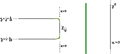
Figure 1. The curves $\gamma_{i,j}$ and $\gamma^{\uparrow}$.

Let $\gamma\subset\mathbb{R}^{2}$ and $f_{\gamma}$ be as above. Following [7, 6] there is a (weakly) filtered $A_{\infty}$-functor, called an inclusion functor, $\mathcal{I}_{\gamma}:\mathcal{F}uk(M)\longrightarrow\mathcal{F}uk(\mathbb{R}^{2}\times M)$ which sends the object $L\in\text{Obj}(\mathcal{F}uk(M))$ to $\gamma\times L\in\text{Obj}(\mathcal{F}uk(\mathbb{R}^{2}\times M))$.

Let $V\subset\mathbb{R}^{2}\times M$ be a Lagrangian cobordism. Denote by $\mathcal{V}$ the (weakly) filtered Yoneda module of $V$ and consider the pull-back module $\mathcal{I}_{\gamma}^{*}\mathcal{V}$. Note that for every exact Lagrangian $N\subset M$ we have

$$\mathcal{I}_{\gamma}^{*}\mathcal{V}(N)=CF(\gamma\times N,V)$$

as filtered chain complexes. (The filtrations are induced by $f_{V}$, $f_{\gamma,N}$ and by the Floer data in case it is not trivial.)

Assume that the ends of $V$ are $L_{1},\ldots,L_{k}$ and moreover that $V$ is cylindrical over $(-\infty,-\delta]\times\mathbb{R}$ for some $\delta>0$. (This can always be achieved by a suitable translation along the $x$-axis.) Fix $1\leq i\leq k-1$ and consider the curve $\gamma_{i,i+1}$ and the pull-back (weakly) filtered module $\mathcal{I}_{\gamma_{i,i+1}}^{*}\mathcal{V}$. By the results of [7, 8] there exists a module homomorphism

$$\Gamma_{V,\gamma_{i,i+1}}:L_{i+1}\longrightarrow L_{i}$$

which preserves action filtrations and such that

$$\mathcal{I}_{\gamma_{i,i+1}}^{*}\mathcal{V}=T^{d_{i}}\text{cone}(L_{i+1}\xrightarrow{\Gamma_{V,\gamma_{i,i+1}}}L_{i})$$

as (weakly) filtered modules. Here $T$ stand for the grading-translation functor and the amount $d_{i}\in\mathbb{Z}$ by which we translate depends only on $i$. We will be more precise about the values of $d_{i}$ later on. The map $\Gamma_{V,\gamma_{i,i+1}}$ is canonically defined by $V$ and $\gamma_{i,i+1}$, up to a boundary in $\hom^{\leq 0}_{\text{mod}_{\mathcal{F}uk(M)}}(L_{i+1},L_{i})$. Therefore it gives rise to a well defined morphism in the homological persistence category $\mathcal{C}_{0}=H\bigl{(}\hom^{\leq 0}_{\text{mod}_{\mathcal{F}uk(M)}}(L_{i+1},L_{i})\bigr{)}$ which by abuse of notation we still denote by $\Gamma_{V,\gamma_{i,i+1}}\in\hom_{\mathcal{C}_{0}}(L_{i+1},L_{i})$.

The above can be generalized to several consecutive ends in a row as follows. Fix $1\leq i\leq j\leq k$.

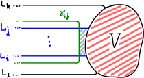
Figure 2. The module $\mathcal{I}_{\gamma_{i,j}}^{*}\mathcal{V}$.

The pull-back module $\mathcal{I}_{\gamma_{i,j}}^{*}\mathcal{V}$ can be identified with an iterated cone of the type:

$$\mathcal{I}_{\gamma_{i,j}}^{*}\mathcal{V}=\text{cone}\Bigl{(}L_{j}\longrightarrow\text{cone}\bigl{(}L_{j-1}\longrightarrow\ldots\longrightarrow\text{cone}(L_{i+1}\longrightarrow L_{i})\ldots\bigr{)}\Bigr{)},$$ (91)

where similarly to the case $\Gamma_{V,\gamma_{i,i+1}}$, all the maps in the iterated cone are module homomorphism that preserve filtrations. See figure 2.

Note that there are some grading-translations in (91) which we have ignored. We will be more precise about this point later on when we consider iterated cones involving three objects.

Remark.

If $V$ has $k$ ends then for every $i\leq 1$ and $k\leq l$ we have $\mathcal{I}_{\gamma_{i,l}}^{*}\mathcal{V}=\mathcal{I}_{\gamma^{\uparrow}}^{*}\mathcal{V}$.

Finally, fix $1\leq i\leq l<j\leq k$, and consider the two modules $\mathcal{I}_{\gamma_{i,l}}^{*}\mathcal{V}$ and $\mathcal{I}_{\gamma_{l+1,j}}^{*}\mathcal{V}$. There is a module homomorphism $\Gamma_{V,\gamma_{i,l},\gamma_{l+1,j}}:\mathcal{I}_{\gamma_{l+1,j}}^{*}\mathcal{V}\longrightarrow\mathcal{I}_{\gamma_{i,l}}^{*}\mathcal{V}$ which preserves filtrations. Note that we have

$$\mathcal{I}^{*}_{\gamma_{i,j}}\mathcal{V}=T^{d_{i,l,j}}\text{cone}(\mathcal{I}^{*}_{\gamma_{l+1,j}}\mathcal{V}\xrightarrow{\Gamma_{V,\gamma_{i,l},\gamma_{l+1,j}}}\mathcal{I}^{*}_{\gamma_{i,l}}\mathcal{V}),$$

for some $d_{i,l,j}\in\mathbb{Z}$. See Figure 3.

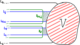
Figure 3. The modules $\mathcal{I}_{\gamma_{l+1,j}}^{*}\mathcal{V}$ and $\mathcal{I}_{\gamma_{i,l}}^{*}\mathcal{V}$.

6.6.4. Shadow of cobordisms

Recall from [8, 15] that for each Lagrangian cobordism $V\subset\mathbb{R}^{2}\times M$ we can associate its shadow $\mathcal{S}(V)$ defined by

$$\mathcal{S}(V):=Area\bigl{(}\mathbb{R}^{2}\setminus\mathcal{U}\bigr{)},$$ (92)

where $\mathcal{U}\subset\mathbb{R}^{2}\setminus\pi(V)$ is the union of all the unbounded connected components of $\mathbb{R}^{2}\setminus\pi(V)$.

6.6.5. $r$-acyclic objects

Let $V\subset\mathbb{R}^{2}\times M$ be a cobordism with ends $L_{1},\ldots,L_{k}$ such that $V$ is cylindrical over $(-\infty,-\delta]\times\mathbb{R}$ for some $\delta>0$. Let $\mathcal{S}(V)$ be the shadow of $V$ and denote by $e$ the area of the region to the right of $\gamma^{\uparrow}$ enclosed between $\gamma^{\uparrow}$ and the projection to $\mathbb{R}^{2}$ of the non-cylindrical part of $V$. See Figure 4.

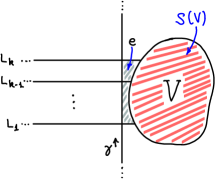
Figure 4. The projection of a cobordism to $\mathbb{R}^{2}$, its shadow $\mathcal{S}(V)$ and the area $e$.

The module $\mathcal{I}_{\gamma^{\uparrow}}^{*}\mathcal{V}=\mathcal{I}_{\gamma_{1,k}}^{*}\mathcal{V}$ (which also has the description (91) with $i=1$, $j=k$) is $r$-acyclic, where $r:=\mathcal{S}(V)+e$. This can be easily seen from the fact that $V$ can be Hamiltonian isotoped to a cobordism $W$ which is disjoint from $\gamma^{\uparrow}\times M$ via a compactly supported Hamiltonian isotopy whose Hofer length is $\leq r$. Standard Floer theory then implies that $\mathcal{I}_{\gamma^{\uparrow}}^{*}\mathcal{V}$ is acyclic of boundary depth $\leq r$. In the terminology used in this paper this means that the object $\mathcal{I}_{\gamma^{\uparrow}}^{*}\mathcal{V}$ is $r$-acyclic.

Remark 6.6.1.

The area summand $e$ that adds to the shadow of $V$ in the quantity $r$ can be made arbitrarily small at the expense of applying appropriate shifts to each of the ends $L_{i}$ of $V$. One way to do this is to replace the curve $\gamma^{\uparrow}$ by a curve $\gamma_{V}^{\uparrow}$ that coincides with $\gamma^{\uparrow}$ outside a compact subset and such that $\gamma_{V}^{\uparrow}$ approximates the shape of the projection of the non-cylindrical part of $V$ in such a way that the area $e^{\prime}$ enclosed between $\gamma^{\uparrow}_{V}$ and $\pi(V)$ is small. See Figure 5. One can apply a similar modification to the curves $\gamma_{i,j}$. Note that, in contrast to $f_{\gamma^{\uparrow}}$, the primitive $f_{\gamma_{V}^{\uparrow}}$ can no longer be assumed to be $0$ (a similar remarks applies to the primitives of the modifications of $\gamma_{i,j}$). As a result the cone decompositions (91) associated to the pullback modules $\mathcal{I}^{*}_{\gamma_{i,j}}$ will have the same shape but each of the Lagrangians $L_{i},\ldots,L_{j}$ will gain a different shift in action. Note that this will also result in “tighter” weighted exact triangles than the ones we obtain below, in the sense of weights and various shifts on the objects forming these triangles.

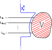
Figure 5. Replacing $\gamma^{\uparrow}$ by a curve $\gamma_{V}^{\uparrow}$ better approximating the shape of $V$.

To simplify the exposition, below we will not make these modifications and stick to the curves $\gamma^{\uparrow}$ and $\gamma_{i,j}$ as defined above, at the expense of $e$ not being necessarily small and the weights of the triangles not being necessarily optimal.

6.6.6. $r$-isomorphisms

We begin by visualizing the canonical map $\eta^{L}_{r}:\Sigma^{r}L\to L$, where $L\subset M$ is an exact Lagrangian. Consider the curve $\gamma\subset\mathbb{R}^{2}$ depicted in Figure 6, and let $r$ be the area enclosed between $\gamma$ and $\gamma^{\uparrow}$. Let $f_{\gamma}$ be the unique primitive of $\lambda_{\mathbb{R}^{2}}|_{\gamma}$ that vanishes along the lower end of $\gamma$. Note that $f_{\gamma}\equiv r$ along the upper end of $\gamma$. Let $V=L\times\gamma$ an set $f_{V}:=f_{\gamma,L}$. Therefore, the primitives induced by $V$ on its ends are as follows: the primitive on the lower end coincides with $f_{L}$, while the primitive on the upper end coincides with $f_{L}+r$. In other words, the cobordism $V$ has ends $L$ and $\Sigma^{r}L$. Moreover, the map $\Gamma_{V,\gamma_{1,2}}:\Sigma^{r}L\to L$ induced by $V$ and $\gamma_{1,2}$ is precisely $\eta^{L}_{r}$.

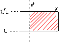
Figure 6. The cobordism inducing $\eta^{L}_{r}:\Sigma^{r}L\to L$.

Another source of geometric $r$-isomorphisms comes from Hamiltonian isotopies. Let $\phi_{t}^{H}$, $t\in[0,1]$ be a Hamiltonian isotopy and let $L\subset M$ be an exact Lagrangian. The Lagrangian suspension construction gives rise to an exact Lagrangian cobordism between $L$ and $\phi_{1}^{H}(L)$. After bending the ends of that cobordism to become negative one obtains a Lagrangian cobordism with negative ends being $L$ and $\phi_{1}^{H}(L)$. See Figure 7. The primitive $f_{V}$ on $V$ is uniquely defined by the requirement that $f_{V}$ coincides with $f_{L}$ on the lower end of $V$. The shadow $\mathcal{S}(V)$ of this cobordism equals the Hofer length of the isotopy $\{\phi_{t}^{H}\}_{t\in[0,1]}$, and we obtain an $r$-isomorphism $\phi_{1}^{H}(L)\to L$.

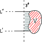
Figure 7. The Lagrangian suspension of a Hamiltonian isotopy, after bending the ends.

More generally, let $V$ be a Lagrangian cobordism with ends $L_{1},\ldots,L_{k}$. Let $r=\mathcal{S}(V)+e$ as above. Fix $1\leq l<k$. As explained above we have, up to an overall translation in grading,

$$\mathcal{I}^{*}_{\gamma^{\uparrow}}\mathcal{V}=\mathcal{I}^{*}_{\gamma_{1,k}}\mathcal{V}=\text{cone}(\mathcal{I}^{*}_{\gamma_{l+1,k}}\mathcal{V}\xrightarrow{\Gamma_{V,\gamma_{1,l},\gamma_{l+1,k}}}\mathcal{I}^{*}_{\gamma_{1,l}}\mathcal{V}),$$

and since $\mathcal{I}^{*}_{\gamma^{\uparrow}}\mathcal{V}$ is $r$-acyclic the map $\Gamma_{V,\gamma_{1,l},\gamma_{l+1,k}}:\mathcal{I}^{*}_{\gamma_{l+1,k}}\mathcal{V}\longrightarrow\mathcal{I}^{*}_{\gamma_{1,l}}\mathcal{V}$ is an $r$-isomorphism.

6.6.7. Weighted exact triangles

Let $V\subset\mathbb{R}^{2}\times M$ be a Lagrangian cobordism with ends $L_{1},\ldots,L_{k}$. Let $V^{\prime}\subset\mathbb{R}^{2}\times M$ be the cobordism obtained from $V$ by bending the upper end $L_{k}$ clockwise around $V$ so that it goes beyond the end $L_{1}$ as in Figure 8. To obtain a cobordism according to our conventions, we need to further shift $V^{\prime}$ upwards by one so that its lower end has $y$-coordinate $1$ (instead of $0$). Clearly $V^{\prime}$ is also exact and $\mathcal{S}(V^{\prime})=\mathcal{S}(V)$. We fix the primitive $f_{V^{\prime}}$ for $V^{\prime}$ to be the unique one that coincides with $f_{V}$ on the ends $L_{1},\ldots,L_{k-1}$. A simple calculation shows that $f_{V^{\prime}}$ induces on the lowest end of $V^{\prime}$ the primitive $f_{L_{k}}-r$, where $r=\mathcal{S}(V)+e+\epsilon$. (Here $\epsilon$ can be assumed to be arbitrarily small. It can be estimated from above by the area enclosed between the bent end corresponding to $\ell_{k}$, the projection to $\mathbb{R}^{2}$ of the non-cylindrical part of $V$, $\ell_{1}$ and $\gamma^{\uparrow}$. See Figure 8.)

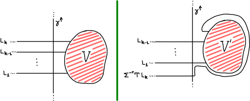
Figure 8. Bending the upper end $L_{k}$ of a cobordism $V$.

Taking into account grading (in case $V$ is graded in the sense of Floer theory), one can easily see that the grading on the lowest end of $V^{\prime}$ is translated by $1$ in comparison to $L_{k}$. Summing up, the above procedure transforms a cobordism $V$ with ends $L_{1},\ldots,L_{k}$ into a cobordism $V^{\prime}$ with ends $\Sigma^{-r}TL_{k},L_{1},\ldots,L_{k-1}$.

Similarly, one can take $V$ and bend its lowest end $L_{1}$ counterclockwise around $V$ and obtain a new cobordism $V^{\prime\prime}$ with ends $L_{2},\ldots,L_{k},\Sigma^{r}T^{-1}L_{1}$ and with $\mathcal{S}(V^{\prime\prime})=\mathcal{S}(V)$.

We are now in position to describe geometrically weighted exact triangles. Let $V$ be a cobordism with three ends, which for compatibility with Definition 4.2.1 we denote by $C,B,A$ (going from the lowest end upward). See Figure 9.

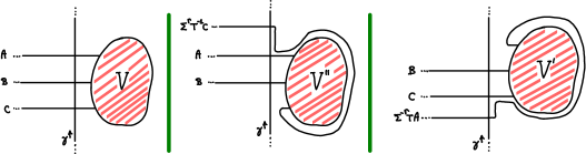
Figure 9. A cobordism leading to an exact triangle of weight $r$.

Let $r=\mathcal{S}(V)+e+\epsilon$. Put

$$\bar{u}:=\Gamma_{V,\gamma_{2,3}}:A\to B,\quad\bar{v}:=\Gamma_{V,\gamma_{2,1}}:B\to C.$$

Consider also the counterclockwise rotation $V^{\prime\prime}$ of $V$ whose ends are $B,A,\Sigma^{r}T^{-1}C$. Let

$$\bar{w}:=\Sigma^{-r}T\Gamma_{V^{\prime\prime},\gamma_{2,3}}=\Gamma_{V^{\prime},\gamma_{1,2}}:C\to\Sigma^{-r}TA.$$

We claim that

$$A\xrightarrow{\bar{u}}B\xrightarrow{\bar{v}}C\xrightarrow{\bar{w}}\Sigma^{-r}TA$$ (93)

is a strict exact triangle of weight $r$. This triangle is based on the genuinely exact triangle from $\mathcal{C}_{0}$:

$$A\xrightarrow{u}B\xrightarrow{v}C^{\prime}\xrightarrow{w}TA,$$ (94)

where $u=\bar{u}$, $C^{\prime}=\mathcal{I}^{*}_{\gamma_{2,3}}V=\text{cone}(A\xrightarrow{u}B)$, $v:B\to C^{\prime}$ is the standard inclusion and $w:C^{\prime}\to TA$ the standard projection. The $r$-isomorphism $\phi:C^{\prime}\to C$ and its right $r$-inverse $\psi:\Sigma^{r}C\to C^{\prime}$ are as follows:

$$\phi=\Gamma_{V,\gamma_{1,1},\gamma_{2,3}},\quad\psi=T\Gamma_{V^{\prime\prime},\gamma_{1,2},\gamma_{3,3}}:\Sigma^{r}C\to T\mathcal{I}_{\gamma_{1,2}}^{*}V^{\prime\prime}=C^{\prime}.$$

Note that $\mathcal{I}_{\gamma_{1,2}}^{*}V^{\prime\prime}=T^{-1}\mathcal{I}_{\gamma_{2,3}}^{*}V=T^{-1}C^{\prime}=T^{-1}\text{cone}(A\xrightarrow{u}B)$.

The fact that $\psi$ is a right $r$-inverse to $\phi$ and that these maps fit into the diagram (25) follows from standard arguments in Floer theory. Note that these statements do not hold on the chain level, but only in $\mathcal{C}_{0}$.

6.6.8. Rotation of triangles

Let $V$ be a cobordism with three ends $C,B,A$ as in §6.6.7 and consider the exact triangle (93) of weight $r$. Let $V^{\prime}$ be the clockwise rotation of $V$, with ends $B,C,\Sigma^{-r}TA$. The exact triangle associated to $V^{\prime}$ is

$$B\xrightarrow{\bar{v}}C\xrightarrow{\bar{w}}\Sigma^{-r}TA\xrightarrow{\bar{u}^{\prime}}\Sigma^{-r-\epsilon^{\prime}}TB,$$ (95)

where $\epsilon^{\prime}$ can be assumed to be arbitrarily small. It is not hard to see that in $\mathcal{C}_{\infty}$ (up to identifying objects with their shifts and ignoring signs in the maps) the exact triangle (95) is precisely the rotation of the exact triangle corresponding to (93) in $\mathcal{C}_{\infty}$.

The above shows that rotation of weighted exact triangles coming from cobordisms with three ends preserves weights (up to an arbitrarily small error). Interestingly this is sharper than the case in a general TPC, described in Proposition 4.2.5, where the weight of a rotated triangle doubles. See also Remark 4.2.7.

6.6.9. Weighted octahedral property

The weighted octahedral formula from Proposition 4.2.8 admits too a geometric interpretation in the realm of cobordisms. We will not give the details of this construction here. Instead we will briefly explain the cobordism counterpart of cone refinement and why it behaves additively with respect to weights, as described algebraically in Proposition 4.3.2. Note that weighted cone-refinement is one of the main corollaries of the weighted octahedral property.

For simplicity we focus here on the case described in Example 4.3.3 and ignore the grading-translation $T$. Assume that we have two cobordisms $V$ with ends $X,B,A$ and $U$ with ends $A,F,E$.

These cobordisms induce two weighted exact triangles of weights $r=\mathcal{S}(V)+e_{V}+\epsilon$ and $s=\mathcal{S}(U)+e_{U}+\epsilon$. By gluing the two cobordisms along the ends corresponding to $A$ we obtain a new cobordism $W$ with four ends $X,B,F,E$. See Figure 10. By the previous discussion this exhibits $X$ as an iterated cone with linearization $(B,F,E)$ which corresponds precisely to the algebraic cone refinement of $X$ with linearization $(B,A)$ by $A$ with linearization $(F,E)$.

Clearly the shadow $\mathcal{S}(W)$ of $W$ equals to $\mathcal{S}(U)+\mathcal{S}(V)$, and the total weight of the cone decomposition of $X$ associated to $W$ is $r+s$. Note again, that by the procedure explained in Remark 6.6.1 one can make the errors $e_{V}$, $e_{U}$ small at the expense of applying some shifts to the elements of the linearization.

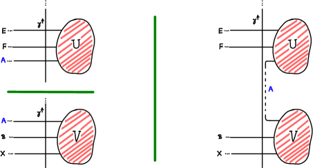
Figure 10. Cone refinement via gluing cobordisms along two ends.

6.7. Work in progress (towards algebra 102)

There are a few immediate questions and properties that we are currently working on but have decided not to include in this paper.

• We have not discussed idempotents and split completion in the triangulated persistence category setting. It turns out that the notion natural in this setting is a sort of refinement of the usual Karoubi completion. Given a TPC $\mathcal{C}$, it is obvious that the starting point in the construction is to consider the split completion of the $0$-level, $\mathcal{C}_{0}$ in the usual triangulated category sense. However, it is immediate to see that this will not lead to an $\infty$-level that is split complete. One needs to also complete with respect to pseudo-idempotents $e:\Sigma^{r}X\to X$ that are such that $e\circ\Sigma^{r}e=e\circ\eta_{r}$. This turns out to be possible but a bit more complicated compared to Karoubi completion.

• Given a TPC, $\mathcal{C}$, there are two natural associated Grothendieck groups: $K_{0}^{0}=K_{0}(\mathcal{C}_{0})$ and $K_{0}^{\infty}=K_{0}(\mathcal{C}_{\infty})$. Assume that $d^{\mathcal{F}}$ is one of the fragmentation pseudo-metrics on $\mathcal{C}$ as in Definition 4.3.5 (one could also use instead the pseudo-metrics such as $\overline{d}^{\mathcal{F}}$ on $\mathcal{C}_{\infty}$ as reviewed in §5.4) associated to a family $\mathcal{F}$ that is invariant with respect to shift (in the sense that if $F\in\mathcal{F}$, then $\Sigma^{r}F\in\mathcal{F}$ for all $r\in\mathbb{R}$). It is not difficult to see that such a pseudo-metric induces a pseudo-metric $d^{\mathcal{F}}$ on $K_{0}^{0}$. This pseudo-metrics is translation invariant and thus characterized by a group-pseudo-norm defined by $\nu^{\mathcal{F}}(a)=d^{\mathcal{F}}(a,0)$. Moreover, the shift functor $\Sigma^{r}$ induces a flow on $K_{0}^{0}$ and $\nu^{\mathcal{F}}$ is constant along the orbits of this flow. In short, $K_{0}^{0}$ is a topological abelian group with an interesting structure that can be used to study the action of various groups of automorphisms of the initial category. For instance, in the symplectic examples, the Hamiltonian diffeomorphism group, $\mathrm{Ham}(M)$, of the underlying symplectic manifold $(M,\omega)$ admits a natural, continuous representation in $\mathrm{Aut}(K_{0}^{0})$ (where the relevant TPC is one of the filtered Fukaya categories discussed above). Here $\mathrm{Aut}(K_{0}^{0})$ are the group automorphisms endowed with a topology induced by the group pseudo-norm defined by $\overline{\nu}^{\mathcal{F}}(\phi)=\sup_{a}\nu^{\mathcal{F}}(\phi(a)-a)$. The topology on $\mathrm{Ham}(M)$ is the one induced by the Hofer norm. Given the properties of the Hamiltonian diffeomorphism group (for instance, the fact that it is simple for closed manifolds), it seems to be an interesting question to study when this representation is non-trivial. There are similar properties for the group $K_{0}^{\infty}$, except that this group is much smaller.

• Another natural direction of investigation is localization and derived functors in the setting of TPCs. There are two natural classes with respect to which one can localize: the $0$-isomomorphism and the $r$-isomorphisms with $r\in(0,\infty)$ variable. In both cases, one can construct filtered versions of the localization of $\mathcal{C}$ with respect to the respective class of morphisms and one can verify that both localizations are again TPCs. It is also possible to consider persitence derived categories associated to persistence categories as well as persistence derived functors associated to persistence functors.

• In [5] are introduced certain cobordism categories called with surgery models and it is shown that they give rise to triangulated categories with objects immersed Lagrangian submanifolds and with morphisms certain classes of immersed cobordisms relating them. It is expected that by taking into account the shadows of these cobordisms - in the sense in §6.6.4 - one can extract a TPC refinement of that category.

Of course, there are also a variety of other algebraic and geometric questions, such as reformulating parts of this machinery in a Waldhausen type category setting (as mentioned in §6.3) as well as symplectic applications deduced by pursuing the properties of the TPCs relevant in that context.

References

- [1] Tomohiro Asano and Yuichi Ike. Persistence-like distance on Tamarkin’s category and symplectic displacement energy. J. Symp. Geom, 18(3):613–649, 2020.
- [2] Serguei Barannikov. The framed Morse complex and its invariants. In Singularities and bifurcations, volume 21 of Adv. Soviet Math., pages 93–115. Amer. Math. Soc., Providence, RI, 1994.
- [3] Ulrich Bauer and Michael Lesnick. Induced matchings and the algebraic stability of persistence barcodes. J. Comput. Geom., 6(2):162–191, 2015.
- [4] Paul Biran and Octav Cornea. Bounds on the Lagrangian spectral metric in cotangent bundles. arXiv: 2008.04756.
- [5] Paul Biran and Octav Cornea. A Lagrangian pictionary. To appear in the Kyoto Math. Journal.
- [6] Paul Biran and Octav Cornea. Lagrangian cobordism. I. J. Amer. Math. Soc., 26(2):295–340, 2013.
- [7] Paul Biran and Octav Cornea. Lagrangian cobordism and Fukaya categories. Geom. Funct. Anal., 24(6):1731–1830, 2014.
- [8] Paul Biran, Octav Cornea, and Egor Shelukhin. Lagrangian shadows and triangulated categories. To appear in Astérisque. Can be found at http://arxiv.org/pdf/1806.06630v1.
- [9] Alexey I Bondal and Mikhail M Kapranov. Enhanced triangulated categories. Mathematics of the USSR-Sbornik, 70(1):93, 1991.
- [10] Peter Bubenik and Nikola Milićević. Homological algebra for persistence modules. Foundations of Computational Mathematics, pages 1–46, 2019.
- [11] François Charest and Chris Woodward. Floer trajectories and stabilizing divisors. J. Fixed Point Theory Appl., 19(2):1165–1236, 2017.
- [12] Frédéric Chazal, Vin de Silva, Marc Glisse, and Steve Oudot. The structure and stability of persistence modules. SpringerBriefs in Mathematics. Springer, [Cham], 2016.
- [13] Octav Cornea and François Lalonde. Cluster homology: an overview of the construction and results. Electron. Res. Announc. Amer. Math. Soc., 12:1–12, 2006.
- [14] Octav Cornea, Gregory Lupton, John Oprea, and Daniel Tanré. Lusternik-Schnirelmann category, volume 103 of Mathematical Surveys and Monographs. American Mathematical Society, Providence, RI, 2003.
- [15] Octav Cornea and Egor Shelukhin. Lagrangian cobordism and metric invariants. Journal of Differential Geometry, 112:1–45, 2019.
- [16] Octavian Cornea. Cone-length and lusternik-schnirelmann category. Topology, 33:95–111, 1994.
- [17] Octavian Cornea. There is just one rational cone-length. Trans. Amer. Math. Soc., 344(2):835–848, 1994.
- [18] William Crawley-Boevey. Decomposition of pointwise finite-dimensional persistence modules. J. Algebra Appl., 14(5):1550066, 8, 2015.
- [19] George Dimitrov, Fabian Haiden, Ludmil Katzarkov, and Maxim Kontsevich. Dynamical systems and categories, volume 621 of Contemp. Math., pages 133–170. Amer. Math. Soc., Providence, RI, 2014.
- [20] Vladimir Drinfeld. DG quotients of DG categories. J. Algebra, 272(2):643–691, 2004.
- [21] Herbert Edelsbrunner. A short course in computational geometry and topology. SpringerBriefs in Applied Sciences and Technology. Springer, Cham, 2014.
- [22] Yu-Wei Fan and Simion Filip. Asymptotic shifting numbers in triangulated categories. arXiv: 2008.06159.
- [23] Yves Félix, Stephen Halperin, and Jean-Claude Thomas. Rational homotopy theory, volume 205 of Graduate Texts in Mathematics. Springer-Verlag, New York, 2001.
- [24] Kenji Fukaya, Paul Seidel, and Ivan Smith. Exact Lagrangian submanifolds in simply-connected cotangent bundles. Invent. Math., 172(1):1–27, 2008.
- [25] Kenji Fukaya, Paul Seidel, and Ivan Smith. The symplectic geometry of cotangent bundles from a categorical viewpoint, volume 757 of Lecture Notes in Phys., pages 1–26. Springer, Berlin, 2009.
- [26] Phillip Griffiths and Joseph Harris. Principles of algebraic geometry. Wiley-Interscience [John Wiley & Sons], New York, 1978. Pure and Applied Mathematics.
- [27] Misha Gromov. Metric structures for Riemannian and non-Riemannian spaces. Modern Birkhäuser Classics. Birkhäuser Boston, Inc., Boston, MA, english edition, 2007. Based on the 1981 French original, With appendices by M. Katz, P. Pansu and S. Semmes, Translated from the French by Sean Michael Bates.
- [28] Stéphane Guillermou, Masaki Kashiwara, and Pierre Schapira. Sheaf quantization of Hamiltonian isotopies and applications to nondisplaceability problems. Duke Math. J., 161(2):201–245, 2012.
- [29] Stéphane Guillermou and Pierre Schapira. Microlocal theory of sheaves and Tamarkin’s non displaceability theorem. In Homological mirror symmetry and tropical geometry, volume 15 of Lect. Notes Unione Mat. Ital., pages 43–85. Springer, Cham, 2014.
- [30] Felix Hensel. Stability conditions and Lagrangian cobordisms. J. Symplectic Geom., 18(2):463–536, 2020.
- [31] Masaki Kashiwara and Pierre Schapira. Sheaves on manifolds, volume 292 of Grundlehren der Mathematischen Wissenschaften [Fundamental Principles of Mathematical Sciences]. Springer-Verlag, Berlin, 1990. With a chapter in French by Christian Houzel.
- [32] Pierre Lelong. Intégration sur un ensemble analytique complexe. Bull. Soc. Math. France, 85:239–262, 1957.
- [33] Dimitri Orlov. Triangulated categories of singularities, and equivalences between Landau-Ginzburg models. Mat. Sb., 197(12):117–132, 2006.
- [34] Dmitri Orlov. Remarks on generators and dimensions of triangulated categories. Mosc. Math. J., 9(1):153–159, back matter, 2009.
- [35] Leonid Polterovich, Daniel Rosen, Karina Samvelyan, and Jun Zhang. Topological persistence in geometry and analysis, volume 74 of University Lecture Series. AMS, Providence, RI, 2020.
- [36] Dieter Puppe. On the formal structure of stable homotopy theory. Colloquium on algebraic topology, Aarhus Universitet Matematisk Institute, pages 65–71, 1962.
- [37] Paul Seidel. Fukaya categories and Picard-Lefschetz theory. Zurich Lectures in Advanced Mathematics. European Mathematical Society (EMS), Zürich, 2008.
- [38] Nick Sheridan. On the homological mirror symmetry conjecture for pairs of pants. J. Differential Geom., 89(2):271–367, 2011.
- [39] Steve Smale. On the topology of algorithms. I. J. Complexity, 3(2):81–89, 1987.
- [40] Dennis Sullivan. Infinitesimal computations in topology. Inst. Hautes Études Sci. Publ. Math., (47):269–331 (1978), 1977.
- [41] Dmitry Tamarkin. Microlocal condition for non-displaceability. In Algebraic and analytic microlocal analysis, volume 269 of Springer Proc. Math. Stat., pages 99–223. Springer, Cham, 2018.
- [42] Michael Usher. Boundary depth in Floer theory and its applications to Hamiltonian dynamics and coisotropic submanifolds. Israel J. Math., 184:1–57, 2011.
- [43] Michael Usher. Hofer’s metrics and boundary depth. Ann. Sci. Éc. Norm. Supér. (4), 46(1):57–128 (2013), 2013.
- [44] Michael Usher and Jun Zhang. Persistent homology and Floer-Novikov theory. Geom. Topol., 20(6):3333–3430, 2016.
- [45] Jean-Louis Verdier. Catégories dérivées: quelques résultats (état 0). In Cohomologie étale, volume 569 of Lecture Notes in Math., pages 262–311. Springer, Berlin, 1977.
- [46] Charles A. Weibel. An introduction to homological algebra, volume 38 of Cambridge Studies in Advanced Mathematics. Cambridge University Press, Cambridge, 1994.
- [47] Jun Zhang. Quantitative Tamarkin Theory. CRM Short Courses; Virtual Series on Symplectic Geometry. Springer International Publishing, 2020.
- [48] Afra Zomorodian and Gunnar Carlsson. Computing persistent homology. Discrete Comput. Geom., 33(2):249–274, 2005.