Linear inference problems with deterministic constraints–LABEL:lastpage

Linear inference problems with deterministic constraints

Methods are described for the solution of linear inference problems subject to deterministic constraints. The approach builds on work by [Backus (1970a), Backus (1970b), Backus (1970c)] and [Parker (1977)], but a range useful advances are suggested to address both conceptual and practical issues. The theory is motivated by, and illustrated with, the estimation of a finite number of a function’s spherical harmonic coefficients from a finite set of its point values. Numerical examples are included to demonstrate that the methods can be efficiently applied to realistic problems.

1 Introduction

This paper describes methods for solving linear inference problems. Any work of this topic owes a profound debt to [Backus & Gilbert (1968), Backus & Gilbert (1967), Backus & Gilbert (1970)], [Backus (1970a), Backus (1970b), Backus (1970c), Backus (1972), Backus (1988), Backus (1989), Backus (1996)], and [Parker (1972), Parker (1977)], along with other notable contributions including [Pijpers & Thompson (1992), Pijpers & Thompson (1994)], [Genovese & Stark (1996)], [Evans & Stark (2002)], and [Stark (2008)]. At the outset it is worth stating clearly what is meant by an inference problem as opposed to an inverse problem. Within each we are given data that is related in a specified manner to an unknown model. In broad terms, the inverse problem seeks to recover the unknown model as best as possible. By contrast, an inference problem aims merely to estimate finitely-many numerical properties of the model that are of interest.

From a solution of an inverse problem one can trivially obtain a corresponding solution for an associated inference problem. But not all solutions of inference problems need be obtained in this manner, with such an approach generally being sub-optimal both theoretically and computationally. The basic reason is that while inverse problems with finite data generically have an infinite-fold non-uniqueness, only a finite-dimensional component of this non-uniqueness is seen by the properties estimated within an inference problem. As a result, while uncertainty quantification within inverse problems remains very difficult (from a computationally perspective if nothing else), significantly more can be done within the context of an inference problem. This point is especially relevant to situations where the physics and data are such that no plausible reconstruction of the model can be obtained (Parker, 1972).

To give one example, consider lateral density variations in the lowermost mantle, and particularly with regard to the two large low shear velocity provinces (LLSVPs) whose nature and geodynamic significance remains unclear. The geophysical observations that are sensitive to any such density variations are principally: low-frequency free oscillations, body tides, and long-wavelength geoid anomalies (e.g. Ishii & Tromp, 1999; Lau et al., 2017). However, these observations see only very broad spatial averages of lower-mantle lateral density variations (along with other parameters). There is no physical basis for believing that structures do not exist in the lower mantle below the resolvable length-scales. And hence inversion of this data must always lead to models that are overly smooth and contain substantial uncertainties which are difficult to quantify. A quite different approach would be simply to ask what the average density anomalies within the two LLSVPs are. This is an inference problem in which only two numbers are to be estimated, but if it could be solved – meaning all plausible average densities are determined – then the result would be of unquestionable value in understanding the deep Earth.

It might here be added more generally that geophysical inference problems are necessarily associated with specific quantitative questions about the Earth. In contrast, geophysical inverse problems generally focus on model building, this usually being done in the hope that some new and interesting qualitative feature will be discovered. Both approaches have value, of course. And a model building exercise that reveals an interesting feature might be followed by a more targeted study that asks specific quantitative questions. Indeed, this is precisely what is suggested above with regard to lower mantle density. But it is important to remember that inverse and inference problems are distinct in their aims; this is reflected in the methods developed, and the manner in which their efficacy should be judged.

It is the author’s experience that the literature on inference problems is considerably less well known within geophysics than that on inverse problems. This seems a shame, particularly so because this approach came first, from within our community, and was motivated directly by the grossly under-determined problems that are familiar to us, but comparatively rare in other parts of physics. Perhaps most have at least heard of Backus-Gilbert theory, but often only as a historical curiosity that might be cited but need not be understood. There are exceptions, of course, including the recent work of Zaroli (2016, 2019) who applied a variant of Backus-Gilbert theory to linearised seismic tomography. But even these admirable studies have been done in seeming ignorance of later work by Backus and others. It is only here that the qualitative approach to uncertainties within Backus-Gilbert theory based on resolution length is replaced by a fully quantitative theory in which the need for suitable prior constraints is made clear.

Why then have inference problems received comparatively little attention in recent times? Here one can only speculate, but there seem to be two issues. The first is that the numerical cost of the methods was thought to be prohibitively high. For example, Parker (1977) described a method for solving linear inference problems with a prior norm bound in the error-free case. To do this it is necessary to invert a square matrix with dimension equal to the sum of the number of data and the number of quantities to be estimated. At the time these linear systems were simply too large within any real application. Moreover, while Parker discussed in outline how random data errors could be incorporated into the problem, the method’s numerical implementation would be both complicated and require a substantial increase in costs. Parker concluded that his approach, while theoretically superior, was simply not competitive with the discretised least squares methods that had become popular (e.g Wiggins, 1972). Times change, however, and what was once impossible numerically is now routine. In particular, iterative matrix-free methods mean that there need be no difficulty in solving linear equations in high-dimensional spaces. Indeed, an important contribution of Zaroli (2016, 2019) was to show that the oft-stated objection to applying Backus-Gilbert theory to large-scale problems can be overcome through the application of modern computational techniques. In a similar manner, this paper describes a new approach to solving linear inference problems that is computationally efficient and well-suited to problems with large data sets. In the error-free case the theory is equivalent to that in Backus (1970a) and Parker (1977), but significant computational savings are made possible through both the formulation of the theoretical results and the numerical methods applied. To incorporate data errors a new approach is developed that builds on the largely qualitative discussion in Parker (1977). While there is an increase in computational costs over the error-free case, the method remains practically feasible for realistic applications. This new approach also has the advantage of working not just in the case of Gaussian errors, but also for a wider class of unimodal distributions.

The second point that seems to limit work on linear inference problems is the perceived difficulty of the literature. In almost all geophysical inverse and inference problems the model comprises a function belonging to an infinite-dimensional vector space. In discussing these problems it is, therefore, necessary to use the methods and language of functional analysis, albeit only at a low level. Within papers on linear inference problems this has always been done, and it is true for this paper also. In contrast much work on geophysical inverse problems assumes from the outset a finite-dimensional model space (e.g. Tarantola, 2005; Wunsch, 2006; Menke, 2018). This is not, of course, to say that function space methods are not used within the literature on geophysical inverse theory (e.g. Parker, 1994), but only that such techniques can be avoided by those who do not know, and will not learn, the necessary ideas. There is generally no physical reason for working with a finite-dimensional model space, however, and this step is done only to make the mathematics easier. If all that is desired are models that fit the data, then there is no harm in doing this so long as the discretised space is sufficiently large. However, as soon as questions of uncertainty arise, then by limiting the size of the model space it is inevitable that errors will be underestimated. The extent to which this matters is necessarily application dependent, but usually cannot be quantified. The issue can perhaps be mitigated by allowing the dimension of the approximating space to vary (e.g. Sambridge et al., 2006), but in practice the range of dimensions explored is small.

The passage from finite- to infinite-dimensions is in some respects easy, and yet in others rather subtle. Properties that can be taken for granted in finite-dimensions can be lost, while entirely new phenomena can occur. For example, in finite-dimensional linear problems the model space has a unique topology, but in infinite-dimensions the model space topology must be specified as an essential part of the problem’s formulation. Moreover, there is usually a choice about what topology is selected, and hence one needs to carefully consider how this is done. In almost all the literature on geophysical inference problems, however, the model space has been assumed to be a Hilbert space. But this has largely been done for convenience, with most geophysical problems being more naturally posed on Banach spaces. Notable exceptions are Evans & Stark (2002) and Stark (2008) who generalised Backus-Gilbert estimators from the perspective of statistical inference theory. A specific aim of this paper is the formulation and characterisation of linear inference problems in a Banach space. While there are links to what is done in Evans & Stark (2002) and Stark (2008), the focus here is primarily on ideas found in Backus’ later work done independently of Gilbert. In particular, three key results given by Backus (1970a) for problems in Hilbert spaces are generalised and extended. It will be shown that while a complete theory can be developed in a Banach space setting, its implementation requires the solution of some very difficult, and perhaps intractable, optimisation problems (c.f. Stark, 2015). As a pragmatic step, the results are then reduced to the Hilbert space case for which the necessary calculations are easy. In contrast to earlier work, however, this simplifying step is made explicit, and a discussion is given as to how an appropriate Hilbert space can be both identified and justified.

As noted, work on linear inference problems necessitates a basic understanding of functional analysis, and this has likely been an impediment to people who might otherwise be interested. Moreover, in trying to present new ideas in this field it cannot be reasonably assumed that all readers will be conversant with what has been done previously. As a result, this paper has been written to be largely self-contained, while appendices are included to summarise mathematical concepts and notations that may be unfamiliar. In doing this there is a cost in terms of length, while some potentially routine material needs to be repeated. But it is hoped that this approach makes for an easier read, though perhaps still not an easy one. Chapter 1 of Parker (1994) also provides a nice introduction to functional analysis, and covers most of what it required in this work. Proofs are given either when a result is thought to be original, or if the argument is short and some useful insight can be gained. Readers who wish to skip any or all of the proofs should still be able to follow the the main arguments.

1.1 Spectral estimation from point data on a sphere

To explain further the aims of this paper, it will be useful to turn to a concrete inference problem motivated by the work of Hoggard et al. (2016) on dynamic topography. Let $\{x_{i}\}_{i=1}^{n}$ be a set of distinct points on the unit two-sphere, $\mathbb{S}^{2}$, and $u:\mathbb{S}^{2}\rightarrow\mathbb{R}$ an unknown continuous function. Suppose we are given the point values $\{u(x_{i})\}_{i=1}^{n}$, and from this data wish to estimate the function’s $(l,m)$th spherical harmonic coefficient. In practice, we might require simultaneous estimates of some finite number of spherical harmonic coefficients (e.g. all those at degree $l$ from which we could compute the associated power), while all real data are subject to errors. Such generalisations will be discussed later, but for the moment we keep the problem as simple as possible. Fig.1 shows an example of the data set along with the underlying function. In accordance with Hoggard et al. (2016), all points lie below sea level, and hence there are large regions of the domain where the function is completely unconstrained by the data.

An associated inverse problem can of course also be considered in this situation. Namely, the reconstruction of the unknown function from the given point data. Having done this by some means, the associated value of the $(l,m)$th spherical harmonic coefficient could then be extracted. This is precisely what Hoggard et al. (2016) did via a simple discretised least squares method. A range of other approaches are possible for reconstructing the function (e.g. Valentine & Davies, 2020), including function-space techniques designed specifically for interpolation of point data on a sphere (e.g. Freeden & Hermann, 1986). Error estimates on the solution of the inverse problem, if obtained, can be propagated through to the spherical harmonic coefficient, and hence uncertainties quantified. As noted previously, however, the optimal approach to solving an inference problems is not necessarily to first solve an inverse problem.

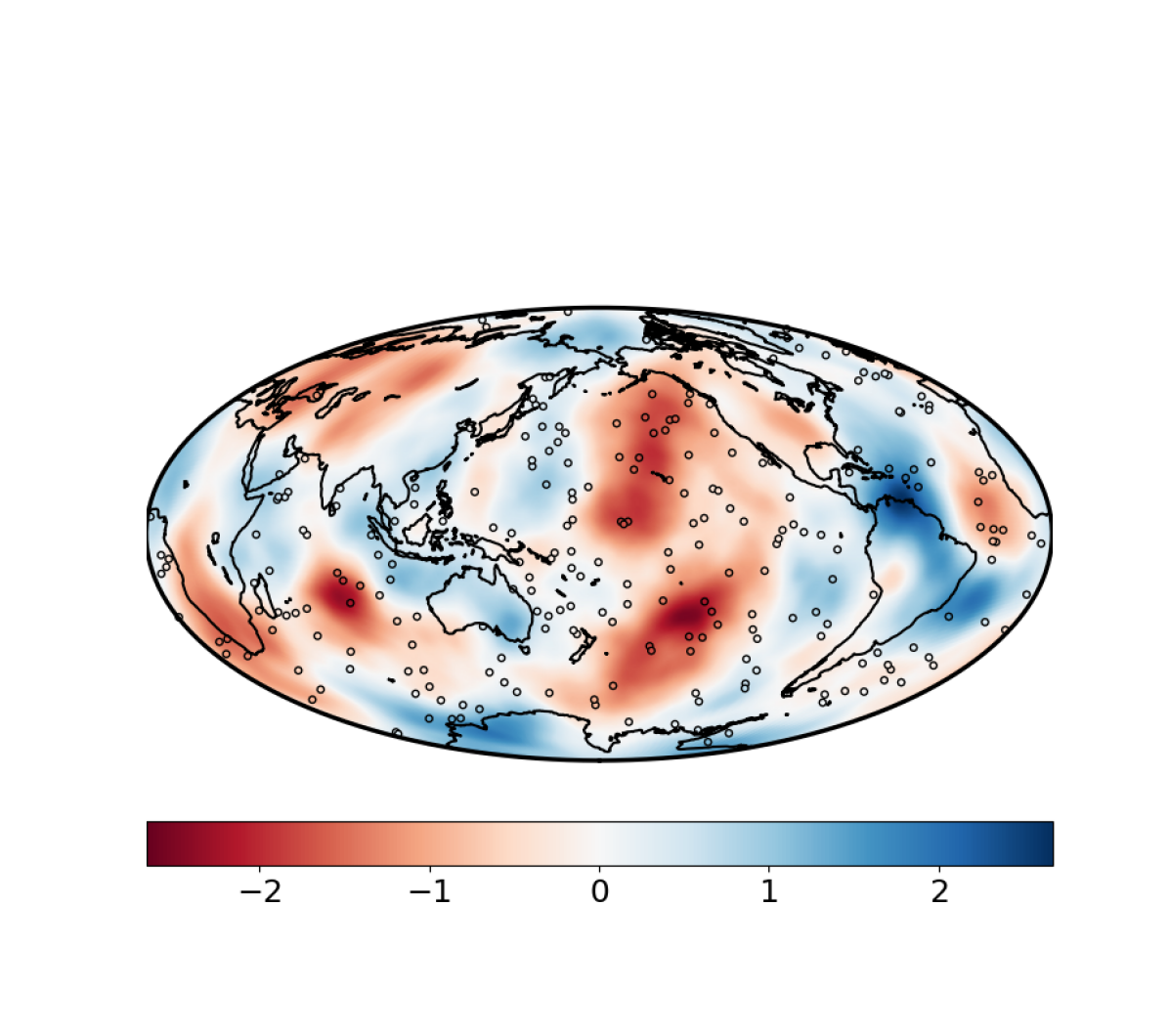
Figure 1: An example of a function on the unit sphere that has been sampled at 250 locations indicated by circular markers. The value of the function at each location is indicated by the colour of the circle using the same scale as the main plot. Coastlines are shown, and it can be seen that all sample locations have been chosen to lie below sea level. All map plots later in the paper have been made in an identical manner using the same colour scale.

We denote by $C^{0}(\mathbb{S}^{2})$ the set of all continuous real-valued functions on $\mathbb{S}^{2}$. Relative to the supremum norm

$$\|u\|_{C^{0}(\mathbb{S}^{2})}=\sup_{x\in\mathbb{S}^{2}}|u(x)|,$$ (1)

this is a Banach space. For each $x\in\mathbb{S}^{2}$, the mapping

$$u\mapsto u(x),$$ (2)

is a continuous linear functional on $C^{0}(\mathbb{S}^{2})$, and hence defines an element of the dual space $C^{0}(\mathbb{S}^{2})^{\prime}$ that we denote by $\delta_{x}$ and call the Dirac measure at $x$. The $i$th datum can then be written in the form

$$v_{i}=\left\langle{\delta_{x_{i}}},{u}\right\rangle,$$ (3)

where an angular bracket is used to denote a dual pairing. It is worth commenting that this relation might also be written

$$v_{i}=\int_{\mathbb{S}^{2}}\delta_{x_{i}}(x)\,u(x)\,\mathrm{d}S,$$ (4)

using the Dirac delta function on $\mathbb{S}^{2}$. Having done this, we could identify sensitivity kernel for the $i$th datum as a delta function based at the observation point. While this notation is familiar and suggestive, it does have a downside. While the right hand side of eq.(5) looks like an inner product in the space $L^{2}(\mathbb{S}^{2})$, this is not at all the case. There are inference problems on $L^{2}(\mathbb{S}^{2})$ for which the data takes the form

$$v_{i}=\int_{\mathbb{S}^{2}}k_{i}(x)\,u(x)\,\mathrm{d}S,$$ (5)

with the $i$th sensitivity kernel, $k_{i}$, is an element of $L^{2}(\mathbb{S}^{2})$. For such problems, the Hilbert space methods developed by Backus can be applied directly. But to confuse the present problem, posed in a more general Banach space, with the $L^{2}$-case can only lead to confusion (e.g. Gubbins, 2004, Chapter 9). Returning to the problem at hand, each spherical harmonic $Y_{lm}$ can be uniquely associated with a dual vector (denoted for simplicity with the same symbol) that is defined through

$$\left\langle{Y_{lm}},{u}\right\rangle=\int_{\mathbb{S}^{2}}u\,Y_{lm}\,\mathrm{d}S$$ (6)

where $\mathrm{d}S$ is the standard surface element on $\mathbb{S}^{2}$. For definiteness, fully normalised real spherical harmonics as defined in Appendix B of Dahlen & Tromp (1998) are used throughout this paper. Given this preamble, our first result shows that the data alone provide no information about the spherical harmonic coefficient of interest:

Proposition 1.1

For any $v_{1},\dots,v_{n},w\in\mathbb{R}$ there exists a (non-unique) function $u\in C^{0}(\mathbb{S}^{2})$ such that

$$v_{i}=\left\langle{\delta_{x_{i}}},{u}\right\rangle,\quad i\in\{1,\dots,n\},$$ (7)

while simultaneously $w=\left\langle{Y_{lm}},{u}\right\rangle$.

Proof: A simple constructive proof can be given using Urysohn’s Lemma (e.g. Kelley, 1955). First, we select disjoint open subsets $\{U_{i}\}_{i=1}^{n}$ of $\mathbb{S}^{2}$ such that $x_{1}\in U_{1},\dots,x_{n}\in U_{n}$. For each $i\in\{1,\dots,n\}$, we then choose $V_{i}$ to be open, properly contained in $U_{i}$, and have $x_{i}\in V_{i}$. Urysohn’s Lemma yields for each $i\in\{1,\dots,n\}$ a continuous function $\varphi_{i}:\mathbb{S}^{2}\rightarrow[0,1]$ such that $\varphi_{i}=1$ within $V_{i}$ and $\varphi_{i}=0$ on the complement of $U_{i}$. We now define the function

$$u=\sum_{i=1}^{n}v_{i}\varphi_{i}+\alpha\left(1-\sum_{i=1}^{n}\varphi_{i}\right)Y_{lm},$$ (8)

where $\alpha\in\mathbb{R}$ is to be determined. By construction $u(x_{i})=v_{i}$ for each $i\in\{1,\dots,n\}$, while on the complement of $\bigcup_{i=1}^{n}U_{i}$ it is proportional to $Y_{lm}$. Evaluating the function’s $(l,m)$th spherical harmonic coefficient we find

$$\left\langle{Y_{lm}},{u}\right\rangle=\sum_{i=1}^{n}v_{i}\int_{U_{i}}\varphi_{i}\,Y_{lm}\,\mathrm{d}S+\alpha\left(1-\sum_{i=1}^{n}\int_{U_{i}}\varphi_{i}\,Y_{lm}^{2}\,\mathrm{d}S\right),$$ (9)

and so long as

$$\sum_{i=1}^{n}\int_{U_{i}}\varphi_{i}\,Y_{lm}^{2}\,\mathrm{d}S\neq 1,$$ (10)

we can choose $\alpha$ such that the coefficient is equal to any $w\in\mathbb{R}$. One way this condition can be met is by taking the open subsets $U_{1},\cdots,U_{n}$ to be sufficiently small. Indeed, for any $\delta>0$ we can clearly select them such that

$$\int_{U_{i}}\varphi_{i}\,\mathrm{d}S<\delta,\quad i\in\{1,\dots,n\},$$ (11)

from which we obtain

$$\sum_{i=1}^{n}\int_{U_{i}}\varphi_{i}\,Y_{lm}^{2}\,\mathrm{d}S<n\,\delta\,\|Y_{lm}\|^{2}_{C^{0}(\mathbb{S}^{2})}.$$ (12)

By taking $0<\delta<(n\,\|Y_{lm}\|^{2}_{C^{0}(\mathbb{S}^{2})})^{-1}$ we are done.

$\blacksquare$

In Section 2 we recall and generalise a fundamental result of Backus (1970a) showing that the behaviour in Proposition 1.1 is typical for linear inference problems. In light of this result, Backus argued that a prior bound on the function’s norm should be introduced, and showed that such a prior bound in conjunction with the data constrains the property of interest to lie within a finite interval. Following this approach, suppose that we are willing to accept

$$\|u\|_{C^{0}(\mathbb{S}^{2})}\leq r,$$ (13)

for a given $r$ which, to be consistent with the data, has to satisfy

$$r\geq\max_{i\in\{1,\dots,n\}}|v_{i}|.$$ (14)

The set, $I$, of coefficient values consistent with the norm-bound is the image of a closed and bounded set under a continuous linear mapping, and hence is itself closed and bounded. Similarly, we write $J$ for the set of coefficient values consistent with both the norm-bound and the point data which, for the same reasons, is closed and bounded, while it clearly satisfies $J\subseteq I$. The question is whether this inclusion is proper, in which case the data does improve our knowledge of the spherical harmonic coefficient. Indeed, what we really hope is that a norm-bound can be chosen to be so large as to be uncontroversial, but such that the coefficient is constrained in a useful manner (c.f. Backus, 1970a). Sadly, the following result shows that $I$ is comprised of limit points of $J$, and hence $I=J$ as both sets are closed.

Proposition 1.2

Suppose we are given $u^{\prime}\in C^{0}(\mathbb{S}^{2})$ which satisfies eq.(13) for some $r>0$, and point data $v_{1},\dots,v_{n}\in\mathbb{R}$ consistent with eq.(14). For any $\epsilon>0$, there exists a $u\in C^{0}(\mathbb{S}^{2})$ that is compatible with the norm-bound, fits the point data

$$v_{i}=\left\langle{\delta_{x_{i}}},{u}\right\rangle,\quad i\in\{1,\dots,n\},$$ (15)

and satisfies the estimate

$$\left|\left\langle{Y_{lm}},{u^{\prime}-u}\right\rangle\right|<\epsilon.$$ (16)

Proof: We again give a constructive proof making use of Uyrsohn’s lemma, with the open sets $\{U_{i}\}_{i=1}^{n}$, the functions $\{\varphi_{i}\}_{i=1}^{n}$, and the parameter $\delta>0$ described in the proof of Proposition 1.1. Consider the function

$$u=\sum_{i=1}^{n}\varphi_{i}\,v_{i}+\left(1-\sum_{i}\varphi_{i}\right)u^{\prime},$$ (17)

which satisfies the given point data. In the complement of the open set $\bigcup_{i=1}^{n}U_{i}$ we have $u=u^{\prime}$, and so $|u|\leq r$ in this region. Turning to the $i$th subset, $U_{i}$, we note that eq.(17) simplifies to

$$u=\varphi_{i}\,v_{i}+(1-\varphi_{i})u^{\prime},$$ (18)

and hence for each $x\in U_{i}$ we have

$$|u(x)|\leq\varphi_{i}(x)\,|v_{i}|+[1-\varphi_{i}(x)]|u^{\prime}(x)|\leq\varphi_{i}(x)\,r+[1-\varphi_{i}(x)]r=r,$$ (19)

which shows that $u$ is indeed consistent with the norm-bound. Finally, we form the estimate

$$\left|\left\langle{Y_{lm}},{u^{\prime}-u}\right\rangle\right|=\left|\sum_{i=1}^{n}v_{i}\int_{U_{i}}\varphi_{i}Y_{lm}\,\mathrm{d}S-\sum_{i=1}^{n}\int_{U_{i}}\varphi_{i}u^{\prime}Y_{lm}\,\mathrm{d}S\right|\leq K\delta,$$ (20)

where $K>0$ is some constant independent of $\delta$. By choosing $0<\delta<\frac{\epsilon}{K}$ we are done.

$\blacksquare$

This proof relies crucially on our ability to continuously deform functions in an arbitrarily small neighbourhood of each observation point. In doing this we are, of course, making the functions rougher and rougher, but the supremum norm is oblivious to this fact. We might reasonably hope that the situation could be improved by posing the problem in a function space whose norm incorporates derivative information. An obvious choice is the space $C^{k}(\mathbb{S}^{2})$ of $k$-times continuously differentiable functions for some $k\geq 1$. Indeed, if bounds are placed on the function’s pointwise derivatives up to some finite-order, then the above argument clearly fails, and it seems certain that the data must then provide some meaningful information about the spherical harmonic coefficient.

1.2 Questions arising from the motivating problem

The preceding example illustrates two important features of linear inference problems. First, it shows the essential role of prior constraints on the unknown model. To put matters starkly, if we are unwilling provide such information, then there is usually nothing that can be learned from the data. How suitable prior constraints can be found in practice is necessarily application dependent, and so lies beyond the scope of this paper. In the above problem a bound was placed on the unknown function’s norm. This is an example of a deterministic constraint, the key point being that the model is thought to definitely belong to a given subset of the model space, but no further information is provided to distinguish between points within this subset. This paper restricts attention to such deterministic constraints, but probabilistic constraints can also be introduced and this topic may be discussed in future work. It is, however worth emphasising that the right question is not whether methods based on deterministic or probabilistic methods are better, but merely ascertaining what can and cannot be done with the different types of prior information that one encounters within geophysical applications (c.f. Stark, 2015).

The second point is that the model space and its topology need to be specified as part of the problem’s formulation. Within the above example, the data was shown to provided absolutely no information if the obvious model space was selected along with a prior norm bound, while we conjectured that switching to a different model space would obviate this difficulty. Such issues do not seem to have received very much attention in the literature on inference problems, with most papers either working in a general, but fixed, type of function space, or with $L^{2}$-spaces even though they do not always constitute a valid option. Backus was aware of this issue, of course, and tried to solve it through what he called quellings (Backus, 1970b), but it can be fairly said that this approach is both difficult and rather limited. As an initial observation, the choice of model space is not completely arbitrary. Indeed, for any progress to be made with an inference problem the data and property mappings (these terms are defined formally below) must be well-defined and continuous, with these requirements determining the largest valid model space for the problem. But is it ever permissible to work with a smaller model space? Clearly such a choice cannot be made simply because it leads to preferable results, but must somehow be based on the underlying physics. Questions about prior constraints and the choice of model space are, in fact, closely related. The view this paper aims to substantiate is that the appropriate model space is determined by the prior constraints we are willing to accept.

As a final comment, we note that a solution of the motivating inference problem has been obtained in $C^{0}(\mathbb{S}^{2})$ subject to a prior norm bound. In this manner we have extended the ideas of Backus (1970a), which were developed in a Hilbert space setting, to a linear inference problem posed in a Banach space. The methods used, however, were entirely ad hoc, and there is no obvious way that they can be extended to other linear inference problems. In particular, though we have conjectured that solution of the present problem posed in $C^{k}(\mathbb{S}^{2})$ for some $k\geq 1$ would yield more interesting results, there seems to be no method in the existing literature on geophysical inference problems for doing this. It is to address precisely such questions that the general theory of this paper is done in a Banach space setting.

2 Linear inference problems without data errors

Within this section we consider linear inference problems in the absence of random data errors. While such errors will be present in all applications, it is thought that there is a pedagogical advantage to see first what can be done with perfect data. Our aim is to develop a theory that can be applied to a wide range of geophysical inference problems. In doing this we need to decide, in particular, on the mathematical structure assumed for the model space. For linear problems, this means determining the type of topological vector space to consider. At one extreme, we could allow the model space to be the most general that is conceivable, and hence be sure the theory will always be applicable. However, it might then be very difficult to establish useful results. Conversely if the model space is given a great deal of structure, then while we may be able to prove many things, the results need not be applicable in cases of practical interest.

To chart an appropriate course forward we must be guided by neither a desire for generality nor convenience, but through concrete geophysical applications, with the spectral estimation problem of the introduction being a simple but representative example. In this instance the obvious model space to work with was $C^{0}(\mathbb{S}^{2})$ which is a Banach space, while our discussion suggested that $C^{k}(\mathbb{S}^{2})$ for some $k\geq 1$ might actually be preferable, and again these are Banach spaces. Indeed, despite the predominance of Hilbert spaces in the literature, most geophysical inverse and inference problems are naturally posed in Banach spaces. For example, very frequently the model space will comprise coefficients within a partial differential equation. In order for such equations to be well-posed these coefficients typically must be continuously differentiable to some finite-order, or perhaps only essentially bounded if less regularity is required of the solutions; see Blazek et al. (2013) for a relevant discussion within a seismological context. Moreover, considerations below will make clear that we should, in fact, think about Banachable spaces, which is to say complete topological vector spaces whose structure can be defined by any one of a set of equivalent norms (e.g. Lang, 2012). It might be reasonably asked if even more general structures should be permitted (e.g. Fréchet or inductive limit spaces), but this does not seem to be the case within geophysical applications the author is aware of.

2.1 Formulation of the inference problem

2.1.1 General theory

Within a linear inference problem we need to introduce three real vector spaces (all vector spaces within this paper are real, and we will not constantly state this restriction). First there is the model space, denoted by $E$, and assumed to be an infinite-dimensional topological vector space. Next the data space is denoted by $F$, and is a finite-dimensional topological vector space. Finally the property space will be written $G$, and is also a finite-dimensional topological vector space. We assume that each of these spaces is Banachable, with this concept clarified below. This implies, in particular, that the spaces are Hausdorff, which is to say that any two distinct points have disjoint open neighbourhoods. An $n$-dimensional Hausdorff topological vector space is isomorphic to $\mathbb{R}^{n}$ with its standard topology (e.g. Treves, 1967, Theorem 9.1). There is, therefore, nothing to decide for the data nor property space from a topological perspective. For the model space, however, more needs to be said. That $E$ is Banachable means that it is a complete topological vector space such that for some norm $\|\cdot\|_{E}:E\rightarrow\mathbb{R}$ the balls

$$B_{\epsilon}=\{u\in E\,|\,\|u\|_{E}\leq r\},\quad r>0,$$ (21)

form a basis of neighbourhoods of the origin (e.g. Treves, 1967, Chapter 11). Such a norm is said to be compatible with the topology on $E$. A second norm $\|\cdot\|^{\prime}_{E}:E\rightarrow\mathbb{R}$ on $E$ is equivalent to the first if there exist positive constants $c<C$ such that

$$c\|u\|_{E}\leq\|u\|^{\prime}_{E}\leq C\|u\|_{E},$$ (22)

for all $u\in E$. It follows readily that $\|\cdot\|_{E}^{\prime}$ is also compatible with the topology on $E$. Given a Banach space, we can trivially pass to a Banachable space by forgetting about its norm but retaining the underlying topology. Equally, from a Banachable space we can form a Banach space by selecting any one of its compatible norms.

Within the inference problem, we are given a data mapping $A\in\mathrm{Hom}(E,F)$ which takes each element $u$ of the model space to the data vector $v=Au$ (see Appendix A.4 for notations). We are also given the property mapping $B\in\mathrm{Hom}(E,G)$ that returns the property vector $w=Bu$ corresponding to the model $u\in E$. The aim of the inference problem is, in broad terms, to constrain the value of the property vector from knowledge of the data vector. Throughout this section we make the following assumption:

Assumption 2.1

Both the data mapping and the property mapping are surjective.

This assumption is difficult to verify directly. By thinking about dual spaces, however, the situation is considerably simplified. The dual of the model space will be written $E^{\prime}$, and is Banachable when equipped with the strong dual topology (e.g. Treves, 1967, Chapter 19). To understand this structure, let $\|\cdot\|_{E}$ be a compatible norm for $E$, and for $u^{\prime}\in E$ set

$$\|u^{\prime}\|_{E^{\prime}}=\sup_{u\in E\setminus\{0\}}\frac{|\left\langle{u^{\prime}},{u}\right\rangle|}{\,\,\,\|u\|_{E}}.$$ (23)

Relative to this dual norm it can be shown that $(E^{\prime},\|\cdot\|_{E^{\prime}})$ is a Banach space (e.g. Treves, 1967, Theorem 11.5). It is readily checked that equivalent norms on $E$ lead to equivalent norms on $E^{\prime}$, and hence a unique Banachable structure on the dual space is defined. The same idea applies to the data and property spaces. The dual $A^{\prime}\in\mathrm{Hom}(F^{\prime},E^{\prime})$ of the data mapping is defined uniquely through

$$\left\langle{v^{\prime}},{Au}\right\rangle=\left\langle{A^{\prime}v^{\prime}},{u}\right\rangle,$$ (24)

for all $u\in E$ and $v^{\prime}\in F^{\prime}$. For a subspace $V\subseteq F$, its polar is the subspace $V^{\circ}\subseteq F^{\prime}$ defined by

$$V^{\circ}=\{v^{\prime}\in F^{\prime}\,|\,\left\langle{v^{\prime}},{v}\right\rangle=0,\,\forall v\in V\},$$ (25)

which is readily seen to be closed. The following identity (e.g. Treves, 1967, Proposition 23.2) will be extremely useful

$$\ker A^{\prime}=(\mathrm{im}A)^{\circ}.$$ (26)

See Appendix A.4 for the definition of the kernel and image of a linear mapping. As a first application, we have:

Proposition 2.1

A mapping $A\in\mathrm{Hom}(E,F)$ with $\dim F<\infty$ is surjective if and only if $\ker A^{\prime}=\{0\}$.

Proof: Suppose that $A$ is surjective. Clearly $F^{\circ}=\{0\}$, and hence eq.(26) implies that the dual mapping $A^{\prime}$ is injective. Conversely, if $\ker A^{\prime}=\{0\}$, then eq.(26) implies via the Hahn-Banach theorem (e.g. Treves, 1967, Chapter 18, Corollary 3) that $\mathrm{im}A$ is dense in $F$. Because, however, $F$ is finite-dimensional, its only dense subspace is $F$ itself, and so we conclude that $A$ is indeed surjective.

$\blacksquare$

Corollary 2.1

Assumption 2.1 holds if and only if $\ker A^{\prime}=\{0\}$ and $\ker B^{\prime}=\{0\}$.

It is worth noting that these conditions on the data and property mapping are stable with respect to small perturbations. This matters practically because these operators will be approximated within numerical calculations, while the data mapping might also be subject to theoretical errors. To understand why this holds, suppose that the data mapping undergoes a perturbation $A\mapsto A+\delta A$ for some $\delta A\in\mathrm{Hom}(E,F)$. Picking compatible norms on $E$ and $F$, we know from the Heine-Borel theorem (e.g. Treves, 1967, Theorem 9.2) that the unit ball in $F^{\prime}$ is compact, and hence $\ker A^{\prime}=\{0\}$ if and only if

$$d=\inf_{\|v^{\prime}\|_{F^{\prime}}=1}\|A^{\prime}v^{\prime}\|_{E^{\prime}}>0.$$ (27)

Using the triangle inequality we obtain

$$\|A^{\prime}v^{\prime}\|_{E^{\prime}}\leq\|(A^{\prime}+\delta A^{\prime})v^{\prime}\|_{E^{\prime}}+\|\delta A^{\prime}v^{\prime}\|_{E^{\prime}},$$ (28)

which implies that

$$\inf_{\|v^{\prime}\|_{F^{\prime}}=1}\|(A^{\prime}+\delta A^{\prime})v^{\prime}\|_{E^{\prime}}\geq d-\sup_{\|v^{\prime}\|_{F^{\prime}}=1}\|\delta A^{\prime}v^{\prime}\|_{E^{\prime}}.$$ (29)

Making use of the definition of the operator norm in eq.(178), it follows that so long as

$$\|\delta A^{\prime}\|_{\mathrm{Hom}(F^{\prime},E^{\prime})}<d,$$ (30)

the perturbed data mapping will be surjective.

We now formalise the idea that an inference problem might be posed with respect to several different choices of model space. Suppose that $\tilde{E}$ is a Banachable space that is embedded properly, continuously, and densely in $E$. We write $i\in\mathrm{Hom}(\tilde{E},E)$ for the inclusion mapping, and define the induced linear mappings

$$\tilde{A}=Ai\in\mathrm{Hom}(\tilde{E},F),\quad\tilde{B}=Bi\in\mathrm{Hom}(\tilde{E},G).$$ (31)

In this manner, we can formulate a new linear inference problem with $\tilde{E}$ playing the role of the model space, and $\tilde{A}$ and $\tilde{B}$ the data and property mappings, respectively. This new problem will be called a restriction of the original.

Proposition 2.2

If Assumption 2.1 holds, then it is also valid for any restriction of the linear inference problem.

Proof: We will show that $\tilde{A}$ is surjective, with an identical argument applying to $\tilde{B}$. By definition of the dual mapping we have $\tilde{A}^{\prime}=i^{\prime}A^{\prime}$ where $i^{\prime}\in\mathrm{Hom}(E^{\prime},\tilde{E}^{\prime})$, and so $\tilde{A}^{\prime}v^{\prime}=0$ implies that $u^{\prime}=A^{\prime}v^{\prime}\in\ker i^{\prime}$. We know that $A^{\prime}$ is injective, and so $v^{\prime}$ vanishes if and only if $u^{\prime}$ does. But if $u^{\prime}\in\ker\,i^{\prime}$, we have

$$\left\langle{i^{\prime}u^{\prime}},{\tilde{u}}\right\rangle=\left\langle{u^{\prime}},{i\tilde{u}}\right\rangle=0,$$ (32)

for all $\tilde{u}\in\tilde{E}$, and hence $u^{\prime}=0$ as $\mathrm{im}\,i$ is dense in $E$.

$\blacksquare$

The proof of this result shows that density of the embedding $\tilde{E}\hookrightarrow E$ is sufficient for the data and property mappings to remain surjective. Because a finite-dimensional space can never be dense within an infinite-dimensional one, the chosen definition precludes the introduction of finite-dimensional model parametrisation. This is not to say that for such a parametrisation the induced data and property mappings could not be surjective, but this would need to be established on a case by case basis.

2.1.2 Application to the spectral estimation problem

The formalism above can readily be applied to our motivating problem, though we take the opportunity to generalise things slightly by considering simultaneous estimation of $p\geq 1$ distinct spherical harmonic coefficients. As the model space we initially take $C^{0}(\mathbb{S}^{2})$. The data and property spaces are $\mathbb{R}^{n}$ and $\mathbb{R}^{p}$, respectively, with each given their usual topologies. Letting $\{f_{i}\}_{i=1}^{n}$ denote the standard basis for $\mathbb{R}^{n}$, the data mapping for the problem can be written in the form

$$Au=\sum_{i=1}^{n}\left\langle{\delta_{x_{i}}},{u}\right\rangle f_{i},$$ (33)

for any $u\in C^{0}(\mathbb{S}^{2})$. For any $v^{\prime}\in(\mathbb{R}^{n})^{\prime}\cong\mathbb{R}^{n}$ we then have

$$\left\langle{v^{\prime}},{Au}\right\rangle=\sum_{i=1}^{n}\left\langle{v^{\prime}},{f_{i}}\right\rangle\left\langle{\delta_{x_{i}}},{u}\right\rangle=\left\langle{\sum_{i=1}^{n}\left\langle{v^{\prime}},{f_{i}}\right\rangle\delta_{x_{i}}},{u}\right\rangle,$$ (34)

which shows that the dual data mapping takes the form

$$A^{\prime}v^{\prime}=\sum_{i=1}^{n}\left\langle{v^{\prime}},{f_{i}}\right\rangle\delta_{x_{i}}.$$ (35)

Similarly, we let $\{g_{j}\}_{j=1}^{p}$ be the standard basis for $\mathbb{R}^{p}$ and define the property mapping by

$$Bu=\sum_{j=1}^{p}\left\langle{Y_{l_{j}m_{j}}},{u}\right\rangle g_{j},$$ (36)

where $\{(l_{1},m_{1}),\dots,(l_{p},m_{p})\}$ are $p$ distinct pairs of spherical harmonic indices. The dual mapping is therefore

$$B^{\prime}w^{\prime}=\sum_{j=1}^{p}\left\langle{w^{\prime}},{g_{j}}\right\rangle Y_{l_{j}m_{j}},$$ (37)

for any $w^{\prime}\in(\mathbb{R}^{p})^{\prime}\cong\mathbb{R}^{p}$. From eq.(35) and (37) it follows that

$$\mathrm{im}A^{\prime}=\mathrm{span}\{\delta_{x_{1}},\dots,\delta_{x_{n}}\},\quad\mathrm{im}B^{\prime}=\mathrm{span}\{Y_{l_{1}m_{1}},\dots,Y_{l_{p}m_{p}}\}.$$ (38)

As seen in Proposition 2.1, the surjectivity for the data and property mappings is equivalent to the linear independence of these two finite-dimensional sets of dual vectors (c.f. Backus, 1970a). This is shown in the following result, and hence Assumption 2.1 is valid for the problem at hand. In fact, a stronger linear independence condition is established that will be needed later.

Proposition 2.3

Let $\{x_{i}\}_{i=1}^{n}$ be distinct points on $\mathbb{S}^{2}$, and $\{Y_{l_{j}m_{j}}\}_{j=1}^{p}$ a collection of distinct spherical harmonics. The dual vectors

$$\{\delta_{x_{1}},\dots,\delta_{x_{n}},Y_{l_{1}m_{1}},\dots,Y_{l_{p}m_{p}}\}$$ (39)

are linearly independent in $C^{0}(\mathbb{S}^{2})^{\prime}$.

Proof: We need to show that the equality

$$\sum_{i=1}^{n}\alpha_{i}\delta_{x_{i}}+\sum_{j=1}^{p}\beta_{j}Y_{l_{j}m_{j}}=0,$$ (40)

holds in $C^{0}(\mathbb{S}^{2})^{\prime}$ only if the coefficients $\alpha_{1},\dots,\alpha_{n},\beta_{1},\dots,\beta_{p}$ vanish. Once again we apply Uyrsohn’s lemma using the notations described in the proof of Proposition 1.1. Acting the left hand side of eq.(40) on $\varphi_{i}\in C^{0}(\mathbb{S}^{2})$ we find

$$\alpha_{i}+\sum_{j=1}^{p}\beta_{j}\int_{U_{i}}\varphi_{i}\,Y_{l_{j}m_{j}}\,\mathrm{d}S=0,$$ (41)

and note that second term on the left hand side can be made as small as we like by letting $\delta$ tend to zero. It follows that $\alpha_{i}=0$ for each $i\in\{1,\dots,n\}$. It remains to show that the dual vectors $\{Y_{l_{j}m_{j}}\}_{j=1}^{p}$ are linearly independent in $C^{0}(\mathbb{S}^{2})^{\prime}$, but this is immediate due to the spherical harmonic orthogonality relation

$$\int_{\mathbb{S}^{2}}Y_{lm}Y_{l^{\prime}m^{\prime}}\,\mathrm{d}S=\delta_{ll^{\prime}}\delta_{mm^{\prime}}.$$ (42)

$\blacksquare$

So far we have made no explicit use of the norm in eq.(1). Indeed, all that has been required is that the data and property mappings are continuous relative to the underlying topology on $C^{0}(\mathbb{S}^{2})$. Let $\rho\in C^{0}(\mathbb{S}^{2})$ be a function satisfying

$$c\leq\rho(x)\leq C,$$ (43)

for all $x\in\mathbb{S}^{2}$ and some positive constants $c\leq C$. We can then define a new norm on $C^{0}(\mathbb{S}^{2})$ by

$$\|u\|_{C^{0}(\mathbb{S}^{2})}^{\prime}=\sup_{x\in\mathbb{S}^{2}}|\rho(x)u(x)|,$$ (44)

which is clearly equivalent to that in eq.(1). Both these norms define the same topology, and we have no clear reason to use one over the other. Here it might be argued that the original norm is preferable because, being rotationally invariant, it is simpler. While this is a reasonable point, it is not unanswerable. For example, within a geophysical application we might wish for the norm to somehow reflect differences between oceanic and continental regions. Ultimately, a specific choice of norm is not required to formulate the inference problem, and hence the model space is more naturally regarded as Banachable.

Building on this point, suppose that we wished to formulate the inference problem in $C^{k}(\mathbb{S}^{2})$ for some $k\geq 1$. Because $\mathbb{S}^{2}$ is a non-trivial manifold, the definition of a suitable norm for this space is somewhat involved. One approach is to introduce a metric on $\mathbb{S}^{2}$, and to make use of the associated covariant derivative. It can then be shown that $C^{k}(\mathbb{S}^{2})$ is complete relative to the norm

$$\|u\|_{C^{k}(\mathbb{S}^{2})}=\sup_{l\leq k}\sup_{x\in\mathbb{S}^{2}}\|\nabla^{l}u\|_{T^{0}_{l}\mathbb{S}^{2}},$$ (45)

where $\nabla^{l}u$ denotes the $l$-fold covariant derivative of a function $u$, and $\|\cdot\|_{T^{0}_{l}\mathbb{S}^{2}}$ is any pointwise-norm on the bundle of $l$-times covariant tensors (the precise meaning of these geometric terms is not required in what follows). Within this construction a number of choices have obviously been made, but from a topological perspective all that matters is that pointwise-derivatives up to order $k$ are included. Thus, again, these function spaces are most naturally regarded as Banachable. From the expressions in eq.(1) and (45), it is immediate that

$$\|u\|_{C^{0}(\mathbb{S}^{2})}\leq C\|u\|_{C^{k}(\mathbb{S}^{2})},$$ (46)

for all $u\in C^{k}(\mathbb{S}^{2})$ and some constant $C>0$, and hence the embedding $C^{k}(\mathbb{S}^{2})\hookrightarrow C^{0}(\mathbb{S}^{2})$ is continuous. Clearly there exist continuous functions that are not $k$-times continuously differentiable, and so the embedding is proper, while its density follows from the fact that the space, $C^{\infty}(\mathbb{S}^{2})$, of smooth functions is dense in $C^{k}(\mathbb{S}^{2})$ for any $k\geq 0$. We conclude that the spectral estimation problem does indeed have a well-defined restriction to $C^{k}(\mathbb{S}^{2})$ for each $k\geq 1$ , while Assumption 2.1 remains valid thanks to Proposition 2.2.

2.2 Backus’ theorems

2.2.1 General theory

In this subsection we reformulate three fundamental results of Backus (1970a) on linear inference problems within the setting of Banachable spaces. As a starting point, we recall a useful factorisation of the data mapping. Considering the equation

$$v=Au,$$ (47)

for given $v\in F$, the surjectivity of $A$ implies that there always exists a solution. In fact, if $u\in E$ solves this problem, so does $u+u_{0}$ for any $u_{0}\in\ker A$. We will say that two elements $u_{1},u_{2}\in E$ are equivalent modulo $\ker A$ if and only if $u_{1}-u_{2}\in\ker A$. This defines an equivalence relation which we denote by $u_{1}\sim_{\ker A}u_{2}$. The set of all such equivalence classes forms the quotient space, $E/\ker A$, which has the structure of a vector space in an obvious way. We write $\pi_{A}:E\rightarrow E/\ker A$ for the quotient mapping which takes an element of $E$ to its corresponding equivalence class. Clearly $\pi_{A}$ is linear and has kernel equal to $\ker A$. Because $A$ is continuous, its kernel is closed. It follows that $E/\ker A$ can be made into a Hausdorff topological vector space by declaring its open subsets to be images of open subsets in $E$ under the quotient mapping (e.g. Treves, 1967, Proposition 4.5). In fact, because $E$ is Banachable, the same is true of $E/\ker A$. To describe this structure, let $\|\cdot\|_{E}$ be a compatible norm for $E$. We then define the corresponding quotient norm on $E/\ker A$ through

$$\|\pi_{A}u\|_{E/\ker A}=\inf_{u_{0}\in\ker A}\|u+u_{0}\|_{E},$$ (48)

which can be shown to be compatible with the topology on the quotient space (e.g. Treves, 1967, Chapter 11). It is readily seen that equivalent norms on $E$ lead to equivalent norms on the quotient space, and hence $E/\ker A$ is Banachable. Given this structure, the quotient mapping is trivially continuous, while the data mapping can be uniquely written

$$A=\hat{A}\,\pi_{A},$$ (49)

where $\hat{A}\in\mathrm{Hom}(E/\ker A,F)$ has a continuous inverse (e.g. Treves, 1967, Proposition 4.6). In summary, these results show that from the equation $v=Au$ we can uniquely and continuously recover the equivalence class of $u$ modulo $\ker A$.

We recall that the linear inference problem aims to estimate the property vector $w=Bu$ given the data vector $v=Au$. It is natural to ask whether this problem can ever be solved exactly, with a necessary and sufficient condition given by:

Theorem 2.1

The property vector can be recovered continuously from the data vector if and only if $\mathrm{im}B^{\prime}\subseteq\mathrm{im}A^{\prime}$.

Proof: Within Lemma 2.1 below it is shown that the stated inclusion is equivalent to

$$\ker A\subseteq\ker B.$$ (50)

Suppose that the property vector can be computed from the data in a unique and continuous manner. It follows that there is a continuous function $f:F\rightarrow G$ such that $f(Au)=Bu$ for all $u\in E$. Clearly this mapping is linear, and hence for some $C\in\mathrm{Hom}(F,G)$ we have $B=CA$. This identity implies that $\ker A\subseteq\ker B$, and so the necessity of eq.(50) is established. To show that the condition is sufficient we first obtain the following factorisation of the property mapping

$$B=\bar{B}\,\pi_{A},$$ (51)

for some $\bar{B}\in\mathrm{Hom}(E/\ker A,G)$. Eq.(50) implies that if $u_{1}\sim_{\ker A}u_{2}$ then $u_{1}\sim_{\ker B}u_{2}$. A linear mapping $\bar{B}:E/\ker A\rightarrow G$ can, therefore, be uniquely defined by $\bar{B}(\pi_{A}u)=Bu$. To show that this mapping is continuous, we need to demonstrate that the inverse image under $\bar{B}$ of an open subset in $G$ is open in $E/\ker A$. But this inverse image is, due to the continuity of $B$, the image under $\pi_{A}$ of an open subset in $E$, and hence open by definition in the quotient topology. Applying eq.(49) to the equation $v=Au$ we can write $\pi_{A}u=\hat{A}^{-1}v$, and using eq.(51) the property vector is given by $w=\bar{B}\hat{A}^{-1}v$.

$\blacksquare$

Lemma 2.1

The inclusion $\mathrm{im}B^{\prime}\subseteq\mathrm{im}A^{\prime}$ holds if and only if $\ker A\subseteq\ker B$.

Proof: To simplify the argument we assume that $E$ is reflexive, this meaning that the canonical inclusion of $E$ into its bidual $E^{\prime\prime}=(E^{\prime})^{\prime}$ is surjective (e.g. Treves, 1967, Definition 36.2). Non-reflexive spaces do occur within applications with $C^{k}(\mathbb{S}^{2})$ for any $k\in\mathbb{N}$ being pertinent examples. The necessary modifications to the argument are only a little fiddly, but not difficult. Applying eq.(26) to the dual data and property mappings we obtain

$$\ker A=(\mathrm{im}A^{\prime})^{\circ},\quad\ker B=(\mathrm{im}B^{\prime})^{\circ}.$$ (52)

Suppose that $U_{1}$ and $U_{2}$ are two subspaces of $E$ with $U_{1}\subseteq U_{2}$. From the definition of the polar of a subspace, it is clear that $U_{2}^{\circ}\subseteq U_{1}^{\circ}$ within $E^{\prime}$. Applying this identity to the inclusion $\ker A\subseteq\ker B$ and using eq.(52) we then obtain

$$[(\mathrm{im}B^{\prime})^{\circ}]^{\circ}\subseteq[(\mathrm{im}A^{\prime})^{\circ}]^{\circ}.$$ (53)

The bipolar $[(\mathrm{im}B^{\prime})^{\circ}]^{\circ}$ is equal to the closure of $\mathrm{im}B^{\prime}$(e.g. Treves, 1967, Proposition 35.3), but $\mathrm{im}B^{\prime}$ is already closed because it is finite-dimensional. The same argument applies to the dual of the data mapping, and hence we have shown that $\ker A\subseteq\ker B$ implies $\mathrm{im}B^{\prime}\subseteq\mathrm{im}A^{\prime}$. Conversely, we can start with $\mathrm{im}B^{\prime}\subseteq\mathrm{im}A^{\prime}$, take polars, and apply eq.(52) to obtain $\ker A\subseteq\ker B$.

$\blacksquare$

Unfortunately, a moment’s reflection shows that the condition in Theorem 2.1 will almost surely fail within applications. This is because the inclusion of one finite-dimensional linear subspace inside another is unstable with respect to perturbations; consider, for example, the probability that a randomly chosen line through the origin in $\mathbb{R}^{3}$ lies within a given plane. Instead, we should generically expect that:

Assumption 2.2

The data and property spaces are transversal, by which we mean $\mathrm{im}A^{{}^{\prime}}\cap\mathrm{im}B^{{}^{\prime}}=\{0\}$.

Given this transversality condition is met, we now generalise to Banachable spaces a second result of Backus (1970a) showing that there is absolutely nothing that can be learned about the property vector from the data alone.

Theorem 2.2

For any $v\in F$ and $w\in G$ there exist infinitely many model vectors $u\in E$ such that $v=Au$ and $w=Bu$.

Proof: Following Parker (1977), we introduce the joint data-property mapping $C\in\mathrm{Hom}(E,F\oplus G)$ such that

$$Cu=(Au)\oplus(Bu),$$ (54)

where $\oplus$ denotes the direct sum. The claimed result is equivalent to $C$ being surjective with a non-trivial kernel. The latter statement is clear from the dimension of the spaces involved, and so we need only establish the former. Recalling Proposition 2.1, we know that $C$ is surjective if and only if its dual $C^{\prime}$ has a trivial kernel. By definition, we have

$$\left\langle{u},{C^{\prime}(v^{\prime}\oplus w^{\prime})}\right\rangle=\left\langle{Cu},{v^{\prime}\oplus w^{\prime}}\right\rangle=\left\langle{Au},{v^{\prime}}\right\rangle+\left\langle{Bu},{w^{\prime}}\right\rangle=\left\langle{u},{A^{\prime}v^{\prime}+B^{\prime}w^{\prime}}\right\rangle,$$ (55)

for all $u\in E$, $v^{\prime}\in F^{\prime}$, and $w^{\prime}\in G^{\prime}$. It follows that the dual mapping $C^{\prime}$ takes the form

$$C^{\prime}(v^{\prime}\oplus w^{\prime})=A^{\prime}v^{\prime}+B^{\prime}w^{\prime}.$$ (56)

If $v^{\prime}\oplus w^{\prime}\in\ker C^{\prime}$ is non-trivial, we must have

$$A^{\prime}v^{\prime}+B^{\prime}w^{\prime}=0.$$ (57)

Due to Corollary 2.1, neither term on the left hand side can vanish, and so there has to be a non-zero element of $\mathrm{im}A^{\prime}\cap\mathrm{im}B^{\prime}$. But this contradicts Assumption 2.2, and so we conclude that $\ker C^{\prime}$ is indeed trivial.

$\blacksquare$

Corollary 2.2

If Assumption 2.2 holds for a linear inference problem, then it holds for any restriction of the problem.

Proof: Theorem 2.2 shows that, given Assumption 2.1, the transversality condition is equivalent to the joint data-property mapping $C\in\mathrm{Hom}(E,F\oplus G)$ being surjective. The argument within the proof of Proposition 2.2 implies, however, that if $C$ is surjective, then the same is true of the corresponding mapping $\tilde{C}\in\mathrm{Hom}(\tilde{E},F\oplus G)$ for the restricted problem.

$\blacksquare$

Corollary 2.3

Assumption 2.2 is stable with respect to small perturbations. This is to say that if it holds for $(A,B)\in\mathrm{Hom}(E,F)\times\mathrm{Hom}(E,G)$, then there is a open neighbourhood of $(A,B)$ for which it remains true. Here $\mathrm{Hom}(E,F)$ and $\mathrm{Hom}(E,G)$ carry their usual operator norm topologies, and $\mathrm{Hom}(E,F)\times\mathrm{Hom}(E,G)$ the product topology.

Proof: This follows from the preceding proof along with the discussion after Corollary 2.1.

$\blacksquare$

It is now clear that to learn anything about the property vector from the data a suitable prior constraint on the model must be provided. Within Backus (1970a) a bound on the model norm was introduced, while subsequent work by Backus (1970b, 1972) and Parker (1977) discussed the use of distinct but related constraints. These ideas are subsumed within the following result which, importantly, depends only on the model space topology. Before stating it we recall (e.g. Treves, 1967, Chapter 14) that a subset $U\subseteq E$ of a Banachable space is bounded if and only if for some compatible norm $\|\cdot\|_{E}:E\rightarrow\mathbb{R}$ there is a positive constant $K$ such that

$$\|u\|_{E}\leq K,$$ (58)

for all $u\in U$. It is readily checked that if this condition holds for one norm, then it holds for all equivalent norms. Moreover, the image of a bounded set under a continuous linear mapping is clearly bounded.

Theorem 2.3

Given a constraint set $U\subseteq E$, the condition $u\in U$ is compatible with data $v\in F$ if and only if $U\cap\pi_{A}^{-1}\{\hat{A}^{-1}v\}$ is non-empty. When this requirement is met, a necessary and sufficient condition for the property vector to be restricted to a bounded subset of the property space is that $\pi_{B}(U\cap\pi_{A}^{-1}\{\hat{A}^{-1}v\})$ is bounded in $E/\ker B$.

Proof: Using eq.(49) we obtain $\pi_{A}u=\hat{A}^{-1}v$, and hence the model lies in the closed affine subspace $\pi_{A}^{-1}\{\hat{A}^{-1}v\}$. It follows trivially that the prior constraint is compatible with the data if and only if $U\cap\pi_{A}^{-1}\{\hat{A}^{-1}v\}$ is non-empty. When this holds, the collection of property vectors compatible with both the data and the constraint can be written

$$\hat{B}\,\pi_{B}(U\cap\pi_{A}^{-1}\{\hat{A}^{-1}v\}),$$ (59)

where, by analogy with eq.(49), we have used a factorisation $B=\hat{B}\,\pi_{B}$ such that $\hat{B}\in\mathrm{Hom}(E/\ker B,G)$ has a continuous inverse. The subset above is, therefore, bounded in $G$ if and only if $\pi_{B}(U\cap\pi_{A}^{-1}\{\hat{A}^{-1}v\})$ is bounded in $E/\ker B$.

$\blacksquare$

Given only a prior constraint $u\in U$, the set of possible property vectors is given by $BU=\hat{B}\,\pi_{B}U$ which is bounded in $G$ if and only if $\pi_{B}U$ is bounded in $E/\ker B$. Assuming this constraint is compatible with the data $v\in F$, the trivial inclusion

$$\pi_{B}(U\cap\pi_{A}^{-1}\{\hat{A}^{-1}v\})\subseteq\pi_{B}U,$$ (60)

implies firstly that the boundedness of $\pi_{B}U$ is sufficient for the combination of the constraint and the data to restrict the property vector to a bounded subset. Moreover, we see that use of the data improves our knowledge of the property vector relative to the prior constraint if and only if the inclusion in eq.(60) is proper. Importantly, while $U\cap\pi_{A}^{-1}\{\hat{A}^{-1}v\}$ will generically be a proper subset of $U$, Proposition 1.2 shows that it can happen that both $U\cap\pi_{A}^{-1}\{\hat{A}^{-1}v\}$ and $U$ project onto the same subset of $E/\ker B$. Such behaviour occurs when each point in $U$ can be obtained from one in $U\cap\pi_{A}^{-1}\{\hat{A}^{-1}v\}$ by adding a suitable element of $\ker B$, this being essentially what was done within the proof of Proposition 1.2.

2.2.2 Application to the spectral estimation problem

To apply these ideas to our motivating problem we need to determine whether or not Assumption 2.2 holds. Taking the model space to be $C^{0}(\mathbb{S}^{2})$, and recalling eq.(35) and (37), the transversality condition takes the form

$$\mathrm{span}\{\delta_{x_{1}},\dots,\delta_{x_{n}}\}\cap\mathrm{span}\{Y_{l_{1}m_{1}},\dots,Y_{l_{p}m_{p}}\}=\{0\},$$ (61)

but this has already been demonstrated in Proposition 2.3. Applying Theorem 2.2 we can, therefore, extend the conclusions of Proposition 1.1 to the case of any finite-number of spherical harmonic coefficients. From Corollary 2.2, it follows that the same result holds for any restriction of the inference problem including, in particular, the use of $C^{k}(\mathbb{S}^{2})$ for some $k\geq 1$.

Within eq.(13) we defined a constraint set in $C^{0}(\mathbb{S}^{2})$ by

$$U=\{u\in C^{0}(\mathbb{S}^{2})\,|\,\|u\|_{C^{0}(\mathbb{S}^{2})}\leq r\},$$ (62)

which for $r\geq\sup\{v_{1},\dots,v_{n}\}$ is compatible with the given data. Because this choice of constraint set is bounded, the same is trivially true of $U\cap\pi_{A}^{-1}\{\hat{A}^{-1}v\}$ and hence also its projection onto $E/\ker B$. Theorem 2.3 therefore tells us that this prior constraint along with the data restricts the spherical harmonic coefficients to a bounded set. It is important to note, however, that though this constraint set has been defined in terms of a particular norm, it is bounded relative to any equivalent norm, and hence the conclusion obtained from Theorem 2.3 is independent of the specific norm selected. Generalising slightly the proof of Proposition 1.2, it can be shown that the equality

$$\pi_{B}(U\cap\pi_{A}^{-1}\{\hat{A}^{-1}v\})=\pi_{B}U,$$ (63)

holds, and hence the data provide no new information over the prior constraint when the problem is posed in $C^{0}(\mathbb{S}^{2})$.

2.3 Constraint sets defined by compatible norms

2.3.1 General theory

Using Theorem 2.3 we can recover Backus’ original result by considering constraint sets defined in terms of a compatible norm on the model space. Given such a norm $\|\cdot\|_{E}:\rightarrow\mathbb{R}$ on $E$, we define the closed ball

$$B_{r}(u_{0})=\{u\in E\,|\,\|u-u_{0}\|_{E}\leq r\},$$ (64)

of radius $r>0$ and centre $u_{0}\in E$. Using this notation, we then have:

Proposition 2.4

For any $u_{0}\in E$ there exists an $r>0$ for which the constraint $u\in B_{r}(u_{0})$ is compatible with the data $v\in F$. For such an $r>0$, the constraint and data restrict the property vector to a bounded subset of $G$.

Proof: By translation the general case can be reduced to $u_{0}=0$. Considering the equation $v=Au$ for given $v\in F$, we know from eq.(49) that $\pi_{A}u=\hat{A}^{-1}v$. Letting $\|\cdot\|_{E/\ker A}$ denote the quotient norm in eq.(48) induced by $\|\cdot\|_{E}$ we note that $\|\hat{A}^{-1}v\|_{E/\ker A}$ is equal to the infimum of $\|u\|_{E}$ as $u$ ranges over all solutions of $v=Au$. It follows that if $r>\|\hat{A}^{-1}v\|_{E/\ker A}$ the subset $B_{r}(0)$ has non-empty intersection with the closed affine subspace $\pi_{A}^{-1}\{\hat{A}^{-1}v\}$. Moreover, as $B_{r}(0)$ is bounded the same holds for $B_{r}(0)\cap\pi_{A}^{-1}\{\hat{A}^{-1}v\}$ and hence its projection onto $E/\ker B$.

$\blacksquare$

To apply this result practically we need a method for determining which values of $w\in G$ are compatible with both the constraint $u\in B_{r}(0)$ and the data $v\in F$. This can be done using Parker’s joint data-property mapping $C\in\mathrm{Hom}(E,F\oplus G)$ introduced within in the proof of Theorem 2.2. Making use of a factorisation analogous to that in eq.(49) we have

$$C=\hat{C}\,\pi_{C},$$ (65)

where $\pi_{C}\in\mathrm{Hom}(E,E/\ker C)$ is the quotient mapping and $\hat{C}\in\mathrm{Hom}(E/\ker C,F\oplus G)$ has a continuous inverse. Given $w\in G$ we know that $\|\hat{C}^{-1}(v\oplus w)\|_{E/\ker C}$ is equal to the infimum of $\|u\|_{E}$ as $u$ ranges over all solutions of $Cu=v\oplus w$. Holding the data fixed, it follows that the property vector is acceptable if and only if

$$\|\hat{C}^{-1}(v\oplus w)\|_{E/\ker C}\leq r.$$ (66)

If, therefore, we can calculate $\|\hat{C}^{-1}(v\oplus w)\|_{E/\ker C}$ for given $v\in F$ and $w\in G$, we could check whether the condition in eq.(66) is satisfied, and hence delimit the subset of the property space in which $w$ must lie. Moreover, the mapping $w\mapsto\|\hat{C}^{-1}(v\oplus w)\|_{E/\ker C}$ is continuous and convex, and so eq.(66) defines a bounded and convex subset. The value of $\|\hat{C}^{-1}(v\oplus w)\|_{E/\ker C}$ can, in principle, be found by solving the following convex optimisation problem with linear constraints:

$$\inf_{u\in E}\|u\|_{E}\quad\mbox{s.t.}\quad Cu=v\oplus w.$$ (67)

Geometrically this problem is equivalent to finding the infimum distance from the origin to a closed affine subspace. In a general Banach space, this infimum need not be attained for any point within the affine subspace, and even if it is, the point need not be unique (James, 1964). In the present context, however, this does not really matter as it is only the infimum value that is of interest. Nonetheless, numerical optimisation within a general Banach space can be very challenging, and it may not be possible to solve the problem practically.

The key property of such a constraint set $B_{r}(0)$ is its boundedness, but it has others that are worth noting. First, due to the norm being positively homogeneous of order one, it follows that if $u\in B_{r}(0)$ then so is $\lambda u$ for all $|\lambda|\leq 1$. Such a set is said to be balanced (e.g. Treves, 1967, Definition 3.2). Next, the triangle inequality shows that $B_{r}(0)$ is convex. The intersection of two convex sets is convex, and the same is true for the image of a convex set under a linear mapping. Thus, the convexity of the constraint set alone is sufficient to guarantee that the resulting subset of property space is convex. Finally, because the norm $\|\cdot\|_{E}$ is compatible with the topology on $E$, the constraint set $B_{r}(0)$ is a closed neighbourhood of zero. Suppose, conversely, that $U\subseteq E$ is a balanced, convex, and closed neighbourhood of zero. It might then be asked if there is a compatible norm on $E$ such that $U$ is a closed ball of some radius $r>0$. The answer is yes, with $U$ being the closed unit-ball relative to its Minkowski functional (e.g. Treves, 1967, Proposition 7.5) which is defined by

$$p_{U}(u)=\inf\{\mu>0\,|\,\mu u\in U\}.$$ (68)

We conclude that a prior constraint $u\in B_{r}(0)$ defined in terms of a compatible norm is logically equivalent to selecting as constraint set a bounded, balanced, convex, and closed neighbourhood of zero.

2.3.2 Application to the spectral estimation problem

Working with $C^{0}(\mathbb{S}^{2})$ as the model space, we have already shown that the data provide no information over that given by a prior norm bound. If instead we took the model space to be $C^{k}(\mathbb{S}^{2})$ for some $k\geq 1$ it seems certain that the inclusion in eq.(60) would be proper, with the data then providing useful information on the desired spherical harmonic coefficients. To quantify this idea, we could select a norm for $C^{k}(\mathbb{S}^{2})$ along with a compatible prior bound, and try to solve the constrained optimisation problem in eq.(67) for different property vectors. Within this non-reflexive Banach space, however, there seems to be no practical method for doing this.

2.4 Constraints defined in terms of a restriction of the inference problem

2.4.1 General theory

Let $\tilde{E}$ be a Banachable space that is embedded continuously, properly, and densely within $E$. As before we write $i\in\mathrm{Hom}(\tilde{E},E)$ for the inclusion mapping, and define $\tilde{A}=Ai$, $\tilde{B}=Bi$ as the data and property mappings for the restriction of the inference problem. For given data $v\in F$, let $\tilde{U}\subseteq\tilde{E}$ be a constraint set such that the conditions in Theorem 2.3 are met for the restricted problem, and define $U=i\tilde{U}\subseteq E$. To avoid unwieldy notations, we write

$$\tilde{U}_{v}=\{\tilde{u}\in\tilde{E}\,|\,v=\tilde{A}\tilde{u}\},$$ (69)

for the affine subspace in $\tilde{E}$ consistent with the data $v\in F$, and let $U_{v}$ be the corresponding affine subspace in $E$. By construction, it is clear that $U\cap U_{v}=i(\tilde{U}\cap\tilde{U}_{v})$, and as the subset on the right hand side is non-empty, the constraint $u\in U$ is compatible with the data. Acting $B$ on this equality, we see that

$$B(U\cap U_{v})=(B\,i)(\tilde{U}\cap\tilde{U}_{v})=\tilde{B}(\tilde{U}\cap\tilde{U}_{v}),$$ (70)

which shows that identical bounds on the property vector are obtained if we either apply the constraint $\tilde{u}\in\tilde{U}$ to the restriction of the inference problem, or use the induced constraint $u\in i\tilde{U}$ within the problem’s original formulation. Restricting an inference problem to a smaller model space is, therefore, equivalent leaving the model space unchanged but appropriately limiting the choice of constraint set. This is a central result in this paper, showing concretely what is meant in the introduction by saying that it is the prior constraints that determine the choice of model space.

As an application of these ideas, we now consider how a Hilbert space structure might be introduced into an inference problem. Indeed, the presence of such a structure will be crucial for the remainder of the paper. We let $E$ denote the original Banachable model space, and suppose that $E_{0}$ is a dense subspace. On this subspace, we assume that a symmetric and non-negative bilinear form is defined

$$b:E_{0}\times E_{0}\rightarrow\mathbb{R}.$$ (71)

It can be shown that $u\mapsto b(u,u)$ vanishes on a linear subspace in $E_{0}$ that we denote by $\ker b$ (e.g. Treves, 1967, Chapter 7). On the quotient space $E_{0}/\ker b$, this bilinear form induces a well-defined inner product. In general, $E_{0}/\ker b$ will not be complete, but there is a standard procedure by which it can be completed (e.g. Treves, 1967, Theorem 5.2). In this manner we obtain a Hilbert space that will be denoted by $\tilde{E}$. Two bilinear forms $b_{1}$ and $b_{2}$ on $E_{0}$ give rise to isomorphic Hilbert spaces if

$$c\,b_{1}(u,u)\leq b_{2}(u,u)\leq C\,b_{1}(u,u),$$ (72)

for all $u\in E_{0}$ and some constants $0<c<C$. In practical applications there is usually no definitive reason for choosing between such bilinear forms, and so we instead focus on the common Hilbertable structure they define. It might be thought that $\tilde{E}$ would be a dense subspace of $E$, but this will generally not hold. Indeed, due to both the passage to a quotient space and the completion process, there need be no simple relation between elements of $\tilde{E}$ and $E_{0}$. In some cases, however, there does exist a proper, continuous, and dense embedding $\tilde{E}\hookrightarrow E$, and we then say that the inference problem has a Hilbertable restriction. In such a situation we might also believe that the image of some $\tilde{U}\subseteq\tilde{E}$ under the inclusion mapping is an appropriate constraint set for the inference problem. Due to the above discussion, it follows that there is nothing lost by simply working with $\tilde{E}$ as the model space and taking $\tilde{U}$ to be the constraint set. The key point here is that even though the natural model space in most geophysical inference problems is not Hilbertable, the introduction of such a structure can be justified so long as we believe that a suitable prior constraint holds.

2.4.2 Application to the spectral estimation problem

We first show that the introduction of a Hilbertable structure to an inference problem can fail. We take $C^{0}(\mathbb{S}^{2})$ to be the model space, while the dense subspace is simply $C^{0}(\mathbb{S}^{2})$ itself. The following symmetric bilinear form is then well-defined

$$b(u,u^{\prime})=\int_{\mathbb{S}^{2}}u\,u^{\prime}\,\mathrm{d}S,$$ (73)

and is clearly non-negative. Passing to the appropriate quotient and forming its completion we arrive at the familiar Hilbert space $L^{2}(\mathbb{S}^{2})$. Further background on this space can be found in Appendix B.1, but for the moment we need only recall that point-values of elements of $L^{2}(\mathbb{S}^{2})$ are not defined. Our motivating problem cannot, therefore, be meaningfully formulated in $L^{2}(\mathbb{S}^{2})$.

To show that this problem does have a Hilbertable restriction we make use of the Sobolev spaces $H^{s}(\mathbb{S}^{2})$ for appropriate values of the exponent $s\in\mathbb{R}$. The definition and key properties of these spaces can be found in Appendix B, and here we only summarise the necessary facts. We take $C^{0}(\mathbb{S}^{2})$ to be the model space, while the relevant dense subspace is now $C^{\infty}(\mathbb{S}^{2})$. For $u\in C^{\infty}(\mathbb{S}^{2})$ we can define

$$u_{lm}=\int_{\mathbb{S}^{2}}u\,Y_{lm}\,\mathrm{d}S,$$ (74)

for $l\in\mathbb{N}$ and $-l\leq m\leq l$. It can be shown that the function

$$l\mapsto\sup_{-l\leq m\leq l}|u_{lm}|,$$ (75)

decreases faster than any polynomial, and hence the inner product

$$b(u,u^{\prime})=\sum_{lm}\left[1+\lambda^{2}\,l(l+1)\right]^{s}u_{lm}u^{\prime}_{lm},$$ (76)

is well-defined for $u,u^{\prime}\in C^{\infty}(\mathbb{S}^{2})$ any $\lambda>0$ and $s\in\mathbb{R}$. Completing $C^{\infty}(\mathbb{S}^{2})$ relative to this inner product we arrive at the Sobolev space $H^{s}(\mathbb{S}^{2})$. From Proposition B.4 we see that the topology of this space depends only on the value of the exponent $s$, with different choices of $\lambda$ leading only to equivalent inner product. Of crucial importance for applications is the Sobolev embedding theorem which shows that if $s>1+k$, for $k\in\mathbb{N}$, there is a continuous, proper, and dense embedding of $H^{s}(\mathbb{S}^{2})$ into $C^{k}(\mathbb{S}^{2})$. It follows that $H^{s}(\mathbb{S}^{2})$ with $s>1$ provides a well-defined Hilbertable restriction of our motivating problem, while the application of Proposition 2.2 and Corollary 2.2 implies that Assumptions 2.1 and 2.2 continue to hold.

2.5 Solution of linear inference problems in Hilbert spaces

2.5.1 General theory

We now specialise the approach in Section 2.3 to problems in Hilbert spaces. Specifically, we consider a Hilbertable restriction of a linear inference problem with the constraint set being a closed ball relative to a compatible inner product. This inner product singles out a specific Hilbert space structure on the model space that will be used throughout this section. Inner products must also be selected for the data and property spaces, but we will see that these latter choices have no effect on the final results. We start by summarising some properties of Hilbert spaces that will be needed both here and elsewhere in the paper. A central result for Hilbert spaces is the Riesz representation theorem (e.g. Treves, 1967, Theorem 12.2). Applied to the model space $E$, it states that there is a unique continuous linear mapping $\mathscr{J}_{E}\in\mathrm{Hom}(E^{\prime},E)$ with continuous inverse such that for each $u^{\prime}\in E^{\prime}$ and all $u\in E$ we have

$$\left\langle{u^{\prime}},{u}\right\rangle=\left({\mathscr{J}_{E}u^{\prime}},{u}\right)_{E},\quad\|\mathscr{J}_{E}u^{\prime}\|_{E}=\|u^{\prime}\|_{E^{\prime}}.$$ (77)

It follows, in particular, that Hilbert spaces are reflexive. For each dual vector $u^{\prime}\in E^{\prime}$, we call $\mathscr{J}u^{\prime}$ its $E$-representation. In terms of the data mapping $A\in\mathrm{Hom}(E,F)$, we can now define its adjoint $A^{*}\in\mathrm{Hom}(F,E)$ through the requirement that

$$\left({Au},{v}\right)_{F}=\left({u},{A^{*}v}\right)_{E},$$ (78)

for all $u\in E$ and $v\in F$. From this definition we see that the adjoint and dual of the data mapping are related by

$$A^{*}=\mathscr{J}_{E}A^{\prime}\mathscr{J}_{F}^{-1},$$ (79)

with $\mathscr{J}_{F}\in\mathrm{Hom}(F^{\prime},F)$ defined through the Riesz representation theorem applied to the data space. Using this identity, it follows that the surjectivity and transversality assumptions on $A$ and $B$ can be equivalently expressed in terms of their adjoint mappings. For a linear subspace $U\subseteq E$ its orthogonal complement $U^{\perp}$ is the subspace of $E$ defined by

$$U^{\perp}=\{u^{\prime}\in E\,|\,\left({u},{u^{\prime}}\right)_{E}=0,\,\forall u\in U\},$$ (80)

and is related to the polar of $U$ through

$$U^{\perp}=\mathscr{J}_{E}U^{\circ}.$$ (81)

A special case of the Hilbert space projection theorem (e.g. Treves, 1967, Theorem 12.1) shows that for each closed linear subspace $U\subseteq E$ there is an associated orthogonal decomposition

$$E=U\oplus U^{\perp},$$ (82)

where $\oplus$ denotes the direct sum of two linear subspaces as defined in Appendix A. Making use of this result in conjunction with eq.(26) and eq.(81) we arrive at the useful decompositions

$$F=\mathrm{im}A\oplus\ker A^{*},\quad G=\mathrm{im}B\oplus\ker B^{*},$$ (83)

of the data and property spaces. Because Hilbert spaces are reflexive, we can apply the same idea to the adjoint operators to obtain

$$E=\mathrm{im}A^{*}\oplus\ker A=\mathrm{im}B^{*}\oplus\ker B.$$ (84)

From Section 2.2 we know that the equation $v=Au$ for $u\in E$ given $v\in F$ is under-determined. Within a Hilbert space there is a simple method for obtaining the unique solution of this problem having the smallest norm:

Proposition 2.5

For any $v\in F$, the equation $v=Au$ admits the general solution

$$u=A^{*}(AA^{*})^{-1}v+u_{0},$$ (85)

where $u_{0}$ is an arbitrary element of $\ker A$. Of all these solutions $u=A^{*}(AA^{*})^{-1}v$ has the smallest norm.

Proof: The assumption that $A$ is surjective means the equation $v=Au$ has solutions for any $v\in F$. Using the first orthogonal decomposition of $E$ in eq.(84), we can write $u=A^{*}\tilde{v}+u_{0}$ for some $\tilde{v}\in F$ and $u_{0}\in\ker A$, and hence obtain

$$v=AA^{*}\tilde{v}.$$ (86)

If we can show that $AA^{*}\in\mathrm{Hom}(F)$ is continuously invertible, we arrive at the desired general solution. Because $AA^{*}\in\mathrm{Hom}(F)$ with $F$ finite-dimensional, we need only prove that $\ker AA^{*}$ is trivial. Supposing $v_{0}\in\ker AA^{*}$ we have

$$0=\left({AA^{*}v_{0}},{v_{0}}\right)_{F}=\left({A^{*}v_{0}},{A^{*}v_{0}}\right)_{E}=\|A^{*}v_{0}\|_{E}^{2}.$$ (87)

and hence $A^{*}v_{0}=0$. The surjectivity of $A$ along with the orthogonal decomposition of $F$ in eq.(83) implies that $\ker A^{*}$ is trivial, and so $v_{0}=0$ as desired. Finally, we again use the orthogonal decomposition of $E$ to write

$$\|u\|_{E}^{2}=\|A^{*}(AA^{*})^{-1}v\|_{E}^{2}+\|u_{0}\|_{E}^{2},$$ (88)

which is minimised by taking $u_{0}=0$.

$\blacksquare$

Corollary 2.4

The orthogonal projection operator $\mathbb{P}_{\mathrm{im}A^{*}}$ onto $\mathrm{im}A^{*}$ is given by $A^{*}(AA^{*})^{-1}A$, while the orthogonal projection operator onto $\ker A$ can be written $\mathbb{P}_{\ker A}=1-A^{*}(AA^{*})^{-1}A$.

Minimum norm solutions can be obtained by solving the finite-dimensional system of linear equations in eq.(86) either directly or with iterative methods. In practice, however, $AA^{*}$ can be poorly conditioned meaning that standard iterative methods such as linear conjugate gradients can be slow to converge. A useful alternative is based on gradient-based optimisation of the least-squares functional

$$J(u)=\frac{1}{2}\|Au-v\|^{2}_{F},$$ (89)

defined on the model space. Given the first orthogonal decomposition of $E$ in eq.(84), we can again set $u=A^{*}\tilde{v}+u_{0}$ with $\tilde{v}\in F$ and $u_{0}\in\ker A$, and hence write the functional in the form

$$J(A^{*}\tilde{v}+u_{0})=\frac{1}{2}\|AA^{*}\tilde{v}-v\|_{F}^{2}.$$ (90)

The minimum value of $J$ is, therefore, equal to zero, this being obtained whenever $u=A^{*}(AA^{*})^{-1}v+u_{0}$ with $u_{0}\in\ker A$. Moreover, the derivative of $J$ is readily seen to be

$$DJ(u)=A^{*}(Au-v),$$ (91)

where the Riesz representation theorem has been implicitly used to identify $DJ(u)$ with an element of the model space. Noting that the derivative takes values in $\mathrm{im}A^{*}$, it follows that by applying gradient-based optimisation to $J$ starting from the zero vector we converge precisely to the minimum norm solution (Kammerer & Nashed, 1972). Here it is, of course, critical that descent directions are formed from linear combinations of the gradient at the current or past stages of the iterative process, but this holds for standard algorithms like non-linear conjugate gradients or L-BFGS (e.g. Nocedal & Wright, 2006).

Returning to the approach in Section 2.3, we can test the compatibility of a property vector $w\in G$ with the data $v\in F$ and prior constraint $u\in B_{r}(0)$ by computing the infimum norm of solutions to $Cu=v\oplus w$, where $C\in\mathrm{Hom}(E,F\oplus G)$ is the joint data-property mapping defined in eq.(54). In a Hilbert space this problem is readily solved by applying Proposition 2.5 to arrive at the unique model for which this infimum norm is attained

$$\tilde{u}=C^{*}(CC^{*})^{-1}(v\oplus w),$$ (92)

and substituting into eq.(66) we obtain the simple condition

$$\left({(CC^{*})^{-1}(v\oplus w)},{v\oplus w}\right)_{F\oplus G}\leq r^{2}.$$ (93)

which defines a closed subset in $G$ whose boundary is a hyperellipsoid.

Proposition 2.6

The subset defined by eq.(93) is independent of the choice of inner products on $F$ and $G$.

Proof: Let $\left(\left({\cdot},{\cdot}\right)\right)_{F\oplus G}$ denote an equivalent choice of inner product on $F\oplus G$. From the Riesz representation theorem it is easily shown that there exists a unique positive-definite and self-adjoint operator $S\in\mathrm{Hom}(F\oplus G)$ such that for all $v\oplus w,v^{\prime}\oplus w^{\prime}\in F\oplus G$ we have

$$\left(\left({v\oplus w},{v^{\prime}\oplus w^{\prime}}\right)\right)_{F\oplus G}=\left({S(v\oplus w)},{v^{\prime}\oplus w^{\prime}}\right)_{F\oplus G}.$$ (94)

Writing $C^{\dagger}$ for the adjoint of $C$ relative to the new inner product it follows that $C^{\dagger}=C^{*}S$, and hence

$$\left(\left({(CC^{\dagger})^{-1}(v\oplus w)},{v\oplus w}\right)\right)_{F\oplus G}=\left({S(CC^{*}S)^{-1}(v\oplus w)},{v\oplus w}\right)_{F\oplus G}=\left({(CC^{*})^{-1}(v\oplus w)},{v\oplus w}\right)_{F\oplus G}.$$ (95)

$\blacksquare$

An alternate form of eq.(93) can be obtained that is preferable computationally. Starting from the requirement $v=Au$ and applying Proposition 2.5, we know that the model takes the form

$$u=\tilde{u}+u_{0},$$ (96)

where $\tilde{u}=A^{*}(AA^{*})^{-1}v$ is the minimum norm solution, and $u_{0}\in\ker A$. Acting the property mapping on this solution we obtain

$$w=\tilde{w}+B|_{\ker A}u_{0},$$ (97)

where $\tilde{w}=B\tilde{u}$ is the property mapping corresponding to the minimum norm solution, and $B|_{\ker A}\in\mathrm{Hom}(\ker A,G)$ is the restriction of the property mapping to $\ker A$. Letting $i_{\ker A}$ denote the inclusion mapping from $\ker A$ into $E$, we note that its adjoint is given by $\mathbb{P}_{\ker A}$ regarded as a mapping from $E$ onto $\ker A$. The restriction of the property mapping to $\ker A$ can then be written

$$B|_{\ker A}=B\,i_{\ker A},$$ (98)

and taking adjoints we obtain

$$B|_{\ker A}^{*}=\mathbb{P}_{\ker A}B^{*}.$$ (99)

Recalling eq.(84), it follows that a non-zero element of $\ker B|_{\ker A}^{*}$ can exist if and only if $\mathrm{im}A^{*}$ and $\mathrm{im}B^{*}$ have a non-trivial intersection which contradicts Assumption 2.2. We conclude that $B|_{\ker A}$ is surjective and hence $B|_{\ker A}B|_{\ker A}^{*}\in\mathrm{Hom}(G)$ is positive-definite. Associated with $B|_{\ker A}\in\mathrm{Hom}(\ker A,G)$ we can form the orthogonal decomposition

$$\ker A=\ker B|_{\ker A}\oplus\mathrm{im}B|_{\ker A}^{*},$$ (100)

which implies that the part of the model in $\ker A$ can be written

$$u_{0}=B|_{\ker A}^{*}w^{\prime}+u_{00},$$ (101)

for some $w^{\prime}\in G$ and $u_{00}\in\ker B|_{\ker A}$, and hence

$$w=\tilde{w}+B|_{\ker A}B|_{\ker A}^{*}w^{\prime}.$$ (102)

Solving the latter equation for $w^{\prime}$ we arrive at

$$u=\tilde{u}+B|_{\ker A}^{*}(B|_{\ker A}B|_{\ker A}^{*})^{-1}(w-\tilde{w})+u_{00},$$ (103)

and as each term lies in an orthogonal subspace, eq.(93) is reduced to

$$\left({(B|_{\ker A}B|_{\ker A}^{*})^{-1}(w-\tilde{w})},{w-\tilde{w}}\right)_{G}\leq r^{2}-\|\tilde{u}\|^{2}_{E}.$$ (104)

This result is equivalent to eq.(4) of Backus (1970a) and eq.(B2) in Parker (1977), though a direct algebraic verification will not be given. In the absence of any data, eq.(104) reduces to

$$\left({(BB^{*})^{-1}w},{w}\right)_{G}\leq r^{2},$$ (105)

which defines a closed subset of $G$ whose boundary is a hyperellipsoid centred about the origin. Necessarily we have

$$\left({(BB^{*})^{-1}w},{w}\right)_{G}\leq\|\tilde{u}\|^{2}_{E}+\left({(B|_{\ker A}B|_{\ker A}^{*})^{-1}(w-\tilde{w})},{w-\tilde{w}}\right)_{G},$$ (106)

for all $w\in G$. If this inequality were strict, it would mean that the data provides additional information over the assumed constraint. In fact, it is not difficult to see that this will hold in all but one situation. First, we consider the coefficients of the quadratic terms in a fixed direction. If the coefficient belonging to the left hand side were larger than that on the right, then for large enough $w$ the inequality would fail to hold. The quadratic part of the function on the right hand side must, therefore, grow at least as quickly as that on the left. The worse case scenario is when the quadratic parts of the two functions agree, this meaning that we have $BB^{*}=B|_{\ker A}B|_{\ker A}^{*}$. Using eq.(99), this can happen if and only if $\mathrm{im}B^{*}\subseteq\ker A$ which, while possible, would be an unlikely and unfortunate coincidence. But even if equality does hold between the quadratic terms, the constant $\|\tilde{u}\|_{E}^{2}$ on the right hand side should, in general, be sufficient to ensure that the inequality is strict. Indeed, this can only fail if $\tilde{u}=0$, which requires the data itself to vanish.

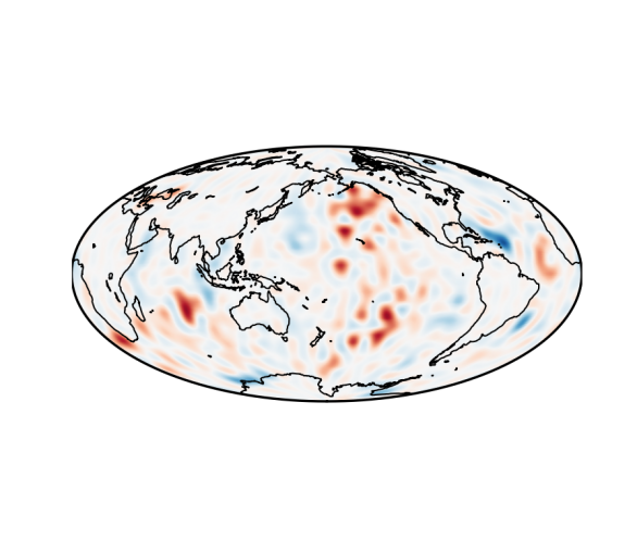
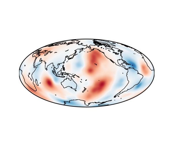
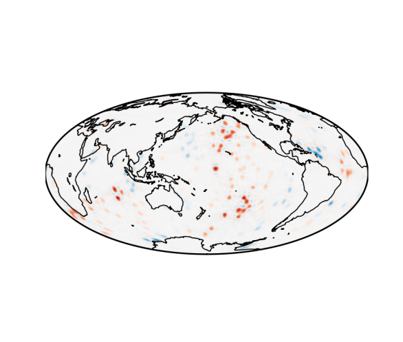
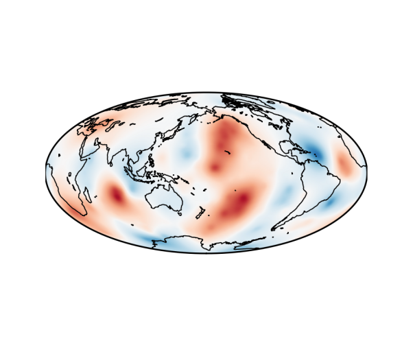
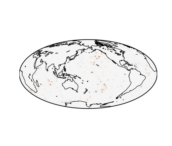
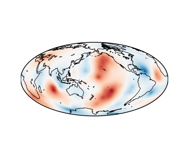
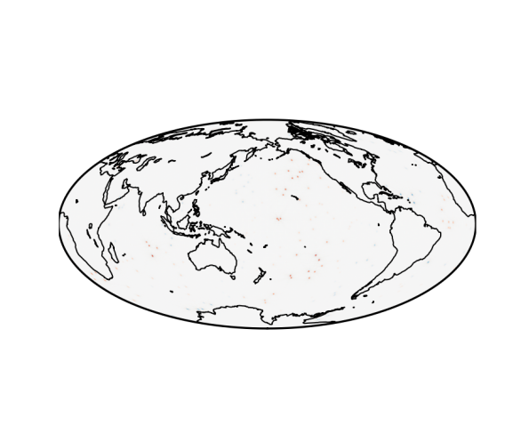
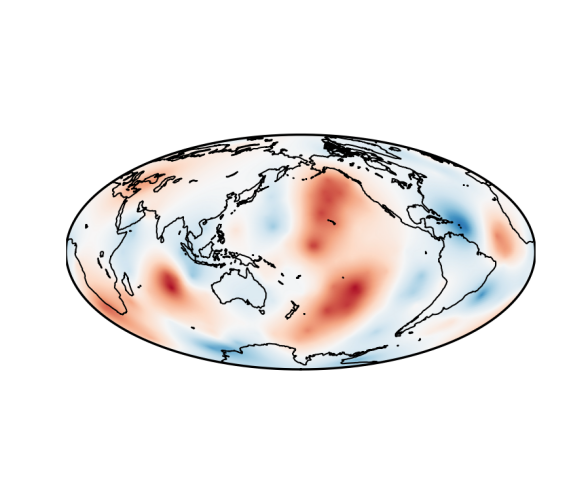
Figure 2: Minimum norm solutions at different truncation degrees obtained from the point data shown in Fig.1. For clarity data locations and values are not displayed, but in each case the point-values are fit to to within a relative error of $10^{-8}$. On the left hand side we show, in order from top to bottom, solutions obtained using an $L^{2}(\mathbb{S}^{2})$ formulation at truncation degrees $32$, $64$, $128$, and $256$. The right hand side then shows the analogous solutions calculated in $H^{s}(\mathbb{S}^{2})$ with $s=1.5$ and $\lambda=0.2$, and it is only in this case that pointwise convergence occurs.

From the inequality in eq.(104) we can see that the bounding hyperellipsoid has centre at $\tilde{w}$, and while its shape is determined by the positive-definite operator $B|_{\ker A}B|_{\ker A}^{*}$. To apply this result practically we first determine the property vector $\tilde{w}$ corresponding to the minimum norm solution of $v=Au$. We then calculate the components of the operator $B|_{\ker A}B|_{\ker A}^{*}$ which, using eq.(99), can be written

$$B|_{\ker A}B|_{\ker A}^{*}=B\,\mathbb{P}_{\ker A}B^{*}.$$ (107)

Computing the action of the property mapping or its adjoint is trivial, and so the main cost is associated with the orthogonal projection onto $\ker A$. Letting $\{g_{j}\}_{j=1}^{p}$ be a basis for $G$, we set $u_{j}=B^{*}g_{j}$ and $v_{j}=Au_{j}$. Recalling Corollary 2.4, it follows readily that

$$B\,\mathbb{P}_{\ker A}B^{*}g_{j}=B(u_{j}-\tilde{u}_{j}),$$ (108)

where $\tilde{u}_{j}$ is the minimum norm solution of $v_{j}=Au$. In this manner, we see that the bounding hyperellipsoid defined through eq.(104) can be determined at the cost of $\dim G+1$ minimum norm solutions.

Once the vector $\tilde{w}\in G$ and the operator $B|_{\ker A}B|_{\ker A}^{*}\in\mathrm{Hom}(G)$ have been calculated, it can be readily checked whether a given property vector $w\in G$ is consistent with eq.(104). For $\dim G\leq 2$ a graphical representation of this subset is trivial, but this cannot be done in higher-dimensions. It is, therefore, useful to determine the values obtained by a certain functional on $G$ as $w$ varies over the subset. As a simple example, we consider the linear functional $w\mapsto\left({w^{\prime}},{w}\right)_{G}$ for given $w^{\prime}\in G$. It is clear geometrically that this functional can be extremised subject to eq.(105) only when $w$ lies on the bounding hyperellipsoid. Applying the method of Lagrange multipliers (e.g. Luenberger, 1997) it is readily seen that the two stationary points occur at

$$w=\tilde{w}\pm\sqrt{\frac{r^{2}-\|\tilde{u}\|_{E}^{2}}{\left({B|_{\ker A}B|_{\ker A}^{*}w^{\prime}},{w^{\prime}}\right)_{G}}}B|_{\ker A}B|_{\ker A}^{*}w^{\prime},$$ (109)

and hence the functional’s minimum and maximum values are

$$\left({w^{\prime}},{w}\right)_{G}=\left({w^{\prime}},{\tilde{w}}\right)_{G}\pm\sqrt{(r^{2}-\|\tilde{u}\|_{E}^{2})\left({B|_{\ker A}B|_{\ker A}^{*}w^{\prime}},{w^{\prime}}\right)_{G}}.$$ (110)

A similar approach can be applied to non-linear functionals, though the optimisation problems become more complicated.

2.5.2 Application to the spectral estimation problem

Using eq.(222), point evaluation of a function in $H^{s}(\mathbb{S}^{2})$ can be written

$$u(x)=\left({\hat{\delta}_{x}},{u}\right)_{H^{s}(\mathbb{S}^{2})},$$ (111)

where $\hat{\delta}_{x}$ is the $H^{s}(\mathbb{S}^{2})$-representation of the Dirac measure at $x\in\mathbb{S}^{2}$. It follows that the data mapping can be written

$$Au=\sum_{i=1}^{n}\left({\hat{\delta}_{x_{i}}},{u}\right)_{H^{s}(\mathbb{S}^{2})}\,f_{i},$$ (112)

where $f_{1},\dots,f_{n}$ denote the standard basis vectors for the data space $\mathbb{R}^{n}$. The adjoint data mapping is given by

$$A^{*}v=\sum_{i=1}^{n}\left({f_{i}},{v}\right)_{\mathbb{R}^{n}}\,\hat{\delta}_{x_{i}}.$$ (113)

We write $\hat{Y}_{lm}$ for the $H^{s}(\mathbb{S}^{2})$-representation of the $(l,m)$th spherical harmonic functional

$$u\mapsto\int_{\mathbb{S}^{2}}u\,Y_{lm}\,\mathrm{d}S.$$ (114)

The property mapping is then given by

$$Bu=\sum_{j=1}^{p}\left({\hat{Y}_{l_{j}m_{j}}},{u}\right)_{H^{s}(\mathbb{S}^{2})}\,g_{j},$$ (115)

where $g_{1},\dots,g_{p}$ denote the standard basis vectors for the property space $\mathbb{R}^{p}$, while its adjoint is

$$B^{*}w=\sum_{j=1}^{p}\left({g_{j}},{w}\right)_{\mathbb{R}^{p}}\,\hat{Y}_{l_{j}m_{j}}.$$ (116)

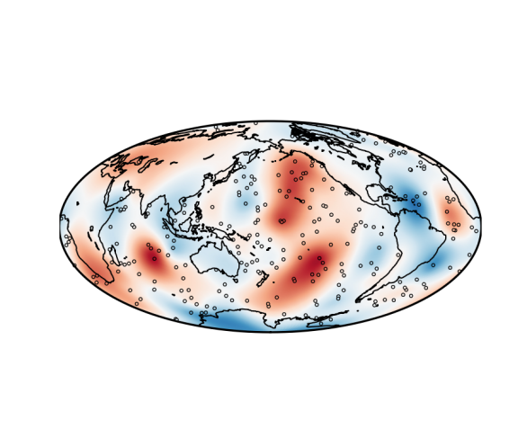
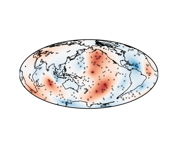
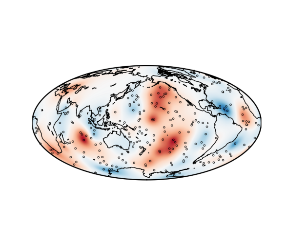
Figure 3: Minimum norm solutions obtained from the data in Fig.1 using different values for the Sobolev parameters. For the top left model the values used were $s=2.0$ and $\lambda=0.5$. For the top right model the values used were $s=1.1$ and $\lambda=0.5$. For the bottom left model the values used were $s=2.0$ and $\lambda=0.1$. For the bottom right model the values used were $s=1.1$ and $\lambda=0.1$. As a general trend, as either $s$ or $\lambda$ decrease the models become more localised about the observation points.

As discussed in Appendix B.5, within numerical calculations we make use of truncated spherical harmonic expansions, and hence replace the data mapping $A$ in eq.(112) with the following approximation

$$A_{L}u=\sum_{i=1}^{n}\left({\hat{\delta}_{x_{i},L}},{u}\right)_{H^{s}(\mathbb{S}^{2})}\,f_{i},$$ (117)

where $\hat{\delta}_{x,L}$ is the truncated $H^{s}(\mathbb{S}^{2})$-representation of a Dirac measure at degree $L$. Using eq.(233) it is readily shown that

$$\|A-A_{L}\|_{\mathrm{Hom}(H^{s}(\mathbb{S}^{2}),\mathbb{R}^{n})}\leq n\left(\sum_{l=L+1}^{\infty}\frac{2l+1}{4\pi}\left\langle{l}\right\rangle_{\lambda}^{-2s}\right)^{\frac{1}{2}},$$ (118)

where $\|\cdot\|_{\mathrm{Hom}(H^{s}(\mathbb{S}^{2}),\mathbb{R}^{n})}$ denotes the operator-norm defined in eq.(178). By taking the truncation degree sufficiently high, the term on the right hand side can be made as small as we wish, and hence minimum norm solutions obtained for the discretised problem converge to the correct model in $H^{s}(\mathbb{S}^{2})$ as the truncation degree is increased.

As a first example, we show why it is necessary to formulate inference problems using an appropriate function space. We noted above that $L^{2}(\mathbb{S}^{2})$ is not suitable for the problem at hand because elements of this space do not have well-defined point values. Once, however, things have been approximated using truncated spherical harmonic expansions, there is nothing to stop us calculating minimum norm solutions relative to the structure induced from $L^{2}(\mathbb{S}^{2})$. Moreover, so long as the truncation degree is sufficiently high, this approach yields models that fit the data to numerical precision. But as is seen in the left column of Fig.2, as the truncation degree is increased a sequence of models is obtained that does not converge in a pointwise sense. In stark contrast, the right hand column in Fig.2 shows the rapid convergence obtained from the same data when minimum norm solutions are sought within an appropriate choice of Sobolev space. For reference, these solutions were obtained using the gradient-based minimisation approach discussed above using the L-BFGS algorithm (e.g. Nocedal & Wright, 2006) coupled to the robust line search method of Moré & Thuente (1994). Moreover, the action of data and property mappings and their adjoints have been implemented in a matrix-free manner using fast spherical harmonic transformations. As a result, the method can be readily applied to situations involving high truncation degrees and/or large data sets.

Next we show in Fig.3 four minimum norm solutions obtained from the data in Fig.1 using different values of the Sobolev parameters $s$ and $\lambda$. In each case the truncation degree was taken sufficiently high that convergence has been achieved to a relative error less than $10^{-8}$. The differences between these results emphasises that minimum norm solutions depend on the inner product chosen for the model space, and hence none of these models has any particular interest. In fact, it is not difficult to show that any model that fits the data is the minimum norm solution relative to some compatible choice of inner product for the model space. The calculation of minimum norm solutions is simply a necessary step within the implementation of our broader theory once a suitable prior norm bound has been selected.

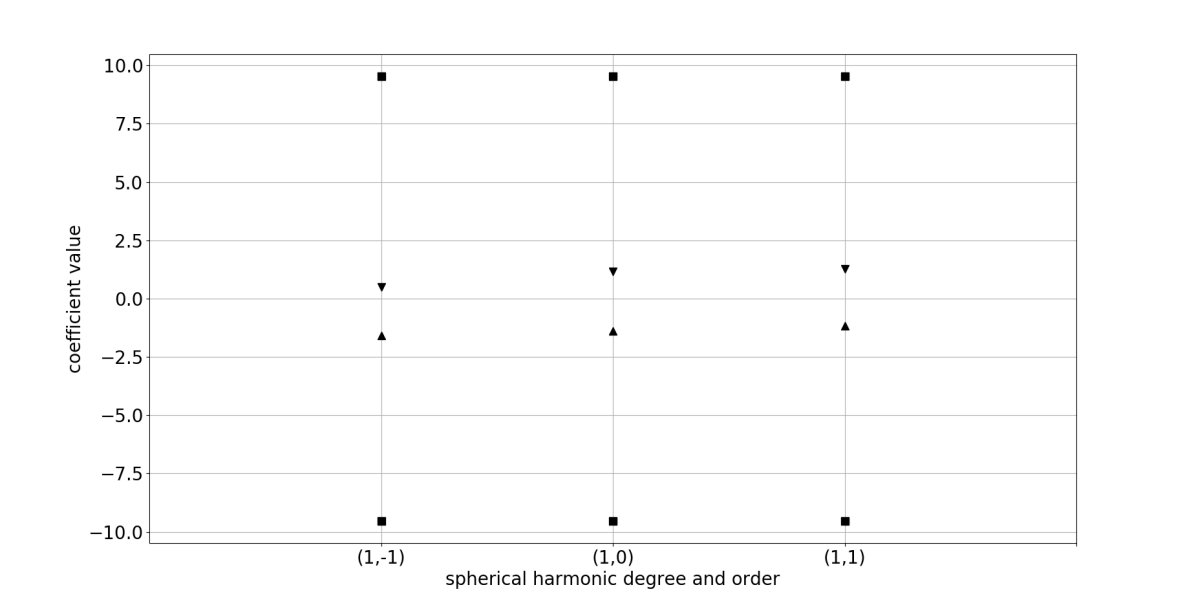
Figure 4: Limits on the degree one spherical harmonic coefficients obtained from the data shown in Fig.1 in conjunction with the prior norm bound $\|u\|_{H^{s}(\mathbb{S}^{2})}\leq\frac{5}{4}\|\tilde{u}\|_{H^{s}(\mathbb{S}^{2})}$ with $\tilde{u}$ the minimum norm solution, and Sobolev parameters $s=2$ and $\lambda=0.25$. For each coefficient the black squares indicate the limits placed by the prior norm bound, while the triangles show the smaller interval once the data is incorporated.

As our final example for this section we consider the implementation of eq.(104). Again, we use the data shown in Fig.1, and choose to work in the Sobolev space with $s=2$ and $\lambda=0.25$. A prior norm bound is required, and to insure compatibility with the data we take the radius of the constraint set to be

$$r=\frac{5}{4}\|\tilde{u}\|_{H^{s}(\mathbb{S}^{2})},$$ (119)

where $\tilde{u}$ is the minimum norm solution. In a real application such a norm bound would, of course, need to be carefully justified. As the property space we consider all degree $l=1$ spherical harmonic coefficients, and hence $\dim G=3$. The main cost of implementing eq.(104) is the calculation of $3+1$ minimum norm solutions. We show in Fig.4 the limits placed the individual coefficient obtained using eq.(110). The plot also shows permissible values using the prior constraint alone, and it can be seen that the data has substantially improved our knowledge of these coefficients. This situation contrasts markedly with the the behaviour of the problem when posed in $C^{0}(\mathbb{S}^{2})$, and substantiates our hope that the incorporation of derivative information into the model space topology would be useful. A limitation of Fig.4 is that trade-offs between the uncertainties in the coefficients cannot be seen. As a step towards doing this, we show in Fig.5 the pair-wise trade-offs between the different coefficients obtained using eq.(110). We finally show in Fig.6 the result obtained when the property space is expanded to comprise all coefficients of degree less than or equal to three. In this manner we see that relatively large property spaces can be handled, though the visualisation of the trade-offs between the coefficients becomes more challenging as $\dim G$ increases.

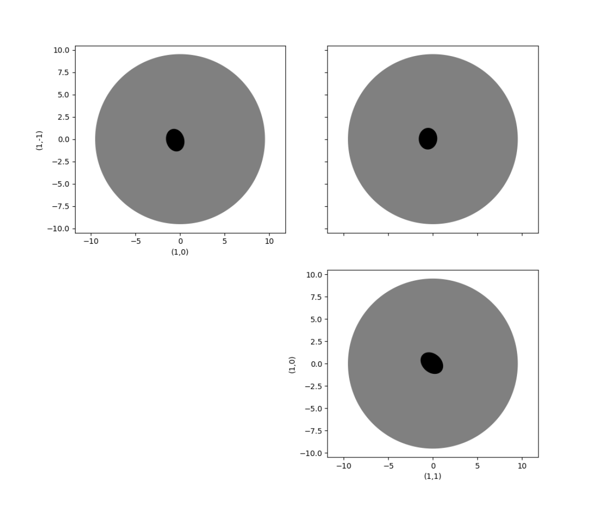
Figure 5: As for Fig.4, but here showing two-dimensional slices through the property space that indicate the pair-wise trade offs between the different coefficients. In each plot the axes are labelled with the degree and order of the coefficients considered. The gray shaded region then shows the limits placed by the prior norm bound, while the smaller black region is that resulting from the incorporation of the data.

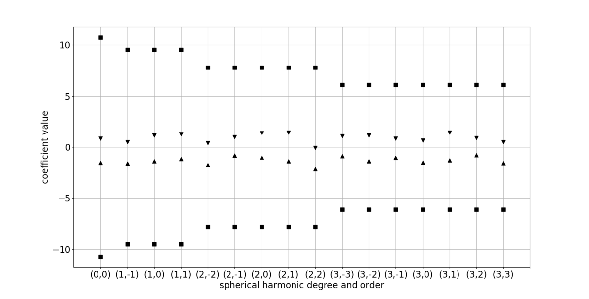
Figure 6: As for Fig.4, but now showing all spherical harmonic coefficients having degree $l\leq 3$.

2.6 Backus-Gilbert estimators

Prior to Backus’ independent work on inference problems a related but different approach was described by Backus & Gilbert (1967, 1968, 1970), with these ideas later being usefully adapted within the SOLA method of Pijpers & Thompson (1992, 1994). The extension of Backus-Gilbert estimators to Banach spaces has been discussed by Stark (2008), and here a broadly similar approach is used. For arbitrary $C\in\mathrm{Hom}(F,G)$ we can map the data $v=Au$ into the property vector $Cv=CAu$; in words, an estimate of the property vector is sought by forming appropriate linear combinations of the data. From Theorem 2.1 there is no $C$ such that $CA=B$, and hence the property vector cannot be recovered exactly. Nevertheless, if we can find $C$ such that $CA$ approximates $B$ suitably, then $Cv$ might still provide a useful estimate of the property vector. To proceed, for given $C\in\mathrm{Hom}(F,G)$ we set $\tilde{w}=Cv$, and write

$$w=\tilde{w}+Hu,$$ (120)

where $w$ is the true value of the property vector and $H=B-CA$. Noting that $H^{\prime}=B^{\prime}-A^{\prime}C^{\prime}$, the transversality assumption implies that $\ker H^{\prime}$ is trivial, and hence $H$ is surjective for any choice of $C$. It follows that the property vector can take any value in $G$ if no prior constraints are placed on the model. Indeed, this is just another way of proving Theorem 2.2. Assuming, therefore, that $u\in U$ for a given constraint set, the property vector satisfies

$$w\in\tilde{w}+HU=\{\tilde{w}+Hu\,|\,u\in U\}.$$ (121)

The validity of this result depends, of course, on $v=Au$ having solutions in $U$. Supposing that this holds, $\tilde{w}+HU$ and $BU$ have non-empty intersection, and hence the property vector is contained in

$$(\tilde{w}+HU)\cap BU,$$ (122)

which is bounded if the same is true of $\pi_{B}U$. Different choices of $C\in\mathrm{Hom}(F,G)$ lead to different estimates and, having quantified what constitutes a “good subset”, we could seek an optimal value for this linear mapping.

To proceed we assume for simplicity that $E$ is Hilbertable and that the prior constraint takes the form $u\in B_{r}(0)$ for some compatible choice of inner product. The image of the closed ball $B_{r}(0)$ under the affine mapping $u\mapsto\tilde{w}+Hu$ is a closed set whose boundary is a hyperellipsoid. Indeed, for a point $w$ in this set we have $w-\tilde{w}=Hu$ for some $u\in E$, and hence, using Proposition 2.5, we obtain

$$u=H^{*}(HH^{*})^{-1}(w-\tilde{w})+u_{0},$$ (123)

with $u_{0}\in\ker H$. But as $u\in B_{r}(0)$ it follows that

$$\left({(HH^{*})^{-1}(w-\tilde{w})},{w-\tilde{w}}\right)_{G}\leq r^{2}.$$ (124)

We would like this subset to be as small as possible, but what is meant by small in this context must be decided. When $\dim G=1$, the subset degenerates to an interval, and so we should clearly minimise its length. A simple extension of this idea is to consider the arithmetic average of the squared-lengths of the hyperellipsoid’s principle axes. We therefore seek $C\in\mathrm{Hom}(F,G)$ such that

$$J(C)=\mathrm{tr}[(B-CA)(B-CA)^{*}],$$ (125)

is minimised. Differentiating and setting the result equal to zero, the optimal linear estimator is readily found to be

$$C=BA^{*}(AA^{*})^{-1}.$$ (126)

Recalling Proposition 2.5, $\tilde{w}=Cv$ is exactly what would be obtained from the minimum norm solution of $v=Au$. Moreover, we have

$$H=B-CA=B[1-A^{*}(AA^{*})^{-1}A]=B\,\mathbb{P}_{\ker A},$$ (127)

which, using eq.(99), implies that

$$HH^{*}=B\,\mathbb{P}_{\ker A}B^{*}=B|_{\ker A}B|_{\ker A}^{*}.$$ (128)

The optimal Backus-Gilbert estimator, therefore, leads to the following restriction on the property vector

$$\left({(B|_{\ker A}B|_{\ker A}^{*})^{-1}(w-\tilde{w})},{w-\tilde{w}}\right)_{G}\leq r^{2},$$ (129)

which is identical to eq.(104) but for the lack of a term on the right hand side associated with the minimum norm value. This absence makes perfect sense because the optimality condition in eq.(125) is defined without reference to the data. As a consequence Backus-Gilbert estimators will generically overestimate uncertainty relative to applications of Backus’ later theory.

3 Linear inference problems with data errors

In this section we show how our previous results can be extended to account for random data errors. While most ideas apply to problems with Banachable model spaces, the practical implementation of the method again only seems feasible if an appropriate Hilbert space structure can be introduced. It is worth emphasising that our discussion is not limited to the case of Gaussian errors, with a wide range of unimodal distributions being accommodated at little to no additional cost. Broadly similar methods can be applied in the context of Backus-Gilbert estimators, and these are discussed briefly at the end of the section.

3.1 Formulation of the problem

The vector spaces and operators introduced in Section 2.1 carry over directly. The surjectivity condition on the data mapping will, however, be dropped to allow for data-redundancy. Instead we require the following:

Assumption 3.1

The property mapping is surjective, while the transversality condition $\mathrm{im}A^{\prime}\cap\mathrm{im}B^{\prime}=\{0\}$ holds.

To account for data errors, we generalise the relationship between the unknown model $u\in E$ and the observed data $v\in F$ to

$$v=Au+z,$$ (130)

where $z$ is a realisation of an $F$-valued random variable. The probability distribution from which the error term is drawn will be denoted by $\nu$ and is assumed to be known exactly. The data is, therefore, a realisation of a random variable whose probability distribution is determined by $\nu$ along with the unknown value $Au$. As ever, the inference problem aims to use the data to constrain the value of the property vector $w=Bu$ subject to the model satisfying $u\in U$ for a given constraint set $U\subseteq E$.

The data $v\in F$ does not now tell us $Au$ directly, and we must use our knowledge of $\nu$ to determine which values for $Au$ are plausible. We seek an approach that would be infrequently wrong under hypothetical repetitions, taking this behaviour as characteristic of a sound statistical procedure – see Mayo (2018) for an interesting and nuanced discussion of such issues. To this end, we define a confidence set for $\nu$ having a confidence level, $1-\alpha$, as a subset $V\subseteq F$ such that

$$\nu(V)=1-\alpha,$$ (131)

with $\alpha\in[0,1]$. The interpretation is simply that if realisations are repeatedly drawn from $\nu$, the results will lie in $V$ with a relative frequency that tends to the confidence level. For a given distribution there will generally be many different confidence sets having the same confidence level, and additional criteria must be invoked to single out one of practical interest. Nonetheless, having fixed an appropriate choice of $V\subseteq F$, for each realisation $v$ of the data we know that $z=v-Au$ is a realisation of the random error, while the condition $v-Au\in V$ is equivalent to $Au\in v-V$. It follows that whatever the true value of $u$, if, hypothetically, the data generated from this model could be observed many times, then the relative frequency at which $Au\in v-V$ holds would tend to $1-\alpha$. From the data $v\in F$ we, therefore, choose to infer that $Au\in v-V$. This may, of course, be incorrect in any given instance, but such is the nature of statistics.

An appealing feature of this approach is that deterministic errors in the data mapping can, in principle, be incorporated with relative ease. Suppose that $a:E\rightarrow V$ denotes the exact (and possibly non-linear) data mapping, and hence eq.(130) should be replaced by

$$v=a(u)+z.$$ (132)

If $A\in\mathrm{Hom}(E,F)$ is the linear and approximate data mapping to be used, then we can write

$$v=Au+[a(u)-Au]+z.$$ (133)

Let us assume there is a bounded subset $V_{d}\subseteq F$ such that

$$a(u)-Au\in V_{d},$$ (134)

for all models $u$ within the constraint set $U\subseteq E$. Adapting the above argument, it follows that from the observed data $v\in F$ we can conclude that $Au\in v-V^{\prime}$ where $V^{\prime}=V+V_{d}$ may be viewed as a modified confidence set. Here, of course, we see the familiar idea that theoretical uncertainties can be pragmatically addressed by increasing the magnitude of the random data errors.

3.2 Generalising Backus’ theorems

Our aim is to determine the property vector $w=Bu$ as best possible from the information $u\in U$ and $Au\in v-V$, where $U\subseteq E$ a constraint set for the model, and $V\subseteq F$ a confidence set for the data error. Given that the data mapping need not be surjective, the observed data $v\in F$ may not belong to $\mathrm{im}A$. For example, suppose that the distribution $\nu$ has a probability density function $p:V\rightarrow\mathbb{R}$ relative to a volume measure $\mathrm{d}v$ on $F$ such that

$$\nu(V)=\int_{V}p(v)\,\mathrm{d}v$$ (135)

for any subset $V\subseteq F$. If $\mathrm{im}A$ is a proper subspace of $F$ it has zero-volume, and so

$$\nu(\mathrm{im}A)=0,$$ (136)

which is to say that the observed data will almost surely lie outside of the image of the data mapping. It is worth noting that such a probability density function need not always exist. For example, the error free-case can be recovered by taking $\nu$ to be a Dirac measure at the origin. In any case, what really matters is that

$$(v-V)\cap\mathrm{im}A\neq\emptyset,$$ (137)

this meaning that there exist models that fit the observed data in a statistically acceptable manner.

To allow for $A$ to be non-surjective, the factorisation of the data mapping in eq.(49) is readily generalised to

$$A=i_{\mathrm{im}A}\,\hat{A}\,\pi_{A},$$ (138)

where $\pi_{A}$ is the quotient mapping onto $E/\ker A$, $\hat{A}\in\mathrm{Hom}(E/\ker A,\mathrm{im}A)$ is continuously invertible, and $i_{\mathrm{im}A}\in\mathrm{Hom}(\mathrm{im}A,F)$ is the inclusion mapping (e.g. Treves, 1967, Proposition 4.6). For each point $\tilde{v}\in(v-V)\cap\mathrm{im}A$ we can associate a closed affine subspace $\pi_{A}^{-1}\{\hat{A}^{-1}\tilde{v}\}$ within the model space. Making use of Assumption 3.1, the proof of Theorem 2.2 is then readily generalised to show that for any $\tilde{v}\in(v-V)\cap\mathrm{im}A$ and $w\in G$ there are infinitely many models such that $Au=\tilde{v}$ and $Bu=w$. Thus, as must be expected, the incorporation of data errors does nothing to lessen the need for prior constraints within the inference problem. Using eq.(138) we see that the subset

$$U_{v-V}=\pi_{A}^{-1}\hat{A}^{-1}[(v-V)\cap\mathrm{im}A],$$ (139)

contains all models that fit the data in a statistical sense. The data is, therefore, compatible with the prior constraint $u\in U$ if and only if $U\cap U_{v-V}$ is non-empty, this result generalising the first part of Theorem 2.3. To extend the second part of that theorem, we use eq.(51) to conclude that $B(U\cap U_{v-V})$ is bounded if and only if the same is true of $\pi_{B}(U\cap U_{v-V})$. For later reference, we note that if the constraint set $U$ and the confidence set $V$ are convex, then the same is true of $B(U\cap U_{v-V})$, this following because the intersection of two convex sets is convex, while convexity is preserved under images and inverse images of linear mappings. Finally, the discussion in Section 2.4 on the relationship between prior constraints and the choice of model space carries over unchanged.

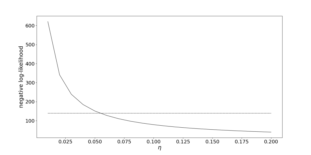
Figure 7: A graphical illustration of how eq.(149) can be solved. For each value of $\eta>0$ we solve a convex optimisation problem associated with the function $u\mapsto J(u,\eta)$ defined in eq.(147), and the plot shows the negative log-likelihood for the models so obtained. The dashed line indicates the squared-radius of the desired confidence set, and the intersection of these curves gives the value of $\eta$ corresponding to the model with smallest norm that fits the data in a statistically acceptable fashion. These calculations were done for the data set shown in Fig.1 but with uncorrelated Gaussian errors added to each datum as described in Section 3.3.2. The confidence set is that defined in eq.(142) with confidence level $0.9$, while Sobolev parameters $s=2$ and $\lambda=0.25$ were selected.

3.3 Implementation in Hilbert spaces

3.3.1 General theory

We assume that $E$ is Hilbertable and that the constraint set takes the form $u\in B_{r}(0)$ relative to a compatible choice of inner product. Balls not centred at the origin are readily handled by translation. Using an orthonormal basis, we can establish an isomorphism between $F$ and $\mathbb{R}^{n}$. On the latter space we have the usual Lebesgue measure, and this can be trivially pulled-back to a translation-invariant volume measure $\mathrm{d}v$ on $F$ which is independent of the choice of orthonormal basis. To define a suitable confidence set, let us suppose that $\nu$ can be expressed in terms of a probability density function $p:F\rightarrow\mathbb{R}$ relative to $\mathrm{d}v$ which takes the form

$$p(v)=a\,\mathrm{e}^{-l(v)},$$ (140)

where $a$ is a normalisation constant and $l:F\rightarrow\mathbb{R}$ is known as the negative log-likelihood. We assume that $l$ is non-negative, continuously differentiable and strictly convex. One example is the ubiquitous Gaussian distribution which has

$$l(v)=\frac{1}{2}\left({R^{-1}(v-\bar{v})},{v-\bar{v}}\right)_{F},$$ (141)

where the covariance $R\in\mathrm{Hom}(V)$ is self-adjoint and positive-definite, and $\bar{v}$ is the expectation. For such distributions, a sensible and convenient choice of confidence set is defined in terms of the negative log-likelihood by

$$V=\{v\in F\,|\,l(v)\leq s^{2}\},$$ (142)

where $s>0$ is fixed uniquely by the requirement that the confidence level $1-\alpha$ be met. Because $l$ is continuous and strictly convex, it follows that $V$ is a closed and convex set. The boundary of the confidence set is, by definition, equal to the inverse image

$$\partial V=l^{-1}(\{s^{2}\}).$$ (143)

As a final assumption, we require that the derivative $Dl:V\rightarrow V^{\prime}$ is nowhere vanishing on $\partial V$ and hence, by the regular value theorem (e.g Spivak, 1970), this boundary is a closed submanifold in $F$ with a continuous outward unit normal vector field. It is worth emphasising that these conditions on $p$ hold for a wide range of unimodal distributions, and not only for the Gaussian distribution.

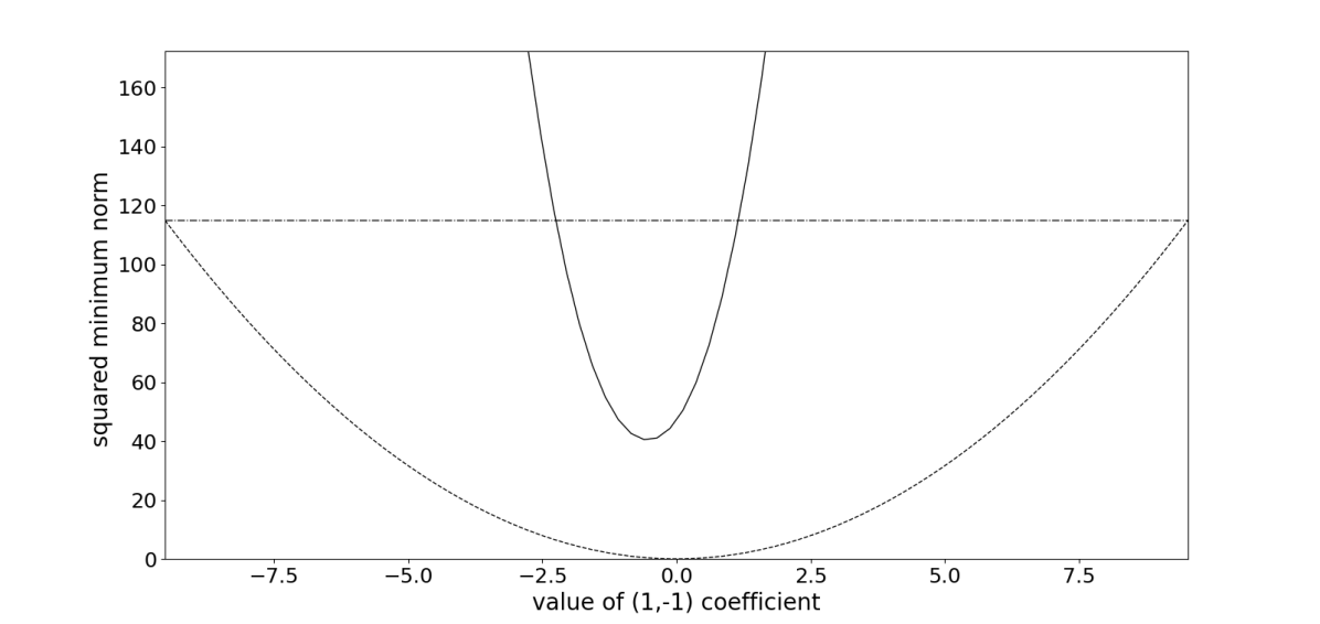
Figure 8: An illustration of how bounds are placed on a component of the property vector, with the data, confidence set, and model space parameters as described in Fig. 7. The horizontal dot-dashed line shows the squared-value of the prior norm bound, this being equal to that used in the error-free case shown in Figs. 4, 5, and 6. The dashed curve then shows the squared minimum norm value for a model whose $(1,-1)$ spherical harmonic coefficient is given by the ordinate, while the solid curve shows the corresponding value when the model is also required to fit the data in a statistically acceptable sense. The intersections between dashed and dot-dashed curves gives the interval in which the prior constraint requires the $(1,-1)$ coefficient to lie, while the smaller interval defined by the intersections of the solid and dot-dashed curves shows what happens once the data is used.

Given these preliminaries, we first consider how the compatibility of the prior constraint with the data can be established. To this end we define $U_{v-V}=A^{-1}(v-V)$ and wish to determine whether its intersection with the constraint set $B_{r}(0)$ is non-empty. A necessary and sufficient condition for this to hold is given by

$$\inf_{u\in U_{v-V}}\|u\|_{E}\leq r.$$ (144)

Note that, by definition, the infimum of an empty set of real numbers is equal to positive infinity, and hence this condition is meaningful even if $U_{v-V}$ is empty. Supposing for the moment that $U_{v-V}$ is non-empty, we know that this set is closed and convex. The general form of the projection theorem in Hilbert spaces (e.g. Treves, 1967, Theorem 12.1) shows that there is a unique point in $U_{v-V}$ such that the infimum value of the norm is attained. If $0\in U_{v-V}$ then the infimum vanishes, and eq.(144) is trivially satisfied. Otherwise it is clear geometrically that the unique minimum lies somewhere on the boundary $\partial U_{v-V}$. In terms of the negative log-likelihood we have

$$U_{v-V}=\{u\in E\,|\,l(v-Au)\leq s^{2}\},$$ (145)

and noting that $u\mapsto l(v-Au)$ is convex, it follows that

$$\partial U_{v-V}=\{u\in E\,|\,l(v-Au)=s^{2}\}.$$ (146)

Applying the Lagrange multiplier theorem (e.g. Luenberger, 1997), we are led to introduce the functional

$$J(u,\eta)=\frac{1}{2}\|u\|_{E}^{2}+\eta\left[l(v-Au)-s^{2}\right],$$ (147)

such that desired minimum can be obtained by solving the simultaneous equations

$$D_{u}J(u,\eta)=0,\quad D_{\eta}J(u,\eta)=0,$$ (148)

which take the concrete form

$$u-\eta\,A^{*}\mathscr{J}_{F}Dl(v-Au)=0,\quad l(v-Au)-s^{2}=0,$$ (149)

where we recall that $\mathscr{J}_{F}\in\mathrm{Hom}(F^{\prime},F)$ is defined through the Riesz representation theorem. If $u$ is the unique minimum point, then the first equation can be interpreted geometrically as saying that from this point on $\partial U_{v-V}$ we can reach the origin by moving a signed distance $\eta$ along the boundary’s outward unit normal. By assumption $U_{v-V}$ is disjoint from the origin, and hence $\eta$ must be positive. Moreover, for each fixed $\eta>0$ the first equation defines the unique minimum point of the convex functional $u\mapsto J(u,\eta)$. In this manner, the above set of non-linear equations can be reduced to root-finding in a single positive real variable. Indeed, for fixed $\eta>0$, we can apply gradient-based methods to uniquely solve the convex optimisation problem for $u$. The result may then be substituted into the second part of eq.(149) to check if the constraint is met. In considering this root finding problem the following is useful:

Lemma 3.1

Let $u_{\eta}$ denote the unique minimum point of $u\mapsto J(u,\eta)$ for fixed $\eta>0$. The function

$$\eta\mapsto l(v-Au_{\eta}),$$ (150)

is non-increasing for all $\eta>0$.

Proof: Differentiating $\eta\mapsto l(v-Au_{\eta})$ we obtain

$$\frac{\mathrm{d}}{\mathrm{d}\eta}l(v-Au_{\eta})=-\left({A^{*}\mathscr{J}_{F}\,Dl(v-Au_{\eta})},{u_{\eta}^{\prime}}\right)_{E},$$ (151)

where $u^{\prime}_{\eta}=\frac{\mathrm{d}u_{\eta}}{\mathrm{d}\eta}$. Next by implicitly differentiating the first identity in eq.(149) we find

$$\left[1+\eta A^{*}\mathscr{J}_{F}D^{2}l(v-Au_{\eta})A\right]u^{\prime}_{\eta}=A^{*}\mathscr{J}_{F}Dl(v-Au_{\eta}).$$ (152)

Because the negative log-likelihood is strictly convex, its Hessian $D^{2}l(v)\in\mathrm{Hom}(F,F^{\prime})$ is symmetric and positive-definite at each point. It follows that the linear operator on the left-hand side is also positive-definite, and hence we obtain

$$u^{\prime}_{\eta}=\left[1+\eta A^{*}\mathscr{J}_{F}D^{2}l(v-Au_{\eta})A\right]^{-1}A^{*}\mathscr{J}_{F}Dl(v-Au_{\eta})=\frac{1}{\eta}\left[1+\eta A^{*}\mathscr{J}_{F}D^{2}l(v-Au_{\eta})A\right]^{-1}u_{\eta}.$$ (153)

Substituting into eq.(151) we then have

$$\frac{\mathrm{d}}{\mathrm{d}\eta}l(v-Au_{\eta})=-\frac{1}{\eta^{2}}\left({u_{\eta}},{\left[1+\eta A^{*}\mathscr{J}_{F}D^{2}l(v-Au_{\eta})A\right]^{-1}u_{\eta}}\right)_{E},$$ (154)

which shows that the derivative is non-positive.

$\blacksquare$

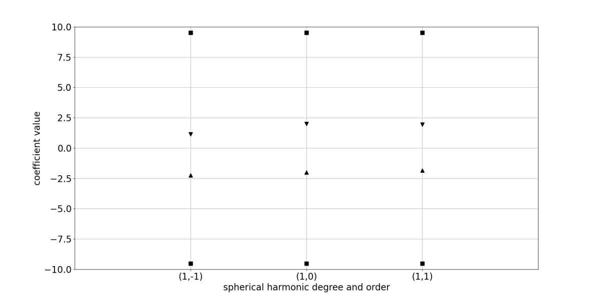
Figure 9: As for Fig.4, but showing constraints on the degree one coefficients once data errors are considered. For these calculations the Sobolev space parameters and prior norm bound were taken equal to those used in the error-free case, while a confidence level of $0.9$ was selected.

It follows that as $\eta$ tends to infinity the value of $l(v-Au_{\eta})$ approaches a positive lower bound which might be larger than $s^{2}$. In such a case there is no value of $\eta>0$ for which the second part of eq.(149) holds, this occurring precisely when $\mathrm{im}A\cap(v-V)$ is empty. The above method also, therefore, provides a constructive means for checking the validity of this assumption. It is interesting to note that the constrained optimisation problem associated with eq.(147) is identical in form to that within the Occam’s inversion of Constable et al. (1987). In the present context, however, the model obtained has no intrinsic value nor interest.

Suppose that, by the above method, we have verified that the constraint and data are compatible in the stated statistical sense. We then wish to know whether a given property vector $w\in G$ is consistent with both the constraint and data. For a fixed property vector $w\in G$, Proposition 2.5 shows that we must restrict attention to model vectors of the form

$$u=\tilde{u}+u_{0},$$ (155)

where $\tilde{u}=B^{*}(BB^{*})^{-1}w$ and $u_{0}\in\ker B$. The condition $u\in B_{r}(0)$ then implies $u_{0}\in B_{r_{0}}(0)\subseteq\ker B$ where we have set

$$r_{0}^{2}=r^{2}-\|\tilde{u}\|^{2}_{E},$$ (156)

this radius being well-defined if and only if $w$ is compatible with the prior constraint. Similarly, the inclusion $Au\in v-V$ is equivalent to $A|_{\ker B}u_{0}\in v_{0}-V$ where $v_{0}=v-A\tilde{u}$. This new problem is of exactly the same form as the one just solved. To work practically within the subspace $\ker B$ all that must be done is to replace each occurrence of the adjoint operator $A^{*}$ by

$$A|_{\ker B}^{*}=\mathbb{P}_{\ker B}A^{*},$$ (157)

with this identity being obtained by analogy with eq.(99).

To conclude this discussion, we note that as both the constraint set and confidence set are convex, the same is true of the subset of acceptable property vectors. While the above method shows how the inclusion of a vector $w\in G$ within this subset can be established, it has not led to a simple method for delimiting the subset’s boundary. This contrasts with the error-free case in Section 2.5 where the boundary was shown to be a hyperellipsoid that could be readily calculated. In fact, for each point $\tilde{v}\in\mathrm{im}A\cap(v-V)$, the method of Section 2.5 could be applied using the surjective mapping $\hat{A}\,\pi_{A}\in\mathrm{Hom}(E,\mathrm{im}A)$ defined through eq.(138), and would lead to a subset in $G$ with hyperellipsoidal boundary comprising some of the property vectors that are compatible with both the data and prior constraint. Taking the union of these subsets as $\tilde{v}$ ranges over $\mathrm{im}A\cap(v-V)$ we would arrive at the subset containing all acceptable property vectors. Looking back at eq.(104), we note that as $\tilde{v}$ varies the size and centre of the hyperellipsoids change, but not their shape nor orientation. Nevertheless, a union of such subsets cannot, in general, be expected to take any simple geometric form.

3.3.2 Application to the spectral estimation problem

To apply these ideas practically, we must first specify a probability distribution $\nu$ for the random data errors. For simplicity $\nu$ was taken to be a Gaussian distribution with diagonal covariance matrix and vanishing expectation. The standard deviation at each measurement location was drawn randomly from $[0.05,0.2]$ using a uniform distribution, with these errors lying between two and ten percent of the underlying functions maximum absolute value. Having specified the distribution, a confidence level of $0.9$ was selected, and the radius $s$ of the confidence set determined according to eq.(142). In the case of Gaussian errors, this can be done using the chi-squared statistic. More generally, random samples can be drawn from the distribution $\nu$ and used to determine an empirical cumulative distribution function for the random variable $v\mapsto l(v)$ from which the appropriate value of $s$ is trivially found.

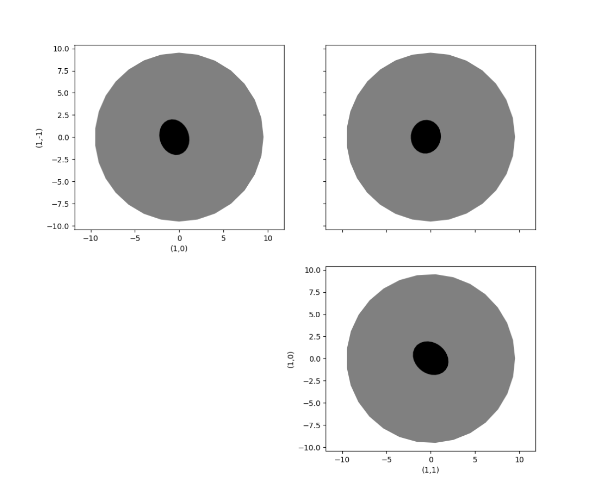
Figure 10: As for Fig.5, but showing constraints on the degree one coefficients once data errors are considered. For these calculations the Sobolev space parameters and prior norm bound were taken equal to those used in the error-free case, while a confidence level of $0.9$ was selected.

In Fig.7 we illustrate graphically the root finding required to solve the optimality condition in eq.(149). For each value of $\eta>0$, the function $u\mapsto J(u,\eta)$ can be minimised using a slight variant of the gradient-based methods applied in the error-free case. Notably, in this case the optimisation problem has a unique minimum, and hence the initial value within the iterative process does not matter. In particular, once we have solved the problem for a certain value of $\eta$, we could use this solution as the initial guess for a different but nearby $\eta$, and hence improve the efficiency of the method. In doing all this we need to fix the Sobolev parameters, and in this example the values $s=2$ and $\lambda=0.25$ were selected. The figure then shows the variation of the minimum value of the negative log-likelihood as a function of $\eta$, and it can be seen that the second equality in eq.(149) is satisfied for a suitable value of the argument. In practice, of course, this root is not found graphically, but obtained using a bisection algorithm.

As explained above, minimum norm solutions subject to given constraints on the property vector can be obtained in a near identical manner. For a given value of the property vector we can, therefore, determine the minimum norm value for the model that satisfies this constraint and fits the data in a statistical sense. If this norm value lies below the prior norm bound, the property vector is accepted, and if not, it is ruled out. An example of this process can be seen within Fig.8. Here the property space comprises just the $(1,-1)$ spherical harmonic coefficient, and we plot the variation of the squared minimum norm associated with different values of this coefficient. The horizontal dot-dashed line shows the squared-value of the chosen prior norm bound, and hence the interval in which the $(1,-1)$ coefficient must lie is delineated. Again, in practice, this interval is more efficiently determined using a bisection method. In Fig.9 we show the bounds obtained on each of the degree one spherical harmonic coefficients through this process. To aid in comparison with the earlier results, the prior norm bound was taken to have the same value as in the error free-case.

From a computational point of view it is worth emphasising that the incorporation of data errors comes at a fairly substantial cost. This is because the property vector no longer lies within an hyperellipsoidally bounded region, and hence a larger number of constrained optimisation problems must be solved to determine its form. This is especially true if simultaneous bounds on multiple directions in property space are sought as shown in Fig.10. There is, however, scope for making this process more efficient. For example, bounds along different directions in the property space are independent of one another, and hence the process can be trivially parallelised.

3.4 Incorporating data errors into Backus-Gilbert estimators

To conclude this section we show how data errors can be handled in the context of Backus-Gilbert estimators. While the resulting theory is less general and less precise than that just discussed, it is easier to implement numerically and so might sometimes be preferred. There are also interesting links with the probabilistic methods to be developed in the sequel; see Valentine & Sambridge (2020a, b) discussion of some related ideas. Starting with the general case, we use eq.(130) to write the property vector, $w=Bu$, in the form

$$w=\tilde{w}+Hu+Cz,$$ (158)

for an arbitrary $C\in\mathrm{Hom}(F,G)$, where $\tilde{w}=Cv$, and $H=B-CA\in\mathrm{Hom}(E,G)$. As previously, we introduce a constraint set, $U\subseteq E$, and a confidence set, $V\subseteq F$, and hence obtain the inclusion

$$w\in(\tilde{w}+HU+CV)\cap BU.$$ (159)

Different values of $C\in\mathrm{Hom}(E,F)$ lead to different bounds on the property vector, and so having decided what constitutes a good subset, we can seek to optimise the choice of this linear mapping.

To illustrate how this can be done practically we restrict attention to Hilbertable problems, take the constraint set to be $B_{r}(0)$ for some $r>0$, and assume Gaussian errors with zero expectation and covariance $R\in\mathrm{Hom}(F)$. The confidence set in eq.(142) can then be used, and comprises those data vectors for which

$$\frac{1}{2}\left({R^{-1}v},{v}\right)_{F}\leq s^{2},$$ (160)

where $s>0$ is fixed by the confidence level. As shown earlier, the image of the closed ball $B_{r}(0)$ under the affine mapping $u\mapsto\tilde{w}+Hu$ is a closed set in $G$ with hyperellipsoidal boundary whose elements satisfy

$$\left({(HH^{*})^{-1}(w-\tilde{w})},{w-\tilde{w}}\right)_{G}\leq r^{2}.$$ (161)

Similarly, the image of the confidence set under $v\mapsto Cv$ is a closed set in $G$ with hyperellipsoidal boundary whose elements satisfy

$$\frac{1}{2}\left({(CRC^{*})^{-1}w},{w}\right)_{G}\leq s^{2}.$$ (162)

The property vector lies in the sum of these two subsets, but in general the result will not have a hyperellipsoidal boundary. Nonetheless, because we want this subset to be suitably small, a reasonable quantity to minimise is

$$J(C)=r^{2}\,\mathrm{tr}[(B-CA)(B-CA)^{*}]+2s^{2}\,\mathrm{tr}[CRC^{*}],$$ (163)

which is proportional to the sum of the squared-lengths of the principle axes for the two hyperellipsoids. A simple calculation then shows that the chosen functional has a unique minimum at

$$C=BA^{*}\left(AA^{*}+2s^{2}r^{-2}R\right)^{-1},$$ (164)

which generalises eq.(126). Importantly, the inclusion of the data covariance guarantees that the inverse operator on the right hand side exists even if the data mapping fails to be surjective. To apply this method practically, we need only repeatedly act $\left(AA^{*}+2s^{2}r^{-2}R\right)^{-1}$ on data vectors, and this can be readily done either directly when $\dim F$ is small, or using standard iterative methods such as conjugate gradients. In total, this inverse operator needs to be acted $4\dim G+1$ times. The first is to find $\tilde{w}=Cv$, while $2\dim G$ further actions are required for the components of either $HH^{*}$ and $CRC^{*}$. This cost is around twice that of the error-free case, and is likely to be substantially less than that required for the Backus estimates discussed above.

4 Discussion

4.1 Summary of the main ideas

In spite of the technicality of this paper, the essential ideas are rather simple. Within an inference problem we are given data that have been produced from an unknown model. From this data we then wish to infer some other numerical properties of the model. In almost all cases the data alone will not be sufficient to place constraints on the property vector, and hence some form of prior constraint on the model must be assumed. Within this work we have considered only deterministic constraints, which is to say that the model is assumed to lie within a certain subset of the model space. With the prior constraint in place, we can first ask whether there exist models within the constraint set that fit the data in a statistically plausible manner. If the answer is no, then there is likely something wrong with either the prior constraint or the physical formulation of the problem. Assuming that there are models compatible with both the data and the prior constraint, we can proceed to test different values of the property vector as follows. We select a property vector of interest, and restrict attention to models for which this value is obtained. We then ask whether it is still possible to fit the data subject to the prior constraint. If it is, then we accept the value of the property vector, and if not we reject it as being inconsistent with our information. Repeating this process for different choices of property vector, we can delineate the region of the property space in which the true value must lie. It is worth emphasising that this general philosophy depends in no way on the inference problem being linear, and so applies equally well to non-linear problems. It is also important to note that though models are built within this process using methods similar to those for the solution of inverse problems, this is only as an intermediate step, and these models have no intrinsic interest.

To implement the theory, the main task is determining whether models exist that fit the data subject to given constraints; both prior and those imposed in testing a particular value for property vector. Doing this requires the solution of constrained optimisation problems, and it is here that great care is required. In the situation considered in most detail within this paper, the prior constraint took the form of a norm bound. To proceed, we sought the minimum norm value for models consistent with the constraints imposed by both the data and the property vector being tested. If the minimum norm value was smaller than the assumed bound, the property vector was accepted, and if not it was rejected. Thus, if the correct minimum norm value is not obtained within our calculations, we might reject viable property vectors or accept those that are not. It was to avoid this possibility that detailed mathematical analysis was necessary, with, in particular, the problem being posed on an appropriate function space, and the numerical methods being shown to be convergent. It is worth emphasising that in these optimisation problems it is only the minimum value of the functional that is of interest, and not whether this value is obtained by a unique model. Within linear inference problems it has been shown that this condition is always met, but this need not be so within non-linear problems.

The need to work in practice within Hilbert spaces requires some comment. As noted earlier, most geophysical inference problems are naturally posed on Banachable spaces, and it is also in such spaces that prior constraints are likely to be expressed. For example, with parameters like density or seismic wave speed we are far more likely to have information on the magnitude of their point-values and not on their norms in some exotic sounding Hilbert space. While the general theory has been developed on such Banachable spaces, we are quickly led to optimisation problems that are not tractable numerically. The move to Hilbert spaces is, therefore, done pragmatically, but Section 2.4 showed that this step can be rigorously justified so long as the prior constraints take a suitable form. An important practical question is the extent to which different types of prior information can be converted into a norm bound in a suitable Hilbert space. To give an indication of how this might be done, we return, as ever, to our motivating spectral estimation problem. In this case, suppose that we believe that the function is continuously differentiable and have the following bound on its point values

$$\|u\|_{C^{0}(\mathbb{S}^{2})}\leq r,$$ (165)

for some $r>0$. The Sobolev embedding theory tells us that $H^{s}(\mathbb{S}^{2})$ for $s>2$ is comprised of continuously differentiable functions, while using eq.(226) we can bound the supremum norm of its elements in terms of their Sobolev norm. It follows that the space $H^{s}(\mathbb{S}^{2})$ for $s>2$ along with the prior norm bound

$$\|u\|_{H^{s}(\mathbb{S}^{2})}\leq\left(\sum_{l\in\mathbb{N}}\frac{2l+1}{4\pi}\left\langle{l}\right\rangle_{\lambda}^{-2s}\right)^{-\frac{1}{2}}\,r,$$ (166)

provides a Hilbert space setting for the problem consistent with our prior information. The estimate within eq.(227) can be similarly applied in cases where pointwise bounds on the functions derivatives are also given. Clearly the passage to this Hilbert space is not free from ambiguity, with, for example, the values of $s$ nor $\lambda$ fixed in the above discussion. Moreover, Sobolev embeddings are strict, and so there will exist viable models that have been removed from the constraint set. Until, however, suitable progress is made with computational optimisation in Banach spaces, a certain amount of pragmatism is required.

4.2 Extensions and applications

To conclude it is worth commenting briefly on possible extensions and applications of these ideas. First, while Theorem 2.3 is general, the only type of constraint set that has been investigated in detail is that associated with a prior norm bound. One area of interest would be the use of prior bounds on a semi-norm. This would be relevant, for example, in situations where information on a function’s derivatives are given.

Next, it is possible to develop an analogous theory for situations in which the constraints are probabilistic. What is meant by this is that we are told that the unknown model is a realisation of a specified “prior” distribution on the model space. One cannot then, in general, say anything concrete about the property vector corresponding to the realised model. But it is possible to regard this property vector as a realisation of a random variable whose statistical properties can be determined. What is then done with this information depends, of course, on both application and whether one is a frequenist or Bayesian.

Putting such issues aside, mathematically the problem is just one of conditional distributions. Both the data and property vectors are viewed as realisations of underlying random variables whose distributions are obtained by pushing forward that on the model space. The conditional distribution for the property vector given the realised value of the data vector can then be found by standard means. In particular, if the prior distribution on the model space is Gaussian, then the desired conditional distribution is also Gaussian and can be readily computed. The result is, of course, identical to first applying Bayes theorem to determine the conditional distribution of the model given the data (e.g. Stuart, 2010), and then pushing forward this posterior distribution to the property space. The suggested method is simpler, however, because it does not require the calculation of a distribution on an infinite-dimensional space. Note that while this outline has not considered data errors, these can be built into the theory in an easy and natural manner. It is also possible to formulate a probablistic version of Backus-Gilbert estimators, and show that for a Gaussian prior the results agree with that obtained from Bayes theorem.

To do any of this in practice, of course, one needs to specify the prior distribution on the model space. In doing this the use of abstract measure theory is essential because there is no analogue of the Lebesgue measure on infinite-dimensional spaces (e.g Vakhania et al., 1987), and hence one cannot work solely with probability density functions. Applications are also likely to be limited to the case of Gaussian measures (e.g Kuo, 1975; Bogachev, 1996) for which the calculations are tractable. As with the finite-dimensional case, these distributions are fully characterised by their mean and covariance, but here the covariance is required to be trace-class operator on the model space. This is a strong restriction which has no analogue within finite-dimensional problems. It should be noted that broadly similar results can be obtained using Gaussian processes – see Valentine & Sambridge (2020a, b) for a discussion in a geophysical context. While such an approach is a less general, it can at least be understood and implemented using only elementary mathematics.

Finally, the extension of the methods to non-linear inference problems would be of great interest. As noted above, the basic ideas carry over directly, while techniques like the adjoint method (e.g. Tape et al., 2007; Li et al., 2011; Crawford et al., 2018) provide a practical means for solving the resulting optimisation problems. The difficulty, however, is that with non-linear problems there is no certainty that global minimum values will be obtained. Nonetheless, the present methods can already be applied to non-linear problems, and so long as the results are regarded tentatively they might prove useful. Moreover, the risk of missing global minimum values can be mitigated through practical steps such as performing multiple optimisations using different starting values.

Beyond extensions of the theory, there are a range of potential practical applications for the methods presented in this paper. Indeed, the theory has been written so as to be applicable to a very wide class of linear inference problems. To apply the ideas to a given problem the main obstacle is finding a suitable Hilbert space to work in, with this choice being guided by the prior constraints that are believed. For very many geophysical applications the functions comprising the model space are likely to be (piece-wise) continuous or continuously differentiable up to some finite-order. In such cases the use of an appropriate Sobolev space would seem sensible. Within this paper only Sobolev spaces on the unit sphere have been considered, with spherical harmonic methods rendering their use almost trivial. In more complicated domains the same basic ideas apply, but the implementation becomes more a little more complicated and will be discussed in future work. See Zuberi & Pratt (2017) for an interesting discussion of some related ideas.

Data availability

No data has been used or generated as part of this study. The software used for all calculations within in this article will be shared on reasonable request to the author.

Appendix A Functional analysis

This appendix summarises the definitions and notations from functional analysis that are used within the main body of the paper. It is assumed that the reader is familiar with the basic notations of set theory and the definition of a vector space.

A.1 Topological spaces

A topological space $X$ is a set along with a collection of its subsets $\mathcal{T}$ subject to the following axioms:

1. both $X$ and the empty set $\emptyset$ belong to $\mathcal{T}$;

2. the union of any collection of subsets in $\mathcal{T}$ belongs to $\mathcal{T}$;

3. the intersection of a finite collection of subsets in $\mathcal{T}$ belongs to $\mathcal{T}$.

Subsets belong to $\mathcal{T}$ are said to be open, while the complement of an open set is closed. Let $(X,\mathcal{T})$ and $(Y,\mathcal{S})$ be two topological spaces. A mapping $f:X\rightarrow Y$ is said to be continuous if and only if for each $V\in\mathcal{S}$ we have $f^{-1}(V)\in\mathcal{T}$. In words, a function is continuous if the inverse image of each open set is open. Using the identity $f^{-1}(Y\setminus V)=X\setminus f^{-1}(V)$ which holds for any $V\subseteq Y$, it follows that we can equivalently say that $f$ is continuous if and only if the inverse image of each closed set is closed. A topological space is said to be Hausdorff if for any two points $x_{1}\neq x_{2}$ there exist disjoint open sets $U_{1}$ and $U_{2}$ such that $x_{1}\in U_{1}$ and $x_{2}\in U_{2}$. Clearly within a Hausdorff space each subset containing a single element is closed. For a subset $U\subseteq X$, its interior, $\mathring{U}$, is defined to be the largest open set contained within $U$, while its closure, $\bar{U}$, is the smallest closed set that contains it. We say that such a subset is dense in $X$ if $\bar{U}=X$.

As a simple example, the standard topology on the real line $\mathbb{R}$ can be defined as follows. About a point $x\in\mathbb{R}$ we define the open ball with radius $r>0$ to be

$$B_{r}(x)=\{y\in\mathbb{R}\,|\,|x-y|<r\}.$$ (167)

A subset $U\subset\mathbb{R}$ is then declared open if and only if for each $x\in U$ we can find an $r>0$ such that $B_{r}(x)\subseteq U$. It is readily checked that this definition satisfies the above axioms, while the definition of continuity for a function $f:\mathbb{R}\rightarrow\mathbb{R}$ reduces to Cauchy’s familiar $\epsilon$-$\delta$ definition used within elementary analysis.

A neighbourhood of a point $x$ within a topological space $(X,\mathcal{T})$ is any subset that contains an open set containing $x$. It follows that an open set is characterised as being a neighbourhood of each of its points. It is also possible to take neighbourhoods of a point as a primitive notion, and define open sets through the property just noted. This process mimics rather closely what was done for $\mathbb{R}$ above, with details found, for example, in Treves (1967, Chapter 1). In fact, one can make do with specifying only a so-called basis of neighbourhoods at each point from which the full collection can be generated. Specifically, a basis of neighbourhoods at $x\in X$ comprises a collection of subsets that are subject to certain axioms, and such that any subset that contains a member of this basis is a neighbourhood of $x$. It is this latter approach that is most useful in the case of topological vector spaces.

Let $X$ be a set, and $\mathcal{T}_{1}$ and $\mathcal{T}_{2}$ two collections of its subsets that are consistent with the above axioms. Both $(X,\mathcal{T}_{1})$ and $(X,\mathcal{T}_{2})$ are then topological spaces. Let us suppose that each subset in $\mathcal{T}_{2}$ also belongs to $\mathcal{T}_{1}$. We then say that the topology on $(X,\mathcal{T}_{2})$ is finer than that on $(X,\mathcal{T}_{1})$, or conversely that the latter space has the coarser topology. This defines a partial ordering for topologies on the same underlying set. The finest topology comprises all subsets of $X$ and is known as the discrete topology, while the coarsest is the trivial topology whose only open sets are $X$ and $\emptyset$; neither topology is useful in practice. Note that continuity of the identity mapping from $(X,\mathcal{T}_{2})$ onto $(X,\mathcal{T}_{1})$ is necessary and sufficient for $(X,\mathcal{T}_{2})$ to have the finer topology. As an application of these ideas, let $(X,\mathcal{T})$ and $(Y,\mathcal{S})$ be two topological spaces, and consider the Cartesian product $X\times Y$. The product topology on this latter set is defined to be the coarsest topology such that the two projections $(x,y)\mapsto x$ and $(x,y)\mapsto y$ are continuous. A concrete description of its open sets can be obtained from this definition if desired, this being most readily done in terms of a basis of neighbourhoods.

A.2 Topological vector spaces

Let $E$ be a real vector space, this definition being assumed known (e.g. Treves, 1967, Chapter 2). To make $E$ a topological vector space we need to specify a topology such that addition and scalar multiplication are continuous (note that $\mathbb{R}$ is always assumed to carry its standard topology). To do this it is sufficient to specify a basis of neighbourhoods at the origin, with continuity of addition implying that the neighbourhoods at any other point can be obtained by translation. Within this paper there is no need to discuss the most general topological vector spaces, but only those that are normable. A norm $\|\cdot\|_{E}:E\rightarrow\mathbb{R}$ is a mapping such that

1. $\|u\|_{E}=0$, implies $u=0$;

2. $\|\alpha u\|_{E}=|\alpha|\|u\|_{E}$;

3. $\|u_{1}+u_{2}\|_{E}\leq\|u_{1}\|_{E}+\|u_{2}\|_{E}$,

with the latter property known as the triangle inequality. Given a norm on $E$, we can define a countable basis of neighbourhoods at the origin using the open balls

$$B_{1/n}(0)=\{u\in E\,|\,\|u\|_{E}<1/n\},$$ (168)

with $n$ ranging over the positive integers. The resulting topological vector space is said to be normable, and is readily seen to be Hausdorff. A second norm $\|\cdot\|^{\prime}_{E}$ on $E$ is equivalent to the first if there exist positive constants $c<C$ such that

$$c\|u\|_{E}\leq\|u\|^{\prime}_{E}\leq C\|u\|_{E},$$ (169)

for all $u\in E$. Each open ball with respect to the first norm must, therefore, contain an open ball with respect to the second (and conversely), which implies that the norms define identical topologies on $E$. A special case of this construction arises from an inner product, this being a positive-definite and symmetric bilinear mapping $(\cdot,\cdot)_{E}:E\times E\rightarrow\mathbb{R}$ such that $\left({u},{u}\right)_{E}=0$ implies $u=0$. The inner product induces a norm $\|u\|_{E}=\sqrt{\left({u},{u}\right)_{E}}$, and then everything proceeds as before.

Let $E$ be a normable vector space. A sequence $\{u_{i}\}_{i\in\mathbb{N}}$ in $E$ is said to be Cauchy if for each neighbourhood $U$ of the origin there exists an $n$ such that $i,j>n$ implies $u_{i}-u_{j}\in U$. Clearly every convergent sequence is Cauchy, but the converse need not be true. A normable vector space is said to be complete if and only if each of its Cauchy sequences converges. From a non-complete normable vector space there is a standard procedure for obtaining a complete space into which the original is densely embedded, with the result being unique up to an isomorphism (e.g. Treves, 1967, Chapter 5). A complete normable vector space is said to be Banachable, while if its norm is defined in terms of an inner product it is Hilbertable. If one specific norm $\|\cdot\|_{E}$ for a Banachable space $E$ is chosen, then the resulting pair $(E,\|\cdot\|_{E})$ is said to be a Banach space, while Hilbert spaces are defined in an analogous manner by picking out an inner product.

A.3 Linear subspaces and direct sums

A linear subspace $U$ within a topological vector space is a subset $U\subseteq E$ such if $u_{1},u_{2}\in U$ then so is $\alpha_{1}u_{1}+\alpha_{2}u_{2}$ for any $\alpha_{1},\alpha_{2}\in\mathbb{R}$. As an example, given elements $u_{1},\dots,u_{n}\in E$ we define their span by

$$\mathrm{span}\{u_{1},\dots,u_{n}\}=\{\alpha_{1}u_{1}+\cdots+\alpha_{n}u_{n}\,|\,\alpha_{1},\dots,\alpha_{n}\in\mathbb{R}\}.$$ (170)

A affine subspace in $E$ is a subset of the form

$$u+U=\{u+u^{\prime}\,|\,u^{\prime}\in U\},$$ (171)

with $u$ a fixed vector and $U$ a linear subspace. A linear (or affine) subspace may or may not be closed, but this is always true if it is finite-dimensional or if it has a finite-dimensional complementary subspace (in which case we say is has finite codimension).

Given two linear subspaces $U_{1}$ and $U_{2}$ of $E$ with $U_{1}\cap U_{2}=\{0\}$, we can define their direct sum by

$$U_{1}\oplus U_{2}=\{u_{1}+u_{2}\,|\,u_{1}\in U_{1},\,u_{2}\in U_{2}\},$$ (172)

which is again a linear subspace. If $E$ can be written in the form

$$E=U_{1}\oplus U_{2},$$ (173)

we say that $U_{2}$ is a complementary subspace to $U_{1}$ and visa versa. Given a linear subspace $U_{1}\subseteq E$, it is not necessarily true that there exists a complementary subspace $U_{2}$ such that $E=U_{1}\oplus U_{2}$. Such a subspace does, however, always exist if $U_{1}$ has finite dimension or codimension (e.g. Treves, 1967, Proposition 9.3).

The direct sum, $E\oplus F$, of two Banachable spaces $E$ and $F$ can be defined as follows. It is comprised of ordered pairs $(u,v)$ with $u\in E$ and $v\in F$, with addition and scalar multiplication defined by

$$\lambda\,(u,v)=(\lambda u,\lambda v),\quad(u_{1},v_{1})+(u_{2},v_{2})=(u_{1}+u_{2},v_{1}+v_{2}).$$ (174)

By convention, the element $(u,v)$ of this space is denoted by $u\oplus v$. The topology on the direct sum is set using the norm

$$\|u\oplus v\|_{E\oplus F}=\|u\|_{E}+\|v\|_{F},$$ (175)

where any compatible norms for $E$ and $F$ have been selected. It is readily shown that $E\oplus F$ is complete, and hence Banachable. In the case of two Hilbert spaces this construction immediately applies, but here it is useful to define the inner product

$$\left({u_{1}\oplus v_{1}},{u_{2}\oplus v_{2}}\right)_{E\oplus F}=\left({u_{1}},{u_{2}}\right)_{E}+\left({v_{1}},{v_{2}}\right)_{F}.$$ (176)

While the induced norm does not coincide with that in eq.(175), they are readily shown to be equivalent.

The two forms of the direct sum just described are related but distinct. In the first case both subspaces lie within the same larger vector space, and the condition that they have a trivial intersection is required for the decomposition of a vector to be unique. In the second case, however, the direct sum is formed from two potentially unrelated vector spaces (but defined over the same field). This is done by forming their Cartesian product, and then defining a suitable vector space structure. The relation between the two is as follows. Having formed $E\oplus F$ from two distinct spaces, we can identify within it two linear subspaces $E\oplus\{0\}$ and $\{0\}\oplus F$. These subspaces clearly have trivial intersection, while their direct sum $(E\oplus\{0\})\oplus(\{0\}\oplus F)$, made in the first sense, is equal to $E\oplus F$. That the same terminology is used in both cases is standard, and should cause no confusion in context. No one would think to question the identity $\mathbb{R}\oplus\mathbb{R}=\mathbb{R}^{2}$, for example.

A.4 Linear operators and dual spaces

Let $E$ and $F$ be Banachable vector spaces, with $\|\cdot\|_{E}$ and $\|\cdot\|_{F}$ compatible norms. A linear mapping $A:E\rightarrow F$ is continuous if and only if there is a constant $c>0$ such that

$$\|Au\|_{F}\leq c\,\|u\|_{E},$$ (177)

for all $u\in E$. The collection of continuous linear mappings from $E$ into $F$ is denoted by $\mathrm{Hom}(E,F)$, and is itself Banachable. To describe its topology we define the operator norm

$$\|A\|_{\mathrm{Hom}(E,F)}=\sup_{u\in E\setminus\{0\}}\frac{\|Au\|_{F}}{\|u\|_{E}}.$$ (178)

It is readily checked that equivalent choices of norms on $E$ and $F$ lead to equivalent operator norms, and hence a unique Banachable structure. As special cases we first note that the space $\mathrm{Hom}(E,E)$ is usually abbreviated to $\mathrm{Hom}(E)$. Next, $\mathbb{R}$ is itself Banachable, and so we can define $E^{\prime}=\mathrm{Hom}(E,\mathbb{R})$ which is known as the dual space of $E$. The action of a dual vector $u^{\prime}\in E^{\prime}$ on a vector $u\in E$ will be written $\left\langle{u^{\prime}},{u}\right\rangle$. For each $u\in E$ we can consider the linear mapping

$$E^{\prime}\ni u^{\prime}\mapsto\left\langle{u^{\prime}},{u}\right\rangle,$$ (179)

which is clearly continuous. Each element of $E$ can, therefore, be identified with a unique point in the bidual $E^{\prime\prime}=(E^{\prime})^{\prime}$. If the inclusion of $E$ into $E^{\prime\prime}$ is an isomorphism we say that $E$ is reflexive. For two Banachable spaces $E_{1}$ and $E_{2}$, it can be shown that the dual $(E_{1}\oplus E_{2})^{\prime}$ of their direct sum is canonically isomorphic to $E_{1}^{\prime}\oplus E_{2}^{\prime}$. To each element of $(E_{1}\oplus E_{2})^{\prime}$ there, therefore, exists unique $u_{1}^{\prime}\in E_{1}^{\prime}$ and $u_{2}^{\prime}\in E_{2}^{\prime}$ such that its action on $u_{1}\oplus u_{2}$ takes the form

$$\left\langle{u_{1}^{\prime}\oplus u_{2}^{\prime}},{u_{1}\oplus u_{2}}\right\rangle=\left\langle{u_{1}^{\prime}},{u_{1}}\right\rangle+\left\langle{u_{2}^{\prime}},{u_{2}}\right\rangle.$$ (180)

Let $A\in\mathrm{Hom}(E,F)$. We define its kernel to be the linear subspace

$$\ker A=\{u\in E\,|\,Au=0\},$$ (181)

which is closed because it is the inverse image of a closed set under a continuous mapping. A mapping for which the kernel is trivial is said to be injective. A related subspace is the image of $A$ defined through

$$\mathrm{im}A=\{Au\in F\,|\,u\in E\}.$$ (182)

The image of a continuous linear mapping need not be closed. If $\mathrm{im}A=F$ we say the mapping is surjective.

A.5 Calculus on Banachable spaces

Let $E$ and $F$ be Banachable spaces, and $U\subseteq E$ an open subset. A mapping $f:U\rightarrow F$ is Fréchet differentiable at the point $u\in U$ if there exists a linear mapping $A\in\mathrm{Hom}(E,F)$ such that

$$f(u+u^{\prime})=f(u)+Au^{\prime}+O(\|u^{\prime}\|_{E}^{2}),$$ (183)

for all sufficiently small $u^{\prime}\in E$. When this holds we write $Df(u)$ for the linear mapping and call it the Fréchet derivative of $f$ at $u$, or usually just the derivative. Assuming that $f$ is Fréchet differentiable at each point in its domain, we can consider the mapping $u\mapsto Df(u)\in\mathrm{Hom}(E,F)$. If this mapping is continuous relative to the topology defined using eq.(178), we say that $f$ is continuously Fréchet differentiable. Higher order derivatives are defined inductively so long as they exist. For example, we write $D^{2}f(u)$ for the second derivative of $f$ at $u$, this object taking values in $\mathrm{Hom}(E,\mathrm{Hom}(E,F))$. Partial derivatives are defined in the obvious manner for mappings on product spaces, with subscripts used to indicate the variable with respect to which the derivative has been taken.

Appendix B Sobolev spaces on $\mathbb{S}^{2}$

In this appendix we recall the definition and relevant properties of the Sobolev spaces $H^{s}(\mathbb{S}^{2})$. Several equivalent definitions for these spaces exist, while the ideas and results can be extended to more general domains (e.g. Lions & Magenes, 1972; Shubin, 1987; Taylor, 1996). The definition given here is in terms of spherical harmonic expansions, this being the simplest method available when working on $\mathbb{S}^{2}$. In detail this is an instance of an approach based on fractional powers of self-adjoint elliptic operators (e.g. Shubin, 1987). The equivalence of this approach with other methods can be found in Lions & Magenes (1972). A somewhat similar discussion based on spherical harmonic expansions can be found in Freeden & Hermann (1986) along with many other works by Freeden. There is no claim to originality in any of the material in this appendix. Proofs are only given were a result was required in the course of this work, but for which a convenient reference was not known to the author.

B.1 Square-integrable functions and spherical harmonic expansions

A measurable function $u:\mathbb{S}^{2}\rightarrow\mathbb{R}$ is said to be square-integrable if

$$\int_{\mathbb{S}^{2}}u^{2}\,\mathrm{d}S<\infty.$$ (184)

The space of such functions forms the Hilbert space $L^{2}(\mathbb{S}^{2})$, with inner product given by

$$\left({u},{v}\right)_{L^{2}(\mathbb{S}^{2})}=\int_{\mathbb{S}^{2}}u\,v\,\mathrm{d}S,$$ (185)

and associated norm $\|\cdot\|_{L^{2}(\mathbb{S}^{2})}$. As noted in the main text, this space also can be obtained by completing $C^{0}(\mathbb{S}^{2})$ relative to this choice of inner product. A technical but important remark is that elements of $L^{2}(\mathbb{S}^{2})$ are actually defined as equivalence classes of square-integrable functions on $\mathbb{S}^{2}$, with two such functions being equivalent if they are equal everywhere except a set of null measure. It follows, in particular, that the point-values of an element of $L^{2}(\mathbb{S}^{2})$ cannot be defined.

Let $C^{\infty}(\mathbb{S}^{2})$ denote the space of smooth functions on $\mathbb{S}^{2}$. The Laplace-Beltrami operator, written here as $\Delta$, is defined by

$$\Delta u=-\frac{1}{\sin\theta}\frac{\partial}{\partial\theta}\left(\sin\theta\frac{\partial u}{\partial\theta}\right)-\frac{1}{\sin^{2}\theta}\frac{\partial^{2}u}{\partial\varphi^{2}},$$ (186)

for smooth $u$, with $(\theta,\varphi)$ spherical coordinates. It can be verified that $\Delta$ is formally self-adjoint, this meaning that

$$\left({\Delta u},{v}\right)_{L^{2}(\mathbb{S}^{2})}=\left({u},{\Delta v}\right)_{L^{2}(\mathbb{S}^{2})},$$ (187)

for all $u,v\in C^{\infty}(\mathbb{S}^{2})$, while, due to our sign convention, it is non-negative in the sense that

$$\left({\Delta u},{u}\right)_{L^{2}(\mathbb{S}^{2})}\geq 0,$$ (188)

for all $u\in C^{\infty}(\mathbb{S}^{2})$. Extending $\Delta$ to a densely defined unbounded operator on $L^{2}(\mathbb{S}^{2})$, we can consider the associated eigenvalue problem. This leads to the introduction of the spherical harmonics $\{Y_{lm}\,|\,l\in\mathbb{N},\,-l\leq m\leq l\}$ which satisfy

$$\Delta Y_{lm}=l(l+1)Y_{lm}.$$ (189)

Each spherical harmonic can be shown to be smooth, while together they form an a orthonormal basis for $L^{2}(\mathbb{S}^{2})$. This latter idea can be most conveniently expressed in terms of the finite-dimensional subspaces

$$\mathcal{H}_{l}=\mathrm{span}\{Y_{lm}\,|\,-l\leq m\leq l\},$$ (190)

for each degree $l\in\mathbb{N}$. We can then write $L^{2}(\mathbb{S}^{2})$ as the orthogonal direct sum

$$L^{2}(\mathbb{S}^{2})=\bigoplus_{l\in\mathbb{N}}\mathcal{H}_{l}.$$ (191)

The projection operator mapping $L^{2}(\mathbb{S}^{2})$ onto $\mathcal{H}_{l}$ is given by

$$\mathbb{P}_{l}u=\sum_{m=-l}^{l}\left({Y_{lm}},{u}\right)_{L^{2}(\mathbb{S}^{2})}Y_{lm},$$ (192)

and eq.(191) is equivalent to the condition

$$\sum_{l\in\mathbb{N}}\mathbb{P}_{l}=1.$$ (193)

It is readily seen that these projection operators satisfy the following conditions

$$\mathbb{P}_{l}\mathbb{P}_{l^{\prime}}=\delta_{ll^{\prime}}\mathbb{P}_{l},\quad\mathbb{P}_{l}^{*}=\mathbb{P}_{l}.$$ (194)

Using eq.(191) and (193), any function $u\in L^{2}(\mathbb{S}^{2})$ can be expressed in the form

$$u=\sum_{l\in\mathbb{N}}\mathbb{P}_{l}u,$$ (195)

and taking the squared-norm of this orthogonal decomposition we obtain

$$\|u\|^{2}_{L^{2}(\mathbb{S}^{2})}=\sum_{l\in\mathbb{N}}\|\mathbb{P}_{l}u\|_{L^{2}(\mathbb{S}^{2})}^{2},$$ (196)

which implies that the sum on the right hand side is finite. Consider a sequence $\{u_{l}\}_{l\in\mathbb{N}}$ of functions such that $u_{l}\in\mathcal{H}_{l}$ for each $l\in\mathbb{N}$. The Riesz-Fischer theorem shows conversely that if

$$\sum_{l\in\mathbb{N}}\|u_{l}\|^{2}_{L^{2}(\mathbb{S}^{2})}<\infty,$$ (197)

then $u=\sum_{l\in\mathbb{N}}u_{l}$ is a well-defined element of $L^{2}(\mathbb{S}^{2})$. This fact will play a central role in what follows.

It will be useful to recall briefly how spherical harmonics transform under the action of the rotation group, $\mathrm{SO}(3)$. For a given rotation matrix $R\in\mathrm{SO}(3)$ we define a linear mapping

$$(T_{R}u)(x)=u(R^{*}x),$$ (198)

which acts on measurable functions $u:\mathbb{S}^{2}\rightarrow\mathbb{R}$. This mapping can be extended to elements of $L^{2}(\mathbb{S}^{2})$ and forms a unitary representation of $\mathrm{SO}(3)$. This implies, in particular, that for all $u,v\in L^{2}(\mathbb{S}^{2})$ we have

$$\left({T_{R}u},{T_{R}v}\right)_{L^{2}(\mathbb{S}^{2})}=\left({u},{v}\right)_{L^{2}(\mathbb{S}^{2})},$$ (199)

and hence the $L^{2}(\mathbb{S}^{2})$-norm is invariant under this action of the rotation group. Moreover, it can be shown that the subspaces $\mathcal{H}_{l}$ for each $l\in\mathbb{N}$ are invariant and irreducible under this representation. In fact, eq.(191) is precisely what the Peter-Weyl theorem yields in this situation (e.g. Bump, 2004). For our purposes, the key point is that the following commutation relation holds

$$[T_{R},\mathbb{P}_{l}]=0,$$ (200)

for all $R\in\mathrm{SO}(3)$. Suppose that $A$ is a linear operator mapping $L^{2}(\mathbb{S}^{2})$ into itself which satisfies

$$[T_{R},A]=0,$$ (201)

for all $R\in\mathrm{SO}(3)$. Schur’s lemma (e.g. Bump, 2004) then implies that for some function $\mathbb{N}\ni l\mapsto a_{l}\in\mathbb{R}$ we have

$$A\mathbb{P}_{l}=\mathbb{P}_{l}A=a_{l}\mathbb{P}_{l},$$ (202)

and hence using eq.(193) we obtain the general form

$$A=\sum_{l\in\mathbb{N}}a_{l}\mathbb{P}_{l},$$ (203)

of a rotationally invariant linear operator on $L^{2}(\mathbb{S}^{2})$.

B.2 Definition of the Sobolev space $H^{s}(\mathbb{S}^{2})$ with non-negative exponent

For a fixed positive real number $\lambda$, we introduce the function

$$\mathbb{N}\ni l\mapsto\left\langle{l}\right\rangle_{\lambda}=\sqrt{1+\lambda^{2}\,l(l+1)}.$$ (204)

The Sobolev space $H^{s}(\mathbb{S}^{2})$ with exponent $s\geq 0$ is defined by

$$H^{s}(\mathbb{S}^{2})=\left\{u\in L^{2}(\mathbb{S}^{2})\left|\right.\sum_{l\in\mathbb{N}}\left\langle{l}\right\rangle_{\lambda}^{2s}\|\mathbb{P}_{l}u\|_{L^{2}(\mathbb{S}^{2})}^{2}<\infty\right\}.$$ (205)

Clearly $H^{0}(\mathbb{S}^{2})=L^{2}(\mathbb{S}^{2})$. The following results summarise some further properties that will be required.

Proposition B.1

For each $s\geq 0$ and $\lambda>0$, $H^{s}(\mathbb{S}^{2})$ is a Hilbert space with respect to the inner product

$$\left({u},{v}\right)_{H^{s}(\mathbb{S}^{2})}=\sum_{l\in\mathbb{N}}\left\langle{l}\right\rangle_{\lambda}^{2s}\left({\mathbb{P}_{l}u},{\mathbb{P}_{l}v}\right)_{L^{2}(\mathbb{S}^{2})}.$$ (206)

Moreover, this inner product is invariant under the action of the rotation group.

Proposition B.2

The set $C^{\infty}(\mathbb{S}^{2})$ of smooth real-valued functions on $\mathbb{S}^{2}$ is contained densely in $H^{s}(\mathbb{S}^{2})$ for all $s\geq 0$.

Proposition B.3

When $s>t\geq 0$ there is a continuous, dense, and proper, embedding $H^{s}(\mathbb{S}^{2})\hookrightarrow H^{t}(\mathbb{S}^{2})$.

Proposition B.4

The topological structure of $H^{s}(\mathbb{S}^{2})$ is independent of $\lambda>0$.

Proof: We will temporarily use the notation $H^{s}_{\lambda}(\mathbb{S}^{2})$ to emphasise the choice of parameter $\lambda>0$ within the definition of the Sobolev space. Let $u\in H^{s}_{\lambda}(\mathbb{S}^{2})$ for some $\lambda>0$, and $\mu>0$ be given. From the definition of the respective norms we have

$$\|u\|_{H^{s}_{\lambda}(\mathbb{S}^{2})}^{2}=\sum_{lm}\left\langle{l}\right\rangle_{\lambda}^{2s}\left\langle{l}\right\rangle_{\mu}^{-2s}\left\langle{l}\right\rangle_{\mu}^{2s}\|\mathbb{P}_{l}u\|^{2}_{L^{2}(\mathbb{S}^{2})}\leq\max(1,\lambda^{2s}/\mu^{2s})\|u\|_{H^{s}_{\mu}(\mathbb{S}^{2})}^{2},$$ (207)

where we have use the inequality

$$\left\langle{l}\right\rangle_{\lambda}^{2s}\left\langle{l}\right\rangle_{\mu}^{-2s}=\left[\frac{1+\lambda^{2}l(l+1)}{1+\mu^{2}l(l+1)}\right]^{s}\leq\max(1,\lambda^{2s}/\mu^{2s}),\quad l\in\mathbb{N}.$$ (208)

It follows that there is a continuous embedding $H^{s}_{\mu}(\mathbb{S}^{2})\hookrightarrow H^{s}_{\lambda}(\mathbb{S}^{2})$, while an identical argument shows $H^{s}_{\lambda}(\mathbb{S}^{2})\hookrightarrow H^{s}_{\mu}(\mathbb{S}^{2})$. The two Hilbert spaces are, therefore, isomorphic, and hence identical from a topological perspective.

$\blacksquare$

The results of this section show that the Sobolev spaces are Hilbertable, with their topological properties set by the exponent $s\geq 0$. Varying the parameter $\lambda>0$ merely changes the form of the inner product. Indeed, there are other equivalent ways of defining these spaces which lead to quite different looking inner products. It is for this reason that the notation $H^{s}(\mathbb{S}^{2})$ emphasises the Sobolev exponent, but leaves the specific choice of inner product implicit.

B.3 Dual Sobolev spaces

The Riesz representation theorem states that each Hilbert space is isometrically isomorphic to its dual. In the case of $L^{2}(\mathbb{S}^{2})$, for example, this means to each $u^{\prime}\in L^{2}(\mathbb{S}^{2})^{\prime}$ there is a unique $v\in L^{2}(\mathbb{S}^{2})$ such $\|u^{\prime}\|_{L^{2}(\mathbb{S}^{2})^{\prime}}=\|v\|_{L^{2}(\mathbb{S}^{2})}$, while also

$$\left\langle{u^{\prime}},{u}\right\rangle=\left({v},{u}\right)_{L^{2}(\mathbb{S}^{2})},$$ (209)

for all $u\in L^{2}(\mathbb{S}^{2})$. Here $\|\cdot\|_{L^{2}(\mathbb{S}^{2})^{\prime}}$ denotes the dual norm that is defined by

$$\|u^{\prime}\|_{L^{2}(\mathbb{S}^{2})^{\prime}}=\sup_{u\in L^{2}(\mathbb{S}^{2})}\frac{\left\langle{u^{\prime}},{u}\right\rangle}{\|u\|_{L^{2}(\mathbb{S}^{2})}}.$$ (210)

This theorem applies similarly to $H^{s}(\mathbb{S}^{2})$, but in this case it will be useful to determine the concrete relationship between dual vectors and their representations in $H^{s}(\mathbb{S}^{2})$. We begin with the following characterisation of dual Sobolev spaces:

Proposition B.5

Let $\{u_{l}^{\prime}\}_{l\in\mathbb{N}}$ be a sequence of functions with $u_{l}^{\prime}\in\mathcal{H}_{l}$ for each $l\in\mathbb{N}$, and suppose that

$$\sum_{l\in\mathbb{N}}\left\langle{l}\right\rangle_{\lambda}^{-2s}\|u^{\prime}_{l}\|_{L^{2}(\mathbb{S}^{2})}^{2}<\infty,$$ (211)

for $s>0$. The linear functional $u^{\prime}$ defined by

$$\left\langle{u^{\prime}},{u}\right\rangle=\sum_{l\in\mathbb{N}}\left({u^{\prime}_{l}},{\mathbb{P}_{l}u}\right)_{L^{2}(\mathbb{S}^{2})},$$ (212)

is continuous on $H^{s}(\mathbb{S}^{2})$, with dual norm given by

$$\|u^{\prime}\|_{H^{s}(\mathbb{S}^{2})^{\prime}}=\left(\sum_{l\in\mathbb{N}}\left\langle{l}\right\rangle_{\lambda}^{-2s}\|u^{\prime}_{l}\|_{L^{2}(\mathbb{S}^{2})}^{2}\right)^{\frac{1}{2}}.$$ (213)

Conversely, for each $u^{\prime}\in H^{s}(\mathbb{S}^{2})^{\prime}$ there is a sequence $\{u_{l}^{\prime}\}_{l\in\mathbb{N}}$ of functions with the above properties such that eq.(212) holds.

Motivated by Proposition B.5, the domain of the orthogonal projection operators $\mathbb{P}_{l}$ for $l\in\mathbb{N}$ can be usefully extended to include $H^{s}(\mathbb{S}^{2})^{\prime}$ through the definition

$$\mathbb{P}_{l}u^{\prime}=\sum_{m=-l}^{l}\left\langle{u^{\prime}},{Y_{lm}}\right\rangle Y_{lm}\in\mathcal{H}_{l}.$$ (214)

Proposition B.5 then shows that an element $u^{\prime}\in H^{s}(\mathbb{S}^{2})^{\prime}$ can be identified with its formal spherical harmonic decomposition

$$u^{\prime}=\sum_{l\in\mathbb{N}}\mathbb{P}_{l}u^{\prime},$$ (215)

subject to the convergence condition in eq.(211) which we rewrite as

$$\sum_{l\in\mathbb{N}}\left\langle{l}\right\rangle_{\lambda}^{-2s}\|\mathbb{P}_{l}u^{\prime}\|_{L^{2}(\mathbb{S}^{2})}^{2}<\infty.$$ (216)

The collection of all such formal spherical harmonic decompositions defines the Sobolev space $H^{-s}(\mathbb{S}^{2})$ with negative exponent. In this manner, the definition of $H^{s}(\mathbb{S}^{2})$ is extended to all real exponents, and we have established the isomorphism

$$H^{s}(\mathbb{S}^{2})^{\prime}\cong H^{-s}(\mathbb{S}^{2}),$$ (217)

which is consistent with the dual norm in eq.(213). Moreover, Proposition B.2 can also be shown to be valid for negative $s$, and hence $C^{\infty}(\mathbb{S}^{2})$ is dense in $H^{s}(\mathbb{S}^{2})$ for all $s\in\mathbb{R}$. We can now state the main result of this subsection:

Theorem B.1

For each $u^{\prime}\in H^{s}(\mathbb{S}^{2})$, the unique element $v\in H^{s}(\mathbb{S}^{2})$ such that $\|u^{\prime}\|_{H^{s}(\mathbb{S}^{2})^{\prime}}=\|v\|_{H^{s}(\mathbb{S}^{2})}$ and

$$\left\langle{u^{\prime}},{u}\right\rangle=\left({v},{u}\right)_{H^{s}(\mathbb{S}^{2})},$$ (218)

for all $u\in H^{s}(\mathbb{S}^{2})$ is given by

$$v=\sum_{l\in\mathbb{N}}\left\langle{l}\right\rangle_{\lambda}^{-2s}\mathbb{P}_{l}u^{\prime}.$$ (219)

Proof: Using the spherical harmonic decomposition of the dual vector, we can write

$$\left\langle{u^{\prime}},{u}\right\rangle=\sum_{l\in\mathbb{N}}\left({\mathbb{P}_{l}u^{\prime}},{\mathbb{P}_{l}u}\right)_{L^{2}(\mathbb{S}^{2})}=\sum_{l\in\mathbb{N}}\left\langle{l}\right\rangle_{\lambda}^{2s}\left({\left\langle{l}\right\rangle_{\lambda}^{-2s}\mathbb{P}_{l}u^{\prime}},{\mathbb{P}_{l}u}\right)_{L^{2}(\mathbb{S}^{2})}.$$ (220)

Defining $v_{l}=\left\langle{l}\right\rangle_{\lambda}^{-2s}\mathbb{P}_{l}u^{\prime}$, we see from eq.(216) that

$$\sum_{l\in\mathbb{N}}\left\langle{l}\right\rangle_{\lambda}^{2s}\|v_{l}\|^{2}_{L^{2}(\mathbb{S}^{2})}=\sum_{l\in\mathbb{N}}\left\langle{l}\right\rangle_{\lambda}^{-2s}\|\mathbb{P}_{l}u^{\prime}\|^{2}_{L^{2}(\mathbb{S}^{2})}<\infty.$$ (221)

It follows that $v=\sum_{l\in\mathbb{N}}v_{l}\in H^{s}(\mathbb{S}^{2})$ and eq.(218) holds, while trivially $\|u^{\prime}\|_{H^{s}(\mathbb{S}^{2})^{\prime}}=\|v\|_{H^{s}(\mathbb{S}^{2})}$.

$\blacksquare$

It is worth emphasising that while the topological structure of $H^{s}(\mathbb{S}^{2})$ is independent of the specific inner product chosen (i.e. corresponding to different values of $\lambda>0$), the representation of a dual vector given by Theorem B.1 is affected. Numerical examples at the end of this section are used to illustrate this point.

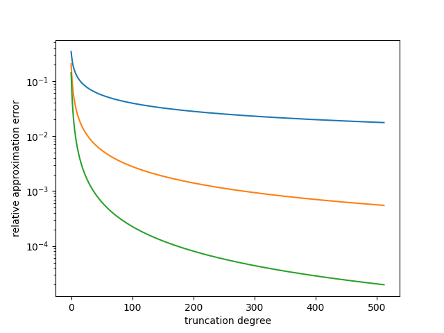
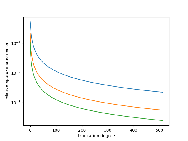
Figure 11: Variation with truncation degree of the relative approximation error $\left\|\hat{\delta}_{x}-\tilde{\hat{\delta}}_{x}\right\|_{H^{s}(\mathbb{S}^{2})}$ for point evaluation of a function. The left hand panel show the relative error for fixed $\lambda=1.0$ for three values of the Sobolev exponent: 1.5 in blue, 2.0 in orange, and 2.5 in green. The right hand panel then fixes $s=2.0$, and plots the relative error for $\lambda$ equal to: 0.5 in blue, 1.0 in orange, and 1.5 in green.

B.4 The Sobolev embedding theorem

Elements of $H^{s}(\mathbb{S}^{2})$ for $s>0$ form a subset of $L^{2}(\mathbb{S}^{2})$, and so their point-values need not be defined. However, the famous Sobolev embedding theorem shows that if the Sobolev exponent is sufficiently large, then elements of $H^{s}(\mathbb{S}^{2})$ do have well-defined point values, and may also be continuously differentiable up to a finite-order. A proof of this result will not be given, but one can be found in Chapter 4 of Taylor (1996) which is valid for any compact manifold. Here it should be noted again that there are several different means by which Sobolev spaces can be defined, but this does not change either the validity nor form of the embedding theorem.

Theorem B.2

The Sobolev space $H^{s}(\mathbb{S}^{2})$ for $s>k+1$ is continuously, densely, and properly embedded into $C^{k}(\mathbb{S}^{2})$.

Assuming that $s>1$, we can now conclude that the Dirac measure $\delta_{x}$ belongs to $H^{s}(\mathbb{S}^{2})^{\prime}$, and so Theorem B.1 implies

$$u(x)=\left({\hat{\delta}_{x}},{u}\right)_{H^{s}(\mathbb{S}^{2})},$$ (222)

for all $u\in H^{s}(\mathbb{S}^{2})$, where the $H^{s}(\mathbb{S}^{2})$-representation of $\delta_{x}$ is given by

$$\hat{\delta}_{x}=\sum_{l\in\mathbb{N}}\left\langle{l}\right\rangle_{\lambda}^{-2s}\sum_{m=-l}^{l}Y_{lm}(x)Y_{lm}.$$ (223)

The Cauchy-Schwarz inequality leads to the sharp bound

$$|u(x)|\leq\|\hat{\delta}_{x}\|_{H^{s}(\mathbb{S}^{2})}\|u\|_{H^{s}(\mathbb{S}^{2})},$$ (224)

where $\|\hat{\delta}_{x}\|_{H^{s}(\mathbb{S}^{2})}$ can be determined using the spherical harmonic addition theorem (e.g. Dahlen & Tromp, 1998, Section B.6)

$$\|\hat{\delta}_{x}\|^{2}_{H^{s}(\mathbb{S}^{2})}=\sum_{l\in\mathbb{N}}\left\langle{l}\right\rangle_{\lambda}^{-2s}\sum_{m=-l}^{l}Y_{lm}(x)Y_{lm}(x)=\sum_{l\in\mathbb{N}}\frac{2l+1}{4\pi}\left\langle{l}\right\rangle_{\lambda}^{-2s}.$$ (225)

Taking the supremum over $x\in\mathbb{S}^{2}$ in eq.(224) we arrive at the the useful estimate

$$\|u\|_{C^{0}(\mathbb{S}^{2})}\leq\left(\sum_{l\in\mathbb{N}}\frac{2l+1}{4\pi}\left\langle{l}\right\rangle_{\lambda}^{-2s}\right)^{\frac{1}{2}}\|u\|_{H^{s}(\mathbb{S}^{2})},$$ (226)

for $u\in H^{s}(\mathbb{S}^{2})$ for $s>1$. In a similar manner is can be shown that when $s>k+1$ we have

$$\|\Delta^{\frac{k}{2}}u\|_{C^{0}(\mathbb{S}^{2})}\leq\left(\sum_{l\in\mathbb{N}}\frac{2l+1}{4\pi}\left\langle{l}\right\rangle_{\lambda}^{-2s}[l(l+1)]^{k}\right)^{\frac{1}{2}}\|u\|_{H^{s}(\mathbb{S}^{2})}.$$ (227)

Here $\Delta^{k/2}$ denotes a fractional power of the Laplace-Beltrami operator, this being defined through its action

$$\Delta^{\frac{k}{2}}u=\sum_{l\in\mathbb{N}}[l(l+1)]^{\frac{k}{2}}\mathbb{P}_{l}u,$$ (228)

for a suitably regular function. The utility of eq.(227) is that the left hand side provides a rotationally invariant, and computationally simple, proxy for the magnitude of a functions $k$th derivatives.

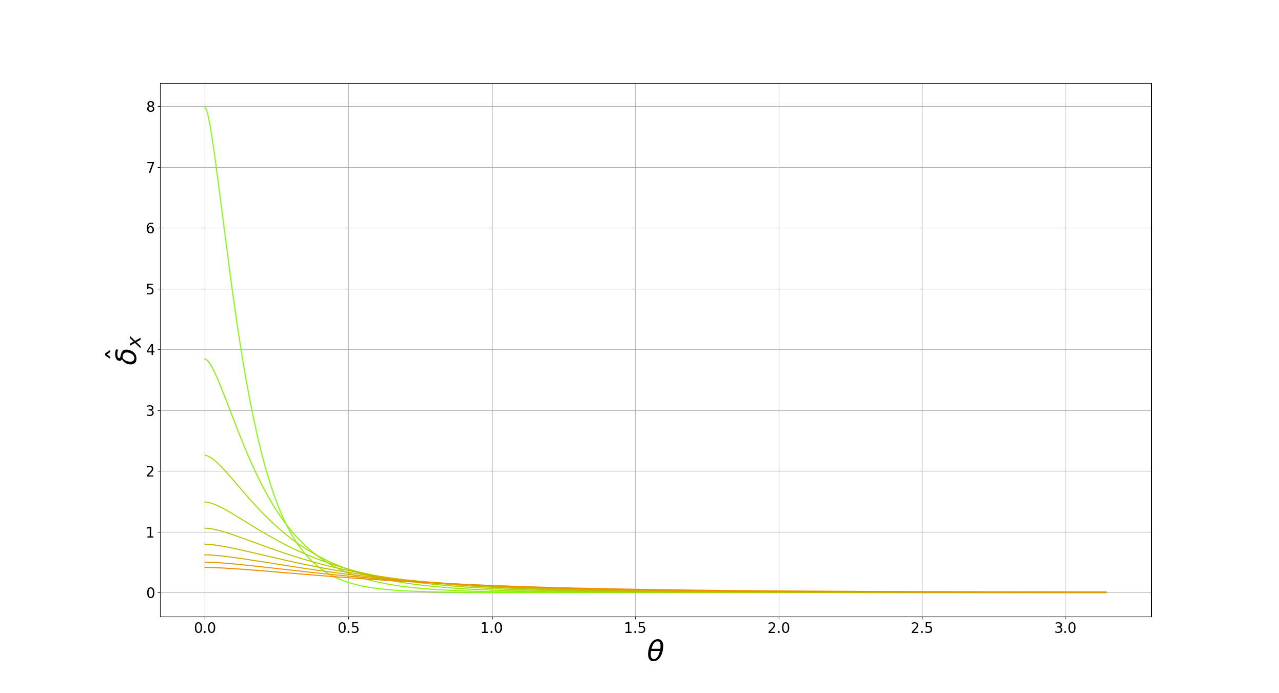
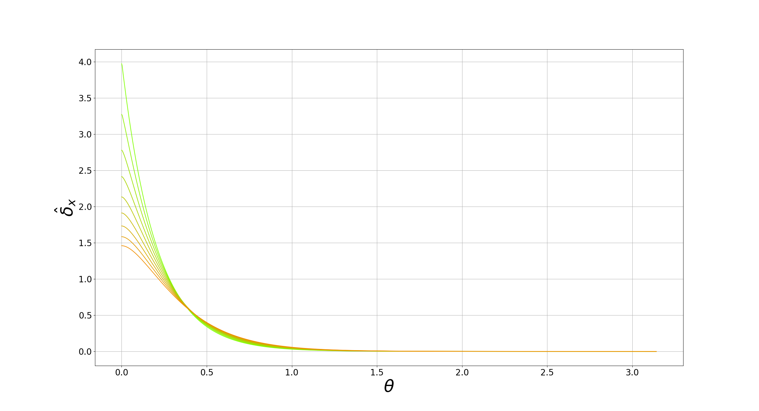
Figure 12: The $H^{s}(\mathbb{S}^{2})$-representation of a Dirac measure $\hat{\delta}_{x}$ as a function of the angle $\theta$ defined within eq.(234). Within the upper plot the value of the Sobolev exponent $s$ is fixed at $2$, while $\lambda$ is spaced equally between $0.1$ (green) and $0.5$ (orange), with the colours grading smoothly between these limits. The lower plot is made in the same manner, but with fixed $\lambda=0.2$ and $s$ ranging from $1.5$ (green) to $2.5$ (orange).

B.5 Numerical implementation

The Sobolev spaces $H^{s}(\mathbb{S}^{2})$ are infinite-dimensional, and so their elements must be suitably approximated within any numerical work. An obvious way to do this is with truncated spherical harmonic expansions up to some maximum degree $L$. Thus, given a function $u\in H^{s}(\mathbb{S}^{2})$, its truncated expansion to degree $L$ is defined by

$$u_{L}=\sum_{l=0}^{L}\mathbb{P}_{l}u.$$ (229)

Consider a linear functional $u^{\prime}\in H^{s}(\mathbb{S}^{2})^{\prime}$, and let $v$ denote its $H^{s}(\mathbb{S}^{2})$-representation such that

$$\left\langle{u^{\prime}},{u}\right\rangle=\left({v},{u}\right)_{H^{s}(\mathbb{S}^{2})},$$ (230)

for all $u\in H^{s}(\mathbb{S}^{2})$. Acting such a functional on $u_{L}$ we obtain

$$\left\langle{u^{\prime}},{u_{L}}\right\rangle=\sum_{l=0}^{L}\left({v},{\mathbb{P}_{l}u}\right)_{H^{s}(\mathbb{S}^{2})}=\sum_{l=0}^{L}\left({\mathbb{P}_{l}v},{u}\right)_{H^{s}(\mathbb{S}^{2})}=\left({v_{L}},{u}\right)_{H^{s}(\mathbb{S}^{2})},$$ (231)

where $v_{L}$ denotes the truncated expansion of $v$. The Cauchy-Schwarz inequality leads to the sharp error-estimate

$$|\left\langle{u^{\prime}},{u}\right\rangle-\left\langle{u^{\prime}},{u_{L}}\right\rangle|\leq\|v-v_{L}\|_{H^{s}(\mathbb{S}^{2})}\|u\|_{H^{s}(\mathbb{S}^{2})}.$$ (232)

It follows that if a prior bound on $\|u\|_{H^{s}(\mathbb{S}^{2})}$ is known, we can choose a truncation degree $L$ such that the absolute error in $\left\langle{u^{\prime}},{u}\right\rangle$ is as small as desired. This method trivially extends to any finite collection of linear functionals, and in this manner we can ensure that the numerical discretisation of a linear inference problem is sufficiently accurate. To illustrate this idea, consider point-evaluation of a function. Here the relevant functional is $\delta_{x}$ for some $x\in\mathbb{S}^{2}$, and we write $\hat{\delta}_{x}$ for its $H^{s}(\mathbb{S}^{2})$-representation whose concrete form is given by eq.(223). Applying the spherical harmonic addition theorem we obtain

$$\left\|\hat{\delta}_{x}-\hat{\delta}_{x,L}\right\|_{H^{s}(\mathbb{S}^{2})}=\left(\sum_{l=L+1}^{\infty}\frac{2l+1}{4\pi}\left\langle{l}\right\rangle_{\lambda}^{-2s}\right)^{\frac{1}{2}},$$ (233)

where $\hat{\delta}_{x,L}$ denotes the truncated expansion of $\hat{\delta}_{x}$. Using this expression, we plot in Fig.11 the variation of the relative approximation error with truncation degree $L$ for a range of values of $s$ and $\lambda$. In practice, however, these worse-case error estimates are overly conservative, with convergence usually being obtained at substantially lower truncation degrees.

Building on this example, we can examine visually the dependence of the $H^{s}(\mathbb{S}^{2})$-representation of the Dirac measure $\delta_{x}$ on the parameters $s>1$ and $\lambda>0$. Again using the spherical harmonic addition theorem, eq.(223) can be simplified to

$$\hat{\delta}_{x}(y)=\sum_{l\in\mathbb{N}}\left\langle{l}\right\rangle_{\lambda}^{-2s}\frac{2l+1}{4\pi}P_{l}(\cos\theta),$$ (234)

where $P_{l}$ is a Legendre polynomial of degree $l$, and $\theta$ is the angle between $x,y\in\mathbb{S}^{2}$. Plots of this function are shown in Fig.12 for a range of values of $s$ and $\lambda$. Within these calculations the truncation degree $L$ was chosen so that the relative approximation error always lies below $10^{-5}$ which is sufficient for visual inspection. As a general trend, it is seen that as either $s>1$ or $\lambda>0$ decreases, the function becomes more sharply peaked at $\theta=0$. Nonetheless, in each case the Dirac measure is, in accordance with the Sobolev embedding theorem, represented by a continuous function that can be accurately captured by truncated spherical harmonic expansions.

References

- Backus (1970a) Backus, G. E., 1970a. Inference from inadequate and inaccurate data, i, Proceedings of the National Academy of Sciences, 65(1), 1–7.
- Backus (1970b) Backus, G. E., 1970b. Inference from inadequate and inaccurate data, i, Proceedings of the National Academy of Sciences, 65(1), 281–287.
- Backus (1970c) Backus, G. E., 1970c. Inference from inadequate and inaccurate data, iii, Proceedings of the National Academy of Sciences, 67(1), 282–289.
- Backus (1972) Backus, G. E., 1972. Inference from inadequate and inaccurate data, in Mathematical Problems in the Geophysical Sciences, chap. 1, pp. 1–105, ed. Reid, W., American Mathematical Society, Providence, Rhode Island.
- Backus (1988) Backus, G. E., 1988. Bayesian inference in geomagnetism, Geophysical Journal International, 92(1), 125–142.
- Backus (1989) Backus, G. E., 1989. Confidence set inference with a prior quadratic bound, Geophysical Journal International, 97(1), 119–150.
- Backus (1996) Backus, G. E., 1996. Trimming and procrastination as inversion techniques, Physics of the earth and planetary interiors, 98(3-4), 101–142.
- Backus & Gilbert (1967) Backus, G. E. & Gilbert, F., 1967. Numerical applications of a formalism for geophysical inverse problems, Geophys. J. R. Astron. Soc., 13(1-3), 247–276.
- Backus & Gilbert (1968) Backus, G. E. & Gilbert, F., 1968. The resolving power of gross Earth data, Geophys. J. R. Astron. Soc., 16(2), 169–205.
- Backus & Gilbert (1970) Backus, G. E. & Gilbert, F., 1970. Uniqueness in the inversion of inaccurate gross earth data, Phil. Trans. R. Soc. Lond. A, 266(1173), 123–192.
- Blazek et al. (2013) Blazek, K. D., Stolk, C., & Symes, W. W., 2013. A mathematical framework for inverse wave problems in heterogeneous media, Inverse Problems, 29(6), 065001.
- Bogachev (1996) Bogachev, V., 1996. Gaussian measures on linear spaces, Journal of Mathematical Sciences, 79(2), 933–1034.
- Bump (2004) Bump, D., 2004. Lie groups, Springer, Berlin.
- Constable et al. (1987) Constable, S. C., Parker, R. L., & Constable, C. G., 1987. Occam’s inversion: A practical algorithm for generating smooth models from electromagnetic sounding data, Geophysics, 52(3), 289–300.
- Crawford et al. (2018) Crawford, O., Al-Attar, D., Tromp, J., Mitrovica, J. X., Austermann, J., & Lau, H. C., 2018. Quantifying the sensitivity of post-glacial sea level change to laterally varying viscosity, Geophysical journal international, 214(2), 1324–1363.
- Dahlen & Tromp (1998) Dahlen, F. A. & Tromp, J., 1998. Theoretical Global Seismology, Princeton University Press.
- Evans & Stark (2002) Evans, S. N. & Stark, P. B., 2002. Inverse problems as statistics, Inverse problems, 18(4), R55.
- Freeden & Hermann (1986) Freeden, W. & Hermann, P., 1986. Uniform approximation by spherical spline interpolation, Mathematische Zeitschrift, 193(2), 265–275.
- Genovese & Stark (1996) Genovese, C. R. & Stark, P. B., 1996. Data reduction and statistical inconsistency in linear inverse problems, Physics of the earth and planetary interiors, 98(3-4), 143–162.
- Gubbins (2004) Gubbins, D., 2004. Time series analysis and inverse theory for geophysicists, Cambridge University Press.
- Hoggard et al. (2016) Hoggard, M. J., White, N., & Al-Attar, D., 2016. Global dynamic topography observations reveal limited influence of large-scale mantle flow, Nature Geoscience, 9(6), 456.
- Ishii & Tromp (1999) Ishii, M. & Tromp, J., 1999. Normal-mode and free-air gravity constraints on lateral variations in velocity and density of earth9s mantle, Science, 285(5431), 1231–1236.
- James (1964) James, R. C., 1964. Weakly compact sets, Transactions of the American Mathematical Society, 113(1), 129–140.
- Kammerer & Nashed (1972) Kammerer, W. J. & Nashed, M. Z., 1972. On the convergence of the conjugate gradient method for singular linear operator equations, SIAM Journal on Numerical Analysis, 9(1), 165–181.
- Kelley (1955) Kelley, J. L., 1955. General topology, Van Nostrand, New York.
- Kuo (1975) Kuo, H.-H., 1975. Gaussian Measures in Banach Spaces, Springer, Berlin.
- Lang (2012) Lang, S., 2012. Fundamentals of differential geometry, vol. 191, Springer, Berlin.
- Lau et al. (2017) Lau, H. C., Mitrovica, J. X., Davis, J. L., Tromp, J., Yang, H.-Y., & Al-Attar, D., 2017. Tidal tomography constrains earth’s deep-mantle buoyancy, Nature, 551(7680), 321.
- Li et al. (2011) Li, K., Jackson, A., & Livermore, P. W., 2011. Variational data assimilation for the initial-value dynamo problem, Phys. Rev. E., 84(5), 056321.
- Lions & Magenes (1972) Lions, J. L. & Magenes, E., 1972. Non-homogeneous boundary value problems and applications: Vol. 1, vol. 181, Springer, Berlin.
- Luenberger (1997) Luenberger, D. G., 1997. Optimization by vector space methods, John Wiley & Sons.
- Mayo (2018) Mayo, D. G., 2018. Statistical inference as severe testing, Cambridge: Cambridge University Press.
- Menke (2018) Menke, W., 2018. Geophysical data analysis: Discrete inverse theory, Academic press.
- Moré & Thuente (1994) Moré, J. J. & Thuente, D. J., 1994. Line search algorithms with guaranteed sufficient decrease, ACM Transactions on Mathematical Software (TOMS), 20(3), 286–307.
- Nocedal & Wright (2006) Nocedal, J. & Wright, S., 2006. Numerical optimization, Springer, Berlin.
- Øksendal (2003) Øksendal, B., 2003. Stochastic differential equations, in Stochastic differential equations, pp. 65–84, Springer.
- Parker (1972) Parker, R. L., 1972. Inverse theory with grossly inadequate data, Geophysical Journal International, 29(2), 123–138.
- Parker (1977) Parker, R. L., 1977. Linear inference and underparameterized models, Reviews of Geophysics, 15(4), 446–456.
- Parker (1994) Parker, R. L., 1994. Geophysics Inverse Theory, Princeton University Press.
- Pijpers & Thompson (1992) Pijpers, F. P. & Thompson, M. J., 1992. Faster formulations of the optimally localized averages method for helioseismic inversions, Astronomy and Astrophysics, 262, L33–L36.
- Pijpers & Thompson (1994) Pijpers, F. P. & Thompson, M. J., 1994. The SOLA method for helioseismic inversion, Astronomy and Astrophysics, 281, 231–240.
- Sambridge et al. (2006) Sambridge, M., Gallagher, K., Jackson, A., & Rickwood, P., 2006. Trans-dimensional inverse problems, model comparison and the evidence, Geophysical Journal International, 167(2), 528–542.
- Shubin (1987) Shubin, M. A., 1987. Pseudodifferential operators and spectral theory, vol. 200, Springer, Berlin.
- Spivak (1970) Spivak, M. D., 1970. A comprehensive introduction to differential geometry, Publish or perish.
- Stark (2008) Stark, P. B., 2008. Generalizing resolution, Inverse Problems, 24(3), 034014.
- Stark (2015) Stark, P. B., 2015. Constraints versus priors, SIAM/ASA Journal on Uncertainty Quantification, 3(1), 586–598.
- Stuart (2010) Stuart, A. M., 2010. Inverse problems: a bayesian perspective, Acta numerica, 19, 451–559.
- Tape et al. (2007) Tape, C., Liu, Q., & Tromp, J., 2007. Finite-frequency tomography using adjoint methods - Methodology and examples using membrane surface waves, Geophys. J. Int., 168(3), 1105–1129.
- Tarantola (2005) Tarantola, A., 2005. Inverse problem theory and methods for model parameter estimation, vol. 89, siam.
- Taylor (1996) Taylor, M. E., 1996. Partial differential equations. 1, Basic theory, Springer, Berlin.
- Treves (1967) Treves, F., 1967. Topological Vector Spaces, Distributions and Kernels, Academic Press, New York.
- Vakhania et al. (1987) Vakhania, N., Tarieladze, V., & Chobanyan, S., 1987. Probability distributions on Banach spaces, vol. 14, Springer, Berlin.
- Valentine & Davies (2020) Valentine, A. P. & Davies, D. R., 2020. Global models from sparse data: A robust estimate of earth’s residual topography spectrum, Geochemistry, Geophysics, Geosystems, 21(8), e2020GC009240.
- Valentine & Sambridge (2020a) Valentine, A. P. & Sambridge, M., 2020a. Gaussian process models—i. a framework for probabilistic continuous inverse theory, Geophysical Journal International, 220(3), 1632–1647.
- Valentine & Sambridge (2020b) Valentine, A. P. & Sambridge, M., 2020b. Gaussian process models—ii. lessons for discrete inversion, Geophysical Journal International, 220(3), 1648–1656.
- Wiggins (1972) Wiggins, R. A., 1972. The general linear inverse problem: Implication of surface waves and free oscillations for earth structure, Reviews of Geophysics, 10(1), 251–285.
- Wunsch (2006) Wunsch, C., 2006. Discrete inverse and state estimation problems: with geophysical fluid applications, Cambridge University Press.
- Zaroli (2016) Zaroli, C., 2016. Global seismic tomography using backus–gilbert inversion, Geophysical Supplements to the Monthly Notices of the Royal Astronomical Society, 207(2), 876–888.
- Zaroli (2019) Zaroli, C., 2019. Seismic tomography using parameter-free backus–gilbert inversion, Geophysical Journal International, 218(1), 619–630.
- Zuberi & Pratt (2017) Zuberi, M. A. & Pratt, R., 2017. Mitigating nonlinearity in full waveform inversion using scaled-sobolev pre-conditioning, Geophysical Journal International, 213(1), 706–725.