Mapping Dirac–Hartree–Fock approach onto relativistic mean field model

Abstract

The exchange part of energy density of the linear Dirac–Hartree–Fock (DHF) model in symmetric nuclear matter is evaluated in a parameter–free closed form and expressed as density functional. After the rearranging terms the relativistic mean-field approach with density-dependent couplings may be recovered with density dependence coming from the Fock exchange. The formalism developed, is then extended to the nonlinear DHF approximation with field self-couplings allowed. The nonlinear self–interactions result in essential density dependence (medium modification) of effective couplings that are decoupled from the Fock ones.

I Introduction

Kohn and Sham’s density functional theory (DFT) [1, *Kohn:1965] has developed into one of the most successful approaches ever for a description of the electronic structure of matter. It provides the great variety of ground–state properties of a system with the electron density playing the key role.

Inspired by the achievements of the coulombic DFT, there is an ambition of current nuclear physics to develop the (energy) density functional for a proper description of exotic nuclei and equation–of–state (EOS) of nuclear matter (see e.g. [3, *Schmid:1995a] for early approaches and [5, *Meng:2016, *Lalazissis:2004] for recent reviews). A suitable starting candidate seems to be the relativistic mean–field (RMF) theory [8, 9]. The RMF model has greatly contributed to our understanding of nuclear structure, and it was intensively used over years for a description of a wide class of nuclear phenomena (see e.g. [10] and references therein for reviews). Two mutually independent versions of the RMF approach have been developed, either one with nonlinear self–interactions of meson fields [11, 12, 13, 14], or one with density–dependent meson–nucleon couplings [15, 16, 17, 18]. Both approaches cast the additional density dependence into the effective interaction that is inevitable for a proper description of nuclear systems.

The density–dependent couplings in the relativistic mean–field approaches are introduced phenomenologically. They are often determined by comparison with Dirac–Brueckner–Hartree–Fock (DBHF) calculations for nuclear matter [19, 20, 21, 22, 23] in limited range of densities. Their functional forms are usually chosen ad–hoc; the choice being dictated mainly by the requirement of simplicity. Most authors employ the rational form. Various functions of density dependences used are discussed in Ref. [24] together with their extrapolation properties out of fitted interval of densities. Especially, the couplings for low–density region (relevant for a nuclear periphery of exotic nuclei) and high–density one (typical for neutron star calculations) are not reliably determined by extrapolations.

Also, there exist approaches incorporating the exchange (Fock) terms into the relativistic description of nuclear matter and finite nuclei. The relativistic Dirac–Hartree–Fock (DHF) approach [25, 26] has been developed together with its own density–dependent versions [27, 28]. The exchange parts give rise to the state–dependent potentials due to nonlocal character of the DHF approach and the solutions of Dirac equations for finite nuclei thus require much more numerically intensive efforts than in the RMF model.

To simplify the problem, the concept of equivalent local potentials to the nonlocal exchange ones was intensively developed from early applications of the DHF mean–field approach [8, 29]. Next step was done in Refs. [4, 30] where the exchange energy density of the $\sigma$–$\omega$ model was evaluated analytically in nuclear matter using the dilogarithm integrals, and its density dependence was used to construct a local effective exchange potential. Greco et al. [31] treated the Fock exchange term in a “kinetic approach” employing the Wigner transform formalism. The approach was restricted to the $\sigma$–$\omega$ model with the scalar self–interaction terms.

It is, therefore, of interest to develop an approach as simple as the RMF model that will account for exchange correlations, at least for nuclear matter [32].

The present paper is aimed at mapping the Fock exchange terms of the DHF energy density for nuclear matter onto its Hartree parts. An explicit evaluation of the exchange integrals leads to the RMF theory with density–dependent couplings. The analytical functional density dependence of couplings obtained thus accounts for exchange correlations over a full range of densities. This may significantly reduce the arbitrariness of couplings at low and high densities.

For simplicity, we will treat the symmetric nuclear matter case and consider the exchange of isoscalar mesons only, together with $\pi$–meson. While the former gives the dominant contributions in both, the RMF and DHF approaches, the pionic field contributes only in an exchange part of the DHF model. This illustrates the essential points of the approach. The generalization for asymmetric nuclear matter and the full set of exchanged mesons can be made straightforwardly.

II DHF energy density for symmetric nuclear matter

We start with the effective Lagrangian density for the interacting nucleons ($\psi$) and the scalar $\sigma$, vector $\omega$, and pion $\pi$ fields,

$${\mathcal{L}}={\mathcal{L}}_{0}+{\mathcal{L}}_{I}\;,$$ (1)

consisting of the free part

$${\mathcal{L}}_{0} = \overline{\psi}(i\gamma_{\mu}\partial^{\mu}-M)\psi+\frac{1}{2}(\partial_{\mu}\sigma\partial^{\mu}\sigma-m_{\sigma}^{2}\sigma^{2})$$

$$-\frac{1}{4}\omega_{\mu\nu}\omega^{\mu\nu}+\frac{1}{2}m_{\omega}^{2}\omega_{\mu}\omega^{\mu}+\frac{1}{2}(\partial_{\mu}\pi\partial^{\mu}\pi-m_{\pi}^{2}\pi^{2})\;,$$

where $\omega_{\mu\nu}=\partial_{\mu}\omega_{\nu}-\partial_{\nu}\omega_{\mu}$, and the interaction term

$${\mathcal{L}}_{I}=-g_{\sigma}\overline{\psi}\sigma\psi-g_{\omega}\overline{\psi}\gamma_{\mu}\omega^{\mu}\psi-\frac{f_{\pi}}{m_{\pi}}\overline{\psi}\gamma_{5}\gamma_{\mu}(\partial^{\mu}\pi)\psi\;.$$ (3)

Here, the symbol $M$ denotes the nucleon rest mass, whereas $g_{i}$ ($f_{i}$), $m_{i}$, $i=\{\sigma,\omega,\pi\}$ mean the coupling constants and rest masses for the scalar ($\sigma$), vector ($\omega$) and pseudoscalar ($\pi$) mesons, respectively. The direct Yukawa couplings are used for the $\sigma$ and $\omega$ fields, while the pseudovector coupling is applied for the pion.

To keep the paper self–explanatory we repeat here some basic facts of the Dirac–Hartree–Fock approach for nuclear matter. They are based mostly on Refs. [33] and [34].

Due to parity and time–reversal symmetry, the nuclear matter self–energy $\Sigma$ takes a form

$$\Sigma(k)=\Sigma^{s}(k)+\gamma^{0}\Sigma^{0}(k)+\bm{\gamma}\cdot\bm{k}\Sigma^{v}(k)\;,$$ (4)

where superscripts $\{s,0,v\}$ denote the scalar, time–like and space–like components of the self–energy, consecutively.

Dirac equation for nuclear matter is then written as

$$(\bm{\alpha}\cdot\bm{k^{\star}}+\beta M^{\star})u(\bm{k},s)=E^{\star}u(\bm{k},s),$$ (5)

with the positive energy solution being

$$u(\bm{k},s)=\left(\frac{E^{\star}+M^{\star}}{2E^{\star}}\right)^{1/2}\left(\begin{array}[]{c}1\\ \dfrac{\bm{\sigma}\cdot\bm{k^{\star}}}{E^{\star}+M^{\star}}\end{array}\right)\chi_{s}\;.$$ (6)

Here $\chi_{s}$ is a two–component Pauli spinor, and the starred quantities are defined via the self–energy components as

$$\bm{k^{\star}}=\bm{k}+\bm{k}\Sigma^{v}(k),$$ (7a)

$$M^{\star}=M+\Sigma^{s}(k),$$ (7b)

$$E^{\star}=E-\Sigma^{0}(k),$$ (7c)

and the on–shell condition is

$${E^{\star}}^{2}=({M^{\star}}^{2}+{\bm{k^{\star}}}^{2})\;.$$ (8)

Additionally, the auxiliary functions $\hat{P}$ and $\hat{M}$ are introduced by relations

$$\hat{P}(k)=k^{\star}/E^{\star},$$ (9a)

$$\hat{M}(k)=M^{\star}/E^{\star}.$$ (9b)

The energy functional, i.e., the nuclear matter energy density, is given as (00)–component of the momentum–energy tensor. Alternatively, it is obtained by taking the expectation value of the Hamiltonian $\mathcal{H}$ with respect to the ground state $\left|\Psi_{0}\right>$ in a given volume $\Omega$,

$$\mathcal{E}=\frac{1}{\Omega}\left<\Psi_{0}\right|\mathcal{H}\left|\Psi_{0}\right>\equiv\left<\mathcal{T}\right>+\left<\mathcal{V}\right>,$$ (10)

and expressed as the sum of kinetic $\mathcal{T}$ and potential energy $\mathcal{V}$ parts.

The potential energy density $\left<\mathcal{V}\right>$ of the DHF approach can be decomposed into the direct (Hartree) term, $\varepsilon^{D}$, and the exchange (Fock) contribution, $\varepsilon^{X}$,

$$\left<\mathcal{V}\right>=\varepsilon^{D}+\varepsilon^{X}\;.$$ (11)

The direct energy density reads

$$\varepsilon^{D}=-\frac{1}{2}\frac{g_{\sigma}^{2}}{m_{\sigma}^{2}}\rho_{S}^{2}+\frac{1}{2}\frac{g_{\omega}^{2}}{m_{\omega}^{2}}\rho_{B}^{2}\;,$$ (12)

where the scalar density $\rho_{S}$ and the vector (baryon) one $\rho_{B}$ were used. They are the sources of the corresponding meson–fields at the Hartree (mean–field) level and are simply expressed via the nucleon Fermi momentum $k_{F}$ in the nuclear matter as,

$$\rho_{B}(k_{F}) = \frac{4}{(2\pi)^{3}}\int_{0}^{k_{F}}d^{3}q=\frac{4}{6\pi^{2}}k_{F}^{3}\;,$$ (13)

$$\rho_{S}(k_{F},M^{\star}) = \frac{4}{(2\pi)^{3}}\int_{0}^{k_{F}}d^{3}q\frac{M^{\star}(q)}{E^{\star}(q)}\;.$$ (14)

The pre–integral numerical factors of 4 reflect the spin/isospin degeneracy of the nucleons in symmetric nuclear matter. Only the $\sigma$ and $\omega$ mesons with direct couplings contribute to $\varepsilon^{D}$. As it is already expressed in terms of densities, it has the proper form for use in the DFT approach.

Variation of $\varepsilon^{D}$ with respect to the Dirac spinor gives the direct contributions to the scalar, $\Sigma^{s}$, and time–like vector, $\Sigma^{0}$, components of the self–energy. One obtains,

$$\Sigma^{s}=-\dfrac{g_{\sigma}^{2}}{m_{\sigma}^{2}}\rho_{S},\qquad\Sigma^{0}=\dfrac{g_{\omega}^{2}}{m_{\omega}^{2}}\rho_{B}\;.$$ (15)

There is no contribution to space–like part of the vector component of the self–energy.

In contrast to the direct (Hartree) energy density the exchange (Fock) energy density, $\varepsilon^{X}$, has a more complicated structure. All mesons contribute to the exchange energy density and it does not exhibit the explicit dependence on nuclear densities:

$$\varepsilon^{X}=\sum\limits_{\kappa}\varepsilon_{\kappa}^{X},\hskip 30.00005pt\kappa=\{\sigma,\omega,\pi\}$$ (16)

$$\varepsilon_{\kappa}^{X} = \frac{1}{(2\pi)^{4}}\int\limits_{0}^{k_{F}}k\,dk\int\limits_{0}^{k_{F}}q\,dq\left[A_{\kappa}(k,q)\right.$$

$$\left.+\hat{M}(k)\hat{M}(q)B_{\kappa}(k,q)+\hat{P}(k)\hat{P}(q)C_{\kappa}(k,q)\right]\;,$$

where $A_{\kappa}$, $B_{\kappa}$, $C_{\kappa}$ are known functions for each meson exchanged and interaction type considered (e.g. Ref. [26]); they are listed in Table 1 for mesons involved in the present paper. The terms contain the angular exchange integrals $\Theta_{\kappa}$ and $\Phi_{\kappa}$ for $\kappa=\{\sigma,\omega,\pi\}$ given as

$$\Theta_{\kappa}(k,q)=\ln\frac{(k+q)^{2}+m_{\kappa}^{2}}{(k-q)^{2}+m_{\kappa}^{2}}\;,$$ (18)

and

$$\Phi_{\kappa}(k,q)=\frac{1}{4kq}(k^{2}+q^{2}+m_{\kappa}^{2})\Theta_{\kappa}(k,q)-1\;,$$ (19)

where we already omitted the retardation effects in the meson propagators.

Table 1: The terms $A_{\kappa}$, $B_{\kappa}$, and $C_{\kappa}$ of Eq. (II)

$\kappa$	$A_{\kappa}(k,q)$	$B_{\kappa}(k,q)$	$C_{\kappa}(k,q)$
$\sigma$	$g_{\sigma}^{2}\Theta_{\sigma}$	$g_{\sigma}^{2}\Theta_{\sigma}$	$-2g_{\sigma}^{2}\Phi_{\sigma}$
$\omega$	$2g_{\omega}^{2}\Theta_{\omega}$	$-4g_{\omega}^{2}\Theta_{\omega}$	$-4g_{\omega}^{2}\Phi_{\omega}$
$\pi$	$-3\left(\dfrac{f_{\pi}}{m_{\pi}}\right)^{2}m_{\pi}^{2}\Theta_{\pi}$	$-3\left(\dfrac{f_{\pi}}{m_{\pi}}\right)^{2}m_{\pi}^{2}\Theta_{\pi}$	$C_{\pi}$
	$C_{\pi}=6\left(\dfrac{f_{\pi}}{m_{\pi}}\right)^{2}\left[\left(k^{2}+q^{2}\right)\Phi_{\pi}-kq\Theta_{\pi}\right]$

Nevertheless, using the approach developed in Appendix A, we were able to evaluate all the exchange integrals in Eq. (II). Then with the results reached one may write down all contributions to the exchange energy density in the closed–form.

Namely, for the $\sigma$–meson exchange we obtain

$$\varepsilon_{\sigma}^{X} = \frac{1}{16}\frac{g^{2}_{\sigma}}{m^{2}_{\sigma}}X_{\theta}(k_{F}/m_{\sigma})\rho_{B}^{2}(k_{F})$$

$$+ \frac{1}{16}\frac{g^{2}_{\sigma}}{m^{2}_{\sigma}}X_{\theta}(k_{F}/m_{\sigma})\rho_{S}^{2}(k_{F},M^{\star})$$

$$- \frac{2}{16}\frac{g^{2}_{\sigma}}{m^{2}_{\sigma}}X_{\phi}(k_{F}/m_{\sigma})\left(\rho_{B}^{2}(k_{F})-\rho_{S}^{2}(k_{F},M^{\star})\right)\;.$$

The first line on the right-hand-side (rhs) of the last equation comes from the evaluation of A–function term of Eq. (II). It depends on the square of vector (baryon) density $\rho_{B}$. Additional density dependence is due to the exchange shape function $X_{\theta}$ via the dimensionless Fermi momentum variable $x=k_{F}/m_{\sigma}$. After variation it contributes to the time–like vector component of the self–energy.

The term on the second line of the rhs is from the evaluation of B–function integral. It depends on the square of the scalar density. Similarly, as in the previous case, the additional density dependence is determined by the function $X_{\theta}(k_{F}/m_{\sigma})$. It gives contribution to the scalar component of the self–energy.

The last term on the third line has a different structure. It comes from the integration of the C–function term. Firstly, the additional density dependence is due to the function $X_{\phi}$. It behaves differently in comparison with the function $X_{\theta}$. It vanishes at zero density and grows very slowly with increasing Fermi momentum. The comparison of both, the $X_{\theta}$ and $X_{\phi}$ exchange shape functions, is shown in Fig. 1. (Note that $X_{\phi}$ is scaled by a factor of 10 for better clarity.) Secondly, the term depends on the difference of squares of the baryon and scalar densities, respectively. Thus the term that in the DHF approach contributes to the space–like vector component of the self–energy is split up to the scalar and time–like vector components of the self–energy in the current procedure. The DHF space–like component is thus being effectively eliminated.

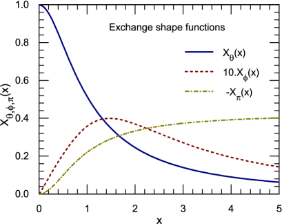
Figure 1: (Color online.) The graph of the exchange shape functions $X_{\theta}(x)$, $X_{\phi}(x)$, and $X_{\pi}(x)$. The $X_{\phi}$ function is scaled by a factor of 10 for clarity, and the sign of the function $X_{\pi}$ was changed to the opposite one to keep the figure compact.

For the $\omega$–meson exchange one writes

$$\varepsilon_{\omega}^{X} = \frac{2}{16}\frac{g^{2}_{\omega}}{m^{2}_{\omega}}X_{\theta}(k_{F}/m_{\omega})\rho_{B}^{2}(k_{F})$$

$$- \frac{4}{16}\frac{g^{2}_{\omega}}{m^{2}_{\omega}}X_{\theta}(k_{F}/m_{\omega})\rho_{S}^{2}(k_{F},M^{\star})$$

$$- \frac{4}{16}\frac{g^{2}_{\omega}}{m^{2}_{\omega}}X_{\phi}(k_{F}/m_{\omega})\left(\rho_{B}^{2}(k_{F})-\rho_{S}^{2}(k_{F},M^{\star})\right)\;,$$

and the $\pi$–meson exchange contribution is

$$\varepsilon_{\pi}^{X} = -\frac{3}{16}\left(\dfrac{f_{\pi}}{m_{\pi}}\right)^{2}X_{\theta}(k_{F}/m_{\pi})\rho_{B}^{2}(k_{F})$$

$$- \frac{3}{16}\left(\dfrac{f_{\pi}}{m_{\pi}}\right)^{2}X_{\theta}(k_{F}/m_{\pi})\rho_{S}^{2}(k_{F},M^{\star})$$

$$+ \frac{6}{16}\left(\dfrac{f_{\pi}}{m_{\pi}}\right)^{2}X_{\pi}(k_{F}/m_{\pi})\left(\rho_{B}^{2}(k_{F})-\rho_{S}^{2}(k_{F},M^{\star})\right)\;.$$

Similar comments as were made to the $\varepsilon_{\sigma}^{X}$ part, may be applied to the $\varepsilon_{\omega}^{X}$ and $\varepsilon_{\pi}^{X}$ contributions, except the $X_{\pi}$ shape function. It comes from the $C_{\pi}$–term integration (see Appendix A) and its graph is plotted in Fig. 1. Due to smaller rest mass of the pion, the dimensionless variable $x=k_{F}/m_{\pi}$ covers a wider range of values than for other mesons, and thus produces a more pronounced density dependence.

Now, combining the direct and exchange contributions and regrouping them according to the scalar and vector densities, one may write the potential energy density as

$$\left<\mathcal{V}\right>=-\frac{1}{2}\frac{\Gamma_{\sigma}^{2}(k_{F})}{m_{\sigma}^{2}}\rho_{S}^{2}+\frac{1}{2}\frac{\Gamma_{\omega}^{2}(k_{F})}{m_{\omega}^{2}}\rho_{B}^{2}\;,$$ (23)

which resembles the form of the mean–field (Hartree) contribution now, however, with the effective density–dependent couplings $\Gamma_{\sigma}$ and $\Gamma_{\omega}$. They are given by relations

$$\frac{\Gamma_{\sigma}^{2}(k_{F})}{m_{\sigma}^{2}}=\frac{g_{\sigma}^{2}}{m_{\sigma}^{2}} -\frac{1}{8}\frac{g_{\sigma}^{2}}{m_{\sigma}^{2}}X_{\theta}(k_{F}/m_{\sigma})+\frac{4}{8}\frac{g_{\omega}^{2}}{m_{\omega}^{2}}X_{\theta}(k_{F}/m_{\omega})+\frac{3}{8}\left(\frac{f_{\pi}}{m_{\pi}}\right)^{2}X_{\theta}(k_{F}/m_{\pi})$$

$$-\frac{2}{8}\frac{g_{\sigma}^{2}}{m_{\sigma}^{2}}X_{\phi}(k_{F}/m_{\sigma})-\frac{4}{8}\frac{g_{\omega}^{2}}{m_{\omega}^{2}}X_{\phi}(k_{F}/m_{\omega})+\frac{6}{8}\left(\frac{f_{\pi}}{m_{\pi}}\right)^{2}X_{\pi}(k_{F}/m_{\pi})\;,$$

and

$$\frac{\Gamma_{\omega}^{2}(k_{F})}{m_{\omega}^{2}}=\frac{g_{\omega}^{2}}{m_{\omega}^{2}} +\frac{1}{8}\frac{g_{\sigma}^{2}}{m_{\sigma}^{2}}X_{\theta}(k_{F}/m_{\sigma})+\frac{2}{8}\frac{g_{\omega}^{2}}{m_{\omega}^{2}}X_{\theta}(k_{F}/m_{\omega})-\frac{3}{8}\left(\frac{f_{\pi}}{m_{\pi}}\right)^{2}X_{\theta}(k_{F}/m_{\pi})$$

$$-\frac{2}{8}\frac{g_{\sigma}^{2}}{m_{\sigma}^{2}}X_{\phi}(k_{F}/m_{\sigma})-\frac{4}{8}\frac{g_{\omega}^{2}}{m_{\omega}^{2}}X_{\phi}(k_{F}/m_{\omega})+\frac{6}{8}\left(\frac{f_{\pi}}{m_{\pi}}\right)^{2}X_{\pi}(k_{F}/m_{\pi})\;,$$

These relations are the main results of the section. They represent the mean field model with the density–dependent couplings that accounts for exchange correlations from the DHF model in nuclear matter. The approach is parameter–free in the sense that no new parameter was introduced except the DHF ones already used. Actually, in this way we have mapped the DHF model onto the RMF one.

The approach was tested against the results of DHF calculations [26]. Here, we have taken the DHF parameters of row (c) of Table I there, i.e. the parameterization of $\sigma$–$\omega$–$\pi$ DHF model. The comparisons of the exchange contributions to the effective RMF couplings relative to the direct (Hartree) parts for both, the scalar and vector channels, are shown in Fig. 2.

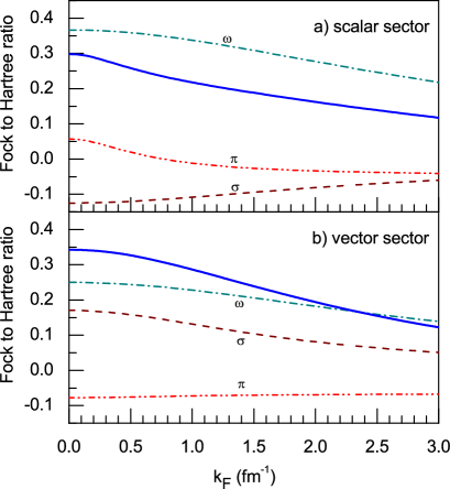
Figure 2: (Color online.) The ratios of Fock (exchange) to Hartree (direct) parts of scalar (upper panel, Eq.(17)) and vector (lower panel, Eq.(15)) vertices, respectively. The thick full line represents the result according to the Eq.(17), resp. Eq.(15), while dashed, dot-dashed and dot-dot-dashed lines are contributions from the exchange of particular mesons. The thin solid curve is a result of a full numerical evaluation of exchange integrals; it practically coincides with the analytical result (thick solid line).

In both channels, the exchange correlations account for $\sim$30% of total coupling strength. This explains the relations already observed in comparisons of the RMF and DHF calculations; the results are similar provided the RMF couplings are suitably renormalized.

The largest exchange contributions to both, the scalar and vector sectors, come from the $\omega$–meson exchange. It contributes from $\sim$25% of the total coupling strength square for the vector sector up to more than $\sim$35% for the scalar channel at zero density and gradually decreases with increasing Fermi momentum $k_{F}$. The scalar meson exchange additions to the total coupling strengths are significantly weaker than the $\omega$–meson ones for both, the scalar and vector channels, respectively. It starts at $\sim-12$% at zero density for the scalar channel and slowly goes to zero for high–density matter. At the vector sector, the scalar contribution starts at $\sim$18% at zero density and again slowly decreases with an increasing one. The $\pi$–meson exchange contributions have a slightly different characters. While the $\sigma$– and $\omega$–exchanges are dominated by the A–term and B–term integrals (due to the $X_{\theta}$ function behavior), leaving the C–term less important (compare the $X_{\phi}$ function vs $X_{\theta}$ one), the $\pi$ contribution depends on the combination of $X_{\theta}$ and $X_{\pi}$ functions. These contribute differently to the scalar and vector sectors, and due to small $\pi$–meson mass, $m_{\pi}$, are of comparable strengths. As a result, the $\pi$–meson addition to the effective scalar coupling square starts at $\sim$6% for zero density, decreases rapidly to $\sim$-5% at saturation and then remains roughly constant up to the dense matter region.

The final sensitive test of the couplings obtained is made by comparison of the original Bouyssy’s results for the binding energy of nuclear matter to our mean–field calculations with Fermi momentum dependent vertices given by Eqs. (II,II). This comparison is shown in Fig. 3. The points are the results of the original DHF calculations [26]. The solid line represents our mean–field calculations with Fermi momentum dependent effective couplings including the direct and all exchange contributions. It compares to the original results fairly well. The dashed line is the mean–field result similar to the solid line, but omitting the contributions containing the $X_{\phi}$ and $X_{\pi}$ exchange shape functions, i.e. omitting the contributions from the space–like mapping on the mean–field approach.

The good agreement is further confirmed with a term–by–term comparison of components of potential energies per nucleon at saturation of both, the DHF calculation [26] and our RMF model with the effective density–dependent couplings. This is done in Table 2.

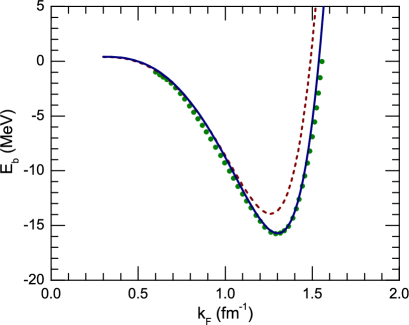
Figure 3: (Color online.) Binding energy per particle in symmetric nuclear matter. The symbols correspond to the DHF results of Ref. [26], and the solid line is the full RMF calculation with $k_{F}$–dependent scalar and vector couplings. The dashed line represents the RMF result with the space–like DHF contributions to the mapped RMF couplings omitted (see text).

Table 2: Potential energies per particle at saturation

	Ref. [26]	this work
$\varepsilon^{D}_{\sigma}/\rho_{B}$ (MeV)	-171	-176.5
$\varepsilon^{D}_{\omega}/\rho_{B}$ (MeV)	145	145.1
$\varepsilon^{X}_{\sigma}/\rho_{B}$ (MeV)	34	34.2
$\varepsilon^{X}_{\omega}/\rho_{B}$ (MeV)	-24	-25.4
$\varepsilon^{X}_{\pi}/\rho_{B}$ (MeV)	-6.7	-6.53

Thus we may conclude that the results obtained represent the mean–field model with the density–dependent (Fermi momentum–dependent) effective coupling constants at the mean–field (Hartree) level that accounts for the exchange (Fock) correlations. This parameter–free approach may be easily cast on the full range of exchanged mesons, as well as to consider a wider set of baryons. Also, the asymmetric composition of nuclear matter may be taken into account.

III DHF with nonlinear self–couplings

In the previous section, we have essentially reformulated the linear Dirac–Hartree–Fock $\sigma$–$\omega$–$\pi$ model for nuclear matter using the mean–field $\sigma$–$\omega$ approach with density–dependent effective couplings. The density dependence (Fermi momentum dependence) of the effective RMF couplings obtained due to contributions from exchange of individual mesons is relatively weak. The phenomenological density dependence of couplings in relativistic mean–field calculations performed is usually stronger [36]. This indicates that other correlations, beyond the exchange (Fock) one, are also playing important role in nuclear systems. The field self–coupling or even cross–coupling terms are frequently employed to account for the correlations mentioned [14, 37].

To take into account the effect of nonlinear self–interactions we add the nonlinear terms for $\sigma$ and $\omega$ fields into the Lagrangian (II), i.e.

$$U_{\sigma}=\frac{1}{3}b_{2}(g_{\sigma}\sigma)^{3}+\frac{1}{4}b_{3}(g_{\sigma}\sigma)^{4}\;,$$ (26)

and

$$U_{\omega}=\frac{1}{4}c_{3}(g_{\omega}^{2}\omega_{\mu}\omega^{\mu})^{2}\;,$$ (27)

where the parameters $b_{2}$, $b_{3}$ represent the strength of cubic and quartic self–couplings of the scalar field, while the parameter $c_{3}$ is the quartic self–interaction strength of the vector field, respectively. Such self–interactions were studied in detail in the RMF approaches with a considerable success ( see e.g. [11, 12, 13, 14], just to mention a few).

The simplest way to treat the self–couplings in the DHF model is to introduce the effective meson masses and linearize the DHF equation of motions [38]. The equations for the respective $\sigma$ and $\omega$ fields then read

$$\partial^{\mu}\partial_{\mu}\sigma+{\hat{m}^{\star 2}_{\sigma}}\sigma = g_{\sigma}\overline{\psi}\psi\;,$$ (28)

$$\partial^{\mu}\partial_{\mu}\omega_{\nu}+{\hat{m}^{\star 2}_{\omega}}\omega_{\nu} = g_{\omega}\overline{\psi}\gamma_{\nu}\psi\;,$$ (29)

where $\hat{m^{\star}}$ is the effective meson mass operator. Then by replacing the fields with their expectation values and restricting ourselves to nuclear matter we may write the relations for condensed fields in the form

$$g_{\sigma}\sigma = -\dfrac{g^{2}_{\sigma}}{{m^{\star}_{\sigma}}^{2}}\rho_{S}\;,$$ (30)

$$g_{\omega}\omega = -\dfrac{g^{2}_{\omega}}{{m^{\star}_{\omega}}^{2}}\rho_{S}\;,$$ (31)

where the respective effective masses are

$${m^{\star}_{\sigma}}^{2}=m_{\sigma}^{2}+b_{2}\left(g_{\sigma}\sigma\right)+b_{2}\left(g_{\sigma}\sigma\right)^{2}\;,$$ (32)

and

$${m^{\star}_{\omega}}^{2}=m_{\omega}^{2}+c_{3}\left(g_{\omega}\omega\right)^{2}\;.$$ (33)

Replacing the bare meson masses with their effective values reverts the nonlinear DHF approach into its linear form, and subsequently one may use the results of the previous section.

We, however, need to know the density dependence of effective masses. This problem was solved in Appendix B. With the results obtained by solving the field equations in nuclear matter, we may write the relation

$$\dfrac{g^{2}_{\kappa}}{{m_{\kappa}^{\star}}^{2}}=\dfrac{g^{2}_{\kappa}}{m_{\kappa}^{2}}G_{i}(\beta_{\kappa}\rho_{j})\;,\hskip 20.00003pt\kappa=\{\sigma,\omega\},$$ (34)

where the self–coupling shape functions $G_{i}$ depend on the selfinteraction type, $\beta_{\kappa}$ represents the self–coupling strength, and $\rho_{j}$ denotes the source density for the given meson field, $j$=$S$ for the scalar density, and $j$=$B$ for the vector density.

We were able to obtain very compact expressions for selfinteraction shape functions for both, the cubic ($i$=2) and quartic ($i$=3) selfinteractions. We were, however, unable to find a sufficiently well–looking expression for cubic and quartic selfinteractions combined. Therefore, if needed, it is better to use a combination of shape functions for each selfinteraction alone.

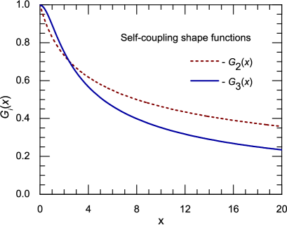
Figure 4: (Color online.) The graph of the self–coupling shape functions $G_{i}(x)$, $i$=2,3.

The shape functions obtained are (see Appendix B)

$$G_{2}(x)=2\dfrac{\sqrt{1+x}-1}{x}$$ (35)

for cubic self–coupling, and

$$G_{3}(x)=\dfrac{3}{2}\dfrac{\sqrt[3]{\sqrt{1+x^{2}}+x}-\sqrt[3]{\sqrt{1+x^{2}}-x}}{x}$$ (36)

for quartic selfinteractions. Both shape functions are normalized as $G_{i}(0)=1$, for $i=\{2,3\}$, and the graphs of them are shown in Fig. 4.

IV Applications and discussion

In preceding sections, we have mapped the DHF energy density in nuclear matter onto RMF–like functional with density–dependent effective couplings that are formally equivalent to the DHF approach with nonlinear self–couplings. The potential energy density of symmetric nuclear matter is finally written as

$$\left<\mathcal{V}\right>=-\frac{1}{2}\dfrac{\Gamma^{2}_{\sigma}}{m^{2}_{\sigma}}\rho^{2}_{S}+\frac{1}{2}\dfrac{\Gamma^{2}_{\omega}}{m^{2}_{\omega}}\rho^{2}_{B}\;,$$ (37)

where the density–dependent couplings now read

$$\frac{\Gamma_{\sigma}^{2}}{m_{\sigma}^{2}}=\frac{g_{\sigma}^{2}}{m_{\sigma}^{2}}G_{3(2)}(\beta_{\sigma}\rho_{S}) -\frac{1}{8}\frac{g_{\sigma}^{2}}{m_{\sigma}^{2}}G_{3(2)}(\beta_{\sigma}\rho_{S})X_{\theta}(k_{F}/m_{\sigma})+\frac{4}{8}\frac{g_{\omega}^{2}}{m_{\omega}^{2}}G_{3}(\beta_{\omega}\rho_{B})X_{\theta}(k_{F}/m_{\omega})+\frac{3}{8}\left(\frac{f_{\pi}}{m_{\pi}}\right)^{2}X_{\theta}(k_{F}/m_{\pi})$$

$$-\frac{2}{8}\frac{g_{\sigma}^{2}}{m_{\sigma}^{2}}G_{3(2)}(\beta_{\sigma}\rho_{S})X_{\phi}(k_{F}/m_{\sigma})-\frac{4}{8}\frac{g_{\omega}^{2}}{m_{\omega}^{2}}G_{3}(\beta_{\omega}\rho_{B})X_{\phi}(k_{F}/m_{\omega})+\frac{6}{8}\left(\frac{f_{\pi}}{m_{\pi}}\right)^{2}X_{\pi}(k_{F}/m_{\pi})\;,$$

and

$$\frac{\Gamma_{\omega}^{2}}{m_{\omega}^{2}}=\frac{g_{\omega}^{2}}{m_{\omega}^{2}}G_{3}(\beta_{\omega}\rho_{B}) +\frac{1}{8}\frac{g_{\sigma}^{2}}{m_{\sigma}^{2}}G_{3(2)}(\beta_{\sigma}\rho_{S})X_{\theta}(k_{F}/m_{\sigma})+\frac{2}{8}\frac{g_{\omega}^{2}}{m_{\omega}^{2}}G_{3}(\beta_{\omega}\rho_{B})X_{\theta}(k_{F}/m_{\omega})-\frac{3}{8}\left(\frac{f_{\pi}}{m_{\pi}}\right)^{2}X_{\theta}(k_{F}/m_{\pi})$$

$$-\frac{2}{8}\frac{g_{\sigma}^{2}}{m_{\sigma}^{2}}G_{3(2)}(\beta_{\sigma}\rho_{S})X_{\phi}(k_{F}/m_{\sigma})-\frac{4}{8}\frac{g_{\omega}^{2}}{m_{\omega}^{2}}G_{3}(\beta_{\omega}\rho_{B})X_{\phi}(k_{F}/m_{\omega})+\frac{6}{8}\left(\frac{f_{\pi}}{m_{\pi}}\right)^{2}X_{\pi}(k_{F}/m_{\pi})\;.$$

These expressions include both, the effect of Fock exchange via the exchange shape functions $X_{\theta}$, $X_{\phi}$ and $X_{\pi}$, and the medium modifications due to the nonlinear self–couplings via the shape functions $G_{i}$.

A few simple cases should be mentioned:

(a) Zero density constraints. The effective RMF couplings at zero density for both, the scalar and vector channels are constrained by simple relations to the DHF bare couplings. They are obtained by employing the values of shape functions at zero density. One may write

$$\left.\dfrac{\Gamma^{2}_{\sigma}}{m^{2}_{\sigma}}\right\rvert_{\rho_{B}=0}=\frac{7}{8}\dfrac{g_{\sigma}^{2}}{m_{\sigma}^{2}}+\frac{4}{8}\dfrac{g_{\omega}^{2}}{m_{\omega}^{2}}+\frac{3}{8}\left(\dfrac{f_{\pi}}{m_{\pi}}\right)^{2}\;,$$ (40)

and

$$\left.\dfrac{\Gamma^{2}_{\omega}}{m^{2}_{\omega}}\right\rvert_{\rho_{B}=0}=\frac{10}{8}\dfrac{g_{\omega}^{2}}{m_{\omega}^{2}}+\frac{1}{8}\dfrac{g_{\sigma}^{2}}{m_{\sigma}^{2}}-\frac{3}{8}\left(\dfrac{f_{\pi}}{m_{\pi}}\right)^{2}\;.$$ (41)

These relations demonstrate an important contribution of the $\omega$–meson exchange into both RMF effective couplings.

(b) No density dependence of exchange. The density dependence due to exchange correlations is relatively weak. Simple expressions for the effective couplings are obtained when it is already omitted, i.e. the exchange shape functions are replaced by their values at zero density, but keeping the self–interaction shape functions fully density–dependent. Then, the effective couplings read

$$\dfrac{\Gamma^{2}_{\sigma}}{m^{2}_{\sigma}}=\frac{7}{8}\dfrac{g_{\sigma}^{2}}{m_{\sigma}^{2}}G_{3(2)}(\beta_{\sigma}\rho_{S})+\frac{4}{8}\dfrac{g_{\omega}^{2}}{m_{\omega}^{2}}G_{3}(\beta_{\omega}\rho_{B})+\frac{3}{8}\left(\dfrac{f_{\pi}}{m_{\pi}}\right)^{2},$$ (42)

and

$$\dfrac{\Gamma^{2}_{\omega}}{m^{2}_{\omega}}=\frac{10}{8}\dfrac{g_{\omega}^{2}}{m_{\omega}^{2}}G_{3}(\beta_{\omega}\rho_{B})+\frac{1}{8}\dfrac{g_{\sigma}^{2}}{m_{\sigma}^{2}}G_{3(2)}(\beta_{\sigma}\rho_{S})-\frac{3}{8}\left(\dfrac{f_{\pi}}{m_{\pi}}\right)^{2}.$$ (43)

It is expected that the residual exchange density dependence is absorbed into the self–interaction density dependence parameters.

This model is close to the earlier developed density–dependent approaches (see e.g. [15, 16, 17, 18, 36] and references therein). Now, however, the compositions of effective mean–field couplings are dictated by the structure of exchange contributions, and the density dependence is induced by the nonlinear self–interactions.

(c) Low density limit. Previous results may be simplified further when the nuclear density of the system is relatively low. In such a case, the scalar density may be approximated by a scaled baryon density, i.e. $\rho_{S}\sim\rho_{B}$. Then the scalar density dependencies are replaced by the vector densities and the effective couplings take particularly simple forms,

$$\dfrac{\Gamma^{2}_{\sigma}}{m^{2}_{\sigma}}=\frac{7}{8}\dfrac{g_{\sigma}^{2}}{m_{\sigma}^{2}}G_{3(2)}(\beta^{\prime}_{\sigma}\rho_{B})+\frac{4}{8}\dfrac{g_{\omega}^{2}}{m_{\omega}^{2}}G_{3}(\beta_{\omega}\rho_{B})+\frac{3}{8}\left(\dfrac{f_{\pi}}{m_{\pi}}\right)^{2},$$ (44)

and

$$\dfrac{\Gamma^{2}_{\omega}}{m^{2}_{\omega}}=\frac{10}{8}\dfrac{g_{\omega}^{2}}{m_{\omega}^{2}}G_{3}(\beta_{\omega}\rho_{B})+\frac{1}{8}\dfrac{g_{\sigma}^{2}}{m_{\sigma}^{2}}G_{3(2)}(\beta^{\prime}_{\sigma}\rho_{B})-\frac{3}{8}\left(\dfrac{f_{\pi}}{m_{\pi}}\right)^{2}.$$ (45)

The model was used to fit the density–dependent vertices deduced from the Dirac–Brueckner–Hartree–Fock (DBHF) calculations of nuclear matter [19] with Bonn A interaction. The DHF coupling–to–mass ratios, $g^{2}_{\sigma}/m^{2}_{\sigma}$ and $g^{2}_{\omega}/m^{2}_{\omega}$, and the $\beta$’s were taken as free parameters of the fits. The DBHF vertices and the effective RMF fitting curves are compared in Fig. 5. The agreement is very good over the wide density region fitted despite the fact that only baryon density dependence of both effective couplings was used.

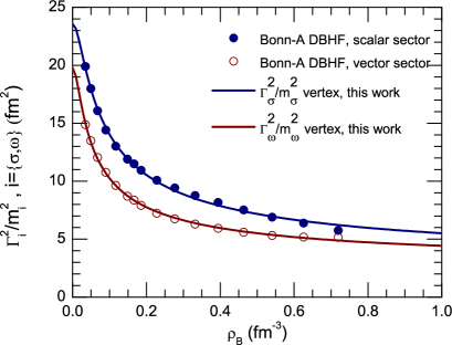
Figure 5: (Color online.) Density–dependent effective couplings. The solid and opens symbols were deduced from DBHF scalar and vector potentials, respectively, of the Brockmann and Machleidt calculations [19] for symmetric nuclear matter with Bonn A NN interaction. The solid lines are the fits employing the density–dependent self–coupling shape functions.

V Summary and conclusions

In the first part of the present work, we have mapped out the exchange Fock contributions of the DHF approach for symmetric nuclear matter onto the direct Hartree terms. This results in the effective relativistic mean–field model with the density–dependent (Fermi momentum–dependent) couplings. The density dependence of the coupling constants reflects the exchange correlations.

The approach is based upon the evaluation of exchange integrals of the DHF energy density components. All of them are expressed in the closed form via relevant densities and introduce no new parameters. Thus, it presents a step towards the formulation of the nonlocal Dirac–Hartree–Fock model as the local density functional theory. The exchange shape functions were derived that govern the $k_{F}$ dependence of Fock contributions.

The approach was tested against the DHF calculation of nuclear matter. It was shown that the effective RMF model reproduces well the DHF results for binding energy.

Alternatively, the approach may be developed by evaluating the exchange integrals in the relations for DHF self–energy components [39]. However, proceeding in this way we need to eliminate the momentum dependence of the exchange terms that is an inherent feature of the relativistic Hartree–Fock model. That was done by averaging the terms over the Fermi sphere. Contrary, no such approximations were introduced in the present work starting from exchange energy densities. Simply the $k$–dependence is internally integrated out.

It was observed that the density dependence of Fock exchange terms is relatively weak. Therefore, the nonlinear self–coupling terms were added to the DHF model. This leads to an additional density dependence of the effective RMF vertices that is decoupled from the Fock ones.

In the standard RMF model alone the scalar and vector self–interactions contribute only to the corresponding scalar or vector channels, respectively. The density dependence of the respective channel is thus fully determined by the given self–interaction only, and governed by the phenomenological ad–hoc parameterizations.

The model presented in this work exhibits a more complex density dependence. The scalar and vector self–interactions contribute coherently to the density dependence of both, the scalar and vector channels, together with a small tuning due to the exchange density dependencies.

While this work is restricted to the exchange of $\sigma$–, $\omega$–, and $\pi$–mesons only, the approach itself can be straightforwardly generalized for the full set of mesons, and for asymmetric nuclear matter. The contribution of this work is, we believe, a step in a direction to formulate the effective nuclear density functional suitable for the description of a wide class of nuclear phenomena over a broad range of densities. Such a development is of utmost importance since the theory is needed able to predict nuclear properties in regions of the nuclear chart not yet accessible to experiment. It seems that the relativistic self–consistent mean–field model with the density–dependent couplings, the structure and density dependence of which come from the nonlinear DHF theory, is a good approach to reach this goal.

Appendix A Evaluation of exchange integrals

By inspecting the DHF expression for the exchange energy density, Eq. (II), one reveals that it depends crucially only on a few kinds of exchange integrals without an apparent density dependence. Usually, they were evaluated numerically.

In this section we will give a detailed procedure for evaluating all types of exchange integrals of the DHF approach. The goal is to express them explicitly in the form of density–dependent terms.

A.1 The $A$–term integrals

The basic exchange integral over $A$–function dependent terms reads

$$I^{A}=\frac{g^{2}}{(2\pi)^{4}}\int_{0}^{k_{F}}k\,dk\int_{0}^{k_{F}}\Theta(k,q)\,q\,dq\;,$$ (46)

where $k_{F}$ is the nucleon Fermi momentum in nuclear matter, and the function $\Theta(k,q)$ is written as (see Eq. (18))

$$\Theta(k,q)=\ln\frac{(k+q)^{2}+m^{2}}{(k-q)^{2}+m^{2}}\;.$$ (47)

It depends on the mass of exchanged meson $m$ and the square of meson coupling $g^{2}$. Other numerical multiplicative factors were omitted to keep the integral as simple as possible.

This integral may be evaluated in the closed form. After some algebra, by employing the expression for a nucleon vector (baryon) density,

$$\rho_{B}(k_{F})=\frac{2}{3\pi^{2}}k_{F}^{3}\;,$$ (48)

the integral may be finally written in a compact form as

$$I^{A}=\frac{1}{16}\frac{g^{2}}{m^{2}}X_{\theta}(k_{F}/m)\rho_{B}^{2}(k_{F})\;,$$ (49)

where the auxiliary exchange shape function $X_{\theta}(x)$ is introduced. It reads

$$X_{\theta}(x) = \frac{3}{32}\left[4x^{2}\left(6x^{2}-1-8x\arctan 2x\right)\right.$$ (50)

$$+\left.\left(12x^{2}+1\right)\ln(1+4x^{2})\right]/x^{6}\;.$$

Here the $X_{\theta}(0)=1$ normalization was chosen. The graph of the function is plotted in Fig. 1.

A.2 The $B$–function integrals

The $B$–function exchange integrals are similar as the $A$–function ones, except they contains the $\hat{M}$ quantities. Namely, the integral take the basic form

$$I^{B}=\frac{g^{2}}{(2\pi)^{4}}\int_{0}^{k_{F}}\hat{M}(k)k\,dk\int_{0}^{k_{F}}\hat{M}(q)\Theta(k,q)q\,dq\;,$$ (51)

where

$$\hat{M}(k)=\frac{M^{*}(k)}{E^{*}(k)}\;,$$ (52)

and the quantities $M^{*}(k)$, $E^{*}(k)$ are the $k$–dependent effective mass and Fermi energy, respectively.

To proceed further, we firstly rewrite the $A$–function integral (A1) in an equivalent form as

$$I^{A}=\dfrac{g^{2}}{16}\int_{0}^{k_{F}}\dfrac{2}{\pi^{2}}k^{2}dk\int_{0}^{k_{F}}\left\{\frac{\Theta(k,q)}{4kq}\right\}\dfrac{2}{\pi^{2}}q^{2}dq\;.$$ (53)

Then, by applying the mean value theorem, the integral may be rewritten as

$$I^{A}=\frac{g^{2}}{16}K\int_{0}^{k_{F}}\dfrac{2}{\pi^{2}}k^{2}dk\int_{0}^{k_{F}}\dfrac{2}{\pi^{2}}q^{2}dq\;,$$ (54)

where

$$K=\left.\frac{\Theta(k,q)}{4kq}\right|_{k=\overline{s},q=\overline{s}}\;,$$ (55)

is evaluated at some intermediate point $\overline{s}$ of the integrating interval $\left(0,k_{F}\right>$. The remaining double integral results to the square of baryon density, $\rho_{B}$. The actual value of the quantity $K$ is then obtained by comparison with the relation (49).

Then, by applying this procedure for an evaluation of the $B$–function exchange integrals (51), one finally obtains the resulting expression,

$$I^{B}=\frac{1}{16}\frac{g^{2}}{m^{2}}X_{\theta}(k_{F}/m)\rho_{S}^{2}(k_{F},M^{\star})\;,$$ (56)

where $\rho_{S}$ is the scalar density and $M^{\star}$ is the effective nucleon mass.

A.3 The $C$–function integrals

The exchange integrals containing the $C$–term vertex functions are a bit more complicated than in previous cases. The form of integral depends upon the type of interaction.

For $\sigma$ and $\omega$ meson fields with direct (Yukawa) couplings to the nucleon field the basic integral is

$$I^{C}=\frac{g^{2}}{(2\pi)^{4}}\int_{0}^{k_{F}}\hat{P}(k)k\,dk\int_{0}^{k_{F}}\hat{P}(q)\Phi(k,q)q\,dq\;,$$ (57)

where $\Phi(k,q)$ is an angular exchange integral (see Eq. (19),

$$\Phi(k,q)=\frac{1}{4kq}(k^{2}+q^{2}+m^{2})\Theta(k,q)-1\;,$$ (58)

and

$$\hat{P}(k)=\frac{k^{\star}(k)}{E^{\star}(k)}\;.$$ (59)

To evaluate the $I^{C}$ integral we will employ the techniques used for the A– and B–functions cases. Firstly, we set $\hat{P}(k)\equiv 1$ in the integral (57). In this case the integral can be evaluated in the closed form,

$$\left.I^{C}\right|_{\hat{P}\equiv 1}=\frac{1}{16}\frac{g^{2}}{m^{2}}X_{\phi}(k_{F}/m)\rho_{B}^{2}(k_{F})\;,$$ (60)

where the exchange shape function $X_{\phi}$ is,

$$X_{\phi}(x)=\frac{-3}{16}\left[2x^{4}+\left(x^{2}+1\right)\left(16x\arctan x-8\arctan 2x\right.\right.$$

$$\left.\left.+4(x^{2}-1)\ln(1+x^{2})+(1-4x^{2})\ln(1+4x^{2})\right)\right]/x^{6}\;.$$

Subsequently, using the mean value theorem (as in the case of B–term integrals) and employing the on–shell condition, the C–term integral may be finally expressed as,

$$I^{C}=\frac{1}{16}\frac{g^{2}}{m^{2}}X_{\phi}(k_{F}/m)\left(\rho_{B}^{2}(k_{F})-\rho_{S}^{2}(k_{F},M^{\star})\right)\,.$$ (62)

The C–type function for the pion with a pseudovector coupling is given by a different expression (see Table 1),

$$C_{\pi}(k,q)=6\left(\dfrac{f_{\pi}}{m_{\pi}}\right)^{2}\left[\left(k^{2}+q^{2}\right)\Phi_{\pi}-kq\Theta_{\pi}\right]\;.$$ (63)

The exchange integral $I^{C}_{\pi}$ to be evaluated is

$$I^{C}_{\pi}=\dfrac{1}{(2\pi)^{4}}\int_{0}^{k_{F}}k\,dk\int_{0}^{k_{F}}C_{\pi}(k,q)q\,dq\;.$$ (64)

Proceed in an analogical way as in the previous case we write the $I^{C}_{\pi}$ integral in the closed form

$$I^{C}_{\pi}=\frac{6}{16}\left(\dfrac{f_{\pi}}{m_{\pi}}\right)^{2}X_{\pi}(k_{F}/m_{\pi})\left(\rho_{B}^{2}(k_{F})-\rho_{S}^{2}(k_{F},M^{\star})\right)\;,$$ (65)

where the exchange shape fubction $X_{\pi}$ is written as

$$X_{\pi}(x)=\frac{-1}{80}\left[56x^{6}+18x^{4}+\left(40x^{3}-24x\right)\left(2\arctan x\right.\right.$$

$$\left.\left.-\arctan 2x\right)-\left(16x^{6}+60x^{4}+5\right)\left(\ln(1+4x^{2})\right.\right.$$

$$\left.\left.-\ln(1+x^{2})\right)+15\ln(1+x^{2})\right]/x^{6}\;.$$ (66)

The graphs of both shape functions, $X_{\phi}$ and $X_{\pi}$, are also shown in Fig. 1.

Appendix B Self–coupling shape functions

The meson field equations reduce in nuclear matter to simple algebraic equations,

$$u=a(\rho-cu^{n})\;,\quad n=\{2,3\}\;,$$ (67)

where $u$ is a meson potential, $\rho$ is the source density, and the real constants $a$ and $c$ mean the coupling and self–coupling strengths. The exponent $n$ takes the value 2 or 3, depending upon the cubic or quartic self–coupling terms in the model Lagrangian density, respectively. The solutions of (67) are usually obtained in a direct way or iteratively.

For the approach developed in this paper it is of advantage to express the solutions in the form

$$u=a\,G(\beta\rho)\,\rho\;,$$ (68)

which resembles the solution of linear model. We are interested in real solutions with the normalization $G(0)=1$. The effect of self–couplings is hidden within the density–dependence of the self–coupling shape function $G$, and the factor $\beta$ is the new self–coupling strength. It can be expressed using the constants $a$ and $c$ of (67) (e.g. $\beta=4a^{2}c$ for the cubic self–interaction, and $\beta=\sqrt{27a^{3}c}/2$ for quartic one, respectively). We expect, however, that in most cases the values of $\beta$’s to be determined in the model parameter optimization procedure.

The explicit form of the shape function is

$$G_{2}(x)=2\dfrac{\sqrt{1+x}-1}{x}\;,$$ (69)

for the cubic self–interaction, and

$$G_{3}(x)=\dfrac{3}{2}\dfrac{\sqrt[3]{\sqrt{1+x^{2}}+x}-\sqrt[3]{\sqrt{1+x^{2}}-x}}{x}\;,$$ (70)

for the quartic self–coupling. The shape function graphs are shown in Fig. 4.

References

- Hohenberg and Kohn [1964] P. Hohenberg and W. Kohn, Phys. Rev. 136, B864 (1964).
- Kohn and Sham [1965] W. Kohn and L. J. Sham, Phys. Rev. 140, A1133 (1965).
- Speicher et al. [1992] C. Speicher, R. Dreizler, and E. Engel, Annals of Physics 213, 312 (1992).
- Schmid et al. [1995a] R. N. Schmid, E. Engel, and R. M. Dreizler, Phys. Rev. C 52, 164 (1995a).
- Schunck [2019] N. Schunck, ed., Energy Density Functional Methods for Atomic Nuclei, 2053-2563 (IOP Publishing, 2019).
- Meng [2016] J. Meng, Relativistic Density Functional for Nuclear Structure, International Review of Nuclear Physics (World Scientific Publishing Company, 2016).
- Lalazissis et al. [2004] G. Lalazissis, P. Ring, and D. Vretenar, Extended Density Functionals in Nuclear Structure Physics, Lecture Notes in Physics (Springer Berlin Heidelberg, 2004).
- Miller and Green [1972] L. D. Miller and A. E. S. Green, Phys. Rev. C 5, 241 (1972).
- Walecka [1974] J. Walecka, Ann. Phys. (N.Y.) 83, 491 (1974).
- Bender et al. [2003] M. Bender, P.-H. Heenen, and P.-G. Reinhard, Rev. Mod. Phys. 75, 121 (2003).
- Boguta and Bodmer [1977] J. Boguta and A. Bodmer, Nucl. Phys. A 292, 413 (1977).
- Bodmer [1991] A. Bodmer, Nucl. Phys. A 526, 703 (1991).
- Gmuca [1992] S. Gmuca, Nucl. Phys. A 547, 447 (1992).
- Mueller and Serot [1996] H. Mueller and B. D. Serot, Nucl. Phys. A 606, 508 (1996).
- Fuchs et al. [1995] C. Fuchs, H. Lenske, and H. H. Wolter, Phys. Rev. C 52, 3043 (1995).
- Typel and Wolter [1999] S. Typel and H. Wolter, Nucl. Phys. A 656, 331 (1999).
- Shen et al. [1997] H. Shen, Y. Sugahara, and H. Toki, Phys. Rev. C 55, 1211 (1997).
- Hofmann et al. [2001] F. Hofmann, C. M. Keil, and H. Lenske, Phys. Rev. C 64, 034314 (2001).
- Brockmann and Machleidt [1990] R. Brockmann and R. Machleidt, Phys. Rev. C 42, 1965 (1990).
- Huber et al. [1995] H. Huber, F. Weber, and M. K. Weigel, Phys. Rev. C 51, 1790 (1995).
- Alonso and Sammarruca [2003] D. Alonso and F. Sammarruca, Phys. Rev. C 67, 054301 (2003).
- van Dalen et al. [2004] E. van Dalen, C. Fuchs, and A. Faessler, Nucl. Phys. A 744, 227 (2004).
- Katayama and Saito [2013] T. Katayama and K. Saito, Phys. Rev. C 88, 035805 (2013).
- Petrík and Gmuca [2012] K. Petrík and S. Gmuca, J. Phys. G: Nucl. Part. Phys. 39, 085113 (2012).
- Horowitz and Serot [1983] C. Horowitz and B. D. Serot, Nucl. Phys. A 399, 529 (1983).
- Bouyssy et al. [1987] A. Bouyssy, J.-F. Mathiot, N. Van Giai, and S. Marcos, Phys. Rev. C 36, 380 (1987).
- Fritz et al. [1993] R. Fritz, H. Müther, and R. Machleidt, Phys. Rev. Lett. 71, 46 (1993).
- Shi et al. [1995] H.-L. Shi, B.-Q. Chen, and Z.-Y. Ma, Phys. Rev. C 52, 144 (1995).
- Jaminon et al. [1981] M. Jaminon, C. Mahaux, and P. Rochus, Nucl. Phys. A 365, 371 (1981).
- Schmid et al. [1995b] R. N. Schmid, E. Engel, and R. M. Dreizler, Phys. Rev. C 52, 2804 (1995b).
- Greco et al. [2001] V. Greco, F. Matera, M. Colonna, M. Di Toro, and G. Fabbri, Phys. Rev. C 63, 035202 (2001).
- Giai et al. [2010] N. V. Giai, B. V. Carlson, Z. Ma, and H. Wolter, J. Phys. G: Nucl. Part. Phys. 37, 064043 (2010).
- Horowitz and Serot [1982] C. Horowitz and B. D. Serot, Phys. Lett. B 109, 341 (1982).
- Bouyssy et al. [1985] A. Bouyssy, S. Marcos, J. F. Mathiot, and N. Van Giai, Phys. Rev. Lett. 55, 1731 (1985).
- Note [1] In fact, Fermi momentum dependence. However, as of a definite relation between and , we will often use the terms “Fermi momentum–dependent”and “density–dependent”interchangeably.
- Typel [2018] S. Typel, Particles 1, 3 (2018).
- Horowitz and Piekarewicz [2001] C. J. Horowitz and J. Piekarewicz, Phys. Rev. Lett. 86, 5647 (2001).
- Bernardos et al. [1993] P. Bernardos, V. N. Fomenko, N. V. Giai, M. L. Quelle, S. Marcos, R. Niembro, and L. N. Savushkin, Phys. Rev. C 48, 2665 (1993).
- Gmuca et al. [2019] S. Gmuca, K. Petrík, and J. Leja, EPJ Web Conf. 204, 05001 (2019).