In this manuscript, we develop an efficient algorithm to evaluate the azimuthal Fourier components of the Green’s function for the Helmholtz equation in cylindrical coordinates. A computationally efficient algorithm for this modal Green’s function is essential for solvers for electromagnetic scattering from bodies of revolution (e.g., radar cross sections, antennas). Current algorithms to evaluate this modal Green’s function become computationally intractable when the source and target are close or when the wavenumber is large. Furthermore, most state of the art methods cannot be easily parallelized. In this manuscript, we present an algorithm for evaluating the modal Green’s function that has performance independent of both source-to-target proximity and wavenumber, and whose cost grows as $O(m)$, where $m$ is the Fourier mode. Furthermore, our algorithm is embarrassingly parallelizable.

On the Efficient Evaluation of the Azimuthal Fourier Components of the Green’s Function for Helmholtz’s Equation in Cylindrical Coordinates

James Garritano$\mbox{}^{\ast\,\sharp\,\otimes}$, Yuval Kluger$\mbox{}^{\ast\,\sharp}$,

Vladimir Rokhlin$\mbox{}^{\ast\,\ddagger\,\oplus}$, Kirill Serkh$\mbox{}^{\dagger\,\diamond}$

$\mbox{}^{\otimes}$ This author’s work was supported in part by NIH F30HG011193 and by US NIH MSTP Training Grant T32GM007205.
$\mbox{}^{\oplus}$ This author’s work was supported in part by ONR N00014-18-1-2353 and NSF DMS-1952751.
$\mbox{}^{\diamond}$ This author’s work was supported in part by the NSERC Discovery Grants RGPIN-2020-06022 and DGECR-2020-00356.

$\mbox{}^{\ast}$ Program in Applied Mathematics, Yale University, New Haven, CT 06511
$\mbox{}^{\sharp}$ Yale School of Medicine, New Haven, CT 06511
$\mbox{}^{\ddagger}$ Dept. of Mathematics, Yale University, New Haven, CT 06511
$\mbox{}^{\dagger}$ Dept. of Math. and Computer Science, University of Toronto, Toronto, ON M5S 2E4

1 Introduction

This manuscript will detail how to efficiently compute the azimuthal Fourier components of the Green’s function (i.e., the modal Green’s functions) for the Helmholtz equation in three dimensions, known to be

$$G_{m}(\bm{x},\bm{x}^{\prime})=G_{m}(|\bm{x}-\bm{x}^{\prime}|)=\frac{1}{2\pi}\int_{-\pi}^{\pi}\frac{1}{4\pi}\frac{e^{ik|\bm{x}-\bm{x}^{\prime}|}}{|\bm{x}-\bm{x}^{\prime}|}e^{-im\theta}d\theta,$$ (1)

where $\bm{x},\bm{x^{\prime}}\in\mathbb{R}^{3}$, $k$ is the wavenumber, and $m$ is the $m$th azimuthal Fourier mode. Rewriting this equation in cylindrical coordinates, with $\bm{x}=(r,\theta,z)$ and $\bm{x^{\prime}}=(r^{\prime},\theta^{\prime},z^{\prime})$, and letting $\phi=\theta-\theta^{\prime}$, the formula for the $m$th Fourier coefficient becomes

$$G_{m}(\bm{x},\bm{x}^{\prime})=\frac{1}{4\pi^{2}R_{0}}\int_{0}^{\pi}\frac{e^{-i\kappa\sqrt{1-\alpha\cos\phi}}}{\sqrt{1-\alpha\cos\phi}}\cos{m\phi}d\phi,$$ (2)

where $\kappa=kR_{0}$, $\alpha=2rr^{\prime}/R_{0}^{2}$, and $R_{0}^{2}=r^{2}+r^{\prime 2}+(z-z^{\prime})^{2}$.

This integral has two features which make numeric integration difficult: the integrand is oscillatory, and it is near-singular when the distance between $\bm{x}$ and $\bm{x^{\prime}}$ is small (i.e., as $\alpha$ approaches 1). However, the integrand vanishes for sufficiently large imaginary values of $\kappa$, suggesting that Cauchy’s theorem can be used to construct a contour on which all the oscillations occur where the integrand is negligible.

When devising an appropriate contour, it is helpful to consider three cases: 1) when $\kappa$ is zero and $m\geq 0$, 2) when $\kappa$ is arbitrary and $m$ is small, and 3) when both $\kappa$ and $m$ are large.

Determining the appropriate contour when $\kappa=0$ and $m\geq 0$ (when the Helmholtz equation becomes the Laplace equation) is trivial, because on any vertical contour (into quadrant IV of the complex plane) the integrand monotonically decays. When $\kappa>0$ and $m=1$, the appropriate contours were solved by Gustafsson [11] via the method of steepest descent. However, Gustafsson did not analyze cases where both $\kappa>0$ and $m>1$. In fact, when both $m$ and $\kappa$ are large, it turns out that no contour exists on which the entire integrand monotonically decays.

We develop on Gustafsson’s work by integrating along the contour on which the spherical wave component,

$$\frac{e^{-i\kappa\sqrt{1-\alpha\cos\phi}}}{\sqrt{1-\alpha\cos\phi}},$$ (3)

monotonically decays. However, the part of the integrand dependent on azimuthal frequency, $\cos(m\phi)$, behaves poorly and grows on this contour. To circumvent this behavior, we replace the term $\cos(m\phi)$ with a rational function approximation which does not grow in the complex plane. The growth of $\cos(m\phi)$ along the contour is subsumed in a collection of residues which must be added to the resulting integral.

1.1 The Modal Green’s Functions for the Helmholtz Equation

The Green’s function for the Helmholtz equation in three dimensions satisfies the equation

$$(\nabla^{2}+k^{2})G_{k}(\bm{x},\bm{x}^{\prime})=\delta(\bm{x}-\bm{x}^{\prime}),$$ (4)

where k is the wave number and $\bm{x}$, $\bm{x^{\prime}}\in\mathbb{R}^{3}$. The solution is an outgoing spherical wave, given by the formula

$$G_{k}(\bm{x},\bm{x}^{\prime})=G_{k}(|\bm{x}-\bm{x}^{\prime}|)=\frac{1}{4\pi}\frac{e^{ik|\bm{x}-\bm{x}^{\prime}|}}{|\bm{x}-\bm{x}^{\prime}|}.$$ (5)

We consider a problem with rotational symmetry (i.e., a body of revolution). Switching to cylindrical coordinates and expanding $G_{k}$ in Fourier series, we have

$$G_{k}(\bm{x},\bm{x}^{\prime})=\sum_{m=-\infty}^{\infty}G_{m,k}(r,z,r^{\prime},z^{\prime})e^{im(\theta-\theta^{\prime})},$$ (6)

where $\bm{x}=(r,\theta,z)$, $\bm{x^{\prime}}=(r^{\prime},\theta^{\prime},z^{\prime})$. Let $\phi=\theta-\theta^{\prime}$ denote the difference in azimuthal angles. The formula for the $m$th coefficient is

$$G_{m,k}(r,z,r^{\prime},z^{\prime})=\frac{1}{2\pi}\int_{-\pi}^{\pi}G_{k}(r,z,r^{\prime},z^{\prime},\phi)e^{-im\phi}d\phi.$$ (7)

We adopt notation consistent with the literature (see, for example, [7, 9, 23]) and omit the subscript $k$ denoting the wavenumber. Expanding the representation for the $m$th Fourier coefficient, we have

$$G_{m}(r,z,r^{\prime},z^{\prime})=\frac{1}{2\pi}\int_{-\pi}^{\pi}\frac{e^{ik\sqrt{r^{2}+r^{\prime 2}-2rr^{\prime}\cos\phi+(z-z^{\prime})^{2}}}}{4\pi\sqrt{r^{2}+r^{\prime 2}-2rr^{\prime}\cos\phi+(z-z^{\prime})^{2}}}e^{-im\phi}d\phi.$$ (8)

We then introduce the parameter $R_{0}$, given by

$$R_{0}=\sqrt{r^{2}+r^{\prime 2}+(z-z^{\prime})^{2}},$$ (9)

which we use to rewrite (8), by defining $\kappa=kR_{0}$ and $\alpha=2rr^{\prime}/R_{0}^{2}$, obtaining

$$G_{m}(\bm{x},\bm{x}^{\prime})=\frac{1}{8\pi^{2}R_{0}}\int_{-\pi}^{\pi}\frac{e^{i\kappa\sqrt{1-\alpha\cos\phi}}}{\sqrt{1-\alpha\cos\phi}}e^{-im\phi}d\phi.$$ (10)

Any numerical scheme for evaluating $G_{m}$ must depend on four parameters: $\kappa$, $\alpha$, $R_{0}$, and $m$. Notably, $\alpha$ is bounded by $0\leq\alpha<1$, and determines the growth of the integrand near $\phi=0$. In Section 3.6, we will introduce the parameters $\beta_{-}$ and $\beta_{+}$, defined to be

$$\beta_{-}=\sqrt{1/\alpha-1},\qquad\beta_{+}=\sqrt{1/\alpha+1}.$$ (11)

We also introduce the parameters $\Delta$ and $\rho_{0}$, defined as

$$\Delta =\sqrt{(r-r^{\prime})^{2}+(z-z^{\prime})^{2}},$$ (12)

$$\rho_{0} =2rr^{\prime}.$$ (13)

Note that $\Delta$ is the minimum distance between the source and the target, $R_{0}$ is the maximum distance between the source and the target, and that $\Delta^{2}=R_{0}^{2}-\rho_{0}$ . Lastly, we observe that $\beta_{-}$ and $\beta_{+}$ also given by the formulae,

$$\beta_{-}=\frac{\Delta}{\rho_{0}},\qquad\beta_{+}=\sqrt{\frac{R_{0}^{2}+\rho_{0}}{\rho_{0}}}.$$ (14)

We note that numerically computing $\beta_{-}$ from $\alpha$ using (11) will result in cancellation error when $\alpha\approx 1$, so it is usually better to compute $\beta_{-}$ directly from formula (14).

A representative sample of the literature related to the evaluation of the modal Green’s functions can be found in [1, 3, 6, 8, 9, 10, 12, 14, 15, 17, 21].

1.1.1 Number of Fourier Coefficients Needed

Matviyenko in [17] derived an upper bound, $r_{+}$, such that all Fourier modes $m>r_{+}$ geometrically decay as $m$ increases, with $r_{+}$ given by

$$r_{+}=\frac{\kappa}{\sqrt{2}}\sqrt{1+\sqrt{1-\alpha^{2}}},$$ (15)

where $\alpha=\rho_{0}/R_{0}^{2}$ and $\kappa=kR_{0}$ (see [17], formulae (37) and (38)). When $\alpha\approx 1$, formula (15) simplifies to

$$r_{+}\approx\frac{\kappa}{\sqrt{2}}.$$ (16)

Using Matviyenko’s formula for the decay of the modal Green’s functions (see [17], formula (40)), it can be shown that the magnitude of any Fourier coefficient $m>r_{+}$ is bounded by

$$|G_{m}|<|G_{\lfloor r_{+}\rfloor}|\Bigg{(}\frac{\sqrt{1-\sqrt{1-\alpha^{2}}}}{\sqrt{1+\sqrt{1-\alpha^{2}}}}\Bigg{)}^{m-\lfloor r_{+}\rfloor}.$$ (17)

Substituting $\alpha=1/(\beta_{-}^{2}+1)$ into (17), this bound can be simplified to

$$|G_{m}|<|G_{\lfloor r_{+}\rfloor}|\Bigg{(}1-\frac{\beta_{-}\sqrt{\beta_{-}^{2}+2}}{1+\beta_{-}^{2}}\Bigg{)}^{\frac{m-\lfloor r_{+}\rfloor}{2}}\Bigg{(}1+\frac{\beta_{-}\sqrt{\beta_{-}^{2}+2}}{1+\beta_{-}^{2}}\Bigg{)}^{-\frac{m-\lfloor r_{+}\rfloor}{2}},$$ (18)

where $\beta_{-}$ is the scaled source-to-target distance. When $\beta_{-}$ is small, $1+\beta_{-}^{2}\approx 1$, and (18) can be approximated as

$$|G_{m}|\lesssim|G_{\lfloor r_{+}\rfloor}|\Bigg{(}\frac{1-\beta_{-}\sqrt{2}}{1+\beta_{-}\sqrt{2}}\Bigg{)}^{\frac{m-\lfloor r_{+}\rfloor}{2}}\approx|G_{\lfloor r_{+}\rfloor}|(1-\beta_{-}2\sqrt{2})^{\frac{m-\lfloor r_{+}\rfloor}{2}},$$ (19)

where we have replaced the exponentiated term with its truncated Taylor expansion in $\beta_{-}$. Formula (19) can be used to determine the Fourier mode $M$ such that for $m>M$, $|G_{m}|<\epsilon$, where $M$ is given by

$$M\approx\frac{2\log(\epsilon)-2\log{(|G_{\lfloor r_{+}\rfloor}|)}}{\log(1-2\sqrt{2}\beta_{-})}+\lfloor r_{+}\rfloor.$$ (20)

By substituting (15) into (20, we can characterize the order of $M$ as a function of $\beta_{-}$ and $\kappa$ when the source and target are close (i.e., $\alpha\gtrsim 0.99$ or equivalently $\beta_{-}\lesssim 10^{-2}$) as

$$\begin{split}M\approx&\frac{2\log(\epsilon)-2\log{(|G_{\lfloor r_{+}\rfloor}|)}}{\log(1-2\sqrt{2}\beta_{-})}+\frac{\kappa}{\sqrt{2}}\\ =&\bigg{(}1-\frac{1}{\sqrt{2}\beta_{-}}\bigg{)}\big{(}\log(\epsilon)-\log{(|G_{\lfloor r_{+}\rfloor}|}\big{)}+\,\frac{\kappa}{\sqrt{2}}+O(\beta_{-}^{2})\\ =&O\Big{(}\frac{1}{\beta_{-}}+\kappa\Big{)},\end{split}$$ (21)

where we have replaced the denominator of (20) with its Taylor expansion in $\beta_{-}$. Lastly, it is often useful to write (21) in terms of the radius of the body of revolution and the minimum source-to-target distance, $\Delta$. We rewrite (21) as

$$M=O\Big{(}\frac{\rho_{0}}{\Delta}+k\sqrt{\rho_{0}+\Delta^{2}}\Big{)},$$ (22)

where we have substituted $\kappa=kR_{0}$ and $\beta_{-}=\rho_{0}/\Delta$. Because $\Delta^{2}\ll\rho_{0}$,

$$M=O\Big{(}\frac{\rho_{0}}{\Delta}+k\sqrt{\rho_{0}}\Big{)}.$$ (23)

Recall that $\rho_{0}=2rr^{\prime}$. When $\Delta$ is very small, $2rr^{\prime}\approx 2r^{2}$, meaning that formula (23) becomes

$$M=O\Big{(}\frac{2r^{2}}{\Delta}+kr\sqrt{2}\Big{)}=O\Big{(}\frac{r^{2}}{\Delta}+kr\Big{)}.$$ (24)

1.1.2 Informal Description of the Spectra of the Green’s Functions

The Green’s function for the Helmholtz equation in cylindrical coordinates,

$$G(\bm{x},\bm{x}^{\prime})=\frac{e^{i\kappa\sqrt{1-\alpha\cos\phi}}}{\sqrt{1-\alpha\cos\phi}},$$ (25)

can be viewed as the product of the Green’s function for the Laplace equation,

$$G^{L}(\bm{x},\bm{x}^{\prime})=\frac{1}{\sqrt{1-\alpha\cos\phi}},$$ (26)

with the band-limited term $\exp(i\kappa R(\theta))$, where $R=\sqrt{1-\alpha\cos\phi}$, $\bm{x}=(r,\theta,z)$, $\bm{x^{\prime}}=(r^{\prime},\theta^{\prime},z^{\prime})$, $\phi=\theta-\theta^{\prime}$, $\alpha=2rr^{\prime}/R_{0}^{2}$, and $\kappa=kR_{0}$, where $G$ and $G_{L}$ are understood to be a functions of $\kappa$, $\alpha$, and $R_{0}$.

Recall that the Fourier transform of the product of two functions is the convolution of their Fourier transforms. Hence, the modal Green’s function can be thought of as the convolution of the Fourier coefficients of $G^{L}(\bm{x},\bm{x}^{\prime})$ and the Fourier coefficients of $\exp(i\kappa R(\theta))$. Using this observation, combined with Matviyenko’s formulae for the cut-off frequency (formula (15)) and the rate of the decay of Fourier coefficients (formula (17)), we now provide a rough description of the spectra of the Green’s functions.

First, we describe the spectra of the Green’s functions of the Laplace equation. The Fourier coefficients of the Green’s functions of the Laplace equation decay as a function of $\alpha$, with the rate given by formula (17) (see Figure 1).

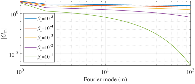
Figure 1: Spectra of the Green’s functions for the Laplace equation with varying source-to-target distance.

Now that we have characterized the spectra of the Green’s functions for the Laplace equation, we are ready to describe the spectra of the Green’s functions for the Helmholtz equation when $\kappa>0$. Recall that formula (15) provides a cut-off frequency $r_{+}$ such that, for $m>r_{+}$, $G_{m}$ geometrically decays; recall also that $r_{+}$ scales with $\kappa$ (see Figure 2). For all $m>r_{+}$, the rate of the decay of the Fourier coefficients is determined by the source-to-target distance by formula (17) (see Figure 3).

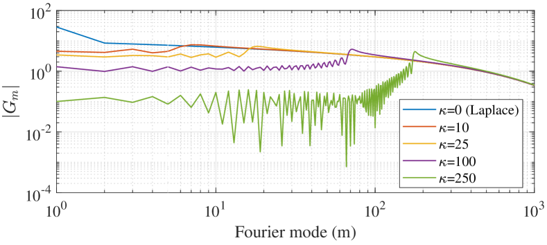
Figure 2: Spectra of the Green’s functions for the Helmholtz equation when the source and target are close with $\beta_{-}=10^{-3}$ and varying $\kappa$.

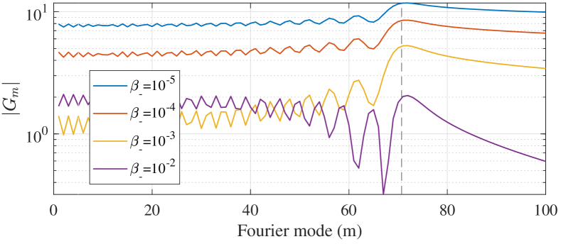
Figure 3: Spectra of the Green’s functions for the Helmholtz equation when the source and target are close for $\kappa=100$ with varying $\beta_{-}$. The approximation for the index $r_{+}$ after which the Fourier modes geometrically decay (given by formula (16)) is represented by a vertical dashed line.

1.2 Review of the Literature

Recall from Section 1.1 that the modal Green’s function is a function of three parameters: $\kappa$, $m$, and $\alpha$. We divide the literature on fast algorithms for evaluating the modal Green’s function into two categories: those that evaluate the general case of any combination of input parameters and those that evaluate special cases of input parameters (e.g., when the source and target are well-separated, when $m=1$, etc.).

Almost all modern fast general-case algorithms are based on the application of the Fast Fourier Transform (FFT) (see, for example, [9, 10, 13, 12, 14, 21, 22, 23]). In contrast, the special-case algorithms have a diverse set of methodologies which cannot easily be summarized. Because this manuscript’s topic is a general-case algorithm which works for all input parameters, we do not review the literature of special-case algorithms, with the exception of Gustfasson’s contour integration technique [11], which we develop on extensively in this manuscript.

1.2.1 Introduction to FFT-Based Kernel Splitting

Almost all published fast general-case algorithms for evaluating the modal Green’s functions (i.e., those that take as input an arbitrary source-to-target distance and arbitrary Fourier mode) use the Fast Fourier Transform (FFT). Because computing the Fourier coefficients of a near-singular function is not efficient, and because the Green’s function becomes near-singular for $\alpha\approx 1$ (i.e., when the source and target are close), all modern implementations of FFT-based methods employ kernel splitting, the technique of splitting the integrand into a near-singular portion and a non-singular portion, then computing each portion’s coefficient’s separately. For the non-singular portion, the FFT is often fast and efficient. For the near-singular portion, some other technique, usually a purpose-made recurrence relation, is used to evaluate the singular integral.

Two kernel splittings are used in the literature of FFT-based evaluations of the modal Green’s function: the splitting of Gedney and Mittra [10] (see, for example, [10, 21, 22]) and the splitting of Helsing [13] (see, for example, [9, 13, 14, 23]).

Gedney and Mittra in [10] isolate the near-singular portion of the integral by adding and subtracting a $1/R$ term, resulting in the splitting

$$\begin{split}G_{m}&=\int\frac{e^{-i\kappa\sqrt{1-\alpha\cos\phi}}}{\sqrt{1-\alpha\cos\phi}}+\frac{1}{\sqrt{1-\alpha\cos\phi}}-\frac{1}{\sqrt{1-\alpha\cos\phi}}d\phi\\ &=\underbrace{\int\frac{1}{\sqrt{1-\alpha\cos\phi}}d\phi}_{\small\text{ near-singular}}+\underbrace{\int\frac{e^{i\kappa\sqrt{1-\alpha\cos\phi}}-1}{\sqrt{1-\alpha\cos\phi}}d\phi}_{\small\text{non-singular, not very smooth}}.\end{split}$$ (27)

With this splitting, as $\alpha\to 1$, the near-singular term’s growth is unbounded, while the non-singular term’s growth is bounded. Although this splitting isolates the near-singular portion of the integral, the resulting non-singular integral is not very smooth as $\alpha\to 1$. Hence, directly applying the FFT to the non-singular portion remains inefficient when $\alpha\approx 1$, meaning that efficient evaluation of the non-singular term in (27) requires additional manipulation of the integrand.

Helsing in [13] split the integral via application of Euler’s formula, resulting in

$$\begin{split}G_{m}&=\int\frac{e^{-i\kappa\sqrt{1-\alpha\cos\phi}}}{\sqrt{1-\alpha\cos\phi}}d\phi\\ &=\underbrace{\int\frac{\cos(\sqrt{1-\alpha\cos\phi})}{\sqrt{1-\alpha\cos\phi}}d\phi}_{\small\text{ near-singular}}+\underbrace{\int\frac{i\sin(\sqrt{1-\alpha\cos\phi})}{\sqrt{1-\alpha\cos\phi}}d\phi}_{\small\text{ non-singular, smooth}}.\end{split}$$ (28)

In contrast to (27), the non-singular portion of formula (28) is smooth as $\alpha\to 1$. Consequently, the Fourier coefficients of the non-singular portion of (28) can be efficiently evaluated by the FFT.

Careful analysis of recent implementations of both kernel splitting techniques shows that the splitting of Helsing is sufficient to efficiently utilize the FFT to compute the modal Green’s function (see Section 1.2.2), while the splitting of Gedney and Mittra requires further techniques to evaluate the non-singular integral. In fact, the fastest algorithm utilizing the splitting of Gedney and Mittra, published by Vaessen et al. [21], split the non-singular integral again into a part which is smooth as $\alpha\to$ and a part which is not. It turns out that this final splitting is essentially equivalent to Helsing’s. Because the splitting of Helsing is utilized in the fastest algorithm for both techniques, we first summarize the splitting of Helsing by examining a recent fast implementation, then conclude our review by summarizing the fastest implementation of Gedney and Mittra’s splitting. Lastly, we demonstrate that it is algorithmically equivalent to the fastest implementation of Helsing’s splitting.

1.2.2 Method of Epstein et al., a Recent Implementation of Helsing’s Kernel Splitting

In Epstein et al. [9], the modal Green’s functions are computed using a Fast Fourier Transform (FFT)-based method, with the kernel splitting of Helsing [13]. In the following, the definitions for $m$, $\kappa$, $\alpha$, and $R_{0}$ are identical to those used in Section 1.1.

The authors divide the evaluation of the modal Green’s function for Fourier modes $-M,-M+1,\dots,M-1,M$ into two cases: one where the source and target are well-separated ($0\leq\alpha\leq 1/1.005$), and one where the source and target are close ($1/1.005\leq\alpha<1$).

In the former case, the integrand is relatively smooth, and the modal Green’s functions are computed using an $L$-point FFT, obtaining near double precision accuracy when $L\geq 4|\kappa|$. When $|\kappa|\leq 256$, a 1024 point FFT is used. The parameter $L$ must be chosen such that $L>2M$, but in practical situations $2M$ is usually smaller than the $L$ chosen via this heuristic.

For the near-singular case, $\alpha\approx 1$, the authors follow [13] by first rewriting (10) as

$$G_{m}(\bm{x},\bm{x}^{\prime})=\frac{1}{2\pi}\int_{-\pi}^{\pi}\frac{\cos(\kappa\sqrt{1-\alpha\cos\phi})+i\sin(\kappa\sqrt{1-\alpha\cos\phi})}{4\pi R_{0}\sqrt{1-\alpha\cos\phi}}e^{-im\phi}d\phi$$ (29)

(see [13] Section 3, formula (9)). The integrand of (29) is split into a smooth sine term, $H^{s}$, and a near-singular cosine term, $H^{c}$, where $H^{s}$ and $H^{c}$ are given by

$$H^{s}(\phi;\kappa,\alpha)=\frac{\sin(\kappa\sqrt{1-\alpha\cos\phi})}{\sqrt{1-\alpha\cos\phi}},\quad H^{c}(\phi;\kappa,\alpha)=\frac{\cos(\kappa\sqrt{1-\alpha\cos\phi})}{\sqrt{1-\alpha\cos\phi}}.$$ (30)

The Fourier modes of $H^{c}$ are computed as the linear convolution of the Fourier modes of $\cos(\kappa\sqrt{1-\alpha\cos\phi})$ and the Fourier modes of $1/\sqrt{1-\alpha\cos\phi}$. The Fourier modes of $\cos(\kappa\sqrt{1-\alpha\cos\phi})$ are computed via the FFT, while the Fourier modes of $1/\sqrt{1-\alpha\cos\phi}$ are known to be proportional to $Q_{m-1/2}(\chi)$ (see [7]), where $Q_{m-1/2}$ is the Legendre function of the second kind of half-order, with $\chi$ given by

$$\chi=\frac{r^{2}+r^{\prime 2}+(z-z^{\prime})^{2}}{2rr^{\prime}}=\frac{1}{\alpha}.$$ (31)

Note that $\chi\approx 1$ when $\alpha\approx 1$ (i.e., when the minimum distance between the source and target is very small). The authors complete their algorithm by computing $Q_{m-1/2}(\chi)$ via a recurrence, which has cost that grows as $O(1/\beta_{-})$, where $\beta_{-}=\Delta/\rho_{0}$. Thus, their recurrence has poor performance for $\chi\approx 1$ (i.e., when the target and source are close). We note that a fast algorithm was recently introduced by Bremer in [4], which evaluates $Q_{m-1/2}(\chi)$ in constant run-time independent of $m$. Bremer’s algorithm for evaluating the Legendre function of the second kind of half-order [4] is practically useful, not only as an improvement to [9], but as an ingredient in a potential $O(1)$ evaluator for an arbitrary mode of the Green’s function for the Laplace equation (see also Section 6.2 for an alternative algorithm). We are now ready to discuss the total computational cost of Epstein et al.’s algorithm. Recall that $R=\sqrt{1-\alpha\cos\phi}$. After performing the splitting of Helsing, the $\sin(R)/R$ term is evaluated in $O(L\log L)$ time with the FFT, where $L$ is the maximum of $4\kappa$ and $M$. The $\cos(R)/R$ term is evaluated as the convolution of the Fourier coefficients of the $1/R$ (the Laplace term) and Fourier coefficients of $\cos(R)$. The Fourier coefficients of $\cos(R)$ are evaluated in $O(L\log L)$ time, and the coefficients of $1/R$ term are evaluated in $O(1/\beta_{-})$ time, where $\beta_{-}=\Delta/\rho_{0}$. Lastly, the convolution of the coefficients of $\cos(R)$ and the coefficients of $1/R$ is evaluated in $O(\kappa M)$ time. Finally, we summarize the Epstein et al.’s algorithm for the modal Green’s function and its cost as

$$\underbrace{\mathcal{F}\Bigg{(}\cos\big{(}\kappa\sqrt{1-\alpha\cos\phi}\big{)}\Bigg{)}}_{O(L\log L)}\underbrace{\vphantom{\Bigg{)}}\star}_{O(\kappa M)}\underbrace{\mathcal{F}\Bigg{(}\frac{1}{\sqrt{1-\alpha\cos\phi}}\Bigg{)}}_{O(1/\beta_{-})}+\underbrace{\mathcal{F}\Bigg{(}\frac{\sin(\kappa\sqrt{1-\alpha\cos\phi})}{\sqrt{1-\alpha\cos\phi}}\Bigg{)}}_{O(L\log L)},$$ (32)

where $\star$ is the discrete convolution operator, $\mathcal{F}$ is the discrete Fourier transform (with its cost denoted by its implementation via the FFT), $L=\max(4\kappa,M)$, and $\beta_{-}$ is the scaled minimum source-to-target distance given by $\beta_{-}=\Delta/\rho_{0}$. Hence, the cost of Epstein et al.’s algorithm for the modal Green’s function is

$$O(L\log L)+O(\kappa M)+O(1/\beta_{-}).$$ (33)

Epstein et al.’s algorithm can be improved by the application of an $O(1)$ evaluator for the modal Green’s function for the Laplace equation, resulting in a cost of

$$O(L\log L)+O(\kappa M).$$ (34)

Lastly, recall from Section 1.1.1 that the number of Fourier coefficients needed when the source and target are close is

$$M=O\Big{(}\frac{1}{\beta_{-}}+\kappa\Big{)}.$$ (35)

1.2.3 Method of Vaessen, a Modern Implementation of Gedney and Mittra’s Kernel Splitting

In Vaessen et al. [21], the authors compute the modal Green’s functions via an FFT-based kernel-splitting method, using the kernel-splitting of Gedney and Mittra [10]. However, to integrate the non-singular term, they subsequently split it again (i.e., they perform two splittings). This second splitting is actually the same splitting which was later used by Helsing [13]. In the summary below, we depart from the authors’ notation to make it consistent with our summarization of Epstein et al.’s algorithm. The authors follow [10], and begin by adding and subtracting the term $1/\sqrt{1-\alpha\cos\phi}$ to the integrand of (10), then split the integral into a near-singular and a non-singular term, resulting in the splitting

$$G_{m}=\underbrace{\vphantom{\cos(m\phi)\Bigg{(}\frac{e^{-i\kappa\sqrt{1-\alpha\cos\phi}}-1}{\sqrt{1-\alpha\cos\phi}}\Bigg{)}}\int_{0}^{\pi}\frac{\cos(m\phi)}{\sqrt{1-\alpha\cos\phi}}d\phi}_{\textstyle g_{m1}}+\underbrace{\int_{0}^{\pi}\cos(m\phi)\Bigg{(}\frac{e^{-i\kappa\sqrt{1-\alpha\cos\phi}}-1}{\sqrt{1-\alpha\cos\phi}}\Bigg{)}d\phi}_{\textstyle g_{m2}},$$ (36)

where the integral corresponding to the $g_{m1}$ term is the near-singular portion, and the integral corresponding to the $g_{m2}$ term is the non-singular portion.

To compute the $g_{m1}$ term, the authors use a recurrence inspired by the recurrence published in [10]. The authors improved on [10] by reversing the direction of the recurrence when $\alpha\approx 1$ (i.e., when the source and target are close). However, we note that the $g_{m1}$ term is the modal Green’s function of the Laplace equation. Because Section 1.2.2 discusses a potential fast $O(1)$ evaluator for the Laplace equation, we do not reproduce Vaessen’s method here.

The authors show that directly applying the FFT to $g_{m2}$ is inefficient when $\alpha\approx 1$. The cost of accurately computing each Fourier coefficient of $g_{m2}$ grows as $O(1/\beta_{-})$, where $\beta_{-}$ is the scaled minimum distance between the source and the target given by $\beta_{-}=\Delta/\rho_{0}$.

To evaluate the $g_{m2}$ term, the authors split the integral again, resulting in the splitting

$$\begin{split}g_{m2}&=\int_{0}^{\pi}\cos(m\phi)\Bigg{(}\frac{e^{-i\kappa\sqrt{1-\alpha\cos\phi}}-1}{\sqrt{1-\alpha\cos\phi}}\Bigg{)}d\phi\\ &=\int_{0}^{\pi}\cos(m\phi)\Bigg{(}\frac{\cos(\kappa\sqrt{1-\alpha\cos\phi})+i\sin(\kappa\sqrt{1-\alpha\cos\phi})-1}{\sqrt{1-\alpha\cos\phi}}\Bigg{)}d\phi\\ &=\int_{0}^{\pi}\cos(m\phi)\Bigg{(}\frac{\cos(\kappa\sqrt{1-\alpha\cos\phi})-1}{\sqrt{1-\alpha\cos\phi}}\Bigg{)}d\phi+i\int_{0}^{\pi}\cos(m\phi)\Bigg{(}\frac{\sin(\kappa\sqrt{1-\alpha\cos\phi})}{\sqrt{1-\alpha\cos\phi}}\Bigg{)}d\phi.\end{split}$$ (37)

Formula (37) is almost identical to Epstein et al.’s formula for $G_{m}$ after the authors applied the splitting of Helsing (see formula (29) in Section 1.2.2). Furthermore, both Epstein et al. and Vaessen et al. evaluate formula (37) by applying the FFT to compute the Fourier coefficients associated with the cosine and sine terms. A superficial difference between the two techniques is that Vaessen et al. use the fact that the Fourier coefficients of

$$\frac{1}{\sqrt{1-\alpha\cos\phi}}$$ (38)

are identical to the values of $g_{m1}$ (recall that this is the definition of the modal Green’s function for the Laplace equation), which they evaluate with a recurrence, while Epstein et al. compute these Fourier coefficients by evaluating the associated Legendre functions of half order (see Section 1.2.2). Since the modal Green’s functions of the Laplace equation are expressible in terms of associated Legendre functions of half order, the two methods are equivalent. As we noted in Section 1.2.2, due to a recent algorithm by Bremer, each coefficient can be evaluated easily with a fast algorithm in $O(1)$ time. The computational cost of Vaessen et al.’s algorithm is the same as Epstein et al.’s algorithm.

2 Preliminaries

2.1 Chebyshev Polynomials

The Chebyshev polynomials are a collection of polynomials on the unit interval $[-1,1]$, denoted by $T_{n}(x)$, which are orthogonal to the weight function $1/\sqrt{1-x^{2}}$. The $n$th Chebyshev polynomial is given by the formula

$$T_{n}(x)=\cos(n\arccos(x))$$ (39)

(see [2]). The extension of $T_{n}(z)$ to the complex plane is given by the same formula, only with $z$ replacing $x$.

2.2 The Chebyshev Polynomials Evaluated on the Bernstein Ellipse

Recall that the $m$th order Chebyshev polynomial with complex argument, $T_{m}(z)$, is given by

$$T_{m}(z)=\cos m\theta,$$ (40)

where $\theta=\arccos(z)$. An equivalent form of (40) is often used for applications on ellipses (see, for example, [20]), given by

$$T_{m}(z)=\frac{w^{m}-w^{-m}}{2},$$ (41)

where $z=\frac{1}{2}(w+w^{-1})$, for all $z\in\mathbb{C}$. This form can be conveniently rewritten in terms of the Joukouwski transformation, defined as

$$J(\zeta)=\frac{1}{2}\big{(}\zeta+\frac{1}{\zeta}\big{)}.$$ (42)

Rewriting the Chebyshev polynomial using (42) we have

$$T_{m}(z)=\frac{(J^{-1}(z))^{m}-(J^{-1}(z))^{-m}}{2}.$$ (43)

This immediately implies the useful formula

$$T_{m}(J(z))=\frac{z^{m}+z^{-m}}{2},$$ (44)

for the composition of the Chebyshev polynomial with the Joukowski transformation.

Let $C_{\rho}$ denote a circle of radius $\rho$. The Joukowski transformation of the family of circles $C_{\rho}$ with $\rho\neq 1$ has special significance in approximation theory and are named the Bernstein ellipses, denoted $E_{\rho}$, given by

$$\begin{split}E_{\rho}(\theta)=J\big{(}C_{\rho}(\theta)\big{)}=J(\rho e^{i\theta})=\frac{1}{2}(\rho e^{i\theta}+\rho^{-1}e^{-i\theta})\\ =\frac{1}{2}(\rho\cos\theta+i\rho\sin\theta+\rho^{-1}\cos\theta-i\rho^{-1}\sin\theta),\end{split}$$ (45)

where we used the standard parametrization of the circle, $C_{\rho}(\theta)=\rho e^{i\theta}$. Note that both $C_{\rho}$ and $C_{1/\rho}$ under the Joukowski transformation yield the same Bernstein ellipse, that is, $E_{\rho}=E_{1/\rho}$. We adopt the convention in the literature (see, for example, [16, 20]) of parameterizing the Bernstein ellipses by $\rho>1$. Formula (45) can be simplified into the familiar form of an ellipse, albeit with the minor axis in the complex plane, given by

$$E_{\rho}(\theta)=a\cos\theta+ib\sin\theta,$$ (46)

where

$$a=\frac{1}{2}(\rho+\rho^{-1}),\qquad b=\frac{1}{2}(\rho-\rho^{-1}).$$ (47)

Because the Bernstein ellipses are the Joukowski transformations of circles, and the Chebyshev polynomials can be defined in terms of the inverse of the Joukowski transformation, combining (45) and (44) leads to a formula for the composition of a Chebyshev polynomial and a Bernstein ellipse, given by

$$T_{m}\big{(}E_{\rho}(\theta)\big{)}=T_{m}\big{(}J(C_{\rho}(\theta))\big{)}=\frac{\rho^{m}e^{im\theta}+\rho^{-m}e^{-im\theta}}{2}.$$ (48)

Formula (48) leads to a useful inequality,

$$\frac{1}{2}(\rho^{m}-\rho^{-m})\leq|T_{m}(E_{\rho}(\theta))|\leq\frac{1}{2}(\rho^{m}+\rho^{-m}),$$ (49)

for $\rho>1$.

2.3 Recurrence for a Certain Integral involving a Monomial Divided by a $\sqrt{a\tau^{2}+b}$

In Gustafsson (see [11], equations (25) and (26)), a recurrence relation is given for the integral of an $n$th degree monomial divided by the square root of a pure quadratic,

$$\int\frac{\tau^{n}}{\sqrt{a\tau^{2}+b}}d\tau=\frac{\tau^{n-1}\sqrt{a\tau^{2}+b}}{na}-\frac{(n-1)^{b}}{na}\int\frac{\tau^{n-2}}{\sqrt{a\tau^{2}+b}}d\tau,$$ (50)

for $n\geq 2$, with the base case given by the formula

$$\int\frac{1}{\sqrt{a\tau^{2}+b}}d\tau=\frac{1}{\sqrt{a}}\ln\Big{(}\tau\sqrt{a}+\sqrt{a\tau^{2}+b}\Big{)},$$ (51)

which is stable when $|b|<|a|$.

2.4 The Mapping Between a Chebyshev Expansion and a Taylor Series

The following lemma describes the mapping from a Chebyshev expansion to its corresponding Taylor series. It can be derived in a straightforward way from the formulas in [2].

Lemma 2.1.

Suppose that $c_{0},c_{1},\ldots,c_{n}\in\mathbbm{R}$. Let $a_{0},a_{1},\ldots,a_{n}\in\mathbbm{R}$ be given by the formula

$$a_{0}=\sum_{j=0}^{{\lfloor n/2\rfloor}}c_{2j}(-1)^{j},$$ (52)

and

$$a_{i}=\sum_{j=0}^{{\lfloor(n-i)/2\rfloor}}c_{i+2j}\cdot\frac{(i+2j)(-1)^{j}}{2i\cdot j!(i+j-1)_{j}},$$ (53)

for $i=1,2,\ldots,n$, where $(\cdot)_{n}$ is the falling Pochhammer symbol. Then

$$\sum_{i=0}^{n}a_{i}x^{i}=\sum_{i=0}^{n}c_{i}T_{i}(x),$$ (54)

for all $x\in[-1,1]$.

To determine the Taylor series centered at another point on $[-1,1]$, the following lemma can be used, after applying Lemma 2.1.

Lemma 2.2.

Suppose that $a_{0},a_{1},\ldots,a_{n}\in\mathbbm{R}$. Let $b_{0},b_{1},\ldots,b_{n}\in\mathbbm{R}$ be given by the formula

$$b_{i}=\sum_{j=i}^{n}a_{j}\cdot\binom{j}{i}x_{0}^{j-i},$$ (55)

for all $i=0,1,\ldots,n$. Then

$$\sum_{i=0}^{n}b_{i}(x-x_{0})^{i}=\sum_{i=0}^{n}a_{i}x^{i},$$ (56)

for all $x$.

2.5 Chebyshev Coefficients of Analytic functions

The following theorem states that, if a function $f(z)$ can be analytically continued to the Bernstein ellipse $E_{\rho}$, then the decay of the coefficients of its Chebyshev expansion can be nicely bounded. It can be found in, for example, Chapter 8 of [19].

Theorem 2.3.

Suppose that $f(z)$ is a analytic function on a neighborhood of the interior of the Bernstein ellipse $E_{\rho}$, where it satisfies ${\lvert f(z)\rvert}\leq M$ for all $z\in E_{\rho}^{o}$, for some constant $M>0$. Suppose further that

$$f(z)=\sum_{k=0}^{\infty}a_{k}T_{k}(z),$$ (57)

for all $z\in[-1,1]$, where $T_{k}(z)$ is the Chebyshev polynomial of order $k$. Then its Chebyshev expansion coefficients $a_{k}$ satisfy

$${\lvert a_{k}\rvert}\leq 2M\rho^{-k},$$ (58)

for all $k\geq 1$.

2.6 Contour Integral of a Monomial Divided by a First Degree Polynomial

For any $k\geq 0$, note the elementary indefinite integral

$$\int_{\gamma}\frac{z^{k}}{z-x}dz=\sum_{i=0}^{k-1}\frac{z^{k-i}x^{i}}{k-i}+x^{k}\log(z-x),$$ (59)

for all $x\in\mathbb{C}$

2.7 The Numerical Solution of the Quadratic Equation

Suppose that $a,b,c\in\mathbbm{R}$, and suppose that the quadratic equation

$$ax^{2}+bx+c=0$$ (60)

has two distinct roots. The roots are given by either the formula

$$x=\frac{-b\pm\sqrt{b^{2}-4ac}}{2a},$$ (61)

or, alternatively, by

$$x=\frac{2c}{-b\mp\sqrt{b^{2}-4ac}},$$ (62)

where the root $x_{1}$ corresponding to the $+$ in (61) is the root corresponding to $-$ in (62), and the root $x_{2}$ corresponding to the $-$ in (61) is the root corresponding to $+$ in (62). To avoid cancellation error in the numerical evaluation of the roots, the formula should be chosen based on the sign of $b$. For example, if $x_{1}$ is sought, then formula (61) should be used when $b<0$; if $b\geq 0$, then formula (62) should be used.

3 Analytical Apparatus

3.1 Steepest Descent Contour

The modal Green’s function is given by

$$G_{m}(\bm{x},\bm{x}^{\prime})=\frac{1}{8\pi^{2}R_{0}}\int_{-\pi}^{\pi}\frac{e^{-i\kappa\sqrt{1-\alpha\cos\phi}}}{\sqrt{1-\alpha\cos\phi}}e^{-im\phi}d\phi,$$ (63)

where $\kappa=kR_{0}$, $\alpha=2rr^{\prime}/R_{0}^{2}$, and $R_{0}^{2}=r^{2}+r^{\prime 2}+(z-z^{\prime})^{2}$. Recall that (63) is the $m$th Fourier coefficient of the spherical wave

$$H^{w}(\phi)=\frac{e^{-i\kappa\sqrt{1-\alpha\cos\phi}}}{\sqrt{1-\alpha\cos\phi}}.$$ (64)

Observe that (64) is an even function. Rewriting (63) using (64) and applying the formula for the $m$th Fourier coefficient of an even function, we have

$$G_{m}=\frac{1}{8\pi^{2}R_{0}}\int_{-\pi}^{\pi}H^{w}(\phi)e^{-iw\phi}d\phi=\frac{1}{4\pi^{2}R_{0}}\int_{0}^{\pi}H^{w}(\phi)\cos(\phi)d\phi,$$ (65)

where we have omitted rewriting the variables $\bm{x},\bm{x^{\prime}}$. In the form (65), $G_{m}$ is understood to be a function of four parameters: $R_{0},\alpha,\kappa,$ and $m$. Lastly, we denote the integrand of (65) by $H_{m}$, where

$$H_{m}(\phi)=H^{w}(\phi)\cos(m\phi).$$ (66)

This leads to an abbreviated form of $G_{m}$, given by

$$G_{m}=\int_{0}^{\pi}H_{m}(\phi)d\phi.$$ (67)

When $\kappa$ or $m$ are large, $H_{m}(\phi)$ is highly oscillatory along the real axis. However, $H_{m}(\phi)$ decays to zero in quadrant IV of the complex plane for complex arguments with sufficiently large positive imaginary components, provided that $0<\operatorname{Re}(\phi)<\pi$. This suggests that contour integration may be used to avoid evaluating the oscillatory segment along the real axis. The integrand is analytic on a neighborhood of $[0,\pi]$, so Cauchy’s integral theorem can be used to deform the integration contour to complex valued $\phi$.

Applying Cauchy’s integral theorem, we have

$$\oint_{\Gamma}H_{m}(z)dz=0,$$ (68)

where $\Gamma$ is some closed contour passing along the interval $[0,\pi]$ on the real axis, and extending into quadrant IV in the complex plane. We rearrange (68) into an expression for $G_{m}$, given by

$$G_{m}=-\oint_{\Gamma\setminus[0,\pi]}H_{m}(z)dz.$$ (69)

Determining an appropriate contour $\Gamma\setminus[0,\pi]$ is the subject of the subsequent section. Ideally, one would construct a contour on which $H_{m}(z)$ undergoes a finite number of oscillations independent of both $\kappa$ and $m$. Unfortunately, this is not possible for the general case when both $\kappa>0$ and $m>0$. Although it is not always possible to construct a contour on which $H_{m}(z)$ (given by formula (66)) has a finite number of oscillations, it is always possible to construct a contour on which the spherical wave component $H^{w}(\phi)$ (given by (64)) has exactly one oscillation, regardless of $\kappa$, $\alpha$, or $R_{0}$.

3.1.1 Gustafsson’s Contours

Gustafsson [11] proposed using contour integration to evaluate the modal Green’s functions by selecting a contour on which the spherical wave component (64) is non-oscillatory. The spherical wave component with complex argument is given by

$$H^{w}(\phi)=\frac{e^{-i\kappa\sqrt{1-\alpha\cos\phi}}}{\sqrt{1-\alpha\cos\phi}},$$ (70)

where $\phi\in\mathbb{C}$, with $\alpha$ and $\kappa$ defined the same as in (63). Recall that our goal is to construct a contour $\Gamma\setminus[0,\pi]$ which begins at the point $\phi=0$, travels down into the complex plane sufficiently low, traverses parallel to the real axis, then travels up to the point $\phi=\pi$. An adequate contour has the property that it decays (or grows) monotonically during the first and last segments, which we name $\gamma_{1}$ and $\gamma_{2}$ respectively. The contour parallel to the real axis connecting $\gamma_{1}$ and $\gamma_{2}$, corresponds to an integral which by design evaluates to zero. We assign this segment the label $\gamma_{c}$ for “connecting.” Because it is noncontributory we do not derive its expression. We split the integral in (68) into

$$\int_{[0,\pi]}H(\phi)d\phi+\int_{\gamma_{1}}H(\phi)d\phi+\int_{\gamma_{c}}H(\phi)d\phi+\int_{\gamma_{2}}H(\phi)d\phi=0.$$ (71)

We then combine (71) with (69) to obtain the formula

$$G_{m}=-\int_{\gamma_{1}}H(\phi)d\phi-\int_{\gamma_{c}}H(\phi)d\phi-\int_{\gamma_{2}}H(\phi)d\phi,$$ (72)

where $\gamma_{1}$, $\gamma_{2}$ are constructed below, with $\gamma_{c}$ as a contour connecting $\gamma_{1}$ and $\gamma_{2}$.

To construct $\gamma_{1}$, we choose a curve which intersects $\phi=0$ on which $H^{w}(z)$ does not oscillate. This occurs when $\operatorname{Re}(1-\alpha\cos z)$ is constant. Because $\gamma_{1}$ must intersect $x=\phi$, this contour is defined by

$$\gamma_{1}=\{(x,y):\operatorname{Re}(\sqrt{1-\alpha\cos(x+iy))}=\sqrt{1-\alpha},\quad y>0\},$$ (73)

To convert (73) into a parametric equation, we perform a change of variables $\cos\phi=x+iy$, giving the equation for $\gamma_{1}$,

$$\operatorname{Re}(\sqrt{1-\alpha(x+iy)})=\sqrt{1-\alpha}.$$ (74)

Recall that the formula for the square root of a complex number with negative imaginary part is

$$\sqrt{a+ib}=\sqrt{\frac{\sqrt{a^{2}+b^{2}}+a}{2}}-i\sqrt{\frac{\sqrt{a^{2}+b^{2}}-a}{2}}.$$ (75)

We solve (74) by substituting for the left hand side the formula (75), then squaring both sides, giving the equation

$$\sqrt{(1-\alpha x)^{2}+\alpha^{2}y^{2}}+1-\alpha x=2(1-\alpha).$$ (76)

We further simplify (76) by subtracting $(1-\alpha x)$ from both sides, and then square both sides. After solving for $x$, (76) becomes

$$x=\frac{y^{2}}{4(1/\alpha-1)}+1.$$ (77)

To construct $\gamma_{2}$, we choose a contour in a similar fashion, except that $\gamma_{2}$ must intersect the point $\phi=\pi$. The same procedure used to arrive at (77) results in an equation for $\gamma_{2}$ in the $\cos\phi$-plane, given by

$$x=\frac{y^{2}}{4(1/\alpha+1)}-1.$$ (78)

Integration on these contours requires the change of variables $z=x+iy=\cos\phi$. Thus, $dz=-\sin\phi d\phi=-\sqrt{1-z^{2}}$. Recalling that the Chebyshev polynomial of the first kind has the formula

$$T_{m}(z)=\cos(m\arccos(z)),$$ (79)

the $\cos{m\phi}$ term with the above substitution becomes $T_{m}(z)$. It is not difficult to show that for $\operatorname{Re}(\kappa)>0$ the integrand vanishes as $\operatorname{Im}(z)\to+\infty$ provided that $0\leq\operatorname{Re}(\phi)\leq\pi$. Thus, if we construct $\gamma_{1}$ and $\gamma_{2}$ to travel sufficiently high into the complex plane, we have

$$\int_{\gamma_{c}}H(z)dz\to 0,$$ (80)

where $\gamma_{c}$ is the contour connecting $\gamma_{1}$ and $\gamma_{2}$. After this change of variables, we arrive at a formula for $G_{m}$ where the integrand has a non-oscillatory spherical wave component, given by

$$G_{m}=\int_{\gamma_{1}}\frac{e^{-i\kappa\sqrt{1-\alpha z}}}{\sqrt{1-\alpha z}\sqrt{1-z^{2}}}T_{m}(z)dz+\int_{\gamma_{2}}\frac{e^{-i\kappa\sqrt{1-\alpha z}}}{\sqrt{1-\alpha z}\sqrt{1-z^{2}}}T_{m}(z)dz,$$ (81)

where we have used (80) to omit the integral corresponding to $\gamma_{c}$.

Our formula (81) departs from the form given in [11] (see [11], formula (19)) in that (81) is a formula for all $m$, while the formula appearing in [11] is for the special case $m=1$. Although the integrand in (81) has a spherical wave component which monotonically decays on $\gamma_{1}$ and $\gamma_{2}$, the rest of the integrand oscillates and grows along $\gamma_{1}$ and $\gamma_{2}$. In the subsequent section, we characterize the growth, oscillation, and sign behavior of the integrand on these contours. We then demonstrate that this results in concomitant cancellation error from integrating the form in (81).

3.1.2 Cancellation Error on Gustafsson’s Contours

We consider the integrand as the product of three terms, $H^{w}(z),T^{m}(z)$, and $H^{r}(z)$, with $H^{w}$ and $H^{r}$ given as

$$H^{w}(z)=\frac{e^{-i\kappa\sqrt{1-\alpha z}}}{\sqrt{1-\alpha z}},\qquad H^{r}(z)=\frac{1}{\sqrt{1-z^{2}}}.$$ (82)

On both contours $\gamma_{1}$ and $\gamma_{2}$, for points distant from the real axis (with large imaginary component), the exponential term in $H^{w}(z)$ decays far faster than $T_{m}(z)$ grows, meaning the integrand decays to zero as $\operatorname{Im}(z)\to+\infty$. However, for points on $\gamma_{1}$ and $\gamma_{2}$ near the real axis, $T_{m}(z)$ can be far larger than $1/H^{w}(z)$, meaning that the integrand takes on values with large magnitude, particularly when evaluating the modal Green’s function for large values of $m$ and small values of $\kappa$.

Being the Fourier coefficient of an analytic function, $G_{m}$ exhibits geometric decay in $m$ but equals the sum of two integrals, each of which exhibit geometric growth in $m$. We summarize this behavior with the formula

$$O(a^{-m})\approx G_{m}=\int_{\gamma_{1}}H(z)dz+\int_{\gamma_{2}}H(z)dz\approx O(a^{m})+O(a^{m}),$$ (83)

which is only possible if the integrals have opposite sign. Therefore, integrating the form in (81) incurs cancellation error which grows geometrically with $m$.

3.2 Rational Function Approximation of the Chebyshev Polynomial

Integration of (81) incurs cancellation error which grows geometrically in $m$, due to the growth of the Chebyshev polynomial away from the real axis. In this section, we characterize its growth, then propose a rational function approximation which approximately equals the Chebyshev polynomial on the interval $[-1,1]$ but instead decays in the complex plane.

3.2.1 The Growth of the Chebyshev Polynomial in the Complex Plane

It is helpful to characterize the growth of the Chebyshev polynomial in the complex plane. Recall that the formula for the Bernstein ellipse indexed by parameter $\rho$ is

$$E_{\rho}(\theta)=a\cos\theta+ib\sin\theta,$$ (84)

where

$$a=\frac{1}{2}(\rho+\rho^{-1}),\qquad b=\frac{1}{2}(\rho-\rho^{-1}).$$ (85)

Recall that (49) provides a useful bound

$$\frac{1}{2}(\rho^{m}-\rho^{-m})\leq|T_{m}(E_{\rho}(\theta))|\leq\frac{1}{2}(\rho^{m}+\rho^{-m}),$$ (86)

characterizing the growth of $T_{m}(E_{\rho}(\theta))$. Note that (86) can be immediately extended to any point $z$ in the interior of the Bernstein ellipse $E_{\rho}$. Thus,

$$\frac{1}{2}(\rho^{m}-\rho^{-m})\leq|T_{m}(z))|\leq\frac{1}{2}(\rho^{m}+\rho^{-m}),$$ (87)

for all $z\in E_{\rho}^{\circ}$, where $E_{\rho}^{\circ}\in\mathbb{C}$ denotes the interior of the region bounded by $E_{\rho}$.

3.2.2 Choice of the Bernstein Ellipse Parameter $\rho$ for an $m$th order Chebyshev Polynomial

Recall that by convention, the parameter $\rho>1$. Hence, by (87),

$$|T_{m}(z)|\leq\frac{1}{2}(\rho^{m}+\rho^{-m})<\rho^{m},$$ (88)

for all $z\in E_{\rho}^{\circ}$. Thus, to bound the $m$th order Chebyshev polynomial by an arbitrary constant $M$, we pick $\rho$ with the formula,

$$\rho=M^{\frac{1}{m}},$$ (89)

which by (88) bounds $|T_{m}(z)|<M$ for $z\in E_{\rho}^{\circ}$, where $E_{\rho}^{\circ}\in\mathbb{C}$ denotes the interior of the region bounded by $E_{\rho}$.

3.2.3 Rational Function Approximation of the Chebyshev Polynomial via the Cauchy Integral Formula

In this section, we construct a rational function approximation which is approximately equal to $T_{m}(z)$ on the interval $[-1,1]$, but, instead of exhibiting polynomial growth in the complex plane, decays.

The Chebyshev polynomial, $T_{m}(z)$, is analytic everywhere in the complex plane. Thus, by Cauchy’s integral formula

$$T_{m}(z)=\frac{1}{2\pi i}\oint\limits_{\Gamma}\frac{T_{m}(v)}{v-z}dv,$$ (90)

where $\Gamma$ is any simple closed contour, and $z$ is a point in the interior of $\Gamma$. Let $\Gamma$ be a Bernstein ellipse with parameter $\rho$, denoted by $E_{\rho}$. Then (90) is given by

$$T_{m}(z)=\frac{1}{2\pi i}\int\limits_{0}^{2\pi}\frac{T_{m}(E_{\rho}(\theta))E_{\rho}^{\prime}(\theta)}{E_{\rho}(\theta)-z}d\theta.$$ (91)

Suppose that the integral in (91) can be efficiently estimated with a quadrature rule, given by the nodes $\theta_{1},\theta_{2},\dots,\theta_{n}$ and weights $w_{1},w_{2},\dots,w_{n}$. Then, $T_{m}(z)\approx R_{m}(z)$, where

$$R_{m}(z)=\frac{1}{2\pi i}\sum_{i=1}^{n}\frac{T_{m}(E_{\rho}(\theta_{i}))E_{\rho}^{\prime}(\theta_{i})}{E_{\rho}(\theta_{i})-z}w_{i}.$$ (92)

Recall from Section 2.2 that

$$T_{m}\big{(}E_{\rho}(\theta)\big{)}=T_{m}\big{(}J(C_{\rho}(\theta))\big{)}=\frac{\rho^{m}e^{im\theta}+\rho^{-m}e^{-im\theta}}{2}.$$ (93)

Thus, we rewrite (92) as

$$R_{m}(z)=\frac{1}{2\pi i}\sum_{i=1}^{n}\frac{a_{i}}{v_{i}-z},$$ (94)

where

$$a_{i}=\big{(}\frac{\rho^{m}e^{im\theta_{i}}+\rho^{-m}e^{-im\theta_{i}}}{2}\big{)}E_{\rho}^{\prime}(\theta_{i})w_{i},\qquad v_{i}=E_{\rho}(\theta_{i}),$$ (95)

for $i=1,2,\dots,n$.

3.3 The Number of Terms in the Chebyshev Expansions of Analytic Functions

The following theorem states that the number of Chebyshev polynomials required to represent $f(z)$ which is $\leq L$ and analytic on the interior of $E_{\rho}$, with $\rho=M^{1/m}$, can be bounded in terms of $M$ and $L$.

Corollary 3.1.

Suppose that $M>1$, and let $\rho=M^{1/m}$, for some integer $m>1$. Suppose further that $f(z)$ is an analytic function on the interior of the Bernstein ellipse $E_{\rho}$, where it satisfies ${\lvert f(z)\rvert}\leq M$ for all $z\in E_{\rho}^{o}$, for some constant $L>0$. Suppose further that

$$f(z)=\sum_{k=0}^{\infty}a_{k}T_{k}(z),$$ (96)

for all $z\in[-1,1]$, where $T_{k}(z)$ is the Chebyshev polynomial of order $k$. Finally, let $0<\epsilon\ll 1$ be some small real number. Then, if

$$k_{0}=m{(\log(2L)-\log(\epsilon))/\log(M)},$$ (97)

then ${\lvert a_{k}\rvert}\leq\epsilon$ for all $k\geq k_{0}$.

Proof. The proof follows in a straightforward way from Theorem 2.3.

$\blacksquare$

Clearly, $k_{0}=O(m)$. If, for example, $M=100$, $L=2$, and $\epsilon=10^{-16}$, then the analytic function $f(z)$, bounded by $L$ in $E_{\rho}^{o}$, could be approximated by a Chebyshev expansion with only $k_{0}\approx{8.3m}$ terms.

Remark 3.1.

We point out, without proving in detail, that this corollary extends to analytic functions on contours in the complex plane. Suppose that $f(z)$ is defined on a contour $C$ of length $2$, and can be analytically continued onto some neighborhood $\Omega$ of $C$, where it stays nicely bounded. Suppose that the nearest points on $\partial\Omega$ to the ends of $C$ are at a distance approximately $(\log(M)/m)^{2}$ away, and the nearest points to the middle of $C$ are approximately $\log(M)/m$ away. If the curve is quite smooth, then the arc length parameterization $z(s)\colon[-1,1]\to C$ of $C$ is a conformal mapping from a neighborhood of $[-1,1]$ to a neighborhood of $C$. If we construct a Bernstein ellipse with $\rho=M_{2}^{1/m}$ around the interval $[-1,1]$ in the arc length parameter, then the distance from $\partial E_{\rho}$ to the ends will be $(\log(M_{2})/m)^{2}$, and the distance to the middle will be $\log(M_{2})/m$ (see Section 3.4). For some $M_{2}\approx M$, the image of that ellipse will be inside $\Omega$. Thus, the function $f(z(s))$ will be representable by an $O(m)$-term Chebyshev expansion by Corollary 3.1. In fact, the number of terms will also be given by formula (97).

3.4 The Geometry of the Bernstein Ellipse

Recall from Section 3.2.2 that, for the $m$th order Chebyshev polynomial, we choose the Bernstein ellipse parameter $\rho$ using the formula

$$\rho=M^{\frac{1}{m}},$$ (98)

where $M>1$ is an arbitrary constant. In this section, we demonstrate that the distances from Gustafsson’s contours to their intersections with $E_{\rho}$ are well-behaved.

3.4.1 Approximations for the Major and Minor Axes as a Function of $m$

Recall from Section 2.2 that the axes of the Bernstein ellipse are given by

$$a=\frac{1}{2}\big{(}\rho+\frac{1}{\rho}\big{)},\qquad b=\frac{1}{2}\big{(}\rho-\frac{1}{\rho}\big{)},$$ (99)

where $a$ is the semi-major axis (along the real axis) and $b$ is the semi-minor axis (along the imaginary axis). For convenience we analyze the case where $M=e$, giving $\rho=e^{1/m}$. The Taylor expansion of $\rho$ is

$$\rho=1+\frac{1}{m}+\frac{1}{m^{2}2!}+O(\frac{1}{m^{3}})$$ (100)

Consequently,

$$\frac{1}{\rho}=\frac{1}{1+\frac{1}{m}+\frac{1}{m^{2}2!}+O(\frac{1}{m^{3}})}\,.$$ (101)

Recall the formulae for the geometric series for $0\leq|r|<1$,

$$\frac{1}{1-r}=1+r+r^{2}+r^{3}\cdots,\qquad\frac{1}{1+r}=1-r+r^{2}-r^{3},\cdots\,\,.$$ (102)

Rewriting $1/\rho$ using the formula for a geometric series, we have that

$$\frac{1}{\rho}=1-\frac{1}{m}+\frac{1}{2m^{2}}+O\big{(}\frac{1}{m^{3}}\big{)}.$$ (103)

Hence, substituting the Taylor expansions of $\rho$ and $1/\rho$ for the semi-major and semi-minor axes, we have that

$$a=\frac{1}{2}\big{(}\rho+\frac{1}{\rho}\big{)}=1+\frac{1}{2m^{2}}+O\big{(}\frac{1}{m^{3}}\big{)}.$$ (104)

Likewise, the minor axis is

$$b=\frac{1}{2}\big{(}\rho-\frac{1}{\rho}\big{)}=\frac{1}{m}+O\big{(}\frac{1}{m^{3}}\big{)}.$$ (105)

3.4.2 The Distances from the Points $z=1$ and $z=-1$ to the Bernstein Ellipse as a Function of $m$

Recall that Gustafsson’s two contours have origins located at $z=-1$ and $z=1$, which are the foci of the Bernstein ellipses. For each focus, we are interested in two quantities: the quantity $a-1$, where $a$ is the semi-major axis, and the $y$-coordinate of the intersection of the line $x=1$ with the Bernstein ellipse $E_{\rho}$. Formula (104) immediately yields

$$a-1=\frac{1}{2m^{2}}+O(\frac{1}{m^{3}}).$$ (106)

The intersection point of $x=1$ with $E_{\rho}$ is approximated by substituting the Taylor series expansions of the semi-major and semi-minor axes into the formula for the Bernstein ellipse, and solving for resulting $y$.

Recall the formula for the ellipse,

$$\frac{x^{2}}{a^{2}}+\frac{y^{2}}{b^{2}}=1.$$ (107)

Substituting in the Taylor expansions from Section 3.4 for the semi-major and semi-minor axes, we have that

$$\frac{x^{2}}{\big{(}1+\frac{1}{2m^{2}}+O(\frac{1}{m^{3}})\big{)}^{2}}+\frac{y^{2}}{\big{(}\frac{1}{m}+O(\frac{1}{m^{3}})\big{)}^{2}}=1.$$ (108)

Setting $x^{2}=1$, we arrive at an equation for $y$, given by

$$\frac{1}{\big{(}1+\frac{1}{2m^{2}}+O(\frac{1}{m^{3}})\big{)}^{2}}+\frac{y^{2}}{\big{(}\frac{1}{m}+O(\frac{1}{m^{3}})\big{)}^{2}}=1.$$ (109)

$$\frac{m^{4}}{\big{(}m^{2}+\frac{1}{2}+O(\frac{1}{m})\big{)}^{2}}+\frac{y^{2}m^{2}}{\big{(}1+O(\frac{1}{m^{3}})\big{)}^{2}}=1.$$ (110)

We then solve for $y$.

$$\begin{split}\frac{y^{2}}{\big{(}1+O(\frac{1}{m})\big{)}^{2}}&=\frac{1}{m^{2}}-\frac{m^{2}}{\big{(}m^{2}+1+O(\frac{1}{m})\big{)}^{2}}\\ \frac{y^{2}}{\big{(}1+O(\frac{1}{m})\big{)}^{2}}&=\frac{1}{m^{2}}-\frac{1}{m^{2}}\frac{1}{\big{(}1+\frac{1}{m^{2}}+O(\frac{1}{m^{3}})\big{)}^{2}}\\ \frac{y^{2}}{\big{(}1+O(\frac{1}{m})\big{)}^{2}}&=\frac{1}{m^{2}}-\frac{1}{m^{2}}\Big{(}1-\frac{1}{m^{2}}+O(\frac{1}{m^{3}})\Big{)}^{2}\\ \frac{y^{2}}{\big{(}1+O(\frac{1}{m})\big{)}}&=\frac{1}{m^{2}}-\frac{1}{m^{2}}\Big{(}1-\frac{2}{m^{2}}+O\big{(}\frac{1}{m^{3}}\big{)}\Big{)}\\ \frac{y^{2}}{\big{(}1+O(\frac{1}{m})\big{)}}&=\frac{1}{m^{2}}-\frac{1}{m^{2}}+\frac{2}{m^{4}}+O\Big{(}\frac{1}{m^{5}}\Big{)}\\ y^{2}&=\bigg{(}\frac{2}{m^{4}}+O\Big{(}\frac{1}{m^{5}}\Big{)}\bigg{)}\bigg{(}(1+O(\frac{1}{m})\bigg{)}\\ y^{2}&=\sqrt{\frac{2}{m^{4}}}\sqrt{1+O(\frac{1}{m})}\end{split}$$ (111)

Recall that the Taylor series of $\sqrt{1+x}$ is

$$\sqrt{1+x}=1+x\frac{1}{2}-x^{2}\frac{1}{8}+\cdots\,.$$ (112)

Substituting (112) into (111), we have that

$$y =\frac{\sqrt{2}}{m^{2}}\big{(}1+O(\frac{1}{m})\big{)}$$ (113)

$$y =\frac{\sqrt{2}}{m^{2}}+O(\frac{1}{m^{3}})$$ (114)

where we have used the formula for a geometric series. Hence, the vertical distance from $|z|=1$ to the Bernstein ellipse is on the order of $1/m^{2}$ (see Figure 4).

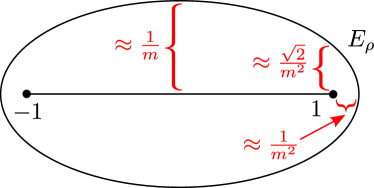
Figure 4: Distances $1-a$, $b$, and the intersection of $x=1$ with the Bernstein ellipse as a function of $m$. The distance from $z=1$ to the intersection of $E_{\rho}$ with the $\operatorname{Re}(\cos\phi)$ axis is $\approx 1/m^{2}$, and is equal to $1-a$, where $a$ is the semi-major axis of $E_{\rho}$. The intersection of $x=1$ with $E_{\rho}$ has a distance of $\approx\sqrt{2}/m^{2}$ to the point $z=1$. The vertical distance from $z=0$ to $E_{\rho}$ is $\approx 1/m$, and is equal to $b$, the semi-minor axis of $E_{\rho}$.

3.4.3 Length of Gustafsson’s Contours within the Bernstein Ellipse

Recall from Section 3.1.1 that Gustafsson’s contours $\gamma_{1}$ and $\gamma_{2}$ can be parameterized as

$$\widetilde{\gamma_{1}}(\tau)=\tau^{4}+2i\beta_{-}\tau^{2}+1,$$ (115)

$$\widetilde{\gamma_{2}}(\tau)=\tau^{4}+2i\beta_{+}\tau^{2}-1.$$ (116)

Consider the sets $\Gamma_{1}$, $\Gamma_{2}$, consisting of all possible $\gamma_{1}$, and $\gamma_{2}$, respectively, defined as

$$\Gamma_{1}=\{\gamma_{1}:0<\beta_{-}<\infty\},\qquad\Gamma_{2}=\{\gamma_{2}:1<\beta_{+}<\infty\}.$$ (117)

The boundary of $\Gamma_{2}$, denoted as $\partial\Gamma_{2}$, is given by $\gamma_{2}$ associated with $\beta_{+}=1$ and the $\gamma_{1}$ associated with $\beta_{+}=\infty$. We observe that in the limit as $\beta_{-}\to\infty$, formula (114) resembles a vertical line (see Figure 5). Together with bounds from Section 3.4.2, it is clear that the angle that $\partial\Gamma_{2}$ makes with $E_{\rho}$ is bounded from below.

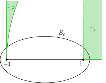
Figure 5: The intersection of all possible Gustafsson contours with the Bernstein ellipse $E_{\rho}$ in the $z=\cos\phi$ plane. Recall that Gustafsson’s contours are denoted $\gamma_{1}$ and $\gamma_{2}$, where $\gamma_{1}$ begins at the point $z=1$ and $\gamma_{2}$ begins at the point $z=-1$. The set of all possible $\gamma_{1}$ is denoted $\Gamma_{1}$. The set of all possible $\gamma_{2}$ is denoted $\Gamma_{2}$.

3.5 Evaluating the Modal Green’s Function

After the variable substitution of $z=\cos\phi$, $dz=-\sin{\phi}\,d\phi$, the formula for the modal Green’s function, $G_{m}$, is

$$G_{m}=\int\displaylimits_{[-1,1]}\frac{e^{-i\kappa\sqrt{1-\alpha z}}}{\sqrt{1-\alpha z}\sqrt{1-z^{2}}}T_{m}(z)dz.$$ (118)

Our rational function approximation, $R_{m}(z)$, is approximately equal to $T_{m}(z)$ on the interval $[-1,1]$. Therefore, substituting $R_{m}(z)$ for $T_{m}(z)$, we arrive at a formula for $G_{m}$,

$$G_{m}\approx\int\displaylimits_{[-1,1]}\frac{e^{-i\kappa\sqrt{1-\alpha z}}}{\sqrt{1-\alpha z}\sqrt{1-z^{2}}}R_{m}(z)dz.$$ (119)

The integrand of (119) is analytic everywhere in the complex plane except for a finite number of poles, so the integral can be deformed. By Cauchy’s residue theorem,

$$\oint_{\Gamma}\frac{e^{-i\kappa\sqrt{1-\alpha z}}}{\sqrt{1-\alpha z}\sqrt{1-z^{2}}}R_{m}(z)dz=2\pi i\sum_{k=1}^{n}\underset{z=z_{k}}{\text{Res}}\Bigg{(}\frac{e^{-i\kappa\sqrt{1-\alpha z}}}{\sqrt{1-\alpha z}\sqrt{1-z^{2}}}R_{m}(z)\Bigg{)},$$ (120)

where $z_{1},...,z_{n}$ are the poles inside $\Gamma$. Thus, if $\Gamma$ is a closed contour containing the interval $[-1,1]$, we have that

$$G_{m}\approx-\int\displaylimits_{\Gamma\setminus[-1,1]}\frac{e^{-i\kappa\sqrt{1-\alpha z}}}{\sqrt{1-\alpha z}\sqrt{1-z^{2}}}R_{m}(z)dz+2\pi i\sum_{k=1}^{n}\underset{z=z_{k}}{\text{Res}}\Bigg{(}\frac{e^{-i\kappa\sqrt{1-\alpha z}}}{\sqrt{1-\alpha z}\sqrt{1-z^{2}}}R_{m}(z)\Bigg{)},$$ (121)

where $\Gamma$ is a contour starting at $z=1$ and ending at $z=-1$. We select $\Gamma\setminus[-1,1]$ to be the Gustafsson contour $\gamma_{1}+\gamma_{c}+\gamma_{2}$, which we described in Section 3.1.1. Since the integrand vanishes over $\gamma_{c}$, we have that

$$\begin{split}G_{m}\approx&\int_{\gamma_{1}}\frac{e^{-i\kappa\sqrt{1-\alpha z}}}{\sqrt{1-\alpha z}\sqrt{1-z^{2}}}R_{m}(z)dz+\int_{\gamma_{2}}\frac{e^{-i\kappa\sqrt{1-\alpha z}}}{\sqrt{1-\alpha z}\sqrt{1-z^{2}}}R_{m}(z)dz\\ &\qquad+2\pi i\sum_{k=1}^{n}\underset{z=z_{k}}{\text{Res}}\Bigg{(}\frac{e^{-i\kappa\sqrt{1-\alpha z}}}{\sqrt{1-\alpha z}\sqrt{1-z^{2}}}R_{m}(z)\Bigg{)}.\end{split}$$ (122)

3.6 Removing the Singularity

Recall that the integral in (81) corresponding to the $\gamma_{1}$ contour has the formula

$$\int_{\gamma_{1}}\frac{e^{-i\kappa\sqrt{1-\alpha z}}}{\sqrt{1-\alpha z}\sqrt{1-z^{2}}}T_{m}(z)dz=\int_{\gamma_{1}}\frac{e^{-i\kappa\sqrt{1-\alpha z}}}{\sqrt{1-\alpha z}\sqrt{1-z}\sqrt{1+z}}T_{m}(z)dz.$$ (123)

Observe that the integrand in (123) has square-root singularities at $z=1$ and $z=-1$. Furthermore, when $\alpha\approx 1$, the product of the terms,

$$\frac{1}{\sqrt{1-\alpha z}\sqrt{1-z}}\approx\frac{1}{1-z},$$ (124)

meaning that the integrand will have a $1/z$-type singularity at $z=1$. By careful reparameterization of the contour $\gamma_{1}$, the singularities in (123) can be removed. The variable substitutions and analysis of the singularities in this section are unchanged when $R_{m}(z)$ is substituted for $T_{m}(z)$. Recall from Section 3.1.1 that the contour $\gamma_{1}$ can be parameterized as

$$\gamma_{1}(t)=\frac{t^{2}}{4(1/\alpha-1)}+1+it,$$ (125)

for $t>0$. For convenience, we introduce the parameter $\beta_{-}$, defined as

$$\beta_{-}=\sqrt{1/\alpha-1},$$ (126)

and we observe that, since $0\leq\alpha<1$, we have $0<\beta_{-}<\infty$. We then follow [11] and perform the substitution $t=2\beta_{-}\tau^{2}$ and reparameterize the contour $\gamma_{1}$ as $\widetilde{\gamma_{1}}$, given by

$$\widetilde{\gamma_{1}}(\tau)=\gamma_{1}(2\beta_{-}\tau^{2})=\tau^{4}+2i\beta_{-}\tau^{2}+1.$$ (127)

Gustafsson showed (see [11], equations (15) and (16)) that, after substituting $z=\widetilde{\gamma_{1}}(\tau)$, $dz=\widetilde{\gamma_{1}}^{\prime}(\tau)d\tau$,

$$dz=4\tau(\tau^{2}+i\beta_{-})d\tau,$$ (128)

$$\sqrt{1-\alpha z}=-i\sqrt{\alpha}(\tau^{2}+i\beta_{-}).$$ (129)

Thus, with the parameterization $z=\widetilde{\gamma_{1}}(\tau)$, formula (123) becomes

$$\frac{-4i}{\sqrt{\alpha}}\,\int_{0}^{\infty}\frac{e^{-i\kappa\sqrt{1-\alpha\widetilde{\gamma_{1}}(\tau)}}}{\sqrt{1-\widetilde{\gamma_{1}}(\tau)}\sqrt{1+\widetilde{\gamma_{1}}(\tau)}}T_{m}(\tau)d\tau,$$ (130)

where we have used (128) and (129) to cancel the $\sqrt{1-\alpha z}$ term. The integrand in (130) has a square-root singularity near $z=1$. Substituting (127) into (130), we have

$$\frac{-4i}{\sqrt{\alpha}}\int\frac{e^{-i\kappa\sqrt{1-\alpha\widetilde{\gamma_{1}}(\tau)}}}{\sqrt{-(\tau^{4}+2i\beta_{-}\tau^{2})}\sqrt{1+\widetilde{\gamma_{1}}(\tau)}}T_{m}(\widetilde{\gamma_{1}}(\tau))\tau d\tau,$$ (131)

which can be simplified to

$$\frac{-4}{\sqrt{\alpha}}\int_{0}^{\infty}\frac{e^{-i\kappa\sqrt{1-\alpha\widetilde{\gamma_{1}}(\tau)}}}{\sqrt{\tau^{2}+2i\beta_{-}}\sqrt{1+\widetilde{\gamma_{1}}(\tau)}}T_{m}(\widetilde{\gamma_{1}}(\tau))d\tau.$$ (132)

Note that the integrand of (132) is the product of a smooth function and the function $1/\sqrt{\tau^{2}+2i\beta_{-}}$. Let $F_{1}(\widetilde{\gamma_{1}}(\tau))$ be the smooth term, given by the formula

$$F_{1}(\tau)=\frac{e^{-i\kappa\sqrt{1-\alpha\widetilde{\gamma_{1}}_{1}(\tau)}}}{\sqrt{1+\widetilde{\gamma_{1}}(\tau)}}T_{m}(\widetilde{\gamma_{1}}(\tau))$$ (133)

We now rewrite (132) using (133), so that

$$\frac{-4}{\sqrt{\alpha}}\int_{0}^{\infty}\frac{F_{1}(\tau)}{\sqrt{\tau^{2}+i\beta_{-}}}d\tau.$$ (134)

The variable substitutions for the integral corresponding to the $\gamma_{2}$ contour are similar. Recall that $\gamma_{2}$ can be parameterized as

$$\gamma_{2}(t)=\frac{t^{2}}{1/\alpha+1}-1+it.$$ (135)

For the $\gamma_{2}$ contour, we introduce the parameter $\beta_{+}$, defined as

$$\beta_{+}=\sqrt{1/\alpha+1},$$ (136)

and we observe that, since $0\leq\alpha<1$, we have $1<\beta_{+}<\infty$. We reparameterize $\gamma_{2}(t)$ as $\widetilde{\gamma_{2}}(t)$, given by the formula

$$\widetilde{\gamma_{2}}(\tau)=\tau^{4}+2i\beta_{+}\tau^{2}-1,$$ (137)

By proceeding as before, we arrive at the formula for $F_{2}(\tau)$,

$$F_{2}(\tau)=\frac{e^{-i\kappa\sqrt{1-\alpha\widetilde{\gamma_{2}}(\tau)}}}{\sqrt{1-\widetilde{\gamma_{2}}(\tau)}}T_{m}(\widetilde{\gamma_{2}}(\tau)).$$ (138)

The formula for the integral corresponding to the $\gamma_{2}$ contour is thus

$$\frac{4i}{\sqrt{\alpha}}\int_{0}^{\infty}\frac{F_{2}(\tau)}{\sqrt{\tau^{2}+2i\beta_{+}}}d\tau.$$ (139)

We combine (134) and (139) to write a formula for the $m$th modal Green’s function,

$$G_{m}=\frac{-4}{\sqrt{\alpha}}\int_{0}^{\infty}\frac{F_{1}(\tau)}{\sqrt{\tau^{2}+2i\beta_{-}}}d\tau+\frac{4i}{\sqrt{\alpha}}\int_{0}^{\infty}\frac{F_{2}(\tau)}{\sqrt{\tau^{2}+2i\beta_{+}}}d\tau.$$ (140)

Because $\beta_{+}$ is bounded from below by $1$, the denominator in (139) is always greater than $1$. In contrast, when $\alpha\approx 1$, we have that $\beta_{-}\approx 0$, which means that the denominator in (134) $\approx\sqrt{\tau^{2}}=\tau$.

3.7 Intersection of the Bernstein Ellipse with the Gustafsson Contour

It is natural to split each contour integral into two segments, one within the Bernstein ellipse and one beyond the ellipse. In this section, we solve for the locations where the Gustafsson contour, $\gamma_{1}\cup\gamma_{2}$ (introduced in 3.1.1), intersects the Bernstein ellipse in the $z=\cos\phi$-plane. We derive formulae in terms of the Bernstein ellipse’s parameter and in terms of the Gustafsson contours’ parameter.

3.7.1 Intersection in Terms of the Bernstein Ellipse’s Parameter

Recall from Section 2.2 that the Bernstein ellipse, $E_{\rho}$, is parameterized by the formula

$$E_{\rho}(\theta)=a\cos\theta+ib\sin\theta,$$ (141)

for $\theta\in[0,2\pi)$, where

$$a=\frac{1}{2}(\rho+\rho^{-1}),\qquad b=\frac{1}{2}(\rho-\rho^{-1}).$$ (142)

Also recall from Section 3.1.1 that Gustfasson’s contours, $\gamma_{1}$ and $\gamma_{2}$, can be reparameterized as

$$\widetilde{\gamma_{1}}(\tau)=\tau^{4}+2i\beta_{-}\tau^{2}+1,$$ (143)

$$\widetilde{\gamma_{2}}(\tau)=\tau^{4}+2i\beta_{+}\tau^{2}-1,$$ (144)

where

$$\beta_{-}=\sqrt{1/\alpha-1},\qquad\beta_{+}=\sqrt{1/\alpha+1}.$$ (145)

To solve for the parameter $\theta$ for which $E_{\rho}(\theta)$ intersects $\widetilde{\gamma}_{1}$, we substitute the real and imaginary parts of $E\rho$ into $\widetilde{\gamma}_{1}$, to arrive at a quadratic equation in theta.

Let $s$ be the larger of the two roots of

$$\frac{b^{2}}{4\beta_{+}^{2}}s^{2}+as+\Big{(}1+\frac{b^{2}}{4\beta_{+}^{2}}\Big{)}=0.$$ (146)

Then,

$$\theta=\arccos(s)$$ (147)

A similar procedure is used to solve for $\tau$ such that of $\widetilde{\gamma}_{2}(\tau)$ intersects $E_{\rho}$, resulting in the formula

$$\frac{b^{2}}{4\beta_{-}^{2}}s^{2}+as+\Big{(}-1+\frac{b^{2}}{4\beta_{-}^{2}}\Big{)}=0.$$ (148)

Then

$$\theta=\arccos(s)$$ (149)

3.7.2 Intersection in Terms of the Gustafsson’s Contours’ Parameters

We now solve for parameter $\tau$ for which $\widetilde{\gamma}_{1}(\tau)$ intersects $E_{\rho}$.

Let $s>0$ be the positive root of

$$s^{2}+\Big{(}\frac{4a^{2}\beta_{-}^{2}}{b^{2}}+2\Big{)}s+(1-a^{2})=0.$$ (150)

Then,

$$\tau=s^{\frac{1}{4}}.$$ (151)

The parameter $\tau$ for which $\widetilde{\gamma}_{2}(\tau)$ intersects $E_{\rho}$ is solved in a similar fashion.

$$s^{2}+\Big{(}\frac{4a^{2}\beta_{+}^{2}}{b^{2}}-2\Big{)}s+(1-a^{2})=0.$$ (152)

Then,

$$\tau=s^{\frac{1}{4}}.$$ (153)

4 Algorithm

Recall that the method of Epstein et al. [9] has computational cost which scales with both $|\kappa|$ and $1/(1-\alpha)$, and cannot be easily parallelized (see Section 1.2.2). In contrast, the method of Gustafsson [11] has computational cost independent of $\kappa$ and $\alpha$, but incurs cancellation error which grows geometrically in $m$ (see Section 3.1.2).

Our technique is to compute the modal Green’s function by integrating along Gustafsson’s contours using a rational function approximation in place of the Chebyshev polynomial. Because the spherical wave term in the integrand monotonically decays, our algorithm’s order is completely independent of $\kappa$. Unlike the method of Gustafsson, because our rational function approximation $R_{m}(z)$ is bounded by our choice of Bernstein ellipse $\rho$, our approach does not have cancellation error which geometrically grows in $m$. This comes at the price of having to evaluate the residues of $R_{m}$ on the boundary of the corresponding Bernstein ellipse $E_{\rho}$, which scales with $m$. We also use the same technique as Gustafsson to evaluate the Green’s function when $\alpha\approx 1$, in time independent of of $\alpha$. Consequently, our algorithm’s computational cost depends only on $m$ and is independent of both $\kappa$ and $\alpha$, and scales as $O(m)$.

4.1 Choice of the Rational Function Approximation

Recall from Section 3.2.3 that the Chebyshev polynomial $T_{m}(z)$ can be approximated on the interval $[-1,1]$ with a rational function, $R_{m}(z)$, constructed via an application of Cauchy’s integral formula followed by the application of a quadrature rule. This rational function approximation decays quickly in the complex plane. In this section, we introduce a different approximation, also denoted $R_{m}(z)$, which is the sum of a Cauchy integral and a rational function.

By Cauchy’s integral formula, $T_{m}(z)$ can be expressed as the contour integral,

$$T_{m}(z)=\frac{1}{2\pi i}\oint\limits_{\Gamma}\frac{T_{m}(v)}{v-z}dv,$$ (154)

where $\Gamma$ is any simple closed contour, and $z$ is a point in the interior of $\Gamma$. Similarly,

$$\frac{1}{2\pi i}\oint_{\Gamma}\frac{T_{m}(v)}{v-z}dv=0,$$ (155)

for all $z$ outside $\Gamma$. Recall from 3.2.2 that for any $m$th order Chebyshev polynomial, there is an associated $\rho$ such that, within the Bernstein ellipse $E_{\rho}$, $T_{m}(z)$ is bounded by the constant $M$. Furthermore, within the interior of $E_{\rho}$, the Chebyshev polynomial oscillates exactly once along any possible Gustafsson contour (see Section 3.4). Note that the parameter $\rho$ associated with the Bernstein ellipse $E_{\rho}$ is a function of $m$, but we denote it simply as $\rho$. We also denote a scaled copy of $E_{\rho}$ by $E_{\widetilde{\rho}}$, where $E_{\widetilde{\rho}}$ has twice the major axis and twice the minor axis of $E_{\rho}$ (see Figure 6). Note that $E_{\widetilde{\rho}}$ is not a Bernstein ellipse.

Let $C_{\rho}$ denote the part of the Bernstein ellipse $E_{\rho}$ between the contours $\gamma_{1}$ and $\gamma_{2}$, represented as the blue arc between $p_{1}$ and $p_{2}$ in Figure 6, where $p_{1}\in\mathbb{C}$ and $p_{2}\in\mathbb{C}$ are the intersection points of $\gamma_{1}$ and $\gamma_{2}$ with $E_{\rho}$, respectively. We split the Cauchy integral into two parts,

$$T_{m}(z)=\frac{1}{2\pi i}\int\displaylimits_{C_{\rho}}\frac{T_{m}(v)}{v-z}dv+\frac{1}{2\pi i}\int\displaylimits_{E\rho\setminus C_{\rho}}\frac{T_{m}(v)}{v-z}dv$$ (156)

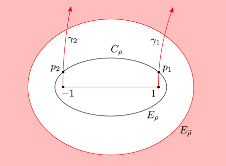
Figure 6: Contours of interest with respect to the function $R_{m}(z)$ in the $z=\cos\phi$ plane. Gustafsson’s contours are labeled as $\gamma_{1}$ and $\gamma_{2}$. The inner Bernstein ellipse is denoted by $E_{\rho}$. The outer ellipse is denoted by $E_{\widetilde{\rho}}$. The intersection of $\gamma_{1}$ with $E_{\rho}$ is denoted by $p_{1}$, and the intersection of $\gamma_{2}$ with $E_{\rho}$ is denoted by $p_{2}$. The arc of $E_{\rho}$ between $p_{2}$ and $p_{1}$ is denoted by $C_{\rho}$. The contours highlighted in red and region shaded in red correspond to the values of $z$ on which the quadrature in (157) must be accurate, in the sense of (159)-(162).

Now, suppose that $\theta_{1},\ldots,\theta_{n}$, $w_{1},\ldots,w_{n}$ are the nodes and weights of a quadrature formula such that

$$\frac{1}{2\pi i}\int\limits_{C_{\rho}}\frac{T_{m}(v)}{v-z}dv\approx\frac{1}{2\pi i}\sum_{i=1}^{n}\frac{T_{m}(v_{i})}{v_{i}-z}dv_{i}w_{i},$$ (157)

where $v_{i}=E_{\rho}(\theta_{i})$, $dv_{i}=E_{\rho}^{\prime}(\theta_{i})$, and the quadrature is accurate to precision $\epsilon>0$ for all $z\in[-1,1]$, $z\in\gamma_{1}\cap E_{\widetilde{\rho}}^{o}$, $z\in\gamma_{2}\cap E_{\widetilde{\rho}}^{o}$, $z\in\mathbb{C}\setminus E_{\widetilde{\rho}}^{o}$, where $E_{\widetilde{\rho}}^{o}$ is the interior of $E_{\widetilde{\rho}}$ (see Figure 6). Now, let $R_{m}(z)$ be defined by

$$R_{m}(z)=\frac{1}{2\pi i}\int\displaylimits_{E\rho\setminus C_{\rho}}\frac{T_{m}(v)}{v-z}dv+\frac{1}{2\pi i}\sum_{i=1}^{N}\frac{T_{m}(v_{i})}{v_{i}-z}dv_{i}w_{i}.$$ (158)

We observe that, due to formula (154), we have that

$$|T_{m}(z)-R_{m}(z)|<\epsilon,$$ (159)

for $z\in[-1,1]$. We also observe that, due to formula (154), we have that

$$|T_{m}(z)-R_{m}(z)|<\epsilon,$$ (160)

for $z\in\gamma_{1}\cap E_{\rho}^{o}$ and $z\in\gamma_{2}\cap E_{\rho}^{o}$. Likewise, due to formula (155),

$$|R_{m}(z)|<\epsilon,$$ (161)

for $z\in\gamma_{1}\setminus E_{\rho}^{o}$ and $z\in\gamma_{2}\setminus E_{\rho}^{o}$. We also observe that, due to formula (155),

$$|R_{m}(z)|<\epsilon,$$ (162)

for $z\in\mathbb{C}\setminus E_{\widetilde{\rho}}^{o}$.

4.1.1 Deformation of the Contour

Recall from Section 3.5 that after the variable substitution of $z=\cos\phi$, $dz=-\sin{\phi}\,d\phi$, the formula for the modal Green’s function, $G_{m}$, is

$$G_{m}=\int\displaylimits_{[-1,1]}\frac{e^{-i\kappa\sqrt{1-\alpha z}}}{\sqrt{1-\alpha z}\sqrt{1-z^{2}}}T_{m}(z)dz.$$ (163)

Our approximation, $R_{m}(z)$, by formula (154), is approximately equal to $T_{m}(z)$ on the interval $[-1,1]$. Therefore, substituting $R_{m}(z)$ for $T_{m}(z)$, we arrive at a formula for $G_{m}$,

$$G_{m}\approx\int\displaylimits_{[-1,1]}\frac{e^{-i\kappa\sqrt{1-\alpha z}}}{\sqrt{1-\alpha z}\sqrt{1-z^{2}}}R_{m}(z)dz.$$ (164)

The integrand of (164) is analytic everywhere in the complex plane except for a finite number of poles, so the integral can be deformed. Recall that, for any closed contour $\Gamma\in\mathbb{C}$, by Cauchy’s residue theorem,

$$\oint_{\Gamma}\frac{e^{-i\kappa\sqrt{1-\alpha z}}}{\sqrt{1-\alpha z}\sqrt{1-z^{2}}}R_{m}(z)dz=2\pi i\sum_{k=1}^{n}\underset{z=z_{k}}{\text{Res}}\Bigg{(}\frac{e^{-i\kappa\sqrt{1-\alpha z}}}{\sqrt{1-\alpha z}\sqrt{1-z^{2}}}R_{m}(z)\Bigg{)},$$ (165)

where $z_{1},...,z_{n}$ are the poles inside $\Gamma$. For brevity, let the portion of the integrand in (165) corresponding to the spherical wave component be represented by the function $H(z)$, given by

$$H(z)=\frac{e^{-i\kappa\sqrt{1-\alpha z}}}{\sqrt{1-\alpha z}\sqrt{1-z^{2}}}.$$ (166)

If $\Gamma$ is a closed contour containing the interval $[-1,1]$, we have that

$$G_{m}\approx-\int\displaylimits_{\Gamma\setminus[-1,1]}H(z)R_{m}(z)dz+2\pi i\sum_{k=1}^{n}\underset{z=z_{k}}{\text{Res}}\bigg{(}H(z)R_{m}(z)\bigg{)},$$ (167)

where we have substituted formula (166) for the spherical wave term. We select $\Gamma\setminus[-1,1]$ to be Gustafsson’s contours within the outer ellipse, $E_{\widetilde{\rho}}$, with both segments connected by a short segment $\gamma_{c}\subset\mathbb{C}\setminus E_{\widetilde{\rho}}^{o}$ (see Figure 7).

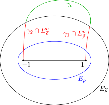
Figure 7: Contours used in formula (168) in the $z=\cos\phi$ plane. The interior Bernstein ellipse is denoted by $E_{\rho}$ and drawn in blue. The exterior ellipse is denoted by $E_{\widetilde{\rho}}$. Gustafsson’s contours within the exterior ellipse are denoted by $\gamma_{2}\cap E_{\widetilde{\rho}}^{o}$ and $\gamma_{2}\cap E_{\widetilde{\rho}}^{o}$ and drawn in red. The contour $\gamma_{c}\subset\mathbb{C}\setminus E_{\widetilde{\rho}}^{o}$, connecting the $\gamma_{1}$ and $\gamma_{2}$ segments, is drawn in green. The intersection of $\gamma_{1}$ with $E_{\rho}$ is denoted by $p_{1}$, and the intersection of $\gamma_{2}$ with $E_{\rho}$ is denoted by $p_{2}$.

Substituting this choice of $\Gamma\setminus[-1,1]$ into (167), we have

$$\begin{split}G_{m}\approx\int\displaylimits_{\gamma_{1}\cap E_{\widetilde{\rho}}^{o}}H(z)R_{m}(z)dz+\int\displaylimits_{\gamma_{2}\cap E_{\widetilde{\rho}}^{o}}H(z)R_{m}(z)dz+\int\displaylimits_{\gamma_{c}}H(z)R_{m}(z)dz\\ +2\pi i\sum_{k=1}^{n}\underset{z=z_{k}}{\text{Res}}\Bigg{(}H(z)R_{m}(z)\Bigg{)},\end{split}$$ (168)

where $\gamma_{1}$ and $\gamma_{2}$ are Gustafsson’s contours as described in Section 3.1.1, and $E_{\widetilde{\rho}}^{o}$ is the interior of the scaled Bernstein ellipse introduced earlier (see Figure 7). We split the integral corresponding to the $\gamma_{1}$ contour into

$$\int\displaylimits_{\gamma_{1}}H(z)R_{m}(z)dz=\int\displaylimits_{\gamma_{1}\cap E_{\rho}^{o}}H(z)R_{m}(z)dz+\int\displaylimits_{\gamma_{1}\setminus E_{\rho}^{o}}H(z)R_{m}(z)dz.$$ (169)

Recall that by formula (160), $R_{m}(z)\approx T_{m}(z)$ for $z\in\gamma_{1}\cap E_{\rho}^{o}$ and for $z\in\gamma_{2}\cap E_{\rho}^{o}$. Also, recall that by formula (161), $R_{m}(z)\approx\epsilon$ for $z\in\gamma_{1}\setminus E_{\rho}^{o}$ and for $z\in\gamma_{2}\setminus E_{\rho}^{o}$. Substituting (160) and (161) into (169), we arrive at a formula for the $\gamma_{1}$ contour within the interior of $E_{\widetilde{\rho}}$,

$$\int\displaylimits_{\gamma_{1}\cap E_{\widetilde{\rho}}^{o}}H(z)R_{m}(z)dz\approx\int\displaylimits_{\gamma_{1}\cap E_{\rho}^{o}}H(z)T_{m}(z)dz.$$ (170)

Likewise, the formula for the $\gamma_{2}$ contour within the interior of $E_{\widetilde{\rho}}$ is

$$\int\displaylimits_{\gamma_{2}\cap E_{\widetilde{\rho}}^{o}}H(z)R_{m}(z)dz\approx\int\displaylimits_{\gamma_{2}\cap E_{\rho}^{o}}H(z)T_{m}(z)dz.$$ (171)

We also observe that, due to formula (162), the integral corresponding to $\gamma_{c}$ evaluates to zero. We now substitute our formulas for the $\gamma_{1}\cap E_{\widetilde{\rho}}^{o}$, $\gamma_{2}\cap E_{\widetilde{\rho}}^{o}$, and $\gamma_{c}$ contours into (168) to arrive at

$$\begin{split}G_{m}\approx\int\displaylimits_{\gamma_{1}\cap E_{\rho}^{o}}\frac{e^{-i\kappa\sqrt{1-\alpha z}}}{\sqrt{1-\alpha z}\sqrt{1-z^{2}}}T_{m}(z)dz+\int\displaylimits_{\gamma_{2}\cap E_{\rho}^{o}}\frac{e^{-i\kappa\sqrt{1-\alpha z}}}{\sqrt{1-\alpha z}\sqrt{1-z^{2}}}T_{m}(z)dz\\ +2\pi i\sum_{k=1}^{n}\underset{z=z_{k}}{\text{Res}}\Bigg{(}\frac{e^{-i\kappa\sqrt{1-\alpha z}}}{\sqrt{1-\alpha z}\sqrt{1-z^{2}}}R_{m}(z)\Bigg{)}.\end{split}$$ (172)

4.1.2 Interpretation of the Residues in Formula (172) as a Quadrature Formula for the Contour $C_{\rho}$

By Cauchy’s integral theorem,

$$G_{m}\approx\int\displaylimits_{\gamma_{1}\cap E_{\rho}^{o}}H(z)T_{m}(z)dz+\int\displaylimits_{\gamma_{2}\cap E_{\rho}^{o}}H(z)T_{m}(z)dz+\int\displaylimits_{C_{\rho}}H(z)T_{m}(z)dz,$$ (173)

where $\gamma_{1}$, $\gamma_{2}$, $E_{\rho}^{o}$, and $C_{\rho}$ are described in Section 4.1.

Subtracting (172) from (173), and rearranging, we arrive at a formula for the $C_{\rho}$ contour,

$$\int\displaylimits_{C_{\rho}}\frac{e^{-i\kappa\sqrt{1-\alpha z}}}{\sqrt{1-\alpha z}\sqrt{1-z^{2}}}T_{m}(z)dz\approx 2\pi i\sum_{k=1}^{n}\underset{z=z_{k}}{\text{Res}}\Bigg{(}\frac{e^{-i\kappa\sqrt{1-\alpha z}}}{\sqrt{1-\alpha z}\sqrt{1-z^{2}}}R_{m}(z)\Bigg{)}.$$ (174)

Recall from Section 4.1 that

$$R_{m}(z)=\frac{1}{2\pi i}\int\displaylimits_{E\rho\setminus C_{\rho}}\frac{T_{m}(v)}{v-z}dv+\frac{1}{2\pi i}\sum_{i=1}^{n}\frac{T_{m}(v_{i})}{v_{i}-z}dv_{i}w_{i},$$ (175)

where $v_{i}=E_{\rho}(\theta_{i})$, $dv_{i}=E_{\rho}^{\prime}(\theta_{i})$, and $\theta_{1},\ldots,\theta_{n}$, $w_{1},\ldots,w_{n}$ are nodes and weights of the quadrature constructed in (157). Thus, the residues $z_{1},\ldots,z_{n}$ in (174) correspond to the points $v_{1},\ldots,v_{n}$ and

$$2\pi i\sum_{i=1}^{n}\underset{z=z_{i}}{\text{Res}}\Bigg{(}\frac{e^{-i\kappa\sqrt{1-\alpha z}}}{\sqrt{1-\alpha z}\sqrt{1-z^{2}}}R_{m}(z)\Bigg{)}=\sum_{i=1}^{n}\frac{e^{-i\kappa\sqrt{1-\alpha v_{i}}}}{\sqrt{1-\alpha v_{i}}\sqrt{1-v_{i}^{2}}}T_{m}(v_{i})dv_{i}w_{i}.$$ (176)

Substituting (176) into (174), we have that

$$\sum_{i=1}^{n}\frac{e^{-i\kappa\sqrt{1-\alpha v_{i}}}}{\sqrt{1-\alpha v_{i}}\sqrt{1-v_{i}^{2}}}T_{m}(v_{i})dv_{i}w_{i}\approx\int\displaylimits_{C_{\rho}}\frac{e^{-i\kappa\sqrt{1-\alpha z}}}{\sqrt{1-\alpha z}\sqrt{1-z^{2}}}T_{m}(z)dz,$$ (177)

which resembles a quadrature formula for the contour integral on $C_{\rho}$. Substituting formula (177) into formula (172), we arrive at

$$\begin{split}G_{m}\approx\int\displaylimits_{\gamma_{1}\cap E_{\rho}^{o}}\frac{e^{-i\kappa\sqrt{1-\alpha z}}}{\sqrt{1-\alpha z}\sqrt{1-z^{2}}}T_{m}(z)dz+\int\displaylimits_{\gamma_{2}\cap E_{\rho}^{o}}\frac{e^{-i\kappa\sqrt{1-\alpha z}}}{\sqrt{1-\alpha z}\sqrt{1-z^{2}}}T_{m}(z)dz\\ +\sum_{i=1}^{n}\frac{e^{-i\kappa\sqrt{1-\alpha v_{i}}}}{\sqrt{1-\alpha v_{i}}\sqrt{1-v_{i}^{2}}}T_{m}(v_{i})dv_{i}w_{i},\end{split}$$ (178)

where $v_{i}=E_{\rho}(\theta_{i})$, $dv_{i}=E_{\rho}^{\prime}(\theta_{i})$, and $\theta_{1},\ldots,\theta_{n}$, $w_{1},\ldots,w_{n}$ are the nodes and weights of the quadrature constructed in (157).

4.2 Evaluation of the Integral on Gustafsson’s Contour when $\alpha\approx 1$

Recall from Section 4.1.2 that the formula for the $m$th modal Green’s function is

$$\begin{split}G_{m}\approx\int\displaylimits_{\gamma_{1}\cap E_{\rho}^{o}}\frac{e^{-i\kappa\sqrt{1-\alpha z}}}{\sqrt{1-\alpha z}\sqrt{1-z^{2}}}T_{m}(z)dz+\int\displaylimits_{\gamma_{2}\cap E_{\rho}^{o}}\frac{e^{-i\kappa\sqrt{1-\alpha z}}}{\sqrt{1-\alpha z}\sqrt{1-z^{2}}}T_{m}(z)dz\\ +\sum_{i=1}^{n}\frac{e^{-i\kappa\sqrt{1-\alpha v_{i}}}}{\sqrt{1-\alpha v_{i}}\sqrt{1-v_{i}^{2}}}T_{m}(v_{i})dv_{i}w_{i},\end{split}$$ (179)

where $v_{i}=E_{\rho}(\theta_{i})$, $dv_{i}=E_{\rho}^{\prime}(\theta_{i})$, and $\theta_{1},\ldots,\theta_{n}$, $w_{1},\ldots,w_{n}$ are the nodes and weights of the quadrature constructed in (157). Recall also from Section 3.6 that the integrals in (179) can be written as

$$\begin{split}G_{m}\approx\frac{-4}{\sqrt{\alpha}}\int_{0}^{\tau_{1}}\frac{F_{1}(\tau)}{\sqrt{\tau^{2}+2i\beta_{-}}}d\tau+\frac{4}{\sqrt{\alpha}}\int_{0}^{\tau_{2}}\frac{F_{2}(\tau)}{\sqrt{\tau^{2}+2i\beta_{+}}}d\tau\\ +\sum_{i=1}^{n}\frac{e^{-i\kappa\sqrt{1-\alpha v_{i}}}}{\sqrt{1-\alpha v_{i}}\sqrt{1-v_{i}^{2}}}T_{m}(v_{i})dv_{i}w_{i},\end{split}$$ (180)

where $F_{1}(\tau)$ and $F_{2}(\tau)$ are smooth functions corresponding to the $\gamma_{1}$ and $\gamma_{2}$ contours, respectively (see Section 3.6, equations (134) and (139)), $\tau_{1}$ and $\tau_{2}$ are positive parameters such that $\gamma_{1}(\tau_{1})$ and $\gamma_{2}(\tau_{2})$ intersect $E_{\rho}$, respectively, and

$$\beta_{-}=\sqrt{1/\alpha-1},\qquad\beta_{+}=\sqrt{1/\alpha+1}.$$ (181)

When $\alpha\approx 1$, the parameter $\beta_{+}\approx 2$, meaning that the integrand in (180) corresponding $\gamma_{2}$ remains a smooth function of $\tau$ for all values of $0\leq\alpha<1$, and can be evaluated efficiently with a Gauss-Legendre quadrature. In contrast, when $\alpha\approx 1$, the parameter $\beta_{-}\approx 0$. Consequently, for $\alpha\approx 1$, the integrand in (180) corresponding to the $\gamma_{1}$ contour resembles a $1/\tau$ singularity at $\tau=0$.

4.2.1 Evaluation of the Integral on the Contour $\gamma_{1}$ when $\alpha\approx 1$

We integrate along the contour $\gamma_{1}$ using the following procedure. Observe that for $\tau$ sufficiently large, the integrand is smooth. Thus we split the integral into two parts,

$$\frac{-4}{\sqrt{\alpha}}\int_{0}^{\tau_{1}}\frac{F_{1}(\tau)}{\sqrt{\tau^{2}+i\beta_{-}}}d\tau=\frac{-4}{\sqrt{\alpha}}\int_{0}^{\tau_{0}}\frac{F_{1}(\tau)}{\sqrt{\tau^{2}+i\beta_{-}}}d\tau+\frac{-4}{\sqrt{\alpha}}\int_{\tau_{0}}^{\tau_{1}}\frac{F_{1}(\tau)}{\sqrt{\tau^{2}+i\beta_{-}}}d\tau.$$ (182)

The integral corresponding to the interval $[\tau_{0},\tau_{1}]$ can be efficiently computed using a Gauss-Legendre quadrature. The integral corresponding to the interval $[0,\tau_{0}]$ is evaluated with a specialized quadrature based on the technique used by Gustafsson (see [11], Section 4.2), described below. Recall that $F_{1}(\tau)$ is smooth, given by the formula

$$F_{1}(\tau)=\frac{e^{-i\kappa\sqrt{1-\alpha\widetilde{\gamma_{1}}(\tau)}}}{\sqrt{1+\widetilde{\gamma_{1}}(\tau)}}T_{m}(\widetilde{\gamma_{1}}(\tau)),$$ (183)

where $\widetilde{\gamma_{1}}(\tau)$ is

$$\widetilde{\gamma_{1}}(\tau)=\tau^{4}+i\beta_{-}\tau^{2}+1.$$ (184)

We expand $F_{1}(\tau)$ in k terms of its Taylor series about the point $\tau=0$, given by the formula

$$F_{1}(\tau)\approx\sum_{n=0}^{k}a_{n}\tau^{n}.$$ (185)

We compute the coefficients $a_{n}$ by first forming a Chebyshev expansion of $F_{1}(\tau)$ on the interval $[0,\tau_{0}]$, and then using the mapping (56) described in Section 2.4. This mapping takes the Chebyshev expansion coefficients and returns the corresponding Taylor expansion at $\tau=0$.

We substitute (185) into the integral corresponding to the interal $[0,\tau_{0}]$ from (180), resulting in

$$\frac{-4}{\sqrt{\alpha}}\int_{0}^{\tau_{0}}\frac{F_{1}(\tau)}{\sqrt{\tau^{2}+2i\beta_{-}}}d\tau \approx\frac{-4}{\sqrt{\alpha}}\int_{0}^{\tau_{0}}\frac{\sum_{n=0}^{k}a_{n}\tau^{n}}{\sqrt{\tau^{2}+i\beta_{-}}}d\tau$$ (186)

$$=\frac{-4}{\sqrt{\alpha}}\sum_{n=0}^{k}a_{n}\int_{0}^{\tau_{0}}\frac{\tau^{n}}{\sqrt{\tau^{2}+2i\beta_{-}}}d\tau$$ (187)

Recall from Section 2.3 that the integral of $\tau^{n}$ divided by $\sqrt{a\tau^{2}+b}$ has the recurrence relation

$$\int\frac{\tau^{n}}{\sqrt{a\tau^{2}+b}}d\tau=\frac{\tau^{n-1}\sqrt{a\tau^{2}+b}}{na}-\frac{(n-1)^{b}}{na}\int\frac{\tau^{n-2}}{\sqrt{a\tau^{2}+b}}d\tau,$$ (188)

for $n\geq 2$, where the base case has the formula

$$\int\frac{1}{\sqrt{a\tau^{2}+b}}d\tau=\frac{1}{\sqrt{a}}\ln\Big{(}\tau\sqrt{a}+\sqrt{a\tau^{2}+b}\Big{)},$$ (189)

and this recurrence is known to be stable when $|b|<|a|$. We observe that $\beta_{-}\ll 1$ when $\alpha\approx 1$, meaning that the recurrence given by (188) is stable when applied to (186).

4.3 Construction of the Quadratures to Evaluate the Integral over the Contour $C_{\rho}$

Recall from Section 4.1 that our approximation, $R_{m}(z)$, of the $m$th order Chebyshev polynomial, $T_{m}(z)$, has the formula

$$R_{m}(z)=\frac{1}{2\pi i}\int\displaylimits_{E\rho\setminus C_{\rho}}\frac{T_{m}(v)}{v-z}dv+\frac{1}{2\pi i}\sum_{i=1}^{n}\frac{T_{m}(v_{i})}{v_{i}-z}dv_{i}w_{i},$$ (190)

where $v_{i}=E_{\rho}(\theta_{i})$, $dv_{i}=E_{\rho}^{\prime}(\theta_{i})$, $C_{\rho}$ is the region of the Bernstein ellipse $E_{\rho}$ between and the contours $\gamma_{1}$ and $\gamma_{2}$, and $\theta_{1},\ldots,\theta_{n}$ and $w_{1},\ldots,w_{n}$ are the nodes and weights of a quadrature such that

$$\frac{1}{2\pi i}\int\limits_{C_{\rho}}\frac{T_{m}(v)}{v-z}dv\approx\frac{1}{2\pi i}\sum_{i=1}^{n}\frac{T_{m}(v_{i})}{v_{i}-z}dv_{i}w_{i},$$ (191)

for $z\in[-1,1]$, $z\in\gamma_{1}\cap E_{\widetilde{\rho}}^{o}$, $z\in\gamma_{2}\cap E_{\widetilde{\rho}}^{o}$, $z\in\mathbb{C}\setminus E_{\widetilde{\rho}}^{o}$, where $E_{\widetilde{\rho}}^{o}$ is the interior of $E_{\widetilde{\rho}}$. Recall also from Section 4.1 that, by Cauchy’s integral formula,

$$T_{m}(z)=\oint_{E_{\rho}}\frac{T_{m}(v)}{v-z}dv,$$ (192)

for $z\in E_{\rho}$, where $E_{\rho}$ is the Bernstein ellipse described in Section 4.1. Finally, recall from Section 3.2.2 that, if $\rho=M^{1/m}$, then ${\lvert T_{m}(z)\rvert}<M$ for all $z\in E_{\rho}^{o}$. For the sake of simplicity, we first assume that $M=e$, and then consider the case for general $M$ in Sections 4.3.3 and 4.3.4.

We summarize the contours on which $R_{m}(z)$ approximates $T_{m}(z)$ point-wise by stating that

$$\Big{|}\int_{C_{\rho}}\frac{T_{m}(v)}{v-z}dv-\sum_{i=1}^{n}\frac{T_{m}(v_{i})dv_{i}w_{i}}{v_{i}-z}\Big{|}<\epsilon,$$ (193)

for all $z\in[-1,1]$, $z\in\gamma_{1}\cap E_{\widetilde{\rho}}^{o}$, $z\in\gamma_{2}\cap E_{\widetilde{\rho}}^{o}$, $z\in\mathbb{C}\setminus E_{\widetilde{\rho}}^{o}$, where $E_{\widetilde{\rho}}^{o}$ is the interior of $E_{\widetilde{\rho}}$. Let $p_{1}\in\mathbb{C}$ and $p_{2}\in\mathbb{C}$ denote the intersections of $\gamma_{1}$ and $\gamma_{2}$ with $E_{\rho}$, respectively (see Figure 8).

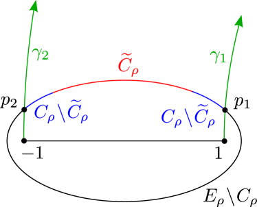
Figure 8: Splitting of the Bernstein ellipse into $\widetilde{C}_{\rho}$ and $C_{\rho}\setminus\widetilde{C}_{\rho}$ based on proximity to Gustafsson’s contours in the $\cos\phi$ plane. Gustafsson’s contours are denoted as $\gamma_{1}$ and $\gamma_{2}$, and drawn in green. The points where $\gamma_{1}$ and $\gamma_{2}$ intersect $E_{\rho}$ are denoted as $p_{1}$ and $p_{2}$, respectively. The region of the ellipse bounded by the intersections $p_{1}$ and $p_{2}$ defines the segment $C_{\rho}$. The segment of $C_{\rho}$ not close to the points $p_{1}$ and $p_{2}$ is denoted as $\widetilde{C}_{\rho}$ and drawn in red. The segments of $C_{\rho}$ which are close to the points $p_{1}$ and $p_{2}$ are denoted as $C_{\rho}\setminus\widetilde{C}_{\rho}$ and drawn in blue. The remainder of the ellipse is denoted as $E_{\rho}\setminus C_{\rho}$ and drawn in black.

Let $\widetilde{C}_{\rho}\subset C_{\rho}$ denote the portion of $C_{\rho}$ no closer than $1/m^{2}$ from the points $p_{1}$ and $p_{2}$, defined by

$$\widetilde{C}_{\rho}=\{z:z\in C_{\rho},|p_{1}-z|>1/m^{2},|p_{2}-z|>1/m^{2}\}.$$ (194)

We split the integral in (157) into $\widetilde{C}_{\rho}$ and $C_{\rho}$, arriving at

$$\int_{C_{\rho}}\frac{T_{m}(v)}{v-z}dv=\int_{\widetilde{C}_{\rho}}\frac{T_{m}(v)}{v-z}dv+\int_{C_{\rho}\setminus\widetilde{C}_{\rho}}\frac{T_{m}(v)}{v-z}dv.$$ (195)

The domain of integration $\widetilde{C}_{\rho}$ is relatively well-separated for all values of $z$ on which the quadrature rule in (193) must hold. In contrast, the domain of integration $C_{\rho}\setminus\widetilde{C}_{\rho}$ is not well-separated. Hence, we split the task of constructing the quadratures on $C_{\rho}$ into two tasks.

4.3.1 Quadratures for the Portion of $C_{\rho}$ Away From Gustafsson’s Contours

Recall from formula (194) that, by construction, $\widetilde{C}_{\rho}$ is separated from the poles near its end points by $1/m^{2}$. Recall also from Section 3.4 that, in the middle, $C_{\rho}$ is separated from the interval $[-1,1]$ by $\approx 1/m$. Hence, by Remark 3.1,

$$\int_{\widetilde{C}_{\rho}}\frac{T_{m}(v)}{v-z}dv$$ (196)

is well approximated by an $O(m)$ Gauss-Legendre quadrature, for all $z\in[-1,1]$, $z\in\gamma_{1}\cap E_{\widetilde{\rho}}^{o}$, $z\in\gamma_{2}\cap E_{\widetilde{\rho}}^{o}$, $z\in\mathbb{C}\setminus E_{\widetilde{\rho}}^{o}$, where $E_{\widetilde{\rho}}^{o}$ is the interior of $E_{\widetilde{\rho}}$.

4.3.2 Quadratures for the Portions of $C_{\rho}$ Near Gustafsson’s Contours

In this section, we present the construction of a quadrature rule which approximates the contour integral

$$\int_{C_{\rho}\setminus\widetilde{C}_{\rho}}\frac{T_{m}(v)}{v-z}dv,$$ (197)

for $z\in[-1,1]$, $z\in\gamma_{1}\cap E_{\widetilde{\rho}}^{o}$, $z\in\gamma_{2}\cap E_{\widetilde{\rho}}^{o}$, $z\in\mathbb{C}\setminus E_{\widetilde{\rho}}^{o}$, where $E_{\widetilde{\rho}}^{o}$ is the interior of $E_{\widetilde{\rho}}$. Since $[-1,1]$ is well-separated from $C_{\rho}\setminus\widetilde{C}_{\rho}$, we focus only on $z\in(\gamma_{1}\cap E_{\widetilde{\rho}})\cup(\gamma_{2}\cap E_{\widetilde{\rho}})$. Observe that $C_{\rho}\setminus\widetilde{C}_{\rho}$ consists of two disjoint segments (see Figure 8). One segment of $C_{\rho}\setminus\widetilde{C}_{\rho}$ approaches the point $p_{1}$, which denotes the intersection of $\gamma_{1}$ (associated with $z=1$) with $E_{\rho}$, the other segment of $C_{\rho}\setminus\widetilde{C}_{\rho}$ approaches the point $p_{2}$, which denotes the intersection of $\gamma_{2}$ (associated with $z=-1$) with $E_{\rho}$. We denote the points where $C_{\rho}\setminus\widetilde{C}_{\rho}$ ends and $\widetilde{C}_{\rho}$ begins with the points $\widetilde{p}_{1}$ and $\widetilde{p}_{2}$, where $\widetilde{p}_{1}$ is the point closer to $p_{1}$, and $\widetilde{p}_{2}$ is the point closer to $p_{2}$. We analyze the segment of $C_{\rho}\setminus\widetilde{C}_{\rho}$ near $p_{2}$, with the understanding that the Bernstein ellipse is symmetric and an identical argument applies to the segment of $C_{\rho}\setminus\widetilde{C}_{\rho}$ near $p_{1}$.

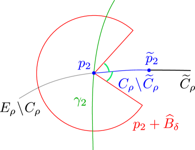
Figure 9: Region $p_{2}+\widehat{B}_{\delta}$ in which the quadrature in formula (191) must accurately evaluate the integral over the contour $C_{\rho}\setminus\widetilde{C}_{\rho}$ for $z\in\gamma_{2}$. The values of $z$ for which the quadrature must be accurate in the sense of formula (205) are the interior of the region denoted by $p_{2}+\widehat{B}_{\delta}$, whose boundary is drawn in red. Note that the angle that $\widehat{B}_{d}$ makes with $C\rho\setminus\widetilde{C}_{\rho}$ is $\pi/6$ from above and $\pi/6$ from below. Gustafsson’s contour which begins at $z=-1$ is denoted $\gamma_{2}$ and is drawn in green. The intersection of $\gamma_{2}$ with the Bernstein Ellipse is denoted by $p_{2}$. The Bernstein ellipse, $E_{\rho}$, is drawn as three contiguous segments. The left segment, colored grey, corresponds to the Bernstein ellipse which is not in $C_{\rho}$, and is denoted $E_{\rho}\setminus C_{\rho}$. The middle segment, denoted $C_{\rho}\setminus\widetilde{C}_{\rho}$, is drawn in blue. The right segment, colored black, corresponds to $\widetilde{C}_{\rho}$. The point where $C_{\rho}\setminus\widetilde{C}_{\rho}$ ends and where $\widetilde{C}_{\rho}$ begins is denoted by $\widetilde{p_{2}}$.

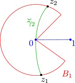
Figure 10: Rescaling and rotation of region of interest depicted in Figure 9. Region $B_{1}$ is a translation, rotation, and rescaling of $\widehat{B}_{\delta}$ such that $B_{1}$ has radius $1$. For $z\in B_{1}$, the quadrature formula must satisfy (200).

We define $B_{\delta}$ as

$$B_{\delta}=\big{\{}z:|\text{Arg}(z)|\geq\frac{\pi}{6},|z|\leq\delta\big{\}}.$$ (198)

Recall from Section 3.4 that $\gamma_{2}$, in the vicinity of $p_{2}$, always lies in $p_{2}+\widehat{B}_{\delta}$, where $\widehat{B}_{\delta}$ is a rotated version of $B_{\delta}$, such that the opening in $B_{\delta}$ is bisected by $C_{\rho}$ (see Figure 9). We note that, due to the same argument in Section 4.3.1, for $z$ outside of $B_{\delta}$ but elsewhere where the quadrature must hold, $z$ is well-separated from the domain of integration $C_{\rho}\setminus\widetilde{C}_{\rho}$ , meaning that a Gauss-Legendre quadrature accurately approximates the integral. Hence, for the remainder of this section we exclusively focus on developing a quadrature rule which approximates (197) for $z\in p_{2}+\widehat{B}_{\delta}$.

For convenience, we rotate, translate, and rescale $C_{\rho}\setminus\widetilde{C}_{\rho}$ and $p_{2}+\widehat{B}_{\delta}$ (see Figure 10), so that the segment $C_{\rho}\setminus\widetilde{C}_{\rho}$ is by approximated by the interval $[0,1]$ (i.e., it is translated by $p_{2}$, rotated, and scaled by a factor of $m^{2}$). Likewise, $\widecheck{\gamma_{2}}$ represents a similarly translated, rotated, and scaled copy of $\gamma_{2}$. Note that we associate $p_{2}$ with the point $x=0$ and the point $\widetilde{p}_{2}$ with $x=1$ (see Figure 10). Consider a quadrature rule $x_{i},\ldots,x_{n}$ and $w_{1},\ldots,w_{n}$ such that

$$\bigg{|}\int_{0}^{1}\frac{\rho(x)}{x-z}dx-\sum_{i=1}^{n}\frac{\rho(x_{i})}{x_{i}-z}w_{i}\bigg{|}<\epsilon$$ (199)

for all $z\in B_{1}$, where $\rho(x)$ is smooth. Such a quadrature, if used to approximate (197), will be accurate to precision $\epsilon$, for all $z\in p_{2}+\widehat{B}_{\delta}$. However, recall that we are integrating $R_{m}(z)$ given by (175) over $\gamma_{1}\cap E_{\widetilde{\rho}}^{o}$ and $\gamma_{2}\cap E_{\widetilde{\rho}}^{o}$. In the rotated and rescaled coordinates, this means that we are integrating $z\in\widecheck{\gamma}_{2}\subset B_{1}$, where $\widecheck{\gamma}_{2}$ starts at $z_{1}\in\partial B_{1}$ and ends at $z_{2}\in\partial B_{1}$, with $|z_{1}|=|z_{2}|=1$. We thus relax the requirement (199) to hold in $L^{1}(\widecheck{\gamma}_{2}\cap B_{1})$, meaning that the integral and the quadrature approximation in (199) can disagree on a set of measure $\epsilon$.

This allows us to relax (199) to the condition

$$\bigg{|}\int_{0}^{1}\frac{\rho(x)}{x-z}dz-\sum_{i=1}^{n}\frac{\rho(x_{i})}{x_{i}-z}w_{i}\bigg{|}<\frac{\epsilon}{|z|},$$ (200)

for $z\in B_{1}$. Thus, for each $\delta>0$, if $z\in B_{\delta}$, then the quadrature is accurate to within an error $\epsilon/\delta$. Since the length of $\widecheck{\gamma}_{2}\cap B_{\delta}$ is on the order $\delta$, the $L^{1}$ error in the quadrature is $\delta\cdot\epsilon/\delta=\epsilon$.

We can construct this quadrature by first sampling $z_{i}\in\partial B_{1}$, and then computing a generalized Gaussian quadrature (see [5]) on $x\in[0,1]$, where (200) is enforced on all the sampled $z_{i}$’s. By Cauchy’s theorem, if (200) holds on $\partial B_{1}$, then it will also hold on $B_{1}$. However, this still results in a quadrature rule with several hundred nodes. It turns out that far fewer nodes can be used, due to the following observation.

Recall that, in the integrand of (179), $R_{m}(z)$ is multiplied by a spherical wave term, denoted as $H(z)$, given by

$$H(z)=\frac{e^{-i\kappa\sqrt{1-\alpha z}}}{\sqrt{1-\alpha z}\sqrt{1-z^{2}}}.$$ (201)

Because $H(z)$ is smooth near $z=p_{2}$, we only need that

$$\bigg{|}\int_{\widecheck{\gamma}_{2}\cap B_{1}}\sigma(z)\int_{0}^{1}\frac{\rho(x)}{x-z}dxdz-\int_{\widecheck{\gamma}_{2}\cap B_{1}}\sigma(z)\sum_{i=1}^{n}\frac{\rho(x_{i})}{x_{i}-z}w_{i}dz\bigg{|}<\epsilon,$$ (202)

for all sufficiently smooth functions $\sigma(z)$. Since $\sigma(z)$ is smooth, it can be represented by a Taylor series of a small order $k$, so that

$$\sigma(z)\approx\sum_{j=0}^{k}a_{j}z^{j}.$$ (203)

Thus, inequality (202) becomes

$$\bigg{|}\int_{\widecheck{\gamma}_{2}\cap B_{1}}z^{j}\int_{0}^{1}\frac{\rho(x)}{x-z}dxdz-\int_{\widecheck{\gamma}_{2}\cap B_{1}}z^{j}\sum_{i=1}^{n}\frac{\rho(x_{i})}{x_{i}-z}w_{i}dz\bigg{|}<\epsilon,$$ (204)

for each $j=0,1,\ldots,k$. Exchanging the order of integration,

$$\bigg{|}\int_{0}^{1}\rho(x)\int_{\widecheck{\gamma}_{2}\cap B_{1}}\frac{z^{j}}{x-z}dzdx-\sum_{i=1}^{n}\rho(x_{i})\int_{\widecheck{\gamma}_{2}\cap B_{1}}\frac{z^{j}}{x_{i}-z}dz\,w_{i}\bigg{|}<\epsilon.$$ (205)

Recall from Section 2.6 that

$$\int_{\widecheck{\gamma}_{2}\cap B_{1}}\frac{z^{j}}{x-z}dz=\phi(x)+\psi(x)\log\Big{(}\frac{x-z_{1}}{x-z_{2}}\Big{)},$$ (206)

where $\phi$ and $\psi$ are polynomials of order $j$, and $z_{1}$ and $z_{2}$ are the endpoints of $\widecheck{\gamma}_{2}\cap B_{1}$. Due to the geometry of $B_{1}$, we have that

$$|z_{1}-x|\geq\frac{1}{2},\qquad|z_{2}-x|\geq\frac{1}{2},$$ (207)

for all $x\in[0,1]$. We also observe that the branch cut of

$$\log\bigg{(}\frac{x-z_{1}}{x-z_{2}}\bigg{)}$$ (208)

does not intersect $[0,1]$, so (208) smooth on $[0,1]$. Since $\rho(x)$ is smooth and (208) is smooth, we observe that the integrand in (205), given by

$$\rho(x)\int_{\widecheck{\gamma}_{2}\cap B_{1}}\frac{z^{j}}{x-z}dz,$$ (209)

is a smooth function of $x$ for $x\in[0,1]$. Hence, a Gauss-Legendre quadrature with $O(1)$ points will satisfy (205).

Because (205) is satisfied, (202) is satisfied, and so the contour deformation argument presented in Section 4.1.1 can be carried out without change, using a Gauss-Legendre quadrature with $O(1)$ points on $C_{\rho}\setminus\widetilde{C}_{\rho}$ and $O(m)$ points on $\widetilde{C}_{\rho}$.

4.3.3 The Error in the Approximation $R_{m}(z)$

In order to derive the approximation (178) to the Green’s function $G_{m}$, we approximated the Chebyshev polynomial $T_{m}(z)$ by the function $R_{m}(z)$, defined by (175) (see also (163) and (164)). Recall from Section 3.2.2 that, when $\rho=M^{1/m}$, we have that ${\lvert T_{m}(z)\rvert}\approx M$ for all $z\in E_{\rho}$. If the formula for $R_{m}(z)$ is evaluated numerically, then the integrand and summand in that formula will both have size approximately $M$, while the sum, $R_{m}(z)$, will have size approximately one for $z\in[-1,1]$. Thus, due to cancellation error, ${\lvert R_{m}(z)-T_{m}(z)\rvert}\approx M\epsilon$ for all $z\in[-1,1]$, where $\epsilon$ is equal to machine precision. This means that, for $\rho=M^{1/m}$, the approximation for $G_{m}$ given by formula (178) has an error of $M\epsilon$.

4.3.4 The Number of Quadrature Nodes on $\widetilde{C}_{\rho}$

In Section 4.3.2, we demonstrated that only $O(1)$ nodes are required on $C_{\rho}\setminus\widetilde{C}_{\rho}$. In Section 4.3.1, we showed that $O(m)$ nodes are required on $\widetilde{C}_{\rho}$ by pointing out that the distance from $\widetilde{C}_{\rho}$ to the nearest pole is $1/m^{2}$ at its endpoints and $\approx 1/m$ in the middle. We then used Corollary 3.1 and Remark 3.1 to state that the number of terms required to expand the integrand in (196) in Chebyshev polynomials is $O(m)$, which means that $O(m)$ nodes are needed in the corresponding quadrature formula.

In fact, Corollary 3.1 and Remark 3.1 provide a quantitative estimate for how many terms are required. If a function on a contour of length $2$ is analytic and bounded by $L$ on a region containing the contour, where the boundary of the region is separated from the contour by a distance of $(\log(M)/m)^{2}$ at the endpoints and $\log(M)/m$ in the middle, then the number of Chebyshev expansion coefficients required to approximate that function on the contour to precision $\epsilon$ is

$$k_{0}\approx m{(\log(2L)-\log(\epsilon))/\log(M)}.$$ (210)

When $\rho=M^{1/m}$, a straightforward modification of the argument in Section 4.3.1 shows that the distance from the contour $\widetilde{C}_{\rho}$ to the nearest pole is $(\log(M)/m)^{2}$ at its endpoints and $\approx\log(M)/m$ in the middle. Thus, if we take a slightly smaller region, say, $90\%$ the size, then $L\approx 10M$. Replacing $\epsilon$ in formula (210) by $M\epsilon$, since this is the minimum error we can hope to achieve (see Section 4.3.3), the estimate for the number of terms in the Chebyshev expansion of the integrand of (196) becomes

$$k_{0}\approx\frac{m}{0.9}{(\log(2\cdot 10M)-\log(M\epsilon))/\log(M)},$$ (211)

which simplifies to

$$k_{0}\approx 1.11m{(\log(20)-\log(\epsilon))/\log(M)}.$$ (212)

Taking $\epsilon=10^{-16}$, we compute the number of terms $k_{0}$ in the Chebyshev expansion required to approximate the integrand of (196) to precision $M\epsilon$ for $M=10,100,\ldots,10^{12}$ (see Table 1). Likewise, taking $\epsilon=10^{-34}$, we compute the number of terms $k_{0}$ for $M=10,100,\ldots,10^{15}$ (see Table 2). We note that, if $k_{0}$ Chebyshev expansion coefficients are required to approximate the integrand, then the integral (196) can be evaluated using a Gauss-Legendre quadrature with approximately $k_{0}/2$ points, since that a Gauss-Legendre quadrature integrates approximately twice as many polynomials as the number of quadrature points.

$M$	$M\epsilon$	$k_{0}$	$k_{0}/2$
10	$10^{-15}$	19.2m	9.6m
100	$10^{-14}$	9.6m	4.8m
$10^{3}$	$10^{-13}$	6.4m	3.2m
$10^{6}$	$10^{-10}$	3.2m	1.6m
$10^{9}$	$10^{-7}$	2.13m	1.07m
$10^{12}$	$10^{-4}$	1.6m	0.8m

Table 1: The required number of Gauss-Legendre nodes on $\widetilde{C}_{\rho}$ to approximate  (196), in double precision. In this table, $k_{0}/2$ is the required number of nodes, $\epsilon=10^{-16}$, and $\rho=M^{1/m}$.

$M$	$M\epsilon$	$k_{0}$	$k_{0}/2$
10	$10^{-33}$	39.2m	19.6m
100	$10^{-32}$	19.6m	9.8m
$10^{3}$	$10^{-31}$	13.1m	6.53m
$10^{6}$	$10^{-28}$	6.53m	3.27m
$10^{9}$	$10^{-25}$	4.35m	2.18m
$10^{12}$	$10^{-22}$	3.27m	1.63m
$10^{15}$	$10^{-19}$	2.61m	1.31m

Table 2: The required number of Gauss-Legendre nodes on $\widetilde{C}_{\rho}$ to approximate (196), in quadruple precision. In this table, $k_{0}/2$ is the required number of nodes, $\epsilon=10^{-34}$, and $\rho=M^{1/m}$.

Finally, we observe that, in practice, we can place a single $O(m)$ Gauss-Legendre quadrature with $k_{0}/2$ nodes on the entire contour $C_{\rho}$, rather than placing two $O(1)$ quadratures on each part of $C_{\rho}\setminus\widetilde{C}_{\rho}$ and one $O(m)$ quadrature on $\widetilde{C}_{\rho}$. Also, we note that, in practice, the minimum number of quadrature nodes required to achieve the accuracy $M\epsilon$ matches the estimates in Tables 1 and 2 very closely.

4.4 Summary of the Algorithm

Recall from Section 1.1 that $G_{m}$ is a function of $\kappa$, $m$, and $\alpha$. Recall also that $\alpha$ can be determined from $\beta_{-}$ (see formula 11)), and vice versa. We consider $G_{m}$ as a function of $\kappa$, $m$, and $\beta_{1}$. We compute $G_{m}$ as follows. Recall from Section 4.2 the formula for $G_{m}$,

$$\begin{split}G_{m}\approx\frac{-4}{\sqrt{\alpha}}\int_{0}^{\tau_{1}}\frac{F_{1}(\tau)}{\sqrt{\tau^{2}+2i\beta_{-}}}d\tau+\frac{4i}{\sqrt{\alpha}}\int_{0}^{\tau_{2}}\frac{F_{2}(\tau)}{\sqrt{\tau^{2}+2i\beta_{+}}}d\tau\\ +\sum_{i=1}^{n}\frac{e^{-i\kappa\sqrt{1-\alpha v_{i}}}}{\sqrt{1-\alpha v_{i}}\sqrt{1-v_{i}^{2}}}T_{m}(v_{i})dv_{i}w_{i},\end{split}$$ (213)

where $F_{1}(\tau)$ and $F_{2}(\tau)$ are smooth functions corresponding to the $\gamma_{1}$ and $\gamma_{2}$ contours, respectively defined by (133) and (138), $\tau_{1}$ and $\tau_{2}$ are positive parameters such that $\gamma_{1}(\tau_{1})$ and $\gamma_{2}(\tau_{2})$ intersect $E_{\rho}$ (see Section 3.7) , respectively, $T_{m}$ is the $m$th order Chebyshev polynomial, and

$$\beta_{-}=\sqrt{1/\alpha-1},\qquad\beta_{+}=\sqrt{1/\alpha+1}.$$ (214)

Recall from Section 3.4 that both $\gamma_{1}\cap E_{\rho}$ and $\gamma_{2}\cap E_{\rho}$ have length $\approx 1/m^{2}$. Hence, $T_{m}(z)$ oscillates at most once along each contour. By construction, on Gustafsson’s contours (see Section 3.1.1), the spherical wave portion of the integrand does not oscillate. Hence, the entire integrand oscillates at most once. By the argument in Section 4.2 the integrand associated with the $\gamma_{2}$ contour is always smooth and hence can be evaluated with an $O(1)$ Gauss-Legendre quadrature.

The integrand associated with the contour $\gamma_{1}$ has a singularity for $\beta_{-}\approx 0$. For this case, we follow the method in Section 4.2 and evaluate the portion near the singularity by expanding the function $F_{1}(\tau)$ into its Taylor series, then use the recurrence described in Section 4.2.1. Due to the smoothness of $F_{1}(\tau)$, this integral is computed with an $O(1)$ Gauss-Legendre quadrature. The remainder of the integral is smooth and oscillates at most once, and hence is evaluated with an $O(1)$ Gauss-Legendre quadrature. Hence, both integrals in (213) are evaluated in $O(1)$ operations.

The remaining term in (213) is a sum of residues evaluated on $C_{\rho}$, where $C_{\rho}$ denotes the portion of a Bernstein ellipse connecting $\gamma_{1}$ and $\gamma_{2}$ (see Section 4.1). We select the residues $v_{1},\ldots,v_{n}$ and weights $w_{1},\ldots,w_{n}$ by constructing a quadrature which approximates

$$\oint_{C_{\rho}}\frac{T_{m}(v)}{v-z}dv,$$ (215)

which holds for values of $z$ relevant to the evaluation of $G_{m}$ (see Section 4.3.2). By the argument in Section 4.3, this is accomplished using $O(m)$ Gauss Legendre nodes on $C_{\rho}$.

Therefore, the entire cost of our algorithm for $G_{m}$ is $O(m)$ and completely independent of both $\kappa$ and $\beta_{-}$. Lastly, since the algorithm is entirely quadrature based, it is embarrassingly parallelizable. Finally, we note that implementing this algorithm requires certain numerical issues to be treated with care, which we describe in Section 4.5.

4.5 Numerical Miscellanea

This section contains various facts required for the accurate evaluation of some of the quantities and formulas used by the numerical algorithm of this manuscript.

4.5.1 Evaluating the Semi-major and Semi-minor Axes of the Bernstein Ellipse

We will need to compute the quantities $a-1$ and $b$, where $a$ is the semi-major axis of the Bernstein ellipse $E_{\rho}$ described in Section 2.2 and $b$ is the semi-minor axis. When $\rho\approx 1$, we have that $a\approx 1$, so computing $a-1\approx 0$ directly from $a$ will result in a large cancellation error. Likewise, when $\rho\approx 1$, we have that $b\approx 0$, so computing it from formula (45) will also result in cancellation error. Instead of computing

$$\rho=M^{\frac{1}{m}},$$ (216)

as in formula (89), we instead compute the value of the semi-minor axis $b$ directly using the formula

$$b=\sinh(\log(M)/m)=\frac{1}{2}(e^{\log(M)/m}-e^{-\log(M)/m})=\frac{1}{2}(\rho-\frac{1}{\rho}).$$ (217)

which can be done stably even when $m$ is very large. We then compute the value of the semi-major axis $a$ from $b$ using the formula

$$a=\sqrt{b^{2}+1}=\cosh(\log(M)/m)=\frac{1}{2}(\rho+\frac{1}{\rho}).$$ (218)

The value of $a-1$ is also given by the formula

$$a-1=\frac{b^{2}}{a+1},$$ (219)

and is likewise derived from identities involving the hyperbolic functions.

4.5.2 The Evaluation of $\beta_{-}$ when $\alpha\approx 1$

When $\alpha\approx 1$, the quantity $\beta_{-}=\sqrt{1/\alpha-1}$ will be computed with a very large cancellation error. Thus, instead of using $\alpha$ as an input parameter to our algorithm, we use $\beta_{-}$. The quantity $\alpha$ can be obtained from $\beta_{-}$ by the formula $\alpha=1/(\beta_{-}^{2}+1)$, and $\beta_{-}$ can be evaluated to full relative precision from (14).

4.5.3 The Evaluation of the Quantity $\sqrt{1-\alpha z}$ when $\alpha\approx 1$ and $z\approx 1$

Sometimes we will need to evaluate the quantity $\sqrt{1-\alpha z}$ on Gustafsson’s contours when $\alpha\approx 1$ and $z\approx 1$. As mentioned in Section 1.1, we use $\beta_{-}$ as an input parameter to prevent a loss of accuracy. With the parameterization $z=\widetilde{\gamma}_{1}(\tau)$ of the contour $\gamma_{1}$, given by (127), we have

$$\sqrt{1-\alpha\widetilde{\gamma}_{1}(\tau)}=-i\sqrt{\alpha}(\tau^{2}+i\beta_{-}),$$ (220)

as stated in (128). This formula can be evaluated to relative precision when $\beta_{-}\approx 0$ and $\tau\approx 0$ (equivalently, when $\alpha\approx 1$ and $z\approx 1$).

4.5.4 The Evaluation of the Intersection Points $p_{1}$ and $p_{2}$

In Section 3.7, we determine the intersection points of the Gustafsson contours $\gamma_{1}$ and $\gamma_{2}$ with the Bernstein ellipse $E_{\rho}$, in both the Bernstein ellipse parameter $\theta$ and Gustafsson’s contours’ parameter $\tau$. These formulas all involve solving a quadratic equation. To solve it accurately, we use the observation in Section 2.7.

4.5.5 The Evaluation of $\arccos(s)$ for $s\approx 1$

In the construction of the intersection points of the Gustaffson contours $\gamma_{1}$ and $\gamma_{2}$ with the Bernstein ellipse $E_{\rho}$, in the Bernstein ellipse parameter $\theta$, it is sometimes the case that $\theta=\arccos(s)\approx 0$ and $s\approx 1$ in formula (146). The condition number of $\arccos(s)$ becomes infinite near $s=1$, so a straightforward application of the formula results in a loss of accuracy. We observe that the function $\arccos(1+z)$ can be evaluated accurately for $z\approx 0$ (by, for example, Taylor series). Thus, instead of solving the quadratic equation for $s$, we solve for $s-1$, and then evalate $\arccos(1+z)$ for $z=s-1$.

4.5.6 The Evaluation of $T_{m}(z)$ when $z\approx\pm 1$

Since we use the parameterizations $z=\widetilde{\gamma}_{1}(\tau)$ and $z=\widetilde{\gamma}_{2}(\tau)$ for Gustafsson’s contours, we are able to evaluate $z-1$ and $z+1$ to full relative precision on $\gamma_{1}$ and $\gamma_{2}$, respectively. However, the formula

$$T_{m}(z)=\cos(m\arccos(z))$$ (221)

requires the evaluation of $\arccos(z)$ near $z=1$, where its condition number is infinite. Instead, we observe that $\arccos(1+z)$ can be evaluated to full relative accuracy near $z=0$ (using, for example, Taylor series). Thus, we evaluate

$$T_{m}(z)=\cos(m\arccos(1+w))$$ (222)

accurately for $w=z-1\approx 0$ with $z\in\gamma_{1}$. Likewise, we use the fact that $\arccos(-z)=\pi-\arccos(z)$ to evaluate

$$T_{m}(z)=(-1)^{m}\cos(m\arccos(1+w))$$ (223)

accurately for $w=-z-1\approx 0$ with $z\in\gamma_{2}$.

4.5.7 The Limits of Integration on Gustafsson’s Contours

In order to approximate the modal Green’s function $G_{m}$ using formula (213), it is necessary to evaluate the integrals

$$\int_{0}^{\tau_{1}}\frac{F_{1}(\tau)}{\sqrt{\tau^{2}+2i\beta_{-}}}d\tau,\qquad\text{with}\qquad F_{1}(\tau)=\frac{e^{-i\kappa\sqrt{1-\alpha\widetilde{\gamma_{1}}(\tau)}}}{\sqrt{1+\widetilde{\gamma_{1}}(\tau)}}T_{m}(\widetilde{\gamma_{1}}(\tau)),$$ (224)

and

$$\int_{0}^{\tau_{2}}\frac{F_{2}(\tau)}{\sqrt{\tau^{2}+2i\beta_{+}}}d\tau,\qquad\text{with}\qquad F_{2}(\tau)=\frac{e^{-i\kappa\sqrt{1-\alpha\widetilde{\gamma_{2}}(\tau)}}}{\sqrt{1+\widetilde{\gamma_{2}}(\tau)}}T_{m}(\widetilde{\gamma_{2}}(\tau)),$$ (225)

where $\widetilde{\gamma}_{1}(\tau_{1})$ and $\widetilde{\gamma}_{2}(\tau_{2})$ are, respectively, the intersection points of $\gamma_{1}$ and $\gamma_{2}$ with $E_{\rho}$ (see (133) and (138). The integrands decay exponentially in $\tau$ at a rate proportional to $\kappa$. Thus, when $\kappa$ is large, care must be taken to choose the domains of integration when evaluating the integrals numerically.

In order to evaluate the integrals (224) and (225) to within an error of $M\epsilon$ (see Section 4.3.3), the integrals only need to be evaluated over values of $\tau$ for which $F_{1}(\tau)\geq M\epsilon$ and $F_{2}(\tau)\geq M\epsilon$, respectively. Since $\widetilde{\gamma}_{1}(\tau)\in E_{\rho}^{o}$ for all $\tau\in[0,\tau_{1})$ and $\widetilde{\gamma}_{2}(\tau)\in E_{\rho}^{o}$ for all $\tau\in[0,\tau_{2})$, by (87), it follows that, when $\rho=M^{1/m}$, ${\lvert T_{m}(\widetilde{\gamma}_{1}(\tau))\rvert}<M$ for $\tau\in[0,\tau_{1})$ and ${\lvert T_{m}(\widetilde{\gamma}_{2}(\tau))\rvert}<M$ for $\tau\in[0,\tau_{2})$. We observe then that

$$F_{1}(\tau)\approx Me^{-i\kappa\sqrt{1-\alpha\widetilde{\gamma}_{1}(\tau)}}\qquad\text{and}\qquad F_{2}(\tau)\approx Me^{-i\kappa\sqrt{1-\alpha\widetilde{\gamma}_{2}(\tau)}}.$$ (226)

By (129),

$$\sqrt{1-\alpha\widetilde{\gamma}_{1}(\tau)}=-i\sqrt{\alpha}(\tau^{2}+i\beta_{-}),$$ (227)

and, likewise,

$$\sqrt{1-\alpha\widetilde{\gamma}_{2}(\tau)}=-i\sqrt{\alpha}(\tau^{2}+i\beta_{+}).$$ (228)

Thus,

$${\lvert e^{-i\kappa\sqrt{1-\alpha\widetilde{\gamma}_{1}(\tau)}}\rvert}={\lvert e^{-\kappa\sqrt{\alpha}\tau^{2}}\rvert},$$ (229)

and

$${\lvert e^{-i\kappa\sqrt{1-\alpha\widetilde{\gamma}_{2}(\tau)}}\rvert}={\lvert e^{-\kappa\sqrt{\alpha}\tau^{2}}\rvert}.$$ (230)

Solving the equation

$$e^{-\kappa\sqrt{\alpha}\tau^{2}}=\epsilon$$ (231)

for $\tau$, we arrive at the formula

$$\tau_{c}=\sqrt{\frac{-\log(\epsilon)}{\kappa\sqrt{\alpha}}},$$ (232)

from which we see that $F_{1}(\tau_{c})\approx M\epsilon$ and $F_{2}(\tau_{c})\approx M\epsilon$. Thus, we evaluate the integrals (224) and (225) over Gustafsson’s contours only on the intervals $[0,\min(\tau_{1},\tau_{c}))$ and $[0,\min(\tau_{2},\tau_{c}))$, respectively. Hence, rather than evaluate (224) and (225), we instead evaluate

$$\int_{0}^{\min(\tau_{1},\tau_{c})}\frac{F_{1}(\tau)}{\sqrt{\tau^{2}+2i\beta_{-}}}d\tau\qquad\text{and}\qquad\int_{0}^{\min(\tau_{2},\tau_{c})}\frac{F_{2}(\tau)}{\sqrt{\tau^{2}+2i\beta_{+}}}d\tau.$$ (233)

5 Numerical Experiments

In Sections 5.1-5.4 we characterize the speed and accuracy of our method. Importantly, as demonstrated below, we achieve full precision for all possible ranges of $\beta_{-}$ and $\kappa$, and our algorithm’s performance is completely independent of $\beta_{-}$ and $\kappa$.

We use adaptive integration applied to (63) as the gold standard, and measure the error of our algorithm by comparing the two results. We use the change of variables $\phi=x^{3}$, $d\phi=3x^{2}dx$, to ensure that adaptive integration is accurate when $\alpha\approx 1$. We compute the $1-\alpha\cos(\phi)$ term using the double angle formula to avoid cancellation error. The error in evaluating the modal Green’s function for very large $\kappa$ is not measured, as adaptive integration is too expensive and no prior method can compute the modal Green’s function for large $\kappa$.

An implementation of the previously described algorithm was written in Fortran 77. In our implementation, we chose $M=100$, and used $5m$ quadrature nodes on $C_{\rho}$ in double precision, and $11m$ quadrature nodes on $C_{\rho}$ in extended precision (see Section 4.3.4). The timing and performance experiments in Sections 5.1–5.3 were performed using a consumer laptop with a four-core 2.6 GHz Intel i7 processor running a timing script in MATLAB 2018b with two threads. The parallel computing experiment in Section 5.4 was run on a server with a 16-core Intel Xeon 2.9 GHz processor.

5.0.1 The Interpretation of $\beta_{-}$ and $\kappa$

Recall from Section 1.1 that the modal Green’s function can be thought of as a function of four parameters: $m$, $k$, $\alpha$, and $R_{0}$. After the introduction of the parameters $\kappa$ and $\beta_{-}$ (see formula (10)), the $R_{0}$ term exclusively appears as a $1/R_{0}$ scaling outside the integral. Hence, with this parameterization, $R_{0}$ is of no independent consequence to the performance of our algorithm, so we only characterize our algorithm’s performance as a function of $\kappa$, $\beta_{-}$, and $m$. Recall also that $\beta_{-}$ is defined as

$$\beta_{-}=\frac{\Delta}{\rho_{0}},$$ (234)

where $\Delta$ is the minimum source-to-target distance and $\rho_{0}=2rr^{\prime}$, with $r$ and $r^{\prime}$ being the radial distances of the source and target in cylindrical coordinates. Recall finally from Section 1.1 that $\kappa$ is defined as

$$\kappa=kR_{0}.$$ (235)

5.1 Performance of the Algorithm with Varying Source-to-Target Distance

We examined the performance of our algorithm over a wide range of source-to-target distances. As shown in Table 3 and Table 4, our algorithm’s performance is independent of $\beta_{-}$.

	$\kappa=10,000,\,m=10$		$\kappa=10,000,\,m=1000$
$\beta_{-}$	Evaluation Time	Absolute Error	Evaluation Time	Absolute Error
$10^{15}$	4.66$\times 10^{-5}$ secs	1.47$\times 10^{-13}$	1.33$\times 10^{-3}$ secs	7.29$\times 10^{-13}$
$10^{12}$	4.76$\times 10^{-5}$ secs	1.53$\times 10^{-13}$	1.34$\times 10^{-3}$ secs	7.29$\times 10^{-13}$
$10^{9}$	4.73$\times 10^{-5}$ secs	1.46$\times 10^{-13}$	1.34$\times 10^{-3}$ secs	7.29$\times 10^{-13}$
$10^{6}$	5.00$\times 10^{-5}$ secs	2.55$\times 10^{-11}$	1.41$\times 10^{-3}$ secs	2.11$\times 10^{-12}$
$10^{3}$	4.89$\times 10^{-5}$ secs	6.03$\times 10^{-12}$	1.41$\times 10^{-3}$ secs	2.64$\times 10^{-12}$
$10^{0}$	3.76$\times 10^{-5}$ secs	3.34$\times 10^{-14}$	1.44$\times 10^{-3}$ secs	4.71$\times 10^{-13}$
$10^{-3}$	3.57$\times 10^{-5}$ secs	3.43$\times 10^{-14}$	1.44$\times 10^{-3}$ secs	1.79$\times 10^{-12}$
$10^{-6}$	3.51$\times 10^{-5}$ secs	3.92$\times 10^{-14}$	1.44$\times 10^{-3}$ secs	3.43$\times 10^{-13}$
$10^{-9}$	3.59$\times 10^{-5}$ secs	5.50$\times 10^{-14}$	1.44$\times 10^{-3}$ secs	5.27$\times 10^{-13}$
$10^{-12}$	3.52$\times 10^{-5}$ secs	3.33$\times 10^{-14}$	1.44$\times 10^{-3}$ secs	5.28$\times 10^{-13}$
$10^{-15}$	3.46$\times 10^{-5}$ secs	1.69$\times 10^{-14}$	1.44$\times 10^{-3}$ secs	4.81$\times 10^{-13}$
$10^{-18}$	3.45$\times 10^{-5}$ secs	3.95$\times 10^{-14}$	1.44$\times 10^{-3}$ secs	4.84$\times 10^{-13}$
$10^{-21}$	3.44$\times 10^{-5}$ secs	6.63$\times 10^{-14}$	1.44$\times 10^{-3}$ secs	5.11$\times 10^{-13}$

Table 3: The evaluation of the modal Green’s function in double precision for a large wavenumber ($\kappa=10,000$). The error is evaluated by using adaptive Gaussian quadrature as the gold standard.

	$\kappa=10,000,\,m=10$		$\kappa=10,000,\,m=1000$
$\beta_{-}$	Evaluation Time	Absolute Error	Evaluation Time	Absolute Error
$10^{15}$	6.62$\times 10^{-3}$ secs	1.03$\times 10^{-30}$	2.14$\times 10^{-1}$ secs	2.11$\times 10^{-30}$
$10^{12}$	6.51$\times 10^{-3}$ secs	1.73$\times 10^{-29}$	2.10$\times 10^{-1}$ secs	2.24$\times 10^{-30}$
$10^{9}$	6.51$\times 10^{-3}$ secs	1.58$\times 10^{-29}$	2.11$\times 10^{-1}$ secs	1.44$\times 10^{-30}$
$10^{6}$	6.88$\times 10^{-3}$ secs	8.94$\times 10^{-30}$	2.10$\times 10^{-1}$ secs	1.58$\times 10^{-30}$
$10^{3}$	6.88$\times 10^{-3}$ secs	1.78$\times 10^{-29}$	2.11$\times 10^{-1}$ secs	1.99$\times 10^{-30}$
$10^{0}$	5.82$\times 10^{-3}$ secs	2.89$\times 10^{-32}$	2.11$\times 10^{-1}$ secs	6.59$\times 10^{-31}$
$10^{-3}$	5.84$\times 10^{-3}$ secs	2.31$\times 10^{-32}$	2.11$\times 10^{-1}$ secs	1.07$\times 10^{-30}$
$10^{-6}$	5.74$\times 10^{-3}$ secs	2.06$\times 10^{-31}$	2.11$\times 10^{-1}$ secs	1.82$\times 10^{-30}$
$10^{-9}$	6.25$\times 10^{-3}$ secs	3.45$\times 10^{-33}$	2.12$\times 10^{-1}$ secs	2.63$\times 10^{-31}$
$10^{-12}$	6.27$\times 10^{-3}$ secs	2.07$\times 10^{-32}$	2.12$\times 10^{-1}$ secs	1.55$\times 10^{-31}$
$10^{-15}$	6.22$\times 10^{-3}$ secs	9.65$\times 10^{-32}$	2.12$\times 10^{-1}$ secs	5.53$\times 10^{-31}$
$10^{-18}$	6.06$\times 10^{-3}$ secs	1.58$\times 10^{-31}$	2.11$\times 10^{-1}$ secs	5.60$\times 10^{-31}$
$10^{-21}$	5.92$\times 10^{-3}$ secs	2.18$\times 10^{-31}$	2.11$\times 10^{-1}$ secs	6.36$\times 10^{-31}$

Table 4: The evaluation of the modal Green’s function in quadruple precision for a large wavenumber ($\kappa=10,000$). The error is evaluated by using adaptive Gaussian quadrature as the gold standard.

5.2 Performance of the Algorithm with Varying $\kappa$

We examined the performance of our algorithm over a wide range of values for $\kappa$. As shown in Tables 5-8, our algorithm’s performance is independent of $\kappa$.

	$\beta_{-}=1\,,m=10$		$\beta_{-}=1\,,m=1000$
$\kappa$	Evaluation Time	Absolute Error	Evaluation Time	Absolute Error
$10^{-6}$	1.22$\times 10^{-4}$ secs	1.45$\times 10^{-13}$	1.84$\times 10^{-3}$ secs	2.05$\times 10^{-12}$
$10^{-3}$	6.26$\times 10^{-5}$ secs	1.50$\times 10^{-13}$	1.64$\times 10^{-3}$ secs	2.05$\times 10^{-12}$
$10^{0}$	6.08$\times 10^{-5}$ secs	1.61$\times 10^{-13}$	1.66$\times 10^{-3}$ secs	2.02$\times 10^{-12}$
$10^{1}$	1.36$\times 10^{-4}$ secs	2.71$\times 10^{-14}$	2.50$\times 10^{-3}$ secs	1.83$\times 10^{-12}$
$10^{2}$	1.02$\times 10^{-4}$ secs	4.94$\times 10^{-15}$	2.43$\times 10^{-3}$ secs	2.23$\times 10^{-12}$
$10^{3}$	4.56$\times 10^{-5}$ secs	1.30$\times 10^{-14}$	1.73$\times 10^{-3}$ secs	1.51$\times 10^{-12}$
$10^{4}$	3.89$\times 10^{-5}$ secs	3.34$\times 10^{-14}$	1.69$\times 10^{-3}$ secs	1.03$\times 10^{-12}$
$10^{5}$	3.94$\times 10^{-5}$ secs	2.25$\times 10^{-14}$	1.70$\times 10^{-3}$ secs	5.05$\times 10^{-13}$
$10^{6}$	4.15$\times 10^{-5}$ secs	2.75$\times 10^{-13}$	1.75$\times 10^{-3}$ secs	3.32$\times 10^{-13}$
$10^{7}$	3.78$\times 10^{-5}$ secs	–	8.39$\times 10^{-4}$ secs	–
$10^{8}$	3.91$\times 10^{-5}$ secs	–	8.33$\times 10^{-4}$ secs	–
$10^{9}$	4.46$\times 10^{-5}$ secs	–	8.23$\times 10^{-4}$ secs	–
$10^{12}$	3.77$\times 10^{-5}$ secs	–	8.14$\times 10^{-4}$ secs	–
$10^{15}$	4.46$\times 10^{-5}$ secs	–	8.18$\times 10^{-4}$ secs	–
$10^{18}$	3.98$\times 10^{-5}$ secs	–	8.33$\times 10^{-4}$ secs	–

Table 5: The evaluation of the modal Green’s function in double precision for varying $\kappa$ ($\beta_{-}=1$). The error is evaluated by using adaptive Gaussian quadrature as the gold standard. Note for $\kappa>10^{6}$, the resource requirements of prior methods becomes excessive.

	$\beta_{-}=1\,,m=10$		$\beta_{-}=1\,,m=1000$
$\kappa$	Evaluation Time	Absolute Error	Evaluation Time	Absolute Error
$10^{-6}$	7.17$\times 10^{-3}$ secs	4.06$\times 10^{-31}$	2.07$\times 10^{-1}$ secs	1.12$\times 10^{-30}$
$10^{-3}$	6.43$\times 10^{-3}$ secs	3.99$\times 10^{-31}$	2.07$\times 10^{-1}$ secs	1.12$\times 10^{-30}$
$10^{0}$	6.92$\times 10^{-3}$ secs	3.94$\times 10^{-31}$	2.09$\times 10^{-1}$ secs	1.20$\times 10^{-30}$
$10^{1}$	7.09$\times 10^{-3}$ secs	1.34$\times 10^{-31}$	2.11$\times 10^{-1}$ secs	9.06$\times 10^{-31}$
$10^{2}$	6.93$\times 10^{-3}$ secs	7.74$\times 10^{-34}$	2.10$\times 10^{-1}$ secs	1.32$\times 10^{-30}$
$10^{3}$	6.81$\times 10^{-3}$ secs	9.49$\times 10^{-33}$	2.11$\times 10^{-1}$ secs	1.01$\times 10^{-30}$
$10^{4}$	5.79$\times 10^{-3}$ secs	2.89$\times 10^{-32}$	2.12$\times 10^{-1}$ secs	6.59$\times 10^{-31}$
$10^{5}$	5.78$\times 10^{-3}$ secs	1.59$\times 10^{-31}$	2.12$\times 10^{-1}$ secs	6.05$\times 10^{-31}$
$10^{6}$	5.76$\times 10^{-3}$ secs	2.23$\times 10^{-31}$	2.11$\times 10^{-1}$ secs	4.69$\times 10^{-31}$
$10^{7}$	5.76$\times 10^{-3}$ secs	–	2.11$\times 10^{-1}$ secs	–
$10^{8}$	5.82$\times 10^{-3}$ secs	–	1.52$\times 10^{-1}$ secs	–
$10^{9}$	5.72$\times 10^{-3}$ secs	–	1.52$\times 10^{-1}$ secs	–
$10^{12}$	5.72$\times 10^{-3}$ secs	–	1.52$\times 10^{-1}$ secs	–
$10^{15}$	5.70$\times 10^{-3}$ secs	–	1.52$\times 10^{-1}$ secs	–
$10^{18}$	5.70$\times 10^{-3}$ secs	–	1.52$\times 10^{-1}$ secs	–

Table 6: The evaluation of the modal Green’s function in quadruple precision for a for varying $\kappa$ with large source-to-target distance ($\beta_{-}=1$). The error is evaluated by using adaptive Gaussian quadrature as the gold standard. Note for $\kappa>10^{6}$, the resource requirements of prior methods becomes excessive.

	$\beta_{-}=10^{-12}\,,m=10$		$\beta_{-}=10^{-12}\,,m=1000$
$\kappa$	Evaluation Time	Absolute Error	Evaluation Time	Absolute Error
$10^{-6}$	4.49$\times 10^{-5}$ secs	3.08$\times 10^{-13}$	1.34$\times 10^{-3}$ secs	2.90$\times 10^{-11}$
$10^{-3}$	4.45$\times 10^{-5}$ secs	2.90$\times 10^{-13}$	1.37$\times 10^{-3}$ secs	2.88$\times 10^{-11}$
$10^{0}$	4.77$\times 10^{-5}$ secs	1.90$\times 10^{-13}$	1.40$\times 10^{-3}$ secs	2.84$\times 10^{-11}$
$10^{1}$	4.79$\times 10^{-5}$ secs	4.35$\times 10^{-14}$	1.41$\times 10^{-3}$ secs	2.74$\times 10^{-11}$
$10^{2}$	4.61$\times 10^{-5}$ secs	1.80$\times 10^{-14}$	1.43$\times 10^{-3}$ secs	2.29$\times 10^{-11}$
$10^{3}$	3.57$\times 10^{-5}$ secs	1.07$\times 10^{-14}$	1.44$\times 10^{-3}$ secs	4.19$\times 10^{-12}$
$10^{4}$	3.49$\times 10^{-5}$ secs	3.33$\times 10^{-14}$	1.43$\times 10^{-3}$ secs	5.28$\times 10^{-13}$
$10^{5}$	3.46$\times 10^{-5}$ secs	1.50$\times 10^{-13}$	1.44$\times 10^{-3}$ secs	6.58$\times 10^{-13}$
$10^{6}$	3.41$\times 10^{-5}$ secs	5.11$\times 10^{-13}$	1.45$\times 10^{-3}$ secs	3.04$\times 10^{-13}$
$10^{7}$	3.48$\times 10^{-5}$ secs	–	7.88$\times 10^{-4}$ secs	–
$10^{8}$	3.43$\times 10^{-5}$ secs	–	7.87$\times 10^{-4}$ secs	–
$10^{9}$	3.38$\times 10^{-5}$ secs	–	7.87$\times 10^{-4}$ secs	–
$10^{12}$	3.22$\times 10^{-5}$ secs	–	7.85$\times 10^{-4}$ secs	–
$10^{15}$	3.38$\times 10^{-5}$ secs	–	7.87$\times 10^{-4}$ secs	–
$10^{18}$	3.33$\times 10^{-5}$ secs	–	7.85$\times 10^{-4}$ secs	–

Table 7: The evaluation of the modal Green’s function in double precision for varying $\kappa$ with small source-to-target distance ($\beta_{-}=10^{-12}$). The error is evaluated by using adaptive Gaussian quadrature as the gold standard. Note for $\kappa>10^{6}$, the resource requirements of prior methods becomes excessive.

	$\beta_{-}=10^{-12}\,,m=10$		$\beta_{-}=10^{-12}\,,m=1000$
$\kappa$	Evaluation Time	Absolute Error	Evaluation Time	Absolute Error
$10^{-6}$	7.23$\times 10^{-3}$ secs	7.06$\times 10^{-31}$	2.08$\times 10^{-1}$ secs	5.75$\times 10^{-29}$
$10^{-3}$	7.53$\times 10^{-3}$ secs	7.12$\times 10^{-31}$	2.08$\times 10^{-1}$ secs	5.75$\times 10^{-29}$
$10^{0}$	7.16$\times 10^{-3}$ secs	6.54$\times 10^{-31}$	2.10$\times 10^{-1}$ secs	5.70$\times 10^{-29}$
$10^{1}$	7.53$\times 10^{-3}$ secs	8.03$\times 10^{-32}$	2.11$\times 10^{-1}$ secs	5.56$\times 10^{-29}$
$10^{2}$	7.09$\times 10^{-3}$ secs	5.00$\times 10^{-32}$	2.11$\times 10^{-1}$ secs	4.55$\times 10^{-29}$
$10^{3}$	6.25$\times 10^{-3}$ secs	6.41$\times 10^{-32}$	2.12$\times 10^{-1}$ secs	7.93$\times 10^{-30}$
$10^{4}$	6.23$\times 10^{-3}$ secs	2.07$\times 10^{-32}$	2.11$\times 10^{-1}$ secs	1.55$\times 10^{-31}$
$10^{5}$	6.21$\times 10^{-3}$ secs	1.43$\times 10^{-31}$	2.12$\times 10^{-1}$ secs	2.21$\times 10^{-31}$
$10^{6}$	6.21$\times 10^{-3}$ secs	2.37$\times 10^{-31}$	2.12$\times 10^{-1}$ secs	3.88$\times 10^{-31}$
$10^{7}$	6.25$\times 10^{-3}$ secs	–	1.52$\times 10^{-1}$ secs	–
$10^{8}$	6.22$\times 10^{-3}$ secs	–	1.53$\times 10^{-1}$ secs	–
$10^{9}$	6.19$\times 10^{-3}$ secs	–	1.52$\times 10^{-1}$ secs	–
$10^{12}$	5.78$\times 10^{-3}$ secs	–	1.52$\times 10^{-1}$ secs	–
$10^{15}$	5.72$\times 10^{-3}$ secs	–	1.52$\times 10^{-1}$ secs	–
$10^{18}$	5.69$\times 10^{-3}$ secs	–	1.52$\times 10^{-1}$ secs	–

Table 8: The evaluation of the modal Green’s function in quadruple precision for varying $\kappa$ with small source-to-target distance ($\beta_{-}=10^{-12}$). The error is evaluated by using adaptive Gaussian quadrature as the gold standard. Note for $\kappa>10^{6}$, the resource requirements of prior methods becomes excessive.

5.3 Performance of the Algorithm with Varying Fourier Mode ($m$)

We examined the performance of our algorithm over a wide range of Fourier modes (represented by the parameter $m$). Because the number of points in the quadrature scales linearly with $m$, as demonstrated by Table 9, evaluation time scales linearly with the Fourier mode. Recall from the introduction of this section that the evaluation was performed on a four-core processor using two threads.

$m$	Evaluation Time
1	3.88$\times 10^{-5}$ secs
10	5.56$\times 10^{-5}$ secs
$10^{2}$	1.75$\times 10^{-4}$ secs
$10^{3}$	1.46$\times 10^{-3}$ secs
$10^{4}$	1.43$\times 10^{-2}$ secs
$10^{5}$	1.37$\times 10^{-1}$ secs
$10^{6}$	1.36$\times 10^{0}$ secs
$10^{7}$	1.29$\times 10^{1}$ secs

Table 9: The evaluation time of the modal Green’s function in double precision for varying $m$ ($\beta_{-}=10^{-12},\kappa=10,000$).

5.4 Parallelization of the Algorithm

The cost of our algorithm is $O(m)$ and does not depend on $\kappa$ or $\beta_{-}$ (see Section 4.4). Because our algorithm is quadrature based, it is embarrassingly parallelizable.

We measured the algorithm’s performance on a server with a 16-core Intel Xeon 2.9 GHz processor, where each core can run two threads for a total of 32-threads. We vary the number of threads from 1 to 32, and report the results in Figure 11.

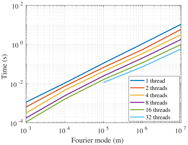
Figure 11: Evaluation time of the modal Green’s function plotted against $m$ with varying numbers of threads ($\beta_{-}=10^{-7},\kappa=10,000$). The calculation is performed in double precision. The evaluation times corresponding to 32 threads are not plotted for small $m$.

6 Conclusions and Generalizations

We have developed an algorithm which evaluates the modal Green’s function for the Helmholtz equation in $O(m)$ time, that is completely independent of both the wavenumber and the source-to-target distance. Furthermore, our algorithm is embarrassingly parallelizable. Our algorithm’s method can be readily extended to several associated problems in computational electromagnetics, described in Sections 6.1- 6.4.

6.1 An $O(1)$ Evaluator for Small Wavenumber ($\kappa\ll m$)

Recall that our algorithm is independent of the wavenumber because we integrate along Gustafsson’s contours, which are the steepest descent contours with respect to the spherical wave component (see Section 3.1). When the Fourier mode $m$ is larger than the scaled wavenumber $\kappa$, it is more efficient to integrate along a different contour. If instead, we choose the steepest descent contour on which $\exp{(im\phi)}$ does not oscillate, we arrive at an alternative algorithm whose cost is $O(\kappa)$ and independent of $m$ . When $\kappa$ is extremely small, this algorithm is essentially $O(1)$. The case where $\beta_{-}$ is small (i.e., when the source and target are close) is handled in an identical fashion to the method described in Section 4.2. Thus, this alternative algorithm’s cost is completely independent of both $m$ and $\beta_{-}$, and grows as $O(\kappa)$.

6.2 An $O(1)$ Evaluator of the Modal Green’s Functions for the Laplace Equation

The same method described in Section 6.1 can be applied to the case where $\kappa=0$ to yield an $O(1)$ evaluator of the modal Green’s function for the Laplace equation, whose cost is independent of $\beta_{-}$ (i.e., the cost is independent of the source-to-target distance).

6.3 Extension of the Algorithm to Complex $\kappa$

In this manuscript, we assumed $\kappa\in\mathbb{R}$ and $\kappa>0$, where $\kappa$ is the scaled wavenumber. When the scaled wavenumber $\kappa$ is complex (i.e., when the medium is attenuating), Gustafsson’s steepest descent contours are rotated in the complex plane. The same algorithm described in this manuscript applies in this case, with the only modification being a change in the geometry of the steepest descent contours and the locations of the intersection points of the contours with the Bernstein ellipse.

6.4 Extension to an $O(m)$ Evaluator for a Collection of Modal Green’s Functions, with Amortized Cost $O(1)$

This manuscript presents an algorithm for the evaluation of a single modal Green’s function for the Helmholtz Equation in $O(m)$ time, independent of $\beta_{-}$ and $\kappa$, where $\beta_{-}$ is the scaled minimum source-to-target distance and $\kappa$ is the scaled wavenumber. It is possible to use this algorithm to compute all of the modal Green’s functions $-M,-M+1,\dots,M-1,M$ in $O(M)$ time using the following method. In [17], Matviyenko presents a five-term recurrence relation for the modal Green’s functions for the Helmholtz equation. He observes that the recurrence relation is stable upwards for one range of Fourier modes and stable downwards for another range of modes. Furthermore, there exists a range of modes for which the recurrence is bi-unstable. Thus, a classical Miller-type algorithm cannot be applied. However, it was recently observed in [18] that if a recurrence relation is represented as a banded matrix, then the inverse power method can be used to find a solution, even when the stability behavior is mixed in the sense just described. We thus apply the inverse power method, as described in [18], to the resulting five-diagonal matrix corresponding to Matviyenko’s recurrence relation. In this fashion, we obtain all the eigenvectors corresponding to the zero eigenvalue; only one vector in this eigenspace corresponds to the vector of modal Green’s functions. We thus use the $O(m)$ evaluator of this manuscript to select the vector corresponding to the modal Green’s functions. The cost of performing the inverse-power method is $O(M)$, and the cost of the evaluation of the $M$th modal Green’s function is $O(M)$, meaning that all $M$ Fourier coefficients are obtained in $O(M)$ time.

References

- [1] Abdelmageed, Alaa K. “Efficient evaluation of modal Green’s function arising in EM scattering by bodies of revolution.” Pr. Electromag. Res. S. 27 (2000): 337–356.
- [2] Abramowitz, Milton and Irene A. Stegun. Handbook of Mathematical Functions. National Bureau of Standards, 1964.
- [3] Andreasen, M. “Scattering from bodies of revolution.” IEEE. T. Antenn. Propag. 13.2 (1965): 303–310.
- [4] Bremer, James. “An algorithm for the numerical evaluation of the associated Legendre functions that runs in time independent of degree and order.” J. Comput. Phys. 360 (2018): 15-38.
- [5] Bremer J., Z. Gimbutas, and V. Rokhlin. “A nonlinear optimization prcocedure for generalized Gaussian quadratures.” SIAM J. Sci. Comput. 32.4 (2010): 1761–1788.
- [6] Cheng, Hongwei, W.Y. Crutchfield, Z. Gimbutas, L.F. Greengard, J.F. Ethridge, J. Huang, V. Rokhlin, N. Yarvin, and J. Zhao. “A wideband fast multipole method for the Helmholtz equation in three dimensions.” J. Comput. Phys. 216.1 (2006): 300–325.
- [7] Cohl, H. and J. Tohline. “A Compact Cylindrical Green’s Function expansion for the Solution of Potential Problems.” Astrophys. J. 527.1 (1999): 86.
- [8] Conway, J. and H.S. Cohl. “Exact Fourier expansion in cylindrical coordinates for the three-dimensional Helmholtz Green function.” Z. Angew. Math. Phys. 61.3 (2010): 425–443.
- [9] Epstein, C., L. Greengard, and M. O’Neil. “A high-order wideband direct solver for electromagnetic scattering from bodies of revolution.” J. Comput. Phys. 387 (2019): 205–229.
- [10] Gedney, S. and R. Mittra. “The use of the FFT for the efficient solution of the problem of electromagnetic scattering by a obdy of revolution.” IEEE. T. Antenn. Propag. (1988): 92–95.
- [11] Gustafsson, Mats. “Accurate and efficient evaluation of modal Green’s functions.” J. of Electromagnet. Waves. 24.10 (2010): 1291–1301.
- [12] Helsing, J. and A. Holst. “Variants of an explicit kernel-split panel based Nystrom discretization scheme for Helmholtz boundary value problems.” Adv. Comput. Math. 41.3 (2015): 691–708.
- [13] Helsing, J. and A. Karlsson. “An explicit kernel-split panel-based Nystrom scheme for integral equations on axially symmetric surfaces.” J. Comput. Phys. 272 (2014): 686–703.
- [14] Lai, J. and M. O’Neil. “An FFT-accelerated direct solver for electromagnetic scaterring from penetrable axisymmetric objects.” J. Comput. Phys. 390 (2019): 152–174.
- [15] Liu, Y. and A. Barnett. “Efficient numerical solution of acoustic scattering from doubly-periodic arrays of axisymmetric objects.” J. Comput. Phys. 324 (2016): 226–245.
- [16] Mason, J. Chebyshev polynomials. CRC Press, 2002
- [17] Matviyenko, Gregory. “On the azimuthal Fourier components of the Green’s function for the Helmholtz equation in three dimensions.” J. Math. Phys. 36.9 (1995): 5159–5169.
- [18] Osipov, Andrei. “Evaluation of small elements of the eigenvectors of certain symmetric tridiagonal matrices with high relative accuracy.” Appl. Comput. Harmon. A. 43.2 (2017): 173–211
- [19] Trefethen, N. Approximation Theory and Practice. SIAM, 2019
- [20] Trefethen, N. Spectral methods in MATLAB. SIAM, 2000
- [21] Vaessen, Jean-Pierre A., and M. van Beurden. “Accurate and efficient computation of the modal Green’s function arising in the electric-field integral equations for a body of revolution.” IEEE T. Antenn. Propag. 60.7 (2012): 3294–3304.
- [22] Wang, Peng and G. Xiao. “A Note on the Singularity Extraction Technique in Solving Scattering Problems for Bodies of Revolution.” Asia Pacif. Microwave. (2010): 2146–2148.
- [23] Young, P., S. Hao, and P.G. Martinsson. “A high-order Nystrom discretization scheme for boundary integral equations defined on rotationally symmetric surfaces.” J. Comput. Phys. 40.1 (2014): 4142–4159.