Multiphoton resonance in a driven Kerr oscillator in presence of high–order nonlinearities

Abstract

We considered the multiphoton resonance in the periodically driven quantum oscillator with Kerr nonlinearity in the presence of weak high–order nonlinearities. Multiphoton resonance leads to the emergence of peaks and dips in the dependence of the stationary occupations of the stable states on detuning. We demonstrated that due to high–order nonlinearities, these peaks and dips acquire additional fine structure and split into several closely spaced ones. Quasiclassically, multiphoton resonance is treated as tunneling between the regions of the oscillator phase portrait, and the fine structure of the multiphoton resonance is a consequence of a special quasienergy dependence of the tunneling rate between different regions of the classical phase portrait. For different values of damping and high–order nonlinearity coefficients, we identified the domain of quasienergies where tunneling strongly influences the system kinetics. The corresponding tunneling term in the Fokker–Planck equation in quasienergy space was derived directly from the quantum master equation.

I Introduction

For decades, bistable and multistable systems attract researchers’ attention in many areas of physics. Bi– and multistability has been observed in many experimental setups including nonlinear–optical systems Azadpour and Bahari (2019), lasers Li et al. (2017), nanomechanical systems Pistolesi (2018), optical cavities interacting with ultracold atoms Gothe et al. (2019) or magnonic systems Wang et al. (2018). Recently, it became possible to observe bistability in systems operating with only a few excitation quanta Wang et al. (2019) Winkel et al. (2020) Muppalla et al. (2018). Such systems are promising candidates for the generation of squeezed states which are important for decreasing the noise–signal ratio in quantum measurements Maslova et al. (2019a). Moreover, they can be useful for the creation of entangled states which are crucial for applications in quantum information processing and safe quantum communications systems.

There exists a class of bistable systems that can be modeled as a nonlinear oscillator mode with Kerr nonlinearity driven by external resonant or parametric excitation. Such models describe a wide range of physical systems including the Fabry–Perot microcavities with nonlinear filling Gibbs et al. (1976), whispering gallery resonators, laser systems near threshold Bonifacio and Lugiato (1978), polariton microcavities, superconducting nonlinear resonators Wang et al. (2019) Winkel et al. (2020) Muppalla et al. (2018). On the classical level, the model of a driven nonlinear oscillator has two stable stationary states with different field amplitudes. With account for thermal noise, transitions between these states become possible. As the states 1 and 2 have different field amplitudes and intensities, they can be distinguished experimentally, for example, via a cross–Kerr induced shift in some probe mode. In the experiment, it is possible to observe random switching between the stable states Muppalla et al. (2018). Thus, it is of high interest to calculate the occupation probabilities of the stable states and the transition rates between them.

At small or moderate numbers of quanta circulating in the mode, quantum effects become important. Interestingly, when the number of quanta in the mode is several dozens, the quantum effects can be treated within the quasiclassical approximation, and it is still possible to use the classical concepts of the classical phase portrait and stable states. One of the most pronounced quantum effects is related with tunneling between different regions of the phase portrait of the classical oscillator. Tunneling transitions modify the occupation probabilities of the classical stable states and the transition rates, namely, they increase the occupation of the high–amplitude stable state and thus lead to enhanced excitation of the mode Maslova et al. (2019b) Anikin et al. (2019). In fact, tunneling between different regions of the phase portrait corresponds to the quasiclassical treatment of multiphoton transitions, namely, the excitation of the oscillator with simultaneous absorption of many external field quanta. A similar relation between multiphoton transitions and tunneling is known in the theory of multiphoton ionization of atoms Keldysh (1965).

In the model of a single oscillator mode with Kerr nonlinearity, tunneling and multiphoton transitions are especially important when the resonance condition is fulfilled. If no higher nonlinearities are present, this occurs when the detuning between the driving field and the oscillator mode is an integer or half–integer multiple of the Kerr frequency shift per quantum. This property follows from a special symmetry of the model Hamiltonian Anikin et al. (2019), and because of this, the eigenstates of the quantum Hamiltonian correspond to superpositions of quasiclassical states belonging to different regions of the phase portrait. Because of that, the dependence of the higher–amplitude and lower–amplitude states populations on detuning has pronounced peaks and drops at integer and half–integer detuning–nonlinearity ratio. However, in real systems, small higher–order nonlinearities always exist together with Kerr nonlinearity. It is of high interest to find out how their presence modifies the structure of multiphoton resonance.

In this manuscript, we consider the model of a quantum driven nonlinear oscillator which includes high–order nonlinearities as small corrections. Together with numerical simulations, we utilize the analytical approach of the Fokker–Planck equation in the quasienergy space with tunneling term obtained from the full quantum master equation. We demonstrate that in presence of high–order nonlinearities, the multiphoton resonance peaks in the occupations of the high–amplitude stable state split into several smaller ones with different widths and amplitudes. The magnitude of the splitting turns out to be proportional to high–order nonlinearity coefficients. In addition, we extend the analysis of previous works Maslova et al. (2019b) Anikin et al. (2019) to the case of finite damping having the order or being larger than tunneling and multiphoton splitting between the Hamiltonian eigenstates from different regions of the phase portrait.

II The model of a quantum driven nonlinear oscillator

We consider the model of a bistable driven system consisting of a resonant mode with Kerr–like nonlinearity Drummond and Walls (1980), Risken et al. (1987) and additional higher–order nonlinearities. The effective Hamiltonian of the system in the rotating–wave approximation reads

$$\begin{gathered}\hat{H}=-\Delta\hat{a}^{\dagger}\hat{a}+\frac{\alpha}{2}(\hat{a}^{\dagger}\hat{a})^{2}+\hat{V}+f(\hat{a}+\hat{a}^{\dagger}),\\ \hat{V}=\sum_{q=3}^{\infty}\alpha_{q}(a^{\dagger}a)^{q}\end{gathered}$$ (1)

The eigenstates of this effective Hamiltonian are the approximations of the exact Floquet states of the full time–dependent Hamiltonian, and the eigenvalues give the Floquet quasienergies. The parameter $\Delta$ is the detuning between the driving field and the resonant oscillator frequency, $\alpha$ is the Kerr coefficient, $\alpha_{q}$ is the $2q$–order nonlinearity coefficient, and $f$ is proportional to the amplitude of the driving field. In the following, we will mostly focus on the case of six–order nonlinearity, $q=3$.

The statistical properties of this model with account for weak interaction with the dissipative environment should be studied using the quantum master equation (QME): Haken (1965), Risken (1965), Graham and Haken (1970), Drummond and Walls (1980), Risken et al. (1987):

$$\partial_{t}\rho=i[\rho,\hat{H}]+\frac{\gamma}{2}\left(2\hat{a}\rho\hat{a}^{\dagger}-\rho a^{\dagger}a\right.\\ -a^{\dagger}a\rho\left.+2N[[a,\rho],a^{\dagger}]\right),$$ (2)

where $\gamma$ is the coupling strength with the dissipative environment, and $N$ is the number of thermal photons at the external field frequency.

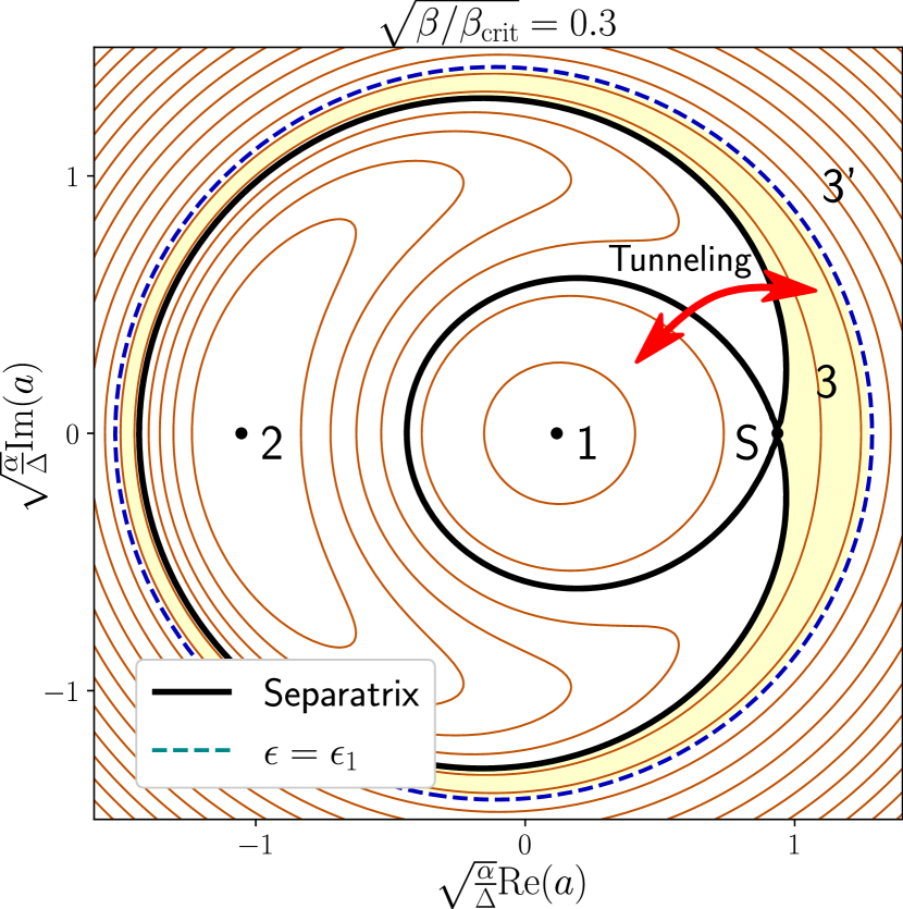
Figure 1: The classical phase portrait of the nonlinear oscillator with the Hamiltonian (1) for $f/f_{\mathrm{crit}}=0.3$, $\alpha_{3}=0$. The blue dashed line denotes a classical trajectory in region 3 having the same quasienergy $\epsilon_{1}$ as the stable state 1. From region 1, the system can exhibit tunneling transitions to the subregion of region 3 enclosed by the separatrix and this trajectory.

Both unitary dynamics governed by the system Hamiltonian (1) and dissipative dynamics described by QME (2) can be treated quasiclassically, if the Kerr nonlinearity is sufficiently small, $\Delta\gg\alpha$. While the exact unitary dynamics of the system are described by Heisenberg equations for operators $\hat{a},\hat{a}^{\dagger}$, one should replace these operators with the c–number field amplitudes $a$, $a^{*}$ in the system Hamiltonian (1) to obtain the classical limit. The time evolution of the classical field amplitudes $a$ and $a^{*}$ is the motion along the classical trajectories given by the contour lines of the classical Hamiltonian $H(a,a^{*})$. Also, according to Bohr–Sommerfeld rule, the eigenstates of the quantum Hamiltonian correspond to a discrete set of trajectories on the classical phase portrait in the quasiclassical limit. Importantly, the Bohr–Sommerfeld description does not take into account quantum tunneling which will be discussed below. For the dissipative dynamics in the same limit, the QME can be transformed into the classical 2D Vogel and Risken (1988) Maslova et al. (2007) or 1D Fokker–Planck equation Vogel and Risken (1990) Maslova et al. (2019b), which is equivalent to classical Langevin equations containing the Hamiltonian term, the damping term and the noise term. The quasiclassical approach demonstrates good agreement with the full quantum simulations even at moderate numbers of photons ($\sim 20$) Maslova et al. (2019b) circulating in the mode.

A prominent feature of the classical phase portrait is bistability, which is present for field values not exceeding the critical value $f_{\mathrm{crit}}=\sqrt{4\Delta^{3}/27\alpha}$ (at $\hat{V}=0$). In this case, there are two stable stationary states 1 and 2. In addition, there exists an unstable stationary state S and a self–intersecting trajectory (separatrix) passing through S. The separatrix divides the phase portrait into regions 1 and 2 containing the corresponding stable stationary states and the outer region 3 (see Fig. 1). The classical trajectories from region $2$ have quasienergies $\epsilon$ such as $\epsilon_{2}<\epsilon<\epsilon_{sep}$, where $\epsilon_{r}$ is the quasienergy of the classical stable state $r=1,2$, and $\epsilon_{sep}$ is the quasienergy of the unstable stationary state. For the trajectories from region 1, $\epsilon_{sep}<\epsilon<\epsilon_{1}$, and for the trajectories from region 3, $\epsilon>\epsilon_{sep}$. For additional details on the role of different quasienergy domains, please see Fig. 2 in Ref. Anikin et al. (2019). Also, the presence of small higher–order nonlinearities doesn’t change the qualitative structure of the classical phase portrait.

According to both the quasiclassical treatment of the model using the quasiclassical Fokker–Planck equation (FPE) Vogel and Risken (1990) and the full quantum treatment based on QME Drummond and Walls (1980) Risken et al. (1987), the system persists in the vicinity of the classical stable states 1 and 2 most of the time. Also, rare noise–induced transitions between the stable states occur. Thus, the probabilities to find the system close to the stable states 1 and 2, $\bm{P}_{1}$ and $\bm{P}_{2}$, can be identified with the probabilities to find the system in regions 1 and 2 of the classical phase portrait. In the classical limit, they can be found from the stationary solutions of the FPE as the integrals of the probability density over the corresponding domain of quasienergies. Beyond the applicability of FPE, they can be obtained from the stationary solutions of the QME.

III Tunneling between the regions of the classical phase portrait

For each classical trajectory in region 1, there exists a trajectory with the same value of quasienergy in region 3 (see Fig. 1). Quantum mechanics allow the system to undergo a tunneling transition between two such classical trajectories, so the Bohr–Sommerfeld quasiclassical description of the eigenstates of the quantum Hamiltonian should be modified with account for tunneling. Actually, the real Hamiltonian eigenstates can be considered as quantum superpositions of the trajectories belonging to different regions of the phase portrait. However, the tunneling amplitude is exponentially small in comparison with the spacing between the quasienergy levels within each region. Because of that, the trajectories form superpositions only when a certain resonance condition for the system parameters is fulfilled. In absence of high–order nonlinearities, it was shown Anikin et al. (2019) that this happens when the detuning $\Delta$ is an integer or half–integer multiple of $\alpha$ independently of $f$. This manifests as the anticrossings of the Hamiltonian quasienergy levels dependence on $\Delta$ at the constant driving field. (see the inset on Fig. 2). Moreover, a prominent feature of the model without high–order nonlinearities is that the anticrossings of many pairs of levels occur simultaneously. This is a consequence of a special symmetry of the system Hamiltonian, namely, the symmetry of the perturbation theory series for the system quasienergies $\epsilon_{n}$ in $f$. Also, it can be seen from the results of numerical diagonalization, which are shown in Fig. 2.

Since the true eigenstates of the Hamiltonian can be superpositions of trajectories from regions 1 and 3, it is convenient to use the basis of states which are not the eigenstates of the quantum Hamiltonian but correspond to a discrete set of classical trajectories lying entirely in one of the regions of the phase portrait. In such a basis, Hamiltonian is not diagonal, and matrix elements corresponding to tunneling transitions between different regions of the classical phase space are present. Also, when $2\Delta/\alpha$ is close to an integer, the quasienergy levels group into pairs with very close values of quasienergy, and the tunneling matrix element can be retained only between the states within each pair. Thus, the Hamiltonian in the suggested basis reads

$$\hat{H}=\sum_{n}\begin{pmatrix}|n,1\rangle&|n,3\rangle\end{pmatrix}\begin{pmatrix}\epsilon_{n1}&t_{n}\\ t_{n}&\epsilon_{n3}\end{pmatrix}\begin{pmatrix}|n,1\rangle\\ |n,3\rangle\end{pmatrix}\\ +\sum_{n}\epsilon_{n2}|n,2\rangle\langle n,2|+\sum_{n}\epsilon_{n3^{\prime}}|n,3^{\prime}\rangle\langle n,3^{\prime}|$$ (3)

Here $|n,2\rangle$ are the states from region 2, and $|n,3^{\prime}\rangle$ are the states from region 3 with quasienergies higher than the states from region 1. These states are not affected by tunneling. Then, the states $|n,1\rangle$ and $|n,3\rangle$ form the pairs of the basis states from regions 1 and 3 with close values of mean quasienergy $\epsilon_{n1}$ and $\epsilon_{n3}$. It is necessary to take the amplitude of tunneling $t_{n}$ between them, which can be estimated as Maslova et al. (2019b)

$$\begin{gathered}t_{n}\sim\Delta e^{-S_{\mathrm{tunn}}(\epsilon_{n})},\\ S_{\mathrm{tunn}}=\frac{\Delta}{\alpha}\int_{q_{1}}^{q_{2}}\operatorname{acosh}\left\{\frac{\frac{\alpha\epsilon}{\Delta^{2}}+\frac{s^{2}}{2}-\frac{s^{4}}{8}}{s\sqrt{2\alpha f^{2}/\Delta^{3}}}\right\}s\,ds,\end{gathered}$$ (4)

In the integral in the expression for tunneling amplitude, $q_{1}$ and $q_{2}$ are two branching points of the $\operatorname{acosh}$ function.

The anticrossings of the quasienergy levels affect the statistical and kinetic properties of the model because of enhanced tunneling between the regions of the phase space. It was shown Maslova et al. (2019b) that tunneling decreases the population of the stable state 1 and increases the population of the stable state 2 due to the presence of an additional escape channel from classical region 1. Thus, each anticrossing decreases the population of the stable state 1 and increases the population of the stable state 2 and the field intensity in the mode.

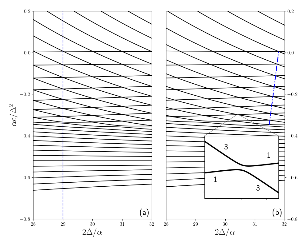
Figure 2: The eigenvalues of the Hamiltonian (1) obtained via exact numerical diagonalization are shown for different ratios between the detuning $\Delta$ and nonlinearity $\alpha$ at $f/f_{\mathrm{crit}}=0.1$ and (a) $\alpha_{3}=0$, (b) $\alpha_{3}/\alpha=0.005$. In absence of high–order nonlinearity, all anticrossings occur at integer values of $m$ and lie on a single vertical line (see the blue dashed vertical line in (a)). This is not the case in presence of six–order nonlinearity, when the anticrossings of quasienergy levels occur at different values of $2\Delta/\alpha$. On the inset, zoomed region of anticrossing between the levels from classical regions 1 and 3 is shown.

In presence of nonvanishing $\hat{V}$, the anticrossings of different pairs of quasienergy levels occur at close but different values of detuning (see Fig. 2b). This can be explained by considering $\hat{V}$ as a small perturbation. It is convenient in the basis introduced above because the averages of $\hat{V}$ over the basis states can be calculated as the c–function averages over classical phase trajectories.

Let us consider a pair of levels $n_{1}$ and $n_{3}$ which exhibit anticrossing at the detuning value $\Delta_{0}=m_{0}\alpha/2$, $m_{0}\in\mathbb{Z}$, when $\hat{V}=0$. This means that $\epsilon_{n1}=\epsilon_{n3}$ at this value of $\Delta$. When high–order nonlinearities are present, $\epsilon_{n1}$ and $\epsilon_{n3}$ acquire first–order corrections, and the anticrossing of the levels occurs at some $\Delta=\Delta_{0}+\delta\Delta$. By treating $\delta\Delta$ as a perturbation together with $\hat{V}$, one can get the expression for the quasienergy differences

$$\epsilon_{n1}-\epsilon_{n3}=\delta\Delta\left((a^{\dagger}a)^{11}_{nn}-(a^{\dagger}a)^{33}_{nn}\right)+V^{11}_{nn}-V^{33}_{nn},$$ (5)

where $\langle n,r|\hat{O}|n^{\prime},r^{\prime}\rangle\equiv O^{rr^{\prime}}_{nn^{\prime}}$ for any operator $\hat{O}$. The new anticrossing position follows from the equality $\epsilon_{n1}(\Delta_{0}+\delta\Delta_{n},\alpha_{q})=\epsilon_{n3}(\Delta_{0}+\delta\Delta_{n},\alpha_{q})$:

$$\delta\Delta_{n}=\frac{V_{nn}^{33}-V_{nn}^{11}}{(\hat{a}^{\dagger}\hat{a})_{nn}^{33}-(\hat{a}^{\dagger}\hat{a})_{nn}^{11}}$$ (6)

When the shifts of the anticrossing positions are considerably smaller than $\alpha/2$, the anticrossings are located near the integer values of $2\Delta/\alpha$. The number of anticrossings near each integer $m=\frac{2\Delta}{\alpha}$, is proportional to $m$, and their offsets from integer values are of order $\alpha_{3}m^{2}$. Basing on an accurate analysis of the quantum master equation, we will show below that level anticrossings give rise to a set of peaks near integer values of $2\Delta/\alpha$ in the high–amplitude stable state occupation.

IV Multiphoton resonance and the populations of the stationary states

To analyze the effect of tunneling on the stationary density matrix and the populations of the classical stable stationary states, let us consider the master equation (2) in the basis of states $|n,1\rangle$, $|n,2\rangle$, $|n,3\rangle$ and $|n,3^{\prime}\rangle$ introduced in Section III (see also Eq. 3). By employing the diagonal approximation in this basis and performing the gradient expansion, the classical FPE in quasienergy representation can be obtained in the limit of large $2\Delta/\alpha$, constant ratio $\alpha(N+1/2)/\Delta$ and small $\gamma/\Delta$ Maslova et al. (2019b). Tunneling between the regions of the phase portrait is mediated by the nondiagonal elements of the density matrix and lies beyond this approximation. However, it is possible to retain only the density matrix elements $\rho_{nn^{\prime}}^{rr^{\prime}}$ with $n=n^{\prime}$ (denoted hereafter as $\rho_{n}^{rr^{\prime}}$), because $\rho_{nn^{\prime}}^{rr^{\prime}}$ are proportional to $\gamma/(\epsilon_{n1}-\epsilon_{n^{\prime}3})$ and can be neglected as long as $\gamma$ is small in comparison to the quasienergy spacing within each region of the phase portrait. Also, the matrix elements of the annihilation operator $\hat{a}$ between the states lying in different regions of the phase portrait, $r\neq r^{\prime}$, are exponentially small and can be neglected. Under such approximations, the master equation for regions 1 and 3 takes the form

$$\partial_{t}\rho_{n}^{rr}=\pm it_{n}(\rho_{n}^{13}-\rho_{n}^{31})-\gamma(N+1)\left((a^{\dagger}a)_{nn}^{rr}\rho_{n}^{rr}-\sum_{n^{\prime}}a_{nn^{\prime}}^{rr}(a_{nn^{\prime}}^{rr})^{*}\rho_{n^{\prime}}^{rr}\right)\\ -\gamma N\left((aa^{\dagger})_{nn}^{rr}\rho_{n}^{rr}-\sum_{n^{\prime}}(a_{n^{\prime}n}^{rr})^{*}a_{n^{\prime}n}^{rr}\rho_{n^{\prime}}^{rr}\right),\quad r=1,3$$ (7)

$$\partial_{t}\rho_{n}^{13}=-i(\epsilon_{n1}-\epsilon_{n3})\rho_{n}^{13}+it_{n}(\rho_{n}^{11}-\rho_{n}^{33})\\ -\frac{\gamma}{2}(N+1)\left((a^{\dagger}a)_{nn}^{11}\rho_{n}^{13}+(a^{\dagger}a)_{nn}^{33}\rho_{n}^{13}-\sum_{n^{\prime}}2a_{nn^{\prime}}^{11}(a_{nn^{\prime}}^{33})^{*}\rho_{n^{\prime}}^{13}\right)\\ -\frac{\gamma N}{2}\left((aa^{\dagger})_{nn}^{11}\rho_{n}^{13}+(aa^{\dagger})_{nn}^{33}\rho_{n}^{13}-\sum_{n^{\prime}}2(a_{n^{\prime}n}^{11})^{*}a_{n^{\prime}n}^{33}\rho_{n^{\prime}}^{13}\right)$$ (8)

The system of equations (7) and (8) can be transformed into continuous form by considering the density matrix elements $\rho_{n}^{11}$, $\rho_{n}^{33}$ as continuous functions $P_{1}$, $P_{3}$ of $n$ and performing the gradient expansion like in Maslova et al. (2019b). For our purposes, it is more convenient to use the quasienergy $\epsilon(n)=(\epsilon_{n1}+\epsilon_{n3})/2$ as an independent continuous variable. Also, in the stationary case, it is possible to express the nondiagonal density matrix elements $\rho_{n}^{13}$ from (8) and to substitute them into (7). The resulting equations for $P_{r}(\epsilon)$, $r=1,3$ in the domain of quasienergies $\epsilon_{\mathrm{sep}}<\epsilon<\epsilon_{1}$ read

$$\frac{1}{T_{r}(\epsilon)}\frac{\partial}{\partial\epsilon}\left[\gamma K_{r}P_{r}+QD_{r}\frac{\partial P_{r}}{\partial\epsilon}\right]\pm\lambda_{T}(P_{3}-P_{1})=0$$ (9)

where $T_{r}(\epsilon)$ is the period of motion along the classical trajectories, $K_{r}(\epsilon)$, $D_{r}(\epsilon)$ are the drift and diffusion coefficients in quasienergy space in each region of the classical phase portrait, $Q=\gamma(N+1/2)$ is the noise intensity, and $\lambda_{T}(\epsilon)$ is a coefficient which can be interpreted as the rate of tunneling transitions between the regions of the classical phase portrait. The term with $\lambda_{T}(\epsilon)$ arises because of the presence of nondiagonal elements of the density matrix, and the particular form of $\lambda_{T}(\epsilon)$ will be derived directly from the master equations (7) and (8). It turns out that $\lambda_{T}(\epsilon)$ has a nontrivial dependence on $\epsilon$, $\Delta$, the coefficients $\alpha_{q}$ in $\hat{V}$ and $\gamma$. Below, we will show that the tunneling term $\lambda_{T}(P_{3}-P_{1})$ strongly changes the stationary distribution function and the populations of the stationary states. By examining $\lambda_{T}(\epsilon)$, it is possible to explain the structure of resonant peaks in the occupation of the classical stationary state 2 in presence of high–order nonlinearities and finite damping.

Before proceeding to the derivation of $\lambda_{T}(\epsilon)$, let us give the qualitative analysis of the role of tunneling between different pairs of almost–degenerate states $|n,1\rangle$ and $|n,3\rangle$. Tunneling between these states has different importance for different $n$: when

$$t_{n}\gtrsim|\epsilon_{n1}-\epsilon_{n3}|,$$ (10)

tunneling is strong and leads to the hybridization of the states $|n,1\rangle$ and $|n,3\rangle$. In the opposite case, $t_{n}\ll|\epsilon_{n1}-\epsilon_{n3}|$, tunneling can be neglected. The inequality $t_{n}\gg|\epsilon_{n1}-\epsilon_{n3}|$ holds in two different cases. First, it is always satisfied for such $n$ that $t_{n}\gg\delta\Delta,\alpha_{3}$ because $|\epsilon_{n1}-\epsilon_{n3}|$ is of order $\delta\Delta$, $\alpha_{3}$, see Eq. (5). There can be many pairs of states $|n,1\rangle$ and $|n,3\rangle$ for which $t_{n}\gg\delta\Delta,\alpha_{3}$. Because of the exponential decay of $t_{n}$ away from the separatrix, they lie in the domain of quasienergies $\epsilon_{\mathrm{sep}}<\epsilon<\epsilon_{\mathrm{crit}}$, where $\epsilon_{\mathrm{crit}}$ is is a new parameter depending on $\delta\Delta$, $\alpha_{3}$ and $\gamma$ which we call critical quasienergy. From Eq. 10, it follows that $\epsilon_{\mathrm{crit}}$ is a minimal value among the roots of the two equations $\delta\epsilon_{13}(\epsilon)=\pm t(\epsilon)$, where $t(\epsilon)$ and $\delta_{13}(\epsilon)$ are the continuous limits of $t_{n}$ and $\epsilon_{n1}-\epsilon_{n3}$ taken as functions of the quasienergy $\epsilon$ (see Fig. 3). Second, even in the case $t_{n}\ll\delta\Delta,\alpha_{3}$, the inequality (10) still can be satisfied for a single pair of the states $|n,1\rangle$ and $|n,3\rangle$ for some $n=n_{\mathrm{res}}$ if $\epsilon_{n1}-\epsilon_{n3}$ passes near zero at $n_{\mathrm{res}}$. This is possible because two terms in Eq. (5) may have different signs, and physically this can be interpreted as resonant tunneling through a single pair of almost–degenerate states. However, such a pair of states exists only when higher–order nonlinearities are present.

The steps to derive (9) from (7) and (8) assuming that $\partial_{t}\hat{\rho}=0$ are as follows. First, one should express the nondiagonal density matrix elements $\rho^{13}_{n}$ and $\rho^{31}_{n}$ through $\rho^{11}_{n}$ and $\rho^{33}_{n}$ using Eq. (7). Then, they should be substituted into (7), and the continuous limit should be obtained. After the calculation presented in Appendix A, one gets the tunneling rate as

$$\lambda_{T}(\epsilon)=\begin{cases}\displaystyle\frac{\gamma_{13}(\epsilon)t^{2}(\epsilon)}{\delta\epsilon_{13}(\epsilon)^{2}+\frac{\gamma_{13}^{2}(\epsilon)}{4}},&\epsilon_{\mathrm{sep}}<\epsilon<\epsilon_{\mathrm{crit}}\\ \displaystyle\frac{\tilde{\gamma}^{13}_{n_{\mathrm{res}}}t^{2}(\epsilon_{\mathrm{res}})}{\delta\epsilon_{13\mathrm{res}}^{2}+\frac{(\tilde{\gamma}^{13}_{n_{\mathrm{res}}})^{2}}{4}}\frac{\delta(\epsilon-\epsilon_{\mathrm{res}})}{T(\epsilon)},&\epsilon_{\mathrm{crit}}<\epsilon<\epsilon_{1}\\ \end{cases},$$ (11)

where $t(\epsilon)$ and $\delta_{13}(\epsilon)$ are the continuous limits of $t_{n}$ and $\epsilon_{n1}-\epsilon_{n3}$ taken as functions of the quasienergy $\epsilon$, and

$$\gamma_{n13}=\gamma\left((a^{\dagger}a)_{nn}^{11}+(a^{\dagger}a)_{nn}^{33}-2\sum_{n^{\prime}}a_{nn^{\prime}}^{11}(a^{33}_{nn^{\prime}})^{*}\right)$$ (12)

$$\tilde{\gamma}_{n13}=\frac{\gamma}{2}\left((a^{\dagger}a)_{nn}^{11}+(a^{\dagger}a)_{nn}^{33}-2a_{nn}^{11}(a_{nn}^{33})^{*}\right)$$ (13)

The delta–function term in (11) exists only when higher–order nonlinearities are present. Below, we will show that it leads to emergence of the fine structure of the multiphoton resonance peak in $\bm{P}_{2}$, namely, several additional narrow side peaks.

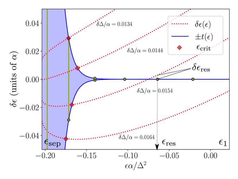
Figure 3: For different detunings $\delta\Delta$, the behavior of $\epsilon_{\mathrm{crit}}$ and $\epsilon_{\mathrm{res}}$ is demonstrated by comparing two sides of the inequality (10). The red dashed lines depict $\delta\epsilon_{13}(\epsilon)$ and blue solid lines depict the tunneling amplitude $t(\epsilon)$ for $\alpha_{3}/\alpha=10^{-5}$.

After we described the behavior of $\lambda_{T}(\epsilon)$, let us analyze the stationary distribution $P_{r}(\epsilon)$ over quasienergies. In each of the domains $\epsilon_{\mathrm{sep}}<\epsilon<\epsilon_{\mathrm{crit}}$, $\epsilon_{\mathrm{crit}}<\epsilon<\epsilon_{\mathrm{res}}$, $\epsilon_{\mathrm{res}}<\epsilon<\epsilon_{1}$, different analytical expressions for the stationary distribution function can be obtained. Due to strong tunneling in the domain $\epsilon_{\mathrm{sep}}<\epsilon<\epsilon_{\mathrm{crit}}$, the probability distributions in regions 1 and 3 become almost equal, $P_{1}\approx P_{3}$. By considering the sum of the equations (9) for $P_{1}$ and $P_{3}$, one can obtain a single first–order differential equation for distribution functions $P_{1,3}$. The details of the calculation are given in the Appendix A. The resulting distribution function in the domain $\epsilon_{\mathrm{sep}}<\epsilon<\epsilon_{\mathrm{crit}}$ turns out to decay exponentially away from the separatrix. This in contrast with the case of the purely classical oscillator, for which the distribution function $P_{1}(\epsilon)$ grows exponentially away from the separatrix. In the domain $\epsilon_{\mathrm{crit}}<\epsilon<\epsilon_{1}$, tunneling transitions occur only for the quasienergy $\epsilon\approx\epsilon_{\mathrm{res}}$ due to a delta–function peak in $\lambda_{T}(\epsilon)$. Because of that, the stationary distributions in the domain $\epsilon_{\mathrm{crit}}<\epsilon<\epsilon_{\mathrm{res}}$ are the solutions of (9) with nonzero probability flow. The flow can be obtained from boundary conditions at $\epsilon_{\mathrm{res}}$ obtained by integrating (9) in the vicinity of $\epsilon_{res}$. Finally, for $\epsilon>\epsilon_{\mathrm{res}}$, the stationary distributions in regions 1 and 3 coincide with the solutions of (9) without tunneling term and with zero probability flow. The example of such an analytical solution of the FPE is shown in Fig. 4, and the detailed calculation is given in Appendix B.

The solution of the FPE demonstrates that tunneling through the domain $\epsilon_{\mathrm{sep}}<\epsilon<\epsilon_{\mathrm{crit}}$ and through the resonant pair increase the population of the stable state 2. Now let us analyze how the obtained solutions depend on $\Delta$, $\gamma$ and $\alpha_{3}$.

Let us analyze the behavior of $\epsilon_{\mathrm{crit}}$. Analyzing its definition as the minimal root of $\delta\epsilon_{13}(\epsilon)=\pm t(\epsilon)$, one deduces that $\epsilon_{\mathrm{crit}}$ has a sharp peak at some value of $\delta\Delta$ and decays to $\epsilon_{\mathrm{sep}}$ away from it. The more $\epsilon_{\mathrm{crit}}$ is, the more pairs of states $|n,1\rangle$ and $|n,3\rangle$ with quasienergies $\epsilon_{\mathrm{sep}}<\epsilon_{n}<\epsilon_{\mathrm{crit}}$ strongly contribute to tunneling between the regions of the classical phase portrait. Thus, the maximum in $\epsilon_{\mathrm{crit}}$ results in a peak of the probability $\bm{P}_{2}$ to find the system in the classical region 2.

In addition, the delta–function term in $\lambda_{T}(\epsilon)$ is present when the condition (10) is satisfied for $n_{\mathrm{res}}$ such as $t_{n_{\mathrm{res}}}\ll\delta\Delta,\alpha_{3}$. As discussed in section III, the condition $\epsilon_{n_{\mathrm{res}}1}=\epsilon_{n_{\mathrm{res}}3}$ is the condition of level anticrossing which is satisfied at $\delta\Delta=\delta\Delta_{n_{res}}$ defined by Eq. (6). So, at each $\delta\Delta=\delta\Delta_{n}$ being much larger than the tunneling amplitude $t_{n_{\mathrm{res}}}$, there is also a narrow peak in $\bm{P}_{2}$.

Thus, the peaks in the population of the high–amplitude stable state dependence on $\Delta$ acquire fine structure due to high–order nonlinearity. Namely, a sequence of narrow side peaks with the spacing of order $\alpha_{3}\Delta/\alpha$ arise near the main resonance, and the number of these peaks is $\sim\Delta/\alpha$. This qualitative picture holds until the width of the whole sequence of peaks ($\sim\alpha_{3}\Delta^{2}\alpha^{2}$) becomes comparable with $\alpha$ and different sequences of peaks start to overlap.

These predictions are in good correspondence with the results of numerical solution of the full quantum master equation (2), see Fig. 5 and Fig. 6. In Fig. 5, $\bm{P}_{2}$ is shown as a function of $\Delta$ together with the differences of the quasienergies of the Hamiltonian eigenstates which exhibit anticrossings. Each peak in the probability $\bm{P}_{2}$ of the stable state 2 occupation is located at the value of $\Delta$ corresponding to a minimal difference between the eigenstates quasienergies.

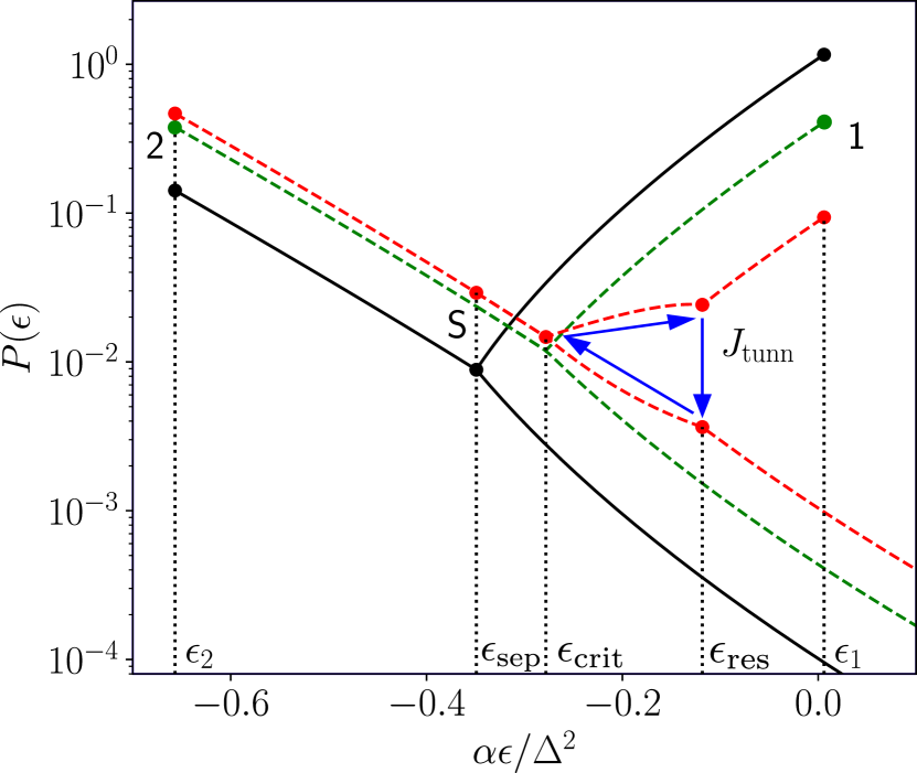
Figure 4: For $f/f_{\mathrm{crit}}=0.2$, $\alpha Q/(\Delta\gamma)=0.1$, the theoretically predicted stationary probability distribution function of a nonlinear oscillator with six–order nonlinearity near multiphoton resonance is shown by a red dashed line when the tunneling domain $\epsilon_{\mathrm{sep}}<\epsilon<\epsilon_{\mathrm{crit}}$ exists together with a single pair of degenerate states at $\epsilon=\epsilon_{\mathrm{res}}$. For comparison, the probability distribution function is also shown by a green line when the resonant pair of states does not exist, and the distribution function of ththee purely classical oscillator is shown by a black solid line.

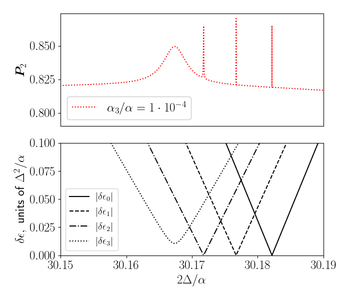
Figure 5: The dependence of the occupation of the higher–amplitude stable state of the quantum driven nonlinear oscillator with six–order nonlinearity on $2\Delta/\alpha$ is shown in (a) for $f/f_{\mathrm{crit}}=0.4$, $\alpha_{3}/\alpha^{2}=1\cdot 10^{-4}$. In (b), the differences between the pairs of anticrossing quasienergy levels are shown. Each peak in $\bm{P}_{2}(\Delta)$ corresponds to an anticrossing of two quasienergy levels.

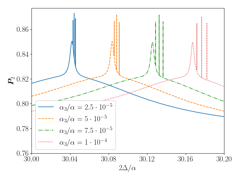
Figure 6: For the quantum driven nonlinear oscillator with six–order nonlinearity, the dependence of the probability $\bm{P}_{2}$ to find the system in the classical region 2 on $\Delta$ is shown in the limit of $\gamma\to 0$ for $f/f_{\mathrm{crit}}=0.4$, $N=3$, and for different values of $\alpha_{3}/\alpha$. The position of each of the peaks corresponding to multiphoton resonance depends linearly on $\alpha_{3}/\alpha$, and at $\alpha_{3}/\alpha=0$ the peaks merge.

In addition, let us analyze the effect of finite damping on the described fine structure of the multiphoton resonance. This can be done simply by analyzing the equations (11) because they are derived from the master equation (7), (8) which already accounts for the effect of damping and the nondiagonal elements of the density matrix. First, the role of the delta–peak in (11) corresponding to the resonance between the $n_{\mathrm{res}}$–th pair of levels depends on the ratio between $t_{n_{\mathrm{res}}}$ and the corresponding decay constant $\tilde{\gamma}_{n13}$. Thus, at increasing $\gamma$, the side peaks disappear in the order of increasing $t(\epsilon_{n})$. No side peaks are left when $\gamma$ reaches the value of $t(\epsilon_{\mathrm{crit}}^{\mathrm{max}})$, where $\epsilon_{\mathrm{crit}}^{\mathrm{max}}$ is the maximum value of $\epsilon_{\mathrm{crit}}$ depending on $\delta\Delta$. At larger $\gamma$, the depth of the main peak also becomes $\gamma$–dependent because $\lambda_{T}(\epsilon)$ can be neglected for the quasienergies $t(\epsilon)\ll\gamma$.

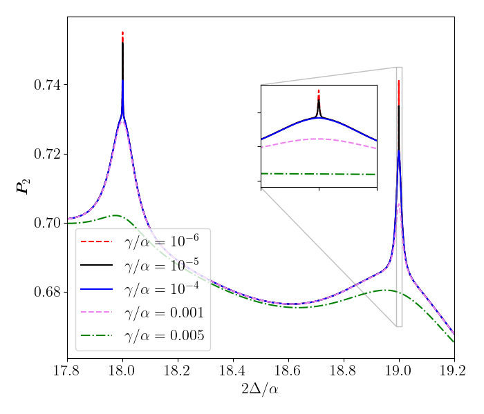
Figure 7: For the quantum driven nonlinear oscillator with $\alpha_{3}=0$, the probability to be in the classical region 2 is shown as a function of $2\Delta/\alpha$ for different values of $\gamma$. At $\gamma=0$, there are sharp peaks at integer corresponding to multiphoton resonance. At increasing $\gamma$, the drops become smoother.

V Conclusions

In conclusion, we analyzed the effect of multiphoton resonance on the populations of the stable states of the quantum nonlinear oscillator in resonant driving field. By including the tunneling term into one–dimensional quasiclassical Fokker–Planck equation in quasienergy space, we demonstrated that the mean–field intensity exhibits peaks near the values of external field frequency corresponding to multiphoton resonance. These peaks were associated with the anticrossings of the quasienergy levels of the oscillator. Also, we considered the effect of the higher–order nonlinearities on the structure of these peaks. We showed that due to high–order nonlinearities, the intensity peaks corresponding to multiphoton resonance acquire additional fine structure and split into several closely spaced side peaks which could be observed for modes with ultra–high quality factor. The reason for that splitting is that high–order nonlinearities break the special symmetry specific for purely Kerr nonlinearity. Such structure of the multiphoton resonance intensity peak is explained by a special dependence of the tunneling rate on quasienergy which is derived from the full master equation.

Appendix A The continuous limit of the quantum master equation

In this Appendix, we derive the Fokker–Planck equation with tunneling term (9) from the approximate form of the quantum master equation (7), (8). The first step is to express $\rho_{n}^{13}$ through $\rho_{n}^{11}$ and $\rho_{n}^{33}$ using the Eq. (8). This should be done differently in the quasienergy domains $\epsilon_{\mathrm{sep}}<\epsilon<\epsilon_{\mathrm{crit}}$ and $\epsilon_{\mathrm{crit}}<\epsilon<\epsilon_{1}$.

To express $\rho_{n}^{13}$ in the domain $\epsilon_{\mathrm{sep}}<\epsilon<\epsilon_{\mathrm{crit}}$, one should perform the gradient expansion of the $\gamma$–dependent term in (8). It results in the following expression:

$$\rho_{n13}=\frac{t_{n}(\rho_{n}^{11}-\rho_{n}^{33})}{\epsilon_{n1}-\epsilon_{n3}-\frac{i\gamma_{n13}}{2}},$$ (14)

where

$$\gamma_{n13}=\gamma\left((a^{\dagger}a)_{nn}^{11}+(a^{\dagger}a)_{nn}^{33}-2\sum_{n^{\prime}}a_{nn^{\prime}}^{11}(a_{nn^{\prime}}^{33})^{*}\right)$$ (15)

In the domain $\epsilon_{\mathrm{crit}}<\epsilon<\epsilon_{1}$, the only nondiagonal element of the density matrix which should be taken into account is the element corresponding to the transition between the pair of resonant states, $\rho_{n_{\mathrm{res}}}^{13}$, and all other can be neglected. Because of that, $\rho_{n_{res}}^{13}$ can be immediately expressed from (8):

$$\rho_{n_{res}}^{13}=\frac{t_{n_{res}}(\rho_{n_{res}}^{11}-\rho_{n_{res}}^{33})}{\epsilon_{n_{res}1}-\epsilon_{n_{res}3}-\frac{i\tilde{\gamma}_{13}}{2}},$$ (16)

$$\tilde{\gamma}_{13}=\frac{\gamma}{2}\left((a^{\dagger}a)_{n_{res}n_{res}}^{11}+(a^{\dagger}a)_{n_{res}n_{res}}^{33}\right.\\ -\left.2a_{n_{res}n_{res}}^{11}(a_{n_{res}n_{res}}^{33})^{*}\right).$$ (17)

Then, $\rho_{n}^{13}$ from (14), (16) should be substituted in (7). They are present in the term $\pm it_{n}(\rho^{13}_{nn}-\rho^{31}_{nn})$.

Now, let us focus on the part containing the diagonal elements of the density matrix $\rho^{11}_{n}$ and $\rho^{33}_{n}$. To transform the quantum master equation in the continuous form, one should consider $\rho^{11}_{n}$ and $\rho^{33}_{n}$ as the continuous functions $P^{r}(n)$ of the index $n$. Then, in the equation for each matrix element $\rho^{rr}_{n}$, the gradient expansion of $\rho^{rr}_{n^{\prime}}\equiv P^{r}(n^{\prime})$ should be performed: $P^{r}(n^{\prime})\approx P^{r}(n)+(n-n^{\prime})\frac{\partial P^{r}}{\partial n}+\frac{1}{2}(n-n^{\prime})^{2}\frac{\partial^{2}P^{r}}{\partial n^{2}}+\dots$. After truncating the expansion up to the second order, one gets the Fokker–Planck equation with the tunneling term (9). The resulting drift and diffusion coefficients $K_{r}(\epsilon)$, $D_{r}(\epsilon)$ and the period $T_{r}(\epsilon)$ can be found as the contour integrals over classical trajectories of the nonlinear oscillator:

$$\begin{gathered}K_{r}(\epsilon)=\frac{i}{2}\oint a\,da^{*}-a^{*}\,da,\\ D_{r}(\epsilon)=\frac{i}{2}\oint\frac{\partial H}{\partial a}da-\frac{\partial H}{\partial a^{*}}da^{*},\\ T_{r}(\epsilon)=\int da^{*}da\,\delta(\epsilon-H(a^{*},a)).\\ \end{gathered}$$ (18)

Appendix B The stationary solution of the Fokker–Planck equation with a tunneling term

In this Appendix, we present the accurate calculation of the stationary distribution function which follows from Eq. (9), where the tunneling rate $\lambda_{T}(\epsilon)$ is given by Eq. (11). First of all, let us consider the domain $\epsilon_{sep}<\epsilon<\epsilon_{crit}$. In this domain, tunneling leads to the equilibration of distribution functions in regions 1 and 3. So, $P_{1}(\epsilon)\approx P_{3}(\epsilon)$, and the equation for stationary distribution can be obtained by taking the sum of the equations for $P_{1}$ and $P_{3}$:

$$\left[\gamma(K_{1}+K_{3})P_{1,3}+Q(D_{1}+D_{3})\frac{\partial P_{1,3}}{\partial\epsilon}\right]=0,$$ (19)

Then, let us consider the domain $\epsilon_{crit}<\epsilon<\epsilon_{1}$. Due to the presence of the delta–like peak in $\lambda_{T}(\epsilon)$ at $\epsilon_{res}$, the stationary distribution function has nonzero probability flow $J$ at quasienergies $\epsilon_{crit}<\epsilon<\epsilon_{res}$ as presented in Fig. 4 Thus, the distribution functions $P_{1}$ and $P_{3}$ obey the equations

$$\gamma\left[\gamma K_{1,3}P_{1,3}+QD_{1,3}\frac{\partial P_{1,3}}{\partial\epsilon}\right]=\begin{cases}\mp J,&\epsilon_{crit}<\epsilon<\epsilon_{res}\\ 0,&\epsilon>\epsilon_{res}\end{cases}.$$ (20)

The flow $J$ is defined from the boundary condition $J=\lambda_{T}(\epsilon_{res})(P_{1}(\epsilon_{res})-P_{3}(\epsilon_{res}))$ which can be obtained by integrating Eq. (9) in the vicinity of $\epsilon_{res}$. As a result, the stationary distribution function determined from the solutions of (19) and (20) read

$$\begin{gathered}P_{r}(\epsilon)=\begin{cases}P(\epsilon_{sep})\exp{\left\{-\frac{\gamma}{Q}\int_{\epsilon_{\mathrm{sep}}}^{\epsilon}\frac{K_{1}(\epsilon^{\prime})+K_{3}(\epsilon^{\prime})}{D_{1}(\epsilon^{\prime})+D_{3}(\epsilon^{\prime})}d\epsilon^{\prime}\right\}}&\epsilon_{\mathrm{sep}}<\epsilon\leq\epsilon_{crit}\\ P(\epsilon_{crit})\exp{\left\{-\frac{\gamma}{Q}\int^{\epsilon}_{\epsilon_{\mathrm{crit}}}\frac{K_{r}(\epsilon^{\prime})}{D_{r}(\epsilon^{\prime})}d\epsilon^{\prime}\right\}}\mp\frac{J}{Q}\int^{\epsilon}_{\epsilon_{\mathrm{crit}}}\frac{d\epsilon^{\prime}}{D_{r}(\epsilon^{\prime})}\exp{\left\{-\frac{\gamma}{Q}\int_{\epsilon^{\prime}}^{\epsilon}\frac{K_{r}(\tilde{\epsilon})}{D_{r}(\tilde{\epsilon})}d\tilde{\epsilon}\right\}}&\epsilon_{\mathrm{crit}}<\epsilon\leq\epsilon_{\mathrm{res}},\quad r=1,3\\ P_{r}(\epsilon_{\mathrm{res}})\exp{\left\{-\frac{\gamma}{Q}\int_{\epsilon_{\mathrm{crit}}}^{\epsilon}\frac{K_{r}(\epsilon^{\prime})}{D_{r}(\epsilon^{\prime})}d\epsilon^{\prime}\right\}}&\epsilon_{\mathrm{res}}<\epsilon<\epsilon_{1},\quad r=1,3\end{cases}\\ \end{gathered}$$ (21)

$$J=\frac{\tilde{\gamma}_{13}t^{2}(\epsilon_{res})P(\epsilon_{crit})\left(\exp{\left\{-\frac{\gamma}{Q}\int^{\epsilon_{res}}_{\epsilon_{\mathrm{crit}}}\frac{K_{1}(\tilde{\epsilon})}{D_{1}(\tilde{\epsilon})}d\tilde{\epsilon}\right\}}-\exp{\left\{-\frac{\gamma}{Q}\int^{\epsilon_{res}}_{\epsilon_{crit}}\frac{K_{3}(\tilde{\epsilon})}{D_{3}(\tilde{\epsilon})}d\tilde{\epsilon}\right\}}\right)}{\delta\epsilon_{13\mathrm{res}}^{2}+\frac{\tilde{\gamma}_{13}^{2}}{4}+\frac{\tilde{\gamma}_{13}t^{2}(\epsilon_{res})}{Q}\left(\int^{\epsilon_{res}}_{\epsilon_{\mathrm{crit}}}\frac{d\epsilon^{\prime}}{D_{1}(\epsilon^{\prime})}\exp{\left\{-\frac{\gamma}{Q}\int_{\epsilon^{\prime}}^{\epsilon}\frac{K_{1}(\tilde{\epsilon})}{D_{1}(\tilde{\epsilon})}d\tilde{\epsilon}\right\}}+\int^{\epsilon_{res}}_{\epsilon_{\mathrm{crit}}}\frac{d\epsilon^{\prime}}{D_{3}(\epsilon^{\prime})}\exp{\left\{-\frac{\gamma}{Q}\int_{\epsilon^{\prime}}^{\epsilon}\frac{K_{3}(\tilde{\epsilon})}{D_{3}(\tilde{\epsilon})}d\tilde{\epsilon}\right\}}\right)}.$$ (22)

When the detuning $\Delta$ is close to one of the values $\delta\Delta_{n}$, the flow $J$ has a sharp peak, because the quasienergy difference $\delta\epsilon_{13\mathrm{res}}$ between the resonant pair of states passes through zero. Because of this, the probability density in the classical region 1 drops, which results in a peak in the occupation of the classical region 2.

References

- Azadpour and Bahari (2019) F. Azadpour and A. Bahari, Optics Communications 437, 297 (2019).
- Li et al. (2017) S. Li, Q. Ge, Z. Wang, J. C. Martín, and B. Yu, Scientific Reports 7, 1 (2017).
- Pistolesi (2018) F. Pistolesi, Phys. Rev. A 97, 063833 (2018).
- Gothe et al. (2019) H. Gothe, T. Valenzuela, M. Cristiani, and J. Eschner, Phys. Rev. A 99, 013849 (2019).
- Wang et al. (2018) Y.-P. Wang, G.-Q. Zhang, D. Zhang, T.-F. Li, C.-M. Hu, and J. Q. You, Phys. Rev. Lett. 120, 057202 (2018).
- Wang et al. (2019) Z. Wang, M. Pechal, E. A. Wollack, P. Arrangoiz-Arriola, M. Gao, N. R. Lee, and A. H. Safavi-Naeini, Phys. Rev. X 9, 021049 (2019).
- Winkel et al. (2020) P. Winkel, K. Borisov, L. Grünhaupt, D. Rieger, M. Spiecker, F. Valenti, A. V. Ustinov, W. Wernsdorfer, and I. M. Pop, Phys. Rev. X 10, 031032 (2020).
- Muppalla et al. (2018) P. R. Muppalla, O. Gargiulo, S. I. Mirzaei, B. P. Venkatesh, M. L. Juan, L. Grunhaupt, I. M. Pop, and G. Kirchmair, Phys. Rev. B 97, 024518 (2018).
- Maslova et al. (2019a) N. S. Maslova, V. N. Mantsevich, P. I. Arseyev, and I. M. Sokolov, Phys. Rev. B 100, 035307 (2019a).
- Gibbs et al. (1976) H. M. Gibbs, S. L. McCall, and T. N. C. Venkatesan, Phys. Rev. Lett 36, 1135 (1976).
- Bonifacio and Lugiato (1978) R. Bonifacio and L. A. Lugiato, Phys. Rev. A 18, 1129 (1978).
- Maslova et al. (2019b) N. S. Maslova, E. V. Anikin, N. A. Gippius, and I. M. Sokolov, Phys. Rev. A 99, 043802 (2019b).
- Anikin et al. (2019) E. V. Anikin, N. S. Maslova, N. A. Gippius, and I. M. Sokolov, Phys. Rev. A 100, 043842 (2019).
- Keldysh (1965) L. V. Keldysh, Sov. Phys. JETP 20, 1307 (1965).
- Drummond and Walls (1980) P. D. Drummond and D. F. Walls, J. of Physics A: Mathematical and General 13, 725 (1980).
- Risken et al. (1987) H. Risken, C. Savage, F. Haake, and D. F. Walls, Phys. Rev. A 35, 1729 (1987).
- Haken (1965) H. Haken, Zeitschrift für Physik 219, 411 (1965).
- Risken (1965) H. Risken, Zeitschrift für Physik 186, 85 (1965).
- Graham and Haken (1970) R. Graham and H. Haken, Zeitschrift für Physik 219, 246 (1970).
- Vogel and Risken (1988) K. Vogel and H. Risken, Phys. Rev. A 38, 2409 (1988).
- Maslova et al. (2007) N. S. Maslova, R. Johne, and N. A. Gippius, JETP Letters 86, 126 (2007).
- Vogel and Risken (1990) K. Vogel and H. Risken, Phys. Rev. A 42, 627 (1990).
Acknowledgements.
This work was supported by RFBR grants 19–02–000–87a, 18–29–20032mk, 19-32-90169, and by a grant of the Foundation for the Advancement of Theoretical Physics and Mathematics ’Basis’.Appendix A The continuous limit of the quantum master equation