Thrust Distribution for 3-Jet Production from $e^{+}e^{-}$ Annihilation within the QCD Conformal Window and in QED

Abstract

We investigate the theoretical predictions for thrust distribution in the electron positron annihilation to three-jets process at NNLO for different values of the number of flavors, $N_{f}$. To determine the distribution along the entire renormalization group flow from the highest energies to zero energy we consider the number of flavors near the upper boundary of the conformal window. In this regime of number of flavors the theory develops a perturbative infrared interacting fixed point. We then consider also the QED thrust obtained as the limit $N_{c}\rightarrow 0$ of the number of colors. In this case the low energy limit is governed by an infrared free theory. Using these quantum field theories limits as theoretical laboratories we arrive at an interesting comparison between the Conventional Scale Setting - (CSS) and the Principle of Maximum Conformality (PMC_∞) methods. We show that within the perturbative regime of the conformal window and also out of the conformal window the PMC_∞ leads to a higher precision, and that reducing the number of flavors, from the upper boundary to the lower boundary, through the phase transition the curves given by the PMC_∞ method preserve with continuity the position of the peak, showing perfect agreement with the experimental data already at NNLO.

I Introduction

We employ, for the first time, the perturbative regime of the quantum chromodynamics (pQCD) infrared conformal window as a laboratory to investigate in a controllable manner (near) conformal properties of physically relevant quantities such as the thrust distribution in electron positron annihilation processes.

The conformal window of pQCD has a long and noble history conveniently summarised and generalised to arbitrary representations in Ref. Dietrich:2006cm . This work led to renew interest in the subject and to a substantial number of lattice papers whose results and efforts that spanned a decade have been summarised in a recent report on the subject in Ref. Cacciapaglia:2020kgq .

When all quark masses are set to zero two physical parameters dictate the dynamic of the theory and these are the number of flavors $N_{f}$ and colors $N_{c}$. Already at the one loop level one can distinguish two regimes of the theory. For the number of flavors larger than $11N_{c}/2$ the theory possesses an infrared non-interacting fixed point and at low energies the theory is known as non-abelian quantum electrodynamics (non-abelian QED). The high energy behavior of the theory is uncertain, it depends on the number of active flavors and there is the possibility that it could develop a critical number of flavors above which the theory reaches an UV fixed point Antipin:2017ebo and therefore becomes safe. When the number of flavors is below $11N_{c}/2$ the non-interacting fixed point becomes UV in nature and then we say that the theory is asymptotically free. Lowering the number of flavors just below the point when asymptotic freedom is restored the theory develops a trustable infrared interacting fixed point discovered by Banks and Zaks bankszaks at two-loop level. The analysis at higher loops has been performed in Pica:2010xq ; Ryttov:2010iz ; Ryttov:2016ner . As the number of flavors are further dropped it is widely expected that a quantum phase transition occurs. The nature, the dynamics and the potential universal behavior of this phase transition is still unknown Cacciapaglia:2020kgq . At lower scales, we substantially lower the number of matter fields and we observe chiral symmetry breaking. A dynamical scale is then spontaneously generated yielding the bulk of all the known hadron masses. The two-dimensional region in the number of flavors and colors where asymptotically free QCD develops an IR interacting fixed point is colloquially known as the conformal window of pQCD. In this work we will consider the region of flavors and colors near the upper bound of the conformal window where the IR fixed point can be reliably accessed in perturbation theory.
The thrust distribution and the Event Shape variables are a fundamental tool in order to probe the geometrical structure of a given process at colliders. Being observables that are exclusive enough with respect to the final state, they allow for a deeper geometrical analysis of the process and they are also particularly suitable for the measurement of the strong coupling $\alpha_{s}$Kluth:2006bw .
Given the high precision data collected at LEP and SLAC opal ; aleph ; delphi ; l3 ; sld , refined calculations are crucial in order to extract information to the highest possible precision. Though extensive studies on these observables have been released during the last decades including higher order corrections from next-to-leading order (NLO) calculations Ellis:1980wv ; Kunszt:1980vt ; Vermaseren:1980qz ; Fabricius:1981sx ; Giele:1991vf ; Catani:1996jh to the next-to-next-to-leading order(NNLO) Gehrmann-DeRidder:2007nzq ; GehrmannDeRidder:2007hr ; Ridder:2014wza ; Weinzierl:2008iv ; Weinzierl:2009ms and including resummation of the large logarithms Abbate:2010xh ; Banfi:2014sua , the theoretical predictions are still affected by significant theoretical uncertainties that are related to large renormalization energy scale ambiguities. In the particular case of the three-jet event shape distributions the conventional practice (Conventional Scale Setting - CSS) of fixing the renormalization scale to the center-of-mass energy $\mu_{r}=\sqrt{s}$, and of evaluating the uncertainties by varying the scale within an arbitrary range, e.g. $\mu_{r}\in[\sqrt{s}/2,2\sqrt{s}]$ lead to results that do not match the experimental data and the extracted values of $\alpha_{s}$ deviate from the world average Tanabashi:2018oca . Additionally, the CSS procedure is not consistent with the Gell-Mann-Low scheme GellMann:1954fq in Quantum Electrodynamics (QED), the pQCD predictions are affected by scheme dependence and the resulting perturbative QCD series is also factorially divergent like $n!\beta^{n}_{0}\alpha^{n}_{s}$, i.e. the ”renormalon” problem Beneke:1998ui . Given the factorial growth, the hope to suppress scale uncertainties by including higher-order corrections is compromised.
A solution to the scale ambiguity problem is offered by the Principle of Maximum Conformality (PMC) Brodsky:1982gc ; Brodsky:2011ig ; Brodsky:2011ta ; Brodsky:2012rj ; Mojaza:2012mf ; Brodsky:2013vpa . This method provides a systematic way to eliminate renormalization scheme-and-scale ambiguities from first principles by absorbing the $\beta$ terms that govern the behavior of the running coupling via the renormalization group equation. Thus, the divergent renormalon terms cancel, which improves the convergence of the perturbative QCD series. Furthermore, the resulting PMC predictions do not depend on the particular scheme used, thereby preserving the principles of renormalization group invariance Brodsky:2012ms ; Wu:2014iba . The PMC procedure is also consistent with the standard Gell-Mann-Low method in the Abelian limit, $N_{c}\rightarrow 0$ Brodsky:1997jk . Besides, in a theory of unification of all forces, electromagnetic, weak and strong interactions, such as the Standard Model, or Grand Unification theories, one cannot simply apply a different scale-setting or analytic procedure to different sectors of the theory. The PMC offers the possibility to apply the same method in all sectors of a theory, starting from first principles, eliminating the renormalon growth, the scheme dependence, the scale ambiguity, and satisfying the QED Gell-Mann-Low scheme in the zero-color limit $N_{c}\to 0$.
In particular, recent applications of the PMC and of the Infinite-Order Scale-Setting using the Principle of Maximum Conformality (PMC_∞) have shown to significantly reduce the theoretical errors in Event Shape Variable distributions highly improving also the fit with the experimental dataDiGiustino:2020fbk and to improve the theoretical prediction on $\alpha_{s}$ with respect to the world average Wang:2019ljl Wang:2019isi .
It would be highly desirable to compare the PMC and CSS methods along the entire renormalization group flow from the highest energies down to zero energy. This is precluded in standard QCD with a number of active flavors less than six because the theory becomes strongly coupled at low energies. We therefore employ the perturbative regime of the conformal window which allows us to arrive at arbitrary low energies and obtain the corresponding results for the SU($3$) case at the cost of increasing the number of active flavors. Here we are able to deduce the full solution at NNLO in the strong coupling. We consider also the U(1) abelian QED thrust distribution which rather than being infrared interacting is infrared free. We conclude by presenting the comparison between two renormalization scale methods, the CSS and the PMC_∞.

I.1 The Strong Coupling at NNLO

The value of the QCD strong coupling $\alpha_{s}$ at different energies $\mu$ can be computed via its $\beta$-function:

$$\mu^{2}\frac{d}{d\mu^{2}}\left(\frac{\alpha_{s}}{2\pi}\right)=-\frac{1}{2}\beta_{0}\left(\frac{\alpha_{s}}{2\pi}\right)^{2}-\frac{1}{4}\beta_{1}\left(\frac{\alpha_{s}}{2\pi}\right)^{3}+{\mathcal{O}}\left(\alpha_{s}^{4}\right)$$ (1)

with

$$\beta_{0}=\!\frac{11}{3}C_{A}\!-\!\frac{4}{3}T_{R}N_{f},$$

$$\beta_{1}=\!\frac{34}{3}C_{A}^{2}\!-\!4\left(\frac{5}{3}C_{A}\!+\!C_{F}\right)T_{R}N_{f}$$

and $C_{F}=\frac{\left(N_{c}^{2}-1\right)}{2N_{c}}$, $C_{A}=N_{c}$ and $T_{R}=1/2$ Gross:1973id ; Politzer:1973fx ; Caswell:1974gg ; Jones:1974mm ; Egorian:1978zx ).
Being this a first order differential equation we need an initial value of $\alpha_{s}$ at a given energy scale. This value is determined phenomenologically. In QCD the number of colors $N_{c}$ is set to 3, while the $N_{f}$ , i.e. the number of active flavors, varies across the quark mass thresholds. In this work we determine the evolution of the strong coupling keeping the number of colors fixed and varying the number of flavors within the perturbative regime of the conformal window.

I.2 Two-loop results

In order to determine the solution for the strong coupling $\alpha_{s}$ evolution we first introduce the following notation: $x(\mu)\equiv\frac{\alpha_{s}(\mu)}{2\pi}$, $t=\log(\mu^{2}/\mu_{0}^{2})$, $B=\frac{1}{2}\beta_{0}$ and $C=\frac{1}{2}\frac{\beta_{1}}{\beta_{0}}$, $x^{*}\equiv-\frac{1}{C}$. The truncated NNLO approximation of the Eq. 1 leads to the differential equation:

$$\frac{dx}{dt}=-Bx^{2}(1+Cx)$$ (2)

An implicit solution of Eq. 2 is given by the Lambert $W(z)$ function:

$$We^{W}=z$$ (3)

with: $W=\left(\frac{x^{*}}{x}-1\right)$. The general solution for the coupling is:

$$x = \frac{x^{*}}{1+W},$$ (4)

$$z = e^{\frac{x^{*}}{x_{0}}-1}\left(\frac{x^{*}}{x_{0}}-1\right)\left(\frac{\mu^{2}}{\mu_{0}^{2}}\right)^{x^{*}B}.$$ (5)

We will discuss here the solutions to the Eq. 2 with respect to the particular initial phenomenological value $x_{0}\equiv\alpha_{s}(M_{Z_{0}})/(2\pi)=0.01876\pm 0.00016$ given by the coupling determined at the $Z_{0}$ mass scale ParticleDataGroup:2020ssz . In the range $N_{f}<\frac{34N_{c}^{3}}{13N_{c}^{2}-3}$ and $N_{f}>\frac{11}{2}N_{c}$ we have that the solution is given by the $W_{-1}$ branch, while for $\frac{34N_{c}^{3}}{13N_{c}^{2}-3}<N_{f}<\frac{11}{2}N_{c}$ the solution for the strong coupling is given by the $W_{0}$ branch. By introducing the phenomenological value $x_{0}$, we define a restricted range for the IR fixed point discussed by Banks and Zaks bankszaks . Given the value $\bar{N}_{f}=x^{*-1}(x_{0})=15.222\pm 0.009$, we have that in the range $\frac{34N_{c}^{3}}{13N_{c}^{2}-3}<N_{f}<\bar{N}_{f}$ the $\beta$-function has both a UV and an IR fixed point, while for $N_{f}>\bar{N}_{f}$ we no longer have the correct UV behavior. Thus the actual physical range of a conformal window for pQCD is given by $\frac{34N_{c}^{3}}{13N_{c}^{2}-3}<N_{f}<\bar{N}_{f}$. The behavior of the coupling is shown in Fig. 1. In the IR region the strong coupling approaches the IR finite limit, $x^{*},$ in the case of values of $N_{f}$ within the conformal window (e.g. Black Dashed curve of Fig. 1), while it diverges at

$$\Lambda=\mu_{0}\left(1+\frac{|x^{*}|}{x_{0}}\right)^{\frac{1}{2B|x^{*}|}}e^{-\frac{1}{2Bx_{0}}}$$ (6)

outside the conformal window given the solution for the coupling with $W_{-1}$ (e.g. Solid Red curve of Fig. 1). The solution of the NNLO equation for the case $B>0,C>0$, i.e. $N_{f}<\frac{34N_{c}^{3}}{13N_{c}^{2}-3}$ , can also be given using the standard QCD scale parameter $\Lambda$ of Eq. 6,

$$x = \frac{x^{*}}{1+W_{-1}},$$ (7)

$$z = -\frac{1}{e}\left(\frac{\mu^{2}}{\Lambda^{2}}\right)^{x^{*}B}.$$ (8)

This solution can be related to the one obtained in Ref. Gardi:1998qr by a redefinition of the $\Lambda$ scale. We underline that the presence of a Landau ”ghost” pole in the strong coupling is only an effect of the breaking of the perturbative regime, including non-perturbative contributions, or using non-perturbative QCD, a finite limit is expected at any $N_{f}$ Deur:2016tte . Both solutions have the correct UV asymptotic free behavior. In particular, for the case $\bar{N}_{f}<N_{f}<\frac{11}{2}N_{c}$, we have a negative $z$, a negative $C$ and a multi-valued solution, one real and the other imaginary, actually only one (the real) is acceptable given the initial conditions, but this solution is not asymptotically free. Thus we restrict our analysis to the range $N_{f}<\bar{N}_{f}$ where we have the correct UV behavior. In general IR and UV fixed points of the $\beta$-function can also be determined at different values of the number of colors $N_{c}$ (different gauge group $SU(N)$) and $N_{f}$ extending this analysis also to other gauge theories Ryttov:2017khg .

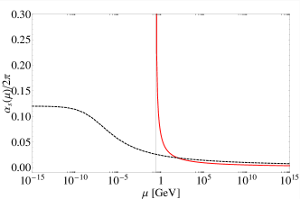
Figure 1: The strong running coupling $\alpha_{s}(\mu)$ for $N_{f}=12$ (Black Dashed) and for $N_{f}=5$ (Solid Red).

I.3 Thrust at NNLO

The thrust ($T$) variable is defined as

$$T=\frac{\max\limits_{\vec{n}}\sum\limits_{i}|\vec{p}_{i}\cdot\vec{n}|}{\sum\limits_{i}|\vec{p}_{i}|},$$ (9)

where the sum runs over all particles in the hadronic final state, and the $\vec{p}_{i}$ denotes the three-momentum of particle $i$. The unit vector $\vec{n}$ is varied to maximize thrust $T$, and the corresponding $\vec{n}$ is called the thrust axis and denoted by $\vec{n}_{T}$. It is often used the variable $(1-T)$, which for the LO of the 3 jet production is restricted to the range $(0<1-T<1/3)$. We have a back-to-back or a spherically symmetric event respectively at $T=1$ and at $T=2/3$ respectively.
In general a normalized IR safe single variable observable, such as the thrust distribution for the $e^{+}e^{-}\rightarrow 3jets$ DelDuca:2016ily ; DelDuca:2016csb , is the sum of pQCD contributions calculated up to NNLO at the initial renormalization scale $\mu_{0}=\sqrt{s}=M_{Z_{0}}$:

$$\frac{1}{\sigma_{tot}}\!\frac{Od\sigma(\mu_{0})}{dO}\! = \left\{x_{0}\cdot\frac{Od\bar{A}_{\mathit{O}}(\mu_{0})}{dO}+x_{0}^{2}\cdot\frac{Od\bar{B}_{\mathit{O}}(\mu_{0})}{dO}\right.$$ (10)

$$+\left.x_{0}^{3}\cdot\frac{Od\bar{C}_{\mathit{O}}(\mu_{0})}{dO}+{\cal O}(\alpha_{s}^{4})\right\},$$

where $O$ is the selected Event Shape variable, $\sigma$ the cross section of the process,

$$\sigma_{tot}=\sigma_{0}\left(1+x_{0}A_{tot}+x_{0}^{2}B_{tot}+{\cal O}\left(\alpha_{s}^{3}\right)\right)$$

is the total hadronic cross section and $\bar{A}_{O},\bar{B}_{O},\bar{C}_{O}$ are respectively the normalized LO, NLO and NNLO coefficients:

$$\bar{A}_{O} = A_{O}$$

$$\bar{B}_{O} = B_{O}-A_{tot}A_{O}$$ (11)

$$\bar{C}_{O} = C_{O}-A_{tot}B_{O}-\left(B_{tot}-A_{tot}^{2}\right)A_{O}.$$

where $A_{O},B_{O},C_{O}$ are the coefficients normalized to the tree level cross section $\sigma_{0}$ calculated by MonteCarlo (see e.g. EERAD and Event2 codes Gehrmann-DeRidder:2007nzq ; GehrmannDeRidder:2007hr ; Ridder:2014wza ; Weinzierl:2008iv ; Weinzierl:2009ms ) and $A_{\mathit{tot}},B_{\mathit{tot}}$ are:

$$A_{\mathit{tot}} = \frac{3}{2}C_{F};$$

$$B_{\mathit{tot}} = \frac{C_{F}}{4}N_{c}+\frac{3}{4}C_{F}\frac{\beta_{0}}{2}(11-8\zeta(3))-\frac{3}{8}C_{F}^{2}.$$ (12)

where $\zeta$ is the Riemann zeta function.

According to the PMC_∞ (for an introduction on the PMC_∞ see Ref. DiGiustino:2020fbk ) Eq.10 becomes:

$$\frac{1}{\sigma_{tot}}\!\frac{Od\sigma(\mu_{I},\tilde{\mu}_{II},\mu_{0})}{dO}=\left\{\overline{\sigma}_{I}+\overline{\sigma}_{II}+\overline{\sigma}_{III}+{\cal O}(\alpha_{s}^{4})\right\},$$ (13)

where the $\overline{\sigma}_{N}$ are normalized subsets that are given by:

$$\overline{\sigma}_{I} = A_{\mathit{Conf}}\cdot x_{I}$$

$$\overline{\sigma}_{II} = \left(B_{\mathit{Conf}}+\eta A_{\mathit{tot}}A_{\mathit{Conf}}\right)\cdot x_{II}^{2}-\eta A_{\text{tot}}A_{\mathit{Conf}}\cdot x_{0}^{2}$$

$$-A_{\text{tot}}A_{\mathit{Conf}}\cdot x_{0}x_{I}$$

$$\overline{\sigma}_{III} = \!\!\left(C_{\mathit{Conf}}\!-\!A_{\text{tot}}\!B_{\mathit{Conf}}\!-\!(B_{\text{tot}}-A_{\text{tot}}^{2})A_{\mathit{Conf}}\right)\cdot x_{0}^{3},$$

$A_{\mathit{Conf}},B_{\mathit{Conf}},C_{\mathit{Conf}}$ are the scale invariant conformal coefficients (i.e. the coefficients of each perturbative order not depending on the scale $\mu_{R}$) while $x_{I},x_{II},x_{0}$ are the couplings determined at the $\mu_{I},\tilde{\mu}_{II},\mu_{0}$ scales respectively. The PMC_∞ scales, $\mu_{N}$ , are given by:

$$\large{\mu}_{\mathit{I}} = \sqrt{s}\cdot e^{f_{sc}-\frac{1}{2}B_{\beta_{0}}},\hskip 54.06006pt{\scriptstyle(1-T)<0.33}$$

$$\large{\tilde{\mu}}_{\mathit{II}} = \left\{\begin{array}[]{lr}\sqrt{s}\cdot e^{f_{sc}-\frac{1}{2}C_{\beta_{0}}\cdot\frac{B_{\mathit{Conf}}}{B_{\mathit{Conf}}+\eta\cdot A_{\mathit{tot}}A_{\mathit{Conf}}}},\\ \hskip 110.96556pt{\scriptstyle(1-T)<0.33}\\ \sqrt{s}\cdot e^{f_{sc}-\frac{1}{2}C_{\beta_{0}}},\\ \hskip 110.96556pt{\scriptstyle(1-T)>0.33}\\ \end{array}\right.$$ (19)

and $\mu_{0}=M_{Z_{0}}$. The renormalization scheme factor for the QCD results is set to $f_{sc}\equiv 0$. The coefficients $B_{\beta_{0}},C_{\beta_{0}}$ are the coefficients related to the $\beta_{0}$-terms of the NLO and NNLO perturbative order of the thrust distribution respectively. They are determined from the calculated $A_{O},B_{O},C_{O}$ coefficients by using the iCF (the intrinsic conformality DiGiustino:2020fbk ).

The $\eta$ parameter is a regularization term in order to cancel the singularities of the NLO scale, $\mu_{II}$, in the range $(1-T)<0.33$, depending on non-matching zeroes between numerator and denominator in the $C_{\beta_{0}}$. In general this term is not mandatory for applying the PMC_∞, it is necessary only in case one is interested to apply the method all over the entire range covered by the thrust, or any other observable. Its value has been determined to $\eta=3.51$ for the thrust distribution and it introduces no bias effects up to the accuracy of the calculations and the related errors are totally negligible up to this stage.

II The thrust distribution according to $N_{f}$

Results for the thrust distribution calculated using the NNLO solution for the coupling $\alpha_{s}(\mu)$, at different values of the number of flavors, $N_{f}$, is shown in Fig. 2.

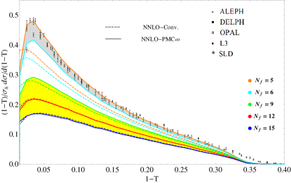
Figure 2: Thrust distributions for different values of $N_{f}$, using the PMC_∞ (Solid line) and the CSS (Dashed line). The Yellow shaded area is the results for the values of $N_{f}$ taken in the conformal window. The experimental data points are taken from the ALEPH, DELPHI,OPAL, L3, SLD experiments aleph ; delphi ; opal ; l3 ; sld .

A direct comparison between PMC_∞ (Solid line) and CSS (Dashed line) is shown at different values of the number of flavors. We notice that, despite the phase transition (i.e. the transition from an infrared finite coupling to an infrared diverging coupling), the curves given by the PMC_∞ at different $N_{f}$, preserve with continuity the same characteristics of the conformal distribution setting $N_{f}$ out of the conformal window of pQCD. In fact, the position of the peak of the thrust distribution is well preserved varying the $N_{f}$ in and out of the conformal window using the PMC_∞, while there is constant shift towards lower values using the CSS. These trends are shown in Fig. 3. We notice that in the central range, $2<N_{f}<15$, the position of the peak is exactly preserved using the PMC_∞ and overlaps with the position of the peak shown by the experimental data. According to our analysis for the case PMC_∞, in the range, $N_{f}<2$ the number of bins is not enough to resolve the peak, though the behavior of the curve is consistent with the presence of a peak in the same position, while for $N_{f}\rightarrow 0$ the peak is no longer visible. Theoretical uncertainties on the position of the peak have been calculated using standard criteria, i.e. varying the remaining initial scale value in the range $M_{Z_{0}}/2\leq\mu_{0}\leq 2M_{Z_{0}}$, and considering the lowest uncertainty given by the half of the spacing between two adjacent bins.

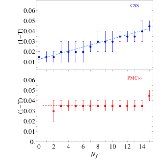
Figure 3: Comparison of the position of the peak for the thrust distribution using the CSS and the PMC_∞ vs the number of flavors, $N_{f}$. Dashed Lines indicate the particular trend in each graph.

Using the definition given in Ref. Gehrmann-DeRidder:2007nzq of the parameter

$$\delta=\frac{\text{max}_{\mu}(\sigma(\mu))-\text{min}_{\mu}(\sigma(\mu))}{2\sigma(\mu=M_{Z_{0}})},$$ (20)

with the renormalization scale varying $\mu\in[M_{Z_{0}}/2;2M_{Z_{0}}]$, we have determined the average error, $\bar{\delta}$, calculated in the interval $0.005<(1-T)<0.4$ of the thrust and results for CSS and PMC_∞ are shown in Fig. 4. We notice that the PMC_∞ in the perturbative and IR conformal window, i.e. $12<N_{f}<\bar{N}_{f}$, which is the region where $\alpha_{s}(\mu)<1$ in the whole range of the renormalization scale values, from $0$ up to $\infty$, the average error given by PMC_∞ tends to zero ($\sim 0.23-0.26\%$) while the error given by the CSS tends to remain constant ($0.85-0.89\%$). The comparison of the two methods shows that, out of the conformal window, $N_{f}<\frac{34N_{c}^{3}}{13N_{c}^{2}-3}$, the PMC_∞ leads to a higher precision.

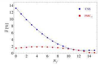
Figure 4: Comparison of the average theoretical error, $\bar{\delta}$, calculated using standard criteria in the range: $0.005<(1-T)<0.4$, using the CSS and the PMC_∞ for the thrust distribution vs the number of flavors, $N_{f}$.

III The thrust distribution in the Abelian limit $N_{c}\rightarrow 0$

We obtain the QED thrust distribution performing the $N_{c}\rightarrow 0$ limit of the QCD thrust at NNLO according to Brodsky:1997jk ; Kataev:2015yha . In the zero number of colors limit the gauge group color factors are fixed by $N_{A}=1,C_{F}=1,T_{R}=1,C_{A}=0,N_{c}=0,N_{f}=N_{l}$, where $N_{l}$ is the number of active leptons, while the $\beta$-terms and the coupling rescale as $\beta_{n}/C_{F}^{n+1}$ and $\alpha_{s}\cdot C_{F}$ respectively. In particular $\beta_{0}=-\frac{4}{3}N_{l}$ and $\beta_{1}=-4N_{l}$ using the normalization of Eq. 1. According to these rescaling of the color factors we have determined the QED thrust and the QED PMC_∞ scales. For the QED coupling , we have used the analytic formula for the effective fine structure constant in the $\overline{\text{MS}}$-scheme:

$${\alpha(Q^{2})}={\alpha\over{\left(1-\Re e\Pi^{\overline{\text{MS}}}(Q^{2})\right)}},$$ (21)

with $\alpha^{-1}\equiv\alpha(0)^{-1}=137.036$ and the vacuum polarization function ($\Pi$) calculated perturbatively at two loops including contributions from leptons, quarks and $W$ boson. The QED PMC_∞ scales have the same form of Eq. 19 with the factor for the $\overline{\text{MS}}$-scheme set to $f_{sc}\equiv 5/6$ and the $\eta$ regularization parameter introduced to cancel singularities in the NLO PMC_∞ scale $\mu_{II}$ in the $N_{c}\rightarrow 0$ limit tends to the same QCD value, $\eta=3.51$. A direct comparison between QED and QCD PMC_∞ scales is shown in Fig. 5.

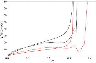
Figure 5: PMC_∞ scales for the thrust distribution: LO-QCD scale (Solid Red); LO-QED scale (Solid Black);NLO-QCD scale (Dashed Red); NLO-QED scale (Dashed Black).

We notice that in the QED limit the PMC_∞ scales have analogous dynamical behavior as those calculated in QCD, differences arise mainly by the $\overline{\text{MS}}$ scheme factor reabsorption, the effects of the $N_{c}$ number of colors at NLO are very small. Thus we notice that perfect consistency is shown from QCD to QED using the PMC_∞ method. The normalized QED thrust distribution is shown in Fig. 6. We notice that the curve is peaked at the origin, $T=1$, which suggests that the three jet event in QED occurs with a rather back-to-back symmetry. Results for the CSS and the PMC_∞ methods in QED are of the order of $O(\alpha)$ and given the good convergence of the theory the results for the two methods show very small differences.

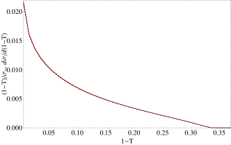
Figure 6: Thrust distributions in the QED limit at NNLO using the PMC_∞ (Solid Red) and the CSS (Dashed Black).

IV Conclusions

We have investigated, for the first time, the thrust distribution in the conformal window of pQCD. Assuming, for phenomenological reasons, the physical value of the strong coupling to be the one at the $Z_{0}$ mass scale it restricts the conformal window range, at two loops, to be within $\frac{34N_{c}^{3}}{13N_{c}^{2}-3}<N_{f}<\bar{N}_{f}$ with $\bar{N}_{f}\simeq 15.22$. The closer $N_{f}$ to the higher value the more perturbative and conformal the system is. In this region, we have shown that the PMC_∞ leads to a higher precision with a theoretical error which tends to zero. Besides results for the thrust distribution in the conformal window have similar shapes to those of the physical values of $N_{f}$ and the position of the peak is preserved when one applies the PMC_∞ method. Comparison with the experimental data indicates also that PMC_∞ agrees with the expected number of flavors. A good fit with experimental data is shown by the PMC_∞ results for the range $5<N_{f}<6$, which agrees with the active number of flavors of the Standard Model. Outside the pQCD conformal window the PMC_∞ leads to a higher precision with respect to the CSS. In addition, calculations for the QED thrust reveal a perfect consistency of the PMC_∞ with QED when taking the QED limit of QCD for both the PMC_∞ scale and for the regularization $\eta$ parameter which tends to the same QCD value.

Acknowledgements: We thank Stanley J. Brodsky for his valuable comments and for useful discussions. We thank Einan Gardi and Philip G. Ratcliffe for helpful discussions.

References

- (1) D. D. Dietrich and F. Sannino, Phys. Rev. D 75 (2007), 085018 doi:10.1103/PhysRevD.75.085018 [arXiv:hep-ph/0611341 [hep-ph]].
- (2) G. Cacciapaglia, C. Pica and F. Sannino, Phys. Rept. 877 (2020), 1-70 doi:10.1016/j.physrep.2020.07.002 [arXiv:2002.04914 [hep-ph]].
- (3) O. Antipin and F. Sannino, Phys. Rev. D 97 (2018) no.11, 116007 doi:10.1103/PhysRevD.97.116007 [arXiv:1709.02354 [hep-ph]].
- (4) T. Banks, A. Zaks, Nuclear Physics B. Elsevier BV. 196 (2): 189-204 (1982).
- (5) C. Pica and F. Sannino, Phys. Rev. D 83 (2011), 035013 doi:10.1103/PhysRevD.83.035013 [arXiv:1011.5917 [hep-ph]].
- (6) T. A. Ryttov and R. Shrock, Phys. Rev. D 83 (2011), 056011 doi:10.1103/PhysRevD.83.056011 [arXiv:1011.4542 [hep-ph]].
- (7) T. A. Ryttov and R. Shrock, Phys. Rev. D 94 (2016) no.10, 105015 doi:10.1103/PhysRevD.94.105015 [arXiv:1607.06866 [hep-th]].
- (8) S. Kluth, Rept. Prog. Phys. 69, 1771 (2006).
- (9) A. Heister et al. [ALEPH Collaboration], Eur. Phys. J. C 35, 457 (2004).
- (10) J. Abdallah et al. [DELPHI Collaboration], Eur. Phys. J. C 29, 285 (2003).
- (11) G. Abbiendi et al. [OPAL Collaboration], Eur. Phys. J. C 40, 287 (2005).
- (12) P. Achard et al. [L3 Collaboration], Phys. Rept. 399, 71 (2004).
- (13) K. Abe et al. [SLD Collaboration], Phys. Rev. D 51, 962 (1995).
- (14) R. K. Ellis, D. A. Ross and A. E. Terrano, Nucl. Phys. B 178, 421 (1981).
- (15) Z. Kunszt, Phys. Lett. 99B, 429 (1981).
- (16) J. A. M. Vermaseren, K. J. F. Gaemers and S. J. Oldham, Nucl. Phys. B 187, 301 (1981).
- (17) K. Fabricius, I. Schmitt, G. Kramer and G. Schierholz, Z. Phys. C 11, 315 (1981).
- (18) W. T. Giele and E. W. N. Glover, Phys. Rev. D 46, 1980 (1992).
- (19) S. Catani and M. H. Seymour, Phys. Lett. B 378, 287 (1996).
- (20) A. Gehrmann-De Ridder, T. Gehrmann, E. W. N. Glover and G. Heinrich, Phys. Rev. Lett. 99, 132002 (2007).
- (21) A. Gehrmann-De Ridder, T. Gehrmann, E. W. N. Glover and G. Heinrich, JHEP 0712, 094 (2007).
- (22) A. Gehrmann-De Ridder, T. Gehrmann, E. W. N. Glover and G. Heinrich, Comput. Phys. Commun. 185, 3331 (2014).
- (23) S. Weinzierl, Phys. Rev. Lett. 101, 162001 (2008).
- (24) S. Weinzierl, JHEP 0906, 041 (2009).
- (25) R. Abbate, M. Fickinger, A. H. Hoang, V. Mateu and I. W. Stewart, Phys. Rev. D 83, 074021 (2011).
- (26) A. Banfi, H. McAslan, P. F. Monni and G. Zanderighi, JHEP 1505, 102 (2015).
- (27) M. Tanabashi et al. [Particle Data Group], Phys. Rev. D 98, 030001 (2018).
- (28) M. Gell-Mann and F. E. Low, Phys. Rev. 95, 1300 (1954).
- (29) M. Beneke, Phys. Rept. 317, 1 (1999).
- (30) S. J. Brodsky, G. P. Lepage and P. B. Mackenzie, Phys. Rev. D 28, 228 (1983) doi:10.1103/PhysRevD.28.228
- (31) S. J. Brodsky and L. Di Giustino, Phys. Rev. D 86, 085026 (2012).
- (32) S. J. Brodsky and X. G. Wu, Phys. Rev. D 85, 034038 (2012).
- (33) S. J. Brodsky and X. G. Wu, Phys. Rev. Lett. 109, 042002 (2012).
- (34) M. Mojaza, S. J. Brodsky and X. G. Wu, Phys. Rev. Lett. 110, 192001 (2013).
- (35) S. J. Brodsky, M. Mojaza and X. G. Wu, Phys. Rev. D 89, 014027 (2014).
- (36) S. J. Brodsky and X. G. Wu, Phys. Rev. D 86, 054018 (2012).
- (37) X. G. Wu, Y. Ma, S. Q. Wang, H. B. Fu, H. H. Ma, S. J. Brodsky and M. Mojaza, Rept. Prog. Phys. 78, 126201 (2015).
- (38) S. J. Brodsky and P. Huet, Phys. Lett. B 417, 145 (1998).
- (39) L. Di Giustino, S. J. Brodsky, S. Q. Wang and X. G. Wu, Phys. Rev. D 102, no.1, 014015 (2020) doi:10.1103/PhysRevD.102.014015 [arXiv:2002.01789 [hep-ph]].
- (40) S. Q. Wang, S. J. Brodsky, X. G. Wu and L. Di Giustino, Phys. Rev. D 99, no.11, 114020 (2019) doi:10.1103/PhysRevD.99.114020 [arXiv:1902.01984 [hep-ph]].
- (41) S. Q. Wang, S. J. Brodsky, X. G. Wu, J. M. Shen and L. Di Giustino, Phys. Rev. D 100, no.9, 094010 (2019) doi:10.1103/PhysRevD.100.094010 [arXiv:1908.00060 [hep-ph]].
- (42) D. J. Gross and F. Wilczek, Phys. Rev. Lett. 30, 1343-1346 (1973) doi:10.1103/PhysRevLett.30.1343
- (43) H. D. Politzer, Phys. Rev. Lett. 30, 1346-1349 (1973) doi:10.1103/PhysRevLett.30.1346
- (44) W. E. Caswell, Phys. Rev. Lett. 33, 244 (1974) doi:10.1103/PhysRevLett.33.244
- (45) D. R. T. Jones, Nucl. Phys. B 75, 531 (1974) doi:10.1016/0550-3213(74)90093-5
- (46) E. Egorian and O. V. Tarasov, Teor. Mat. Fiz. 41, 26-32 (1979) JINR-E2-11757.
- (47) P. A. Zyla et al. [Particle Data Group], PTEP 2020, no.8, 083C01 (2020) doi:10.1093/ptep/ptaa104
- (48) E. Gardi, G. Grunberg and M. Karliner, JHEP 07, 007 (1998) doi:10.1088/1126-6708/1998/07/007 [arXiv:hep-ph/9806462 [hep-ph]].
- (49) A. Deur, S. J. Brodsky and G. F. de Teramond, Nucl. Phys. 90, 1 (2016) doi:10.1016/j.ppnp.2016.04.003 [arXiv:1604.08082 [hep-ph]].
- (50) T. A. Ryttov and R. Shrock, Phys. Rev. D 96, no.10, 105018 (2017) doi:10.1103/PhysRevD.96.105018 [arXiv:1706.06422 [hep-th]].
- (51) V. Del Duca, C. Duhr, A. Kardos, G. Somogyi and Z. Trocsanyi, Phys. Rev. Lett. 117, 152004 (2016).
- (52) V. Del Duca, C. Duhr, A. Kardos, G. Somogyi, Z. Szor, Z. Trocsanyi and Z. Tulipant, Phys. Rev. D 94, 074019 (2016).
- (53) A. L. Kataev and V. S. Molokoedov, Phys. Rev. D 92, no.5, 054008 (2015) doi:10.1103/PhysRevD.92.054008 [arXiv:1507.03547 [hep-ph]].