System identification using Bayesian neural networks with nonparametric noise models

\@ADDCLASS{ltx_runin}0. Abstract

System identification is of special interest in science and engineering. This article is concerned with a system identification problem arising in stochastic dynamic systems, where the aim is to estimate the parameters of a system along with its unknown noise processes. In particular, we propose a Bayesian nonparametric approach for system identification in discrete time nonlinear random dynamical systems assuming only the order of the Markov process is known. The proposed method replaces the assumption of Gaussian distributed error components with a highly flexible family of probability density functions based on Bayesian nonparametric priors. Additionally, the functional form of the system is estimated by leveraging Bayesian neural networks which also leads to flexible uncertainty quantification. Asymptotically on the number of hidden neurons, the proposed model converges to full nonparametric Bayesian regression model. A Gibbs sampler for posterior inference is proposed and its effectiveness is illustrated on simulated and real time series.

Keywords: Bayesian nonparametrics; System identification; Infinite mixture models; Nonlinear time series; Geometric stick breaking

1. Introduction

Random dynamical systems, that is, dynamical systems that evolve through the presence of noise, play an important role in science and engineering as they can be used to model and explain dependencies in physical phenomena changing in time. This noise may be observational, attributed to measurement errors from the measuring device, or dynamical which compensates for modeling error or both. Common areas of application include but are not limited to neuroscience, finance (Franses et al., 2000; Small, 2005; Ozaki, 2012), and signal processing (Lau and Tse, 2003).

In this article, we consider dynamical systems that are observed in the form of a time series and the mathematical model describing the process is given by

$$y_{t}=g(y_{t}^{\rho};\theta)+z_{t},\quad t=1,2,\ldots$$ (1)

where $y_{t}$ is the observed process and the vector $y_{t}^{\rho}:=(y_{t-1},\ldots,y_{t-\rho})$ consists of a set of lagged versions of the process $y_{t}$ which allows the system to be written in the form of a regression model. Additionally, $\theta$ is a vector of parameters $\theta:=(\theta_{1},\ldots,\theta_{m})$ and $\{z_{t}\}_{t\geq 1}$ is a collection of i.i.d. zero-mean noise components with finite variance. For simplicity, we assume that we have at our disposal a time series of length $n$ generated from (1) and that the vector of $\rho$ initial states is known.

System identification refers to the problem of accurate estimation of $\hat{g}$ or, equivalently, $\hat{\theta}$ that describes the observed process well enough in order to understand the dynamics and use it for control and/or prediction of future unobserved values of the system (Sjöberg et al., 1995; Ljung, 1999; Nelles, 2001; Keesman, 2011). System identification is typically done with some statistical method for estimating the parameters based on the available data.

For a discrete-time scalar time series $\{y_{t}\}_{t\geq 1},$ the Box–Jenkins (Box et al., 2015) modeling approach is to assume an autoregressive integrated moving average $\mathrm{ARIMA}(p,d,q)$ model for $\{y_{t}\}.$ In this framework, a non-stationary time series is differentiated $d$ times to become stationary and then a suitable model for representing the process $y_{t}$ is $\mathrm{\Omega}_{p}(B)y_{t}=\mathrm{\Psi}_{q}(B)z_{t},$ where

$$\mathrm{\Omega}_{p}(B) =1-\omega_{1}B-\cdots-\omega_{p}B^{p},$$

$$\mathrm{\Psi}_{q}(B) =1-\psi_{1}B-\cdots-\psi_{q}B^{q}$$ (2)

are polynomials of degree $p,q$ respectively of the backshift operator $B,$ with $B^{\rho}y_{t}=y_{t-\rho}.$ The polynomial degrees, and the coefficients $\theta=(\omega_{1},\ldots,\omega_{p},\psi_{1},\ldots,\psi_{q})$ of the polynomials are estimated from the observed data. These models work extremely well for linear Gaussian time series, however, they are not sufficient for nonlinear or chaotic time series modeling. To this end, more sophisticated, nonlinear models for the function $g$ have been developed. Some of the popular choices include, among others, the bilinear model, the threshold autoregressive model along with the extension to self-exciting threshold autoregressive model (Tong and Lim, 1980) and the autoregressive conditional heteroscedasticity (ARCH) model (Engle, 1982). Moreover, black-box nonlinear models using artificial neural networks have been successfully used for nonlinear time series estimation and prediction (Chen and Billings, 1992; Sjöberg et al., 1994, 1995; Zhang, 2003; Aladag et al., 2009).

The so-called Bayesian approaches (Gelman et al., 2013) incorporate prior information in terms of probability distributions to the estimation process. Bayesian methods have been used to estimate the parameters of maps responsible for the generation of chaotic signals contaminated with Gaussian noise (Luengo et al., 2002; Meyer and Christensen, 2000; Pantaleón et al., 2000, 2003). In all cases above, the general functional form of the system in question is known and the aim is to estimate the control parameters. Bayesian methods have also been used (Pantaleón et al., 2003) to estimate piecewise Markov systems. Slightly similarly, in the context of Bayesian estimation but, regarding dynamically noise-corrupted signals and taking a black-box approach, (Matsumoto et al., 2001; Nakada et al., 2005) developed hierarchical Bayesian methods for the reconstruction and prediction of random dynamical systems. More recently, there has been increasing research interest in the development of Gaussian process (Rasmussen and Williams, 2006) models for black-box time series modeling (Kocijan et al., 2005; Turner et al., 2009; Bijl et al., 2017; Särkkä et al., 2018).

A common feature of most of the aforementioned methods is that they are based on the rather strong assumption of Gaussian noise which is rarely true in real world applications and is typically chosen for computational convenience. Other choices, based on scaled mixtures of Gaussians have also been proposed (Ishwaran and Rao, 2005; Polson and Scott, 2010; Carvalho et al., 2010) however, these choices are still parametric capturing only a bounded amount of information in the data. On the other hand, restricting $g$ to belong to a particular class of functions might be difficult when there is not enough information for the problem at hand, leading to models with poor generalization capabilities.

In this paper, we aim to develop hierarchical Bayesian models for the estimation and prediction of random dynamical systems from observed time series data. In particular, we use a nonparametric Bayesian prior namely, the geometric stick breaking process (GSB) prior introduced by Fuentes-Garcia et al. (2010) which allows for flexible modeling of unknown distributions in order to drop the common assumption of Gaussian distributed noise components. Bayesian nonparametric modeling of the noise process has been successfully attempted before (Hatjispyros et al., 2009; Merkatas et al., 2017; Hatjispyros and Merkatas, 2019) in the context of dynamical reconstruction from observed time series data. Our model is an extension of the model proposed at Merkatas et al. (2017) where we additionally aim to adopt a black-box modeling approach that does minimal assumptions for the data at hand. In particular, we drop the assumption of a known functional form of the deterministic part of the system by leveraging Bayesian neural networks (Neal, 1996). We parametrize the data generating mechanism with a feed-forward neural network whose weights and biases are assigned a prior distribution. In the limit of infinite hidden neurons a priori, this neural network converges to a Gaussian process prior (cf. Neal, 1996) making the approach completely nonparametric. This makes our model flexible and suitable for modeling real time series data, requiring only the order of the underlying Markov process to be known. Recent advances in embedding dimensions and signature learning (Fermanian, 2021) may provide additional information on how to select the lag in the inferential process but this is beyond the scope of this paper.

It should be stressed that a purely Bayesian nonparametric approach to the problem described here would be a density regression approach. In density regression, the functional form of the system and the noise process are assumed unknown and the use of the so called dependent nonparametric priors is required (Fuentes-García et al., 2009; Hatjispyros et al., 2018; Lijoi et al., 2014; Mena et al., 2011). However, the construction of such priors can be hard especially for continuous time series modeling because dependencies among the random probability measures changing in time would require analytical solutions to stochastic differential equations or, at least, efficient computational methods. Our framework can be extended to continuous time modeling using more sophisticated neural network architectures, for example, neural ordinary differential equations (Chen et al., 2018).

The paper is organized as follows. Section 2 introduces the necessary background on Bayesian nonparametric models and Bayesian neural networks. The proposed model for estimation and prediction of random dynamical systems is derived in Section 3. Next, in Section 4 we introduce a fast MCMC sampling algorithm for posterior inference based on a Gibbs kernel and we show how the samples taken from the posterior can be used for prediction of future values. Experimental evaluation in simulated and real data is given in Section 5. Finally, we conclude and discuss the results in Section 6.

2. Background

In this section we provide the necessary background for the building blocks of the proposed model. We start with the review of Bayesian neural networks (Neal, 1996) and the Hamiltonian Monte Carlo (HMC) method for posterior inference (Kennedy, 1988) which is crucial for the update of the neural network weights within our Gibbs sampler. For completeness, an introduction to nonparametric priors (Hjort et al., 2010) and their application in mixture modeling is given in Section 2.2.

2.1. Bayesian neural networks

Feed-forward neural networks are popular models for estimating functions from data due to their universal approximation property (Cybenko, 1989). For our purposes we focus on a feed-forward neural network with $L$ layers where each layer consists of $N_{l},\,0\leq l\leq L$ neurons. The parameters of the neural network are given by a set of weight matrices $W^{(l)}:=(W^{(l)}_{ij})^{i=1:N_{l}}_{j=1:N_{l}-1}$ and bias vectors $b^{(l)}:=(b^{(l)}_{i})_{i=1:N_{l}}$ collectively denoted by $\theta,$ that is, $\theta=\{W^{(l)},b^{(l)}\}_{l=1}^{L}.$ The network computes functions $y=g(x;\theta)$ by forward-propagating the inputs as follows. In each layer $l=1,\ldots,L$ the network computes the affine transformation $a^{(l)}:=W^{(l)}x^{(l-1)}+b^{(l)}$ to its input and applies an elementwise nonlinearity as $x^{(l)}:=h^{(l)}(a^{(l)})$ where, $x:=x^{(0)}$ and $y:=x^{(L)}.$ Typical choices for the nonlinear function $h$ include the hyperbolic tangent, the logistic function, and more recently, the rectified linear unit function (Goodfellow et al., 2016). Since we are going to use the network for regression tasks, the function at the output layer $h^{(L)}$ is chosen to be the linear function while for $l<L$ we choose the $\tanh$ activation function.

The neural network becomes Bayesian (MacKay, 1992; Nowlan and Hinton, 1992; Neal, 1996) when a prior distribution is assigned on the parameters $\theta$ and predictions are made using the posterior predictive distribution of the model. The Bayesian neural network can be written in hierarchical fashion as

$$y_{t}\mid x_{t},\theta,\lambda\sim\mathrm{N}(y_{t}\mid g(x_{t};\theta),\Lambda^{-1}),\quad 1\leq t\leq n,$$ (3)

$$\theta\sim p(\theta\mid\tau),\,\tau\sim p(\tau),\,\Lambda\sim p(\Lambda),$$ (4)

where $(x_{t},y_{t}),\,1\leq t\leq n$ are the training data, $\Lambda$ is the precision matrix, and $\tau$ is a hyperparameter for the weights. Bayesian inference proceeds by sampling from the full posterior distribution given by

$$p(\theta,\Lambda,\tau\mid\{(x_{t},y_{t})\}_{t=1}^{n})\propto p(\Lambda)p(\tau)p(\theta\mid\tau)\prod_{t=1}^{n}\mathrm{N}(y_{t}\mid g(x_{t};\theta),\Lambda^{-1}).$$ (5)

It is possible to sample the parameters of a Bayesian model via MCMC. As we will see later, in Sect. 4.1, we can sample the parameters of our model by using a combination of MCMC methods namely, Gibbs (Geman and Geman, 1984) and Hamiltonian Monte Carlo (HMC) (Kennedy, 1988). In particular, HMC will be used to sample from the full conditional distribution of the neural network parameters $p(\theta\mid\cdots)$ which for now we denote by $p^{|{\cal D}}(\theta).$ After Neal’s seminal work (Neal, 1996), a sample for the weights is typically obtained from $p^{|{\cal D}}(\theta)$ via HMC (Neal et al., 2011) due to its complex geometry.

In HMC, a new sample is proposed in the parameter space using gradient information instead of simple random walk proposals. Introducing auxiliary variables $\eta$, where $\dim{\eta}=\dim{\theta},$ an ergodic Markov chain with stationary distribution the desired posterior distribution $p(\theta,\eta)=p^{|{\cal D}}(\theta)p(\eta)$ is constructed. This posterior can be seen as the canonical distribution of the joint state $(\theta,\eta)$ corresponding to the Hamiltonian energy function $H(\theta,\eta)=U(\theta)+T(\eta)=-\log p^{|{\cal D}}(\theta)+\frac{1}{2}\eta^{\top}M^{-1}\,\eta,$ where $M$ is a positive definite mass matrix.

Given the current state $(\theta,\eta)$ of the sampler, an HMC transition is given by first simulating new variables $\eta^{\prime}\sim p(\eta)$. Then, the new $\theta^{\prime}$ is proposed simulating a trajectory according to Hamilton’s equation of motion $(\dot{\theta},\dot{\eta})=(\partial_{\eta}H,-\partial_{\theta}H)$ using leapfrog integrator, a symplectic integrator which alternates between the following updates

$$\eta(\kappa+\epsilon/2) =\eta(\kappa)-\frac{\epsilon}{2}\partial_{\theta}H(\theta(\kappa),\eta(\kappa))$$

$$\theta(\kappa+\epsilon) =\theta(\kappa)+\epsilon\partial_{\eta}H(\theta(\kappa),\eta(\kappa+\epsilon/2))$$

$$\eta(\kappa+\epsilon) =\eta(\kappa+\epsilon/2)-\frac{\epsilon}{2}\partial_{\theta}H(\theta(\kappa+\epsilon),\eta(\kappa+\epsilon/2)),$$

where $\epsilon$ is the discretization step length, $S$ is the number of steps giving a trajectory of length $\epsilon S$, and $\kappa$ is the time variable.

To account for trajectory simulation errors, a Metropolis acceptance step is included and the proposed state is accepted with probability

$$\mathrm{acc}(\theta^{\prime},\theta)=\min\{1,p(\theta^{\prime},\eta^{\prime})/p(\theta,\eta)\}.$$ (6)

2.2. Bayesian nonparametrics

Bayesian nonparametrics dates back to introduction of Dirichlet processes (DPs) (Ferguson, 1973) but has been widely used only after the development of Markov chain Monte Carlo (MCMC) (Brooks et al., 2011) methods. Their main advantage in statistical and machine learning applications is their ability to adapt their complexity according to the available data, using a potentially infinite number of parameters. In this section we provide some background material on Bayesian nonparametric priors and their application on mixture modeling.

A general random discrete distribution on the space $(\Xi,\sigma(\Xi))$ where $\sigma(\Xi)$ is the Borel $\sigma$-algebra of subsets of $\Xi$ can be represented as

$$\mathbb{P}=\sum_{k=1}^{K}\pi_{k}\delta_{\xi_{k}},$$ (7)

such that $\sum_{k=1}^{K}\pi_{k}=1\textrm{ a.s.}$ and $(\xi_{k})\stackrel{{\scriptstyle\mathrm{i.i.d}}}{{\sim}}P_{0},$ where $P_{0}$ is a non-atomic $\Xi-$valued measure. Allowing $K=\infty,$ standard results (Ongaro and Cattaneo, 2004) can be used to show that random probability measures of the form given in (7) have full support on the space $\mathcal{P}_{\Xi}$, the space of all probability measures defined on $\Xi.$ These random distributions can be used in the context of mixture models to define nonparametric mixtures. Convoluting the kernel of a parametric family with a random discrete distribution we can define mixture densities as

$$f(x\mid\mathbb{P})=\int_{\Xi}K(x\mid\xi)\mathbb{P}(\mathrm{d}\xi),\quad\mathbb{P}(\mathrm{d}\xi)=\sum_{k=1}^{K}\pi_{k}\delta_{\xi_{k}}(\mathrm{d}\xi).$$

Depending on the mechanism that the weights $\pi_{k}$ are constructed and if $K=\infty$ or not, different nonparametric mixture models can be recovered. Specifically, choosing $\mathbb{P}\sim\mathrm{DP}(c,P_{0})$ to be the Dirichlet process with mass $c>0$ and base measure $P_{0}$ (Sethuraman, 1994), that is,

$$\mathbb{P}=\sum_{k=1}^{\infty}\pi_{k}\delta_{\xi_{k}},\quad\xi_{k}\stackrel{{\scriptstyle\mathrm{i.i.d}}}{{\sim}}P_{0},$$ (8)

$$\pi_{k}=\phi_{j}\prod_{j<k}(1-\phi_{j}),\quad\phi_{1},\phi_{2}\ldots\stackrel{{\scriptstyle\mathrm{i.i.d}}}{{\sim}}\mathrm{Be}(1,c),$$ (9)

we recover the Dirichlet process mixture (DPM) model (Antoniak, 1974; Escobar and West, 1995) which is commonly used for density estimation problems.

Random probability measures, with less exotic weights can be obtained if we consider general random discrete distributions. In particular, Ishwaran and James (2001), introduced a general class of stick breaking distributions defined for $\phi_{k}\sim\mathrm{Be}(a_{k},b_{k})$ as in Equation (9), for $a_{k},b_{k}$ such that $\sum_{k=1}^{\infty}\log\mathbb{E}\left(1-\phi_{k}\right)=-\infty$ (Ghosal and Van der Vaart, 2017).

A rather interesting random discrete distribution is the geometric stick breaking process (GSB) (Fuentes-Garcia et al., 2010) which corresponds to a single beta random variable $\phi\sim\mathrm{Be}(a,b).$

$$\mathbb{P}=\sum_{k=1}^{\infty}\pi_{k}\delta_{\xi_{k}},\quad\xi_{k}\stackrel{{\scriptstyle\mathrm{i.i.d}}}{{\sim}}P_{0},$$ (10)

$$\pi_{k}=\phi(1-\phi)^{k-1},\quad\phi\sim\mathrm{Be}(a,b).$$ (11)

This random probability measure has full support on the space $\mathcal{P}_{\Xi},$ and in contrast to the Dirichlet process, its weights are almost surely decreasing. Later on, we will model the density of the noise components as a GSB mixture density.

Inference in mixture models proceeds with the introduction of a clustering variable for each observation that indicates the component of the mixture that the specific observation belongs to. However, the state space of the clustering variables is now countably infinite and additional auxiliary variables that make the sum finite have to be introduced (see for example, Walker (2007); Kalli et al. (2011) for the DPM model and beyond). We will provide details on this when we will construct the transition density for the observations of our model which we now introduce in Section 3. Nevertheless, the decreasing nature of the weights allows for faster sampling of the clustering variables leading to faster and less complicated sampling algorithms in contrast to the Dirichlet process counterpart.

3. Autoregressive Bayesian neural networks for time series modeling

In this section we present the Bayesian neural network model with a nonparametric noise component. We start with the development of a nonlinear autoregressive model in Section 3.1 and gradually extend it into a fully nonparametric method by introducing Bayesian neural networks as function approximators for the deterministic part and nonparametric noise components based on GSB mixtures.

3.1. Nonlinear autoregressive Bayesian neural network model

In this work we consider a discrete time dynamical system

$$y_{t}=g(y_{t}^{\rho},\theta)+z_{t},\quad 1\leq t\leq n,$$ (12)

where $g:\mathbb{R}^{D\times\rho}\times\Theta\to\mathbb{R}^{D}$ is a nonlinear function of $y_{t}^{\rho}:=(y_{t-1},\ldots,y_{t-\rho})$ parametrized by a vector of control parameters $\theta\in\Theta\subset\mathbb{R}^{m}.$ The random variables $z_{t}$ represent additive dynamical noise which for now we assume are i.i.d. samples from an unknown density $f(\cdot)$ taking values in $\mathbb{R}^{D}.$

In order to be able to capture nonlinearities in the time series with our model, a sufficiently expressive function should be chosen for $g(\cdot,\theta).$ To this end, we model the function responsible for the generation of the time series $g(\cdot,\theta)$ where $\theta=\{W^{(l)},b^{(l)}\}_{l=1}^{L},$ with a Bayesian neural network of $L$ layers as described in Section 2.1. The prior over the parameters in $\theta$ is taken to be Gaussian parametrized by precision $\bm{\tau}.$ In particular, we tie each group of weights and biases in a specific layer to their own precision $\tau_{W}^{(l)},\tau_{b}^{(l)}$ so that for $1\leq l\leq L:$

$$W^{(l)}\stackrel{{\scriptstyle\mathrm{ind}}}{{{.}\sim}}\mathrm{N}(0,[\tau_{W}^{(l)}]^{-1}),\quad b^{(l)}\stackrel{{\scriptstyle\mathrm{ind}}}{{{.}\sim}}\mathrm{N}(0,[\tau_{b}^{(l)}]^{-1}),$$ (13)

where $v\stackrel{{\scriptstyle\mathrm{ind}}}{{{.}\sim}}\nu$ denotes independently $\nu-$distributed elements $v_{i}$ of the vector/matrix $v.$ The precision parameters $\tau_{\bullet}^{(l)}$ control how much the weights/biases can vary in group $l$ and are further assigned Gamma hyperprior distributions $\mathrm{Ga}(\tau_{\bullet}^{(l)}\mid\alpha_{\tau_{\bullet}^{(l)}},\beta_{\tau_{\bullet}^{(l)}})$ with mean $\alpha_{\tau_{\bullet}^{(l)}}/\beta_{\tau_{\bullet}^{(l)}}.$ This way a hierarchical model for the weights and biases between layers is defined and information can be shared among different layers, a concept known as “borrowing of strength” (Gelman et al., 2013; Neal, 1996).

In the next section we adopt a Bayesian nonparametric mixture modeling approach for the density of the noise components. In particular, we aim to model the density of the noise components as an infinite mixture of Gaussian kernels based on the GSB process. This approach is nonparametric and is equivalent with placing a prior over the space of densities. Under the proposed setting, the model presented in Merkatas et al. (2017) is extended to a full nonparametric Bayesian model for system identification. Thus, the only necessary information is the order of the Markov process given in Equation (12) which allows us to form the regressors $y^{\rho}_{t}.$

3.2. Nonparametric noise process

Consider a general discrete random probability measure $\mathbb{P}=\sum_{k=1}^{\infty}\pi_{k}\delta_{\Lambda_{k}}$ defined as in Equation (7). The density of each component $z_{t}$ of the noise process can be modeled as an infinite mixture of (multivariate) Gaussian kernels

$$f(z_{t}\mid\mathbb{P})=\int_{\mathcal{M}^{+}}\mathrm{N}(z_{t}\mid\bm{0},\Lambda^{-1})\,\mathbb{P}(\mathrm{d}\Lambda)=\sum_{k=1}^{\infty}\pi_{k}\,\mathrm{N}(z_{t}\mid\bm{0},\Lambda_{k}^{-1}).$$ (14)

In the equation above, $\mathcal{M}^{+}$ denotes the set of positive semi-definite $D\times D$ precision matrices defined on $\mathbb{R},$ and $\bm{0}$ is the $D$-dimensional zero vector. From the additivity of the errors, the transition density for the observations reads

$$f(y_{t}\mid y^{\rho}_{t},\theta,(\pi_{k})_{k\geq 1},(\Lambda_{k})_{k\geq 1})=\sum_{k=1}^{\infty}\pi_{k}\,\mathrm{N}(y_{t}\mid g(y^{\rho}_{t},\theta),\Lambda_{k}^{-1}).$$ (15)

To avoid cluttering up the notation, at this point we adopt a simpler notation for $f,$ namely from now on we denote $f(y_{t}\mid y^{\rho}_{t},\theta,(\pi_{k})_{k\geq 1}(\Lambda_{k})_{k\geq 1})$ by $f(y_{t}).$ Then, based on a sample of size $n$ the likelihood reads

$$f(y_{1},\ldots,y_{n})=\prod_{t=1}^{n}\sum_{k=1}^{\infty}\pi_{k}\mathrm{N}(y_{t}\mid g(y^{\rho}_{t},\theta),\Lambda_{k}^{-1}).$$ (16)

Inference in mixture models proceeds with the introduction of a clustering variable $d_{t}$ for each observation that indicates the component of the mixture that $y_{t}$ came from. For the prior model, the clustering variables have an infinite state space and each $d_{t}=k$ is selected with probability $\pi_{k},$ that is, $\mathrm{pr}(d_{t}=k)=\pi_{k}.$ Any MCMC sampling technique would require an infinite number of steps to sample the $d_{t}$’s. However, introducing specific type of auxiliary variables, we can make the sum finite (Fuentes-Garcia et al., 2010). In particular, for each observation, we introduce the random variable $R_{t},$ an almost surely finite discrete random variable with probability function $f_{R}(\,\cdot\mid\phi)$ parametrized by $\phi.$ Conditionally on $R_{t}$ we force the clustering variables to attain a discrete uniform distribution, that is, $\mathrm{pr}(d_{t}=k\mid R_{t}=r)=r^{-1}\mathbf{1}(\{1,\ldots,r\}).$ Augmenting the random density for one observation with $d_{t},R_{t},$ Equation (15) reads

$$f(y_{t},R_{t}=r,d_{t}=k) =f_{R}(r\mid\phi)\,f(d_{t}=k\mid R_{t}=r)\,f(y_{t}\mid d_{t}=k)$$ (17)

$$=f_{R}(r\mid\phi)\,\frac{1}{r}\,\mathbf{1}(r\geq k)\,\mathrm{N}(y_{t}\mid g(y^{\rho}_{t},\theta),\Lambda_{k}^{-1}).$$ (18)

Marginalizing w.r.t. $(d_{t},R_{t})$ it is that

$$f(y_{t}) =\sum_{k=1}^{\infty}\sum_{r=k}^{\infty}f_{R}(R_{t}=r\mid\phi)\,r^{-1}\,\mathrm{N}(y_{t}\mid g(y^{\rho}_{t},\theta),\Lambda_{k}^{-1})$$

$$=\sum_{k=1}^{\infty}\pi_{k}\,\mathrm{N}(y_{t}\mid g(y^{\rho}_{t},\theta),\Lambda_{k}^{-1}),$$ (19)

where

$$\pi_{k}=\sum_{r=k}^{\infty}\frac{1}{r}f_{R}(R_{t}=r\mid\phi).$$ (20)

Depending on the choice of $f_{R}$ we can construct different random probability measures with decreasing weights. In particular, choosing $f_{R}(R_{t}\mid\phi)=\mathrm{Nbin}(R_{t}=r\mid 2,\phi),\,\phi\in(0,1)$ the weights become geometric

$$\pi_{k} =\sum_{r=k}^{\infty}\frac{1}{r}r\phi^{2}(1-\phi)^{r-1}=\phi(1-\phi)^{k-1}.$$ (21)

It can be shown (De Blasi et al., 2020) that negative-binomial distributions with parameter $3$ lead to weights which have the form $\pi_{k}=\phi(1-\phi)^{k-1}(1+k\phi)/2.$ The choice of Poisson distribution with parameter $\phi>0$, shifted to start at 1, would give

$$\pi_{k} =\frac{\Gamma(k)-\Gamma(k,\phi)}{\phi\,\Gamma(k)}$$ (22)

where $\Gamma(\cdot),\Gamma(\cdot,\cdot)$ are the Gamma and upper incomplete Gamma functions, respectively.

3.3. Nonlinear model

For our purposes, we choose $f_{R}(R_{t})=\mathrm{Nbin}(R_{t}=r\mid 2,\phi)$ for the auxiliary variables. Under this choice, and this will make the steps of the Gibbs sampler easier to understand, we can write the proposed nonlinear model in hierarchical fashion as

$$y_{t}\mid y^{\rho}_{t},\theta,d_{t}=k,\Lambda\stackrel{{\scriptstyle\mathrm{ind}}}{{\sim}}\mathrm{N}(y_{t}\mid g(y^{\rho}_{t},\theta),\Lambda_{k}^{-1})$$

$$W^{(l)}\stackrel{{\scriptstyle\mathrm{ind}}}{{{.}\sim}}\mathrm{N}(0,[\tau_{W}^{(l)}]^{-1}),\,\,b^{(l)}\stackrel{{\scriptstyle\mathrm{ind}}}{{{.}\sim}}\mathrm{N}(0,[\tau_{b}^{(l)}]^{-1}),\,1\leq l\leq L$$

$$\tau_{W}^{(l)}\stackrel{{\scriptstyle\mathrm{ind}}}{{\sim}}\mathrm{Ga}(\alpha_{\tau_{W}^{(l)}},\beta_{\tau_{W}^{(l)}}),\,\,\tau_{b}^{(l)}\stackrel{{\scriptstyle\mathrm{ind}}}{{\sim}}\mathrm{Ga}(\alpha_{\tau_{b}^{(l)}},\beta_{\tau_{b}^{(l)}}),\,1\leq l\leq L$$

$$d_{t}=k\mid R_{t}=r\stackrel{{\scriptstyle\mathrm{ind}}}{{\sim}}\mathrm{DiscreteUnif}\{1,\ldots,r\}$$

$$R_{t}\stackrel{{\scriptstyle\mathrm{i.i.d}}}{{\sim}}\mathrm{Nbin}(2,\phi),\quad\phi\sim\mathrm{Be}(a_{\phi},b_{\phi})$$

$$\pi_{k}=\phi(1-\phi)^{k-1},\quad\Lambda_{k}\stackrel{{\scriptstyle\mathrm{i.i.d}}}{{\sim}}P_{0},\quad 1\leq k\leq R^{*},$$

where $R^{*}:=\max_{t}\{R_{t}\}.$ The hierarchical Bayesian model defined above, is a highly flexible regression model in the sense that a nonparametric prior is defined on the space of all possible noise distributions while the functional form of the system is estimated from the Bayesian neural network. We will call the model with those properties NP-BNN from now on. In particular, for the NP-BNN the following proposition holds:

Proposition 3.1.

Let $g(x,\theta)$ be a neural network with one hidden layer of size $N_{1}.$ Assume for the vector $\theta=(W^{(1)},b^{(1)})$ that $b^{(1)}\stackrel{{\scriptstyle\mathrm{i.i.d}}}{{\sim}}\mathrm{N}(0,\sigma_{b}^{2})$ and the elements of $W^{(1)}\stackrel{{\scriptstyle\mathrm{i.i.d}}}{{\sim}}\mathrm{N}(0,\sigma_{w}^{2}).$ As $N_{1}\to\infty$ the model converges to a full nonparametric Bayesian regression model.

Proof.

The prior on the density of the noise components is clearly nonparametric as an infinite mixture of Gaussian kernels convolved with a random probability measure $\mathbb{P}\sim\Pi$ where $\Pi$ is the geometric stick breaking process with support the space $\mathcal{P}_{\mathcal{M}^{+}},$ the space of all probability measures defined on $\mathcal{M}^{+}.$ We note here that this is true for any random probability measure of the class considered in Ongaro and Cattaneo (2004).

To show that the regression function becomes nonparametric a priori, the proof is similar to Neal’s proof for the convergence of functions computed by Bayesian neural networks to Gaussian processes (Neal, 1996). Specifically, under the Gaussian prior for the weights the following holds

$$g(y^{\rho}_{t},\theta)\sim\mathrm{GP}\left(\bm{0},K(y_{t}^{\rho},y_{t^{\prime}}^{\rho})\right),\quad\text{while }N_{1}\to\infty,$$ (23)

where $K(x,x^{\prime})=\sigma_{b}^{2}+\sigma_{w}^{2}\mathbb{E}\left[h_{j}^{(1)}(x)\,h_{j}^{(1)}(x^{\prime})\right]$ which is the same for $1\leq j\leq N_{1}.$ Here, $h_{j}^{(1)}$ is the activation function corresponding to the $j$th neuron in the hidden layer.

Now, consider for simplicity scalar observations $y_{t}$ and a given configuration of the clustering variables $\mathbf{d}:=(d_{1},\ldots,d_{n}).$ Letting $\Sigma_{\mathbf{d}}=\mathrm{diag}\{1/\Lambda_{d_{1}},\ldots,1/\Lambda_{d_{n}}\}$ denote the diagonal matrix with elements the variances indicated from the clustering variables, the model is equivalent to a heteroskedastic Gaussian Process regression model (Rasmussen and Williams, 2006)

$$\mathbf{y}\mid\mathbf{y}^{\rho},\Sigma_{\mathbf{d}},\theta,\Lambda\stackrel{{\scriptstyle\mathrm{ind}}}{{\sim}}\mathrm{N}(\mathbf{y}\mid g(\mathbf{y}^{\rho},\theta),\Sigma_{\mathbf{d}})$$

$$g\sim\mathrm{GP}(\bm{0},K(y^{\rho}_{t},y_{t^{\prime}}^{\rho}))),$$

where $\mathbf{y},\mathbf{y}^{\rho}$ are the vectors of outputs (observations) and inputs (lagged versions) respectively. The vector $\theta$ now represents kernel hyperparameters which can be estimated from data either via MCMC or using some gradient based optimization.

At the infinite limit $N_{1}\to\infty$, the hierarchical representation of the model reads

$$y_{t}\mid y^{\rho}_{t},d_{t}=k,\theta,\Lambda\stackrel{{\scriptstyle\mathrm{ind}}}{{\sim}}\mathrm{N}(y_{t}\mid g(y^{\rho}_{t},\theta),\Lambda_{k}^{-1})$$

$$g(\cdot,\theta)\sim\mathrm{GP}(\bm{0},K(y^{\rho}_{t},y^{\rho}_{t^{\prime}})),\quad\theta\sim p(\theta)$$

$$d_{t}=k\mid R_{t}=r\stackrel{{\scriptstyle\mathrm{ind}}}{{\sim}}\mathrm{DiscreteUnif}\{1,\ldots,r\}$$

$$R_{t}\stackrel{{\scriptstyle\mathrm{i.i.d}}}{{\sim}}\mathrm{Nbin}(2,\phi),\quad\phi\sim\mathrm{Be}(a_{\phi},b_{\phi})$$

$$\pi_{k}=\phi(1-\phi)^{k-1},\quad\Lambda_{k}\stackrel{{\scriptstyle\mathrm{i.i.d}}}{{\sim}}P_{0},\quad 1\leq k\leq R^{*}.$$

The hierarchical representation above, is the same representation for a Gaussian process autoregressive model with the Gaussian likelihood replaced by a nonparametric likelihood based on the GSB process. ∎

4. Posterior inference via MCMC

In this section we introduce a MCMC method for posterior inference with the proposed model. In particular, a Gibbs kernel is provided and all the variables are sampled from their full conditional distributions. However, as is common, we sample the weights via HMC (Neal, 1996) within the Gibbs procedure. Additionally, using the sampled values for the parameters $\theta$ we extend the model for prediction of future unobserved values. For simplicity, from now on we consider scalar observations and consequently, $\Lambda$ stands for precision instead of precision matrix.

4.1. System identification via MCMC

A single sweep of the sampling algorithm has to sample the variables $(d_{t},R_{t})_{t=1}^{n},$ the vector of parameters $\theta,$ as well as the weights and atoms of the random measure $\pi_{k},\Lambda_{k},1\leq k\leq R^{*}.$ For density estimation of the noise process, the sampler must additionally swipe over the noise predictive distribution

$$\Pi(\mathrm{d}z_{n+1}\mid z_{1:n})=\int\Pi(\mathrm{d}z_{n+1}\mid\mathbb{P})\,\Pi(\mathrm{d}\mathbb{P}\mid z_{1:n}).$$ (24)

1. First, for $k=1,\ldots,R^{*}$ we construct the geometric weights

$$\pi_{k}=\phi(1-\phi)^{k-1}.$$ (25)

2. Then we sample the atoms of the random measure from their posterior distribution. That is, we sample

$$f(\Lambda_{k}\mid\cdots)\propto p_{0}(\Lambda_{k})\prod_{d_{t}=k}\mathrm{N}\left(y_{t}\,\left.\right|\,g(y^{\rho}_{t},\theta),\Lambda_{k}^{-1}\right),$$ (26)

for $1\leq k\leq R^{*}.$ Here, $p_{0}(\cdot)$ is the density of $P_{0}$ with respect to the Lebesgue measure.

3. Having updated the atoms we proceed to the sampling of the clusters. For $t=1,\ldots,n$ the clustering variable is a sample from the discrete distribution

$$\mathrm{pr}(d_{t}=k\mid R_{t}=r,\cdots)\propto\pi_{k}\,\mathrm{N}\left(y_{t}\mid g(y^{\rho}_{t},\theta),\Lambda^{-1}_{k}\right)\,\mathbf{1}(k\leq r).$$ (27)

4. Given the clustering variables, the $R_{t}$’s which make the sum finite have a truncated geometric distribution

$$\mathrm{pr}(R_{t}=r\mid d_{t}=k)\propto(1-\phi)^{r-1}\mathbf{1}(k\leq r).$$ (28)

5. Under the $\mathrm{Be}(a_{\phi},b_{\phi})$ prior for the geometric probability it’s full conditional distribution is

$$f(\phi\mid\cdots)\propto\phi^{a_{\phi}+2n-1}(1-\phi)^{b_{\phi}+\sum_{t=1}^{n}R_{t}-n-1},$$ (29)

a Beta distribution $\mathrm{Be}(a_{\phi}+2n,b_{\phi}+\sum_{t=1}^{n}R_{t}-n).$

6. Now our attention goes to the sampling of the parameters $\theta$ of the neural network. The weights and biases in each layer $l,\,1\leq l\leq L$ are assigned independent Gaussian priors parametrized by precisions $\tau^{(l)},1\leq l\leq N_{l},$ that is, $f(\theta^{(l)}\mid\tau^{(l)},\,1\leq l\leq L)=\mathrm{N}(\theta^{(l)}\mid 0,[\tau^{(l)}]^{-1})$ where $\theta^{(l)}=\{W^{(l)},b^{(l)}\}$ is the collection of parameters on layer $l.$ Thus, the full conditional distribution for the $\theta$ vector is given by

$$f(\theta^{(l)}\mid\cdots)\propto\mathrm{N}(\theta^{(l)}\mid 0,[\tau^{(l)}]^{-1})\prod_{t=1}^{n}\mathrm{N}\left(y_{t}\,\big{|}\,g(y^{\rho}_{t},\theta),\Lambda_{d_{t}}^{-1}\right).$$ (30)

This is a nonstandard distribution because the nonlinear function on $\theta$ appearing in the product of Gaussians. We sample this distribution via a Hamiltonian Monte Carlo step within the Gibbs kernel as described in Section 2.1.

7. Under the Gamma prior for the hyperparameters $\tau_{\bullet}^{(l)},$ we can update the precisions tied to the prior for each layer by sampling from the semi-conjugate model

$$f(\tau_{\bullet}^{(l)}\mid\cdots)\propto\mathrm{Ga}(\tau_{\bullet}^{(l)}\mid\alpha_{\tau_{\bullet}^{(l)}},\beta_{\tau_{\bullet}^{(l)}})\,\mathrm{N}(\theta^{(l)}\mid 0,[\tau_{\bullet}^{(l)}]^{-1}),\quad 1\leq l\leq L,$$ (31)

which is a Gamma distribution easy to sample from.

8. Finally, we take a sample from the noise predictive given in (24). At each iteration we have weights and locations $(\pi_{k},\Lambda_{k})$ and we sample a uniform random variable $u\sim\mathrm{U}(0,1).$ We take $\Lambda_{k}$ for which

$$\sum_{\ell=1}^{k-1}\pi_{\ell}<u\leq\sum_{\ell=1}^{k}\pi_{\ell}.$$ (32)

If we run out of weights we sample $\Lambda_{k}$ from the prior $P_{0}(\Lambda_{k}).$ Eventually, a sample from the noise predictive is taken from $N(0,\Lambda_{k}^{-1}).$

4.2. Prediction of ${\cal J}$ future values

Under the assumption that the order of the Markovian process responsible for the generation of data is known, it is possible to make predictions for the future unobserved values. In particular, predicting the values in a finite prediction horizon ${\cal J}>0,$ requires to sample from the conditional distribution of each future unobserved value. Due to the Markovian structure imposed in (12), the conditional distribution for future unobserved $1\leq j\leq{\cal J}$ values is given by

$$f(y_{n+j},R_{n+j}=r,d_{n+j}=k)=f_{R}(r\mid p)\,\frac{1}{r}\,\mathbf{1}(r\geq k)\,\mathrm{N}(y_{n+j}\mid g(y^{\rho}_{n+j},\theta),\Lambda_{k}^{-1})$$ (33)

where now, the future unobserved values $y_{n+1},\ldots,y_{n+{\cal J}}$ have associated auxiliary variables $R_{n+j},d_{n+j}$ for $1\leq j\leq{\cal J}.$ This however, results in distributions with very large variance making prediction essentially infeasible. The reason for this is that under the nonparametric noise assumption, future data will with high probability enable new clusters that don’t include any observations from the training data. Then the precision $\Lambda_{k}$ in (33) is a sample from the prior which in a non-informative setting is a Gamma distribution with typically large variance.

It is possible though to use the samples obtained from the MCMC described in Section 4.1 in order to compute functions $\hat{g}$ in a Monte-Carlo fashion. In particular, at each step of the MCMC we have samples $\theta^{(i)}$ for $i=1,\ldots,\mathcal{I}$ where $\mathcal{I}$ is the total number of iterations. We can plug in these samples in the neural network and make predictions for the future ${\cal J}$ values as

$$\hat{y}_{n+j}^{(i)} =g(y^{\rho}_{n+j};\theta^{(i)}),\quad j=1,\ldots,{\cal J},$$ (34)

where

$$y^{\rho}_{n+j}:=(\hat{y}_{n+j-1}^{(i)},\ldots,\hat{y}_{n+1}^{(i)},y_{n},\ldots,y_{n-\rho+1}).$$

A biased estimate can be obtained by averaging over the sample of computed functions as

$$\hat{y}_{n+j}=\frac{1}{\mathcal{I}}\sum_{i=1}^{\mathcal{I}}g(y^{\rho}_{n+j};\theta^{(i)}),\quad j=1,\ldots,{\cal J}.$$ (35)

The associated Monte-Carlo error can be computed from the sample variance of predicted values. It is worth noting here that although these predictions are biased, they produce better results with less variance than the predictions using Equation (33). Similar predictors have been used before in Liang (2005).

5. Experiments

In this section we test the performance of the proposed methodology in simulated and real time series under the assumption of a known order for the underlying Markov process. For the simulated example we use dynamically noise-corrupted time series generated from the logistic map. As real data, we use the Canadian Lynx data, quite popular in time series literature.

5.1. Experimental setting

In all the experiments below we adopt the same network architecture and choose same prior specifications. The neural network has the structure $(N_{0},10,1)$ with $\tanh$ activation functions in the hidden layer, where the number of inputs $N_{0}$ will be specified by the lag in each example. As a prior for the geometric probability of the GSB process we assign a uniform $\mathrm{Be}(\phi\mid 1,1)$ distribution. The precisions $\tau^{(l)}_{\bullet}$ for each layer’s $1\leq l\leq L$ weights and biases are having a $\mathrm{Ga}(\tau^{(l)}_{\bullet}\mid 5,5)$ Gamma hyper-prior assigned. These choices for the hyperparameters will moderate the precisions of the Normal priors used for the weights of the network (Liang, 2005). The base measure of the GSB process is a Gamma measure $\mathrm{Ga}(\mathrm{d}\Lambda\mid a_{\Lambda},b_{\Lambda})\propto\Lambda^{a_{\Lambda}-1}\exp{(-b_{\Lambda}\Lambda)}\mathrm{d}\Lambda$ whose parameters will be specified in each example separately along with HMC tuning parameters $(\epsilon,S).$ All MCMC samplers ran for $40,000$ iterations where the first $2,000$ samples are discarded as burn-in period and a sample is kept (thinning) after 50 iterations.

Depending on each example’s nature, we perform a comparison with related models in terms of prediction accuracy. Letting $\hat{y}$ be the predicted values, we compare the models under the following metrics:

1. Mean Square Error (MSE): $\sum_{t=n+1}^{n+{\cal J}}(\hat{y}_{t}-y_{t})^{2}/{\cal J}.$

2. Root Mean Square Error, the square root of MSE.

3. Mean Absolute Error (MAE): $\sum_{t=n+1}^{n+{\cal J}}|\hat{y}_{t}-y_{t}|/{\cal J}.$

4. Mean Absolute Prediction Error (MAPE) defined as: $\frac{1}{{\cal J}}\sum_{t=n+1}^{n+{\cal J}}\left|\frac{\hat{y}_{t}-y_{t}}{y_{t}}\right|$

5. Theil’s $U$ statistic (Pindyck and Rubinfeld, 1998): $U=\frac{\left(\frac{1}{{\cal J}}\sum_{t=n+1}^{n+{\cal J}}(\hat{y}_{t}-y_{t})^{2}\right)^{1/2}}{\left(\frac{1}{{\cal J}}\sum_{t=n+1}^{n+{\cal J}}\hat{y}_{t}^{2}\right)^{1/2}+\left(\frac{1}{{\cal J}}\sum_{t=n+1}^{n+{\cal J}}y_{t}^{2}\right)^{1/2}}.$ Theil’s statistic $U$ takes values in $[0,1]$ predictions such that $U=0$ means perfect prediction.

5.2. Noisy logistic map

In this section, we consider dynamically noise corrupted time series generated from the noisy logistic map whose deterministic part is given by $T(x;\mu)=1-\mu x^{2}$ for the value of $\mu=1.71,$ for which the system exhibits chaotic behavior. The dynamical noise process is described from the 2-component mixture of normal kernels given by

$$f(z)=\frac{1}{3}\mathrm{N}(z\mid 0,\sigma_{1}^{2})+\frac{2}{3}\mathrm{N}(z\mid 0,\sigma_{2}^{2})$$ (36)

with $\sigma_{1}=0.04,\,\sigma_{2}=10^{-4}.$ We have generated $n=210$ observations from the random recurrence

$$x_{t}=T(x_{t-1};\mu)+z_{t},\quad z_{t}\stackrel{{\scriptstyle\mathrm{i.i.d}}}{{\sim}}f(z),\quad 1\leq t\leq n,$$ (37)

where the first $200$ observations are used for training and the last $10$ observations have been held out to test the prediction capability of our model.

Because the observations have been generated from the recurrence given in Equation (37), the input layer consists of $N_{0}=1$ units. The parameters of the gamma base measure of the GSB process is chosen according to Merkatas et al. (2017) to be a $\mathrm{Ga}(a_{\Lambda},b_{\Lambda})$ with $a_{\Lambda}=3,\,b_{\Lambda}=0.001.$ Under those values the model becomes data hunting and enables a large number of clusters which leads to a more detailed description of the true noise process. For the HMC tuning parameters we set $(\epsilon,S)=(0.0015,3).$

For comparison we use the geometric stick breaking reconstruction model (GSBR) (Merkatas et al., 2017) and an auto-regressive Bayesian neural network (AR-BNN) with Gaussian noise (Nakada et al., 2005). These two methods are specifically tailored for reconstruction and prediction of nonlinear and chaotic dynamical systems and essentially are the building blocks of our model. In particular, GSBR model assumes a polynomial functional form $g(x;\theta)=\sum_{p=0}^{P}\theta_{p}x^{p}$ where $\theta:=(\theta_{0},\ldots,\theta_{P})$ are the coefficients of the modeling polynomial and the density of the noise components is modeled as a GSB mixture. The AR-BNN is essentially a special case of our model when, roughly speaking, the infinite mixture collapses to a singular mixture of 1-Gaussian distribution.

The performance of all models in terms of the evaluation metrics defined before is given in Table  1. Prediction of chaotic time series is a difficult task itself however, we can see that NP-BNN outperforms all the other models, a more or less anticipated result. On one hand, GSBR does predictions in a similar manner as in Equation (33) which comes with the drawbacks discussed in Section 4.2. On the other hand, the AR-BNN would perform well in principle however, the modeling of the noise component with a Gaussian distribution leads to overestimated variance (see Figure 1) which breaks the quality of the predictions.

Table 1: Comparison of the NP-BNN, GSBR and AR-BNN models in terms of prediction accuracy on 10 out-of-sample future values of the chaotic logistic time series data. NP-BNN outperforms the other models under all metrics.

Method	NP-BNN	GSBR	AR-BNN
MSE	$0.1802$	$0.4324$	$0.2719$
RMSE	$0.4245$	$0.6575$	$0.5214$
MAE	$0.3503$	$0.5630$	$0.4853$
MAPE (%)	$102.3866$	$110.6113$	$123.5276$
Theil’s $U$	$0.3578$	$0.6150$	$0.5161$

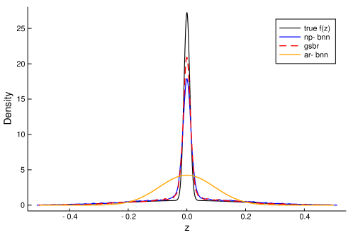
Figure 1: Kernel density estimator for the posterior predictive density based on the MCMC samples taken from NP-BNN (blue solid line), GSBR (red dashed line) and AR-BNN (orange solid line). The true density of the noise give in Equation (36) is superimposed with black color.

In Figure 1 we present the density of the noise component, that is, the 2-normal mixture given in Equation (36) (black solid line). Together we superimpose kernel density estimators (KDE) based on the posterior noise-predictive samples obtained from the NP-BNN (blue solid curve) and the GSBR model (Merkatas et al., 2017) (red solid line). The density of a Gaussian distribution with precision estimated from the AR-BNN (Nakada et al., 2005) with Gaussian noise is plotted in orange. For this heavy tailed distribution, as expected, models with nonparametric modeling of the noise components provide estimators nearly indistinguishable and very close to the true density. In contrast, the AR-BNN model overestimates the variance in order to capture the heavy tails and fails to estimate the intense peak of the mixture.

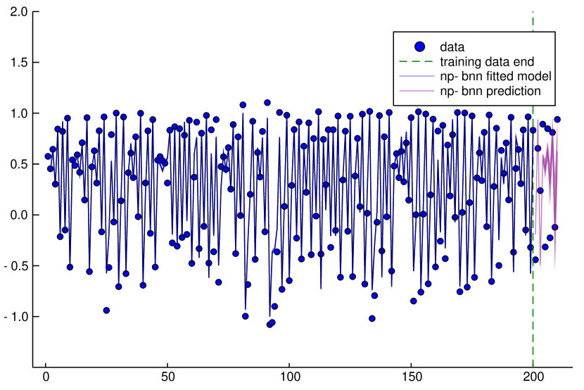
(a)

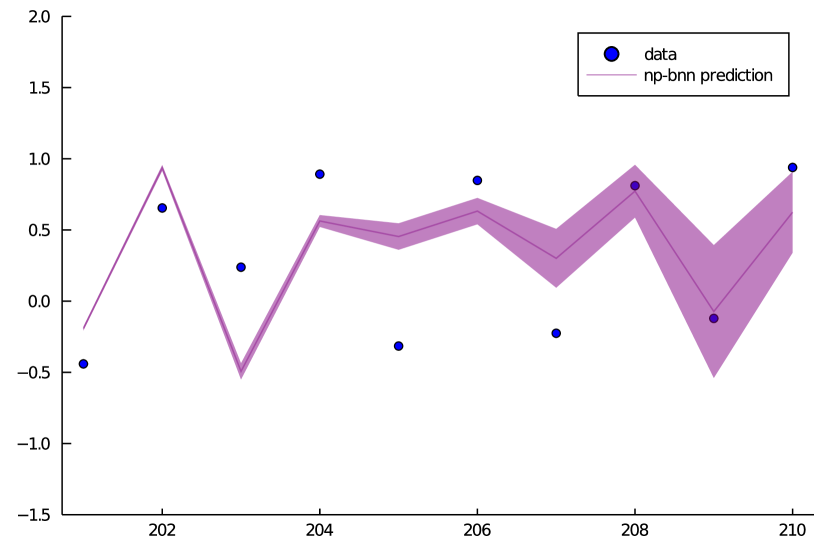
(b)

Figure 2: True time series generated from the noisy logistic map (blue dots) and the system identified from the proposed method (blue line) are shown in panel 2(a). The shaded lines represent sampling variability due to MCMC sampling. Additionally we present the predicted values for the future 10 values in purple. Panel 2(b) is a magnification of the prediction in time steps 201 to 210.

5.3. Real data: Canadian Lynx

As a real data example we take the Canadian Lynx data which consists of the annual trappings of lynx in the Mackenzie River District of North–West Canada for the period from 1821 to 1934 resulting to a total of 114 observations. We aim to identify the process responsible for the generation of the data using the first 100 observations and, additionally, test our model’s predictive capability on the last 14 observations.

As is common, we take the $\log_{10}$ transformation of the dataset. This data set has been widely used as a benchmark for nonlinear time series estimation and prediction before (Chan and Tong, 2001; Liang, 2005) and can be easily accessed from the web. The choice of lag is a model selection problem typically addressed using some information criterion like the Akaike information criterion (AIC) (Akaike, 1974). For an AR model, AIC chooses the best lag to be $\rho=11$ but, as in Liang (2005), we believe that this might lead to overfitting and we assume lag $\rho=2.$

For this example, we set the number of inputs in the neural net $N_{0}=2$. This corresponds to a autoregressive model with $\rho=2.$ Similar approach was taken also in Liang (2005). The base measure of the GSB process is chosen to be a gamma $\mathrm{Ga}(a_{\Lambda},b_{\Lambda})$ with $a=b=0.05.$ Here, we set $(\epsilon,S)=(0.005,20).$

The GSBR model is inappropriate for modeling real data, at least without first extending it to include the coefficients of a full quadratic model (Chan and Tong, 2001) so it is excluded from the comparison for fairness. We add in the comparison an AR model for which the best lag is $\rho=11$ according to AIC, and a feed forward neural network trained with backpropagation using the same number of hidden neurons and lagged values in the input layer. That is we choose 10 neurons and $\rho=2$ for straightforward comparisons.

In Figure 3 we present the ergodic means for the number of clusters estimated during the fitting process from which we conclude that the algorithm is mixing well and converges to the stationary distribution.

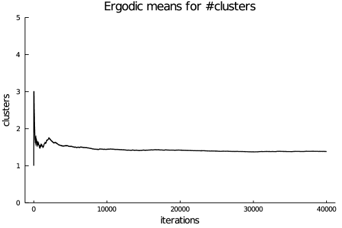
Figure 3: Ergodic means for the number of the active clusters during fitting.

In Figure 4 we represent the model fitted from the proposed method NP-BNN and the out of sample predictions for the next 14 values. The NP-BNN model outperforms all models in this comparison study with additional advantage that it can be used without any hypotheses about linearity of the time series or Gaussianity of its distribution. A comparison in terms of the evaluation metrics introduced in the beginning of this section is given in Table 2.

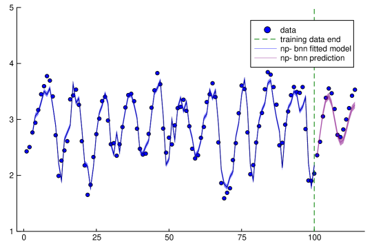
Figure 4: Fitted time series and 14-step ahead predictions for the Canadian Lynx data (blue dots). The blue line is the mean posterior function computed by the Bayesian neural network and the shaded blue lines represent the uncertainty associated with the function values based on sampled functions. In purple we represent the mean posterior prediction function for the 14 future observations with their associated uncertainties (purple-shaded lines).

Table 2: Evaluation metrics on Canadian Lynx data based on the prediction for the 14 future values. NP-BNN outperforms the models in the comparisons. For each model, the number in parentheses denotes the lag used for estimation.

Method	NP-BNN(2)	AR-BNN(2)	ANN(2)	AR(11)
MSE	0.0249	0.0897	0.0371	0.0822
RMSE	0.1579	0.2994	0.1926	0.2866
MAE	0.1350	0.2273	0.1487	0.2374
MAPE (%)	4.2727	6.9048	4.920	7.995
Theil’s $U$	0.0260	0.0502	0.0318	0.0476

6. Discussion

We have proposed an auto-regressive Bayesian neural network which assumes nonparametric noise process (NP-BNN) for the estimation and prediction of nonlinear time series models based on the assumption that the order of the underlying Markovian process is known. An MCMC sampler for posterior inference applicable in data sets with small sample size for which the noise process might depart from normality has been devised. In the limit of infinite neurons in the hidden layers, we have shown that this model converges to fully nonparametric Bayesian model enjoying all the flexibility of Gaussian process regression models without however, the need of matrix inversions, a characteristic that makes scaling of GPs difficult. Numerical results on simulated and real data sets indicate that the proposed model gives results comparable to the more traditional methods used for nonlinear time series modeling.

During modeling of dynamical phenomena, it is of special interest to estimate the initial state of the system additionally to the system parameters. It would be interesting to modify the proposed methodology so that a full conditional distribution for the initial unknown states when the process responsible for the generation of the time series is non-reversible. This however would require to invert the system $g$ which is not always feasible when $g$ is a neural network. To see this, consider for simplicity a prior $p(y_{0})=\mathbf{1}(-\zeta\leq y_{0}\leq\zeta)$ for the initial condition $y_{0}$ and for simplicity, a Gaussian noise model. Then under the proposed framework, the full conditional for $y_{0}$ reads

$$p(y_{0}\mid\cdots)\propto p(y_{0})\,\mathrm{N}(y_{1}\mid g(x_{0},\theta),\Lambda^{-1}).$$

To devise an exact algorithm based on Gibbs sampling, auxiliary variables can be introduced (Damlen et al., 1999) such that

$$p(y_{0},v_{0}\mid\cdots) \propto\mathbf{1}(-\zeta\leq y_{0}\leq\zeta)\,\exp\left\{-\frac{\Lambda}{2}v_{0}^{2}\right\}\,\mathbf{1}(v_{0}\geq\left(y_{1}-g(y_{0},\theta))^{2}\right).$$

The full conditional for the auxiliary $v_{0}$ is clearly a truncated exponential distribution. For $y_{0},$ one has to resort on solving the inequalities

$$p(y_{0}\mid v_{0}\cdots)\propto\mathbf{1}(-\zeta\leq y_{0}\leq\zeta)\,\mathbf{1}(y_{1}-\sqrt{v_{0}}\leq g(y_{0},\theta)\leq y_{1}+\sqrt{v_{0}}).$$

Letting

$$Z^{-}=\min\left\{-\zeta,g^{-1}\left(y_{1}-\sqrt{v_{0}},\theta\right)\right\},$$

and

$$Z^{+}=\max\left\{\zeta,g^{-1}\left(y_{1}+\sqrt{v_{0}},\theta\right)\right\},$$

the full conditional distribution for $x_{0}$ is given by

$$p(y_{0}\mid v_{0}\cdots)=\mathrm{U}\left(y_{0}\mid Z^{-},Z^{+}\right),$$

where $U$ denotes the uniform density. In this case a modeling approach would be to utilize normalizing flows as a model for $g$ which form a class of invertible neural networks (Rezende and Mohamed, 2015).

References

- Akaike (1974) Akaike, H. (1974). A new look at the statistical model identification. IEEE Transactions on Automatic Control, 19(6):716–723.
- Aladag et al. (2009) Aladag, C. H., Egrioglu, E., and Kadilar, C. (2009). Forecasting nonlinear time series with a hybrid methodology. Applied Mathematics Letters, 22(9):1467–1470.
- Antoniak (1974) Antoniak, C. E. (1974). Mixtures of Dirichlet processes with applications to Bayesian nonparametric problems. The Annals of Statistics, pages 1152–1174.
- Bijl et al. (2017) Bijl, H., Schön, T. B., van Wingerden, J.-W., and Verhaegen, M. (2017). System identification through online sparse Gaussian process regression with input noise. IFAC Journal of Systems and Control, 2:1–11.
- Box et al. (2015) Box, G. E., Jenkins, G. M., Reinsel, G. C., and Ljung, G. M. (2015). Time Series Analysis: Forecasting and Control. John Wiley & Sons.
- Brooks et al. (2011) Brooks, S., Gelman, A., Jones, G., and Meng, X.-L. (2011). Handbook of Markov Chain Monte Carlo. CRC Press.
- Carvalho et al. (2010) Carvalho, C. M., Polson, N. G., and Scott, J. G. (2010). The horseshoe estimator for sparse signals. Biometrika, 97(2):465–480.
- Chan and Tong (2001) Chan, K.-S. and Tong, H. (2001). Chaos: A Statistical Perspective. Springer Science & Business Media.
- Chen et al. (2018) Chen, R. T., Rubanova, Y., Bettencourt, J., and Duvenaud, D. (2018). Neural ordinary differential equations. In Neural Information Processing Systems, page 6571–6583.
- Chen and Billings (1992) Chen, S. and Billings, S. (1992). Neural networks for nonlinear dynamic system modeling and identification. International Journal of Control, 56(2):319–346.
- Cybenko (1989) Cybenko, G. (1989). Approximation by superpositions of a sigmoidal function. Mathematics of Control, Signals and Systems, 2(4):303–314.
- Damlen et al. (1999) Damlen, P., Wakefield, J., and Walker, S. (1999). Gibbs sampling for Bayesian non-conjugate and hierarchical models by using auxiliary variables. Journal of the Royal Statistical Society: Series B (Statistical Methodology), 61(2):331–344.
- De Blasi et al. (2020) De Blasi, P., Martínez, A. F., Mena, R. H., and Prünster, I. (2020). On the inferential implications of decreasing weight structures in mixture models. Computational Statistics & Data Analysis, 147:106940.
- Engle (1982) Engle, R. F. (1982). Autoregressive conditional heteroscedasticity with estimates of the variance of United Kingdom inflation. Econometrica: Journal of the Econometric Society, pages 987–1007.
- Escobar and West (1995) Escobar, M. D. and West, M. (1995). Bayesian density estimation and inference using mixtures. Journal of the American Statistical Association, 90(430):577–588.
- Ferguson (1973) Ferguson, T. S. (1973). A Bayesian analysis of some nonparametric problems. The Annals of Statistics, pages 209–230.
- Fermanian (2021) Fermanian, A. (2021). Embedding and learning with signatures. Computational Statistics & Data Analysis, 157:107148.
- Franses et al. (2000) Franses, P. H., Van Dijk, D., et al. (2000). Non-linear Time Series Models in Empirical Finance. Cambridge University Press.
- Fuentes-García et al. (2009) Fuentes-García, R., Mena, R. H., and Walker, S. G. (2009). A nonparametric dependent process for Bayesian regression. Statistics & Probability Letters, 79(8):1112–1119.
- Fuentes-Garcia et al. (2010) Fuentes-Garcia, R., Mena, R. H., and Walker, S. G. (2010). A new Bayesian nonparametric mixture model. Communications in Statistics—Simulation and Computation®, 39(4):669–682.
- Gelman et al. (2013) Gelman, A., Carlin, J. B., Stern, H. S., Dunson, D. B., Vehtari, A., and Rubin, D. B. (2013). Bayesian Data Analysis. CRC Press.
- Geman and Geman (1984) Geman, S. and Geman, D. (1984). Stochastic relaxation, Gibbs distributions, and the Bayesian restoration of images. IEEE Transactions on Pattern Analysis and Machine Intelligence, PAMI-6(6):721–741.
- Ghosal and Van der Vaart (2017) Ghosal, S. and Van der Vaart, A. (2017). Fundamentals of nonparametric Bayesian inference, volume 44. Cambridge University Press.
- Goodfellow et al. (2016) Goodfellow, I., Bengio, Y., and Courville, A. (2016). Deep Learning. MIT Press.
- Hatjispyros and Merkatas (2019) Hatjispyros, S. J. and Merkatas, C. (2019). Joint reconstruction and prediction of random dynamical systems under borrowing of strength. Chaos: An Interdisciplinary Journal of Nonlinear Science, 29(2):023121.
- Hatjispyros et al. (2018) Hatjispyros, S. J., Merkatas, C., Nicoleris, T., and Walker, S. G. (2018). Dependent mixtures of geometric weights priors. Computational Statistics & Data Analysis, 119:1–18.
- Hatjispyros et al. (2009) Hatjispyros, S. J., Nicoleris, T., and Walker, S. G. (2009). A Bayesian nonparametric study of a dynamic nonlinear model. Computational Statistics & Data Analysis, 53(12):3948–3956.
- Hjort et al. (2010) Hjort, N. L., Holmes, C., Müller, P., and Walker, S. G. (2010). Bayesian Nonparametrics, volume 28. Cambridge University Press.
- Ishwaran and James (2001) Ishwaran, H. and James, L. F. (2001). Gibbs sampling methods for stick-breaking priors. Journal of the American Statistical Association, 96(453):161–173.
- Ishwaran and Rao (2005) Ishwaran, H. and Rao, J. S. (2005). Spike and slab variable selection: frequentist and Bayesian strategies. The Annals of Statistics, 33(2):730–773.
- Kalli et al. (2011) Kalli, M., Griffin, J. E., and Walker, S. G. (2011). Slice sampling mixture models. Statistics and computing, 21(1):93–105.
- Keesman (2011) Keesman, K. J. (2011). System Identification: an Introduction. Springer Science & Business Media.
- Kennedy (1988) Kennedy, A. (1988). Hybrid Monte Carlo. Nuclear Physics B-Proceedings Supplements, 4:576–579.
- Kocijan et al. (2005) Kocijan, J., Girard, A., Banko, B., and Murray-Smith, R. (2005). Dynamic systems identification with Gaussian processes. Mathematical and Computer Modelling of Dynamical Systems, 11(4):411–424.
- Lau and Tse (2003) Lau, F. and Tse, C. (2003). Chaos-Based Digital Communication Systems. Springer-Verlag.
- Liang (2005) Liang, F. (2005). Bayesian neural networks for nonlinear time series forecasting. Statistics and Computing, 15(1):13–29.
- Lijoi et al. (2014) Lijoi, A., Nipoti, B., and Prünster, I. (2014). Dependent mixture models: clustering and borrowing information. Computational Statistics & Data Analysis, 71:417–433.
- Ljung (1999) Ljung, L. (1999). System Identification: Theory for the User, 2nd Edition. Prentice-Hall Inc., Englewood Cliffs, NJ.
- Luengo et al. (2002) Luengo, D., Pantaleón, C., and Santamaría, I. (2002). Bayesian estimation of discrete chaotic signals by MCMC. In 2002 11th European Signal Processing Conference, pages 1–4. IEEE.
- MacKay (1992) MacKay, D. J. (1992). A practical Bayesian framework for backpropagation networks. Neural Computation, 4(3):448–472.
- Matsumoto et al. (2001) Matsumoto, T., Nakajima, Y., Saito, M., Sugi, J., and Hamagishi, H. (2001). Reconstructions and predictions of nonlinear dynamical systems: A hierarchical Bayesian approach. IEEE Transactions on Signal Srocessing, 49(9):2138–2155.
- Mena et al. (2011) Mena, R. H., Ruggiero, M., and Walker, S. G. (2011). Geometric stick-breaking processes for continuous-time Bayesian nonparametric modeling. Journal of Statistical Planning and Inference, 141(9):3217–3230.
- Merkatas et al. (2017) Merkatas, C., Kaloudis, K., and Hatjispyros, S. J. (2017). A Bayesian nonparametric approach to reconstruction and prediction of random dynamical systems. Chaos: An Interdisciplinary Journal of Nonlinear Science, 27(6):063116.
- Meyer and Christensen (2000) Meyer, R. and Christensen, N. (2000). Bayesian reconstruction of chaotic dynamical systems. Physical Review E, 62(3):3535.
- Nakada et al. (2005) Nakada, Y., Matsumoto, T., Kurihara, T., and Yosui, K. (2005). Bayesian reconstructions and predictions of nonlinear dynamical systems via the hybrid Monte Carlo scheme. Signal Processing, 85(1):129–145.
- Neal (1996) Neal, R. M. (1996). Bayesian Learning for Neural Networks, volume 118. Springer Science & Business Media.
- Neal et al. (2011) Neal, R. M. et al. (2011). MCMC using Hamiltonian dynamics. In Brooks, S., Gelman, A., Jones, G. L., and Meng, X.-L., editors, Handbook of Markov Chain Monte Carlo, chapter 5. Chapman & Hall/CRC.
- Nelles (2001) Nelles, O. (2001). Nonlinear dynamic system identification. In Nonlinear System Identification: From Classical Approaches to Neural Networks and Fuzzy Models, chapter 17, pages 547–577. Springer.
- Nowlan and Hinton (1992) Nowlan, S. J. and Hinton, G. E. (1992). Simplifying neural networks by soft weight-sharing. Neural Computation, 4(4):473–493.
- Ongaro and Cattaneo (2004) Ongaro, A. and Cattaneo, C. (2004). Discrete random probability measures: a general framework for nonparametric Bayesian inference. Statistics & Probability Letters, 67(1):33–45.
- Ozaki (2012) Ozaki, T. (2012). Time Series Modeling of Neuroscience Data. CRC press.
- Pantaleón et al. (2000) Pantaleón, C., Luengo, D., and Santamaria, I. (2000). Bayesian estimation of a class of chaotic signals. In Proceedings of IEEE International Conference on Acoustics, Speech, and Signal Processing, volume 1, pages 193–196. IEEE.
- Pantaleón et al. (2003) Pantaleón, C., Vielva, L., Luengo, D., and Santamarı’a, I. (2003). Bayesian estimation of chaotic signals generated by piecewise-linear maps. Signal Processing, 83(3):659–664.
- Pindyck and Rubinfeld (1998) Pindyck, S. and Rubinfeld, L. (1998). Econometric Models and Economic Forecasts. McGraw-Hill.
- Polson and Scott (2010) Polson, N. G. and Scott, J. G. (2010). Shrink globally, act locally: Sparse Bayesian regularization and prediction. Bayesian statistics, 9(501-538):105.
- Rasmussen and Williams (2006) Rasmussen, C. E. and Williams, C. K. I. (2006). Gaussian Processes for Machine Learning. Adaptive computation and machine learning. MIT Press.
- Rezende and Mohamed (2015) Rezende, D. and Mohamed, S. (2015). Variational inference with normalizing flows. In International Conference on Machine Learning, pages 1530–1538. PMLR.
- Särkkä et al. (2018) Särkkä, S., Álvarez, M. A., and Lawrence, N. D. (2018). Gaussian process latent force models for learning and stochastic control of physical systems. IEEE Transactions on Automatic Control, 64(7):2953–2960.
- Sethuraman (1994) Sethuraman, J. (1994). A constructive definition of Dirichlet priors. Statistica Sinica, pages 639–650.
- Sjöberg et al. (1994) Sjöberg, J., Hjalmarsson, H., and Ljung, L. (1994). Neural networks in system identification. IFAC Proceedings, 27(8):359–382.
- Sjöberg et al. (1995) Sjöberg, J., Zhang, Q., Ljung, L., Benveniste, A., Delyon, B., Glorennec, P.-Y., Hjalmarsson, H., and Juditsky, A. (1995). Nonlinear black-box modeling in system identification: a unified overview. Automatica, 31(12):1691–1724.
- Small (2005) Small, M. (2005). Applied Nonlinear Time Series analysis: Applications in Physics, Physiology and Finance, volume 52. World Scientific.
- Tong and Lim (1980) Tong, H. and Lim, K. (1980). Threshold autoregression, limit cycles and cyclidal data. Journal of the Royal Statistical Society: Series B (Statistical Methodology), 43(12):245–292.
- Turner et al. (2009) Turner, R., Deisenroth, M. P., and Rasmussen, C. E. (2009). System identification in Gaussian process dynamical systems. In Nonparametric Bayes Workshop (NIPS 2009), Whistler, BC, Canada.
- Walker (2007) Walker, S. G. (2007). Sampling the Dirichlet mixture model with slices. Communications in Statistics—Simulation and Computation®, 36(1):45–54.
- Zhang (2003) Zhang, G. P. (2003). Time series forecasting using a hybrid ARIMA and neural network model. Neurocomputing, 50:159–175.