Abstract

In the article, we investigate the diquark-diquark-antiquark type fully-heavy pentaquark states with the spin-parity $J^{P}={\frac{1}{2}}^{-}$ via the QCD sum rules for the first time, and obtain the masses $M_{cccc\bar{c}}=7.93\pm 0.15\,\rm{GeV}$ and $M_{bbbb\bar{b}}=23.91\pm 0.15\,\rm{GeV}$. We can search for the fully-heavy pentaquark states in the $J/\psi\Omega_{ccc}$ and $\Upsilon\Omega_{bbb}$ invariant mass spectrum in the future.

PACS number: 12.39.Mk, 12.38.Lg

Key words: Fully-heavy pentaquark states, QCD sum rules

1 Introduction

In the quark models, we usually classify the hadrons into the traditional quark-antiquark type mesons, three-quark baryons, and exotic states, such as the tetraquark (molecular) states, pentaquark (molecular) states and hexaquark (molecular) states, etc. The tetraquark (molecular) states are also referred to as mesons due to their integer spins. A number of exotic states have been observed in recent years, such as the $X(3860)$, $X(3872)$, $Z_{c}(3885/3900)$, $X(3915)$, $X(3940)$, $Z_{c}(4020/4025)$, $Z_{c}(4050)$, $Z_{c}(4055)$, $Z_{c}(4100)$, $X(4160)$, $Z_{c}(4200)$, $Y(4220)$, $Y(4260)$, $Z_{c}(4250)$, $Y(4320)$, $Y(4360)$, $Y(4390)$, $Z_{c}(4430)$, $Z_{c}(4600)$, $Y(4660)$, etc [1, 2]. The most illusive meson $X(3872)$ has hidden-charm, but cannot be assigned to be any radial or orbital excited state of the charmonium, and should have more complicated inner quark structures than a mere $c\bar{c}$ pair [3]. The exotic states provide us with a unique subject to investigate the strong interaction, which governs the dynamics of the quarks and gluons, and the confinement mechanism. If those exotic $X$, $Y$, $Z$ states are genuine tetraquark (molecular) states, there are two heavy valence quarks and two light valence quarks, we have to deal with the complex dynamics involving both the heavy and light degrees of freedom.

In 2017, the LHCb collaboration observed the doubly-charmed baryon state $\Xi_{cc}^{++}$ [4], which provides us with the crucial experimental input on the strong correlation between the two charm (or two heavy) quarks, and is of great importance on the spectroscopy of the fully-heavy baryon states and multiquark states. However, just like in the case of the exotic $X$, $Y$, $Z$ states, we also have to deal with the complex dynamics involving both the heavy and light degrees of freedom. Moreover, only the doubly-charmed baryon state $\Xi_{cc}^{++}$ is observed up to now, other doubly-heavy baryon states and triply-heavy baryon states still escape from experimental detecting.

In 2020, the LHCb collaboration observed a narrow structure $X(6900)$ and a broad structure just above the $J/\psi J/\psi$ threshold in the $J/\psi J/\psi$ invariant mass spectrum [5], such structures are the first fully-heavy exotic multiquark candidates claimed experimentally up to now. It is a very important step in investigations of the heavy hadrons, and provides very important experimental constraints on the theoretical models. The fully-heavy tetraquark candidate $X(6900)$ was observed before observation of the fully-heavy baryon state $\Omega_{ccc}$.

The attractive interaction induced by one-gluon exchange favors formation of the diquarks in color antitriplet, which are the basic building blocks of the diquark-antidiquark type tetraquark states [6, 7]. Fermi-Dirac statistics requires $\varepsilon^{abc}Q^{T}_{b}C\Gamma Q_{c}=\varepsilon^{abc}Q^{T}_{b}\left[C\Gamma\right]^{T}Q_{c}$, $\left[C\Gamma\right]^{T}=-C\Gamma$ for $\Gamma=\gamma_{5}$, $1$, $\gamma_{\mu}\gamma_{5}$, $\left[C\Gamma\right]^{T}=C\Gamma$ for $\Gamma=\gamma_{\mu}$, $\sigma_{\mu\nu}$, only the axialvector diquarks $\varepsilon^{abc}Q^{T}_{b}C\gamma_{\mu}Q_{c}$ and tensor diquarks $\varepsilon^{abc}Q^{T}_{b}C\sigma_{\mu\nu}Q_{c}$ can exist, where the $a$, $b$ and $c$ are color indexes. Under parity transform $\widehat{P}$, the diquarks $\varepsilon^{abc}Q^{T}_{b}C\gamma_{\mu}Q_{c}$ and $\varepsilon^{abc}Q^{T}_{b}C\sigma_{\mu\nu}Q_{c}$ have the properties $\varepsilon^{abc}Q^{T}_{b}C\gamma_{\mu}Q_{c}\widehat{P}^{-1}=-\varepsilon^{abc}Q^{T}_{b}C\gamma^{\mu}Q_{c}$ and $\widehat{P}\varepsilon^{abc}Q^{T}_{b}C\sigma_{\mu\nu}Q_{c}\widehat{P}^{-1}=-\varepsilon^{abc}Q^{T}_{b}C\sigma^{\mu\nu}Q_{c}$, respectively, so we usually refer to them as the axialvector and tensor diquarks, respectively. The diquarks $\varepsilon^{abc}Q^{T}_{b}C\sigma_{\mu\nu}Q_{c}$ have both the $J^{P}=1^{+}$ and $1^{-}$ components, for the $J^{P}=1^{-}$ component, there exists an implicit P-wave which is embodied in the negative parity, the axialvector diquarks $\varepsilon^{abc}Q^{T}_{b}C\gamma_{\mu}Q_{c}$ are more stable than the tensor diquarks $\varepsilon^{abc}Q^{T}_{b}C\sigma_{\mu\nu}Q_{c}$ due to the additional energy excited by the P-wave, we usually take the axialvector diquarks $\varepsilon^{abc}Q^{T}_{b}C\gamma_{\mu}Q_{c}$ as the basic building blocks to investigate doubly-heavy baryon states, tetraquark states and pentaquark states [8, 9, 10, 11].

We can introduce an explicit P-wave to construct the doubly-heavy diquarks $\varepsilon^{abc}Q^{T}_{b}C\gamma_{5}\stackrel{{\scriptstyle\leftrightarrow}}{{\partial}}_{\mu}Q_{c}$, $\varepsilon^{abc}Q^{T}_{b}C\gamma_{5}\underline{\gamma_{5}}\stackrel{{\scriptstyle\leftrightarrow}}{{\partial}}_{\mu}Q_{c}$, $\varepsilon^{abc}Q^{T}_{b}C\gamma_{\alpha}\underline{\gamma_{5}}\stackrel{{\scriptstyle\leftrightarrow}}{{\partial}}_{\mu}Q_{c}$, which can exist due to the Fermi-Dirac statistics, there are two-type P-waves, the explicit P-wave is embodied in the derivative $\stackrel{{\scriptstyle\leftrightarrow}}{{\partial}}_{\mu}=\stackrel{{\scriptstyle\rightarrow}}{{\partial}}_{\mu}-\stackrel{{\scriptstyle\leftarrow}}{{\partial}}_{\mu}$, while the implicit P-wave is embodied in the underlined $\underline{\gamma_{5}}$, as multiplying $\gamma_{5}$ to the diquarks changes their parity. The $\varepsilon^{abc}Q^{T}_{b}C\gamma_{5}\stackrel{{\scriptstyle\leftrightarrow}}{{\partial}}_{\mu}Q_{c}$ are P-wave diquarks, while the $\varepsilon^{abc}Q^{T}_{b}C\gamma_{5}\underline{\gamma_{5}}\stackrel{{\scriptstyle\leftrightarrow}}{{\partial}}_{\mu}Q_{c}$ and $\varepsilon^{abc}Q^{T}_{b}C\gamma_{\alpha}\underline{\gamma_{5}}\stackrel{{\scriptstyle\leftrightarrow}}{{\partial}}_{\mu}Q_{c}$ are D-wave diquarks. We can also introduce an explicit D-wave $\stackrel{{\scriptstyle\leftrightarrow}}{{\partial}}_{\mu}\stackrel{{\scriptstyle\leftrightarrow}}{{\partial}}_{\nu}$ to construct the doubly-heavy diquarks, for example, $\varepsilon^{abc}Q^{T}_{b}C\gamma_{\alpha}\stackrel{{\scriptstyle\leftrightarrow}}{{\partial}}_{\mu}\stackrel{{\scriptstyle\leftrightarrow}}{{\partial}}_{\nu}Q_{c}$. If we take those P-wave and D-wave diquarks as the basic building blocks to investigate the doubly-heavy baryon states, tetraquark states and pentaquark states, we expect to obtain larger hadron masses considering the additional contributions from the P-waves and D-wave.

In 2015, the LHCb collaboration observed the pentaquark candidates $P_{c}(4380)$ and $P_{c}(4450)$ in the $J/\psi p$ mass spectrum in the $\Lambda_{b}^{0}\to J/\psi K^{-}p$ decays [12]. In 2019, the LHCb collaboration observed a narrow pentaquark candidate $P_{c}(4312)$ and proved that the $P_{c}(4450)$ consists of two overlapping narrow structures $P_{c}(4440)$ and $P_{c}(4457)$ [13]. In 2020, the LHCb collaboration observed the first evidence of a hidden-charm pentaquark candidate $P_{cs}(4459)$ with strangeness in the $J/\psi\Lambda$ mass spectrum in the $\Xi_{b}^{-}\to J/\psi K^{-}\Lambda$ decays [14]. They are all very good candidates for the hidden-charm pentaquark (molecular) states [15, 16, 17]. In this case, we also have to deal with the complex dynamics involving both the heavy and light degrees of freedom.

Analogously, we expect to observe the fully-heavy pentaquark candidates $QQQQ\bar{Q}$ in the $J/\psi\Omega_{ccc}$ and $\Upsilon\Omega_{bbb}$ invariant mass spectrum at the LHCb, CEPC, FCC and ILC in the future. Theoretically, J. R. Zhang explores the $\eta_{c}\Omega_{ccc}$ and $\eta_{b}\Omega_{bbb}$ pentaquark molecular states with the QCD sum rules [18]. H. T. An et al explore the fully-heavy pentaquark states in the framework of the modified chromo-magnetic interaction model [19].

In the present work, we construct the diquark-diquark-antiquark type five-quark currents to interpolate the fully-heavy pentaquark states with the same flavor via the QCD sum rules, and make predictions to be confronted to the experimental data in the future, as the QCD sum rules is a powerful theoretical tool in investigating the exotic $X$, $Y$, $Z$ and $P$ states [20].

The article is arranged as follows: we derive the QCD sum rules for the masses and pole residues of the fully-heavy pentaquark states in section 2; in section 3, we present the numerical results and discussions; section 4 is reserved for our conclusion.

2 QCD sum rules for the fully-heavy pentaquark states

Let us write down the correlation functions $\Pi(p)$,

$$\Pi(p) = i\int d^{4}xe^{ip\cdot x}\langle 0|T\left\{J(x)\bar{J}(0)\right\}|0\rangle\,,$$ (1)

where

$$J(x) = \varepsilon^{ajk}\varepsilon^{bmn}\varepsilon^{abc}Q^{T}_{j}(x)C\gamma_{\mu}Q_{k}(x)\,Q^{T}_{m}(x)C\gamma_{\nu}Q_{n}(x)\,\sigma^{\mu\nu}C\bar{Q}^{T}_{c}(x)\,,$$ (2)

$Q=b$, $c$, the $a$, $b$, $c$, $j$, $k$, $m$, $n$ are color indexes. We can construct other five-quark currents with the same flavor to interpolate the fully-heavy pentaquark states, for example,

$$\eta(x) = \varepsilon^{ajk}\varepsilon^{bmn}\varepsilon^{abc}Q^{T}_{j}(x)C\sigma_{\mu\alpha}Q_{k}(x)\,Q^{T}_{m}(x)C\sigma^{\mu}{}_{\beta}Q_{n}(x)\,\sigma^{\alpha\beta}C\bar{Q}^{T}_{c}(x)\,,$$

$$\eta_{\mu}(x) = \varepsilon^{ajk}\varepsilon^{bmn}\varepsilon^{abc}Q^{T}_{j}(x)C\sigma_{\mu\alpha}Q_{k}(x)\,Q^{T}_{m}(x)C\gamma^{\alpha}Q_{n}(x)\,C\bar{Q}^{T}_{c}(x)\,,$$

$$\eta_{\mu\nu}(x) = \varepsilon^{ajk}\varepsilon^{bmn}\varepsilon^{abc}Q^{T}_{j}(x)C\sigma_{\mu\alpha}Q_{k}(x)\,Q^{T}_{m}(x)C\sigma_{\nu\beta}Q_{n}(x)\,\sigma^{\alpha\beta}C\bar{Q}^{T}_{c}(x)\,.$$ (3)

As the axialvector diquarks $\varepsilon^{ijk}Q^{T}_{j}C\gamma_{\mu}Q_{k}$ are more stable than the tensor diquarks $\varepsilon^{ijk}Q^{T}_{j}C\sigma_{\mu\nu}Q_{k}$, we choose the currents $J(x)$ to investigate the lowest fully-heavy pentaquark states.

Under parity transform $\widehat{P}$, the currents $J(x)$ have the property,

$$\widehat{P}J(x)\widehat{P}^{-1} = -\gamma^{0}J(\tilde{x})\,,$$ (4)

where $x^{\mu}=(t,\vec{x})$ and $\tilde{x}^{\mu}=(t,-\vec{x})$. The currents $J(x)$ have negative parity, and couple potentially to the fully-heavy pentaquark states with the spin-parity $J^{P}={\frac{1}{2}}^{-}$,

$$\langle 0|J(0)|P^{-}(p)\rangle = \lambda_{-}U^{-}(p,s)\,,$$ (5)

where the $\lambda_{-}$ are the pole residues and the $U^{-}(p,s)$ are the Dirac spinors. However, they also couple potentially to the fully-heavy pentaquark states with the spin-parity $J^{P}={\frac{1}{2}}^{+}$, because multiplying $i\gamma_{5}$ to the currents $J(x)$ changes their parity,

$$\langle 0|J(0)|P^{+}(p)\rangle = \lambda_{+}i\gamma_{5}U^{+}(p,s)\,,$$ (6)

again the $\lambda_{+}$ are the pole residues and the $U^{+}(p,s)$ are the Dirac spinors.

At the hadron side, we isolate the pole terms of the lowest fully-heavy pentaquark states with negative parity and positive parity together, and obtain the results:

$$\Pi(p) = \lambda^{2}_{-}{\!\not\!{p}+M_{-}\over M_{-}^{2}-p^{2}}+\lambda^{2}_{+}{\!\not\!{p}-M_{+}\over M_{+}^{2}-p^{2}}+\cdots\,,$$ (7)

$$= \Pi_{1}(p^{2})\!\not\!{p}+\Pi_{0}(p^{2})\,.$$

Then we obtain the hadronic spectral densities through dispersion relation,

$$\frac{{\rm Im}\Pi_{1}(s)}{\pi} = \lambda^{2}_{-}\delta\left(s-M_{-}^{2}\right)+\lambda^{2}_{+}\delta\left(s-M_{+}^{2}\right)=\,\rho_{1,H}(s)\,,$$ (8)

$$\frac{{\rm Im}\Pi_{0}(s)}{\pi} = M_{-}\lambda^{2}_{-}\delta\left(s-M_{-}^{2}\right)-M_{+}\lambda_{+}^{2}\delta\left(s-M_{+}^{2}\right)=\rho_{0,H}(s)\,,$$ (9)

where we add the subscript $H$ to represent the hadron side. We introduce the weight functions $\sqrt{s}\exp\left(-\frac{s}{T^{2}}\right)$ and $\exp\left(-\frac{s}{T^{2}}\right)$ to acquire the QCD sum rules at the hadron side,

$$\int_{25m_{Q}^{2}}^{s_{0}}ds\left[\sqrt{s}\,\rho_{1,H}(s)+\rho_{0,H}(s)\right]\exp\left(-\frac{s}{T^{2}}\right) = 2M_{-}\lambda^{2}_{-}\exp\left(-\frac{M_{-}^{2}}{T^{2}}\right)\,,$$ (10)

where the $s_{0}$ are the continuum threshold parameters, the $T^{2}$ are the Borel parameters, there are no contaminations from the fully-heavy pentaquark states with the positive parity due to the special combination.

In accomplishing the tedious and terrible operator product expansion, we take account of the gluon condensate and neglect the three-gluon condensate. After we obtain the spectral densities at the quark-gluon level, we match the hadron side with the QCD side of the correlation functions $\Pi(p)$, again we introduce the weight functions $\sqrt{s}\exp\left(-\frac{s}{T^{2}}\right)$ and $\exp\left(-\frac{s}{T^{2}}\right)$ to obtain the QCD sum rules:

$$2M_{-}\lambda_{-}^{2}\exp\left(-\frac{M_{-}^{2}}{T^{2}}\right) = \int_{25m_{Q}^{2}}^{s_{0}}ds\int_{16m_{Q}^{2}}^{(\sqrt{s}-m_{Q})^{2}}dr\int_{4m_{Q}^{2}}^{(\sqrt{r}-2m_{Q})^{2}}dt_{1}\int_{4m_{Q}^{2}}^{(\sqrt{r}-\sqrt{t_{1}})^{2}}dt_{2}$$ (11)

$$\rho_{QCD}(s,r,t_{1},t_{2})\exp\left(-\frac{s}{T^{2}}\right)\,,$$

where $\rho_{QCD}(s,r,t_{1},t_{2})=\sqrt{s}\rho_{1,QCD}+\rho_{0,QCD}$, $\rho_{0,QCD}=m_{Q}\widetilde{\rho}_{0,QCD}$,

$$\rho_{1,QCD} = \frac{1}{2304\pi^{8}}\frac{\sqrt{\lambda(s,r,m_{Q}^{2})}}{s}\frac{\sqrt{\lambda(r,t_{1},t_{2})}}{r}\frac{\sqrt{\lambda(t_{1},m_{Q}^{2},m_{Q}^{2})}}{t_{1}}\frac{\sqrt{\lambda(t_{2},m_{Q}^{2},m_{Q}^{2})}}{t_{2}}$$ (12)

$$\left(C_{1,8}m_{Q}^{8}+C_{1,6}m_{Q}^{6}+C_{1,4}m_{Q}^{4}+C_{1,2}m_{Q}^{2}+C_{1,0}\right)$$

$$+\frac{1}{864\pi^{6}}\langle\frac{\alpha_{s}GG}{\pi}\rangle\frac{1}{s^{2}\sqrt{\lambda(s,r,m_{Q}^{2})}^{5}}\frac{\sqrt{\lambda(r,t_{1},t_{2})}}{r}\frac{\sqrt{\lambda(t_{1},m_{Q}^{2},m_{Q}^{2})}}{t_{1}}\frac{\sqrt{\lambda(t_{2},m_{Q}^{2},m_{Q}^{2})}}{t_{2}}$$

$$\left(C_{1,16}^{A}m_{Q}^{16}+C_{1,14}^{A}m_{Q}^{14}+C_{1,12}^{A}m_{Q}^{12}+C_{1,10}^{A}m_{Q}^{10}+C_{1,8}^{A}m_{Q}^{8}+C_{1,6}^{A}m_{Q}^{6}+C_{1,4}^{A}m_{Q}^{4}+C_{1,2}^{A}m_{Q}^{2}\right)$$

$$+\frac{1}{13824\pi^{6}}\langle\frac{\alpha_{s}GG}{\pi}\rangle\frac{\sqrt{\lambda(s,r,m_{Q}^{2})}}{s}\frac{\sqrt{\lambda(r,t_{1},t_{2})}}{r}\frac{1}{t_{1}\sqrt{\lambda(t_{1},m_{Q}^{2},m_{Q}^{2})}^{3}}\frac{\sqrt{\lambda(t_{2},m_{Q}^{2},m_{Q}^{2})}}{t_{2}}$$

$$\left(C_{1,10}^{B}m_{Q}^{10}+C_{1,8}^{B}m_{Q}^{8}+C_{1,6}^{B}m_{Q}^{6}+C_{1,4}^{B}m_{Q}^{4}+C_{1,2}^{B}m_{Q}^{2}\right)\,,$$

$$\widetilde{\rho}_{0,QCD} = \frac{1}{1152\pi^{8}}\frac{\sqrt{\lambda(s,r,m_{Q}^{2})}}{s}\frac{\sqrt{\lambda(r,t_{1},t_{2})}}{r}\frac{\sqrt{\lambda(t_{1},m_{Q}^{2},m_{Q}^{2})}}{t_{1}}\frac{\sqrt{\lambda(t_{2},m_{Q}^{2},m_{Q}^{2})}}{t_{2}}$$ (13)

$$\left(C_{0,4}m_{Q}^{4}+C_{0,2}m_{Q}^{2}+C_{0,0}\right)$$

$$+\frac{1}{1152\pi^{6}}\langle\frac{\alpha_{s}GG}{\pi}\rangle\frac{1}{\sqrt{\lambda(s,r,m_{Q}^{2})}^{5}}\frac{\sqrt{\lambda(r,t_{1},t_{2})}}{r}\frac{\sqrt{\lambda(t_{1},m_{Q}^{2},m_{Q}^{2})}}{t_{1}}\frac{\sqrt{\lambda(t_{2},m_{Q}^{2},m_{Q}^{2})}}{t_{2}}$$

$$\left(C_{0,6}^{A}m_{Q}^{6}+C_{0,4}^{A}m_{Q}^{4}+C_{0,2}^{A}m_{Q}^{2}+C_{0,0}^{A}\right)$$

$$+\frac{1}{13824\pi^{6}}\langle\frac{\alpha_{s}GG}{\pi}\rangle\frac{\sqrt{\lambda(s,r,m_{Q}^{2})}}{s}\frac{\sqrt{\lambda(r,t_{1},t_{2})}}{r}\frac{1}{t_{1}\sqrt{\lambda(t_{1},m_{Q}^{2},m_{Q}^{2})}^{3}}\frac{\sqrt{\lambda(t_{2},m_{Q}^{2},m_{Q}^{2})}}{t_{2}}$$

$$\left(C_{0,6}^{B}m_{Q}^{6}+C_{0,4}^{B}m_{Q}^{4}+C_{0,2}^{B}m_{Q}^{2}+C_{0,0}^{B}\right)\,,$$

where

$$C_{1,8} = \frac{24}{{s}{r}}-\frac{16({t_{1}}+{t_{2}})}{sr^{2}}+\frac{4r}{st_{1}t_{2}}+\frac{8}{s}\left(\frac{1}{t_{1}}+\frac{1}{t_{2}}\right)-\frac{28}{{s}{r}}\left(\frac{t_{1}}{t_{2}}+\frac{t_{2}}{t_{1}}\right)+\frac{16}{sr^{2}}\left(\frac{t_{1}^{2}}{t_{2}}+\frac{t_{2}^{2}}{t_{1}}\right)\,,$$

$$C_{1,6} = -\frac{4}{s}+\frac{6({t_{1}}+{t_{2}})}{{s}{r}}-\frac{16{t_{1}}{t_{2}}}{sr^{2}}+\frac{32({t_{1}}+{t_{2}})-48r}{r^{2}}-\frac{8r}{t_{1}t_{2}}-\frac{2r^{2}}{st_{1}t_{2}}-\left(16+\frac{2r}{s}\right)\left(\frac{1}{t_{1}}+\frac{1}{t_{2}}\right)$$

$$+\left(\frac{18}{s}+\frac{56}{r}\right)\left(\frac{t_{1}}{t_{2}}+\frac{t_{2}}{t_{1}}\right)-\left(\frac{22}{{s}{r}}+\frac{32}{r^{2}}\right)\left(\frac{t_{1}^{2}}{t_{2}}+\frac{t_{2}^{2}}{t_{1}}\right)+\frac{8}{sr^{2}}\left(\frac{t_{1}^{3}}{t_{2}}+\frac{t_{2}^{3}}{t_{1}}\right)\,,$$

$$C_{1,4} = -28+\frac{11(t_{1}+t_{2})}{s}-\frac{15r}{s}+\frac{24s^{2}+12s(t_{1}+t_{2})-7(t_{1}-t_{2})^{2}}{{s}{r}}+\frac{4sr-2r^{2}}{t_{1}t_{2}}-\frac{2r^{3}}{st_{1}t_{2}}$$

$$+\frac{4\left[t_{1}^{3}+t_{2}^{3}-t_{1}t_{2}(t_{1}+t_{2})-4s^{2}(t_{1}+t_{2})+8st_{1}t_{2}\right]}{sr^{2}}+\left(8s-8r-\frac{5r^{2}}{s}\right)\left(\frac{1}{t_{1}}+\frac{1}{t_{2}}\right)$$

$$+\left(6+\frac{12r}{s}-\frac{28s}{r}\right)\left(\frac{t_{1}}{t_{2}}+\frac{t_{2}}{t_{1}}\right)+\left(\frac{16s}{r^{2}}+\frac{20}{r}-\frac{1}{s}\right)\left(\frac{t_{1}^{2}}{t_{2}}+\frac{t_{2}^{2}}{t_{1}}\right)$$

$$-\left(\frac{4}{{s}{r}}+\frac{16}{r^{2}}\right)\left(\frac{t_{1}^{3}}{t_{2}}+\frac{t_{2}^{3}}{t_{1}}\right)\,,$$

$$C_{1,2} = 8s-6r-3(t_{1}+t_{2})+\frac{7(t_{1}^{2}+t_{2}^{2})+10t_{1}t_{2}-9{r}^{2}}{2s}+\left(2sr-r^{2}-\frac{r^{3}}{s}\right)\left(\frac{1}{t_{1}}+\frac{1}{t_{2}}\right)$$

$$+\frac{2\left[-s^{2}(t_{1}+t_{2})-2st_{1}t_{2}+7s(t_{1}^{2}+t_{2}^{2})+t_{1}t_{2}(t_{1}+t_{2})-(t_{1}^{3}+t_{2}^{3})\right]}{s{r}}$$

$$+\frac{8\left[-t_{1}^{3}-t_{2}^{3}+t_{1}t_{2}(t_{1}+t_{2})-2st_{1}t_{2}\right]}{r^{2}}+\left(4s-2r-\frac{2r^{2}}{s}\right)\left(\frac{t_{1}}{t_{2}}+\frac{t_{2}}{t_{1}}\right)$$

$$+\left(7+\frac{7r}{s}-\frac{14s}{r}\right)\left(\frac{t_{1}^{2}}{t_{2}}+\frac{t_{2}^{2}}{t_{1}}\right)+\left(\frac{8s}{r^{2}}-\frac{4}{r}-\frac{4}{s}\right)\left(\frac{t_{1}^{3}}{t_{2}}+\frac{t_{2}^{3}}{t_{1}}\right)\,,$$

$$C_{1,0} = sr+2s(t_{1}+t_{2})+\frac{t_{1}t_{2}(2t_{1}+2t_{2}-3s-3r)}{s}-\frac{2(t_{1}^{3}+t_{2}^{3})}{s}-\frac{{r}({s}+{r})(r+2{r}_{1}+2{r}_{2})}{2s}$$

$$+\frac{7({s}+{r})(t_{1}^{2}+t_{2}^{2})}{2s}+\frac{2t_{1}t_{2}(t_{1}+t_{2})+6st_{1}t_{2}-7s(t_{1}^{2}+t_{2}^{2})-2(t_{1}^{3}+t_{2}^{3})}{r}$$

$$+\frac{4s\left[t_{1}^{3}+t_{2}^{3}-t_{1}t_{2}(t_{1}+t_{2})\right]}{r^{2}}\,,$$

$$C_{0,4} = 156-\frac{6r^{2}}{t_{1}t_{2}}-6\left(\frac{t_{1}}{t_{2}}+\frac{t_{2}}{t_{1}}\right)+12r\left(\frac{1}{t_{1}}+\frac{1}{t_{2}}\right)\,,$$

$$C_{0,2} = 75(t_{1}+t_{2})+12r+6r\left(\frac{t_{1}}{t_{2}}+\frac{t_{2}}{t_{1}}\right)-3r^{2}\left(\frac{1}{t_{1}}+\frac{1}{t_{2}}\right)-3\left(\frac{t_{1}^{2}}{t_{2}}+\frac{t_{2}^{2}}{t_{1}}\right)\,,$$

$$C_{0,0} = 3r(t_{1}+t_{2})+39t_{1}t_{2}-\frac{3}{2}\left(t_{1}^{2}+t_{2}^{2}+r^{2}\right)\,,$$

$\lambda(a,b,c)=a^{2}+b^{2}+c^{2}-2ab-2bc-2ac$, the lengthy expressions of the coefficients $C^{A/B}_{1/0,k}$ with $k=16$, $14$, $\cdots$ are neglected for simplicity, the interested readers can get them in the Fortran form or mathematica form via contact me via E-mail. The superscripts $A$ and $B$ correspond to the Feynman diagrams in which the two gluons forming the gluon condensate are emitted from one quark line (the first diagram in Fig.1) and two quark lines (the second diagram in Fig.1), respectively. From the QCD spectral densities shown in Eqs.(12)-(13), we can see that there are end-point divergences $\frac{1}{\sqrt{s-(\sqrt{r}+m_{Q})^{2}}^{5}}$ and $\frac{1}{\sqrt{t_{1}-4m_{Q}^{2}}^{3}}$, which originate from the first diagram and second diagram in Fig.1, respectively. In the Appendix, we give some explanations for the origination of the end-point divergences. In previous works, we observed that the end-point divergence $\frac{1}{\sqrt{t_{1}-4m_{Q}^{2}}^{3}}$ can be regulated by adding a small mass term $\Delta^{2}$ in $\frac{1}{\sqrt{t_{1}-4m_{Q}^{2}+\Delta^{2}}^{3}}$ with the value $\Delta^{2}=(0.2\,\rm{GeV})^{2}$ [21, 22, 23]. In the present work, we observe that the end-point divergence $\frac{1}{\sqrt{s-(\sqrt{r}+m_{Q})^{2}}^{5}}$ is more severe than the end-point divergence $\frac{1}{\sqrt{t_{1}-4m_{Q}^{2}}^{3}}$, we can regulate the divergence by adding a rather large mass term $\Delta^{\prime 2}$ in $\frac{1}{\sqrt{s-(\sqrt{r}+m_{Q})^{2}+\Delta^{\prime 2}}^{5}}$ with the value $\Delta^{\prime 2}=m_{Q}^{2}$. Compared to the values of the $(\sqrt{r}+m_{Q})^{2}$, the value $\Delta^{\prime 2}=m_{Q}^{2}$ is rather small. It is reasonable, as the gluon condensates from the first and second Feynman diagrams in Fig.1 make contributions about the same order. In the QCD sum rules for the triply-heavy baryon states, the three-gluon condensate makes tiny contributions in the Borel windows, and can be neglected safely [8]. Furthermore, in the QCD sum rules for the color-singlet-color-singlet type fully-heavy pentaquark states, the contributions from the gluon condensate $\langle\frac{\alpha_{s}GG}{\pi}\rangle$ and three-gluon condensate $\langle g_{s}^{3}f^{abc}G^{a}G^{b}G^{c}\rangle$ are very small [18]. In the present work, we neglect the contributions from the three-gluon condensate, as it is the vacuum expectation value of the gluon operator of the order $\mathcal{O}(\alpha_{s}^{\frac{3}{2}})$. In the QCD sum rules for the tetraquark (molecular) states and pentaquark (molecular) states, we usually take account of the vacuum condensates which are vacuum expectation values of the quark-gluon operators of the order $\mathcal{O}(\alpha_{s}^{k})$ with $k\leq 1$ [24, 25, 26, 27, 28, 29].

Figure 1: The diagrams contribute to the gluon condensates. Other diagrams obtained by interchanging of the $Q$ quark lines are implied.

We derive Eq.(11) in regard to $\frac{1}{T^{2}}$, then eliminate the pole residues $\lambda_{-}$ and obtain the QCD sum rules for the masses of the fully-heavy pentaquark states,

$$M^{2}_{-} = -\frac{\frac{d}{d(1/T^{2})}\int_{25m_{Q}^{2}}^{s_{0}}ds\int_{16m_{Q}^{2}}^{(\sqrt{s}-m_{Q})^{2}}dr\int_{4m_{Q}^{2}}^{(\sqrt{r}-2m_{Q})^{2}}dt_{1}\int_{4m_{Q}^{2}}^{(\sqrt{r}-\sqrt{t_{1}})^{2}}dt_{2}\rho_{QCD}(s,r,t_{1},t_{2})\exp\left(-\frac{s}{T^{2}}\right)}{\int_{25m_{Q}^{2}}^{s_{0}}ds\int_{16m_{Q}^{2}}^{(\sqrt{s}-m_{Q})^{2}}dr\int_{4m_{Q}^{2}}^{(\sqrt{r}-2m_{Q})^{2}}dt_{1}\int_{4m_{Q}^{2}}^{(\sqrt{r}-\sqrt{t_{1}})^{2}}dt_{2}\rho_{QCD}(s,r,t_{1},t_{2})\exp\left(-\frac{s}{T^{2}}\right)}\,.$$

3 Numerical results and discussions

We choose the standard value of the gluon condensate $\langle\frac{\alpha_{s}GG}{\pi}\rangle=0.012\pm 0.004\,\rm{GeV}^{4}$ [30, 31, 32], and take the $\overline{MS}$ masses of the heavy quarks $m_{c}(m_{c})=(1.275\pm 0.025)\,\rm{GeV}$ and $m_{b}(m_{b})=(4.18\pm 0.03)\,\rm{GeV}$ from the Particle Data Group [33]. In addition, we take account of the energy-scale dependence of the $\overline{MS}$ masses,

$$m_{Q}(\mu) = m_{Q}(m_{Q})\left[\frac{\alpha_{s}(\mu)}{\alpha_{s}(m_{Q})}\right]^{\frac{12}{33-2n_{f}}}\,,$$

$$\alpha_{s}(\mu) = \frac{1}{b_{0}t}\left[1-\frac{b_{1}}{b_{0}^{2}}\frac{\log t}{t}+\frac{b_{1}^{2}(\log^{2}{t}-\log{t}-1)+b_{0}b_{2}}{b_{0}^{4}t^{2}}\right]\,,$$ (15)

where $t=\log\frac{\mu^{2}}{\Lambda^{2}}$, $b_{0}=\frac{33-2n_{f}}{12\pi}$, $b_{1}=\frac{153-19n_{f}}{24\pi^{2}}$, $b_{2}=\frac{2857-\frac{5033}{9}n_{f}+\frac{325}{27}n_{f}^{2}}{128\pi^{3}}$, $\Lambda=213\,\rm{MeV}$, $296\,\rm{MeV}$ and $339\,\rm{MeV}$ for the quark flavor numbers $n_{f}=5$, $4$ and $3$, respectively [33]. In the present work, we choose $n_{f}=4$ and $5$ in the QCD sum rules for the fully-heavy pentaquark states $cccc\bar{c}$ and $bbbb\bar{b}$, respectively, and then evolve the heavy quark masses to the typical energy scales $\mu=m_{c}(m_{c})=1.275\,\rm{GeV}$ and $2.8\,\rm{GeV}$ to extract the masses of the fully-heavy pentaquark states $cccc\bar{c}$ and $bbbb\bar{b}$, respectively. Just like in previous works, we add an uncertainties $\delta\mu=\pm 0.1\,\rm{GeV}$ [34]. The nonperturbative dynamics are embodied in the running heavy quark masses and gluon condensates. In Ref.[8], we observe that the best energy scale of the QCD spectral density for the triply-bottom baryon state $\Omega_{bbb}$, which has three valence quarks, is $\mu=2.5\,\rm{GeV}$. In the present case, there are five valence quarks, the energy scale of the QCD spectral density for the fully-bottom pentaquark state $bbbb\bar{b}$ should be slightly larger, $\mu>2.5\,\rm{GeV}$, as the pentaquark states are another type baryons with the fractional spins. At the typical energy scale $\mu=3.1\,\rm{GeV}$, $m_{b}(\mu)=4.39\,\rm{GeV}$, which is too small to obtain satisfactory QCD sum rules. So we choose $\mu=2.8\pm 0.1\,\rm{GeV}$ for the fully-bottom pentaquark state $bbbb\bar{b}$.

We should choose suitable continuum thresholds $s_{0}$ to exclude contaminations from the first radial excited states. In previous works, we choose $\sqrt{s_{0}}=M_{B}+0.50\sim 0.55\pm 0.10\,\rm{GeV}$ in the QCD sum rules for the triply-heavy baryon states $B$ [8], $\sqrt{s_{0}}=M_{X}+0.50\pm 0.10\,\rm{GeV}$ in the QCD sum rules for the fully-heavy tetraquark states $X$ [24, 25], $\sqrt{s_{0}}=M_{X/Z}+0.55\pm 0.10\,\rm{GeV}$ in the QCD sum rules for the hidden-charm and hidden-bottom tetraquark states $X_{Q}$ and $Z_{Q}$ [26, 27], $\sqrt{s_{0}}=M_{P}+0.65\pm 0.10\,\rm{GeV}$ in the QCD sum rules for the hidden-charm pentaquark states $P_{c}$ and $P_{cs}$ [28, 29]. The pentaquark states have fractional spins, such as $\frac{1}{2}$, $\frac{3}{2}$, $\frac{5}{2}$, $\cdots$, and they are another type baryon states, in the present work, we choose the continuum threshold parameters $\sqrt{s_{0}}=M_{P}+0.60\pm 0.10\,\rm{GeV}$ as a rough constraint and vary the continuum threshold parameters $s_{0}$ to search for the best Borel parameters and continuum threshold parameters to satisfy the two basic criteria of the QCD sum rules via trial and error.

Finally, we obtain the optimal continuum threshold parameters $\sqrt{s_{0}}=8.5\pm 0.1\,\rm{GeV}$ and $24.5\pm 0.1\,\rm{GeV}$ for the fully-heavy pentaquark states $cccc\bar{c}$ and $bbbb\bar{b}$, respectively, and the corresponding Borel parameters are $T^{2}=4.4-5.4\,\rm{GeV}^{2}$ and $15.5-18.5\,\rm{GeV}^{2}$, respectively. In the Borel windows, the pole contributions (or the ground state contributions) are about $(44-73)\%$ and $(42-68)\%$ for the $cccc\bar{c}$ and $bbbb\bar{b}$ pentaquark states, respectively, the pole dominance is satisfied very well. On the other hand, the contributions of the gluon condensate are about $-7.5\%$ and $<1\%$ for the $cccc\bar{c}$ and $bbbb\bar{b}$ pentaquark states, respectively, the operator product expansion converges very well. Now the two basic criteria of the QCD sum rules are all satisfied, we expect to make reasonable predictions.

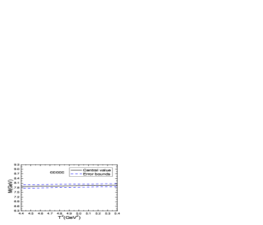
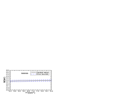
Then we take account of all uncertainties of the parameters, and obtain the values of the masses and pole residues of the fully-heavy pentaquark states,

$$M_{cccc\bar{c}} = 7.93\pm 0.15\,\rm{GeV}\,,$$

$$M_{bbbb\bar{b}} = 23.91\pm 0.15\,\rm{GeV}\,,$$

$$\lambda_{cccc\bar{c}} = (0.68\pm 0.21)\times 10^{-1}\,\rm{GeV}^{6}\,,$$

$$\lambda_{bbbb\bar{b}} = 2.43\pm 0.78\,\rm{GeV}^{6}\,,$$ (16)

which are also shown plainly in Fig.2. From Fig.2, we can see that the predicted masses are rather stable with variations of the Borel parameters, the uncertainties come from the Borel parameters are rather small, there appear very flat platforms.

Figure 2: The masses of the fully-heavy pentaquark states with variations of the Borel parameters $T^{2}$.

In the QCD sum rules, J. R. Zhang obtains the predictions of the masses $M_{cccc\bar{c}}=7.38^{+0.20}_{-0.22}\,\rm{GeV}$ and $M_{bbbb\bar{b}}=21.56^{+0.17}_{-0.15}\,\rm{GeV}$ for the $\Omega_{QQQ}\eta_{Q}$ type pentaquark molecular states with the spin-parity $J^{P}={\frac{3}{2}}^{-}$ [18]. In the modified chromo-magnetic interaction model, H. T. An et al obtain the predictions of the masses $7948.8\,\rm{MeV}$ and $7863.6\,\rm{MeV}$ for the $cccc\bar{c}$ pentaquark states with the spin-parity $J^{P}={\frac{1}{2}}^{-}$ and ${\frac{3}{2}}^{-}$, respectively, and $23820.7\,\rm{MeV}$ and $23774.8\,\rm{MeV}$ for the $bbbb\bar{b}$ pentaquark states with the spin-parity $J^{P}={\frac{1}{2}}^{-}$ and ${\frac{3}{2}}^{-}$, respectively [19]. The predictions in Ref.[18] and Ref.[19] are quite different. The present predictions $M_{cccc\bar{c}}=7.93\pm 0.15\,\rm{GeV}$ and $M_{bbbb\bar{b}}=23.91\pm 0.15\,\rm{GeV}$ for the pentaquark states with the spin-parity $J^{P}={\frac{1}{2}}^{-}$ are compatible with that of Ref.[19] within uncertainties.

The decays of the $P_{QQQQ\bar{Q}}$ pentaquark states can take place through the fall-apart mechanism,

$$P_{cccc\bar{c}} \to J/\psi\,\Omega_{ccc}\,,$$

$$P_{bbbb\bar{b}} \to \Upsilon\,\Omega_{bbb}\,,$$ (17)

according to the predicted masses from the QCD sum rules [8], we can search for the $P_{QQQQ\bar{Q}}$ pentaquark states in the $J/\psi\Omega_{ccc}$ and $\Upsilon\Omega_{bbb}$ invariant mass spectrum at the LHCb, CEPC, FCC and ILC in the future. The triply-heavy baryon states $\Omega_{ccc}$ and $\Omega_{bbb}$ have not been observed yet, and we can search for them in the decay chains, $\Omega_{ccc}\to\Omega_{ccs}\,\pi^{+}\to\Omega_{css}\,\pi^{+}\pi^{+}\to\Omega_{sss}\,\pi^{+}\pi^{+}\pi^{+}$ and $\Omega_{bbb}\to\Omega_{bbs}\,J/\psi\to\Omega_{bss}\,J/\psi J/\psi\to\Omega_{sss}\,J/\psi J/\psi J/\psi$ through the weak decays $c\to su\bar{d}$ and $b\to c\bar{c}s$ at the quark level. We should bear in mind that the baryon states $\Omega_{ccs}({\frac{1}{2}}^{+})$, $\Omega_{ccs}({\frac{3}{2}}^{+})$, $\Omega_{bbs}({\frac{1}{2}}^{+})$, $\Omega_{bbs}({\frac{3}{2}}^{+})$ and $\Omega_{bss}({\frac{3}{2}}^{+})$ have also not been observed yet, we can search for those baryon states as a byproduct.

4 Conclusion

In the present work, we construct the diquark-diquark-antiquark type five-quark currents with the same flavor to study the fully-heavy pentaquark states with the spin-parity $J^{P}={\frac{1}{2}}^{-}$ via the QCD sum rules. After tedious analytical and numerical calculations, we obtain the masses and pole residues $M_{cccc\bar{c}}=7.93\pm 0.15\,\rm{GeV}$, $M_{bbbb\bar{b}}=23.91\pm 0.15\,\rm{GeV}$, $\lambda_{cccc\bar{c}}=(0.68\pm 0.21)\times 10^{-1}\,\rm{GeV}^{6}$, $\lambda_{bbbb\bar{b}}=2.43\pm 0.78\,\rm{GeV}^{6}$. We can search for the fully-heavy pentaquark states in the $J/\psi\Omega_{ccc}$ and $\Upsilon\Omega_{bbb}$ invariant mass spectrum at the LHCb, CEPC, FCC and ILC in the future, and confront the predictions to the experimental data. And we can take the pole residues as the basic input parameters to explore the strong decays of the fully-heavy pentaquark states with the three-point QCD sum rules.

Appendix

Now we give an example to illustrate why the end-point divergences appear in Eqs.(12)-(13). At the lowest order, we often encounter the typical integral,

$$I_{11} = \int d^{4}k_{1}\frac{1}{k_{1}^{2}-m_{1}^{2}}\frac{1}{(q-k_{1})^{2}-m_{2}^{2}}\,,$$ (18)

and calculate it by using the Cutkosky’s rules,

$$I_{11} = \frac{(-2\pi i)^{2}}{2\pi i}\int_{(m_{1}+m_{2})^{2}}^{\infty}dt\frac{1}{t-q^{2}}\int d^{4}k_{1}k^{4}k_{2}\delta^{4}(k_{1}+k_{2}-q)\delta(k_{1}^{2}-m_{1}^{2})\delta(k_{2}^{2}-m_{2}^{2})$$ (19)

$$= \frac{(-2\pi i)^{2}}{2\pi i}\int_{(m_{1}+m_{2})^{2}}^{\infty}dt\frac{1}{t-q^{2}}\frac{\pi}{2}\frac{\sqrt{\lambda(t,m_{1}^{2},m_{2}^{2})}}{t}\,,$$

which is free of end-point divergence. At the second Feynman diagram in Fig.1, we often encounter the typical integral,

$$I_{22} = \int d^{4}k_{1}\frac{1}{(k_{1}^{2}-m_{1}^{2})^{2}}\frac{1}{((q-k_{1})^{2}-m_{2}^{2})^{2}}\,,$$ (20)

again we calculate it by using the Cutkosky’s rules,

$$I_{22} = \frac{\partial^{2}}{\partial A\partial B}\int d^{4}k_{1}\frac{1}{k_{1}^{2}-A}\frac{1}{(q-k_{1})^{2}-B}\mid_{A\to m_{1}^{2};B\to m_{2}^{2}}$$ (21)

$$= \frac{\partial^{2}}{\partial A\partial B}\frac{(-2\pi i)^{2}}{2\pi i}\int_{(\sqrt{A}+\sqrt{B})^{2}}^{\infty}dt\frac{1}{t-q^{2}}\int d^{4}k_{1}k^{4}k_{2}\delta^{4}(k_{1}+k_{2}-q)\delta(k_{1}^{2}-A)\delta(k_{2}^{2}-B)$$

$$= \frac{\partial^{2}}{\partial A\partial B}\frac{(-2\pi i)^{2}}{2\pi i}\int_{(\sqrt{A}+\sqrt{B})^{2}}^{\infty}dt\frac{1}{t-q^{2}}\frac{\pi}{2}\frac{\sqrt{\lambda(t,A,B)}}{t}$$

$$= \frac{(-2\pi i)^{2}}{2\pi i}\int_{(m_{1}+m_{2})^{2}}^{\infty}dt\frac{1}{t-q^{2}}\frac{\pi}{2}\frac{2(m_{1}^{2}+m_{2}^{2}-t)}{\sqrt{\lambda(t,m_{1}^{2},m_{2}^{2})}^{3}}\,.$$

In the limit $m_{1}^{2}=m_{2}^{2}=m_{Q}^{2}$, we obtain

$$\int_{(m_{1}+m_{2})^{2}}^{\infty}dt\frac{1}{t-q^{2}}\frac{1}{\sqrt{\lambda(t,m_{1}^{2},m_{2}^{2})}^{3}} = \int_{4m_{Q}^{2}}^{\infty}dt\frac{1}{t-q^{2}}\frac{1}{\sqrt{t(t-4m_{Q}^{2})}^{3}}\,,$$ (22)

divergence at the end-point $t=4m_{Q}^{2}$ appears. The end-point divergence $\frac{1}{\sqrt{s-(\sqrt{r}+m_{Q})^{2}}^{5}}$ appears at the first diagram in Fig.1, the calculations are analogous.

References

• [1] S. L. Olsen, T. Skwarnicki and D. Zieminska, Rev. Mod. Phys. 90 (2018) 015003.
• [2] N. Brambilla, S. Eidelman, C. Hanhart, A. Nefediev, C. P. Shen, C. E. Thomas, A. Vairo and C. Z. Yuan, Phys. Rept. 873 (2020) 1.
• [3] F. K. Guo, C. Hanhart, U. G. Meissner, Q. Wang, Q. Zhao and B. S. Zou, Rev. Mod. Phys. 90 (2018) 015004.
• [4] R. Aaij et al, Phys. Rev. Lett. 119 (2017) 112001.
• [5] R. Aaij et al, Sci. Bull. 65 (2020) 1983.
• [6] R. F. Lebed, R. E. Mitchell and E. S. Swanson, Prog. Part. Nucl. Phys. 93 (2017) 143.
• [7] A. Esposito, A. Pilloni and A. D. Polosa, Phys. Rept. 668 (2017) 1.
• [8] Z. G. Wang, AAPPS Bull. 31 (2021) 5.
• [9] Z. G. Wang and Z. H. Yan, Eur. Phys. J. C78 (2018) 19.
• [10] Z. G. Wang, Eur. Phys. J. C78 (2018) 826.
• [11] Z. G. Wang, Acta Phys. Polon. B49 (2018) 1781.
• [12] R. Aaij et al, Phys. Rev. Lett. 115 (2015) 072001.
• [13] R. Aaij et al, Phys. Rev. Lett. 122 (2019) 222001.
• [14] R. Aaij et al, Sci. Bull. 66 (2021) 1278.
• [15] H. X. Chen, W. Chen, X. Liu and S. L. Zhu, Phys. Rept. 639 (2016) 1.
• [16] A. Ali, J. S. Lange and S. Stone, Prog. Part. Nucl. Phys. 97 (2017) 123.
• [17] Y. R. Liu, H. X. Chen, W. Chen, X. Liu and S. L. Zhu, Prog. Part. Nucl. Phys. 107 (2019) 237.
• [18] J. R. Zhang, Phys. Rev. D103 (2021) 074016.
• [19] H. T. An, K. Chen, Z. W. Liu and X.Liu, Phys. Rev. D 103 (2021) 074006.
• [20] R. M. Albuquerque, J. M. Dias, K. P. Khemchandani, A. M. Torres, F. S. Navarra, M. Nielsen and C. M. Zanetti, J. Phys. G46 (2019) 093002.
• [21] Z. G. Wang and Z. Y. Di, Eur. Phys. J. C79 (2019) 72.
• [22] Z. G. Wang, Acta Phys. Polon. B51 (2020) 435.
• [23] Z. G. Wang, Eur. Phys. J. C79 (2019) 184.
• [24] Z. G. Wang, Eur. Phys. J. C77 (2017) 432.
• [25] Z. G. Wang and Z. Y. Di, Acta Phys. Polon. B50 (2019) 1335.
• [26] Z. G. Wang, Eur. Phys. J. C79 (2019) 489.
• [27] Z. G. Wang, Phys. Rev. D102 (2020) 014018.
• [28] Z. G. Wang, Int. J. Mod. Phys. A35 (2020) 2050003.
• [29] Z. G. Wang, Int. J. Mod. Phys. A36 (2021) 2150071.
• [30] M. A. Shifman, A. I. Vainshtein and V. I. Zakharov, Nucl. Phys. B147 (1979) 385, 448.
• [31] L. J. Reinders, H. Rubinstein and S. Yazaki, Phys. Rept. 127 (1985) 1.
• [32] P. Colangelo and A. Khodjamirian, hep-ph/0010175.
• [33] P. A. Zyla et al, Prog. Theor. Exp. Phys. 2020 (2020) 083C01.
• [34] Z. G. Wang, Commun. Theor. Phys. 73 (2021) 065201.