Multi-Cycle-Consistent Adversarial Networks for Edge Denoising of Computed Tomography Images

Abstract.

As one of the most commonly ordered imaging tests, computed tomography (CT) scan comes with inevitable radiation exposure that increases the cancer risk to patients. However, CT image quality is directly related to radiation dose, thus it is desirable to obtain high quality CT images with as little dose as possible. CT image denoising tries to obtain high dose like high-quality CT images (domain $Y$) from low dose low-quality CT images (domain $X$), which can be treated as an image-to-image translation task where the goal is to learn the transform between a source domain $X$ (noisy images) and a target domain $Y$ (clean images). Recently, cycle-consistent adversarial denoising network (CCADN) has achieved state-of-the-art results by enforcing cycle-consistent loss without the need of paired training data, since the paired data is hard to collect due to patients’ interests and the cardiac motion. On the other hand, out of concerns on patients’ privacy and data security, protocols typically require clinics to perform medical image processing tasks including CT image denoising locally, i.e., edge denoising. Therefore, the network models needs to achieve high performance under various computation resource constraints including memory and performance. Our detailed analysis of CCADN raises a number of interesting questions which point to potential ways to further improve its performance using same or even less computation resources. For example, if the noise is large leading to significant difference between domain $X$ and domain $Y$, can we bridge $X$ and $Y$ with a intermediate domain $Z$ such that both the denoising process between $X$ and $Z$ and that between $Z$ and $Y$ are easier to learn? As such intermediate domains lead to multiple cycles, how do we best enforce cycle-consistency? Driven by these questions, we propose a multi-cycle-consistent adversarial network (MCCAN) that builds intermediate domains and enforces both local and global cycle-consistency for edge denoising of CT images. The global cycle-consistency couples all generators together to model the whole denoising process, while the local cycle-consistency imposes effective supervision on the process between adjacent domains. Experiments show that both local and global cycle-consistency are important for the success of MCCAN, which outperforms CCADN in terms of denoising quality with slightly less computation resource consumption.

1. Introduction

The privacy and security of patient data have always been the primary concern in medical applications among hospitals and clinics. As such, protocols typically require medical image processing tasks such as denoising (Shan et al., 2018; Wolterink et al., 2017; Chen et al., 2017; Yang et al., 2018), segmentation (Xu et al., 2019; Wang et al., 2020; Liu et al., 2019; Xu et al., 2018b; Zhang et al., 2018, 2020, 2021), and diagnosis (Xu et al., 2020) to be performed locally, i.e., on the edge. However, local machines and devices are usually with rather limited computation resources including memory capacity and performance compared with those in the cloud. The constrained resources can have profound impact on the design of medical image processing algorithms. In this paper, we will use Computed tomography (CT) image denoising as a vehicle to demonstrate it.

CT is one of the most widely used medical imaging modality for showing anatomical structures (You et al., 2018). The foremost concern of CT examination is the associated exposure to radiation, which is known to increase the lifetime risk for death of cancer (Hobbs et al., 2018). The radiation dose can be lowered at the cost of increased noise (Li et al., 2014; You et al., 2018). Such noise in CT image leads to both degraded perceptual quality and degraded diagnostic confidence of a doctor. A general principle in dose management in practice is “as low as reasonably achievable” (Mayo-Smith et al., 2014). Thus the resulted images are denoised for minimized the loss on perceptual quality and diagnostic confidence of radiologists. Even with tremendous effort and significant progresses in the past few decades, the radiation exposure of CT scan was still estimated to account for up to two percent of cancer in United States (Sodickson et al., 2009).

Various deep neural network (DNN) based methods exist for CT image denoising (Shan et al., 2018; Wolterink et al., 2017; Chen et al., 2017; Yang et al., 2018), which require paired clean and noisy images for training. Yet paired images are hard to collect due to patients’ interests and the cardiac motion. Therefore, simulations are usually used to generate such paired data, where the simulated noise patterns can be different from the real ones, leading to biased training results (Kang et al., 2018). To address this issue, recently cycle-consistent adversarial denoising network (CCADN) was proposed in (Kang et al., 2018), which formulates CT image denoising as an image-to-image translation problem without paired training data. CCADN consists of two generators: One transforms noisy CT images (domain $X$) to clean ones (domain $Y$) and the other transforms clean CT images (domain $Y$) to noisy ones (domain $X$). Both generators are trained by adversarial loss. In addition, they form a cycle where a noisy CT image can be transformed to a clean one and transformed back to a noisy one (i.e., $X\rightarrow Y\rightarrow X$). Cycle-consistency loss is defined by the difference between the two noisy CT images, which is a key component to control the training of both generators for better performance. Cycle-consistency loss is also imposed for $Y\rightarrow X\rightarrow Y$ transform. However, CCADN only works well when the noise levels are low. This is due to the fact that it only contains two domains $X$ and $Y$ and therefore its efficacy degrades as the noise becomes stronger, leading to larger differences between $X$ and $Y$ that are harder to learn. A larger neural network with stronger representation power is needed, which may not be feasible with the limited computation resources on the edge.

To enhance the performance of CCADN without increasing the resource consumption, as shown in Fig. 1, we propose to establish an intermediate domain between the original noisy image domain $X$ and clean image domain $Y$, and decompose the denoising task into multiple coupled steps such that each step is easier to learn by DNN-based models. Specifically, we construct an additional domain $Z$ with images of intermediate noise level between $X$ and $Y$. These images can be considered as a step stone in the denoising process and provide additional information for the training of the denoising network. The multi-step framework particularly suits the denoising problem: while it is difficult to either find or define a good collection of images in the “half-cat, half dog” domain in “cat-to-dog” type of image translation problems, a domain $Z$ of images with intermediate level of noise exist naturally. In addition, when the denoising problem (two domains) is divided into several subproblems ($N$ domains), each subproblem is much easier to solve. In this way, the network complexity for each subproblem (e.g., number of parameters) is usually lower than $1/(N-1)$ of the original network (Xu et al., 2018a). Thus, the overall computation consumption can be reduced.

Figure 1. Comparison of domians in (a) CCADN and (b) the proposed MCCAN. CCADN performs single-cycle-consistent adversarial training with two domains, while the proposed MCCAN performs multiple-cycle-consistent adversarial training with more than two domains, e.g., three.

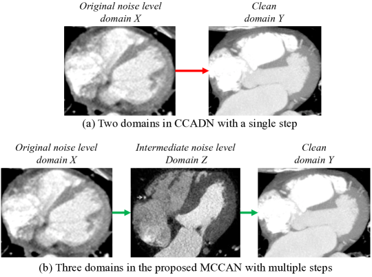
With the new domain $Z$, we further propose a multi-cycle-consistent adversarial network to perform the multi-step denoising, which builds multiple cycles of different scales (global cycles and local cycles) between the domains while enforcing the corresponding cycle-consistencies. Specifically, global cycles combine all the generators and domains together to model the entire denoising process. The local cycles serve two purposes. First, they impose effective supervision on the generators between adjacent domains. Second, while each step is easier, the multi-step framework leads to deeper networks and makes it challenging for end-to-end training. The local cycles can provide gradient from the supervised training of easier tasks on shallower networks and thus alleviating the problem. The experimental results show that both global cycles and local cycles are necessary, and our method MCCAN outperforms the state-of-the-art competitor CCADN with a slightly less resource consumption.

2. Related Works

2.1. CT Image Denoising

Numerous CT image denoising methods can be categorized as three types: signogram filtering-based method, iterative reconstruction, and image space denoising (You et al., 2018). The first two types of methods are usually embedded within the CT scanner as commercial algorithms, thus we focus more on the last type of methods for research.

Signogram filtering-based method perform in the original projection space before filtered backprojection is applied to reconstruct images (Manduca et al., 2009; Liu et al., 2017). One common advantage of these method is the noise properties in projection space are fairly well-understood. However, the image sharpness may degrade because the edges are not well-defined in projection data (Li et al., 2014).

Iterative reconstruction are considered the most accurate one by using statistical assumptions about the noise properties in projection space, prior information in image space, and various accurate information of the specific scanner (Nuyts et al., 1998). However, the implementation highly depend on specific scanner models and is very computational extensive for each scan (Xu and Mueller, 2007; Li et al., 2014).

Image space denoising is performed on the reconstructed images and thus the computation cost is much lower than that in the first two category. In recently years, deep neural networks and various method developed in other area are combined with CT image denoising including GAN, autoencoder, perceptual loss, transfer learning, 3D convolution (Shan et al., 2018; Wolterink et al., 2017; Chen et al., 2017; Yang et al., 2018). Mostly recently, CycleGAN is applied to CT denoising as CCADN and achieves better results than state-of-the-art (Kang et al., 2018).

It can be hard to find a standard metric to measure the denoising performance when there is no paired samples for test. For the protection of patients and operators, repetitive CT scan is usually not permitted due to the additional radiation dose. Even if repetitive scan is available, the cardiac motion or the changed operating condition will make two scans different. This problem is alleviated by simulating corresponding low dose images from high dose images with noise modeling (Karmazyn et al., 2009; Green et al., 2018). However, noise should be added in the sinogram domain in the synthetic CT scan images, which is too difficult to implement without the assistance from the CT scanners’ vendor (Kang et al., 2018). Besides, the additional noise pattern can be different from the real noise pattern. This will introduce bias in the data and end up with biased denoising models.

2.2. Image-to-Image Translation

Our work are closely related to some of the popular image-to-image translation models using generative adversarial networks (Isola et al., 2017) or neural style transfer (Johnson et al., 2016). Image-to-image translation also includes some other artifact removal problems similar to denoising such as raindrop removal and shadow removal (Qian et al., 2018; Liu et al., 2018; Wang et al., 2018). (Wang et al., 2018) uses a joint-learned two-step approach for shadow removal where one conditional GAN (Mirza and Osindero, 2014) is used to detect the shadow region and the result is used by another conditional GAN for shadow removal. However these two steps are mostly specific to a small set of problems and can not be applied to other cases with more steps.

While the using of cycle consistency loss has achieved significant progresses (Zhu et al., 2017; Yi et al., 2017; Kim et al., 2017), these models still have some drawbacks. CycleGAN often succeeds on translation of low level features including color and texture but has little success on tasks with geometric changes (Zhu et al., 2017). We anticipate that the multiple-step approach can potentially alleviate this problem. On the other hand, CycleGAN can be inefficient for translation in multiple domains, because the number of translation model grows quadratically with the number of domains. Motivated by this, StartGAN and ComboGAN (Choi et al., 2017; Anoosheh et al., 2018) propose new models to get better scalability. The training method of CycleGAN in the facial attribute transfer experiment in (Choi et al., 2017) is essentially the MCCAN without global cycles. The ComboGAN is used to perform multi-step transformation (e.g. changing gender after changing hair color). The results show that the image quality degrade with more translation steps. We analyze the possible reasons, the lack of global cycles, in Section 3.

Coupled GAN (CoGAN) is proposed in (Liu and Tuzel, 2016) to learn a joint distribution in different domains without paired samples. Based on the assumption that deep neural networks learn a hierarchical feature representation, CoGAN enforces the GANs to decode high-level semantics in the same way by sharing the weights. In order to translate a image $x$ in domain $X$ to domain $Y$, it have to find the random vector that generates $x$ through the generator for $X$ and they apply the generator for $Y$ to this random vector. Such a search process could be very time consuming (Gatys et al., 2016). Another limitation is the transformation only success when $x$ is covered by the generator for $X$ (can be generated by this generator). While it is not discussed in their paper, we found that their approach implicitly uses a feature map domain as a bridge for the translation. Specifically, if we assume the query image is always covered by the corresponding generator, their structure can be consider as building a domain graph what each images domain is connected to a central feature map domain. When doing the translation, it always translate as $X\to Z\to Y$ where $Z$ is the feature map domain. In this paper, we equip MCCAN with available CT images from different domains (radiation dose) directly for the denoising task while without increasing the resource consumption.

3. Multi-Cycle-Consistent Adversarial Networks

Given training images that are either labelled as noisy (domain $X$) or clean (domain $Y$), we first construct a new domain $Z$ which contains images with an intermediate noise level between $X$ and $Y$. How to obtain $Z$ is flexible in practice. It can either be obtained from $X$ and $Y$ by separating out those images with intermediate noise level if available, or from images scanned with medium dose, or from common techniques including injecting intermediate level of noise to the images in $Y$.

(a)

(b)

Figure 2. (a) Structure of MCCAN and (b) its cycles. The arrows inside each domain denote the computation of cycle-consistency loss. The solid and dashed arrows across domains form global and local cycles, respectively. For clarity, we only show cycles from left to right. Symmetric cycles going from right to left also exist but are not shown.

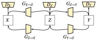
With CT images from three domains, the multi-step denoising architecture of MCCAN is shown in Fig. 2a. We train four convolutional neural networks as generators and three as discriminators. Arrows in Fig. 2a define how images are transformed in the training stage. Specifically, the generator $G_{X\to Z}$ aims to transform an image from $X$ to $Z$. $G_{Z\to X}$, $G_{Z\to Y}$, and $G_{Y\to Z}$ can be interpreted similarly. Discriminators $D_{X}$, $D_{Y}$, and $D_{Z}$ aim to distinguish the “real” images originally belonging to the domains $X$, $Y$, and $Z$ respectively from the “fake” images transformed from other domains.

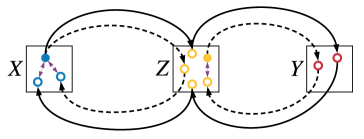
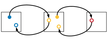
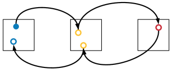
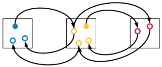
As the MCCAN structure in Fig. 2a contains thee domains, there are multiple ways in which we can construct cycles (paths where an image from a source domain is transformed through one (in (Zhu et al., 2017)) or several other domains (in this paper) and back to the source domain) for cycle-consistent loss. In particular, we introduce two types of cycles as shown in Fig. 2b. In this figure, each dot represents an image, which is color-coded based on the domain. The solid ones represent the images originally in the domain (“real” ones), and the hollow ones represent those transformed from another domain (“fake” ones). As such, the dashed arrows form the local cycles, each of which goes across only two adjacent domains. On the other hand, the solid arrows constitute a global cycle that starts from $X$ through $Z$, $Y$, $Z$, and back to $X$ sequentially. Note that in the figure we only show half of the cycles (from left to right) for clarity, and the other half which are from right to left and symmetric to the ones shown also exist. We then enforce cycle-consistency loss, which measures the difference between the original images and the final images produced at the end of the cycle as represented by the small arrows within each domain in Fig 2b. Ideally, the images transformed back to the source domain should be identical to the original images. The cycle-consistency loss is applied to every cycle, no matter whether it is local or a global.

The global cycles are important for the denoising performance due to the following reason. In the inference stage, an input noisy CT image $x$ in domain $X$ will be transformed by $G_{X\to Z}$ and $G_{Z\to Y}$ sequentially, which means $G_{X\to Z}$ and $G_{Z\to Y}$ are coupled by data dependency. Without global cycles, $G_{X\to Z}$ and $G_{Z\to Y}$ will be trained independently. The global cycles enable the joint training of the generators, which models the denoising path used in the inference stage for better consistency.

The local cycles are also important to address two issues in the training. First, the global cycles go through all the four generators and have long paths for the gradient to back-propagate, which makes the end-to-end optimization difficult. The locals cycles are shallow and have shorter paths for the gradient to back-propagate. Second, adversarial training only enforces the generators to output “fake” images identically distributed as the original “real” images in the intermediate domain $Z$. However, they do not necessarily preserve the meaningful content in the inputs, which is critical for the denoising task. The local cycle-consistency supervises each generator to learn to transform images while preserving their meaningful content from the inputs more easily.

(a)

(b)

(c)

(d)

Figure 3. Comparison of (a) CCADN, (b) MCCAN without global cycles (c) MCCAN without local cycles, and (d) MCCAN. For the clarity of presentation, we only show cycles from left to right and symmetric cycles from right to left also exist.

In summary, our MCCAN has three major advantages over CCADN. First, it decomposes the one-step transform into multiple steps using constructed images in a intermediate domain as a step stone. Second, it not only incorporates global cycles that model the denoising path in the inference stage for consistency, but also uses local cycles that provide strong supervision to facilitate the more challenging training process. Third, the network structure of generators can be simplified due to the relatively easier task in each transformation, thus potentially reducing memory and computation consumption.

Note that in the discussion so far, only one intermediate domain was assumed. It is also possible to include more than one intermediate domains with more global and local cycles. However, our study suggests that any additional domains beyond one will not introduce further performance gain in the dataset we explored.

3.1. Network Architectures

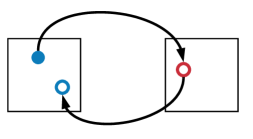
We compare MCCAN with a state-of-the-art CT denoising framework CCADN (Kang et al., 2018). In order to see how the local cycles and global cycles contribute to the final performance, we also implement and compare MCCAN without local cycles and without global cycles respectively as ablation study. The various structures are shown in Fig. 3. or the clarity of presentation, only cycles from left to right are shown, but symmetric cycles from right to left also exist.

(a)

(b)

Figure 4. Network architectures of generators for (a) MCCAN, and (b) CCADN. ResBlock represents residual blocks (He et al., 2016). For MCCAN, MCCAN without local cycles, and MCCAN without global cycles, the network architecture in (b) are shared. Because every generator in such frameworks, the generator only transfer between adjacent domains. Nevertheless, generators in CCADN need to transfer images between more than one domains, thus with larger networks.

To ensure that model sizes, computation operations, and number of training epochs are the same for fair comparisons, different network structures are applied in experiments. Generally speaking, all discriminators are used for a same discrimination task in each image domain, so all discriminators share a same network structure. However, generator structures are different for different tasks, since the capability of generators denoising by one step and the capability of generators denoising by more steps, two step here, are supposed to be different.

Traditional convolution networks are used as the discriminator for all domains in all experiments. In terms of the generators, since there are two types of generators in our experiments, different network architectures are utilized in our experiments. Both network architectures share the same layers for pre-processing and post-processing, as shown in Fig. 4. However, the generators transferring images images between two domains that are more different from each other should have more layers and parameter, and vice versa. So the generators in CCADN is implemented with more residual blocks (ResBlock) as shown in Fig. 4b, while generators in MCCAN, MCCAN without local cycles, and MCCAN without global cycles are all implemented as the network architecture shown in Fig. 4a. As a result, the total number of parameters used in each experiment in inference is around 11M to make sure that each method consumes the same memory resources.

3.2. Training Objectives

Finally, we state the training objective used in our framework. Denote $\{G\}$ and $\{D\}$ as the set of generators and discriminators respectively. Denote $I\in\{X,Y,Z\}$ as one domain and $D_{I}$ as the discriminator associated with domain $I$. We let $C_{i}$ be a cycle and $P_{i,j}$ be a path of half $C_{i}$ that has the same source domain, where $i,j$ are used to distinguish different cycles and paths merely. For example, $X\rightarrow Z\rightarrow X$ is a cycle, saying $C_{1}$, thus we can have $P_{1,1}=X\rightarrow Z$, and $P_{1,2}=Z\rightarrow X$, which are both half cycles of $C_{1}$. $\{P_{I}\}$ represents the set of all the paths that end at domain $I$. We denote $I_{C_{i}}$ as the source domain of $C_{i}$ and $G_{P_{i,j}}$ as the ordered function composition of the generators in $P_{i,j}$. Thus, the total adversarial loss is

(1) $$\mathcal{L}_{GAN}(\{G\},\{D\})=\sum_{I\in\{X,Y,Z\}}\sum_{P_{i,j}\in\{P_{I}\}}\mathcal{L}_{GAN}(I,P_{i,j})$$

where $\mathcal{L}_{GAN}(I,P_{i,j})$ is the adversarial loss associated with domain $I$ and the transform path $P_{i,j}$. $\mathcal{L}_{GAN}(I,P_{i,j})$ is obtained by

(2) $$\mathcal{L}_{GAN}(I,P_{i,j})= \mathbb{E}_{y\sim p_{data}(I)}[\log{D_{I}(y)}]$$

$$+\mathbb{E}_{x\sim p_{data}(I_{C_{i}})}[log(1-D_{I}(G_{P_{i,j}}(x)))]$$

where $p_{data}$ is the distribution of “real” images in a domain and $D_{I}(x)$ represents the probability determined by $D_{I}$ that $x$ is a “real” image from domain $I$ rather than a “fake” one transformed by generators from another domain.

The cycle-consistency loss is associated with each $C_{i}$, defined as

(3) $$\mathcal{L}_{\text{cyc}}(\{G\},C_{i})=\mathbb{E}_{x\sim p_{\text{data}}(I_{C_{i}})}[|G_{C_{i}}(x)-x|_{1}].$$

The identity loss is associated with each generator in ${G}$, defined as

(4) $$\mathcal{L}_{\text{idt}}(\{G\})= \sum_{I\in\{X,Y,Z\}}\sum_{J\in\{X,Y,Z\},J\neq I}($$

$$\mathbb{E}_{x\sim p_{\text{data}}(I)}[|G_{J\rightarrow I}(x)-x|_{1}]).$$

The final optimization problem we solve in the training stage is:

(5) $$\{G\}^{*}= \arg\min_{\{G\}}\max_{\{D\}}(\mathcal{L}_{GAN}(\{G\},\{D\})$$

$$+\lambda_{\text{cyc}}\sum_{C_{i}\in\{C\}}\mathcal{L}_{cyc}(\{G\},C_{i})$$

$$+\lambda_{\text{idt}}\cdot\mathcal{L}_{\text{idt}}(\{G\}).$$

where $\lambda_{\text{cyc}}$ and $\lambda_{\text{idt}}$ are set to 10 and 0.5 respectively in our experiments.

4. Experiments and Results

4.1. Experiments Setup

The original dataset contains 200 clean (normal-dose) 3D cardiac CT images and 200 noisy (low-dose) ones from various patients for training, and separate 11 images for test. The dataset is captured from 6 patients (3 for normal dose and 3 for low dose). All examinations are performed with a wide detector 256-slice MDCT scanner (Brilliance iCT; Philips Healthcare) providing 8cm of coverage. Each 2D CT image is of size 512$\times$512, which is then randomly cropped into 256$\times$256 for data augmentation. We extract the noise pattern from the noisy CT images and add them to the clean CT images with a weighting factor $\frac{1}{2}$ to generate new CT images with the intermediate noise level.

Following existing works (Arapakis et al., 2014; Wolterink et al., 2017; Yang et al., 2018), we use the mean and standard deviation (SD) of pixels in homogeneous regions of interest chosen by our radiologists to quantitatively judge the quality of CT images. The mean, which reflects substance information, should be as close to that in the origin image as possible, and the standard deviation, which reflects noise, should be as low as possible.

(a) Original noisy CT images

(b) Images denoised by CCADN

(c) Images denoised by MCCAN without local cycles

(d) Images denoised by MCCAN without global cycles

(e) Images denoised by MCCAN

Figure 5. (a) Original noisy CT images and the corresponding ones denoised by (b) CCADN(Kang et al., 2018), (c) MCCAN without local cycles, (d) MCCAN without global cycles, and (e) MCCAN. (Best viewed in color.)

(a) Original noisy CT images

(b) Images denoised by CCADN

(c) Images denoised by MCCAN without local cycles

(d) Images denoised by MCCAN without global cycles

(e) Images denoised by MCCAN

Figure 6. (a) Original noisy CT images and the corresponding ones denoised by (b) CCADN(Kang et al., 2018), (c) MCCAN without local cycles, (d) MCCAN without global cycles, and (e) MCCAN. (Best viewed in color.)

Figure 7. An image transformed through X$\rightarrow$Z$\rightarrow$Y$\rightarrow$Z$\rightarrow$X cycle in Fig. 3. The noise level decreases along X$\rightarrow$Z$\rightarrow$Y and increases along Y$\rightarrow$Z$\rightarrow$X, which conforms to our design.

Table 1. Comparison of denosing performance between configurations using different number of domains in MCCAN over the selected areas in Fig. 5a.

Method	Mean	SD
Original	1321.2	84.5
CCADN (two domains)(Zhu et al., 2017)	1284.1	67.8
MCCAN (three domains)	1251.4	60.6
MCCAN (four domains)	1244.1	77.6

We first discuss how the number domains affects the denoising performance of MCCAN. Then we compare MCCAN with a state-of-the-art CT denoising framework CCADN (Kang et al., 2018), which is also based on cycle-consistency loss but contains only two domains. In order to see how the local cycles and global cycles contribute to the final performance, we also implement and compare MCCAN without local cycles and without global cycles respectively as ablation study. The various structures are shown in Fig. 3. We train all the networks following the setting in (Zhu et al., 2017). As shown in Fig. 5 and Fig. 6, six images chosen by our radiologist are used for the qualitative evaluation, and 12 homogeneous areas annotated by red rectangles and numbered are used for quantitative evaluation. All network sizes and number of training epochs are the same for fair comparisons.

4.2. Discussion of Number of Domains

As shown in Table 1, the average mean and SD in five areas indicated in Fig. 5a are presented. Compared with the original image, CCADN can largely reduce the noises by about 20%. MCCAN with three domains can further improve the image quality with reduced noise by about 8.4%. However, MCCAN with four domains obtains reduced improvement compared with that with three domains and CCADN. Actually this is expected. More domains require more datasets with different levels of noise, and the difference between the datasets with adjacent levels of noise is smaller. When the difference gets too small, the network can no longer learn it effectively, resulting in degraded performance. For our collected dataset, the optimal number of domains is three, and other datasets may have a different optimal number of domains. How to effectively identify the optimal number of domains for a given dataset can be an interesting problem worth further studying.

4.3. Comparison with the State-of-the-art Method

Table 2. Comparison of number of parameters (memory) and operations (computation) between the proposed method and the state-of-the-art CCADN for inference. Note that there is one generator in CCADN, while there are two in MCCAN. FLOP stands for floating point operation.

Method	Number of parameters	FLOPs
CCADN(Zhu et al., 2017)	11.4M	745G
MCCAN w/o local cycles	11.0M	668G
MCCAN w/o global cycles	11.0M	668G
MCCAN	11.0M	668G

Table 3. Mean and SD of the selected areas in Fig. 5.

Method	Original		CCADN (Zhu et al., 2017)		MCCAN w/o local cycles		MCCAN w/o global cycles		MCCAN
	Mean	SD	Mean	SD	Mean	SD	Mean	SD	Mean	SD
Area #1	1942.3	118.0	1801.2	100.2	30.9	45.2	1747.7	92.6	1712.8	89.8
Area #2	903.3	60.0	928.8	47.1	215.0	60.9	932.1	46.0	940.5	40.8
Area #3	913.6	58.1	938.2	46.0	96.7	41.2	943.5	46.4	938.0	41.3
Area #4	1944.0	132.6	1821.5	103.8	43.8	55.6	1762.2	97.3	1723.5	94.5
Area #5	903.2	53.8	930.7	42.0	255.0	70.7	934.0	43.4	942.2	36.6

Table 4. Mean and SD of the selected areas in Fig. 6.

Method	Original		CCADN (Zhu et al., 2017)		MCCAN w/o local cycles		MCCAN w/o global cycles		MCCAN
	Mean	SD	Mean	SD	Mean	SD	Mean	SD	Mean	SD
Area #1	1067.2	24.8	1057.75	20.4	87.2	12.1	1058.5	20.58	1061.9	19.53
Area #2	1568.4	62.4	1498.4	60.6	47.9	22.6	1504.0	59.1	1547.9	54.8
Area #3	1052.9	34.4	1044.1	27.9	56.4	12.3	1044.8	28.0	1047.0	24.2
Area #4	906.6	43.2	942.6	37.7	120.1	25.7	930.7	33.4	897.1	30.9
Area #5	1082.2	66.11	1191.3	51.8	254.3	43.0	1165.5	50.7	1147.3	48.8
Area #6	1233.0	76.9	1398.2	65.4	176.0	56.3	1364.6	64.4	1367.7	63.6
Area #7	992.5	230.4	968.9	190.0	340.2	67.2	1010.3	188.8	995.8	178.3

4.3.1. Comparison of Resource Consumption

The comparison of number of parameters and floating point operations (FLOPs) between the proposed method and the state-of-the-art CCADN in inference is shown in Table 2. We can notice that the number of parameters and operations of MMCAN is lightly less than that of CCADN, and MCCANs with different configurations have the same number of parameters and operations. This is because there are two generators with the same network structure in inference for MCCANs with different configurations. Note that, although MCCAN without global cycles is supposed to have the same network architecture as MCCAN, there is one extra discriminator associated with the intermediate domain $Z$. The reason for the extra discriminator is that if there is only one discriminator associated with domain $Z$, the information from both domain $X$ and domain $Y$ will help it to learn, which results in a stronger discriminator than a discriminator with only one local cycle. That is, information from global scope, both domain $X$ and domain $Y$ here, converges at the discriminator. Then the information would be propagated to generators connected with the discriminator as well as whole networks. This is what we would not want to see. Thus, two discriminators are utilized, and one for each local cycle to break the global information communication.

4.3.2. Qualitative Evaluation

We choose six representative low-dose CT images in the test dataset as shown in Fig. 5 and Fig. 6 for qualitative evaluation. The corresponding denoised images by CCADN, MCCAN without local cycles, MCCAN without global cycles, and MCCAN are shown in Fig. 5b-5e and 6b-6e respectively. From the figures we can see that CCADN can successfully reduce noise in the original images. MCCAN without local cycles completely fails to produce reasonable results. A close examination of the images reveal that interestingly the background and the substances are approximately swapped compared with the original images. This is because the high-level features of content distribution are still kept even with such swap, and the discriminator cannot identify the generated image as “fake” because of the structure diversity in the training dataset. This aligns with our discussion on the importance of local cycles in Section 2. We can take a more closer comparison on the area indicated by yellow arrows in Fig. 5 and Fig. 6. We can observe that compared with the original images and CCADN, only MCCAN can successfully remove the tiny spot indicated by a yellow arrow in Fig. 5. In addition, MCCAN and MCCAN without global cycles can remove the small hole in Fig. 6 which should not exist in the vessel. On the other hand, MCCAN without global cycles can successfully denoise the image and achieves similar quality compared with CCADN. This is expected as MCCAN without global cycles is essentially formed by two cascaded CCADNs. Finally, though MCCAN without local or cycles and the complete MCCAN have competitive visual performance with each other, the complete MCCAN has a relatively smaller noise (less spots, and more smooth boundary) visually.

To further illustrate the efficacy of the MCCAN structure, Fig. 7 shows how an image is transformed along a global cycle (the path X$\rightarrow$Z$\rightarrow$Y$\rightarrow$Z$\rightarrow$X). From the figure we can see that $X\rightarrow Z\rightarrow Y$ is an effective two-step denoising process while $Y\rightarrow Z\rightarrow X$ incrementally adds noise back.

4.3.3. Quantitative Evaluation

The quantitative results are shown in Table 3 and Table 4. CCADN can reduce the standard deviation in the 12 areas by 15%, 21%, 21%, 22%, 22%, 18%, 3%, 19%, 13%, 22%, 15%, and 18%, respectively, with resulting mean values close to those of the original images. Although MCCAN without local cycles achieves smallest standard deviation in Areas 1, 3 and 4, it leads to large mean deviation from the original images, which corresponds to the structure loss in Fig. 5c. MCCAN without global cycles has similar performance compared with CCADN, with mean values close to original and standard deviation reduction by 22%, 23%, 20%, 27%, 19%, 17%, 5%, 19%, 23%, 23%, 16%, and 18%, respectively. Finally, the complete MCCAN behaves the best among all the methods. With mean values close to original, the standard deviations are decreased by 24%, 32%, 29%, 29%, 32%, 21%, 12%, 30%, 28%, 26%, 17%, and 23%, from the original CT images, respectively.

5. Conclusions

In this paper, we propose multi-cycle-consistent adversarial network (MCCAN) for edge denoising of CT images. MCCAN builds intermediate domains and enforces both local and global cycle-consistency. The global cycle-consistency couples all generators together to model the whole denoising process, while the local cycle-consistency imposes effective supervision on the denoising process between adjacent domains. Experiments show that both local and global cycle-consistency are important for the success of MCCAN, and it outperforms the state-of-the-art competitor with slightly less resource consumption. Our code is publicly available. Considering the practical usage, the computation complexity and the denoising performance still need further improvement, and our future work will focus on optimize the denoising performance while reducing the computation operations at the same time. In the future work, we will try to apply MCCAN to other medical images such as magnetic resonance imaging (MRI) and ultra sound images, and explore the cycle design theoretically.