DecentLaM: Decentralized Momentum SGD for Large-batch Deep Training

Abstract

The scale of deep learning nowadays calls for efficient distributed training algorithms. Decentralized momentum SGD (DmSGD), in which each node averages only with its neighbors, is more communication efficient than vanilla Parallel momentum SGD that incurs global average across all computing nodes. On the other hand, the large-batch training has been demonstrated critical to achieve runtime speedup. This motivates us to investigate how DmSGD performs in the large-batch scenario.

In this work, we find the momentum term can amplify the inconsistency bias in DmSGD. Such bias becomes more evident as batch-size grows large and hence results in severe performance degradation. We next propose DecentLaM, a novel decentralized large-batch momentum SGD to remove the momentum-incurred bias. The convergence rate for both non-convex and strongly-convex scenarios is established. Our theoretical results justify the superiority of DecentLaM to DmSGD especially in the large-batch scenario. Experimental results on a variety of computer vision tasks and models demonstrate that DecentLaM promises both efficient and high-quality training.

1 Introduction

Efficient distributed training across multiple computing nodes is critical for large-scale deep learning tasks nowadays. As a principal training algorithm, Parallel SGD computes a globally averaged gradient either using the Parameter Server (PS) [22] or the All-Reduce communication primitive [37]. Such global synchronization across all nodes either incurs significant bandwidth cost or high latency that can severely hamper the training scalability.

Decentralized SGD [35, 6, 24, 25, 3] based on partial averaging has become one of the major approaches in the past decade to reduce communication overhead in distributed optimization. Partial averaging, as opposed to global averaging used in Parallel SGD, requires every node to compute the average of the nodes in its neighborhood, see Fig. 1. If a sparse topology such as one-peer exponential graph [3] is utilized to connect all nodes, each node only communicates with one neighbor each iteration and hence saves remarkable communications. Decentralized SGD can typically achieve $1.3\sim 2\times$ training time speedup without performance degradation [24, 3, 21].

Existing Decentralized SGD methods [24, 25, 46, 26, 3] and their momentum accelerated variants [55, 43, 13, 4] primarily utilize small-batch in their algorithm design. However, recent hardware advances make it feasible to store large batches in memory and compute their gradients timely. Furthermore, the total batch size naturally grows when more computing nodes participate into training. These two primary reasons lead to the recent exploration of large-batch deep training algorithms.

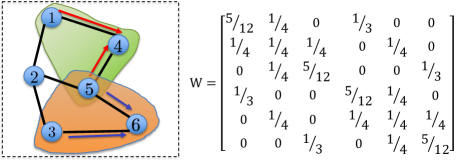
Figure 1: Illustration of decentralized methods. Nodes receive information from neighbors; they do not relay information. For example, nodes $4$ and $6$ collect information from their neighbors $\{1,5\}$ and $\{3,5\}$, respectively. Other nodes do the same but not depicted. Topology connectivity can be represented in a matrix, as shown in the right figure, see more details in Sec. 3.

In fact, large-batch training has been extensively studied in Parallel SGD. Pioneering works [15, 51, 53] find large-batch can significantly speed up Parallel SGD. First, the computation of a large-batch gradient can fully utilize the computational resources (e.g., the computing nodes, the CUDA cores and GPU memories within each node). Second, large-batch gradient will result in a reduced variance and hence enables a much larger learning rate. With newly-proposed layer-wise adaptive rate scaling (LARS) [51] and its variant [53], large-batch Parallel momentum SGD (PmSGD) can cut down the training time of BERT and Resnet-50 from days to hours [54].

Dataset	Cifar-10		ImageNet
Batch-size	2K	8K	2K	32K
PmSGD	91.6%	89.2%	76.5%	75.3%
DmSGD	91.5%	88.3%	76.5%	74.9%

Table 1: Top-1 validation accuracy comparison between PmSGD and DmSGD under the small-batch and large-batch settings. No layer-wise adaptive rate scaling is used in any of these algorithms. All hypter-parameters are exactly the same. More experimental details can be referred to Appendix G.1

This naturally motivates us to study how Decentralized momentum SGD (DmSGD) performs with large batch-size. To this end, we compared PmSGD and DmSGD over Cifar-10 (Resnet-20) and ImageNet (Resnet-50) with both small and large batches. Their performances are listed in Table 1. While DmSGD achieves the same accuracy as PmSGD with small batch-size, it has far more performance degradation in the large-batch scenario. This surprising observation, which reveals that the extension of DmSGD to large-batch is non-trivial, raises two fundamental questions:

• Why does DmSGD suffer from severe performance degradation in the large-batch scenario?

• Is there a way to enhance the accuracy performance of large-batch DmSGD so that it can match with or even beat large-batch PmSGD?

This paper focuses on these questions and provides affirmative answers. In particular, our main contributions are:

• We find large-batch DmSGD has severe performance degradation compared to large-batch PmSGD and have clarified the reason behind this phenomenon. It is discovered that the momentum term can significantly amplify the inconsistency bias in DmSGD. When batch-size is large and the gradient noise is hence dramatically reduced, such inconsistency bias gets dominant and thus degrades DmSGD’s performance notably.

• We propose DecentLaM, a novel decentralized large-batch momentum SGD to remove the momentum-incurred bias in DmSGD. We establish its convergence rate for both non-convex and strongly-convex scenarios. Our theoretical results show that DecentLaM has superior performance to existing decentralized momentum methods, and such superiority gets more evident as batch size gets larger.

• Experimental results on a variety of computer vision tasks and models show that DecentLaM outperforms various existing baselines such as DmSGD, DA/AWC/D²-DmSGD, SlowMo, PmSGD, and PmSGD$+$LARS in terms of the training accuracy.

The rest of this paper is organized as follows: We briefly summarize related works in Sec. 2 and review DmSGD in Sec. 3. We identify the issue that causes performance degradation in DmSGD (Sec. 1) and propose DecentLaM to resolve it (Sec. 5). The convergence analysis and experiments are established in Sec. 6 and Sec. 7, respectively.

2 Related Works

Decentralized deep training. Decentralized optimization can be tracked back to [48]. Decentralized gradient descent [35, 57], diffusion [6, 41] and dual averaging [11] are among the first decentralized algorithms that target on general optimization problems arise from signal processing and control communities. In the context of deep learning, Decentralized SGD (DSGD) has gained a lot of attentions recently. DSGD will incur model inconsistency among computing nodes. However, it is established in [24] that DSGD can reach the same linear speedup as vanilla Parallel SGD in terms of convergence rate. After that, [3] comes out to extend DSGD to directed topologies. A recent work [19] proposes a unified framework to analyze DSGD with changing topologies and local updates. [25, 34] extend DSGD to the asynchronous setting. Various communication-efficient techniques can be further integrated into DSGD such as periodic updates [44, 19, 55], communication compression [2, 5, 20, 18, 47], and lazy communication [8, 31].

Momentum SGD training. Momentum SGD have been extensively studied due to their empirical success in deep learning. The works [32, 58, 14, 30, 55] establish that momentum SGD converges at least as fast as SGD. Momentum SGD for overparameterized models are shown to converge faster than SGD asymptotically [42]. The exploration in decentralized momentum SGD (DmSGD) is relatively limited. [3] proposes a widely-used DmSGD approach in which a local momentum SGD step is updated first before the partial averaging is conducted (see Algorithm 1). This approach is extended by [43, 13] to involve communication quantization and periodic local updates. Another work (Doubly-averaging DmSGD, or DA-DmSGD) [55] imposes an additional partial averaging over momentum to increase stability. [49] proposes a slow momentum (SlowMo) framework, where each node periodically synchronize and perform a momentum update. [4] proposes a new variant in which the partial-averaging step is mixed up with the local momentum SGD update. All these decentralize momentum methods were studied and tested with small batch sizes.

Large-batch training. The main challenge to use large-batch lies in the generalization performance degradation. Recent works in large-batch training centered on adaptive learning rate strategies to enhance accuracy performance. For example, Adam and its variants [17, 38] adjust the learning rate based on the gradient variance, and [15] utilizes learning rate warm-up and linear scaling to boost the performance in large-batch scenario. The layer-wise adaptive rate scaling [51, 52] can reduce the training time of Resnet-50 and BERT from days to hours. However, the study of large-batch training in decentralized algorithms is quite limited. This paper does not focus on the adaptive rate strategy for decentralized algorithms. Instead, we target on clarifying why existing momentum methods result in an intrinsic convergence bias, and how to update momentum properly to remove such bias and hence improve the performance in the large-batch scenario.

Decentralized methods on heterogeneous data. Decentralized large-batch training within data-centers shares the same essence with decentralized training on heterogeneous data for EdgeAI applications. In large-batch training, the stochastic bias caused by gradient noise gets significantly reduced and the inconsistency bias caused by data heterogeneity will become dominant. [46, 33, 56, 50] proposed decentralized stochastic primal-dual algorithms to remedy the influence of data heterogeneity. However, none of these algorithms, due to their difficulty to be integrated with momentum acceleration, show strong effective empirical performances in commenly-used deep learning models such as ResNet-50 or EfficientNet. A concurrent work [26] proposes Quasi-Global momentum (QG-DmSGD), which locally approximates the global optimization direction, to mitigate the affects of heterogeneous data. It is worth noting that while DecentLaM is proposed for the large-batch setting within data-centers, it is also suitable for EdgeAI applications where inconsistency bias resulted from heterogeneous data dominates.

3 Decentralized Momentum SGD

Problem. Suppose $n$ computing nodes collaborate to solve the distributed optimization problem:

$$\min_{x\in\mathbb{R}^{d}}\ f(x)=\frac{1}{n}\sum_{i=1}^{n}[f_{i}(x):=\mathbb{E}_{\xi_{i}\sim D_{i}}F(x;\xi_{i})]$$ (1)

where $f_{i}(x)$ is local to node $i$, and random variable $\xi_{i}$ denotes the local data that follows distribution $D_{i}$. Each node $i$ can locally evaluate stochastic gradient $\nabla F(x;\xi_{i})$; it must communicate to access information from other nodes.

Notation. We let $[n]:=\{1,\cdots,n\}$, and $\mathds{1}\in\mathbb{R}^{d}$ be a vector with each element being $1$. We let $\lambda_{i}(A)$ denote the $i$-th largest eigenvalue of matrix $A$.

Network topology and weights. Decentralized methods are based on partial averaging within neighborhood that is defined by the network topology. We assume all computing nodes are connected by an undirected network topology. Such connected topology can be of any shape, but its degree and connectivity will affect the communication efficiency and convergence rate of the decentralized algorithm. For a given topology, we define $w_{ij}$, the weight to scale information flowing from node $j$ to node $i$, as follows:

$$w_{ij}\begin{cases}>0&\mbox{if node $j$ is connected to $i$, or $i=j$;}\\ =0&\mbox{otherwise.}\vspace{-2mm}\end{cases}$$ (2)

We further define $\mathcal{N}_{i}:=\{j|w_{ij}>0\}$ as the set of neighbors of node $i$ which also includes node $i$ itself. We define weight matrix $W:=[w_{ij}]_{i,j=1}^{n}\in\mathbb{R}^{n\times n}$ to stack all weights into a matrix. Such matrix $W$ will characterize the sparsity and connectivity of the underlying network topology. An example of the topology and its associated weight matrix $W$ is illustrated in Fig. 1.

Partial averaging. With weights $\{w_{ij}\}$ and the set of neighbors $\mathcal{N}_{i}$, the neighborhood partial averaging operation of node $i$ can be expressed as

$$\mbox{Partial averaging:}\quad x_{i}^{+}\leftarrow\sum_{j\in\mathcal{N}_{i}}w_{ij}x_{j}.$$ (3)

Partial averaging has much lower communication overheads. When the network topology is sparse, partial averaging typically incurs $O(1)$ latency plus $O(1)$ bandwidth cost, which are independent of the number of computing nodes $n$. Consequently, decentralized methods are more communication efficient than those based on global averaging.

Decentralized SGD (DSGD). Given a connected network topology and weights $\{w_{ij}\}$, each node $i$ in DSGD will iterate in parallel as follows:

$$x_{i}^{(k+\frac{1}{2})} =x_{i}^{(k)}-\gamma\nabla F(x_{i}^{(k)};\xi_{i}^{(k)})\quad\mbox{(local update)}$$ (4)

$$x_{i}^{(k+1)} =\sum_{j\in\mathcal{N}_{i}}w_{ij}\,x_{j}^{(k+\frac{1}{2})}\hskip 22.76228pt\mbox{(partial averaging)}$$ (5)

where $x_{i}^{(k)}$ is the local model of node $i$ at iteration $k$, $\xi_{i}^{(k)}$ is the realization of $\xi_{i}$ at iteration $k$, and $\gamma$ is the learning rate. When the network topology is fully connected and $w_{ij}=1/n$, DSGD will reduce to the Parallel SGD algorithm.

Require: Initialize $\gamma$, $x^{(0)}_{i}$; let $m^{(0)}_{i}=0,\beta\in(0,1)$

for $k=0,1,2,...,T-1$, every node $i$ do

       Sample $\xi^{(k)}_{i}$ and update $\tilde{g}_{i}^{(k)}={\nabla}F(x^{(k)}_{i};\xi^{(k)}_{i})$

      

      $m^{(k+1)}_{i}=\beta m^{(k)}_{i}+\tilde{g}_{i}^{(k)}\hskip 19.91684pt\triangleright\mbox{\footnotesize{momentum update}}$

      

      $x^{(k+\frac{1}{2})}_{i}=x^{(k)}_{i}-\gamma m^{(k+1)}_{i}\hskip 10.81218pt\triangleright\mbox{\footnotesize{local model update}}$

      

      $x^{(k+1)}_{i}=\sum_{j\in\mathcal{N}_{i}}w_{ij}x^{(k+\frac{1}{2})}_{j}\hskip 3.1298pt\triangleright\mbox{\footnotesize{partial average}}$

      

Algorithm 1 DmSGD

Decentralized momentum SGD (DmSGD). Being the momentum accelerated extension of DSGD, DmSGD has been widely-used in existing literatures [25, 3, 43, 13, 55, 4]. The primary version of DmSGD is listed in Algorithm 1. When small-batch is used, DmSGD will achieve $1.3\sim 2\times$ speedup in training time compared to PmSGD without visibly loss of generalization performance.

Assumptions. We introduce several standard assumptions to facilitate future analysis:

A.1 Each $f_{i}(x)$ is $L$-smooth, i.e., $\|\nabla f_{i}(x)-\nabla f_{i}(y)\|\leq L\|x-y\|$ for any $x,y\in\mathbb{R}^{d}$.

A.2 The random sample $\xi_{i}^{(k)}$ is independent of each other for any $k$ and $i$. We also assume each stochastic gradient is unbiased and has bounded variance, i.e., $\mathbb{E}[{\nabla}F(x;\xi_{i})]=\nabla f_{i}(x)$ and $\mathbb{E}\|{\nabla}F(x;\xi_{i})-\nabla f_{i}(x)\|^{2}\leq\sigma^{2}$.

A.3 The network topology is strongly connected, and the weight matrix is symmetric and satisfies $W\mathds{1}=\mathds{1}$.

Assumption A.3 indicates $\sum_{j\in\mathcal{N}_{i}}w_{ij}=1$ for $i\in[n]$, which is critical to guarantee the partial averaging (3) to converge to the global averaging asymptotically. The weight matrix satisfying Assumption A.3 can be easily constructed, see [41, Table 14.1].

4 DmSGD Incurs Severe Inconsistency Bias

Table 1 shows that large-batch DmSGD has severe performance degradation compared to PmSGD in the large-batch scenario. This section targets to explore the reason behind this phenomenon. To highlight the insight, we assume each $f_{i}(x)$ to be strongly convex in this section, and $x^{\star}$ to be the global solution to problem (1). We let matrix ${\mathbf{x}}=[x_{1},\cdots,x_{n}]^{T}\in\mathbb{R}^{n\times d}$ to stack all local models across the network, and matrix $\nabla f({\mathbf{x}})=[\nabla f(x_{1}),\cdots,\nabla f(x_{n})]^{T}\in\mathbb{R}^{n\times d}$ to stack all local (accurate) gradients.

Limiting bias of decentralized methods. The convergence of decentralized methods such as DSGD and DmSGD will suffer from two sources of bias:

• Stochastic bias is caused by the utilization of stochastic gradient in algorithms.

• Inconsistency bias is caused by the data inconsistency between nodes.

In addition, these two bias are orthogonal to each other, i.e.,

$$\boxed{\lim_{k\to\infty}\sum_{i=1}^{n}\mathbb{E}\|x_{i}^{(k)}-x^{\star}\|^{2}=\mbox{sto. bias}+\mbox{inconsist. bias}}$$

An example illustrating the stochastic and inconsistency bias of DSGD is established in Appendix C.1.

Inconsistency bias dominates large-batch scenario. In the large-batch scenario, the gradient nosie will be notably reduced. In an extreme case where a full-batch gradient is utilized, the stochastic bias becomes zero. This leads to

Proposition 1.

The inconsistency bias dominates the convergence of large-batch decentralized algorithms.

DmSGD’s inconsistency bias: intuition. The inconsistency bias can be achieved by letting gradient noise be zero. To this end, we let $g_{i}^{(k)}=\mathbb{E}[{\nabla}F(x^{(k)}_{i};\xi^{(k)}_{i})]=\nabla f_{i}(x_{i}^{(k)})$ be the full-batch gradient. Note that both model $x_{i}$ and gradient $g_{i}$ are deterministic due to the removal of gradient noise. By substituting the momentum update and local model update into the partial averaging step in Algorithm 1, we can write DmSGD (see Appendix B.1) into:

$${\mathbf{x}}^{(k+1)} =\underbrace{W\Big{(}{\mathbf{x}}^{(k)}-\gamma\nabla f({\mathbf{x}}^{(k)})\Big{)}}_{\rm DSGD}+\underbrace{\beta\Big{(}{\mathbf{x}}^{(k)}-W{\mathbf{x}}^{(k-1)}\Big{)}}_{\rm momentum}.$$ (6)

Since the momentum term in DmSGD (6) cannot vanish as $k$ increases, it will impose an extra inconsistency bias to DSGD. A simple numerical simulation on a full-batch linear regression problem confirms such conclusion. It is observed in Fig. 2 that DmSGD converges faster but suffers from a larger bias than DSGD.

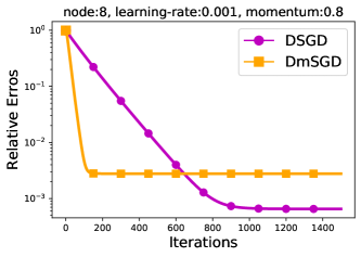
Figure 2: Convergence comparison between DSGD and DmSGD for a full-batch linear regression problem. Detailed experimental setting is in Appendix G.2.

DmSGD’s inconsistency bias: magnitude. The following proposition quantitatively evaluates the magnitude of DmSGD’s inconsistency bias. We let $\rho=\max\{|\lambda_{2}(W)|,|\lambda_{n}(W)|\}$, which characterize how well the network is connected. Since $W$ is doubly stochastic (Assumption A.3), it holds that $\rho\in(0,1)$ (see Appendix A). A well connected network will have $\rho\to 0$.

Proposition 2.

Under Assumptions A.1 and A.3, if each $f_{i}(x)$ is further assumed to be strongly-convex, and the full-batch gradient $\nabla f_{i}(x)$ is accessed per iteration, then DmSGD (6) has the following inconsistency bias:

$$\lim_{k\to\infty}\sum_{i=1}^{n}\|x_{i}^{(k)}-x^{\star}\|^{2}=O\Big{(}\frac{\gamma^{2}b^{2}}{(1-\beta)^{2}(1-\rho)^{2}}\Big{)},$$ (7)

where $b^{2}=(1/n)\sum_{i=1}^{n}\|\nabla f_{i}(x^{\star})\|^{2}$ denotes the data inconsistency between nodes, and $\beta$ is the momentum coefficient. (Proof is in Appendix C.2)

Note that we do not take expectation over $\sum_{i=1}^{n}\|x_{i}^{(k)}-x^{\star}\|^{2}$ in (7) because no gradient noise exists in recursion (6). Recall from Appendix C.1 that DSGD has an inconsistency bias on the order of $O(\gamma^{2}b^{2}/(1-\rho)^{2})$. Comparing it with (7), it is observed that the momentum term in DmSGD is essentially amplifying the inconsistency bias by a margin of $1/(1-\beta)^{2}$. This can explain why DmSGD converges less accurate than DSGD as illustrated in Fig. 2. Noting that $\beta$ is typically set close to $1$ in practice, DmSGD can suffer from a significantly large inconsistency bias. Since inconsistency bias dominates the large-batch scenario (see Proposition 1), DmSGD is thus observed to have severely deteriorated performance as illustrated in Table 1.

5 Improving Inconsistency Bias: DecentLaM

To improve large-batch DmSGD’s accuracy, we have to reduce the influence of momentum on inconsistency bias.

DSGD interprets as standard SGD. Without loss of generality, we assume each node $i$ can access the accurate gradient $\nabla f_{i}(x)$ in DSGD recursions (4)–(5). In this scenario, DSGD can be rewritten into a compact form:

$${\mathbf{x}}^{(k+1)}=W\big{(}{\mathbf{x}}^{(k)}-\gamma\nabla f({\mathbf{x}}^{(k)})\big{)}.$$ (8)

To simplify the derivation, we assume the weight matrix $W$, in addition to satisfying Assumption A.3, is positive-definite. With this assumption, $W$ can be eigen-decomposed into $W=U\Lambda U^{T}$ where $U$ is an orthogonal matrix and $\Lambda$ is a positive definite matrix. We define $W^{\frac{1}{2}}=U\Lambda^{\frac{1}{2}}U^{T}$ so that $W^{\frac{1}{2}}$ is also positive-definite and $W=W^{\frac{1}{2}}\times W^{\frac{1}{2}}$. We next introduce ${\mathbf{x}}=W^{\frac{1}{2}}{\mathbf{s}}$ and hence ${\mathbf{s}}=W^{-\frac{1}{2}}{\mathbf{x}}$. Left-multiplying $W^{-\frac{1}{2}}$ to both sides of (8),

$${\mathbf{s}}^{(k+1)} =W{\mathbf{s}}^{(k)}-\gamma W^{\frac{1}{2}}\nabla f(W^{\frac{1}{2}}{\mathbf{s}}^{(k)})$$

$$=W{\mathbf{s}}^{(k)}-\gamma\nabla_{{\mathbf{s}}}f(W^{\frac{1}{2}}{\mathbf{s}}^{(k)})$$

$$={\mathbf{s}}^{(k)}-\gamma\big{(}\nabla_{{\mathbf{s}}}f(W^{\frac{1}{2}}{\mathbf{s}}^{(k)})+\frac{1}{\gamma}(I-W){\mathbf{s}}^{(k)}\big{)}$$ (9)

In other words, DSGD (8) (with constant $\gamma$) can be interpreted as a standard SGD (9) (in terms of ${\mathbf{s}}$) to solve:

$$\min_{{\mathbf{s}}}\quad f(W^{\frac{1}{2}}{\mathbf{s}})+\frac{1}{2\gamma}\|{\mathbf{s}}\|^{2}_{I-W},$$ (10)

and ${\mathbf{x}}^{(k)}$ can be achieved by ${\mathbf{x}}^{(k)}=W^{\frac{1}{2}}{\mathbf{s}}^{(k)}$ per iteration. When recursion (9) approaches the solution ${\mathbf{s}}^{o}$ to problem (10), DSGD (8) will achieve the fixed point ${\mathbf{x}}^{o}=W^{\frac{1}{2}}{\mathbf{s}}^{o}$. The inconsistency bias of DSGD is essentially the distance between ${\mathbf{x}}^{o}$ and ${\mathbf{x}}^{\star}=[x^{\star},\cdots,x^{\star}]\in{\mathbb{R}}^{n\times d}$ where $x^{\star}$ is the global solution to problem (1). Since ${\mathbf{x}}^{o}\neq{\mathbf{x}}^{\star}$, such inconsistency bias generally exists in DSGD.

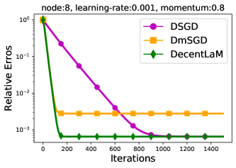
Figure 3: Convergence comparison between DSGD, DmSGD and decentLaM for a full-batch linear regression problem.

Remark 1.

The interpretation of DSGD (8), which is usually named as the adaptation-then-combination (ATC) version of DSGD, as standard SGD (9) is novel. Existing literatures [57, 4] can bridge the adaptation-with-combination (AWC) version of DSGD, i.e., ${\mathbf{x}}^{(k+1)}=W{\mathbf{x}}^{(k)}-\gamma\nabla f({\mathbf{x}}^{(k)})$, with standard SGD, but not for ATC-DSGD. ATC-DSGD can enable larger learning rates and has a better convergence performance than AWC-DSGD [41, Secs. 10.6 and 11.5], [59, 23], and is hence more widely used in deep training [25, 3, 46, 55, 13, 43, 26, 20].

DecentLaM development. It is established in Proposition 2 that the momentum term in DmSGD can significantly amplify the inconsistency bias especially when $\beta\to 1$. This section proposes DecentLaM to remove the negative influence of momentum in DmSGD.

Since DSGD can be interpreted as a standard SGD, we can easily integrate it to the existing momentum acceleration techniques [32, 58, 14, 30, 55]. By letting ${\mathbf{g}}_{s}^{(k)}$ be the standard gradient of problem (10) at iteration $k$, the standard momentum SGD approach to solving problem (10) is

$${\mathbf{g}}_{s}^{(k)} =\nabla_{{\mathbf{s}}}f(W^{\frac{1}{2}}{\mathbf{s}}^{(k)})+\frac{1}{\gamma}(I-W){\mathbf{s}}^{(k)}$$ (11)

$${\mathbf{m}}^{(k+1)}_{s} =\beta{\mathbf{m}}^{(k)}_{s}+{\mathbf{g}}_{s}^{(k)}$$ (12)

$${\mathbf{s}}^{(k+1)} ={\mathbf{s}}^{(k)}-\gamma{\mathbf{m}}^{(k+1)}_{s}$$ (13)

After achieving ${\mathbf{s}}^{(k+1)}$, we get ${\mathbf{x}}^{(k+1)}=W^{\frac{1}{2}}{\mathbf{s}}^{(k+1)}$. Recursions (11)–(13) are named as DecentLaM, and we simulate their convergence behaviour under the same setting as in Fig. 2. It is observed in Fig. 3 that the proposed algorithm converges as fast as DmSGD but to a more accurate solution. Since DecentLaM is with an improved inconsistency bias, it better fits into the large-batch scenario.

Efficient implementation. To apply DecentLaM (11)-(13) to train deep neural networks, we need two additional modifications: (i) the full-batch gradient $\nabla f_{i}(x)$ needs to be replaced with the stochastic gradient $\nabla F(x;\xi_{i})$; (ii) the matrix $W^{\frac{1}{2}}$ should be removed from the algorithm update. To this end, by letting ${\mathbf{g}}=W^{\frac{1}{2}}{\mathbf{g}}_{s}$, ${\mathbf{m}}=W^{\frac{1}{2}}{\mathbf{m}}_{s}$, and $\tilde{{\mathbf{g}}}$ be the stochastic version of ${\mathbf{g}}$, (11)-(13) can be rewritten as

$$\tilde{{\mathbf{g}}}^{(k)} =W\nabla F({\mathbf{x}}^{(k)};{\boldsymbol{\xi}}^{(k)})+\frac{1}{\gamma}(I-W){\mathbf{x}}^{(k)}$$ (14)

$${\mathbf{m}}^{(k+1)} =\beta{\mathbf{m}}^{(k)}+\tilde{{\mathbf{g}}}^{(k)}$$ (15)

$${\mathbf{x}}^{(k+1)} ={\mathbf{x}}^{(k)}-\gamma{\mathbf{m}}^{(k+1)}$$ (16)

where we have replaced $\nabla f({\mathbf{x}}^{(k)})$ with $\nabla F({\mathbf{x}}^{(k)};{\boldsymbol{\xi}}^{(k)})$ in (14) to enable the usage of stochastic gradient. The above algorithm is almost the same as the vanilla momentum SGD within a single computing node, with the exception to construct ${\mathbf{g}}^{(k)}$ as in (14). The decentralized implementation of (14)-(16) is listed in Algorithm 2, where

$$\tilde{g}_{i}^{(k)}=\frac{1}{\gamma}x_{i}^{(k)}-\frac{1}{\gamma}\sum_{j\in\mathcal{N}_{i}}w_{ij}\big{(}x_{j}^{(k)}-\gamma\nabla F(x_{j}^{(k)};\xi_{j}^{(k)})\big{)}.$$ (17)

The momentum update and local model update in Algorithm 2 can be conducted via the mSGD optimizer provided by PyTorch or TensorFlow. As shown in Fig. 4, the dashed part, which is different from the DmSGD workflow, enables an efficient wait-free backpropagation (WFBP) implementation that can overlap communication and computation.

Require: Initialize $\gamma$, $x^{(0)}_{i}$; let $m^{(0)}_{i}=0,\beta\in(0,1)$

for $k=0,1,2,...,T-1$, every node $i$ do

       Sample $\xi^{(k)}_{i}$ and update $\tilde{g}_{i}^{(k)}$ according to (17)

      

      $m^{(k+1)}_{i}=\beta m^{(k)}_{i}+\tilde{g}_{i}^{(k)}\hskip 17.07182pt\triangleright\mbox{\footnotesize{momentum update}}$

      

      $x^{(k+1)}_{i}=x^{(k)}_{i}-\gamma m^{(k+1)}_{i}\hskip 9.95863pt\triangleright\mbox{\footnotesize{local model update}}$

      

Algorithm 2 DecentLaM

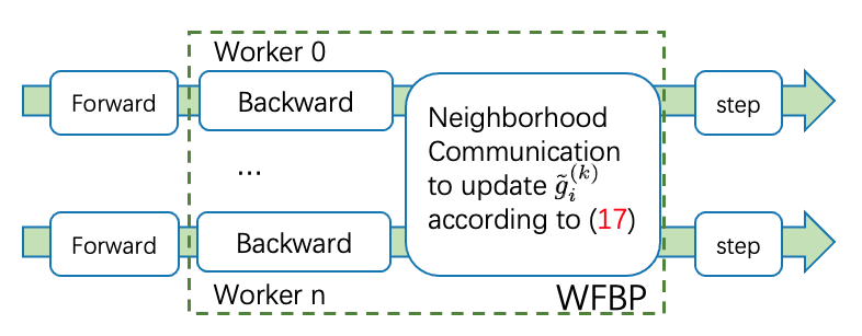
Figure 4: The workflow of DecentLaM in a training iteration.

DecentLaM’s inconsistency bias. The following proposition quantitatively evaluates the magnitude of DecentLaM’s inconsistency bias (Proof is in Appendix C.3):

Proposition 3.

Under the same assumptions as Proposition 2, DecentLaM has an inconsistency bias as follows:

$$\lim_{k\to\infty}\sum_{i=1}^{n}\|x_{i}^{(k)}-x^{\star}\|^{2}=O\Big{(}\frac{\gamma^{2}b^{2}}{(1-\rho)^{2}}\Big{)},$$ (18)

Remark 2.

Comparing with DmSGD’s inconsistency bias (7), it is observed that DecentLaM completely removes the negative effects of momentum; it improves DmSGD’s inconsistency bias by a margin of $1/(1-\beta)^{2}$. When $b^{2}$ is large or $\beta$ is close to $1$, such improvement is remarkable.

Remark 3.

Comparing with DSGD’s inconsistency bias $O(\gamma^{2}b^{2}/(1-\rho)^{2})$, it is observed that DecentLaM has exactly the same inconsistency bias as DSGD. However, the momentum term in DecentLaM will significantly speed up its convergence rate. The simulation results in Fig. 3 are consistent with the conclusions discussed in Remarks 2-3.

6 Convergence analysis of DecentLaM

Sec. 5 proposes a novel algorithm DecentLaM and explains why it better fits into the large-batch scenario. This section establishes the formal convergence analysis in the non-convex and strongly-convex scenarios, respectively.

6.1 Non-convex scenario

We introduce a standard data inconsistency assumption for the non-convex scenario:

Assumption A.4 There exits a constant $\hat{b}>0$ such that $\frac{1}{n}\sum_{i=1}^{n}\|\nabla f_{i}(x)-\nabla f(x)\|^{2}\leq\hat{b}^{2}$ for any $x$, where $f(x)$ is the global cost function defined in (1).

Assumption A.4 is much more relaxed than the commonly used assumption that each $\nabla f_{i}(x)$ is upper bounded (i.e., $\|\nabla f_{i}(x)\|\leq M$) [13, 43, 4]. When data distribution $D_{i}$ in each computing node $i$ is identical to each other, it holds that $f_{i}(x)=f_{j}(x)$ for any $i$ and $j$, which implies $\hat{b}=0$.

Theorem 1.

Under Assumptions A.1–A.4, if learning rate $\gamma=\min\{\frac{(1-\beta)^{2}}{5\sqrt{\beta+\beta^{2}}L},\frac{(1-\beta)^{2}}{(5-\beta+2\beta^{2})L},\frac{(1-\beta)^{2}}{12L\beta^{2}},\frac{1-\rho}{20\sqrt{\rho}L}\}$, $W$ is positive-definite, and $\beta+\frac{16\beta^{2}}{(1-\beta)(1-\rho)^{2}}\leq\frac{3+\rho}{4}$, the DecentLaM algorithm in Algorithm 2 will converge as follows (Proof is in Appendix E, and $\bar{x}^{(k)}=\frac{1}{n}\sum_{i=1}^{n}x_{i}^{(k)}$):

$$\frac{1}{T}\sum_{k=0}^{T-1}\mathbb{E}\|\frac{1}{n}\sum_{i=1}^{n}\nabla f_{i}(\bar{x}^{(k)})\|^{2}$$ (19)

$$= O\Big{(}\underbrace{\frac{1-\beta}{\gamma T}}_{\rm convg.\ rate}+\underbrace{\frac{\gamma\sigma^{2}}{n(1-\beta)}+\frac{\gamma^{2}\sigma^{2}}{1-\rho}}_{\rm sto.\ bias}+\underbrace{\frac{\gamma^{2}\hat{b}^{2}}{(1-\rho)^{2}}}_{\rm inconsist.bias}\Big{)}$$

Expression (19) indicates that DecentLaM will converge sublinearly to a limiting bias. The limiting bias (which can be achieved by letting $T\to\infty$) can be separated into the stochastic bias and the inconsistency bias, which is consistent with our discussion in Sec. 1. It is also observed that the inconsistency bias term in (19) is unrelated to the momentum coefficient $\beta$, which implies, as discussed in Sec. 5, that DecentLaM has removed the negative affects of momentum. Theorem 1 has restrictions on the positive-definiteness of $W$ and the momentum parameter $\beta$ so that the analysis can be simplified. However, they are not needed in the real practice and not used in any of our experiments in Sec. 7. We find the concurrent work [26] also imposes a restriction on momentum parameter to simply the analysis.

Corollary 1.

Under the same assumptions as in Theorem 1, if learning rate $\gamma=O((1-\beta)/\sqrt{T/n})$, DecentLaM will converge at rate $O(1/\sqrt{nT})$ (Proof is in Appendix E), which achieves the same linear speedup as PmSGD.

6.2 Strongly-convex scenario

Assumption A.5 Each $f_{i}(x)$ is $\mu$-strongly convex, i.e., $\langle\nabla f_{i}(x)-\nabla f_{i}(y),x-y\rangle\geq\mu\|x-y\|^{2}$ for any $x,y\in\mathbb{R}^{d}$.

Under Assumption A.5, the global solution to problem (1) is unique. Furthermore, we do need to make the data heterogeneity assumption A.4 in the strongly-convex scenario. Instead, we will use $b^{2}=\frac{1}{n}\sum_{i=1}^{n}\|\nabla f_{i}(x^{\star})\|^{2}$ to gauge the data heterogeneity

Theorem 2.

Under Assumption A.1–A.3 and A.5, if $\gamma=\min\{\frac{(1-\beta)^{2}}{27L},\frac{(1-\rho)(1-\beta)(\kappa+1)}{5L},\frac{1-\rho}{\sqrt{1728(\kappa+1)}}\}$, $W$ is positive definite, and $\beta+\frac{16\beta^{2}}{(1-\beta)(1-\rho)^{2}}\leq\frac{3+\rho}{4}$, DecentLaM in Algorithm 2 will converge as (Proof is in Appendix F):

$$\ \frac{1}{nH_{T}}\sum_{k=0}^{T}\sum_{i=1}^{n}h_{k}(\mathbb{E}f_{i}(\bar{x}^{(k)})-f^{*})$$

$$= O\Big{(}\underbrace{\frac{(1-\beta)}{\gamma}(1-\frac{\gamma}{(1-\beta)})^{T}}_{\rm convg.\ rate}$$

$$\quad+\underbrace{\frac{\gamma\sigma^{2}}{n(1-\beta)}+\frac{\gamma^{2}\sigma^{2}}{1-\rho}}_{\rm sto.\ bias}+\underbrace{\frac{\gamma^{2}{b}^{2}}{(1-\rho)^{2}}}_{\rm inconsist.bias}\Big{)}$$ (20)

where $h_{k}$ is some positive weight (see Appendix F) and $H_{T}=\sum_{k=0}^{T}h_{k}$. Quantity $f^{\star}=\min_{x}f(x)$.

The inconsistency bias in (2) is independent of the momentum $\beta$, which is consistent with Proposition 3 . It implies that DecentLaM achieves the same $O(\gamma^{2}b^{2}/(1-\rho)^{2})$ inconsistency bias as DSGD (see (38)).

Theorem 2 establishes the convergence of DecentLaM with a constant learning rate. When learning rate is decaying, DecentLaM converges exactly to the global solution:

Corollary 2.

Under the same assumptions as Theorem 2, if learning rate $\gamma={O}(\frac{(1-\beta)\ln(nT^{2})}{T})$, DecentLaM will converge as follows (Proof is in Appendix F):

$$\frac{1}{nH_{T}}\sum_{k=0}^{T}\sum_{i=1}^{n}h_{k}(\mathbb{E}f_{i}(\bar{x}^{(k)})-f^{*})=\tilde{O}\Big{(}\frac{1}{nT}\Big{)}$$ (21)

where $\tilde{O}(\cdot)$ hides all logarithm factors.

Corollary 2 implies that DecentLaM achieves the same linear speedup as PmSGD in the strongly-convex scenario [30]. However, it saves more communication per iteration due to the partial averaging (see Sec. 3).

6.3 Comparison with existing methods

As we discussed in Sec. 1, the inconsistency bias will dominate the convergence performance as batch-size gets large. For this reason, we list the inconsistency bias comparison between DecentLaM and existing DmSGD variants in Table 2. By removing the influence of momentum, DecentLaM has the smallest inconsistency bias. This implies DecentLaM can perform better in the large-batch scenario.

	Strongly-convex	Non-convex
DmSGD [13]	N.A.	$O\big{(}\frac{\gamma^{2}M^{2}}{(1-\beta)^{2}}\big{)}$
DmSGD [43]	$O\big{(}\frac{\gamma^{5/2}M^{2}}{(1-\beta)^{6}}\big{)}$	$O\big{(}\frac{\gamma^{2}M^{2}}{(1-\beta)^{4}}\big{)}$
DmSGD (eq.(7))	$O\big{(}\frac{\gamma^{2}b^{2}}{(1-\beta)^{2}}\big{)}$	N.A
DA-DmSGD [55]	N.A.	$O\big{(}\frac{\gamma^{2}\hat{b}^{2}}{(1-\beta)^{2}}\big{)}$
AWC-DmSGD [4]	$O\big{(}\frac{\gamma^{2}M^{2}}{(1-\beta)^{2}}\big{)}$	$O\big{(}\frac{\gamma^{2}M^{2}}{(1-\beta)^{4}}\big{)}$
SlowMo [49]	N.A	N.A
DecentLaM (Ours)	$\boldsymbol{O(\gamma^{2}b^{2})}$	$\boldsymbol{O(\gamma^{2}\hat{b}^{2})}$

Table 2: Inconsistency bias comparison between various decentralized momentum algorithms. Constant $M$ is the gradient’s upper bound, which is typically much larger than the data inconsistency $b$ or $\hat{b}$. SlowMo [49] only examined the data-homogeneous scenario. It did not clarify what the inconsistency bias is.

After completing this work, we become aware of the concurrent work QG-DmSGD [26] that can also achieve $O(\gamma^{2}\hat{b}^{2})$ for non-convex scenario. However, QG-DmSGD is based on a strategy to mimic the global momentum, which is different from the core idea to develop DecentLaM. Furthermore, QG-DmSGD is designed for highly data-heterogeneous scenario in EdgeAI applications while DecentLaM is for large-batch training within data-centers. As a result, our experimental tasks and algorithm settings are very different. In addition, our analysis is also different from QG-DmSGD. With a delicately designed Lyapunov function, we can cover the convergence analysis for both non-convex and strongly-convex scenarios. In contrast, the analysis in QG-DmSGD is for the non-convex scenario. Finally, we theoretically uncovered the reason why traditional DmSGD [55, 13, 43] has degraded performance in Sec. 1 while QG-DmSGD only justifies it empirically.

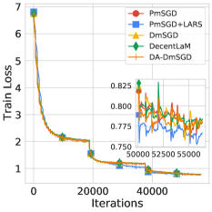
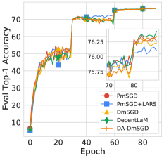
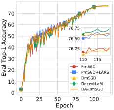
Figure 5: Convergence results on the ImageNet with respect to training loss and validation top-1 accuracy. The batch size is 2k for left-side two figures and 16k for right-side two figures. For clarity, we do not depict the curves of other baselines.

7 Experiments

In this section, we systematically compare the proposed method, DecentLaM, with well-known state-of-the-art methods on typical large-scale computer vision tasks: image classification and object detection. In particular, we compare DecentLaM with the following algorithms. PmSGD is the standard Parallel momentum SGD algorithm in which a global synchronization across all nodes are required per iteration. PmSGD + LARS exploits a layer-wise adaptive rate scaling strategy [51] to boost performance with large batch-size. DmSGD [3, 13, 43] exploits partial averaging to save communications. Its recursions are listed in Algorithm 1. DA-DmSGD [55] incurs additional partial averaging over the momentum to increase stability; it has double partial averages per iteration. AWC-DmSGD [4] accelerates AWC-DSGD with momentum. SlowMo [49] periodically synchronize each node and adds an additional slow momentum update. QG-DmSGD [26] is a concurrent work to DecentLaM that adds a quasi-global momentum to DSGD. We utilize the QG-DmSGD Heavy-ball variant. D² [46] is a primal-dual approach that can completely remove the inconsistency bias theoretically. The vanilla D² algorithm does not perform well in our experiments. We refer to another form of D² in [56] and add momentum acceleration to the local update step. We name this algorithm as D²-DmSGD. All baseline algorithms are tested with the recommended hyper-parameters in their papers. Note that DecentLaM requires symmetric (but not necessarily positive definite) weight matrix to guarantee empirical convergence.

We implement all the aforementioned algorithms with PyTorch [36] 1.6.0 using NCCL 2.8.3 (CUDA 10.2) as the communication backend. For PmSGD, we used PyTorch’s native Distributed Data Parallel (DDP) module. For the implementation of decentralized methods, we utilize BlueFog [1], which is a high-performance decentralized deep training framework, to facilitate the topology organization, weight matrix generation, and efficient partial averaging. We also follow DDP’s design to enable computation and communication overlap. Each server contains 8 V100 GPUs in our cluster and is treated as one node. The inter-node network fabrics are 25 Gbps TCP as default, which is a common distributed training platform setting. To eliminate the effect of topology with different size in decentralized algorithms, we used 8 nodes (i.e. $8\times 8=64$ GPUs) in all decentralized training and changed the batch size of every single GPU respectively.

7.1 Image Classification

method	Batch Size
	2k	8k	16k	32k
PmSGD	76.32	76.08	76.27	75.27
PmSGD+LARS[51]	76.16	75.95	76.65	75.63
DmSGD[3, 13, 43]	76.27	76.01	76.23	74.97
DA-DmSGD[55]	76.35	$\mathbf{76.19}$	76.62	75.51
AWC-DmSGD[4]	76.29	75.96	76.31	75.37
SlowMo[49]	76.30	75.47	75.53	75.33
QG-DmSGD[26]	76.23	75.96	76.60	75.86
D2-DmSGD[46]	75.44	75.30	76.16	75.44
DecentLaM (Ours)	$\mathbf{76.43}$	$\mathbf{76.19}$	$\mathbf{76.73}$	$\mathbf{76.22}$

Table 3: Top-1 validation accuracy of aforementioned methods when training ResNet-50 model with different batch sizes.

Implementation. We conduct a series of image classification experiments with the ImageNet-1K [10] dataset, which consists of 1,281,167 training images and 50,000 validation images in 1000 classes. We train classification models with different batch sizes to verify our theoretical findings. As suggested in [15], we treat batch size equal or less than 8k as small-batch setting and the training protocol in [15] is used. In details, we train total 90 epochs. The learning rate is warmed up in the first 5 epochs and is decayed by a factor of 10 at 30, 60 and 80 epochs. For large-batch setting (batch size larger than 8K), we train total 120 epochs. The learning rate is warmed up in the first 20 epochs and is decayed in a cosine annealing scheduler as suggested in [52]. The choice of hyper-parameter setting is not cherry-picked and we try to keep our PmSGD’s baseline around 76% while [15]’s setting has severe performance drop even for large-batch PmSGD. The momentum SGD optimizer is with linear scaling by default. Experiments are trained in the mixed precision using Pytorch native amp module.

model	ResNet-18			ResNet-34			ResNet-50			MobileNet-v2			EfficientNet
Batch Size	2k	8k	16k	2k	8k	16k	2k	8k	16k	2k	8k	16k	2k	8k	16k
PmSGD	70.0	69.5	68.3	$\mathbf{73.8}$	72.8	72.9	76.3	76.1	76.3	70.6	71.1	69.5	77.6	77.0	78.1
PmSGD+LARS	70.2	69.9	$\mathbf{70.6}$	73.6	$\mathbf{73.2}$	73.3	76.2	76.0	$\mathbf{76.7}$	70.7	71.3	$\mathbf{72.3}$	77.7	77.2	78.2
DmSGD	69.9	69.3	68.7	73.1	72.7	72.4	76.3	76.0	76.2	70.5	71.0	72.1	77.5	76.9	77.5
DA-DmSGD	70.2	70.0	70.2	73.3	73.1	73.1	$\mathbf{76.4}$	$\mathbf{76.2}$	76.6	70.4	$\mathbf{71.4}$	72.1	77.6	$\mathbf{77.4}$	77.8
AWC-DmSGD	69.5	69.4	70.4	73.2	72.7	73.2	76.3	76.0	76.3	70.6	70.8	71.9	77.4	76.9	77.7
SlowMo	70.5	70.0	69.9	73.5	73.0	73.0	76.3	75.5	75.5	68.7	69.1	67.8	77.4	77.2	77.1
QG-DmSGD	70.2	$\mathbf{70.5}$	${70.3}$	$\mathbf{73.8}$	73.1	73.3	76.2	76.0	76.6	$\mathbf{70.8}$	70.6	72.0	76.8	76.5	76.7
D2-DmSGD	69.1	68.9	70.1	72.7	72.3	73.1	75.4	75.3	76.2	70.2	70.6	71.8	76.6	76.4	76.5
DecentLaM	$\mathbf{70.3}$	69.9	70.5	73.4	73.1	$\mathbf{73.4}$	$\mathbf{76.4}$	$\mathbf{76.2}$	$\mathbf{76.7}$	70.3	$\mathbf{71.4}$	72.2	$\mathbf{77.8}$	77.2	$\mathbf{78.3}$

Table 4: Top-1 validation accuracy comparison with different models and batch sizes on ImageNet dataset.

Performance with different batch-sizes. We first compare the top-1 accuracy of the aforementioned methods when training ResNet-50 [16] model ($\sim$25.5M parameters) with different batch-sizes on ImageNet. The network topology is set as the symmetric exponential topology (see G.3). The results are listed in Table 3. It is observed that:

• DecentLaM always has better accuracy than other decentralized algorithms, and its superiority gets evident as batch size grows. DecentLaM outperforms other baselines by a large margin in the 32K batch size scenario due to its improved inconsistency bias derived in Proposition 3, Theorems 2 and 1.

• DecentLaM even outperforms PmSGD and PmSGD + LARS for each batch-size. One conjecture is that its model inconsistency between nodes caused by the partial averaging helps the algorithm escape from shallow local minimums. As a result, DecentLaM can be better as well as faster than DmSGD (with LARS).

• DmSGD, DA/AWC-DmSGD, and SlowMo have a severe degraded performance in the 32K batch size scenario. It is because the momentum have amplified their inconsistency bias, see Proposition 2 and the results listed in Table 2. D²-DmSGD’s performance also drops significantly while it can theoretical remove all inconsistency bias. QG-DmSGD has relatively small performance degradation, but it still performs worse than DecentLaM.

We also depict the training loss and top-1 validation accuracy curves on ResNet-50 with 2K and 16K batch sizes in Fig. 5. When batch size is 2K, it is observed that DecentLaM achieves roughly the same training loss as DmSGD. However, as batch size grows to 16K, DecentLaM achieves visibly smaller training loss than DmSGD. This observation illustrates that DecentLaM improves inconsistency bias which can boost its convergence when batch-size is large.

topology	Batch Size
	16k	32k
Ring	76.65	76.34
Mesh	76.54	76.47
Symmetric Exponential	76.73	76.22
bipartite random match	76.53	76.11

Table 5: DecentLaM has consistent performance with different network topologies on ImageNet (ResNet-50).

Performance with different models. We now validate whether DecentLaM is effective to different neural network architectures. Table 4 compares the top-1 accuracy with backbones widely-used in image classification tasks including ResNet [16], MobileNetv2 [40] and EfficientNet [45]. The accuracy of PmSGD is slightly different from those reported in [40, 45] because we do not utilize tricks such as AutoAugment [9] that are orthogonal to our methods. It is observed in Table 4 that either PmSGD + LARS or DecentLaM achieves best performance with large batch-size (16K) across different models. However, DecentLaM has runtime speedup due to its efficient neighborhood-communication. For small-batch settings, DA-DmSGD and QG-DmSGD can also achieve the best accuracy for some models.

Performance with different topologies. We now examine how DecentLaM is robust to different topologies. To this end, we first organize all computing nodes into ring, mesh, symmetric exponential, or the bipartite random match topology, see Appendix G.3 for details of these topologies. Next we test the performance of DecentLaM on ResNet-50 with these topologies and the results are in Table 5. It is observed that DecentLaM has a consistent performance with different topologies. The ring topology is sparser than symmetric exponential topology. Interestly, it is observed to have a better accuracy in the 32K batch-size setting. It is conjectured that the ring topology can help escape from shallow local minimums when batch-size is large. We leave the justification as the future work.

Training time comparison. The end-to-end training speed varies across different models and network bandwidth conditions. For the sake of brevity, we compare the runtime of PmSGD, DmSGD and DecentLaM in training ResNet-50 (ImageNet) with different batch sizes and network bandwidths. The speed-up of DmSGD/DecentLaM over PmSGD is consistent for other backbones and tasks. In Fig. 6, DecentLaM and DmSGD have equivalent runtime because they are based on the same partial averaging operation. However, they can achieve 1.2$\sim$1.9$\times$speed-up compared to PmSGD, which is consistent with [3].

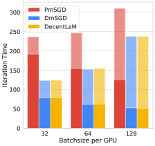
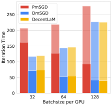
Figure 6: Runtime comparison on ResNet-50 with different batch sizes and network bandwidth (Left: 10Gbps; Right: 25Gbps). Each column indicates the averaged iteration runtime of 500 iterations. The thick part highlights the communication overhead.

7.2 Object Detection

We compared the aforementioned methods with well-known detection models, e.g. Faster-RCNN [39] and RetinaNet [28] on popular PASCAL VOC [12] and COCO [29] datasets. We adopt the MMDetection [7] framework as the building blocks and utilize ResNet-50 with FPN [27] as the backbone network. We choose mean Average Precision (mAP) as the evaluation metric for both datesets. We used 8 GPUs (which are connected by the symmetric exponential topology) and set the total batch size as 256 in all detection experiments. Table 6 shows the performance of each algorithm. Compared with classification tasks, the total batch size in object detection cannot be set too large (typical object detection task sets batch size as $2$ within each GPU). For this reason, our proposed method just reaches a slightly higher mAP than other methods.

Dataset	PASCAL VOC		COCO
Model	R-Net	F-RCNN	R-Net	F-RCNN
PmSGD	79.0	80.3	36.2	36.5
PmSGD+LARS	78.5	79.8	35.7	36.2
DmSGD	79.1	80.5	36.1	36.4
DA-DmSGD	79.0	80.5	36.4	37.0
DecentLaM	$\mathbf{79.3}$	$\mathbf{80.7}$	$\mathbf{36.6}$	$\mathbf{37.1}$

Table 6: Comparision of aforementioned methods with different models on PASCAL VOC and COCO datasets. R-Net and F-RCNN refer to RetinaNet and Faster-RCNN respectively.

8 Conclusion

We investigated the performance degradation in large-batch DmSGD and proposed DecentLaM to remove the momentum-incurred bias. Theoretically, we demonstrate the convergence improvement in smooth convex and non-convex scenarios. Empirically, experimental results of various models and tasks validate our theoretical findings.

Appendix A Preliminary

Notation. We first introduce necessary notations as follows.

• ${\mathbf{x}}^{(k)}=[(x_{1}^{(k)})^{T};(x_{2}^{(k)})^{T};\cdots;(x_{n}^{(k)})^{T}]\in\mathbb{R}^{n\times d}$

• $\nabla F({\mathbf{x}}^{(k)};{\boldsymbol{\xi}}^{(k)})=[\nabla F_{1}(x_{1}^{(k)};\xi_{1}^{(k)})^{T};\cdots;\nabla F_{n}(x_{n}^{(k)};\xi_{n}^{(k)})^{T}]\in\mathbb{R}^{n\times d}$

• $\nabla f({\mathbf{x}}^{(k)})=[\nabla f_{1}(x_{1}^{(k)})^{T};\nabla f_{2}(x_{2}^{(k)})^{T};\cdots;\nabla f_{n}(x_{n}^{(k)})^{T}]\in\mathbb{R}^{n\times d}$

• $f({\mathbf{x}}^{(k)})=\sum_{i=1}^{n}f(x_{i}^{(k)})$ and $f(x^{(k)})=\sum_{i=1}^{n}f(x^{(k)})$

• $\bar{{\mathbf{x}}}^{(k)}=[(\bar{x}^{(k)})^{T};(\bar{x}^{(k)})^{T};\cdots;(\bar{x}^{(k)})^{T}]\in\mathbb{R}^{n\times d}$ where $\bar{x}^{(k)}=\frac{1}{n}\sum_{i=1}^{n}{\boldsymbol{x}}_{i}^{(k)}$

• ${{\mathbf{x}}}^{\star}=[({x}^{\star})^{T};({x}^{\star})^{T};\cdots;({x}^{\star})^{T}]\in\mathbb{R}^{n\times d}$ where ${x}^{\star}$ is the global solution to problem (1).

• $W=[w_{ij}]\in\mathbb{R}^{n\times n}$ is the weight matrix.

• $\mathds{1}_{n}=\mathrm{col}\{1,1,\cdots,1\}\in{\mathbb{R}}^{n}$.

• Given two matrices ${\mathbf{x}},{\mathbf{y}}\in{\mathbb{R}}^{n\times d}$, we define inner product $\langle{\mathbf{x}},{\mathbf{y}}\rangle=\mathrm{tr}({\mathbf{x}}^{T}{\mathbf{y}})$, the Frobenius norm $\|{\mathbf{x}}\|^{2}=\langle{\mathbf{x}},{\mathbf{x}}\rangle$, and the $\|{\mathbf{x}}\|_{2}$ as ${\mathbf{x}}$’s $\ell_{2}$ norm. Furthermore, for a positive semi-definite matrix $A\in{\mathbb{R}}^{n\times n}$, we define $\langle{\mathbf{x}},{\mathbf{y}}\rangle_{A}=\mathrm{tr}({\mathbf{x}}^{T}A{\mathbf{y}})$ and $\|{\mathbf{x}}\|^{2}_{A}=\langle{\mathbf{x}},{\mathbf{x}}\rangle_{A}$ for simplicity.

• Given $W\in{\mathbb{R}}^{n\times n}$, we let $\|W\|_{2}=\sigma_{\max}(W)$ where $\sigma_{\max}(\cdot)$ denote the maximum sigular value.

GmSGD in matrix notation. For ease of analysis, we rewrite the recursion of GmSGD in Algorithm 1 with matrix notation:

$${\mathbf{m}}^{(k+1)} =\beta{\boldsymbol{m}}^{(k)}+\nabla F({\mathbf{x}}^{(k)};{\boldsymbol{\xi}}^{(k)})$$ (22)

$${\mathbf{x}}^{(k+1)} =W({\mathbf{x}}^{(k)}-\gamma{\mathbf{m}}^{(k+1)})$$ (23)

DecentLaM in matrix notation. We can also rewrite DecentLaM in Algorithm 2 with matrix notation:

$$\tilde{{\mathbf{g}}}^{(k)} =\frac{1}{\gamma}{\mathbf{x}}^{(k)}-\frac{1}{\gamma}W({\mathbf{x}}^{(k)}-\gamma\nabla F({\mathbf{x}}^{(k)},{\boldsymbol{\xi}}^{(k)}))$$ (24)

$${\mathbf{m}}^{(k+1)} =\beta{\mathbf{m}}^{(k)}+\tilde{{\mathbf{g}}}^{(k)}$$ (25)

$${\mathbf{x}}^{(k+1)} ={\mathbf{x}}^{(k)}-\gamma{\mathbf{m}}^{(k+1)}$$ (26)

Moreover, we define ${\mathbf{g}}^{(k)}=\mathbb{E}[\tilde{{\mathbf{g}}}^{(k)}]=\frac{1}{\gamma}{\mathbf{x}}^{(k)}-\frac{1}{\gamma}W({\mathbf{x}}^{(k)}-\gamma\nabla f({\mathbf{x}}^{(k)}))$

Smoothness. Since each $f_{i}(x)$ is assumed to be $L$-smooth in Assumption A.1, it holds that $f(x)=\frac{1}{n}\sum_{i=1}^{n}f_{i}(x)$ is also $L$-smooth. As a result, the following inequality holds for any $x,y\in\mathbb{R}^{d}$:

$$f(x)-f(y)-\frac{L}{2}\|x-y\|^{2} \leq\langle\nabla f(y),x-y\rangle$$ (27)

Network weight matrix. Suppose a symmetric matrix $W\in{\mathbb{R}}^{n\times n}$ satisfies Assumption A.3, and $\lambda_{j}$ denotes its $j$-th largest eigenvalue. It holds that $1=\lambda_{1}>\lambda_{2}\geq\cdots\geq\lambda_{n}>-1$. As a result, it holds that

$$\|W\|_{2}=1,\quad\mbox{and}\quad\rho=\|W-\frac{1}{n}\mathds{1}\mathds{1}^{T}\|_{2}=\max\{|\lambda_{2}|,|\lambda_{n}|\}\in(0,1)$$ (28)

If $W$ satisfying Assumption A.3 is further assumed to be positive-definite, it holds that $1=\lambda_{1}>\lambda_{2}\geq\cdots\geq\lambda_{n}>0$.

Submultiplicativity of the Frobenius norm. Given matrices $W\in{\mathbb{R}}^{n\times n}$ and ${\mathbf{y}}\in{\mathbb{R}}^{n\times d}$, it holds that

$$\|W{\mathbf{y}}\|\leq\|W\|_{2}\|{\mathbf{y}}\|.$$ (29)

To verify it, by letting $y_{j}$ be the $j$-th column of ${\mathbf{y}}$, we have $\|W{\mathbf{y}}\|^{2}=\sum_{j=1}^{d}\|Wy_{j}\|_{2}^{2}\leq\sum_{j=1}^{d}\|W\|_{2}^{2}\|y_{j}\|_{2}^{2}=\|W\|_{2}^{2}\|{\mathbf{y}}\|^{2}$.

Appendix B Reformulation of DmSGD and DecentLaM

B.1 Reformulation of DmSGD

In this section we show how DmSGD algorithm 1 can be rewritten as (6). To this end, we rewrite (23) as

$$\beta{\mathbf{x}}^{(k)}=W(\beta{\mathbf{x}}^{(k-1)}-\gamma\beta{\mathbf{m}}^{(k)}).$$ (30)

Subtracting (30) from (23), we have

$${\mathbf{x}}^{(k+1)}-\beta{\mathbf{x}}^{(k)}=W\big{(}{\mathbf{x}}^{(k)}-\beta{\mathbf{x}}^{(k-1)}-\gamma({\mathbf{m}}^{(k+1)}-\beta{\mathbf{m}}^{(k)})\big{)}\overset{\eqref{dmssgd-matrix-1}}{=}W\big{(}{\mathbf{x}}^{(k)}-\beta{\mathbf{x}}^{(k-1)}-\gamma\nabla F({\mathbf{x}}^{(k)};{\boldsymbol{\xi}}^{(k)})\big{)}$$ (31)

which is equivalent to

$${\mathbf{x}}^{(k+1)}=\underbrace{W\big{(}{\mathbf{x}}^{(k)}-\gamma\nabla F({\mathbf{x}}^{(k)};{\boldsymbol{\xi}}^{(k)})\big{)}}_{\rm DSGD}+\underbrace{\beta({\mathbf{x}}^{(k)}-W{\mathbf{x}}^{(k-1)})}_{\rm momentum}.$$ (32)

When a full-batch gradient is used, the above recursion becomes

$${\mathbf{x}}^{(k+1)}={W\big{(}{\mathbf{x}}^{(k)}-\gamma\nabla f({\mathbf{x}}^{(k)})\big{)}}+\beta({\mathbf{x}}^{(k)}-W{\mathbf{x}}^{(k-1)})$$ (33)

which is essentially recursion (6) in the matrix notation.

B.2 Reformulation of DecentLaM

In this section we show another formulation of DecentLaM Algorithm 2. To this end, we rewrite (26) as

$$\beta{\mathbf{x}}^{(k)}=\beta{\mathbf{x}}^{(k-1)}-\gamma\beta{\mathbf{m}}^{(k)}.$$ (34)

Subtracting (34) from (26), we have

$${\mathbf{x}}^{(k+1)}-\beta{\mathbf{x}}^{(k)} ={\mathbf{x}}^{(k)}-\beta{\mathbf{x}}^{(k-1)}-\gamma({\mathbf{m}}^{(k+1)}-\beta{\mathbf{m}}^{(k)})$$

$$\overset{\eqref{eqn:decentlam-11}}{=}{\mathbf{x}}^{(k)}-\beta{\mathbf{x}}^{(k-1)}-\gamma\tilde{{\boldsymbol{g}}}^{(k)}$$

$$\overset{\eqref{eqn:decentlam-00}}{=}W({\mathbf{x}}^{(k)}-\gamma\nabla F({\mathbf{x}}^{(k)},{\boldsymbol{\xi}}^{(k)}))-\beta{\mathbf{x}}^{(k-1)}$$ (35)

which is equivalent to

$${\mathbf{x}}^{(k+1)}=\underbrace{W({\mathbf{x}}^{(k)}-\gamma\nabla F({\mathbf{x}}^{(k)},{\boldsymbol{\xi}}^{(k)}))}_{\rm DSGD}+\underbrace{\beta({\mathbf{x}}^{(k)}-{\mathbf{x}}^{(k-1)})}_{\rm momentum}$$ (36)

When a full-batch gradient is used, the above recursion becomes

$${\mathbf{x}}^{(k+1)}={W\big{(}{\mathbf{x}}^{(k)}-\gamma\nabla f({\mathbf{x}}^{(k)})\big{)}}+\beta({\mathbf{x}}^{(k)}-{\mathbf{x}}^{(k-1)}).$$ (37)

Appendix C Limiting Bias of Decentralized Algorithms

C.1 Limiting bias of DSGD

In this section we illustrate the stochastic bias and inconsistency bias in the DSGD algorithm. It is established in [56] that DSGD in the strongly-convex scenario will converge as follows:

$$\frac{1}{n}\sum_{i=1}^{n}\mathbb{E}\|x_{i}^{(k)}-x^{\star}\|^{2}=O\Big{(}\underbrace{(1-\gamma\mu)^{k}}_{\rm convg.\ rate}+\underbrace{\frac{\gamma\sigma^{2}}{n}+\frac{\gamma^{2}\sigma^{2}}{1-\rho}}_{\rm sto.\ bias}+\underbrace{\frac{\gamma^{2}b^{2}}{(1-\rho)^{2}}}_{\rm inconsis.\ bias}\Big{)}.$$ (38)

where $\sigma^{2}$ is the variance of gradient noise, and $b^{2}$ is the data inconsistency (see the definition in Proposition 2). When learning rate is constant and iteration $k$ goes to infinity, DSGD will converge with limiting bias. i.e.,

$$\mbox{Limiting bias}=\limsup_{k\to\infty}\frac{1}{n}\sum_{i=1}^{n}\mathbb{E}\|x_{i}^{(k)}-x^{\star}\|^{2}=O\Big{(}\underbrace{\frac{\gamma\sigma^{2}}{n}+\frac{\gamma^{2}\sigma^{2}}{1-\rho}}_{\rm sto.\ bias}+\underbrace{\frac{\gamma^{2}b^{2}}{(1-\rho)^{2}}}_{\rm inconsis.\ bias}\Big{)}$$ (39)

As we discussed in Sec. 1, the limiting bias can be divided into two categories: stochastic bias and inconsistency bias. The stochastic bias is caused by the gradient noise. In the large-batch scenario in which the gradient noise $\sigma^{2}$ gets significantly reduced, the inconsistency bias will dominate the magnitude of DSGD’s limiting bias.

C.2 Inconsistency bias of DmSGD (Proof of Proposition 2)

In this section we will prove Proposition 2. To achieve the inconsistency bias, we let ${\mathbf{x}}_{\rm m}$ be the fixed point of ${\mathbf{x}}^{(k)}$, i.e., ${\mathbf{x}}^{(k)}\to{\mathbf{x}}_{\rm m}$. From recursion (33), it is derived that ${\mathbf{x}}_{\rm m}$ satisfies

$$(1-\beta)(I-W){\mathbf{x}}_{\rm m}=-\gamma W\nabla f({\mathbf{x}}_{\rm m}).$$ (40)

Bound of $\|{{\mathbf{x}}}_{\rm m}-\bar{{\mathbf{x}}}_{\rm m}\|$. Letting $\bar{{\mathbf{x}}}_{\rm m}=\frac{1}{n}\mathds{1}\mathds{1}^{T}{\mathbf{x}}_{\rm m}$, it holds that $(I-W)\bar{{\mathbf{x}}}_{\rm m}=0$ because $W\mathds{1}=\mathds{1}$ (see Assumption A.3). Substituting $(I-W)\bar{{\mathbf{x}}}_{\rm m}=0$ into (40), we have

$$(1-\beta)(I-W)({\mathbf{x}}_{\rm m}-\bar{{\mathbf{x}}}_{\rm m})=-\gamma W\nabla f({\mathbf{x}}_{\rm m}).$$ (41)

Since $W$ is symmetric and satisfies $W\mathds{1}=\mathds{1}$ (see Assumption A.3), we can eigen-decompose it as

$$W=\underbrace{[\frac{1}{\sqrt{n}}\mathds{1}\quad U_{1}]}_{U}\underbrace{\left[\begin{array}[]{cc}1&0\\ 0&\Lambda_{1}\end{array}\right]}_{\Lambda}\underbrace{\left[\begin{array}[]{c}\frac{1}{\sqrt{n}}\mathds{1}^{T}\\ U_{1}^{T}\end{array}\right]}_{U^{T}}$$ (46)

where $U$ is the orthonormal matrix, and $\Lambda_{1}=\mathrm{diag}\{\lambda_{2},\cdots,\lambda_{n}\}$ is a diagonal matrix. With (46), we have

$$\|(I-W)({\mathbf{x}}_{\rm m}-\bar{{\mathbf{x}}}_{\rm m})\|^{2} =\|U(I-\Lambda)U^{T}({\mathbf{x}}_{\rm m}-\bar{{\mathbf{x}}}_{\rm m})\|^{2}$$

$$\overset{(a)}{=}\|(I-\Lambda)U^{T}({\mathbf{x}}_{\rm m}-\bar{{\mathbf{x}}}_{\rm m})\|^{2}$$

$$\overset{(b)}{=}\|(I-\Lambda_{1})U_{1}^{T}({\mathbf{x}}_{\rm m}-\bar{{\mathbf{x}}}_{\rm m})\|^{2}$$

$$\geq(1-\lambda_{2})^{2}\|U_{1}^{T}({\mathbf{x}}_{\rm m}-\bar{{\mathbf{x}}}_{\rm m})\|^{2}$$

$$\overset{(c)}{=}(1-\lambda_{2})^{2}\|U^{T}({\mathbf{x}}_{\rm m}-\bar{{\mathbf{x}}}_{\rm m})\|^{2}$$

$$\overset{(d)}{=}(1-\lambda_{2})^{2}\|{\mathbf{x}}_{\rm m}-\bar{{\mathbf{x}}}_{\rm m}\|^{2}$$ (47)

where (a) and (d) hold because $U$ is orthonormal, and (b) and (c) hold because $\|U^{T}({\mathbf{x}}_{\rm m}-\bar{{\mathbf{x}}}_{\rm m})\|^{2}\overset{\eqref{xnsd65}}{=}\|\frac{1}{\sqrt{n}}\mathds{1}^{T}({\mathbf{x}}_{\rm m}-\bar{{\mathbf{x}}}_{\rm m})\|^{2}+\|U_{1}^{T}({\mathbf{x}}_{\rm m}-\bar{{\mathbf{x}}}_{\rm m})\|^{2}=\|U_{1}^{T}({\mathbf{x}}_{\rm m}-\bar{{\mathbf{x}}}_{\rm m})\|^{2}$. With (41) and (C.2), we have

$$(1-\beta)(1-\lambda_{2})\|{\mathbf{x}}_{\rm m}-\bar{{\mathbf{x}}}_{\rm m}\| \leq(1-\beta)\|(I-W)({\mathbf{x}}_{\rm m}-\bar{{\mathbf{x}}}_{\rm m})\|$$

$$=\gamma\|W\nabla f({\mathbf{x}}_{\rm m})\|$$

$$\overset{\eqref{network-inequaliy}}{\leq}\gamma\|\nabla f({\mathbf{x}}_{\rm m})\|$$

$$\leq\gamma\|\nabla f({\mathbf{x}}_{\rm m})-\nabla f(\bar{{\mathbf{x}}}_{\rm m})\|+\gamma\|\nabla f(\bar{{\mathbf{x}}}_{\rm m})-\nabla f({{\mathbf{x}}}^{\star})\|+\gamma\|\nabla f({{\mathbf{x}}}^{\star})\|$$

$$\leq\gamma L\|{\mathbf{x}}_{\rm m}-\bar{{\mathbf{x}}}_{\rm m}\|+\sqrt{n}\gamma L\|\bar{x}_{m}-x^{\star}\|+\sqrt{n}\gamma b$$ (48)

where $x^{\star}$ is the global solution to problem (1), $\bar{x}_{\rm m}=\frac{1}{n}\mathds{1}^{T}{\mathbf{x}}_{\rm m}$, and $b^{2}=\frac{1}{n}\sum_{i=1}^{n}\|\nabla f_{i}(x^{\star})\|^{2}$.

Bound of $\|\bar{x}_{m}-x^{\star}\|.$ Left-multiplying $\frac{1}{n}\mathds{1}^{T}$ to both sides of (40), we achieve $\frac{1}{n}\mathds{1}^{T}\nabla f({\mathbf{x}}_{\rm m})=0$. With this fact we have

$$\|\bar{x}_{\rm m}-x^{\star}\| =\|\bar{x}_{\rm m}-x^{\star}-\gamma\big{(}\frac{1}{n}\mathds{1}^{T}\nabla F({\mathbf{x}}_{\rm m})-\frac{1}{n}\mathds{1}^{T}\nabla F({\mathbf{x}}^{\star})\big{)}\|$$

$$=\|\bar{x}_{\rm m}-x^{\star}-\gamma\big{(}\frac{1}{n}\mathds{1}^{T}\nabla F(\bar{{\mathbf{x}}}_{\rm m})-\frac{1}{n}\mathds{1}^{T}\nabla F({\mathbf{x}}^{\star})\big{)}\|+\gamma\|\frac{1}{n}\mathds{1}^{T}\nabla F({\mathbf{x}}_{\rm m})-\frac{1}{n}\mathds{1}^{T}\nabla F(\bar{{\mathbf{x}}}_{\rm m})\|$$

$$\overset{(a)}{\leq}(1-\frac{\gamma\mu}{2})\|\bar{x}_{\rm m}-x^{\star}\|+\frac{\gamma L}{\sqrt{n}}\|{\mathbf{x}}_{\rm m}-\bar{{\mathbf{x}}}_{\rm m}\|$$ (49)

where (a) holds because $\frac{1}{n}\sum_{i=1}^{n}f_{i}(x)$ is $L$-smooth and $\mu$-strongly convex (see Assumptions A.1 and A.5). We thus have

$$\sqrt{n}\|\bar{x}_{\rm m}-x^{\star}\|\leq\frac{2L}{\mu}\|{\mathbf{x}}_{\rm m}-\bar{{\mathbf{x}}}_{\rm m}\|.$$ (50)

Proof of Proposition 2. Substituting (50) to (C.2), we achieve

$$(1-\beta)(1-\lambda_{2})\|{\mathbf{x}}_{\rm m}-\bar{{\mathbf{x}}}_{\rm m}\| \leq\Big{(}\gamma L+\frac{2\gamma L^{2}}{\mu}\Big{)}\|{\mathbf{x}}_{\rm m}-\bar{{\mathbf{x}}}_{\rm m}\|+\sqrt{n}\gamma b$$

$$\leq\frac{3\gamma L^{2}}{\mu}\|{\mathbf{x}}_{\rm m}-\bar{{\mathbf{x}}}_{\rm m}\|+\sqrt{n}\gamma b$$ (51)

If $\gamma\leq\frac{\mu(1-\beta)(1-\lambda)}{6L^{2}}$, the above inequality becomes

$$\|{\mathbf{x}}_{\rm m}-\bar{{\mathbf{x}}}_{\rm m}\|\leq\frac{2\sqrt{n}\gamma b}{(1-\beta)(1-\lambda_{2})}.$$ (52)

With (50) and (52), we have

$$\|{\mathbf{x}}_{\rm m}-{\mathbf{x}}^{\star}\|\leq\|{\mathbf{x}}_{\rm m}-\bar{{\mathbf{x}}}_{\rm m}\|+\sqrt{n}\|\bar{x}_{\rm m}-x^{\star}\|\leq(1+\frac{2L}{\mu})\frac{2\sqrt{n}\gamma b}{(1-\beta)(1-\lambda_{2})}\leq(1+\frac{2L}{\mu})\frac{2\sqrt{n}\gamma b}{(1-\beta)(1-\rho)},$$ (53)

where the last inequality holds because $\rho=\max\{|\lambda_{2}|,|\lambda_{n}|\}$. Inequality (53) leads to

$$\lim_{k\to\infty}\frac{1}{n}\sum_{i=1}^{n}\|x_{i}^{(k)}-x^{\star}\|^{2}=\frac{1}{n}\|{\mathbf{x}}_{\rm m}-{\mathbf{x}}^{\star}\|^{2}\overset{\eqref{c676}}{=}O\Big{(}\frac{\gamma^{2}b^{2}}{(1-\rho)^{2}(1-\beta)^{2}}\Big{)}.$$ (54)

This concludes the proof of Proposition 2.

C.3 Inconsistency bias of DecentLaM (Proof of Proposition 3)

We let ${\mathbf{x}}_{\rm L}$ be the fixed point of the DecentLaM iterate ${\mathbf{x}}^{(k)}$, i.e., ${\mathbf{x}}^{(k)}\to{\mathbf{x}}_{\rm L}$. From DecentLaM recursion (37), we have

$$(I-W){\mathbf{x}}_{\rm L}=-\gamma W\nabla f({\mathbf{x}}_{\rm L}).$$ (55)

By following the arguments in (41)–(54), we can prove Proposition 3.

Appendix D Fundamental Supporting Lemmas

In this section, we establish the key lemmas to facilitate the convergence analysis in Appendices E and F. This section assumes the weight matrix $W$ to be positive-definite to simplify the derivations.

It is shown in Sec. 5 that DecentLaM can be interpreted as a standard momentum SGD algorithm to solve problem (10). This paper will conduct all analysis based on the recursions (11)-(13). To this end, we define

$$\nabla_{\mathbf{s}}{\mathcal{F}}({\mathbf{s}};{\boldsymbol{\xi}})=W^{\frac{1}{2}}\nabla F(W^{\frac{1}{2}}{\mathbf{s}};{\boldsymbol{\xi}})+\frac{1}{\gamma}(I-W){\mathbf{s}},\quad\mbox{and}\quad\mathbb{E}[\nabla_{\mathbf{s}}{\mathcal{F}}({\mathbf{s}};{\boldsymbol{\xi}})]=W^{\frac{1}{2}}\nabla f(W^{\frac{1}{2}}{\mathbf{s}})+\frac{1}{\gamma}(I-W){\mathbf{s}}.$$ (56)

Furthermore, the relations between ${\mathbf{s}}$ and ${\mathbf{x}}$ are ${\mathbf{x}}=W^{\frac{1}{2}}{\mathbf{s}}$ and ${\mathbf{s}}=W^{-\frac{1}{2}}{\mathbf{x}}$. For ease of analysis, we transform (11)-(13) into the following recursions

$${\mathbf{m}}_{{\mathbf{s}}}^{(k+1)}=\beta{\mathbf{m}}_{{\mathbf{s}}}^{(k)}+(1-\beta)\nabla_{s}{\mathcal{F}}({\mathbf{s}}^{(k)};{\boldsymbol{\xi}}^{(k)})$$ (57)

$${\mathbf{s}}^{(k+1)}={\mathbf{s}}^{(k)}-\frac{\gamma}{1-\beta}{\mathbf{m}}_{{\mathbf{s}}}^{(k+1)}$$ (58)

Comparing (11)–(13) and (57)–(58), one can verify the sequence $\{{\mathbf{s}}^{(k)}\}$ generated by two set of recursions are exactly the same when ${\mathbf{m}}_{{\mathbf{s}}}^{(0)}=0$. Quantity ${\mathbf{m}}_{s}$ in (57)–(58) is essentially the scaled version (with coefficient $1-\beta$) of that in (11)–(13). Left-multiplying $\frac{1}{n}\mathds{1}^{T}$ to both sides in (57) and (58), and defining $\bar{s}=\frac{1}{n}\mathds{1}^{T}{\mathbf{s}}$ and $\bar{m}_{s}=\frac{1}{n}\mathds{1}^{T}{\mathbf{m}}_{s}$, we achieve

$$\bar{m}_{s}^{(k+1)}=\beta\bar{m}_{s}^{(k)}+(1-\beta)\frac{1}{n}\mathds{1}^{T}\nabla F(W^{\frac{1}{2}}{{\mathbf{s}}}^{(k)};{\boldsymbol{\xi}}^{(k)})$$ (59)

$$\bar{s}^{(k+1)}=\bar{s}^{(k)}-\frac{\gamma}{1-\beta}\bar{m}_{s}^{(k+1)}$$ (60)

We introduce $\bar{{\mathbf{s}}}^{(k)}=[(\bar{s}^{(k)})^{T};\cdots;(\bar{s}^{(k)})^{T}]\in\mathbb{R}^{n\times d}$ and $\bar{{\mathbf{m}}}_{s}^{(k)}=[(\bar{m}_{s}^{(k)})^{T};\cdots;(\bar{m}_{s}^{(k)})^{T}]\in\mathbb{R}^{n\times d}$. Since $\bar{{\mathbf{x}}}=\frac{1}{n}\mathds{1}\mathds{1}^{T}{\mathbf{x}}=\frac{1}{n}\mathds{1}\mathds{1}^{T}W^{\frac{1}{2}}{\mathbf{s}}=\frac{1}{n}\mathds{1}\mathds{1}^{T}{\mathbf{s}}=\bar{{\mathbf{s}}}$, we conclude that $\bar{x}=\bar{s}$.

D.1 Supporting lemmas

In the following lemma, we bound the average of momentum $\bar{m}_{s}^{(k)}=\frac{1}{n}\mathds{1}^{T}{\mathbf{m}}_{{\mathbf{s}}}^{(k)}$.

Lemma 1 (Bound of $\mathbb{E}\|\bar{m}_{s}^{(k)}\|^{2}$).

Under Assumption A.2, it holds for any random variable ${\mathbf{y}}\in\mathbb{R}^{n\times d}$ that

$$\mathbb{E}\|\bar{m}_{s}^{(k)}\|^{2} \leq 4(1-\beta^{k})^{2}\mathbb{E}\|\frac{1}{n}\mathds{1}^{T}\nabla f({\mathbf{y}})\|^{2}+\frac{2(1-\beta)(1-\beta^{2(k+1)})\sigma^{2}}{n}$$

$$\quad+4\mathbb{E}\|(1-\beta)\sum_{i=0}^{k-1}\beta^{k-1-i}[\frac{1}{n}\mathds{1}^{T}\nabla f(W^{\frac{1}{2}}{\mathbf{s}}^{(i)})-\frac{1}{n}\mathds{1}^{T}\nabla f({\mathbf{y}})]\|^{2}$$ (61)

Proof.

Since ${\mathbf{m}}^{(0)}=0$, we have ${\mathbf{m}}_{s}^{(0)}=0$ and $\bar{m}_{s}^{(0)}=0$. Keep iterating recursion (59), we have

$$\bar{m}_{s}^{(k+1)}=(1-\beta)\sum_{i=0}^{k}\beta^{k-i}\frac{1}{n}\mathds{1}^{T}\nabla F(W^{\frac{1}{2}}{\mathbf{s}}^{(i)};{\boldsymbol{\xi}}^{(i)})=(1-\beta)\sum_{i=0}^{k}\beta^{k-i}\frac{1}{n}\mathds{1}^{T}[\nabla f(W^{\frac{1}{2}}{\mathbf{s}}^{(i)})+\nabla F(W^{\frac{1}{2}}{\mathbf{s}}^{(i)};{\boldsymbol{\xi}}^{(i)})-\nabla f(W^{\frac{1}{2}}{\mathbf{s}}^{(i)})]$$

Note that

$$\mathbb{E}\|(1-\beta)\sum_{i=0}^{k}\beta^{k-i}\frac{1}{n}\mathds{1}^{T}[\nabla F(W^{\frac{1}{2}}{\mathbf{s}}^{(i)};{\boldsymbol{\xi}}^{(i)})-\nabla f(W^{\frac{1}{2}}{\mathbf{s}}^{(i)})]\|^{2}\overset{(a)}{\leq}\frac{(1-\beta)^{2}\sigma^{2}}{n}\sum_{i=0}^{k}\beta^{2(k-i)}\overset{(b)}{\leq}\frac{(1-\beta)(1-\beta^{2(k+1)})\sigma^{2}}{n}$$ (62)

where (a) holds because of Assumption A.2 and (b) holds since $\sum_{i=0}^{k}\beta^{2(k-i)}=\frac{1-\beta^{2(k+1)}}{1-\beta^{2}}=\frac{1-\beta^{2(k+1)}}{(1-\beta)(1+\beta)}\leq\frac{1-\beta^{2(k+1)}}{1-\beta}$. Therefore,

$$\mathbb{E}\|\bar{m}_{s}^{(k)}\|^{2} \leq 2\mathbb{E}\|(1-\beta)\sum_{i=0}^{k-1}\beta^{k-1-i}\frac{1}{n}\mathds{1}^{T}\nabla f(W^{\frac{1}{2}}{\mathbf{s}}^{(i)})\|^{2}+2\mathbb{E}\|(1-\beta)\sum_{i=0}^{k-1}\beta^{k-1-i}\frac{1}{n}\mathds{1}^{T}[\nabla F(W^{\frac{1}{2}}{\mathbf{s}}^{(i)};{\boldsymbol{\xi}}^{(i)})-\nabla f(W^{\frac{1}{2}}{\mathbf{s}}^{(i)})]\|^{2}$$

$$\overset{\eqref{xb23zz}}{\leq}2\mathbb{E}\|(1-\beta)\sum_{i=0}^{k-1}\beta^{k-1-i}\frac{1}{n}\mathds{1}^{T}\nabla f(W^{\frac{1}{2}}{\mathbf{s}}^{(i)})\|^{2}+\frac{2(1-\beta)(1-\beta^{2(k+1)})\sigma^{2}}{n}$$ (63)

On the other hand, we can verify for any random variable ${\mathbf{y}}$ that

$$\mathbb{E}\|\frac{1-\beta}{1-\beta^{k}}\sum_{i=0}^{k-1}\beta^{k-1-i}\frac{1}{n}\mathds{1}^{T}\nabla f(W^{\frac{1}{2}}{\mathbf{s}}^{(i)})\|^{2}$$

$$\leq 2\mathbb{E}\|\frac{1}{n}\mathds{1}^{T}\nabla f({\mathbf{y}})\|^{2}+2\mathbb{E}\|\frac{1-\beta}{1-\beta^{k}}\sum_{i=0}^{k-1}\beta^{k-1-i}[\frac{1}{n}\mathds{1}^{T}\nabla f(W^{\frac{1}{2}}{\mathbf{s}}^{(i)})-\frac{1}{n}\mathds{1}^{T}\nabla f({\mathbf{y}})]\|^{2}.$$ (64)

Combining inequalities (D.1) and (D.1), we achieve

$$\mathbb{E}\|\bar{m}_{s}^{(k)}\|^{2} \overset{\eqref{p2378-0}}{\leq}2(1-\beta^{k})^{2}\mathbb{E}\|\frac{1-\beta}{1-\beta^{k}}\sum_{i=0}^{k-1}\beta^{k-1-i}\frac{1}{n}\mathds{1}^{T}\nabla f(W^{\frac{1}{2}}{\mathbf{s}}^{(i)})\|^{2}+\frac{2(1-\beta)(1-\beta^{2(k+1)})\sigma^{2}}{n}$$

$$\overset{\eqref{p23782-0}}{\leq}4(1-\beta^{k})^{2}\mathbb{E}\|\frac{1}{n}\mathds{1}^{T}\nabla f({\mathbf{y}})\|^{2}+\frac{2(1-\beta)(1-\beta^{2(k+1)})\sigma^{2}}{n}$$

$$\quad+4\mathbb{E}\|(1-\beta)\sum_{i=0}^{k-1}\beta^{k-1-i}[\frac{1}{n}\mathds{1}^{T}\nabla f(W^{\frac{1}{2}}{\mathbf{s}}^{(i)})-\frac{1}{n}\mathds{1}^{T}\nabla f({\mathbf{y}})]\|^{2}$$ (65)

∎

Recalling from (60) that $\bar{s}^{(k+1)}-\bar{s}^{(k)}=-\frac{\gamma}{1-\beta}\bar{m}_{s}^{(k+1)}$, we can derive from Lemma 1 (by setting ${\mathbf{y}}=W^{\frac{1}{2}}{\mathbf{s}}^{(k-1)}$) that

$$\mathbb{E}\|\bar{s}^{(k+1)}-\bar{s}^{(k)}\|^{2} \leq\frac{4\gamma^{2}}{(1-\beta)^{2}}\mathbb{E}\|\frac{1}{n}\mathds{1}^{T}\nabla f(W^{\frac{1}{2}}{\mathbf{s}}^{(k)})\|^{2}+\frac{2\gamma^{2}(1-\beta^{2(k+1)})\sigma^{2}}{(1-\beta)n}$$

$$\quad+\frac{4\gamma^{2}}{(1-\beta)^{2}}\mathbb{E}\|(1-\beta)\sum_{i=0}^{k}\beta^{k-i}[\frac{1}{n}\mathds{1}^{T}\nabla f(W^{\frac{1}{2}}{\mathbf{s}}^{(i)})-\frac{1}{n}\mathds{1}^{T}\nabla f(W^{\frac{1}{2}}{\mathbf{s}}^{(k)})]\|^{2}$$

$$\leq\frac{4\gamma^{2}}{(1-\beta)^{2}}\mathbb{E}\|\frac{1}{n}\mathds{1}^{T}\nabla f(W^{\frac{1}{2}}{\mathbf{s}}^{(k)})\|^{2}+\frac{2\gamma^{2}\sigma^{2}}{(1-\beta)n}$$

$$\quad+\frac{4\gamma^{2}\beta^{2}}{(1-\beta)^{2}}\mathbb{E}\|(1-\beta)\sum_{i=0}^{k-1}\beta^{k-1-i}[\frac{1}{n}\mathds{1}^{T}\nabla f(W^{\frac{1}{2}}{\mathbf{s}}^{(i)})-\frac{1}{n}\mathds{1}^{T}\nabla f(W^{\frac{1}{2}}{\mathbf{s}}^{(k)})]\|^{2}$$ (66)

Next we introduce an auxiliary sequence $\bar{t}^{(k)}$ defined as

$$\bar{t}^{(k)}=\begin{cases}\bar{s}^{(0)}&k=0,\\ \frac{1}{1-\beta}\bar{s}^{(k)}-\frac{\beta}{1-\beta}\bar{s}^{(k-1)}&k\geq 1.\end{cases}$$ (67)

The introduction of $\bar{t}^{(k)}$ is inspired from [55]. It is delicately designed to enjoy the following property:

Lemma 2.

$\bar{t}^{(k)}$ defined in (67) satisfies

$$\bar{t}^{(k+1)} =\bar{t}^{(k)}-\frac{\gamma}{n(1-\beta)}\mathds{1}^{T}\nabla F(W^{\frac{1}{2}}{\mathbf{s}}^{(k)};{\boldsymbol{\xi}}^{(k)})$$ (68)

$$\bar{t}^{(k)}-\bar{s}^{(k)} =-\frac{\gamma\beta}{(1-\beta)^{2}}\bar{m}_{s}^{(k)}$$ (69)

Proof.

We prove the lemma by direct calculation. When $k=1$,

$$\bar{t}^{(1)}-\bar{t}^{(0)}=\frac{1}{1-\beta}\bar{s}^{(1)}-\frac{\beta}{1-\beta}\bar{s}^{(0)}-\bar{s}^{(0)}=\frac{1}{1-\beta}\left(\bar{s}^{(1)}-\bar{s}^{(0)}\right)=-\frac{\gamma}{n(1-\beta)}\mathds{1}^{T}\nabla F(W^{\frac{1}{2}}{\mathbf{s}}^{(0)};{\boldsymbol{\xi}}^{(0)}).$$

where the last equality holds because of recursions (59)-(60). For $k\geq 1$, we have

$$\bar{t}^{(k+1)}-\bar{t}^{(k)} \overset{\eqref{eqn:t-def-2-0}}{=}\frac{1}{1-\beta}\left(\bar{s}^{(k+1)}-\bar{s}^{(k)}\right)-\frac{\beta}{1-\beta}\left(\bar{s}^{(k)}-\bar{s}^{(k-1)}\right)$$

$$\overset{\eqref{eqn:decentlam-8-0}}{=}\frac{1}{1-\beta}\left(-\frac{\gamma}{1-\beta}\bar{m}_{{\mathbf{s}}}^{(k+1)}\right)-\frac{\beta}{1-\beta}\left(-\frac{\gamma}{1-\beta}\bar{m}_{{\mathbf{s}}}^{(k)}\right)$$

$$=-\frac{\gamma}{1-\beta}\left(\frac{1}{1-\beta}\bar{m}_{{\mathbf{s}}}^{(k+1)}-\frac{\beta}{1-\beta}\bar{m}_{{\mathbf{s}}}^{(k)}\right)$$

$$\overset{\eqref{eqn:decentlam-7-0}}{=}-\frac{\gamma}{n(1-\beta)}\mathds{1}^{T}\nabla F(W^{\frac{1}{2}}{\mathbf{s}}^{(k)};{\boldsymbol{\xi}}^{(k)}).$$

which completes the proof of (68). Moreover, it holds for $k\geq 1$ that

$$\bar{t}^{(k)}-\bar{s}^{(k)}\overset{\eqref{eqn:t-def-2-0}}{=}\frac{\beta}{1-\beta}\big{(}\bar{s}^{(k)}-\bar{s}^{(k-1)}\big{)}\overset{\eqref{eqn:decentlam-8-0}}{=}-\frac{\gamma\beta}{(1-\beta)^{2}}\bar{m}_{s}^{(k)}.$$ (70)

∎

D.2 Descent Lemma

The following lemma establishes how $\mathbb{E}[f(\bar{t}^{(k)})]$ evolves with iteration $k$.

Lemma 3 (Descent Lemma).

Under Assumptions A.1-A.3, it holds that

$$\mathbb{E}[f(\bar{t}^{(k+1)})] \leq\mathbb{E}[f(\bar{t}^{(k)})]-\frac{\gamma}{2(1-\beta)}\mathbb{E}\|\nabla f(\bar{s}^{(k)})\|^{2}+\frac{\gamma L^{2}}{2n(1-\beta)}\mathbb{E}\|\bar{{\mathbf{s}}}^{(k)}-{\mathbf{s}}^{(k)}\|^{2}+\frac{\gamma^{2}L\sigma^{2}}{(1-\beta)n}$$

$$\quad-\Big{(}\frac{\gamma}{2(1-\beta)}-\frac{\gamma^{2}L}{(1-\beta)^{3}}-\frac{L\gamma^{2}}{2(1-\beta)^{2}}-\frac{\gamma^{2}\beta^{2}L}{(1-\beta)^{3}}\Big{)}\mathbb{E}\|\frac{1}{n}\mathds{1}^{T}\nabla f(W^{\frac{1}{2}}{\mathbf{s}}^{(k)})\|^{2}$$

$$\quad+\frac{\gamma^{2}\beta^{2}L}{(1-\beta)^{3}}\mathbb{E}\|(1-\beta)\sum_{i=0}^{k-1}\beta^{k-1-i}[\frac{1}{n}\mathds{1}^{T}\nabla f(W^{\frac{1}{2}}{\mathbf{s}}^{(i)})-\frac{1}{n}\mathds{1}^{T}\nabla f(W^{\frac{1}{2}}{\mathbf{s}}^{(k)})]\|^{2}.$$ (71)

Proof.

It holds from Lemma 2 that

$$\bar{t}^{(k+1)}=\bar{t}^{(k)}-\frac{\gamma}{1-\beta}\frac{1}{n}\mathds{1}^{T}\nabla F(W^{\frac{1}{2}}{\mathbf{s}}^{(k)};{\boldsymbol{\xi}}^{(k)})$$ (72)

Since $f(x)$ is $L$-smooth, it holds that

$$\mathbb{E}_{{\boldsymbol{\xi}}^{(k)}}\left[f\left(\bar{t}^{(k+1)}\right)\right]$$

$$\leq f\left(\bar{t}^{(k)}\right)+\mathbb{E}_{{\boldsymbol{\xi}}^{(k)}}\left[\left\langle\nabla f\left(\bar{t}^{(k)}\right),\bar{t}^{(k+1)}-\bar{t}^{(k)}\right\rangle\right]+\frac{L}{2}\mathbb{E}_{{\boldsymbol{\xi}}^{(k)}}\left[\left\|\bar{t}^{(k+1)}-\bar{t}^{(k)}\right\|^{2}\right]$$

$$\overset{\eqref{oxhn}}{=}f\left(\bar{t}^{(k)}\right)-\underbrace{\frac{\gamma}{1-\beta}\left[\left\langle\nabla f\left(\bar{t}^{(k)}\right),\frac{1}{n}\mathds{1}^{T}\nabla f(W^{\frac{1}{2}}{\mathbf{s}}^{(k)})\right\rangle\right]}_{=A}+\underbrace{\frac{L\gamma^{2}}{2(1-\beta)^{2}}\mathbb{E}_{{\boldsymbol{\xi}}^{(k)}}\left[\left\|\frac{1}{n}\mathds{1}^{T}\nabla F(W^{\frac{1}{2}}{\mathbf{s}}^{(k)};{\boldsymbol{\xi}}^{(k)})\right\|^{2}\right]}_{=B}$$ (73)

We first bound term $A$. Note that

$$A=\underbrace{-\frac{\gamma}{1-\beta}\left\langle\nabla f\left(\bar{t}^{(k)}\right)-\nabla f\left(\bar{s}^{(k)}\right),\frac{1}{n}\mathds{1}^{T}\nabla f(W^{\frac{1}{2}}{\mathbf{s}}^{(k)})\right\rangle}_{=A_{1}}-\underbrace{\frac{\gamma}{1-\beta}\left\langle\nabla f\left(\bar{s}^{(k)}\right),\frac{1}{n}\mathds{1}^{T}\nabla f(W^{\frac{1}{2}}{\mathbf{s}}^{(k)})\right\rangle}_{=A_{2}}$$ (74)

With Cauchy-Schwarz inequality, we can bound $A_{1}$ as

$$A_{1} \leq\frac{\gamma}{1-\beta}\Big{(}\frac{\eta}{2}\|\nabla f\left(\bar{t}^{(k)}\right)-\nabla f\left(\bar{s}^{(k)}\right)\|^{2}+\frac{1}{2\eta}\|\frac{1}{n}\mathds{1}^{T}\nabla f(W^{\frac{1}{2}}{\mathbf{s}}^{(k)})\|^{2}\Big{)}$$

$$=\frac{(1-\beta)L}{4}\|\bar{t}^{(k)}-\bar{s}^{(k)}\|^{2}+\frac{\gamma^{2}L}{(1-\beta)^{3}}\|\frac{1}{n}\mathds{1}^{T}\nabla f(W^{\frac{1}{2}}{\mathbf{s}}^{(k)})\|^{2}.$$ (75)

where the last equality holds by letting $\eta=\frac{(1-\beta)^{2}}{2L\gamma}$. The bound of $A_{2}$ is

$$A_{2} =-\frac{\gamma}{2(1-\beta)}\big{(}\|\nabla f(\bar{s}^{(k)})\|^{2}+\|\frac{1}{n}\mathds{1}^{T}\nabla f(W^{\frac{1}{2}}{\mathbf{s}}^{(k)})\|^{2}-\|\nabla f(\bar{s}^{(k)})-\frac{1}{n}\mathds{1}^{T}\nabla f(W^{\frac{1}{2}}{\mathbf{s}}^{(k)})\|^{2}\big{)}$$

$$\overset{(a)}{\leq}-\frac{\gamma}{2(1-\beta)}\|\nabla f(\bar{s}^{(k)})\|^{2}-\frac{\gamma}{2(1-\beta)}\|\frac{1}{n}\mathds{1}^{T}\nabla f(W^{\frac{1}{2}}{\mathbf{s}}^{(k)})\|^{2}+\frac{\gamma L^{2}}{2n(1-\beta)}\|W^{\frac{1}{2}}(\bar{{\mathbf{s}}}^{(k)}-{\mathbf{s}}^{(k)})\|^{2}$$

$$\leq-\frac{\gamma}{2(1-\beta)}\|\nabla f(\bar{s}^{(k)})\|^{2}-\frac{\gamma}{2(1-\beta)}\|\frac{1}{n}\mathds{1}^{T}\nabla f(W^{\frac{1}{2}}{\mathbf{s}}^{(k)})\|^{2}+\frac{\gamma L^{2}}{2n(1-\beta)}\|\bar{{\mathbf{s}}}^{(k)}-{\mathbf{s}}^{(k)}\|^{2}.$$ (76)

where (a) holds because $\nabla f(\bar{s}^{(k)})=\frac{1}{n}\mathds{1}^{T}\nabla f(\bar{{\mathbf{s}}}^{(k)})=\frac{1}{n}\mathds{1}^{T}\nabla f(W^{\frac{1}{2}}\bar{{\mathbf{s}}}^{(k)})$. Substituting (D.2) and (D.2) into (74), we achieve

$$A \leq\frac{(1-\beta)L}{4}\|\bar{t}^{(k)}-\bar{s}^{(k)}\|^{2}-\frac{\gamma}{2(1-\beta)}\|\nabla f(\bar{s}^{(k)})\|^{2}$$

$$\quad-\Big{(}\frac{\gamma}{2(1-\beta)}-\frac{\gamma^{2}L}{(1-\beta)^{3}}\Big{)}\|\frac{1}{n}\mathds{1}^{T}\nabla f(W^{\frac{1}{2}}{\mathbf{s}}^{(k)})\|^{2}+\frac{\gamma L^{2}}{2n(1-\beta)}\|\bar{{\mathbf{s}}}^{(k)}-{\mathbf{s}}^{(k)}\|^{2}.$$ (77)

Next we bound term $B$.

$$\mathbb{E}_{{\boldsymbol{\xi}}^{(k)}}\left\|\frac{1}{n}\mathds{1}^{T}\nabla F(W^{\frac{1}{2}}{\mathbf{s}}^{(k)};{\boldsymbol{\xi}}^{(k)})\right\|^{2}\leq\|\frac{1}{n}\mathds{1}^{T}\nabla f(W^{\frac{1}{2}}{\mathbf{s}}^{(k)})\|^{2}+\frac{\sigma^{2}}{n}.$$ (78)

Furthermore, recall from (69) that

$$\bar{t}^{(k)}-\bar{s}^{(k)}=-\frac{\gamma\beta}{(1-\beta)^{2}}\bar{m}_{s}^{(k)}$$ (79)

Substituting (D.2)–(79) into (D.2) and taking expectations over $\{{\boldsymbol{\xi}}^{(\ell)}\}_{\ell=0}^{k-1}$, we achieve

$$\mathbb{E}[f(\bar{t}^{(k+1)})] \leq\mathbb{E}[f(\bar{t}^{(k)})]+\frac{\gamma^{2}\beta^{2}L}{4(1-\beta)^{3}}\mathbb{E}\|\bar{m}_{s}^{(k)}\|^{2}-\frac{\gamma}{2(1-\beta)}\mathbb{E}\|\nabla f(\bar{s}^{(k)})\|^{2}+\frac{\gamma^{2}L\sigma^{2}}{2(1-\beta)^{2}n}$$

$$\quad-\Big{(}\frac{\gamma}{2(1-\beta)}-\frac{\gamma^{2}L}{(1-\beta)^{3}}-\frac{L\gamma^{2}}{2(1-\beta)^{2}}\Big{)}\mathbb{E}\|\frac{1}{n}\mathds{1}^{T}\nabla f(W^{\frac{1}{2}}{\mathbf{s}}^{(k)})\|^{2}+\frac{\gamma L^{2}}{2n(1-\beta)}\mathbb{E}\|\bar{{\mathbf{s}}}^{(k)}-{\mathbf{s}}^{(k)}\|^{2}.$$ (80)

Substituting the bound of $\mathbb{E}\|\bar{m}_{s}^{(k)}\|^{2}$ in Lemma 1 (set ${\mathbf{y}}=W^{\frac{1}{2}}{\mathbf{s}}^{(k)}$) into the above inequality, we achieve (F.1). ∎

D.3 Consensus Lemma

It is observed that a consensus error term $\mathbb{E}\|{\mathbf{s}}^{(k)}-\bar{{\mathbf{s}}}^{(k)}\|^{2}$ exists in (F.1). In this subsection, we establish its upper bound.

D.3.1 Non-convex scenario

Lemma 4 (Descent Lemma for $\mathbb{E}\|{\mathbf{s}}^{(k)}-\bar{{\mathbf{s}}}^{(k)}\|^{2}$).

Under Assumptions A.1-A.4, if learning rate $\gamma$ is sufficiently small such that $\gamma\leq\frac{1-\rho}{4\sqrt{\rho}L}$, it holds that

$$\mathbb{E}\|{\mathbf{s}}^{(k+1)}-\bar{{\mathbf{s}}}^{(k+1)}\|^{2}\leq \ \frac{1+\rho}{2}\mathbb{E}\|{\mathbf{s}}^{(k)}-\bar{{\mathbf{s}}}^{(k)}\|^{2}+\frac{2\gamma^{2}\beta^{2}}{(1-\beta)^{2}(1-\rho)}\mathbb{E}\|{\mathbf{m}}_{s}^{(k)}-\bar{{\mathbf{m}}}_{s}^{(k)}\|^{2}$$

$$\hskip 28.45274pt+\frac{6n\rho\gamma^{2}}{1-\rho}\mathbb{E}\|\nabla f(\bar{s}^{k})\|^{2}+\frac{6n\rho\gamma^{2}\hat{b}^{2}}{1-\rho}+n\rho\gamma^{2}\sigma^{2}$$ (81)

Proof.

Substituting (57) into (58), we achieve:

$${\mathbf{s}}^{(k+1)}=W{\mathbf{s}}^{(k)}-\frac{\gamma\beta}{1-\beta}{\mathbf{m}}_{s}^{(k)}-\gamma W^{\frac{1}{2}}\nabla F(W^{\frac{1}{2}}{\mathbf{s}}^{(k)};{\boldsymbol{\xi}}^{(k)})$$ (82)

By multiplying $R=\frac{1}{n}\mathds{1}\mathds{1}^{T}$ to both sides of the above recursion, we achieve

$$\bar{{\mathbf{s}}}^{(k+1)}=\bar{{\mathbf{s}}}^{(k)}-\frac{\gamma\beta}{1-\beta}\bar{{\mathbf{m}}}_{s}^{(k)}-\gamma R\nabla F(W^{\frac{1}{2}}{\mathbf{s}}^{(k)};{\boldsymbol{\xi}}^{(k)}).$$ (83)

Subtracting (83) from (82), we obtain

$${\mathbf{s}}^{(k+1)}-\bar{{\mathbf{s}}}^{(k+1)}=(W-R)({\mathbf{s}}^{(k)}-\bar{{\mathbf{s}}}^{(k)})-\frac{\gamma\beta}{1-\beta}({\mathbf{m}}_{s}^{(k)}-\bar{{\mathbf{m}}}_{s}^{(k)})-\gamma(W^{\frac{1}{2}}-R)\nabla F(W^{\frac{1}{2}}{\mathbf{s}}^{(k)};{\boldsymbol{\xi}}^{(k)}).$$ (84)

By taking mean-square-expectation, we have

$$\ \mathbb{E}\|{\mathbf{s}}^{(k+1)}-\bar{{\mathbf{s}}}^{(k+1)}\|^{2}$$

$$\overset{(a)}{\leq} \mathbb{E}\|(W-R)({\mathbf{s}}^{(k)}-\bar{{\mathbf{s}}}^{(k)})-\frac{\gamma\beta}{1-\beta}({\mathbf{m}}_{s}^{(k)}-\bar{{\mathbf{m}}}_{s}^{(k)})-\gamma(W^{\frac{1}{2}}-R)\nabla f(W^{\frac{1}{2}}{\mathbf{s}}^{(k)})\|^{2}+n\rho\gamma^{2}\sigma^{2}$$

$$\overset{(b)}{\leq} \ \frac{1}{\eta}\|W-R\|^{2}_{2}\,\mathbb{E}\|{\mathbf{s}}^{(k)}-\bar{{\mathbf{s}}}^{(k)}\|^{2}+\frac{1}{1-\eta}\Big{(}\frac{2\gamma^{2}\beta^{2}}{(1-\beta)^{2}}\mathbb{E}\|{\mathbf{m}}_{s}^{(k)}-\bar{{\mathbf{m}}}_{s}^{(k)}\|^{2}+2\gamma^{2}\rho\mathbb{E}\|\nabla f(W^{\frac{1}{2}}{\mathbf{s}}^{(k)})\|^{2}\Big{)}+n\rho\gamma^{2}\sigma^{2}$$

$$\overset{(c)}{\leq} \ \rho\mathbb{E}\|{\mathbf{s}}^{(k)}-\bar{{\mathbf{s}}}^{(k)}\|^{2}+\frac{2\gamma^{2}\beta^{2}}{(1-\beta)^{2}(1-\rho)}\mathbb{E}\|{\mathbf{m}}_{s}^{(k)}-\bar{{\mathbf{m}}}_{s}^{(k)}\|^{2}+\frac{2\rho\gamma^{2}}{1-\rho}\mathbb{E}\|\nabla f(W^{\frac{1}{2}}{\mathbf{s}}^{(k)})\|^{2}+n\rho\gamma^{2}\sigma^{2}$$ (85)

where (a) holds because of Assumption A.2 and $\|W^{\frac{1}{2}}-R\|_{2}^{2}\leq\rho$, (b) holds because of the Jensen’s inequality for any $\eta\in(0,1)$, and (c) holds because $\|W-R\|^{2}_{2}\leq\rho^{2}$ and $\eta=\rho$. Note that

$$\mathbb{E}\|\nabla f(W^{\frac{1}{2}}{\mathbf{s}}^{(k)})\|^{2} =\sum_{i=1}^{n}\mathbb{E}\|\nabla f_{i}([W^{\frac{1}{2}}{\mathbf{s}}^{(k)}]_{i})\|^{2}$$

$$=\sum_{i=1}^{n}\mathbb{E}\|\nabla f_{i}([W^{\frac{1}{2}}{\mathbf{s}}^{(k)}]_{i})-\nabla f_{i}([W^{\frac{1}{2}}\bar{{\mathbf{s}}}^{(k)}]_{i})+\nabla f_{i}([W^{\frac{1}{2}}\bar{{\mathbf{s}}}^{(k)}]_{i})-\nabla f(\bar{s}^{(k)})+\nabla f(\bar{s}^{(k)})\|^{2}$$

$$\leq 3L^{2}\|{\mathbf{s}}^{(k)}-\bar{{\mathbf{s}}}^{(k)}\|^{2}+3n\hat{b}^{2}+3n\|\nabla f(\bar{s}^{(k)})\|^{2}.$$ (86)

where the last inequality holds because of Assumptions A.1 and A.4, and $[W^{\frac{1}{2}}\bar{{\mathbf{s}}}^{(k)}]_{i}=[\bar{{\mathbf{s}}}^{(k)}]_{i}=\bar{s}^{(k)}$. Substituting the above inequality to (D.3.1), we have

$$\mathbb{E}\|{\mathbf{s}}^{(k+1)}-\bar{{\mathbf{s}}}^{(k+1)}\|^{2}\leq \ \rho\mathbb{E}\|{\mathbf{s}}^{(k)}-\bar{{\mathbf{s}}}^{(k)}\|^{2}+\frac{2\gamma^{2}\beta^{2}}{(1-\beta)^{2}(1-\rho)}\mathbb{E}\|{\mathbf{m}}_{s}^{(k)}-\bar{{\mathbf{m}}}_{s}^{(k)}\|^{2}+\frac{6\rho\gamma^{2}L^{2}}{1-\rho}\mathbb{E}\|{\mathbf{s}}^{(k)}-\bar{{\mathbf{s}}}^{(k)}\|^{2}$$

$$\hskip 28.45274pt+\frac{6\rho n\gamma^{2}}{1-\rho}\mathbb{E}\|\nabla f(\bar{s}^{k})\|^{2}+\frac{6\rho n\gamma^{2}\hat{b}^{2}}{1-\rho}+n\rho\gamma^{2}\sigma^{2}$$ (87)

If learning rate $\gamma$ is sufficiently small such that $\rho+\frac{6\rho\gamma^{2}L^{2}}{1-\rho}\leq\frac{1+\rho}{2}$, which can be satisfied by letting $\gamma\leq\frac{1-\rho}{4\sqrt{\rho}L}$, then the result in (4) holds. ∎

Lemma 5 (Descent Lemma for $\mathbb{E}\|{\mathbf{m}}_{s}^{(k)}-\bar{{\mathbf{m}}}_{s}^{(k)}\|^{2}$).

Under Assumptions A.1-A.3, it holds that

$$\mathbb{E}\|{\mathbf{m}}_{s}^{(k+1)}-\bar{{\mathbf{m}}}_{s}^{(k+1)}\|^{2} \leq\beta\mathbb{E}\|{\mathbf{m}}_{s}^{(k)}-\bar{{\mathbf{m}}}_{s}^{(k)}\|^{2}+\frac{2(1-\beta)(1+3\rho\gamma^{2}L^{2})}{\gamma^{2}}\mathbb{E}\|{\mathbf{s}}^{(k)}-\bar{{\mathbf{s}}}^{(k)}\|^{2}+6(1-\beta)\rho n\mathbb{E}\|\nabla f(\bar{s}^{k})\|^{2}$$

$$\hskip 28.45274pt+6\rho n(1-\beta)\hat{b}^{2}+(1-\beta)^{2}\rho n\sigma^{2}$$ (88)

Proof.

Recall from (57) and (59) that

$${\mathbf{m}}_{s}^{(k+1)}-\bar{{\mathbf{m}}}_{s}^{(k+1)}=\beta({\mathbf{m}}_{s}^{(k)}-\bar{{\mathbf{m}}}_{s}^{(k)})+(1-\beta)(W^{\frac{1}{2}}-R)\nabla F(W^{\frac{1}{2}}{\mathbf{s}}^{(k)};{\boldsymbol{\xi}}^{(k)})+\frac{1-\beta}{\gamma}(I-W)({\mathbf{s}}^{(k)}-\bar{{\mathbf{s}}}^{(k)}).$$ (89)

By taking mean-square-expectation, it holds that

$$\ \mathbb{E}\|{\mathbf{m}}_{s}^{(k+1)}-\bar{{\mathbf{m}}}_{s}^{(k+1)}\|^{2}$$

$$\leq\mathbb{E}\|\beta({\mathbf{m}}_{s}^{(k)}-\bar{{\mathbf{m}}}_{s}^{(k)})+(1-\beta)(W^{\frac{1}{2}}-R)\nabla f(W^{\frac{1}{2}}{\mathbf{s}}^{(k)})+\frac{1-\beta}{\gamma}(I-W)({\mathbf{s}}^{(k)}-\bar{{\mathbf{s}}}^{(k)})\|^{2}+(1-\beta)^{2}n\rho\sigma^{2}$$

$$\leq\frac{\beta^{2}}{\eta}\mathbb{E}\|{\mathbf{m}}_{s}^{(k)}-\bar{{\mathbf{m}}}_{s}^{(k)}\|^{2}+\frac{2(1-\beta)^{2}}{\gamma^{2}(1-\eta)}\mathbb{E}\|{\mathbf{s}}^{(k)}-\bar{{\mathbf{s}}}^{(k)}\|^{2}+\frac{2(1-\beta)^{2}\rho}{1-\eta}\mathbb{E}\|\nabla f(W^{\frac{1}{2}}{\mathbf{s}}^{(k)})\|^{2}+(1-\beta)^{2}n\rho\sigma^{2}$$

$$\overset{(a)}{=}\beta\mathbb{E}\|{\mathbf{m}}_{s}^{(k)}-\bar{{\mathbf{m}}}_{s}^{(k)}\|^{2}+2(1-\beta)\rho\mathbb{E}\|\nabla f(W^{\frac{1}{2}}{\mathbf{s}}^{(k)})\|^{2}+\frac{2(1-\beta)}{\gamma^{2}}\mathbb{E}\|{\mathbf{s}}^{(k)}-\bar{{\mathbf{s}}}^{(k)}\|^{2}+(1-\beta)^{2}n\rho\sigma^{2}$$

$$\overset{\eqref{grad-f-Ws}}{\leq}\beta\mathbb{E}\|{\mathbf{m}}_{s}^{(k)}-\bar{{\mathbf{m}}}_{s}^{(k)}\|^{2}+\frac{2(1-\beta)(1+3\rho\gamma^{2}L^{2})}{\gamma^{2}}\mathbb{E}\|{\mathbf{s}}^{(k)}-\bar{{\mathbf{s}}}^{(k)}\|^{2}+6(1-\beta)\rho n\mathbb{E}\|\nabla f(\bar{s}^{k})\|^{2}$$

$$\hskip 28.45274pt+6n(1-\beta)\rho\hat{b}^{2}+(1-\beta)^{2}n\rho\sigma^{2}$$ (90)

where (a) holds by setting $\eta=\beta$. ∎

With the help of Lemmas 4 and 5, we are ready to establish the bound for consensus error term $\mathbb{E}\|{\mathbf{s}}^{(k+1)}-\bar{{\mathbf{s}}}^{(k+1)}\|^{2}$.

Lemma 6 (Consensus Lemma for Non-convex Scenario).

Under Assumptions A.1-A.4, if $\gamma\leq\frac{1-\rho}{2\sqrt{\rho}L}$ and $\frac{32\beta^{2}}{(1-\beta)(1-\rho)^{2}}+\beta\leq\frac{3+\rho}{4}$, it holds that

$$\mathbb{E}\|{\mathbf{s}}^{(k+1)}-\bar{{\mathbf{s}}}^{(k+1)}\|^{2}\leq\frac{12n\rho\gamma^{2}}{1-\rho}\sum_{\ell=0}^{k}\big{(}\frac{3+\rho}{4}\big{)}^{k-\ell}\mathbb{E}\|\nabla f(\bar{s}^{(\ell)})\|^{2}+\frac{48n\rho\gamma^{2}\hat{b}^{2}}{(1-\rho)^{2}}+\frac{8n\rho\gamma^{2}\sigma^{2}}{1-\rho}$$ (91)

If we further take running average over both sides, it holds that

$$\frac{1}{T+1}\sum_{k=0}^{T}\mathbb{E}\|{\mathbf{s}}^{(k)}-\bar{{\mathbf{s}}}^{(k)}\|^{2}\leq\frac{48n\rho\gamma^{2}}{(1-\rho)^{2}(T+1)}\sum_{k=0}^{T}\mathbb{E}\|\nabla f(\bar{s}^{(k)})\|^{2}+\frac{48n\rho\gamma^{2}\hat{b}^{2}}{(1-\rho)^{2}}+\frac{8n\rho\gamma^{2}\sigma^{2}}{1-\rho}.$$ (92)

Proof.

For notation simplicity, we let

$$A^{(k)}=\mathbb{E}\|{\mathbf{s}}^{(k)}-\bar{{\mathbf{s}}}^{(k)}\|^{2},\quad B^{(k)}=\mathbb{E}\|{\mathbf{m}}_{s}^{(k)}-\bar{{\mathbf{m}}}_{s}^{(k)}\|^{2}$$

$$C_{1}^{(k)}=\frac{6n\rho\gamma^{2}}{1-\rho}\mathbb{E}\|\nabla f(\bar{s}^{(k)})\|^{2}+\frac{6n\rho\gamma^{2}\hat{b}^{2}}{1-\rho}+n\rho\gamma^{2}\sigma^{2}$$

$$C_{2}^{(k)}=6(1-\beta)\rho n\mathbb{E}\|\nabla f(\bar{s}^{(k)})\|^{2}+6\rho n(1-\beta)\hat{b}^{2}+(1-\beta)^{2}\rho n\sigma^{2}$$

From Lemmas 4 and 5, it holds that

$$A^{(k+1)} \leq\frac{1+\rho}{2}A^{(k)}+\frac{2\gamma^{2}\beta^{2}}{(1-\beta)^{2}(1-\rho)}B^{(k)}+C_{1}^{(k)}$$ (93)

$$B^{(k+1)} \leq\beta B^{(k)}+\frac{2(1-\beta)(1+3\rho\gamma^{2}L^{2})}{\gamma^{2}}A^{(k)}+C_{2}^{(k)}$$ (94)

From the above two inequalities, we have (fro a positive constant $a$):

$$A^{(k+1)}+a\gamma^{2}B^{(k+1)}\leq \ \Big{(}\frac{1+\rho}{2}+2a(1-\beta)(1+3\rho\gamma^{2}L^{2})\Big{)}A^{(k)}+\Big{(}\frac{2\gamma^{2}\beta^{2}}{(1-\beta)^{2}(1-\rho)}+a\beta\gamma^{2}\Big{)}B^{(k)}+C_{1}^{(k)}+a\gamma^{2}C_{2}^{(k)}$$

$$\overset{(a)}{\leq} \ \Big{(}\frac{1+\rho}{2}+4a(1-\beta)\Big{)}A^{(k)}+\Big{(}\frac{2\beta^{2}}{a(1-\beta)^{2}(1-\rho)}+\beta\Big{)}a\gamma^{2}B^{(k)}+C_{1}^{(k)}+a\gamma^{2}C_{2}^{(k)}$$

$$\overset{(b)}{=} \ \frac{3+\rho}{4}A^{(k)}+\Big{(}\frac{32\beta^{2}}{(1-\beta)(1-\rho)^{2}}+\beta\Big{)}a\gamma^{2}B^{(k)}+C_{1}^{(k)}+a\gamma^{2}C_{2}^{(k)}$$ (95)

where (a) holds when $\gamma$ is sufficiently small such that $1+3\rho\gamma^{2}L^{2}\leq 2$ (which can be satisfied by setting $\gamma\leq\frac{1}{2\sqrt{\rho}L}$), and (b) holds when $a=\frac{1-\rho}{16(1-\beta)}$. If $\beta$ satisfies

$$\frac{32\beta^{2}}{(1-\beta)(1-\rho)^{2}}+\beta\leq\frac{3+\rho}{4}$$ (96)

inequality (D.3.1) becomes

$$A^{(k+1)}+a\gamma^{2}B^{(k+1)} \leq\frac{3+\rho}{4}\Big{(}A^{(k)}+a\gamma^{2}B^{(k)}\Big{)}+C_{1}^{(k)}+a\gamma^{2}C_{2}^{(k)}$$

$$\leq\frac{3+\rho}{4}\Big{(}A^{(k)}+a\gamma^{2}B^{(k)}\Big{)}+\Big{(}\frac{1}{1-\rho}+\frac{1-\rho}{16}\Big{)}6n\rho\gamma^{2}\mathbb{E}\|\nabla f(\bar{s}^{(k)})\|^{2}$$

$$\quad+\Big{(}\frac{1}{1-\rho}+\frac{1-\rho}{16}\Big{)}6n\rho\gamma^{2}\hat{b}^{2}+n\rho\gamma^{2}\sigma^{2}\big{(}1+\frac{(1-\rho)(1-\beta)}{16}\big{)}$$

$$\leq\frac{3+\rho}{4}\Big{(}A^{(k)}+a\gamma^{2}B^{(k)}\Big{)}+\frac{12n\rho\gamma^{2}}{1-\rho}\mathbb{E}\|\nabla f(\bar{s}^{(k)})\|^{2}+\frac{12n\rho\gamma^{2}\hat{b}^{2}}{1-\rho}+{2n\rho\gamma^{2}\sigma^{2}}$$ (97)

If we keep iterating the above inequality, it holds that

$$\ A^{(k+1)}+a\gamma^{2}B^{(k+1)}$$

$$\leq \ \big{(}\frac{3+\rho}{4}\big{)}^{k+1}\big{(}A^{(0)}+a\gamma^{2}B^{(0)}\big{)}+\frac{12n\rho\gamma^{2}}{1-\rho}\sum_{\ell=0}^{k}\big{(}\frac{3+\rho}{4}\big{)}^{k-\ell}\mathbb{E}\|\nabla f(\bar{s}^{(\ell)})\|^{2}+\frac{48n\rho\gamma^{2}\hat{b}^{2}}{(1-\rho)^{2}}+\frac{8n\rho\gamma^{2}\sigma^{2}}{1-\rho}$$

$$= \ \frac{12n\rho\gamma^{2}}{1-\rho}\sum_{\ell=0}^{k}\big{(}\frac{3+\rho}{4}\big{)}^{k-\ell}\mathbb{E}\|\nabla f(\bar{s}^{(\ell)})\|^{2}+\frac{48n\rho\gamma^{2}\hat{b}^{2}}{(1-\rho)^{2}}+\frac{8n\rho\gamma^{2}\sigma^{2}}{1-\rho}$$ (98)

where the last equality holds because $A^{(0)}=0$ (by setting ${\mathbf{s}}^{(0)}=0$) and $B^{(0)}=0$ (by setting $\bar{{\mathbf{m}}}_{s}^{(0)}=0$). Since $B^{(k)}\geq 0$, we achieve the result in (91). If taking the running average of both sides of (91), we have

$$\frac{1}{T+1}\sum_{k=0}^{T}A^{(k)} \leq\frac{12n\rho\gamma^{2}}{(1-\rho)(T+1)}\sum_{k=1}^{T}\sum_{\ell=0}^{k-1}\big{(}\frac{3+\rho}{4}\big{)}^{k-1-\ell}\mathbb{E}\|\nabla f(\bar{s}^{(\ell)})\|^{2}+\frac{48n\rho\gamma^{2}\hat{b}^{2}}{(1-\rho)^{2}}+\frac{8n\rho\gamma^{2}\sigma^{2}}{1-\rho}$$

$$=\frac{12n\rho\gamma^{2}}{(1-\rho)(T+1)}\sum_{\ell=0}^{T-1}\sum_{k=\ell+1}^{T}\big{(}\frac{3+\rho}{4}\big{)}^{k-1-\ell}\mathbb{E}\|\nabla f(\bar{s}^{(\ell)})\|^{2}+\frac{48n\rho\gamma^{2}\hat{b}^{2}}{(1-\rho)^{2}}+\frac{8n\rho\gamma^{2}\sigma^{2}}{1-\rho}$$

$$\leq\frac{48n\rho\gamma^{2}}{(1-\rho)^{2}(T+1)}\sum_{\ell=0}^{T-1}\mathbb{E}\|\nabla f(\bar{s}^{(\ell)})\|^{2}+\frac{48n\rho\gamma^{2}\hat{b}^{2}}{(1-\rho)^{2}}+\frac{8n\rho\gamma^{2}\sigma^{2}}{1-\rho}$$

$$\leq\frac{48n\rho\gamma^{2}}{(1-\rho)^{2}(T+1)}\sum_{k=0}^{T}\mathbb{E}\|\nabla f(\bar{s}^{(k)})\|^{2}+\frac{48n\rho\gamma^{2}\hat{b}^{2}}{(1-\rho)^{2}}+\frac{8n\gamma^{2}\sigma^{2}}{1-\rho}.$$ (99)

which completes the proof. ∎

D.3.2 Strongly-convex scenario

Under Assumption A.5, it holds that each function $f_{i}(x)$ is strongly convex. Let $x^{\star}$ be the unique global solution to problem (1). Since ${{\mathbf{s}}}^{\star}=W^{\frac{1}{2}}{\mathbf{x}}^{\star}={\mathbf{x}}^{\star}$, we know $s^{\star}=x^{\star}$ and hence $f(s^{\star})=f(x^{\star})=f^{\star}$. The proof of the following lemma is inspired by [19].

Lemma 7 (Consensus Lemma for Strongly-convex Scenario).

Under Assumptions A.1–A.3 and A.5, if $\gamma\leq\frac{1-\rho}{2\sqrt{\rho}L}$ and $\frac{32\beta^{2}}{(1-\beta)(1-\rho)^{2}}+\beta\leq\frac{3+\rho}{4}$, it holds that

$$\mathbb{E}\|{\mathbf{s}}^{(k+1)}-\bar{{\mathbf{s}}}^{(k+1)}\|^{2}\leq\frac{24n\rho L\gamma^{2}}{1-\rho}\sum_{\ell=0}^{k}\big{(}\frac{3+\rho}{4}\big{)}^{k-\ell}\big{(}\mathbb{E}f(\bar{s}^{(\ell)})-f^{\star}\big{)}+\frac{48n\rho\gamma^{2}{b}^{2}}{(1-\rho)^{2}}+\frac{8n\rho\gamma^{2}\sigma^{2}}{1-\rho}.$$ (100)

where $b^{2}=\frac{1}{n}\sum_{i=1}^{n}\|\nabla f_{i}(s^{\star})\|^{2}=\frac{1}{n}\sum_{i=1}^{n}\|\nabla f_{i}(x^{\star})\|^{2}$. Furthermore, if we introduce weights $\{h_{k}\}_{k=0}^{\infty}$ such that

$$h_{k}\leq h_{\ell}\big{(}1+\frac{1-\rho}{8}\big{)}^{k-\ell}\mbox{for any $k\geq 0$ and $0\leq\ell\leq k$,}$$ (101)

it holds that

$$\frac{1}{H_{T}}\sum_{k=0}^{T}h_{k}\mathbb{E}\|{\mathbf{s}}^{(k)}-\bar{{\mathbf{s}}}^{(k)}\|^{2}\leq\frac{216nL\gamma^{2}}{(1-\rho)^{2}H_{T}}\sum_{k=0}^{T}h_{k}\,\big{(}\mathbb{E}f(\bar{s}^{(k)})-f^{\star}\big{)}+\frac{48n\rho\gamma^{2}{b}^{2}}{(1-\rho)^{2}}+\frac{8n\rho\gamma^{2}\sigma^{2}}{1-\rho}.$$ (102)

where $H_{T}=\sum_{k=0}^{T}h_{k}$.

Proof.

Since $f(x)$ is convex, we have

$$\mathbb{E}\|\nabla f(W^{\frac{1}{2}}{\mathbf{s}}^{(k)})\|^{2} =\mathbb{E}\|\nabla f(W^{\frac{1}{2}}{\mathbf{s}}^{(k)})-\nabla f(W^{\frac{1}{2}}\bar{{\mathbf{s}}}^{(k)})+\nabla f(W^{\frac{1}{2}}\bar{{\mathbf{s}}}^{(k)})-\nabla f({\mathbf{s}}^{\star})+\nabla f({\mathbf{s}}^{\star})\|^{2}$$

$$\overset{(a)}{\leq}3L^{2}\|{\mathbf{s}}^{(k)}-\bar{{\mathbf{s}}}^{(k)}\|^{2}+3\mathbb{E}\|\nabla f(\bar{{\mathbf{s}}}^{(k)})-\nabla f({\mathbf{s}}^{\star})\|^{2}+3nb^{2}$$

$$\overset{(b)}{\leq}3L^{2}\|{\mathbf{s}}^{(k)}-\bar{{\mathbf{s}}}^{(k)}\|^{2}+6nL\big{(}\mathbb{E}f(\bar{s}^{(k)})-f^{\star}\big{)}+3nb^{2}$$ (103)

where (a) holds because each $f_{i}(\cdot)$ is $L$-smooth so that

$$\|\nabla f(W^{\frac{1}{2}}{\mathbf{s}}^{(k)})-\nabla f({{\mathbf{s}}}^{\star})\|^{2}=\|\nabla f(W^{\frac{1}{2}}{\mathbf{s}}^{(k)})-\nabla f(W^{\frac{1}{2}}{{\mathbf{s}}}^{\star})\|^{2}\leq L^{2}\|W^{\frac{1}{2}}({\mathbf{s}}^{(k)}-{{\mathbf{s}}}^{\star})\|\leq L^{2}\|{\mathbf{s}}^{(k)}-{{\mathbf{s}}}^{\star}\|^{2}$$ (104)

and $b^{2}$ is defined as $b^{2}=\frac{1}{n}\sum_{i=1}^{n}\|\nabla f_{i}(s^{\star})\|^{2}=\frac{1}{n}\sum_{i=1}^{n}\|\nabla f_{i}(x^{\star})\|^{2}$. Inequality (b) holds because

$$\mathbb{E}\|\nabla f(\bar{{\mathbf{s}}}^{(k)})-\nabla f({\mathbf{s}}^{\star})\|^{2} =\sum_{i=1}^{n}\mathbb{E}\|\nabla f_{i}(\bar{s}^{(k)})-\nabla f_{i}({s}^{\star})\|^{2}$$

$$\overset{(c)}{\leq}\sum_{i=1}^{n}\mathbb{E}\Big{(}2L\big{(}f_{i}(\bar{s}^{(k)})-f_{i}({s}^{\star})\big{)}-\langle\nabla f_{i}(s^{\star}),\bar{s}^{(k)}-{s}^{\star}\rangle\Big{)}$$

$$=\sum_{i=1}^{n}\mathbb{E}\Big{(}2L\big{(}f_{i}(\bar{s}^{(k)})-f_{i}({x}^{\star})\big{)}-\langle\nabla f_{i}(x^{\star}),\bar{s}^{(k)}-{x}^{\star}\rangle\Big{)}$$

$$=2nL\big{(}\mathbb{E}f(\bar{s}^{(k)})-f^{\star}\big{)}$$ (105)

and (c) holds because each $f_{i}$ is convex and $L$-smooth. With inequality (D.3.2), we follow arguments (82)–(D.3.1) to achieve

$$\mathbb{E}\|{\mathbf{s}}^{(k+1)}-\bar{{\mathbf{s}}}^{(k+1)}\|^{2}\leq\frac{24n\rho L\gamma^{2}}{1-\rho}\sum_{\ell=0}^{k}\big{(}\frac{3+\rho}{4}\big{)}^{k-\ell}\big{(}\mathbb{E}f(\bar{s}^{(\ell)})-f^{\star}\big{)}+\frac{48n\rho\gamma^{2}{b}^{2}}{(1-\rho)^{2}}+\frac{8n\rho\gamma^{2}\sigma^{2}}{1-\rho}.$$ (106)

Now we introduce weights $h_{k}$ and take the weighted average of both sides in the above inequality to achieve

$$\frac{1}{H_{T}}\sum_{k=0}^{T}h_{k}\mathbb{E}\|{\mathbf{s}}^{(k)}-\bar{{\mathbf{s}}}^{(k)}\|^{2} \overset{(a)}{\leq}\frac{24n\rho L\gamma^{2}}{(1-\rho)H_{T}}\sum_{k=1}^{T}\sum_{\ell=0}^{k-1}h_{k}\big{(}\frac{3+\rho}{4}\big{)}^{k-1-\ell}\big{(}\mathbb{E}f(\bar{s}^{(\ell)})-f^{\star}\big{)}+C$$

$$=\frac{24n\rho L\gamma^{2}}{(1-\rho)H_{T}}\sum_{\ell=0}^{T-1}\sum_{k=\ell+1}^{T}h_{k}\big{(}\frac{3+\rho}{4}\big{)}^{k-1-\ell}\big{(}\mathbb{E}f(\bar{s}^{(\ell)})-f^{\star}\big{)}+C$$

$$\overset{(b)}{\leq}\frac{24n\rho L\gamma^{2}}{(1-\rho)H_{T}}\sum_{\ell=0}^{T-1}\sum_{k=\ell+1}^{T}h_{\ell}\big{(}1+\frac{1-\rho}{8}\big{)}^{k-\ell}\big{(}\frac{3+\rho}{4}\big{)}^{k-1-\ell}\big{(}\mathbb{E}f(\bar{s}^{(\ell)})-f^{\star}\big{)}+C$$

$$=\frac{24n\rho L\gamma^{2}}{(1-\rho)H_{T}}\big{(}1+\frac{1-\rho}{8}\big{)}\sum_{\ell=0}^{T-1}\sum_{k=\ell+1}^{T}h_{\ell}\big{(}1-\frac{1-\rho}{8}\big{)}^{k-1-\ell}\big{(}\mathbb{E}f(\bar{s}^{(\ell)})-f^{\star}\big{)}+C$$

$$\leq\frac{216\gamma^{2}}{(1-\rho)^{2}H_{T}}\sum_{\ell=0}^{T-1}h_{\ell}\,\big{(}\mathbb{E}f(\bar{s}^{(\ell)})-f^{\star}\big{)}+C$$

$$\leq\frac{216\gamma^{2}}{(1-\rho)^{2}H_{T}}\sum_{\ell=0}^{T}h_{\ell}\,\big{(}\mathbb{E}f(\bar{s}^{(\ell)})-f^{\star}\big{)}+C$$ (107)

where (a) holds because $C=\frac{48n\rho\gamma^{2}{b}^{2}}{(1-\rho)^{2}}+\frac{8n\rho\gamma^{2}\sigma^{2}}{1-\rho}$ and $H_{T}=\sum_{k=0}^{T}h_{k}$, and (b) holds if weight $h_{k}$ satisfies (101). ∎

Appendix E Convergence Analysis for Non-convex Scenario

Inspired by [30], we consider the following Lyapunov function

$${\mathcal{L}}^{k}=f(\bar{t}^{(k)})-f^{\star}+\sum\limits_{i=0}^{k-1}c_{i}\|\bar{s}^{(k-i)}-\bar{s}^{(k-i-1)}\|^{2}.$$ (108)

E.1 Descent Lemma for the Lyapunov Function

Lemma 8 (Descent Lemma for Lyapunov Function in Non-convex Scenario).

Under Assumptions A.1–A.4, with appropriately chosen $c_{i}\geq 0$, if learning rate $\gamma\leq\min\{\frac{(1-\beta)^{2}}{5\sqrt{\beta+\beta^{2}}L},\frac{(1-\beta)^{2}}{(5-\beta+2\beta^{2})L},\frac{(1-\beta)^{2}}{12L\beta^{2}}\}=O(\frac{(1-\beta)^{2}}{L})$, it holds that

$${\mathbb{E}}[{\mathcal{L}}^{k+1}-{\mathcal{L}}^{k}]\leq-\frac{\gamma}{2(1-\beta)}\mathbb{E}\|\nabla f(\bar{s}^{(k)})\|^{2}+\sum\limits_{i=0}^{k}b_{k,i}{\mathbb{E}}\|{\mathbf{s}}^{(i)}-\bar{{\mathbf{s}}}^{(i)}\|^{2}+\frac{3\gamma^{2}\sigma^{2}L}{2n(1-\beta)^{2}}$$ (109)

with $b_{k,k}=\frac{\gamma L^{2}}{n(1-\beta)}$ and $b_{k,i}=\frac{6L^{3}\gamma^{2}\beta^{2}}{n(1-\beta)^{2}}\beta^{k-1-i}$ for $i\in[0,k-1]$.

Proof.

Following (F.1) and the definition of ${\mathcal{L}}$ in (108), we reach

$$\ {\mathbb{E}}[{\mathcal{L}}^{k+1}-{\mathcal{L}}^{k}]$$

$$\leq -\frac{\gamma}{2(1-\beta)}\mathbb{E}\|\nabla f(\bar{s}^{(k)})\|^{2}+\frac{\gamma L^{2}}{2n(1-\beta)}\mathbb{E}\|\bar{{\mathbf{s}}}^{(k)}-{\mathbf{s}}^{(k)}\|^{2}+\frac{\gamma^{2}L\sigma^{2}}{(1-\beta)n}$$

$$\quad-\Big{(}\frac{\gamma}{2(1-\beta)}-\frac{\gamma^{2}L}{(1-\beta)^{3}}-\frac{L\gamma^{2}}{2(1-\beta)^{2}}-\frac{\gamma^{2}\beta^{2}L}{(1-\beta)^{3}}\Big{)}\mathbb{E}\|\frac{1}{n}\mathds{1}^{T}\nabla f(W^{\frac{1}{2}}{\mathbf{s}}^{(k)})\|^{2}$$

$$\quad+\frac{\gamma^{2}\beta^{2}L(1-\beta^{k})^{2}}{(1-\beta)^{3}}\mathbb{E}\|\frac{1-\beta}{1-\beta^{k}}\sum_{i=0}^{k-1}\beta^{k-1-i}[\frac{1}{n}\mathds{1}^{T}\nabla f(W^{\frac{1}{2}}{\mathbf{s}}^{(i)})-\frac{1}{n}\mathds{1}^{T}\nabla f(W^{\frac{1}{2}}{\mathbf{s}}^{(k)})]\|^{2}$$

$$\quad+\sum_{i=0}^{k-1}\left(c_{i+1}-c_{i}\right)\mathbb{E}\left[\left\|\bar{s}^{(k-i)}-\bar{s}^{(k-i-1)}\right\|^{2}\right]+c_{0}{\mathbb{E}}\|\bar{s}^{(k+1)}-\bar{s}^{(k)}\|$$

$$\overset{\eqref{bound-bar-s-diff}}{\leq} -\frac{\gamma}{2(1-\beta)}\mathbb{E}\|\nabla f(\bar{s}^{(k)})\|^{2}+\frac{\gamma L^{2}}{2n(1-\beta)}\mathbb{E}\|\bar{{\mathbf{s}}}^{(k)}-{\mathbf{s}}^{(k)}\|^{2}+\frac{\gamma^{2}L\sigma^{2}}{(1-\beta)n}+\frac{2c_{0}\gamma^{2}\sigma^{2}}{n(1-\beta)}$$

$$\quad-\Big{(}\frac{\gamma}{2(1-\beta)}-\frac{\gamma^{2}L}{(1-\beta)^{3}}-\frac{L\gamma^{2}}{2(1-\beta)^{2}}-\frac{\gamma^{2}\beta^{2}L}{(1-\beta)^{3}}-\frac{4c_{0}\gamma^{2}}{(1-\beta)^{2}}\Big{)}\mathbb{E}\|\frac{1}{n}\mathds{1}^{T}\nabla f(W^{\frac{1}{2}}{\mathbf{s}}^{(k)})\|^{2}$$

$$\quad+\Big{(}\frac{\gamma^{2}\beta^{2}L(1-\beta^{k})^{2}}{(1-\beta)^{3}}+\frac{4c_{0}\gamma^{2}\beta^{2}(1-\beta^{k})^{2}}{(1-\beta)^{2}}\Big{)}\mathbb{E}\|\frac{1-\beta}{1-\beta^{k}}\sum_{i=0}^{k-1}\beta^{k-1-i}[\frac{1}{n}\mathds{1}^{T}\nabla f(W^{\frac{1}{2}}{\mathbf{s}}^{(i)})-\frac{1}{n}\mathds{1}^{T}\nabla f(W^{\frac{1}{2}}{\mathbf{s}}^{(k)})]\|^{2}$$

$$\quad+\sum_{i=0}^{k-1}\left(c_{i+1}-c_{i}\right)\mathbb{E}\left[\left\|\bar{s}^{(k-i)}-\bar{s}^{(k-i-1)}\right\|^{2}\right]$$ (110)

Since $\frac{1-\beta}{1-\beta^{k}}\sum_{i=0}^{k-1}\beta^{k-1-i}=1$, it holds from the Jensen’s inequality that

$$\ \mathbb{E}\|\frac{1-\beta}{1-\beta^{k}}\sum_{i=0}^{k-1}\beta^{k-1-i}[\frac{1}{n}\mathds{1}^{T}\nabla f(W^{\frac{1}{2}}{\mathbf{s}}^{(i)})-\frac{1}{n}\mathds{1}^{T}\nabla f(W^{\frac{1}{2}}{\mathbf{s}}^{(k)})]\|^{2}$$

$$\leq \ \frac{1-\beta}{1-\beta^{k}}\sum_{i=0}^{k-1}\beta^{k-1-i}\mathbb{E}\|\frac{1}{n}\mathds{1}^{T}\nabla f(W^{\frac{1}{2}}{\mathbf{s}}^{(i)})-\frac{1}{n}\mathds{1}^{T}\nabla f(W^{\frac{1}{2}}{\mathbf{s}}^{(k)})\|^{2}$$

$$\overset{(a)}{\leq} \ \frac{(1-\beta)L^{2}}{n(1-\beta^{k})}\sum_{i=0}^{k-1}\beta^{k-1-i}\mathbb{E}\|{\mathbf{s}}^{(i)}-{\mathbf{s}}^{(k)}\|^{2}$$

$$= \ \frac{(1-\beta)L^{2}}{n(1-\beta^{k})}\sum_{i=0}^{k-1}\beta^{k-1-i}\mathbb{E}\|({\mathbf{s}}^{(i)}-\bar{{\mathbf{s}}}^{(i)})-({\mathbf{s}}^{(k)}-\bar{{\mathbf{s}}}^{(k)})+(\bar{{\mathbf{s}}}^{(i)}-\bar{{\mathbf{s}}}^{(k)})\|^{2}$$

$$\leq \ \frac{3(1-\beta)L^{2}}{n(1-\beta^{k})}\sum_{i=0}^{k-1}\beta^{k-1-i}\mathbb{E}\|{\mathbf{s}}^{(i)}-\bar{{\mathbf{s}}}^{(i)}\|^{2}+\frac{3(1-\beta)L^{2}}{n(1-\beta^{k})}\sum_{i=0}^{k-1}\beta^{k-1-i}\mathbb{E}\|{\mathbf{s}}^{(k)}-\bar{{\mathbf{s}}}^{(k)}\|^{2}$$

$$\quad+\frac{3(1-\beta)L^{2}}{1-\beta^{k}}\sum_{i=0}^{k-1}\beta^{k-1-i}\mathbb{E}\|\bar{s}^{(i)}-\bar{s}^{(k)}\|^{2}$$

$$= \frac{3(1-\beta)L^{2}}{n(1-\beta^{k})}\sum_{i=0}^{k-1}\beta^{k-1-i}\mathbb{E}\|{\mathbf{s}}^{(i)}-\bar{{\mathbf{s}}}^{(i)}\|^{2}+\frac{3L^{2}}{n}\mathbb{E}\|{\mathbf{s}}^{(k)}-\bar{{\mathbf{s}}}^{(k)}\|^{2}+\frac{3(1-\beta)L^{2}}{1-\beta^{k}}\sum_{i=0}^{k-1}\beta^{k-1-i}\mathbb{E}\|\bar{s}^{(i)}-\bar{s}^{(k)}\|^{2}$$ (111)

where (a) holds because $\mathbb{E}\|\frac{1}{n}\mathds{1}^{T}\nabla f(W^{\frac{1}{2}}{\mathbf{s}}^{(i)})-\frac{1}{n}\mathds{1}^{T}\nabla f(W^{\frac{1}{2}}{\mathbf{s}}^{(k)})\|^{2}\leq\frac{L^{2}}{n}\mathbb{E}\|{\mathbf{s}}^{(i)}-{\mathbf{s}}^{(k)}\|^{2}$. To bound the last term in the above inequality, we have

$$\frac{1-\beta}{1-\beta^{k}}\sum_{i=0}^{k-1}\beta^{k-1-i}\mathbb{E}\|\bar{s}^{(i)}-\bar{s}^{(k)}\|^{2} \leq\frac{1-\beta}{1-\beta^{k}}\sum_{i=0}^{k-1}\beta^{k-1-i}(k-i)\sum_{j=i}^{k-1}\mathbb{E}\|\bar{s}^{(j+1)}-\bar{s}^{(j)}\|^{2}$$

$$=\frac{1-\beta}{1-\beta^{k}}\sum_{j=0}^{k-1}\big{(}\sum_{i=0}^{j}\beta^{k-1-i}(k-i)\big{)}\mathbb{E}\|\bar{s}^{(j+1)}-\bar{s}^{(j)}\|^{2}$$

$$\leq\frac{1}{1-\beta^{k}}\sum_{j=0}^{k-1}\beta^{k-1-j}\big{(}\frac{\beta}{1-\beta}+k-j\big{)}\mathbb{E}\|\bar{s}^{(j+1)}-\bar{s}^{(j)}\|^{2}$$

$$\overset{(a)}{=}\sum_{j=0}^{k-1}a_{k,j}\mathbb{E}\|\bar{s}^{(j+1)}-\bar{s}^{(j)}\|^{2}=\sum_{i=0}^{k-1}a_{k,k-1-i}\mathbb{E}\|\bar{s}^{(k-i)}-\bar{s}^{(k-1-i)}\|^{2}$$ (112)

where (a) holds because we define

$$a_{k,j}=\frac{\beta^{k-1-j}}{1-\beta^{k}}\big{(}\frac{\beta}{1-\beta}+k-j\big{)}.$$ (113)

Substituting (E.1) and (E.1) into (E.1), and supposing $\gamma$ is sufficiently small such that

$$\frac{\gamma}{2(1-\beta)}-\frac{\gamma^{2}L}{(1-\beta)^{3}}-\frac{L\gamma^{2}}{2(1-\beta)^{2}}-\frac{\gamma^{2}\beta^{2}L}{(1-\beta)^{3}}-\frac{4c_{0}\gamma^{2}}{(1-\beta)^{2}}\leq 0,$$ (114)

we achieve

$${\mathbb{E}}[{\mathcal{L}}^{k+1}-{\mathcal{L}}^{k}]\leq -\frac{\gamma}{2(1-\beta)}\mathbb{E}\|\nabla f(\bar{s}^{(k)})\|^{2}+\Big{(}\frac{\gamma L^{2}}{2n(1-\beta)}+\frac{3L^{2}}{n}\frac{(1+4\frac{c_{0}}{L}(1-\beta))\gamma^{2}\beta^{2}L(1-\beta^{k})^{2}}{(1-\beta)^{3}}\Big{)}\mathbb{E}\|\bar{{\mathbf{s}}}^{(k)}-{\mathbf{s}}^{(k)}\|^{2}$$

$$\quad+\frac{3L^{2}}{n}\frac{(1+4\frac{c_{0}}{L}(1-\beta))\gamma^{2}\beta^{2}L}{(1-\beta)^{2}}\sum\limits_{i=0}^{k-1}\beta^{k-1-i}{\mathbb{E}}\|{\mathbf{s}}^{(i)}-\bar{{\mathbf{s}}}^{(i)}\|^{2}$$

$$\quad+\frac{\gamma^{2}L\sigma^{2}}{(1-\beta)n}+\frac{2c_{0}\gamma^{2}\sigma^{2}}{n(1-\beta)}$$

$$\quad+3L^{2}\Big{(}\frac{\gamma^{2}\beta^{2}L(1-\beta^{k})^{2}}{(1-\beta)^{3}}+\frac{4c_{0}\gamma^{2}\beta^{2}(1-\beta^{k})^{2}}{(1-\beta)^{2}}\Big{)}\sum\limits_{i=0}^{k-1}a_{k,k-1-i}{\mathbb{E}}\|\bar{s}^{(k-i)}-\bar{s}^{(k-i-1)}\|^{2}$$

$$\quad+\sum_{i=0}^{k-1}\left(c_{i+1}-c_{i}\right)\mathbb{E}\left[\left\|\bar{s}^{(k-i)}-\bar{s}^{(k-i-1)}\right\|^{2}\right].$$ (115)

Now we decide the values of $\{c_{i}\}$ to let the last two terms in the above inequality be negative. To this end, it suffices to let

$$c_{i+1} \leq c_{i}-3L^{2}\Big{(}\frac{\gamma^{2}\beta^{2}L(1-\beta^{k})^{2}}{(1-\beta)^{3}}+\frac{4c_{0}\gamma^{2}\beta^{2}(1-\beta^{k})^{2}}{(1-\beta)^{2}}\Big{)}a_{k,k-i-1}$$

$$\overset{\eqref{akj}}{=}c_{i}-\Big{(}\frac{\gamma^{2}\beta^{2}L(1-\beta^{k})^{2}}{(1-\beta)^{3}}+\frac{4c_{0}\gamma^{2}\beta^{2}(1-\beta^{k})^{2}}{(1-\beta)^{2}}\Big{)}\frac{3L^{2}\beta^{i}}{1-\beta^{k}}(i+1+\frac{\beta}{1-\beta})$$

$$=c_{i}-3L^{2}\Big{(}\frac{\gamma^{2}L(1-\beta^{k})}{(1-\beta)^{3}}+\frac{4c_{0}\gamma^{2}(1-\beta^{k})}{(1-\beta)^{2}}\Big{)}\beta^{i+2}(i+1\frac{\beta}{1-\beta})$$ (116)

Since $1-\beta^{k+1}<1$, it suffices to let

$$\begin{split}c_{i+1}=c_{i}-3L^{2}\Big{(}\frac{\gamma^{2}L}{(1-\beta)^{3}}+\frac{4c_{0}\gamma^{2}}{(1-\beta)^{2}}\Big{)}\beta^{i+2}(i+1+\frac{\beta}{1-\beta})\end{split}$$ (117)

so that inequality (E.1) holds. With recursion (117), we have

$$\begin{split}c_{0}&=\sum\limits_{i=0}^{\infty}3L^{2}\Big{(}\frac{\gamma^{2}L}{(1-\beta)^{3}}+\frac{4c_{0}\gamma^{2}}{(1-\beta)^{2}}\Big{)}\beta^{i+2}(i+1+\frac{\beta}{1-\beta})\\ &=3L^{2}\Big{(}\frac{\gamma^{2}L}{(1-\beta)^{3}}+\frac{4c_{0}\gamma^{2}}{(1-\beta)^{2}}\Big{)}\frac{\beta^{2}+\beta^{3}}{(1-\beta)^{2}}\end{split}$$ (118)

which indeed yields

$$c_{0}=\frac{3\frac{(\beta^{2}+\beta^{3})\gamma^{2}L^{3}}{(1-\beta)^{5}}}{1-\frac{12(\beta^{2}+\beta^{3})\gamma^{2}L^{2}}{(1-\beta)^{4}}},$$ (119)

and $c_{0}$ is positive as long as $\gamma<\frac{(1-\beta)^{2}}{2\sqrt{3}\sqrt{\beta^{3}+\beta^{2}}L}$. Furthermore, when $\gamma\leq\frac{(1-\beta)^{2}}{5\sqrt{\beta+\beta^{2}}L}$, we have

$$c_{0}\leq\frac{L}{4(1-\beta)}$$ (120)

In other words, when $\gamma\leq\frac{(1-\beta)^{2}}{5\sqrt{\beta+\beta^{2}}L}$, there exists a positive sequence $\{c_{i}\}_{i=0}^{\infty}$ such that the last two terms in (115) are non-positive. Substituting (120) into (115) and choosing $\gamma\leq\frac{(1-\beta)^{2}}{12L\beta^{2}}$, we have

$$\frac{\gamma L^{2}}{2n(1-\beta)}+\frac{3L^{2}}{n}\frac{(1+4\frac{c_{0}}{L}(1-\beta))\gamma^{2}\beta^{2}L(1-\beta^{k})^{2}}{(1-\beta)^{3}} \leq\frac{\gamma L^{2}}{n(1-\beta)}$$

$$\frac{3L^{2}}{n}\frac{(1+4\frac{c_{0}}{L}(1-\beta))\gamma^{2}\beta^{2}L}{(1-\beta)^{2}} \leq\frac{6L^{3}\gamma^{2}\beta^{2}}{n(1-\beta)^{2}}$$

$$\frac{\gamma^{2}L\sigma^{2}}{(1-\beta)n}+\frac{2c_{0}\gamma^{2}\sigma^{2}}{n(1-\beta)} \leq\frac{3\gamma^{2}\sigma^{2}L}{2n(1-\beta)^{2}}$$

Substituting the above relations into (115), we achieve the result in (109). Finally, to guarantee (114), it suffices to let $\gamma\leq\frac{(1-\beta)^{2}}{(5-\beta+2\beta^{2})L}$. ∎

E.2 Proof of Theorem 1.

With (109), we can achieve

$$\frac{1}{T+1}\sum\limits_{k=0}^{T}\mathbb{E}\|\nabla f(\bar{s}^{(k)})\|^{2} \leq\frac{2(1-\beta)}{\gamma(T+1)}{\mathcal{L}}^{0}+\frac{3\gamma\sigma^{2}L}{n(1-\beta)}+\frac{2(1-\beta)}{\gamma(T+1)}\sum\limits_{k=0}^{T}\sum\limits_{i=0}^{k}b_{k,i}{\mathbb{E}}\|{\mathbf{s}}^{(i)}-\bar{{\mathbf{s}}}^{(i)}\|^{2}$$

$$=\frac{2(1-\beta)}{\gamma(T+1)}{\mathcal{L}}^{0}+\frac{3\gamma\sigma^{2}L}{n(1-\beta)}+\frac{2(1-\beta)}{\gamma(T+1)}\sum\limits_{i=0}^{T}\sum\limits_{k=i}^{T}b_{k,i}{\mathbb{E}}\|{\mathbf{s}}^{(i)}-\bar{{\mathbf{s}}}^{(i)}\|^{2}$$ (121)

Note that

$$\sum\limits_{k=i}^{T}b_{k,i}=\sum\limits_{k=i+1}^{T}\frac{6L^{3}\gamma^{2}\beta^{2}}{n(1-\beta)^{2}}\beta^{k-1-i}+\frac{\gamma L^{2}}{n(1-\beta)}\leq\frac{6L^{3}\gamma^{2}\beta^{2}}{n(1-\beta)^{3}}+\frac{\gamma L^{2}}{n(1-\beta)}\leq\frac{2\gamma L^{2}}{n(1-\beta)}$$ (122)

where the last inequality holds when $\gamma\leq\frac{(1-\beta)^{2}}{3L\beta^{2}}$. With the above inequality, we have

$$\ \frac{2(1-\beta)}{\gamma(T+1)}\sum\limits_{i=0}^{T}\sum\limits_{k=i}^{T}b_{k,i}{\mathbb{E}}\|{\mathbf{s}}^{(i)}-\bar{{\mathbf{s}}}^{(i)}\|^{2}$$

$$\leq\ \frac{4L^{2}}{n(T+1)}\sum_{k=0}^{T}{\mathbb{E}}\|{\mathbf{s}}^{(k)}-\bar{{\mathbf{s}}}^{(k)}\|^{2}$$

$$\overset{\eqref{nc-consensus-2}}{\leq}\ \frac{192L^{2}\rho\gamma^{2}}{(1-\rho)^{2}(T+1)}\sum_{k=0}^{T}\mathbb{E}\|\nabla f(\bar{s}^{(k)})\|^{2}+\frac{192L^{2}\rho\gamma^{2}\hat{b}^{2}}{(1-\rho)^{2}}+\frac{32\rho L^{2}\gamma^{2}\sigma^{2}}{1-\rho}$$

$$\leq\ \frac{1}{2(T+1)}\sum_{k=0}^{T}\mathbb{E}\|\nabla f(\bar{s}^{(k)})\|^{2}+\frac{192L^{2}\rho\gamma^{2}\hat{b}^{2}}{(1-\rho)^{2}}+\frac{32\rho L^{2}\gamma^{2}\sigma^{2}}{1-\rho}$$ (123)

where the last inequality holds when $\gamma\leq\frac{1-\rho}{20\sqrt{\rho}L}$. Substituting the above inequality into (E.2), we achieve

$$\frac{1}{T+1}\sum\limits_{k=0}^{T}\mathbb{E}\|\nabla f(\bar{s}^{(k)})\|^{2} \leq\frac{4(1-\beta)}{\gamma(T+1)}{\mathcal{L}}^{0}+\frac{6\gamma\sigma^{2}L}{n(1-\beta)}+\frac{64\rho L^{2}\gamma^{2}\sigma^{2}}{1-\rho}+\frac{384L^{2}\rho\gamma^{2}\hat{b}^{2}}{(1-\rho)^{2}}$$

$$={\mathcal{O}}(\frac{1-\beta}{\gamma(T+1)})+{\mathcal{O}}(\frac{\gamma}{1-\beta}\frac{\sigma^{2}}{n})+{\mathcal{O}}(\frac{\gamma^{2}\sigma^{2}}{1-\rho})+{\mathcal{O}}(\frac{\gamma^{2}\hat{b}^{2}}{(1-\rho)^{2}}).$$ (124)

Note that $\bar{x}^{(k)}=\bar{s}^{(k)}$ (see Sec. D), we achieve the final result.

E.3 Proof of Corollary 1.

Choose $\gamma=\frac{\sqrt{n}(1-\beta)}{\sqrt{T+1}\sigma}$, for $T+1\geq\frac{n}{\sigma^{2}\min\{\frac{1-\beta}{12L},\frac{1-\rho}{20\sqrt{\rho}L}\}^{2}}$, the step size $\gamma$ satisfies the condition in Theorem 1, we thus have

$$\frac{1}{T+1}\sum\limits_{k=0}^{T}\mathbb{E}\|\nabla f(\bar{s}^{(k)})\|^{2} \leq\frac{4(1-\beta)}{\gamma(T+1)}{\mathcal{L}}^{0}+\frac{6\gamma\sigma^{2}L}{n(1-\beta)}+\frac{64(1-\beta)^{2}\rho L^{2}\gamma^{2}\sigma^{2}}{1-\rho}+\frac{384L^{2}\rho\gamma^{2}\hat{b}^{2}}{(1-\rho)^{2}}$$

$$=\frac{4}{\sqrt{n}\sqrt{T+1}}{\mathcal{L}}^{0}+\frac{6\sigma}{\sqrt{n}\sqrt{T+1}}+\frac{64(1-\beta)^{4}n\rho L^{2}}{(1-\rho)(T+1)}+\frac{384(1-\beta)^{2}n\rho L^{2}\hat{b}^{2}}{(1-\rho)^{2}(T+1)\sigma^{2}}$$

$$={\mathcal{O}}(\frac{1}{\sqrt{n}\sqrt{T+1}})+{\mathcal{O}}(\frac{(1-\beta)^{4}n}{(1-\rho)(T+1)})+{\mathcal{O}}(\frac{(1-\beta)^{2}n}{(1-\rho)^{2}(T+1)})$$

$$={\mathcal{O}}(\frac{1}{\sqrt{n}\sqrt{T+1}}+\frac{(1-\beta)^{2}n}{(1-\rho)^{2}(T+1)})={\mathcal{O}}(\frac{1}{\sqrt{n(T+1)}})$$ (125)

Appendix F Convergence Analysis for Strongly-convex Scenario

F.1 Descent Lemma for Lyapunov Function

Lemma 9 (Descent Lemma for Lyapunov Function for Strongly Convex Scenario).

Under Assumptions A.1–A.3 and A.5, with appropriately chosen $c_{i}\geq 0$, if learning rate $\gamma\leq\min\{\frac{(1-\beta)^{2}}{12L},\frac{(1-\beta)^{2}}{(7-\beta+5\beta^{2})L}\}=O(\frac{(1-\beta)^{2}}{L})$, it holds that

$$\mathbb{E}[{\mathcal{L}}^{k+1}-{\mathcal{L}}^{k}]$$

$$\leq -\frac{\gamma L\mu}{2(1-\beta)(L+\mu)}{\mathbb{E}}[{\mathcal{L}}^{k}]-\frac{\gamma L\mu}{2(1-\beta)(L+\mu)}\big{(}\mathbb{E}f(\bar{s}^{(k)})-f^{\star}\big{)}+\frac{3\gamma^{2}L\sigma^{2}}{2(1-\beta)n}$$

$$\quad+\frac{5L\mu\gamma^{2}\beta^{2}\sigma^{2}}{(L+\mu)2n(1-\beta)^{2}}+\sum\limits_{i=0}^{k}b_{k,i}{\mathbb{E}}\|{\mathbf{s}}^{(i)}-\bar{{\mathbf{s}}}^{(i)}\|^{2}$$ (126)

with $b_{k,k}\leq\frac{\gamma L^{2}}{2n(1-\beta)}+\frac{9\gamma^{2}L^{3}}{n(1-\beta)^{3}}+\frac{9L^{3}\mu\gamma^{2}}{(L+\mu)n(1-\beta)^{3}}$ and $b_{k,i}\leq\Big{(}\frac{9\gamma^{2}L^{3}}{n(1-\beta)^{2}}+\frac{9L^{3}\mu\gamma^{2}}{(L+\mu)n(1-\beta)^{2}}\Big{)}\beta^{k-i}$ for $i\in[0,k-1]$.

Proof.

We firstly derive a lower bound for $\mathbb{E}\|\nabla f(\bar{s}^{(k)})\|^{2}$. Recall from Lemma (F.1), we have

$$\mathbb{E}[f(\bar{t}^{(k+1)})] \leq\mathbb{E}[f(\bar{t}^{(k)})]-\frac{\gamma}{2(1-\beta)}\mathbb{E}\|\nabla f(\bar{s}^{(k)})\|^{2}+\frac{\gamma L^{2}}{2n(1-\beta)}\mathbb{E}\|\bar{{\mathbf{s}}}^{(k)}-{\mathbf{s}}^{(k)}\|^{2}+\frac{\gamma^{2}L\sigma^{2}}{(1-\beta)n}$$

$$\quad-\Big{(}\frac{\gamma}{2(1-\beta)}-\frac{\gamma^{2}L}{(1-\beta)^{3}}-\frac{L\gamma^{2}}{2(1-\beta)^{2}}-\frac{\gamma^{2}\beta^{2}L}{(1-\beta)^{3}}\Big{)}\mathbb{E}\|\frac{1}{n}\mathds{1}^{T}\nabla f(W^{\frac{1}{2}}{\mathbf{s}}^{(k)})\|^{2}$$

$$\quad+\frac{\gamma^{2}\beta^{2}L}{(1-\beta)^{3}}\mathbb{E}\|(1-\beta)\sum_{i=0}^{k-1}\beta^{k-1-i}[\frac{1}{n}\mathds{1}^{T}\nabla f(W^{\frac{1}{2}}{\mathbf{s}}^{(i)})-\frac{1}{n}\mathds{1}^{T}\nabla f(W^{\frac{1}{2}}{\mathbf{s}}^{(k)})]\|^{2}.$$ (127)

Since $f(x)$ is $\mu$-strongly convex, we have

$$\mathbb{E}\|\nabla f(\bar{s}^{(k)})\|^{2}\geq 2\mu\big{(}\mathbb{E}f(\bar{s}^{(k)})-f^{\star}\big{)}.$$ (128)

On the other hand, since $f(x)$ is $L$-smooth, it holds that

$$\begin{split}\mathbb{E}\left[f(\bar{t}^{(k)})\right]\leq&\mathbb{E}\left[f(\bar{s}^{(k)})\right]+\mathbb{E}\left[\left\langle\nabla f(\bar{s}^{(k)}),\bar{t}^{(k)}-\bar{s}^{(k)}\right\rangle\right]+\frac{L}{2}\mathbb{E}\|\bar{t}^{(k)}-\bar{s}^{(k)}\|^{2}\\ \overset{\eqref{t-recursion-1}}{=}&\mathbb{E}\left[f(\bar{s}^{(k)})\right]+\mathbb{E}\left[\left\langle\nabla f(\bar{s}^{(k)})-\frac{1-\beta}{1-\beta^{k+1}}\sum_{i=0}^{k}\beta^{k-i}\nabla f(\bar{s}^{(i)})+\frac{1-\beta}{1-\beta^{k+1}}\sum_{i=0}^{k}\beta^{k-i}\nabla f(\bar{s}^{(i)}),-\frac{\gamma\beta}{(1-\beta)^{2}}\bar{m}_{s}^{(k)}\right\rangle\right]\\ &+\frac{L}{2}\mathbb{E}\left[\left\|\frac{\gamma\beta}{(1-\beta)^{2}}\bar{m}_{s}^{(k)}\right\|^{2}\right]\\ \overset{(a)}{\leq}&\mathbb{E}\left[f(\bar{s}^{(k)})\right]+\frac{\gamma\eta_{1}}{2(1-\beta)}\mathbb{E}\left[\left\|\nabla f(\bar{s}^{(k)})-\frac{1-\beta}{1-\beta^{k+1}}\sum_{i=0}^{k}\beta^{k-i}\nabla f(\bar{s}^{(i)})\right\|^{2}\right]+\frac{\gamma}{2(1-\beta)\eta_{1}}\mathbb{E}\left[\left\|\frac{\beta}{1-\beta}\bar{m}_{s}^{(k)}\right\|^{2}\right]\\ &+\mathbb{E}\left[\left\langle\frac{1-\beta}{1-\beta^{k+1}}\sum_{i=0}^{k}\beta^{k-i}\nabla f(\bar{s}^{(i)}),-\frac{\gamma\beta}{(1-\beta)^{2}}\bar{m}_{s}^{(k)}\right\rangle\right]+\frac{L}{2}\mathbb{E}\left[\left\|\frac{\gamma\beta}{(1-\beta)^{2}}\bar{m}_{s}^{(k)}\right\|^{2}\right]\\ \overset{(b)}{\leq}&\mathbb{E}\left[f(\bar{s}^{(k)})\right]+\frac{\gamma\eta_{1}}{2(1-\beta)}\mathbb{E}\left[\left\|\nabla f(\bar{s}^{(k)})-\frac{1-\beta}{1-\beta^{k+1}}\sum_{i=0}^{k}\beta^{k-i}\nabla f(\bar{s}^{(i)})\right\|^{2}\right]\\ &+\left(\frac{\gamma}{2(1-\beta)\eta_{1}}+\frac{L\gamma^{2}}{2(1-\beta)^{2}}\right)\left(\frac{\beta}{1-\beta}\right)^{2}\mathbb{E}\left[\left\|\bar{m}_{s}^{(k)}\right\|^{2}\right]\\ &+\frac{\gamma\beta}{(1-\beta)^{2}}\left(\frac{\eta_{2}}{2}\mathbb{E}\left[\left\|\frac{1-\beta}{1-\beta^{k+1}}\sum_{i=0}^{k}\beta^{k-i}\nabla f(\bar{s}^{(i)})\right\|^{2}\right]+\frac{1}{2\eta_{2}}\mathbb{E}\left[\left\|\bar{m}_{s}^{(k)}\right\|^{2}\right]\right)\\ \overset{(c)}{\leq}&\mathbb{E}\left[f(\bar{s}^{(k)})\right]+\frac{\gamma(1-\beta^{k+1})}{2(1-\beta)^{2}}\mathbb{E}\left[\left\|\nabla f(\bar{s}^{(k)})-\frac{1-\beta}{1-\beta^{k+1}}\sum_{i=0}^{k}\beta^{k-i}\nabla f(\bar{s}^{(i)})\right\|^{2}\right]\\ &+\left(\frac{\gamma\beta^{2}}{(1-\beta)^{2}(1-\beta^{k+1})}+\frac{L\gamma^{2}}{2}\frac{\beta^{2}}{(1-\beta)^{4}}\right)\mathbb{E}\left[\left\|\bar{m}_{s}^{(k)}\right\|^{2}\right]+\frac{\gamma(1-\beta^{k+1})}{2(1-\beta)^{2}}\mathbb{E}\left[\left\|\frac{1-\beta}{1-\beta^{k+1}}\sum_{i=0}^{k}\beta^{k-i}\nabla f(\bar{s}^{(i)})\right\|^{2}\right],\end{split}$$

where (a) and (b) hold because of the Cauchy’s inequality, and $(c)$ holds by letting $\eta_{1}=\frac{1-\beta^{k+1}}{1-\beta}$, $\eta_{2}=\frac{1}{\beta(1-\beta^{k+1})}$ respectively and using the fact $1-\beta^{k+1}\leq\frac{1}{1-\beta^{k+1}}$. Substituting the above inequality into (128), we reach

$$\ \mathbb{E}\|\nabla f(\bar{s}^{(k)})\|^{2}$$

$$\geq \ \mu\big{(}\mathbb{E}f(\bar{s}^{(k)})-f^{\star}\big{)}+\mu\Biggl{(}\mathbb{E}f(\bar{t}^{(k)})-f^{\star}-\frac{\gamma(1-\beta^{k+1})}{2(1-\beta)^{2}}\mathbb{E}\left[\left\|\nabla f(\bar{s}^{(k)})-\frac{1-\beta}{1-\beta^{k+1}}\sum_{i=0}^{k}\beta^{k-i}\nabla f(\bar{s}^{(i)})\right\|^{2}\right]$$

$$\ -\left(\frac{\gamma\beta^{2}}{(1-\beta)^{2}(1-\beta^{k+1})}+\frac{L\gamma^{2}}{2}\frac{\beta^{2}}{(1-\beta)^{4}}\right)\mathbb{E}\left[\left\|\bar{m}_{s}^{(k)}\right\|^{2}\right]-\frac{\gamma(1-\beta^{k+1})}{2(1-\beta)^{2}}\mathbb{E}\left[\left\|\frac{1-\beta}{1-\beta^{k+1}}\sum_{i=0}^{k}\beta^{k-i}\nabla f(\bar{s}^{(i)})\right\|^{2}\right]\Biggl{)}$$ (129)

By Lemma 1 and set $\mathbf{y}=W{\mathbf{s}}^{(k)}$, we have

$$\mathbb{E}\|\bar{m}_{s}^{(k)}\|^{2} \leq\frac{2(1-\beta)(1-\beta^{2(k+1)})\sigma^{2}}{n}+4(1-\beta^{k})^{2}\mathbb{E}\|\frac{1}{n}\mathds{1}^{T}\nabla f(W{\mathbf{s}}^{(k)})\|^{2}$$

$$\quad+4\mathbb{E}\|(1-\beta)\sum_{i=0}^{k-1}\beta^{k-1-i}[\frac{1}{n}\mathds{1}^{T}\nabla f(W{\mathbf{s}}^{(i)})-\frac{1}{n}\mathds{1}^{T}\nabla f(W{\mathbf{s}}^{(k)})]\|^{2}$$ (130)

We also have

$$\mathbb{E}\left[\left\|\frac{1-\beta}{1-\beta^{k+1}}\sum_{i=0}^{k}\beta^{k-i}\nabla f(\bar{s}^{(i)})\right\|^{2}\right]\leq 2\mathbb{E}\left[\left\|\frac{1-\beta}{1-\beta^{k+1}}\sum_{i=0}^{k}\beta^{k-i}\nabla f(\bar{s}^{(i)})-\nabla f(\bar{s}^{(k)})\right\|^{2}\right]+2\mathbb{E}\|\nabla f(\bar{s}^{(k)})\|^{2}$$

Substituting (F.1) and (F.1) to (F.1), we have

$$(1+\frac{\gamma\mu}{(1-\beta)^{2}})\mathbb{E}\|\nabla f(\bar{s}^{(k)})\|^{2}$$

$$\geq \ \mu\big{(}\mathbb{E}f(\bar{s}^{(k)})-f^{\star}\big{)}+\mu\Biggl{(}\mathbb{E}f(\bar{t}^{(k)})-f^{\star}-\frac{3\gamma(1-\beta^{k+1})}{2(1-\beta)^{2}}\mathbb{E}\left[\left\|\nabla f(\bar{s}^{(k)})-\frac{1-\beta}{1-\beta^{k+1}}\sum_{i=0}^{k}\beta^{k-i}\nabla f(\bar{s}^{(i)})\right\|^{2}\right]$$

$$\ -4(1-\beta^{k})^{2}\left(\frac{\gamma\beta^{2}}{(1-\beta)^{2}(1-\beta^{k+1})}+\frac{L\gamma^{2}}{2}\frac{\beta^{2}}{(1-\beta)^{4}}\right)\mathbb{E}\|\frac{1}{n}\mathds{1}^{T}\nabla f(W{\mathbf{s}}^{(k)})\|^{2}$$

$$-4\left(\frac{\gamma\beta^{2}}{(1-\beta)^{2}(1-\beta^{k+1})}+\frac{L\gamma^{2}}{2}\frac{\beta^{2}}{(1-\beta)^{4}}\right)\mathbb{E}\|(1-\beta)\sum_{i=0}^{k-1}\beta^{k-1-i}[\frac{1}{n}\mathds{1}^{T}\nabla f(W{\mathbf{s}}^{(i)})-\frac{1}{n}\mathds{1}^{T}\nabla f(W{\mathbf{s}}^{(k)})]\|^{2}$$

$$\ -\frac{2\sigma^{2}}{n}\left(\frac{\gamma\beta^{2}(1+\beta^{k+1})}{1-\beta}+\frac{L\gamma^{2}}{2}\frac{\beta^{2}(1-\beta^{2(k+1)})}{(1-\beta)^{3}}\right)\Biggl{)}$$

$$\overset{(a)}{\geq} \ \mu\big{(}\mathbb{E}f(\bar{s}^{(k)})-f^{\star}\big{)}+\mu\Biggl{(}\mathbb{E}f(\bar{t}^{(k)})-f^{\star}-\frac{3\gamma(1-\beta^{k+1})}{2(1-\beta)^{2}}\mathbb{E}\left[\left\|\nabla f(\bar{s}^{(k)})-\frac{1-\beta}{1-\beta^{k+1}}\sum_{i=0}^{k}\beta^{k-i}\nabla f(\bar{s}^{(i)})\right\|^{2}\right]$$

$$-\frac{6\gamma}{(1-\beta)^{2}}\mathbb{E}\|\frac{1}{n}\mathds{1}^{T}\nabla f(W{\mathbf{s}}^{(k)})\|^{2}-\frac{5\gamma\beta^{2}\sigma^{2}}{n(1-\beta)}$$

$$-\frac{\gamma\beta^{2}}{(1-\beta)^{2}}\big{(}\frac{4}{1-\beta^{k+1}}+2\big{)}\mathbb{E}\|(1-\beta)\sum_{i=0}^{k-1}\beta^{k-1-i}[\frac{1}{n}\mathds{1}^{T}\nabla f(W{\mathbf{s}}^{(i)})-\frac{1}{n}\mathds{1}^{T}\nabla f(W{\mathbf{s}}^{(k)})]\|^{2}\Biggl{)}$$ (132)

where, in (a), we use the fact $\frac{(1-\beta^{k})^{2}}{1-\beta^{k+1}}<1$ and $\frac{L\gamma^{2}}{2}\frac{\beta^{2}}{(1-\beta)^{4}}\leq\frac{\gamma\beta^{2}}{2(1-\beta)^{2}}$ because of $\gamma\leq\frac{(1-\beta)^{2}}{L}$. Again when because $\gamma\leq\frac{(1-\beta)^{2}}{L}$, we have $1+\frac{\gamma\mu}{(1-\beta)^{2}}\leq 1+\frac{\mu}{L}$ and hence by (F.1), it holds that

$$\mathbb{E}\|\nabla f(\bar{s}^{(k)})\|^{2}$$

$$\geq \ \frac{L\mu}{L+\mu}\big{(}\mathbb{E}f(\bar{s}^{(k)})-f^{\star}\big{)}+\frac{L\mu}{L+\mu}\Biggl{(}\mathbb{E}f(\bar{t}^{(k)})-f^{\star}-\frac{3\gamma(1-\beta^{k+1})}{2(1-\beta)^{2}}\mathbb{E}\left[\left\|\nabla f(\bar{s}^{(k)})-\frac{1-\beta}{1-\beta^{k+1}}\sum_{i=0}^{k}\beta^{k-i}\nabla f(\bar{s}^{(i)})\right\|^{2}\right]$$

$$-\frac{6\gamma}{(1-\beta)^{2}}\mathbb{E}\|\frac{1}{n}\mathds{1}^{T}\nabla f(W{\mathbf{s}}^{(k)})\|^{2}-\frac{5\gamma\beta^{2}\sigma^{2}}{n(1-\beta)}$$

$$-\frac{\gamma\beta^{2}}{(1-\beta)^{2}}\big{(}\frac{4}{1-\beta^{k+1}}+2\big{)}\mathbb{E}\|(1-\beta)\sum_{i=0}^{k-1}\beta^{k-1-i}[\frac{1}{n}\mathds{1}^{T}\nabla f(W{\mathbf{s}}^{(i)})-\frac{1}{n}\mathds{1}^{T}\nabla f(W{\mathbf{s}}^{(k)})]\|^{2}\Biggl{)}.$$ (133)

Now, we consider the Lyapunov function ${\mathcal{L}}^{k}=f(\bar{t}^{(k)})-f^{\star}+\sum\limits_{i=0}^{k-1}c_{i}\|\bar{s}^{(k-i)}-\bar{s}^{(k-i-1)}\|^{2}$, where $c_{i}\geq 0$ will be decided later. By (E.1), we have

$$\begin{split}{\mathbb{E}}[{\mathcal{L}}^{k+1}-{\mathcal{L}}^{k}]\leq&-\frac{\gamma}{2(1-\beta)}\mathbb{E}\|\nabla f(\bar{s}^{(k)})\|^{2}+\frac{\gamma L^{2}}{2n(1-\beta)}\mathbb{E}\|\bar{{\mathbf{s}}}^{(k)}-{\mathbf{s}}^{(k)}\|^{2}+\frac{\gamma^{2}L\sigma^{2}}{(1-\beta)n}+\frac{2c_{0}\gamma^{2}\sigma^{2}}{(1-\beta)n}\\ &\quad-\Big{(}\frac{\gamma}{2(1-\beta)}-\frac{\gamma^{2}L}{(1-\beta)^{3}}-\frac{L\gamma^{2}}{2(1-\beta)^{2}}-\frac{\gamma^{2}\beta^{2}L}{(1-\beta)^{3}}-\frac{4c_{0}\gamma^{2}}{(1-\beta)^{2}}\Big{)}\mathbb{E}\|\frac{1}{n}\mathds{1}^{T}\nabla f(W^{\frac{1}{2}}{\mathbf{s}}^{(k)})\|^{2}\\ &\quad+\Big{(}\frac{\gamma^{2}\beta^{2}L}{(1-\beta)^{3}}+\frac{4c_{0}\gamma^{2}\beta^{2}}{(1-\beta)^{2}}\Big{)}\mathbb{E}\|(1-\beta)\sum_{i=0}^{k-1}\beta^{k-1-i}[\frac{1}{n}\mathds{1}^{T}\nabla f(W{\mathbf{s}}^{(i)})-\frac{1}{n}\mathds{1}^{T}\nabla f(W{\mathbf{s}}^{(k)})]\|^{2}\\ &\quad+\sum_{i=0}^{k-1}\left(c_{i+1}-c_{i}\right)\mathbb{E}\left[\left\|\bar{s}^{(k-i)}-\bar{s}^{(k-i-1)}\right\|^{2}\right]\end{split}$$ (134)

Substituting (F.1) into (134), we achieve

$$\ \mathbb{E}[{\mathcal{L}}^{k+1}-{\mathcal{L}}^{k}]$$

$$\leq-\frac{\gamma L\mu}{2(1-\beta)(L+\mu)}\big{(}\mathbb{E}f(\bar{t}^{(k)})-f^{\star}\big{)}-\frac{\gamma L\mu}{2(1-\beta)(L+\mu)}\big{(}\mathbb{E}f(\bar{s}^{(k)})-f^{\star}\big{)}+\frac{\gamma L^{2}}{2n(1-\beta)}\mathbb{E}\|\bar{{\mathbf{s}}}^{(k)}-{\mathbf{s}}^{(k)}\|^{2}$$

$$\quad+\frac{\gamma^{2}L\sigma^{2}}{(1-\beta)n}+\frac{5L\mu\gamma^{2}\beta^{2}\sigma^{2}}{(L+\mu)2n(1-\beta)^{2}}+\frac{2c_{0}\gamma^{2}\sigma^{2}}{n(1-\beta)}$$

$$\quad-\Big{(}\frac{\gamma}{2(1-\beta)}-\frac{\gamma^{2}L}{(1-\beta)^{3}}-\frac{L\gamma^{2}}{2(1-\beta)^{2}}-\frac{\gamma^{2}\beta^{2}L}{(1-\beta)^{3}}-\frac{3L\mu\gamma^{2}}{(L+\mu)(1-\beta)^{3}}-\frac{4c_{0}\gamma^{2}}{(1-\beta)^{2}}\Big{)}\mathbb{E}\|\frac{1}{n}\mathds{1}^{T}\nabla f(W^{\frac{1}{2}}{\mathbf{s}}^{(k)})\|^{2}$$

$$\quad+\Big{(}\frac{\gamma^{2}\beta^{2}L}{(1-\beta)^{3}}+\frac{L\mu\gamma^{2}\beta^{2}}{(L+\mu)(1-\beta)^{3}}\big{(}\frac{2}{1-\beta^{k+1}}+1\big{)}+\frac{4c_{0}\gamma^{2}\beta^{2}}{(1-\beta)^{2}}\Big{)}\mathbb{E}\|(1-\beta)\sum_{i=0}^{k-1}\beta^{k-1-i}[\frac{1}{n}\mathds{1}^{T}\nabla f(W{\mathbf{s}}^{(i)})-\frac{1}{n}\mathds{1}^{T}\nabla f(W{\mathbf{s}}^{(k)})]\|^{2}$$

$$\quad+\frac{3L\mu\gamma^{2}(1-\beta^{k+1})}{4(1-\beta)^{3}(L+\mu)}\mathbb{E}\big{\|}\nabla f(\bar{s}^{(k)})-\frac{1-\beta}{1-\beta^{k+1}}\sum_{i=0}^{k}\beta^{k-i}\nabla f(\bar{s}^{(i)})\big{\|}^{2}$$

$$\quad+\sum_{i=0}^{k-1}(c_{i+1}-c_{i})\mathbb{E}\|\bar{s}^{(k-i)}-\bar{s}^{(k-1-i)}\|^{2}$$ (135)

Following (E.1) and (E.1), we have

$$\ \mathbb{E}\|(1-\beta)\sum_{i=0}^{k-1}\beta^{k-1-i}[\frac{1}{n}\mathds{1}^{T}\nabla f(W^{\frac{1}{2}}{\mathbf{s}}^{(i)})-\frac{1}{n}\mathds{1}^{T}\nabla f(W^{\frac{1}{2}}{\mathbf{s}}^{(k)})]\|^{2}$$

$$\leq \frac{3(1-\beta)(1-\beta^{k})L^{2}}{n}\sum_{i=0}^{k-1}\beta^{k-1-i}\mathbb{E}\|{\mathbf{s}}^{(i)}-\bar{{\mathbf{s}}}^{(i)}\|^{2}+\frac{3(1-\beta^{k})^{2}L^{2}}{n}\mathbb{E}\|{\mathbf{s}}^{(k)}-\bar{{\mathbf{s}}}^{(k)}\|^{2}$$

$$\quad+3(1-\beta^{k})^{2}L^{2}\sum_{i=0}^{k-1}a_{k,k-1-i}\mathbb{E}\|\bar{s}^{(k-i)}-\bar{s}^{(k-1-i)}\|^{2}$$ (136)

and

$$(1-\beta^{k+1})\mathbb{E}\big{\|}\nabla f(\bar{s}^{(k)})-\frac{1-\beta}{1-\beta^{k+1}}\sum_{i=0}^{k}\beta^{k-i}\nabla f(\bar{s}^{(i)})\big{\|}^{2}$$

$$\leq \frac{(1-\beta)^{2}\beta}{1-\beta^{k+1}}\sum\limits_{i=0}^{k}\beta^{k-i}\sum\limits_{i=0}^{k-1}\beta^{k-1-i}L^{2}\mathbb{E}\big{\|}\bar{s}^{(k)}-\bar{s}^{(i)})\big{\|}^{2}$$

$$\leq (1-\beta^{k})\beta L^{2}\sum\limits_{i=0}^{k-1}a_{k,k-1-i}{\mathbb{E}}\|\bar{s}^{(k-i)}-\bar{s}^{(k-i-1)}\|^{2}$$ (137)

with $a_{k,k-1-i}=\frac{\beta^{i}}{1-\beta^{k}}(\frac{\beta}{1-\beta}+i+1)$.

Suppose $\gamma$ is sufficiently small such that

$$\frac{\gamma}{2(1-\beta)}-\frac{\gamma^{2}L}{(1-\beta)^{3}}-\frac{L\gamma^{2}}{2(1-\beta)^{2}}-\frac{\gamma^{2}\beta^{2}L}{(1-\beta)^{3}}-\frac{3L\mu\gamma^{2}\beta^{2}}{(L+\mu)(1-\beta)^{3}}-\frac{4c_{0}\gamma^{2}}{(1-\beta)^{2}}\geq 0$$ (138)

which we will check later on. Then substituting (F.1), (F.1) and (138) into (F.1) and noting $\frac{1-\beta^{k}}{1-\beta^{k+1}}<1$, $\beta^{2}\leq\beta<1$, we have

$$\mathbb{E}[{\mathcal{L}}^{k+1}-{\mathcal{L}}^{k}]$$

$$\leq-\frac{\gamma L\mu}{2(1-\beta)(L+\mu)}\big{(}\mathbb{E}f(\bar{t}^{(k)})-f^{\star}\big{)}-\frac{\gamma L\mu}{2(1-\beta)(L+\mu)}\big{(}\mathbb{E}f(\bar{s}^{(k)})-f^{\star}\big{)}$$

$$\quad+\frac{\gamma^{2}L\sigma^{2}}{2(1-\beta)n}+\frac{5L\mu\gamma^{2}\beta^{2}\sigma^{2}}{(L+\mu)2n(1-\beta)^{2}}+\frac{2c_{0}\gamma^{2}\sigma^{2}}{n(1-\beta)}$$

$$\quad+\Big{(}\frac{\gamma L^{2}}{2n(1-\beta)}+\frac{3L^{2}}{n}\Big{(}\frac{\gamma^{2}L}{(1-\beta)^{3}}+\frac{3L\mu\gamma^{2}}{(L+\mu)(1-\beta)^{3}}+\frac{4c_{0}\gamma^{2}}{(1-\beta)^{2}}\Big{)}\Big{)}\mathbb{E}\|\bar{{\mathbf{s}}}^{(k)}-{\mathbf{s}}^{(k)}\|^{2}$$

$$\quad+\frac{3(1-\beta)L^{2}}{n}\Big{(}\frac{\gamma^{2}L}{(1-\beta)^{3}}+\frac{3L\mu\gamma^{2}}{(L+\mu)(1-\beta)^{3}}+\frac{4c_{0}\gamma^{2}}{(1-\beta)^{2}}\Big{)}\sum\limits_{i=0}^{k-1}\beta^{k-i}{\mathbb{E}}\|{\mathbf{s}}^{(i)}-\bar{{\mathbf{s}}}^{(i)}\|^{2}$$

$$\quad+\Biggl{(}3\Big{(}\frac{\gamma^{2}L}{(1-\beta)^{3}}+\frac{3L\mu\gamma^{2}}{(L+\mu)(1-\beta)^{3}}+\frac{4c_{0}\gamma^{2}}{(1-\beta)^{2}}\Big{)}+\frac{3L\mu\gamma^{2}}{4(1-\beta)^{3}(L+\mu)}\Biggl{)}L^{2}\beta(1-\beta^{k})\sum\limits_{i=0}^{k-1}a_{k,k-i-1}{\mathbb{E}}\|\bar{s}^{(k-i)}-\bar{s}^{(k-i-1)}\|^{2}$$

$$\quad+\sum_{i=0}^{k-1}(c_{i+1}-c_{i})\mathbb{E}\|\bar{s}^{(k-i)}-\bar{s}^{(k-1-i)}\|^{2}$$

$$=-\frac{\gamma L\mu}{2(1-\beta)(L+\mu)}\big{(}\mathbb{E}f(\bar{t}^{(k)})-f^{\star}\big{)}-\frac{\gamma L\mu}{2(1-\beta)(L+\mu)}\big{(}\mathbb{E}f(\bar{s}^{(k)})-f^{\star}\big{)}$$

$$\quad+\frac{\gamma^{2}L\sigma^{2}}{2(1-\beta)n}+\frac{5L\mu\gamma^{2}\beta^{2}\sigma^{2}}{(L+\mu)2n(1-\beta)^{2}}+\frac{2c_{0}\gamma^{2}\sigma^{2}}{n(1-\beta)}$$

$$\quad+\sum\limits_{i=0}^{k}b_{k,i}{\mathbb{E}}\|{\mathbf{s}}^{(i)}-\bar{{\mathbf{s}}}^{(i)}\|^{2}+\sum\limits_{i=0}^{k-1}(c_{i+1}-c_{i}+P\beta L^{2}(1-\beta^{k})a_{k,k-i-1}){\mathbb{E}}\|\bar{s}^{(k-i)}-\bar{s}^{(k-i-1)}\|^{2}$$ (139)

where

$$b_{k,k} =\frac{\gamma L^{2}}{2n(1-\beta)}+\frac{3L^{2}}{n}\Big{(}\frac{\gamma^{2}L}{(1-\beta)^{3}}+\frac{3L\mu\gamma^{2}}{(L+\mu)(1-\beta)^{3}}+\frac{4c_{0}\gamma^{2}}{(1-\beta)^{2}}\Big{)}$$ (140)

$$b_{k,i} =\Big{(}\frac{\gamma^{2}L}{(1-\beta)^{2}}+\frac{3L\mu\gamma^{2}}{(L+\mu)(1-\beta)^{2}}+\frac{4c_{0}\gamma^{2}}{1-\beta}\Big{)}\frac{3L^{2}}{n}\beta^{k-i}\quad\mbox{ if }0\leq i\leq k-1$$ (141)

$$P =\frac{3\gamma^{2}L}{(1-\beta)^{3}}+\frac{39L\mu\gamma^{2}}{4(L+\mu)(1-\beta)^{3}}+\frac{12c_{0}\gamma^{2}}{(1-\beta)^{2}}.$$ (142)

Now we show there exist $c_{i}\geq 0$ such that $c_{0}\leq\frac{L}{2(1-\beta)}$ and for $0\leq i\leq k-1$, $\forall\,k\geq 1$

$$c_{i+1}-c_{i}+PL^{2}\beta(1-\beta^{k})a_{k,k-i-1}\leq-\frac{\gamma L\mu}{2(1-\beta)(L+\mu)}c_{i}$$

hence we can achieve that

$$\mathbb{E}[{\mathcal{L}}^{k+1}-{\mathcal{L}}^{k}]$$

$$\leq -\frac{\gamma L\mu}{2(1-\beta)(L+\mu)}{\mathbb{E}}[{\mathcal{L}}^{k}]-\frac{\gamma L\mu}{2(1-\beta)(L+\mu)}\big{(}\mathbb{E}f(\bar{s}^{(k)})-f^{\star}\big{)}+\frac{3\gamma^{2}L\sigma^{2}}{2(1-\beta)n}$$

$$\quad+\frac{5L\mu\gamma^{2}\beta^{2}\sigma^{2}}{(L+\mu)2n(1-\beta)^{2}}+\sum\limits_{i=0}^{k}b_{k,i}{\mathbb{E}}\|{\mathbf{s}}^{(i)}-\bar{{\mathbf{s}}}^{(i)}\|^{2}$$ (144)

Note (F.1) is equivalent to

$$c_{i+1}+PL^{2}\beta^{i+1}\big{(}i+1+\frac{\beta}{1-\beta}\big{)}\leq(1-\frac{\gamma L\mu}{2(1-\beta)(L+\mu)})c_{i}$$

$$\Longleftrightarrow\, \frac{c_{i+1}}{(1-\frac{\gamma L\mu}{2(1-\beta)(L+\mu)})^{i+1}}\leq\frac{c_{i}}{(1-\frac{\gamma L\mu}{2(1-\beta)(L+\mu)})^{i}}-PL^{2}\frac{\beta^{i+1}(i+1+\frac{\beta}{1-\beta})}{(1-\frac{\gamma L\mu}{2(1-\beta)(L+\mu)})^{i+1}}.$$ (145)

Therefore, by choosing $c_{i}(i\geq 1)$ such that the equality in (F.1) holds and noting

$$\gamma\leq\frac{(1-\beta)^{2}}{L}\leq\frac{2(1-\beta)^{2}(L+\mu)}{L\mu(1+\sqrt{\beta})}\,\Longrightarrow\,\frac{\beta}{1-\frac{\gamma L\mu}{2(1-\beta)(L+\mu)}}\leq\sqrt{\beta}<1$$

in order to assure positiveness, it suffices to let

$$c_{0} =PL^{2}\frac{6}{(1-\beta)^{2}}$$ (146)

$$\geq PL^{2}\frac{1}{(1-\beta)^{2}}(\sqrt{\beta}(1+\sqrt{\beta})^{2}+\beta^{\frac{3}{2}}(1+\sqrt{\beta}))$$

$$=PL^{2}\Big{(}\frac{\sqrt{\beta}}{(1-\sqrt{\beta})^{2}}+\frac{\beta}{1-\beta}\frac{\sqrt{\beta}}{1-\sqrt{\beta}}\Big{)}$$

$$=PL^{2}\sum\limits_{i=0}^{\infty}(\sqrt{\beta})^{i+1}(i+1+\frac{\beta}{1-\beta})$$

$$\geq PL^{2}\sum\limits_{i=0}^{\infty}\frac{\beta^{i+1}}{(1-\frac{\gamma L\mu}{2(1-\beta)(L+\mu)})^{i+1}}\big{(}i+1+\frac{\beta}{1-\beta}\big{)}$$

Note $P=\frac{3\gamma^{2}L}{(1-\beta)^{3}}+\frac{39L\mu\gamma^{2}}{4(L+\mu)(1-\beta)^{3}}+\frac{12c_{0}\gamma^{2}}{(1-\beta)^{2}}$. Hence (146) yields

$$c_{0}=\frac{\frac{\gamma^{2}L^{3}}{(1-\beta)^{5}}\Big{(}18+\frac{117\mu}{2(L+\mu)}\Big{)}}{1-\frac{72\gamma^{2}L^{2}}{(1-\beta)^{4}}}$$ (147)

which is positive as long as $\gamma<\frac{(1-\beta)^{2}}{6\sqrt{2}L}$. Furthermore, if $\gamma\leq\frac{(1-\beta)^{2}}{12L}$, we have

$$c_{0}\leq\frac{\frac{\gamma^{2}L^{3}}{(1-\beta)^{5}}\Big{(}18+\frac{117\mu}{2(L+\mu)}\Big{)}}{\frac{72\gamma^{2}L^{2}}{(1-\beta)^{4}}}=\frac{(\frac{1}{4}+\frac{117\mu}{144(L+\mu)})L}{(1-\beta)}\leq\frac{L}{2(1-\beta)}$$ (148)

Then, following (140) and (141), we reach

$$b_{k,k} \leq\frac{\gamma L^{2}}{2n(1-\beta)}+\frac{9\gamma^{2}L^{3}}{n(1-\beta)^{3}}+\frac{9L^{3}\mu\gamma^{2}}{(L+\mu)n(1-\beta)^{3}}$$ (149)

$$b_{k,i} \leq\Big{(}\frac{9\gamma^{2}L^{3}}{n(1-\beta)^{2}}+\frac{9L^{3}\mu\gamma^{2}}{(L+\mu)n(1-\beta)^{2}}\Big{)}\beta^{k-i}\quad\mbox{ if }0\leq i\leq k-1.$$ (150)

Finally, to guarantee (138), it suffices to let $\gamma\leq\frac{(1-\beta)^{2}}{(7-\beta+5\beta^{2})L}$. ∎

F.2 Proof of Theorem 2

By Lemma 9, we have

$$\mathbb{E}[{\mathcal{L}}^{k+1}-{\mathcal{L}}^{k}]$$

$$\leq -\frac{\gamma L\mu}{2(1-\beta)(L+\mu)}{\mathbb{E}}[{\mathcal{L}}^{k}]-\frac{\gamma L\mu}{2(1-\beta)(L+\mu)}\big{(}\mathbb{E}f(\bar{s}^{(k)})-f^{\star}\big{)}+\frac{3\gamma^{2}L\sigma^{2}}{2(1-\beta)n}$$

$$\quad+\frac{5L\mu\gamma^{2}\beta^{2}\sigma^{2}}{(L+\mu)2n(1-\beta)^{2}}+\sum\limits_{i=0}^{k}b_{k,i}{\mathbb{E}}\|{\mathbf{s}}^{(i)}-\bar{{\mathbf{s}}}^{(i)}\|^{2}$$ (151)

with $b_{k,k}\leq\frac{\gamma L^{2}}{2n(1-\beta)}+\frac{9\gamma^{2}L^{3}}{n(1-\beta)^{3}}+\frac{9L^{3}\mu\gamma^{2}}{(L+\mu)n(1-\beta)^{3}}$ and $b_{k,i}\leq\Big{(}\frac{9\gamma^{2}L^{3}}{n(1-\beta)^{2}}+\frac{9L^{3}\mu\gamma^{2}}{(L+\mu)n(1-\beta)^{2}}\Big{)}\beta^{k-i}$ for $i\in[0,k-1]$. Note (F.2) is equivalent to

$$h_{k}\big{(}\mathbb{E}f(\bar{s}^{(k)})-f^{\star}\big{)} \leq\Big{(}\frac{2(1-\beta)(L+\mu)}{\gamma L\mu}-1\Big{)}h_{k}{\mathbb{E}}[{\mathcal{L}}^{k}]-\frac{2(1-\beta)(L+\mu)}{\gamma L\mu}h_{k}\mathbb{E}[{\mathcal{L}}^{k+1}]$$

$$\quad+\big{(}\frac{3\gamma(L+\mu)\sigma^{2}}{n\mu}+\frac{5\gamma\beta^{2}\sigma^{2}}{n(1-\beta)}\big{)}h_{k}$$

$$\quad+\frac{2(1-\beta)(L+\mu)}{\gamma L\mu}\sum\limits_{i=0}^{k}b_{k,i}{\mathbb{E}}\|{\mathbf{s}}^{(i)}-\bar{{\mathbf{s}}}^{(i)}\|^{2}.$$ (152)

We thus have

$$\frac{1}{H_{T}}\sum\limits_{k=0}^{T}h_{k}\big{(}\mathbb{E}f(\bar{s}^{(k)})-f^{\star}\big{)} \leq\frac{1}{H_{T}}\sum\limits_{k=0}^{T}\Big{[}\Big{(}\frac{2(1-\beta)(L+\mu)}{\gamma L\mu}-1\Big{)}h_{k}{\mathbb{E}}[{\mathcal{L}}^{k}]-\frac{2(1-\beta)(L+\mu)}{\gamma L\mu}h_{k}\mathbb{E}[{\mathcal{L}}^{k+1}]\Big{]}$$ (153)

$$\quad+\frac{1}{H_{T}}\frac{2(1-\beta)(L+\mu)}{\gamma L\mu}\sum\limits_{k=0}^{T}\sum\limits_{i=0}^{k}b_{k,i}h_{k}\mathbb{E}\|\bar{{\mathbf{s}}}^{(k)}-{\mathbf{s}}^{(k)}\|^{2}+\frac{3\gamma(L+\mu)\sigma^{2}}{n\mu}+\frac{5\gamma\beta^{2}\sigma^{2}}{n(1-\beta)}.$$ (154)

Choose $\frac{2(1-\beta)(L+\mu)}{\gamma L\mu}h_{k}=\Big{(}\frac{2(1-\beta)(L+\mu)}{\gamma L\mu}-1\Big{)}h_{k+1}$, i.e.

$$h_{k}=\big{(}1-\frac{\gamma L\mu}{2(1-\beta)(L+\mu)})^{-k},\quad\frac{h_{0}}{H_{T}}=\frac{1}{H_{T}}\leq\frac{1}{h_{T}}=\big{(}1-\frac{\gamma L\mu}{2(1-\beta)(L+\mu)})^{T}$$ (155)

then by telescoping, we reach

$$\frac{1}{H_{T}}\sum\limits_{k=0}^{T}h_{k}\big{(}\mathbb{E}f(\bar{s}^{(k)})-f^{\star}\big{)} \leq\frac{h_{0}}{H_{T}}\Big{(}\frac{2(1-\beta)(L+\mu)}{\gamma L\mu}-1\Big{)}{\mathbb{E}}[{\mathcal{L}}^{0}]$$

$$\quad+\frac{1}{H_{T}}\frac{2(1-\beta)(L+\mu)}{\gamma L\mu}\sum\limits_{i=0}^{T}\sum\limits_{k=i}^{T}h_{k}b_{k,i}{\mathbb{E}}\|{\mathbf{s}}^{(i)}-\bar{{\mathbf{s}}}^{(i)}\|^{2}+\frac{3\gamma(L+\mu)\sigma^{2}}{n\mu}+\frac{5\gamma\beta^{2}\sigma^{2}}{n(1-\beta)}.$$ (156)

Since

$$\frac{2(1-\beta)(L+\mu)}{\gamma L\mu}b_{k,k} \overset{\eqref{eqn:bkk-2}}{\leq}\frac{2(1-\beta)(L+\mu)}{\gamma L\mu}\Big{(}\frac{\gamma L^{2}}{2n(1-\beta)}+\frac{9\gamma^{2}L^{3}}{n(1-\beta)^{3}}+\frac{9L^{3}\mu\gamma^{2}}{(L+\mu)n(1-\beta)^{3}}\Big{)}$$

$$=\frac{L}{n}\frac{L+\mu}{\mu}\Big{(}1+\frac{18\gamma L}{(1-\beta)^{2}}+\frac{18\gamma L\mu}{(L+\mu)(1-\beta)^{2}}\Big{)}$$

$$\overset{(a)}{\leq}\frac{2L}{n}\frac{L+\mu}{\mu}$$ (157)

where we use $\gamma\leq\frac{(1-\beta)^{2}}{27L}$ and $\frac{\mu}{L+\mu}\leq\frac{1}{2}$ in (a). Similarly, we reach

$$\frac{2(1-\beta)(L+\mu)}{\gamma L\mu}b_{k,i}\leq\frac{L}{n}\frac{L+\mu}{\mu}(1-\beta)\beta^{k-i}.$$ (158)

Since $\gamma\leq\frac{(1-\beta)^{2}}{L}\leq\frac{(1-\beta)^{2}(L+\mu)}{L\mu}$ yields $\beta(1-\frac{\gamma L\mu}{2(1-\beta)(L+\mu)})^{-1}\leq\frac{2\beta}{1+\beta}$

$$\frac{2(1-\beta)(L+\mu)}{\gamma L\mu}\sum\limits_{k=i}^{T}h_{k}b_{k,i}$$

$$\overset{\eqref{eqn:bkk-3},\eqref{eqn:bki-3}}{\leq} \frac{2L}{n}\frac{L+\mu}{\mu}h_{i}+\frac{L}{n}\frac{L+\mu}{\mu}(1-\beta)\sum\limits_{k=i+1}^{T}\beta^{k-i}h_{k}$$

$$= \frac{2L}{n}\frac{L+\mu}{\mu}h_{i}+\frac{L}{n}\frac{L+\mu}{\mu}(1-\beta)\sum\limits_{k=i+1}^{T}\beta^{k-i}(1-\frac{\gamma L\mu}{2(1-\beta)(L+\mu)})^{-(k-i)}h_{i}$$

$$\leq \frac{2L}{n}\frac{L+\mu}{\mu}h_{i}+\frac{L}{n}\frac{L+\mu}{\mu}(1-\beta)\sum\limits_{k=i+1}^{\infty}\big{(}\frac{2\beta}{1+\beta}\big{)}^{-(k-i)}h_{i}$$

$$\overset{(c)}{\leq} \frac{4L}{n}\frac{L+\mu}{\mu}h_{i}$$ (159)

where we use the fact $\sum\limits_{k=1}^{\infty}(\frac{2\beta}{1+\beta})^{k}=\frac{2\beta}{1-\beta}\leq\frac{2}{1-\beta}$ in (c).

Therefore, combining (F.2) with (F.2), we reach that

$$\quad\frac{1}{H_{T}}\sum\limits_{k=0}^{T}h_{k}\big{(}\mathbb{E}f(\bar{s}^{(k)})-f^{\star}\big{)}$$

$$\leq\frac{h_{0}}{H_{T}}\Big{(}\frac{2(1-\beta)(L+\mu)}{\gamma L\mu}-1\Big{)}{\mathbb{E}}[{\mathcal{L}}^{0}]+\frac{1}{H_{T}}\sum\limits_{i=0}^{T}\frac{4L}{n}\frac{L+\mu}{\mu}h_{i}{\mathbb{E}}\|{\mathbf{s}}^{(i)}-\bar{{\mathbf{s}}}^{(i)}\|^{2}+\frac{3\gamma(L+\mu)\sigma^{2}}{n\mu}+\frac{5\gamma\beta^{2}\sigma^{2}}{n(1-\beta)}$$

$$\overset{(a)}{\leq} \frac{h_{0}}{H_{T}}\Big{(}\frac{2(1-\beta)(L+\mu)}{\gamma L\mu}-1\Big{)}{\mathbb{E}}[{\mathcal{L}}^{0}]+\frac{3\gamma(L+\mu)\sigma^{2}}{n\mu}+\frac{5\gamma\beta^{2}\sigma^{2}}{n(1-\beta)}$$

$$\quad+\frac{4L}{n}\frac{L+\mu}{\mu}\Biggl{(}\frac{216nL\gamma^{2}}{(1-\rho)^{2}H_{T}}\sum_{k=0}^{T}h_{k}\,\big{(}\mathbb{E}f(\bar{s}^{(k)})-f^{\star}\big{)}+\frac{48n\gamma^{2}{b}^{2}}{(1-\rho)^{2}}+\frac{8n\gamma^{2}\sigma^{2}}{1-\rho}\Biggl{)}$$ (160)

where we have use Lemma 6 the fact that $(1-\frac{\gamma L\mu}{2(1-\beta)(L+\mu})^{-1}\leq 1+\frac{1-\rho}{8}$ because of $\gamma\leq\frac{(1-\rho)(1-\beta)(L+\mu)}{5L\mu}$. When $\gamma\leq\frac{1-\rho}{\sqrt{1728}L\sqrt{\kappa+1}}$ $(\kappa=\frac{L}{\mu})$, we have $1-\frac{4L}{n}\frac{L+\mu}{\mu}\frac{216nL^{2}\gamma^{2}}{(1-\rho)^{2}}\leq\frac{1}{2}$ and hence

$$\frac{1}{H_{T}}\sum\limits_{k=0}^{T}h_{k}\big{(}\mathbb{E}f(\bar{s}^{(k)})-f^{\star}\big{)}$$

$$\leq \frac{h_{0}}{H_{T}}\frac{4(1-\beta)(L+\mu)}{\gamma L\mu}{\mathcal{L}}^{0}+\frac{6\gamma(L+\mu)\sigma^{2}}{n\mu}+\frac{10\gamma\beta^{2}\sigma^{2}}{n(1-\beta)}+4L\frac{L+\mu}{\mu}\big{(}\frac{48\gamma^{2}\hat{b}^{2}}{(1-\rho)^{2}}+\frac{8\gamma^{2}\sigma^{2}}{1-\rho}\big{)}$$

$$\overset{\eqref{eqn:HT-1}}{\leq} \frac{4(1-\beta)(L+\mu)}{\gamma L\mu}{\mathcal{L}}^{0}(1-\frac{\gamma L\mu}{2(1-\beta)(L+\mu)})^{T}+\frac{6\gamma(L+\mu)\sigma^{2}}{n\mu}+\frac{10\gamma\beta^{2}\sigma^{2}}{n(1-\beta)}+4L\frac{L+\mu}{\mu}\big{(}\frac{48\gamma^{2}\hat{b}^{2}}{(1-\rho)^{2}}+\frac{8\gamma^{2}\sigma^{2}}{1-\rho}\big{)}$$

$$= {\mathcal{O}}\Big{(}\frac{(1-\beta)\kappa}{\gamma}(1-\frac{\gamma}{(1-\beta)\kappa})^{T}+\frac{\gamma\sigma^{2}}{n}\max\{\kappa,\frac{1}{1-\beta}\}+\frac{\gamma^{2}\kappa\hat{b}^{2}}{(1-\rho)^{2}}+\frac{\gamma^{2}\kappa\sigma^{2}}{1-\rho}\Big{)}.$$ (161)

Note that $\bar{x}^{(k)}=\bar{s}^{(k)}$ (see Sec. D), we achieve the final result.

F.3 Proof of Corollary 2

Choose $\gamma=\frac{2(1-\beta)(L+\mu)\ln(nT^{2})}{L\mu T}$, for $T$ sufficiently large, the step size $\gamma$ satisfies the condition in Theorem 2, hence we have

$$\frac{1}{H_{T}}\sum\limits_{k=0}^{T}h_{k}\big{(}\mathbb{E}f(\bar{s}^{(k)})-f^{\star}\big{)}$$

$$\leq \frac{4(1-\beta)(L+\mu)}{\gamma L\mu}{\mathcal{L}}^{0}(1-\frac{\gamma L\mu}{2(1-\beta)(L+\mu)})^{T}+\frac{6\gamma(L+\mu)\sigma^{2}}{n\mu}+\frac{10\gamma\beta^{2}\sigma^{2}}{n(1-\beta)}+4L\frac{L+\mu}{\mu}\big{(}\frac{48\gamma^{2}\hat{b}^{2}}{(1-\rho)^{2}}+\frac{8\gamma^{2}\sigma^{2}}{1-\rho}\big{)}$$

$$\leq \frac{4(1-\beta)(L+\mu)}{\gamma L\mu}{\mathcal{L}}^{0}\exp(-\frac{\gamma L\mu}{2(1-\beta)(L+\mu)}T)+\frac{6\gamma(L+\mu)\sigma^{2}}{n\mu}+\frac{10\gamma\beta^{2}\sigma^{2}}{n(1-\beta)}+4L\frac{L+\mu}{\mu}\big{(}\frac{48\gamma^{2}\hat{b}^{2}}{(1-\rho)^{2}}+\frac{8\gamma^{2}\sigma^{2}}{1-\rho}\big{)}$$

$$= \frac{2}{\ln(nT^{2})}{\mathcal{L}}^{0}\frac{1}{nT}+\frac{12(1-\beta)(L+\mu)^{2}\sigma^{2}\ln(nT^{2})}{nL\mu^{2}T}+\frac{20(L+\mu)\sigma^{2}\ln(T^{2})}{nL\mu T}$$

$$+4L\frac{L+\mu}{\mu}\big{(}\frac{48\hat{b}^{2}}{(1-\rho)^{2}}+\frac{8\sigma^{2}}{1-\rho}\big{)}\frac{4(1-\beta)^{2}(L+\mu)^{2}\ln(nT^{2})^{2}}{L^{2}\mu^{2}T^{2}}$$

$$= \tilde{{\mathcal{O}}}(\frac{1}{nT})$$ (162)

where $\tilde{{\mathcal{O}}}$ hides constants and polylogarithmic factors.

Appendix G More Experimental Details

G.1 Experimental setting for Table 1

Cifar-10 dataset contains 50,000 training samples and 10,000 validating samples. We follow the SOTA training scheme and train totally 200 epochs. The learning rate is linearly scaled and gradually warmed up form a relatively small value (e.g. 0.1) in the first 5 epochs. We decay the learning rate by a factor of 10 at 100, 150 epochs. To eliminate the effect of topology with different size in decentralized algorithms, we used 8 workers (i.e. 8 GPUs) in all decentralized training and changed the batch size of every single GPU respectively. For ImageNet experiments, the training setting is introduced in Sec. 7 in details.

G.2 Experimental setting for linear regression (i.e., Figs. 2 and 3)

In this experiment, we consider a linear regression problem:

$$\min_{x\in\mathbb{R}^{d}}\quad\frac{1}{n}\sum_{i=1}^{n}f_{i}(x)\quad\mbox{where}\quad f_{i}(x)=\frac{1}{2}\|A_{i}x-b_{i}\|^{2}.$$ (163)

In the above problem, we set $n=8$ and all computing nodes are organized into the mesh topolology, see Fig. 7. The weight matrix is generated from the Metropolis-Hastings rule [41, Table 14.1] so that it satisfies Assumption A.3. Quantities $A_{i}\in\mathbb{R}^{50\times 30}$ and $b_{i}\in\mathbb{R}^{50}$ are local data held in node $i$. Each $A_{i}$ is generated from the standard Gaussian distribution $\mathcal{N}(0,1)$, and $b_{i}=A_{x}x^{o}+s$ in which $x^{o}\in{\mathbb{R}}^{30}$ is a predefined solution, and $s$ is a white noise with magnitude $0.01$. For DSGD, DmSGD, and DecentLaM, we set learning rate $\gamma=0.001$ and $\beta=0.8$. To evaluate the inconsistency bias, we let each node $i$ access the accurate gradient $\nabla f_{i}(x)=A_{i}^{T}(A_{i}x-b_{i})$ rather than the stochastic gradient descent. The $y$-axis indicates the relative error $\frac{1}{n}\sum_{i=1}^{n}\|x_{i}^{(k)}-x^{\star}\|^{2}/\|x^{\star}\|^{2}$ in which $x^{\star}$ is the optimal solution to problem (163).

G.3 Network topologes used in Table 5

We empirically investigate a series of undirected deterministic and time-varying topologies. We generate the weight matrix $W$ according to the Metropolis-Hastings rule [41, Table 14.1] so that it is satisfies Assumption A.3. A positive-definite $W$ is not required in any of our experiments. We organize all computing nodes into the following topologies with BlueFog [1].

• Ring. All nodes forms a logical ring topology. Every node communicate with its direct neighbors (i.e. 2 peers).

• Mesh. All nodes forms a logical mesh topology. Every node communicate with its direct neighbors. It is a multi-peer topology.

• Symmetric Exponential Graph [1, 3]. The node with odd rank $i$ communicates with even ranks $i+2^{0}-1,i+2^{1}-1,...,i+2^{\left\lfloor\log_{2}(n-1)\right\rfloor}$ by sending a message and waiting for a response.

• Bipartite Random Match. All nodes are evenly divided into two non-overlapping groups randomly per iteration. Communication is only allowed within each pair of the nodes. We keep the same random seed in all nodes to avoid deadlocks.

We also visually illustrate the aforementioned topologies with 8 nodes in Fig. 7.

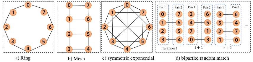
Figure 7: Different topologies with 8 nodes.

References

- [1] BlueFog: A High-performance Decentralized Training Framework for Deep Learning. https://github.com/Bluefog-Lib/bluefog.
- [2] Dan Alistarh, Demjan Grubic, Jerry Li, Ryota Tomioka, and Milan Vojnovic. Qsgd: Communication-efficient sgd via gradient quantization and encoding. In Advances in Neural Information Processing Systems, pages 1709–1720, 2017.
- [3] Mahmoud Assran, Nicolas Loizou, Nicolas Ballas, and Mike Rabbat. Stochastic gradient push for distributed deep learning. In International Conference on Machine Learning (ICML), pages 344–353, 2019.
- [4] Aditya Balu, Zhanhong Jiang, Sin Yong Tan, Chinmay Hedge, Young M Lee, and Soumik Sarkar. Decentralized deep learning using momentum-accelerated consensus. arXiv preprint arXiv:2010.11166, 2020.
- [5] Jeremy Bernstein, Jiawei Zhao, Kamyar Azizzadenesheli, and Anima Anandkumar. signsgd with majority vote is communication efficient and fault tolerant. arXiv preprint arXiv:1810.05291, 2018.
- [6] Jianshu Chen and Ali H Sayed. Diffusion adaptation strategies for distributed optimization and learning over networks. IEEE Transactions on Signal Processing, 60(8):4289–4305, 2012.
- [7] Kai Chen, Jiaqi Wang, Jiangmiao Pang, Yuhang Cao, Yu Xiong, Xiaoxiao Li, Shuyang Sun, Wansen Feng, Ziwei Liu, Jiarui Xu, et al. Mmdetection: Open mmlab detection toolbox and benchmark. arXiv preprint arXiv:1906.07155, 2019.
- [8] Tianyi Chen, Georgios Giannakis, Tao Sun, and Wotao Yin. LAG: Lazily aggregated gradient for communication-efficient distributed learning. In Advances in Neural Information Processing Systems, pages 5050–5060, 2018.
- [9] Ekin D Cubuk, Barret Zoph, Dandelion Mane, Vijay Vasudevan, and Quoc V Le. Autoaugment: Learning augmentation policies from data. arXiv preprint arXiv:1805.09501, 2018.
- [10] Jia Deng, Wei Dong, Richard Socher, Li-Jia Li, Kai Li, and Li Fei-Fei. Imagenet: A large-scale hierarchical image database. In IEEE Conference on Computer Vision and Pattern Recognition (CVPR), pages 248–255. Ieee, 2009.
- [11] John C Duchi, Alekh Agarwal, and Martin J Wainwright. Dual averaging for distributed optimization: Convergence analysis and network scaling. IEEE Transactions on Automatic control, 57(3):592–606, 2011.
- [12] Mark Everingham, Luc Van Gool, Christopher KI Williams, John Winn, and Andrew Zisserman. The pascal visual object classes (voc) challenge. International journal of computer vision, 88(2):303–338, 2010.
- [13] Hongchang Gao and Heng Huang. Periodic stochastic gradient descent with momentum for decentralized training. arXiv preprint arXiv:2008.10435, 2020.
- [14] Igor Gitman, Hunter Lang, Pengchuan Zhang, and Lin Xiao. Understanding the role of momentum in stochastic gradient methods. arXiv preprint arXiv:1910.13962, 2019.
- [15] Priya Goyal, Piotr Dollár, Ross Girshick, Pieter Noordhuis, Lukasz Wesolowski, Aapo Kyrola, Andrew Tulloch, Yangqing Jia, and Kaiming He. Accurate, large minibatch sgd: Training imagenet in 1 hour. arXiv preprint arXiv:1706.02677, 2017.
- [16] Kaiming He, Xiangyu Zhang, Shaoqing Ren, and Jian Sun. Deep residual learning for image recognition. In IEEE Conference on Computer Vision and Pattern Recognition (CVPR), pages 770–778, 2016.
- [17] Diederik P Kingma and Jimmy Ba. Adam: A method for stochastic optimization. arXiv preprint arXiv:1412.6980, 2014.
- [18] Anastasia Koloskova, Tao Lin, Sebastian U Stich, and Martin Jaggi. Decentralized deep learning with arbitrary communication compression. In International Conference on Learning Representations, 2019.
- [19] Anastasia Koloskova, Nicolas Loizou, Sadra Boreiri, Martin Jaggi, and Sebastian U Stich. A unified theory of decentralized sgd with changing topology and local updates. In International Conference on Machine Learning (ICML), pages 1–12, 2020.
- [20] Anastasia Koloskova, Sebastian Stich, and Martin Jaggi. Decentralized stochastic optimization and gossip algorithms with compressed communication. In International Conference on Machine Learning, pages 3478–3487, 2019.
- [21] Lingjing Kong, Tao Lin, Anastasia Koloskova, Martin Jaggi, and Sebastian U Stich. Consensus control for decentralized deep learning. arXiv preprint arXiv:2102.04828, 2021.
- [22] Mu Li, David G Andersen, Jun Woo Park, Alexander J Smola, Amr Ahmed, Vanja Josifovski, James Long, Eugene J Shekita, and Bor-Yiing Su. Scaling distributed machine learning with the parameter server. In 11th USENIX Symposium on Operating Systems Design and Implementation (OSDI 14), pages 583–598, 2014.
- [23] Z. Li, W. Shi, and M. Yan. A decentralized proximal-gradient method with network independent step-sizes and separated convergence rates. IEEE Transactions on Signal Processing, July 2019. early acces. Also available on arXiv:1704.07807.
- [24] Xiangru Lian, Ce Zhang, Huan Zhang, Cho-Jui Hsieh, Wei Zhang, and Ji Liu. Can decentralized algorithms outperform centralized algorithms? a case study for decentralized parallel stochastic gradient descent. In Advances in Neural Information Processing Systems, pages 5330–5340, 2017.
- [25] Xiangru Lian, Wei Zhang, Ce Zhang, and Ji Liu. Asynchronous decentralized parallel stochastic gradient descent. In International Conference on Machine Learning, pages 3043–3052, 2018.
- [26] Tao Lin, Sai Praneeth Karimireddy, Sebastian U Stich, and Martin Jaggi. Quasi-global momentum: Accelerating decentralized deep learning on heterogeneous data. arXiv preprint arXiv:2102.04761, 2021.
- [27] Tsung-Yi Lin, Piotr Dollár, Ross Girshick, Kaiming He, Bharath Hariharan, and Serge Belongie. Feature pyramid networks for object detection. In Proceedings of the IEEE conference on computer vision and pattern recognition, pages 2117–2125, 2017.
- [28] Tsung-Yi Lin, Priya Goyal, Ross Girshick, Kaiming He, and Piotr Dollár. Focal loss for dense object detection. In Proceedings of the IEEE international conference on computer vision, pages 2980–2988, 2017.
- [29] Tsung-Yi Lin, Michael Maire, Serge Belongie, James Hays, Pietro Perona, Deva Ramanan, Piotr Dollár, and C Lawrence Zitnick. Microsoft coco: Common objects in context. In European conference on computer vision, pages 740–755. Springer, 2014.
- [30] Yanli Liu, Yuan Gao, and Wotao Yin. An improved analysis of stochastic gradient descent with momentum. arXiv preprint arXiv:2007.07989, 2020.
- [31] Yaohua Liu, Wei Xu, Gang Wu, Zhi Tian, and Qing Ling. Communication-censored admm for decentralized consensus optimization. IEEE Transactions on Signal Processing, 67(10):2565–2579, 2019.
- [32] Nicolas Loizou and Peter Richtárik. Momentum and stochastic momentum for stochastic gradient, newton, proximal point and subspace descent methods. Computational Optimization and Applications, 77(3):653–710, 2020.
- [33] Songtao Lu, Xinwei Zhang, Haoran Sun, and Mingyi Hong. Gnsd: A gradient-tracking based nonconvex stochastic algorithm for decentralized optimization. In 2019 IEEE Data Science Workshop (DSW), pages 315–321. IEEE, 2019.
- [34] Qinyi Luo, Jiaao He, Youwei Zhuo, and Xuehai Qian. Prague: High-performance heterogeneity-aware asynchronous decentralized training. In Proceedings of the Twenty-Fifth International Conference on Architectural Support for Programming Languages and Operating Systems, pages 401–416, 2020.
- [35] Angelia Nedic and Asuman Ozdaglar. Distributed subgradient methods for multi-agent optimization. IEEE Transactions on Automatic Control, 54(1):48–61, 2009.
- [36] Adam Paszke, Sam Gross, Francisco Massa, Adam Lerer, James Bradbury, Gregory Chanan, Trevor Killeen, Zeming Lin, Natalia Gimelshein, Luca Antiga, et al. Pytorch: An imperative style, high-performance deep learning library. In Advances in Neural Information Processing Systems (NeurIPS), pages 8024–8035, 2019.
- [37] Pitch Patarasuk and Xin Yuan. Bandwidth optimal all-reduce algorithms for clusters of workstations. Journal of Parallel and Distributed Computing, 69(2):117–124, 2009.
- [38] Sashank J Reddi, Satyen Kale, and Sanjiv Kumar. On the convergence of adam and beyond. arXiv preprint arXiv:1904.09237, 2019.
- [39] Shaoqing Ren, Kaiming He, Ross Girshick, and Jian Sun. Faster r-cnn: towards real-time object detection with region proposal networks. IEEE transactions on pattern analysis and machine intelligence, 39(6):1137–1149, 2016.
- [40] Mark Sandler, Andrew Howard, Menglong Zhu, Andrey Zhmoginov, and Liang-Chieh Chen. Mobilenetv2: Inverted residuals and linear bottlenecks. In Proceedings of the IEEE conference on computer vision and pattern recognition, pages 4510–4520, 2018.
- [41] Ali H Sayed. Adaptation, learning, and optimization over networks. Foundations and Trends in Machine Learning, 7(ARTICLE):311–801, 2014.
- [42] Othmane Sebbouh, Robert M Gower, and Aaron Defazio. On the convergence of the stochastic heavy ball method. arXiv preprint arXiv:2006.07867, 2020.
- [43] Navjot Singh, Deepesh Data, Jemin George, and Suhas Diggavi. Squarm-sgd: Communication-efficient momentum sgd for decentralized optimization. arXiv preprint arXiv:2005.07041, 2020.
- [44] Sebastian Urban Stich. Local sgd converges fast and communicates little. In International Conference on Learning Representations (ICLR), 2019.
- [45] Mingxing Tan and Quoc Le. Efficientnet: Rethinking model scaling for convolutional neural networks. In International Conference on Machine Learning, pages 6105–6114. PMLR, 2019.
- [46] Hanlin Tang, Xiangru Lian, Ming Yan, Ce Zhang, and Ji Liu. : Decentralized training over decentralized data. In International Conference on Machine Learning, pages 4848–4856, 2018.
- [47] Hanlin Tang, Chen Yu, Xiangru Lian, Tong Zhang, and Ji Liu. Doublesqueeze: Parallel stochastic gradient descent with double-pass error-compensated compression. In International Conference on Machine Learning, pages 6155–6165. PMLR, 2019.
- [48] John Tsitsiklis, Dimitri Bertsekas, and Michael Athans. Distributed asynchronous deterministic and stochastic gradient optimization algorithms. IEEE transactions on automatic control, 31(9):803–812, 1986.
- [49] Jianyu Wang, Vinayak Tantia, Nicolas Ballas, and Michael Rabbat. Slowmo: Improving communication-efficient distributed sgd with slow momentum. In International Conference on Learning Representations, 2019.
- [50] Ran Xin, Usman A Khan, and Soummya Kar. An improved convergence analysis for decentralized online stochastic non-convex optimization. arXiv preprint arXiv:2008.04195, 2020.
- [51] Yang You, Igor Gitman, and Boris Ginsburg. Large batch training of convolutional networks. arXiv preprint arXiv:1708.03888, 2017.
- [52] Yang You, Jonathan Hseu, Chris Ying, James Demmel, Kurt Keutzer, and Cho-Jui Hsieh. Large-batch training for lstm and beyond. In Proceedings of the International Conference for High Performance Computing, Networking, Storage and Analysis, pages 1–16, 2019.
- [53] Yang You, Jing Li, Sashank Reddi, Jonathan Hseu, Sanjiv Kumar, Srinadh Bhojanapalli, Xiaodan Song, James Demmel, Kurt Keutzer, and Cho-Jui Hsieh. Large batch optimization for deep learning: Training bert in 76 minutes. arXiv preprint arXiv:1904.00962, 2019.
- [54] Yang You, Zhao Zhang, Cho-Jui Hsieh, James Demmel, and Kurt Keutzer. Imagenet training in minutes. In Proceedings of the 47th International Conference on Parallel Processing, pages 1–10, 2018.
- [55] Hao Yu, Rong Jin, and Sen Yang. On the linear speedup analysis of communication efficient momentum sgd for distributed non-convex optimization. In International Conference on Machine Learning, pages 7184–7193. PMLR, 2019.
- [56] Kun Yuan, Sulaiman A Alghunaim, Bicheng Ying, and Ali H Sayed. On the influence of bias-correction on distributed stochastic optimization. IEEE Transactions on Signal Processing, 2020.
- [57] Kun Yuan, Qing Ling, and Wotao Yin. On the convergence of decentralized gradient descent. SIAM Journal on Optimization, 26(3):1835–1854, 2016.
- [58] Kun Yuan, Bicheng Ying, and Ali H Sayed. On the influence of momentum acceleration on online learning. The Journal of Machine Learning Research, 17(1):6602–6667, 2016.
- [59] Kun Yuan, Bicheng Ying, Xiaochuan Zhao, and Ali H Sayed. Exact diffusion for distributed optimization and learning—part ii: Convergence analysis. IEEE Transactions on Signal Processing, 67(3):724–739, 2018.