On the stability of deep convolutional neural networks under irregular or random deformations

Abstract.

The problem of robustness under location deformations for deep convolutional neural networks (DCNNs) is of great theoretical and practical interest. This issue has been studied in pioneering works, especially for scattering-type architectures, for deformation vector fields $\tau(x)$ with some regularity - at least $C^{1}$. Here we address this issue for any field $\tau\in L^{\infty}(\mathbb{R}^{d};\mathbb{R}^{d})$, without any additional regularity assumption, hence including the case of wild irregular deformations such as a noise on the pixel location of an image. We prove that for signals in multiresolution approximation spaces $U_{s}$ at scale $s$, whenever the network is Lipschitz continuous (regardless of its architecture), stability in $L^{2}$ holds in the regime $\|\tau\|_{L^{\infty}}/s\ll 1$, essentially as a consequence of the uncertainty principle. When $\|\tau\|_{L^{\infty}}/s\gg 1$ instability can occur even for well-structured DCNNs such as the wavelet scattering networks, and we provide a sharp upper bound for the asymptotic growth rate. The stability results are then extended to signals in the Besov space $B^{d/2}_{2,1}$ tailored to the given multiresolution approximation. We also consider the case of more general time-frequency deformations. Finally, we provide stochastic versions of the aforementioned results, namely we study the issue of stability in mean when $\tau(x)$ is modeled as a random field (not bounded, in general) with $|\tau(x)|$, $x\in\mathbb{R}^{d}$, identically distributed variables.

1. Introduction

1.1. The problem of robustness to deformations

Broadly speaking, the last decade was certainly marked by a striking series of successes in several feature extraction tasks (especially classification of images) enjoyed by learning models based on deep convolutional neural networks (DCNNs) [25]. In parallel with such breakthroughs, a novel research line was developed with the aim of stressing the stability of DCNNs classification outputs. It was quite astonishing to learn that even the best performing DCNNs could be effectively mislead by tailor-made adversarial examples [16, 24, 31].

Let us briefly illustrate this issue by considering a function $f:\mathbb{R}^{d}\to\mathbb{R}$ - for the sake of concreteness, for $d=2$ it may be interpreted as a model of a grayscale image. The most popular ways to build an adversarial example $\tilde{f}$ involve intensity perturbations - that is $\tilde{f}(x)=f(x)+h(x)$ for some $h:\mathbb{R}^{d}\to\mathbb{R}$ - or deformations, namely $\tilde{f}(x)=F_{\tau}f(x)\coloneqq f(x-\tau(x))$ for some vector field $\tau:\mathbb{R}^{d}\to\mathbb{R}^{d}$, including natural transformations such as translations or rotations. If $\Phi$ is a classifier such that $f$ is correctly labelled, the adversarial parameters $h$ and $\tau$ are designed in such a way that $\tilde{f}$ and $f$ are sufficiently close with respect to some perceptual similarity metric, but $\Phi(\tilde{f})\neq\Phi(f)$. To be more precise, the size of the adversarial distortion is usually measured in terms of some $L^{p}$ norm of $h$ or $\tau$. We emphasize that small-in-norm deformations may result in adversarial examples which are imperceptible to the human eye, even when $\|f-\tilde{f}\|_{L^{\infty}}$ is large. It is clear that such vulnerability issues raise doubts on networks’ generalization abilities, as well as concerns on the applications of deep learning models to sensitive real-life contexts (cf. e.g. [21, 26] and the references therein).

Several adversarial attack algorithms as well as defense strategies have been designed so far (for instance, see respectively [1, 4] on one side and [9, 27] on the other one; see also the recent reviews [3, 30, 35]). At the same time, the limited scope of empirical approaches and the quest for rigorous stability guarantees motivated a deeper mathematical analysis of DCNNs. The present note precisely fits into the latter line of research, which was initiated by Mallat with pioneering contributions on wavelet-based scattering networks for the purposes of feature extraction [28]; see also [8]. Mallat’s theory has been subsequently generalized by Bölcskei and Wiatowski [33, 34] (cf. Section 2). The framework of generalized scattering networks represents a reference for our following analysis, since it does provide a testing ground and a source of inspiration for phenomena that could occur when dealing with less interpretable (e.g., trained) networks.

Regardless of the variety of the architectures, the DCNNs under our attention can be represented by a map $\Phi$ from $L^{2}(\mathbb{R}^{d})$ to some Banach space with norm ${|\kern-1.07639pt|\kern-1.07639pt|\cdot|\kern-1.07639pt|\kern-1.07639pt|}$. Stability is clearly a desirable property - for classification purposes, think for instance of different writing styles when dealing with handwritten digit recognition. As a general rule, a small distortion of $f$ into $\tilde{f}$ should correspond to small ${|\kern-1.07639pt|\kern-1.07639pt|\Phi(\tilde{f})-\Phi(f)|\kern-1.07639pt|\kern-1.07639pt|}$. In fact, it turns out that for several classes of DCNNs one can prove or at least observe empirically that $\Phi$ enjoys a Lipschitz condition:

(1.1) $${|\kern-1.07639pt|\kern-1.07639pt|\Phi(\tilde{f})-\Phi(f)|\kern-1.07639pt|\kern-1.07639pt|}\leq C\|\tilde{f}-f\|_{L^{2}},\quad f,\tilde{f}\in L^{2}(\mathbb{R}^{d}).$$

The smallest constant $C>0$ for which such an estimate holds will be denoted by ${\rm Lip}(\Phi)$. The search for approximate values of ${\rm Lip}(\Phi)$ (or at least upper bounds) is a problem of current interest, while a thorough analysis of Lipschitz regularity of neural networks remains an open problem in general. For what concerns the wavelet scattering transform, a major result in this connection was first proved by Mallat in [28], alongside with asymptotic translation invariance of the feature extractor $\Phi$; these results were extended to more general scattering networks in [33] and [5, 36]. It should be emphasized that the above Lipschitz property is also important with regard to resistance against adversarial deformations; for instance, large Lipschitz bounds have been found to be related to increased vulnerability to adversarial attacks [31]; see also [5, 36] for further details on the problem.

In the particular case of a deformation $\tilde{f}=F_{\tau}f$ of $f$, it would be desirable for ${|\kern-1.07639pt|\kern-1.07639pt|\Phi(F_{\tau}f)-\Phi(f)|\kern-1.07639pt|\kern-1.07639pt|}$ to be small whenever $\tau$ is small with respect to some metric. In this connection, for a scattering network with wavelets filters, modulus nonlinearity and no pooling, it was proved in [28, Theorem 2.12] that, for every $\tau\in C^{2}(\mathbb{R}^{d};\mathbb{R}^{d})$ with $\|\nabla\tau\|_{L^{\infty}}\leq 1/2$,

(1.2) $${|\kern-1.07639pt|\kern-1.07639pt|\Phi(F_{\tau}f)-\Phi(f)|\kern-1.07639pt|\kern-1.07639pt|}\leq C(2^{-J}\|\tau\|_{L^{\infty}}+\max\{J,1\}\|\nabla\tau\|_{L^{\infty}}+\|H\tau\|_{L^{\infty}})\|f\|_{\mathrm{scatt}}$$

where $\|f\|_{\mathrm{scatt}}$ is a mixed $\ell^{1}(L^{2})$ scattering norm (which is finite for functions with a logarithmic Sobolev-type regularity), $H\tau$ denotes the Hessian of $\tau$ and $2^{J}$ is the coarsest scale in the dyadic subband decomposition.

Some remarks are in order here. First, this estimate implies stability under (small) $C^{2}$ deformations as well as approximate invariance to global translations, up to the scale $2^{J}$. Moreover, in general we will have ${|\kern-1.07639pt|\kern-1.07639pt|\Phi(F_{\tau}f)-\Phi(f)|\kern-1.07639pt|\kern-1.07639pt|}\ll\|F_{\tau}f-f\|_{L^{2}}$ even for small $\|\tau\|_{L^{\infty}}$. Secondly, the regularity of the deformation $\tau$ plays a key role. To be clearer, consider the case where $f$ is a band-pass function; roughly speaking, the condition $\|\nabla\tau\|_{L^{\infty}}\leq 1/2$ guarantees that $F_{\tau}f$ is still localized in frequency, essentially in the same band, therefore the result is reasonable since the network is adjusted to such dyadic bands by design - although highly not-trivial to prove. As observed in [28], the condition $\|\nabla\tau\|_{L^{\infty}}\leq 1/2$ can be relaxed to $\|\nabla\tau\|_{L^{\infty}}<1$ but then the constant will blow-up when $\|\nabla\tau\|_{L^{\infty}}\to 1$. It is thus natural to wonder whether stability results can be derived if $\|\nabla\tau\|_{L^{\infty}}\geq 1$ (therefore $x\mapsto x-\tau(x)$ is no longer invertible, in general) or even for less regular deformations, e.g. discontinuous ones.

1.2. More general deformations for Lipschitz DCNNs

In this note we address the problem of DCNNs robustness in a quite general setting, precisely we consider:

• general distortions encoded by $\tau\in L^{\infty}(\mathbb{R}^{d};\mathbb{R}^{d})$ without any additional regularity assumption, therefore including wild irregular deformations such as a noise on the pixel location of an image;

• general DCNNs that are only assumed to satisfy a Lipschitz property as in (1.1) - this encompasses the case of possibly trained or unstructured filters.

These two conditions are strictly related: it turns out that for irregular deformations $\tau(x)$, even for well structured DCNNs $\Phi$ such as the wavelet scattering networks, it may happen that ${|\kern-1.07639pt|\kern-1.07639pt|\Phi(F_{\tau}f)-\Phi(f)|\kern-1.07639pt|\kern-1.07639pt|}\approx\|F_{\tau}f-f\|_{L^{2}}$ (see Section 8). Hence, the analysis should ultimately rely on estimates of the $L^{2}$ error $\|F_{\tau}f-f\|_{L^{2}}$, which in turn imply corresponding results for any Lipschitz map $\Phi$. This approach was referred to as decoupling method in [33], where bounds for $\|F_{\tau}f-f\|_{L^{2}}$ were called sensitivity estimates.

There are basically two types of peculiar phenomena that could occur when dealing with irregular deformations.

1. Consider a band-pass function $f$ oscillating at frequency $1/s$ ($s>0$ being the scale); even if $\|\tau\|_{L^{\infty}}$ is small, it may very well happen that the energy of $F_{\tau}f$ is amplified by a factor $(\|\tau\|_{L^{\infty}}/s)^{d/2}$; see Figure 1A. Hence, if $\Phi$ is any energy preserving map ($\|f\|_{L^{2}}\lesssim{|\kern-1.07639pt|\kern-1.07639pt|\Phi(f)|\kern-1.07639pt|\kern-1.07639pt|}\lesssim\|f\|_{L^{2}}$) then it follows from the triangle inequality that ${|\kern-1.07639pt|\kern-1.07639pt|\Phi(F_{\tau}f)-\Phi(f)|\kern-1.07639pt|\kern-1.07639pt|}/\|f\|_{L^{2}}\gtrsim(\|\tau\|_{L^{\infty}}/s)^{d/2}$ when $\|\tau\|_{L^{\infty}}$ is large compared to $s$.

2. Let $f$ be a band-pass function, as above, oscillating at frequency $1/s$; even if $\|\tau\|_{L^{\infty}}$ is small, when $\|\tau\|_{L^{\infty}}$ is comparable to $s$ it may happen that $f$ and $F_{\tau}f$ are localized in different dyadic frequency bands; see Figure 1B. In particular, if $\Phi$ is a wavelet scattering network, their energy will propagate along different paths and the error ${|\kern-1.07639pt|\kern-1.07639pt|\Phi(F_{\tau}f)-\Phi(f)|\kern-1.07639pt|\kern-1.07639pt|}^{2}\approx{|\kern-1.07639pt|\kern-1.07639pt|\Phi(F_{\tau}f)|\kern-1.07639pt|\kern-1.07639pt|}^{2}+{|\kern-1.07639pt|\kern-1.07639pt|\Phi(f)|\kern-1.07639pt|\kern-1.07639pt|}^{2}$ will not be small if $\Phi$ is energy preserving.

A

B

Figure 1. (A) A signal $f$ supported on $[-s,s]$ and its deformation $F_{\tau}f$, where $\tau(x)=x$ for $|x|<K$, with $K>s$. The plateau level corresponds to the value $f(0)$. The operator $F_{\tau}$ (with the choice of $\tau$ specified above) performs a single-point sampling of $f$, hence it does not make sense on discontinuous signals.
(B) A signal $f$ localized in frequency where $|\omega|\approx s^{-1}$. With the choice of the deformation $\tau=s\mathbbm{1}_{\{f=-1\}}$, the signal $F_{\tau}f$ is low-pass (a similar example with $f$ continuous is easily obtained by smoothing the steps).

These phenomena are evident sources of instability in the case where $\|\tau\|_{L^{\infty}}/s\gg 1$ and $\|\tau\|_{L^{\infty}}/s\approx 1$ respectively. Furthermore, in order for $F_{\tau}f$ to be well defined as an element of $L^{2}(\mathbb{R}^{d})$ for every $\tau\in L^{\infty}(\mathbb{R}^{d};\mathbb{R}^{d})$, independently of the representative of $f$ in $L^{2}(\mathbb{R}^{d})$ (which is only defined up to measure zero sets), $f$ must be assumed continuous at least (see again Figure 1A for a concrete example).

The previous remarks motivate recourse to multiresolution approximation spaces $U_{s}\subset L^{2}(\mathbb{R}^{d})$, $s>0$ [29], with a Riesz basis given by a sequence of functions of the type $\phi_{s,n}(x)\coloneqq s^{-d/2}\phi((x-ns)/s)$, $n\in\mathbb{Z}^{d}$, where $\phi$ is a fixed filter satisfying certain mild regularity and decay conditions (cf. Assumptions A, B and C in Section 5 below). Different choices of $\phi$ result in diverse multiresolution approximations, including band-limited functions and polynomial splines of order $n\geq 1$ - see the discussion in Example 5.1 below for more details. In general, the introduction of a fixed resolution scale is also natural as a mathematical model of a concrete signal capture system (cf. the general A/D and D/A conversion schemes in [29, Section 3.1.3] and also [6, 7] for a similar limited-resolution assumption in a discrete setting). The scale $s$ (or rather $s^{-1}$) can also be viewed as a rough measure of the complexity of the input signal, and the previous discussion suggests that the stability bounds should involve the ratio $\|\tau\|_{L^{\infty}}/s$ rather than just $\|\tau\|_{L^{\infty}}$, which is also expected in order to have dimensionally consistent estimates.

1.3. Discussion of the main results

The core of our first result can be presented as follows: under suitable assumptions on $\phi$ there exists a constant $C>0$ such that, for every $\tau\in L^{\infty}(\mathbb{R}^{d};\mathbb{R}^{d})$, $s>0$,

(1.3) $${|\kern-1.07639pt|\kern-1.07639pt|\Phi(F_{\tau}f)-\Phi(f)|\kern-1.07639pt|\kern-1.07639pt|}\leq\begin{cases}C{\rm Lip}(\Phi)(\|\tau\|_{L^{\infty}}/s)\|f\|_{L^{2}}&(\|\tau\|_{L^{\infty}}/s\leq 1)\\ C{\rm Lip}(\Phi)(\|\tau\|_{L^{\infty}}/s)^{d/2}\|f\|_{L^{2}}&(\|\tau\|_{L^{\infty}}/s\geq 1)\end{cases},\quad f\in U_{s}.$$

Here $\Phi$ is any Lipschitz map. We refer to Theorems 5.7 and 5.8 for precise statements. In short, whenever we have a Lipschitz bound, we have a stability result in the regime $\|\tau\|_{L^{\infty}}/s\ll 1$, which can be explained in heuristic terms as one of the manifold forms of the uncertainty principle. Observe also that the rate of instability agrees with that of the previous discussion in (a) when small-size oscillations, compared with the size of the deformation (namely, if $\|\tau\|_{L^{\infty}}/s\gg 1$), are allowed.

Interestingly, for fixed $f$, we have in any case ${|\kern-1.07639pt|\kern-1.07639pt|\Phi(F_{\tau}f)-\Phi(f)|\kern-1.07639pt|\kern-1.07639pt|}=O(\|\tau\|_{L^{\infty}})$ as $\|\tau\|_{L^{\infty}}\to 0$, although this asymptotic estimate is not uniform with respect to $s$. In fact, in sharp contrast with (1.2), the factor $1/s$ in front of $\|\tau\|_{L^{\infty}}$ identifies the resolution of $f$, whereas the invariance resolution $2^{-J}$ in (1.2) is a fixed parameter of the network. However, the example in item (b) above shows that in the framework of irregular deformations, even for a fixed wavelet scattering network, we cannot hope for an estimate whose quality does not deteriorate when $\|\tau\|_{L^{\infty}}$ becomes comparable to the size of the oscillations of $f$. In fact, in Section 8 we show the sharpness of the estimate (1.3) in both regimes $\|\tau\|_{L^{\infty}}/s\gg 1$ and $\|\tau\|_{L^{\infty}}/s\ll 1$ for wavelet scattering networks. We thus conclude that whereas the choice of wavelet filters is crucial in [28] to construct a transform which is Lipschitz stable to the action of $C^{2}$ diffeomorphisms, robustness under small and irregular deformations obeys a more general rule, as already anticipated above.

We remark that estimates similar to (1.3) for generalized scattering networks were proved in [33] (see also [5]) for band-limited functions and in [23] for functions in the Sobolev space $H^{1}(\mathbb{R}^{d})$ (see also [20] for other relevant signal classes, such as cartoon functions or Lipschitz functions). However, all these stability bounds for $\Phi$ are derived under the condition $\tau\in C^{1}(\mathbb{R}^{d};\mathbb{R}^{d})$, with $\|\nabla\tau\|_{L^{\infty}}$ small enough (again one could assume $\|\nabla\tau\|_{L^{\infty}}<1$ at the price of a blow-up when $\|\nabla\tau\|_{L^{\infty}}\to 1$). The estimate (1.3) for $\|\tau\|_{L^{\infty}}/s\leq 1$ thus recovers and extends the results proved in [33] for band-limited functions, now without any regularity assumption on the deformation.

The assumption that the input signal $f$ belongs to $U_{s}$ could be not realistic in practice; rather, we often deal with signals that can be well approximated in low-complexity spaces. For such signal classes we have again a stability result, which is briefly outlined here in low-dimensional settings for simplicity - we refer to Theorem 5.10 for a general and precise statement. Let $V_{j}\coloneqq U_{2^{j}}$, $j\in\mathbb{Z}$, be a multiresolution approximation of $L^{2}(\mathbb{R}^{d})$. There exists a constant $C>0$ such that, for every $\tau\in L^{\infty}(\mathbb{R}^{d};\mathbb{R}^{d})$ and any Lipschitz map $\Phi$

$${|\kern-1.07639pt|\kern-1.07639pt|\Phi(F_{\tau}f)-\Phi(f)|\kern-1.07639pt|\kern-1.07639pt|}\leq C\,{\rm Lip}(\Phi)\|\tau\|_{L^{\infty}}^{d/2}\|f\|_{\dot{B}^{d/2}_{2,1}}\qquad d=1,2$$

if $f\in L^{2}(\mathbb{R}^{d})$ and $\|f\|_{\dot{B}^{d/2}_{2,1}}<\infty$, where $\dot{B}^{d/2}_{2,1}$ denotes the homogeneous Besov space tailored to the given multiresolution approximation [29, Section 9.2.3]. This regularity level looks optimal in general: as already observed, $f$ should be at least continuous, and therefore in $B^{d/2}_{2,1}(\mathbb{R}^{d})$ if we consider the scale of $L^{2}$-based Besov spaces as a reference.

In Section 6 we prove estimates in the same spirit for more general time-frequency deformations of the type $F_{\tau,\omega}f(x)=e^{i\omega(x)}f(x-\tau(x))$. Modulation deformations are relevant in case of spectral distortions of input signals. Differently from [33], these deformations are approached here in a “perturbative” way - that is, by reducing to the results already proved for the case $\omega\equiv 0$. Moreover, in Section 7 we present a general discussion on the dimensional consistency of the above estimates for generalized scattering networks.

The main technical tools behind our results are the properties of certain spaces $X^{p,q}_{r}$, tailored to the deformation scale $r>0$. Such function spaces are usually referred to as Wiener amalgam spaces and were introduced by Feichtinger in the ’80s [13, 14]; as the name suggests, they are obtained by means of a norm that amalgamates a local summability of $L^{p}$ type on balls of radius $r$ with an $L^{q}$ behaviour at infinity. They are currently used in harmonic analysis and PDEs, possibly under slightly different names and forms; see for instance [11, 32].

In Section 3 we collect the main properties of these spaces, while in Section 4 we focus on the space $X^{\infty,2}_{r}$ of locally bounded functions, uniformly at the scale $r$, with $L^{2}$ decay. This choice should not be intended as a mere technical workaround: in Proposition 4.1 we prove indeed that this class is the optimal choice when dealing with arbitrary bounded deformations, since for functions $f\in X^{\infty,2}_{r}\cap C(\mathbb{R}^{d})$ we have the clear-cut characterization

$$\|f\|_{X^{\infty,2}_{r}}=\max\{\|F_{\tau}f\|_{L^{2}}:\tau\in L^{\infty}(\mathbb{R}^{d};\mathbb{R}^{d}),\,\|\tau\|_{L^{\infty}}\leq r\}.$$

Moreover, the local control offered by $X^{p,q}_{r}$ can be effectively exploited to prove a crucial embedding, cf. Theorem 5.3, which can be heuristically referred to as a reverse Hölder-type inequality for signals in $U_{s}$ - in the spirit of [32, Lemma 2.2] - and can be regarded as a novel form of the already mentioned uncertainty principle.

We adopted so far a deterministic model for the deformation - in fact, a ball in $L^{\infty}(\mathbb{R}^{d};\mathbb{R}^{d})$ - without any additional structure, and therefore we provided stability guarantees for the “worst-case scenario”. In Section 9 we assume instead that $\tau$ is a random field with identically distributed variables $|\tau(x)|$, $x\in\mathbb{R}^{d}$. We accordingly study the issue of stability in mean, providing stochastic versions of the above results. For example, we prove that

$$\mathbb{E}{|\kern-1.07639pt|\kern-1.07639pt|\Phi(F_{\tau}f)-\Phi(f)|\kern-1.07639pt|\kern-1.07639pt|}^{2}\leq C\,{\rm Lip}(\Phi)^{2}\mathbb{E}[|\tau|^{d}]\|f\|^{2}_{\dot{B}^{d/2}_{2,1}}\qquad d=1,2;$$

see Theorem 9.1 for the precise statement in any dimension, and for similar results when $f$ belongs to limited-resolution spaces $U_{s}$ as above. Here we set $\mathbb{E}[|\tau|^{d}]$ for $\mathbb{E}[|\tau(x)|^{d}]$, the latter being in fact independent of $x$; we also emphasize that the field $\tau$ is no longer assumed to be bounded.

To conclude, in Section 10 we briefly report on numerical evidences for scattering architectures in dimension $d=1$. We also suggest an empirical procedure aimed at the estimate of the scale parameter $s$ for certain toy signals. A more systematic experimental analysis of the problem is postponed to future work.

2. General notation and review of scattering networks

2.1. Notation

The open unit ball of $\mathbb{R}^{d}$ with radius $r>0$ and centered at the origin is denoted by $B_{r}$.

We introduce a number of operators acting on $f:\mathbb{R}^{d}\to\mathbb{C}$:

• the dilation $D_{\lambda}$ by $\lambda\neq 0$: $D_{\lambda}f(y)=f(\lambda y)$;

• the translation $T_{x}$ by $x\in\mathbb{R}^{d}$: $T_{x}f(y)=f(y-x)$;

• the modulation $M_{\xi}$ by $\xi\in\mathbb{R}^{d}$: $M_{\xi}f(y)=e^{iy\cdot\xi}f(y)$;

• the reflection: $\mathcal{I}f(y)=f(-y)$;

• the Fourier transform (whenever meaningful, e.g. if $f\in L^{1}(\mathbb{R}^{d})$), normalized here as

  $$\widehat{f}(\omega)=\mathcal{F}(f)(\omega)=\int_{\mathbb{R}^{d}}e^{-i\omega\cdot y}f(y)dy.$$

The space $L^{\infty}(\mathbb{R}^{d};\mathbb{R}^{d})$ contains all the measurable vector fields $\tau:\mathbb{R}^{d}\to\mathbb{R}^{d}$ such that

$$\|\tau\|_{L^{\infty}}\coloneqq\operatorname*{ess\,sup}_{y\in\mathbb{R}^{d}}|\tau(y)|<\infty.$$

We introduce the inhomogeneous magnitude $\langle y$ of $y\in\mathbb{R}^{d}$ by $\langle y\coloneqq(1+|y|^{2})^{1/2}$.

The symbol $\mathbbm{1}_{E}$ will be used to denote the characteristic function of a set $E$.

While in the statements of the results we will keep track of absolute constants in the estimates, in the proofs we will heavily make use of the symbol $X\lesssim Y$, meaning that the underlying inequality holds up to a “universal” positive constant factor, namely

$$X\lesssim Y\quad\Longrightarrow\quad\exists\,C>0\,:\,X\leq CY.$$

Moreover, $X\asymp Y$ means that $X$ and $Y$ are equivalent quantities, that is both $X\lesssim Y$ and $X\lesssim Y$ hold.

In the rest of the note all the derivatives are to be understood in the distribution sense, unless otherwise noted.

2.2. A brief review of generalized scattering networks

In this section we recollect some basic facts and results concerning the mathematical analysis of scattering networks, mainly in order to fix the notation and also to have a concrete reference model. More details can be found in [28, 33].

The typical architecture of a generalized scattering network ultimately consists of three parts: convolution with suitable filters, application of a non-linearity and finally some kind of pooling. To be more precise, the triplet $(\Psi_{n},M_{n},P_{n})$ (called module) represents the structure of the $n$-th layer of the network, where:

1. $\Psi_{n}=\{T_{b}\mathcal{I}g_{\lambda_{n}}:b\in\mathbb{R}^{d},\,\lambda_{n}\in\Lambda_{n}\}$ is a semi-discrete frame for $L^{2}(\mathbb{R}^{d})$ with atoms $g_{\lambda_{n}}\in L^{1}(\mathbb{R}^{d})\cap L^{2}(\mathbb{R}^{d})$ and countable index set $\Lambda_{n}$. This is equivalent to say that there exist constants $A_{n},B_{n}>0$ such that

   $$A_{n}\|f\|_{L^{2}}^{2}\leq\sum_{\lambda_{n}\in\Lambda_{n}}\|f*g_{\lambda_{n}}\|_{L^{2}}^{2}\leq B_{n}\|f\|_{L^{2}}^{2},\quad f\in L^{2}(\mathbb{R}^{d}).$$

2. $M_{n}:L^{2}(\mathbb{R}^{d})\to L^{2}(\mathbb{R}^{d})$ is a non-linear pointwise Lipschitz-continuous operator, with Lipschitz constant $L_{n}>0$, such that $M_{n}f=0$ if $f=0$.

3. $P_{n}:L^{2}(\mathbb{R}^{d})\to L^{2}(\mathbb{R}^{d})$ is a Lipschitz-continuous operator, with Lipschitz constant $R_{n}>0$, such that $P_{n}f=0$ if $f=0$. The associated pooling operator is defined by

   $$f\mapsto S_{n}^{d/2}D_{S_{n}}(P_{n}(f)),\quad f\in L^{2}(\mathbb{R}^{d}),$$

   where $S_{n}\geq 1$ is the pooling factor. In Section 7 we will assume that $P_{n}$ is a convolution operator or even the identity operator.

The sequence $\Omega=\{(\Psi_{n},M_{n},P_{n})\}_{n\in\mathbb{N}}$ is called module-sequence. We say that the latter is an admissible module-sequence if the following condition is satisfied:

(2.1) $$\max\{B_{n},B_{n}L_{n}^{2}R_{n}^{2}\}\leq 1,\quad\forall n\in\mathbb{N}.$$

For any $n\geq 1$ we arbitrarily single out an atom $g_{\lambda^{*}_{n}}$, $\lambda^{*}_{n}\in\Lambda_{n}$, and call it the output-generating atom $\chi_{n-1}$ of the $(n-1)$-th layer; we accordingly set $\chi_{n-1}\coloneqq g_{\lambda^{*}_{n}}$ and rename $\Lambda_{n}\setminus\{g_{\lambda^{*}_{n}}\}$ by $\Lambda_{n}$.

Given an integer $n\geq 1$ we introduce the set of $n$-paths to be $\Lambda^{n}\coloneqq\Lambda_{1}\times\cdots\times\Lambda_{n}$, while $\Lambda^{0}\coloneqq\{\emptyset\}$. The set of all possible paths is thus given by $\mathcal{Q}\coloneqq\bigcup_{n=0}^{\infty}\Lambda^{n}$.

The $n$-th layer scattering propagator $U_{n}:\Lambda_{n}\times L^{2}(\mathbb{R}^{d})\to L^{2}(\mathbb{R}^{d})$ is defined by

$$U_{n}[\lambda_{n}](f)\coloneqq S^{d/2}_{n}D_{S_{n}}P_{n}(M_{n}(f*g_{\lambda_{n}})).$$

More generally, the scattering propagator $U:\Lambda^{n}\times L^{2}(\mathbb{R}^{d})\to L^{2}(\mathbb{R}^{d})$ acts on a path $q=(\lambda_{1},\ldots,\lambda_{n})\in\Lambda^{n}$ by

$$U[q](f)\coloneqq U_{n}[\lambda_{n}]\cdots U_{2}[\lambda_{2}]U_{1}[\lambda_{1}](f)$$

and $U(\emptyset)f=f$.

treenode/.style = align=center, inner sep=0pt, text centered, font=, for tree= grow’=north, delay= edge label/.wrap value=node[midway, font=, above]#1, , [$f$, name=L0, [$U[\lambda_{1}^{(j)}]f$, name=L1sx , [ $\displaystyle U[\lambda_{1}^{(j)},\lambda_{2}^{(k)}]f$ , name=L2sx, [$\vdots$] [$\vdots$] [$\vdots$] [$\vdots$] ] [, tikz=[fill=white] (.anchor) circle[radius=2pt]; [$\vdots$] [$\vdots$] ] [, tikz=[fill=white] (.anchor) circle[radius=2pt]; [$\vdots$] [$\vdots$] ] ] [,tikz=[fill=white] (.anchor) circle[radius=2pt]; [, tikz=[fill=white] (.anchor) circle[radius=2pt]; [$\vdots$]], [, tikz=[fill=white] (.anchor) circle[radius=2pt]; [$\vdots$]]] [$U[\lambda_{1}^{(r)}]f$, name=L1dx, [, tikz=[fill=white] (.anchor) circle[radius=2pt]; [$\vdots$] ] [,tikz=[fill=white] (.anchor) circle[radius=2pt]; [$\vdots$] ] [ $\displaystyle U[\lambda_{1}^{(r)},\lambda_{2}^{(s)}]f$ , name=L2dx, [,tikz=[fill=white] (.anchor) circle[radius=2pt]; [$\vdots$][$\vdots$][$\vdots$] ] [$\cdots$, [ $\displaystyle U[\lambda_{1}^{(r)},\lambda_{2}^{(s)},\ldots,\lambda_{n}^{(t)}]f$ , name=Ldxend, [$\vdots$,for ancestors=edge=red,thick] [$\vdots$] [$\vdots$]] ] ] ] ] ] [blue, dashed, -¿, shorten ¿=3pt] (L0) – ++(-27pt,-20pt) node [circle,fill=blue,inner sep=1pt,minimum size=3pt,label=[xshift=0pt, yshift=-15pt] $\displaystyle f*\chi_{0}$ ] ;; [blue, dashed, dashed, -¿, shorten ¿=3pt] (L1sx) – ++(-40pt,-30pt) node [circle,fill=blue,inner sep=1pt,minimum size=3pt,label=[xshift=0pt,yshift=-20pt] $\displaystyle(U[\lambda_{1}^{(j)}]f)*\chi_{1}$ ] ;; [blue, dashed, -¿, shorten ¿=3pt] (L2sx) – ++(-40pt,-30pt) node [circle,fill=blue,inner sep=1pt,minimum size=3pt,label=[xshift=0pt,yshift=-20pt] $\displaystyle(U[\lambda_{1}^{(j)}\lambda_{2}^{(k)}]f)*\chi_{2}$ ] ;; [blue, dashed, -¿, shorten ¿=3pt] (L1dx) – ++(50pt,-25pt) node [circle,fill=blue,inner sep=1pt,minimum size=3pt,label=[xshift=0pt,yshift=-20pt] $\displaystyle(U[\lambda_{1}^{(r)}]f)*\chi_{1}$ ] ;; [blue, dashed, -¿, shorten ¿=3pt] (L2dx) – ++(50pt,-25pt) node [circle,fill=blue,inner sep=1pt,minimum size=3pt,label=[xshift=0pt,yshift=-20pt] $\displaystyle(U[\lambda_{1}^{(r)},\lambda_{2}^{(s)}]f)*\chi_{2}$ ] ;; [blue, dashed, -¿, shorten ¿=3pt] (Ldxend) – ++(50pt,-25pt) node [circle,fill=blue,inner sep=1pt,minimum size=3pt,label=[xshift=0pt,yshift=-20pt] $\displaystyle(U[\lambda_{1}^{(r)},\lambda_{2}^{(s)},\ldots,\lambda_{n}^{(t)}]f)*\chi_{n}$ ] ;;

Figure 2. A typical scattering network architecture, as described above. The index $\lambda_{l}^{(m)}$ corresponds to the $m$-th atom of the $l$-th layer frame $\Phi_{l}$. In blue: some features, where $\chi_{l}$ is the output-generating atom of the $l$-th layer. In red: an example of a $n$-path $q=(\lambda_{1}^{(r)},\lambda_{2}^{(s)}\ldots,\lambda_{n}^{(t)})\in\Lambda^{n}$.

Given an admissible module-sequence $\Omega=\{(\Psi_{n},M_{n},P_{n})\}_{n\in\mathbb{N}}$ the feature extractor $\Phi_{\Omega}:L^{2}(\mathbb{R}^{d})\to\ell^{2}(\mathcal{Q};L^{2}(\mathbb{R}^{d}))$ is defined by

$$\Phi_{\Omega}(f)\coloneqq\left\{\Phi_{\Omega}^{n}(f)\right\}_{n\geq 0},\quad\Phi_{\Omega}^{n}(f)\coloneqq\{(U[q](f))*\chi_{n}:q\in\Lambda^{n}\},$$

where $\ell^{2}(\mathcal{Q};L^{2}(\mathbb{R}^{d}))$ consists of all the sequences of the form $s=\{s_{q}\in L^{2}(\mathbb{R}^{d}):q\in\mathcal{Q}\}$ such that

$${|\kern-1.07639pt|\kern-1.07639pt|s|\kern-1.07639pt|\kern-1.07639pt|}\coloneqq\left(\sum_{q\in\mathcal{Q}}\|s_{q}\|_{2}^{2}\right)^{1/2}<\infty.$$

The two main properties of the feature extractor are recalled below.

Vertical invariance [33, Theorem 1]. If

$$M_{n}(T_{c}f)=T_{c}M_{n}(f),\quad P_{n}(T_{c}f)=T_{c}P_{n}(f),$$

for every $n\in\mathbb{N}$, $c\in\mathbb{R}^{d}$ and $f\in L^{2}(\mathbb{R}^{d})$, then the features $\Phi_{\Omega}^{n}(f)$ generated in the $n$-th layer satisfy

(2.2) $$\Phi_{\Omega}^{n}(T_{c}f)=\begin{cases}T_{c}\Phi_{\Omega}^{n}(f)&(n=0)\\ T_{\frac{c}{S_{1}\cdots S_{n}}}\Phi_{\Omega}^{n}(f)&(n\geq 1)\end{cases},$$

for all $f\in L^{2}(\mathbb{R}^{d})$, $c\in\mathbb{R}^{d}$ and $n\in\mathbb{N}$, where $T_{c}\Phi_{\Omega}^{n}(f)\coloneqq\{T_{c}h:h\in\Phi_{\Omega}^{n}\}$.

Lipschitz property [33, Proposition 4]. If $\Omega=\{(\Psi_{n},M_{n},P_{n})\}_{n\in\mathbb{N}}$ is an admissible module-sequence, the corresponding feature extractor $\Phi_{\Omega}:L^{2}(\mathbb{R}^{d})\to\ell^{2}(\mathcal{Q};L^{2}(\mathbb{R}^{d}))$ is Lipschitz continuous with constant ${\rm Lip}(\Phi_{\Omega})\leq 1$, that is

(2.3) $${|\kern-1.07639pt|\kern-1.07639pt|\Phi_{\Omega}(f)-\Phi_{\Omega}(h)|\kern-1.07639pt|\kern-1.07639pt|}\leq\|f-h\|_{L^{2}},\quad f,h\in L^{2}(\mathbb{R}^{d}).$$

Different sufficient conditions can be found for instance in [5, Theorem 2.1].

Interestingly, inspecting the admissibility condition (2.1) and the proofs of the previous results shows that the lower frame bounds $A_{n}$ are not involved. In fact, as remarked in [33, Section V], one could consider relaxing the assumptions on $\Psi_{n}$ in order to just deal with a semi-discrete Bessel sequence with Bessel constant $B_{n}$; see also the formulations in [5, 36] in this respect.

An important special case is represented by wavelet scattering networks, where in every layer the filters are of wavelets type, with modulus nonlinearity ($M_{n}(f)=|f|$) and no pooling ($S_{n}=1$ and $P_{n}$ is the identity operator). For example, in dimension $d=1$, Figure 4 represents the Shannon wavelet filters in the Fourier domain (we will use this architecture in a counterexample in Section 8).

3. Wiener amalgam spaces at different scales

The following family of function spaces will play a key role in the following.

Definition 3.1.

For $1\leq p,q\leq\infty$ and $r>0$, we denote by $X^{p,q}_{r}$ the space of all the complex-valued measurable functions in $\mathbb{R}^{d}$ such that

(3.1) $$\|f\|_{X^{p,q}_{r}}\coloneqq\left(\int_{\mathbb{R}^{d}}\|T_{-x}f\|_{L^{p}(B_{r})}^{q}dx\right)^{1/q}<\infty,$$

with obvious modifications if $q=\infty$. In the case where $r=1$ we write $X^{p,q}$ for $X^{p,q}_{1}$.

Let us emphasize that $X^{\infty,1}$ coincides with the well known Wiener space of harmonic analysis (cf. e.g. [18, Section 6.1]). More generally, $X^{p,q}$ coincides with the Wiener amalgam space $W(L^{p},L^{q})$ of functions with local regularity of $L^{p}$ type and global decay of $L^{q}$ type, first introduced by Feichtinger in the ’80s [13, 14]; recall that the latter is a Banach space provided with the norm

$$\|f\|_{W(L^{p},L^{q})}=\left(\int_{\mathbb{R}^{d}}\|T_{-x}f\|_{L^{p}(Q)}^{q}dx\right)^{1/p},$$

where $Q\subset\mathbb{R}^{d}$ is an arbitrary compact set with non-empty interior. In fact, different choices of $Q$ yield equivalent norms; typical choices include $Q=B_{1}$ and $Q=[0,1]^{d}$. Moreover, the following equivalent discrete-type norm can be used to measure the amalgamated regularity:

(3.2) $$\|f\|_{X^{p,q}}\asymp\left(\sum_{k\in\mathbb{Z}^{d}}\|T_{-k}f\|_{L^{p}(Q)}^{q}\right)^{1/q},\quad Q=[0,1]^{d}.$$

We also highlight that $X^{p,p}_{r}$ coincides with $L^{p}(\mathbb{R}^{d})$ as set for any $1\leq p\leq\infty$, but the norm is rescaled:

$$\|f\|_{X^{p,p}_{r}}=r^{d/p}\|f\|_{L^{p}}.$$

A similar change-of-scale property holds with respect to $X^{p,q}$, in the sense of the following result.

Lemma 3.2.

For any $1\leq p,q\leq\infty$ and $r>0$, we have that $X^{p,q}_{r}=X^{p,q}$ as sets, and

$$\|f\|_{X^{p,q}_{r}}=r^{d\left(\frac{1}{p}+\frac{1}{q}\right)}\|D_{r}f\|_{X^{p,q}}.$$

Proof.

Let us consider the case $p,q<\infty$ for conciseness, the other cases following easily. A straightforward computation shows that

$$\|f\|_{X^{p,q}_{r}} =\left(\int_{\mathbb{R}^{d}}\left(\int_{B_{r}}|f(x+y)|^{p}dy\right)^{q/p}dx\right)^{1/q}$$

$$=r^{d/p}\left(\int_{\mathbb{R}^{d}}\left(\int_{B_{1}}|f(x+rz)|^{p}dz\right)^{q/p}dx\right)^{1/q}$$

$$=r^{d/p}\left(\int_{\mathbb{R}^{d}}\left(\int_{B_{1}}|D_{r}f(r^{-1}x+z)|^{p}dz\right)^{q/p}dx\right)^{1/q}$$

$$=r^{d(1/p+1/q)}\left(\int_{\mathbb{R}^{d}}\left(\int_{B_{1}}|D_{r}f(x+z)|^{p}dz\right)^{q/p}dx\right)^{1/q},$$

that is the claim. ∎

For future reference let us examine some properties of the spaces $X^{p,q}_{r}$. First, we prove an embedding result that will be often used below.

Proposition 3.3.

For any $1\leq p_{1},p_{2},q\leq\infty$ with $p_{1}\leq p_{2}$, and $r>0$, we have

$$\|f\|_{X^{p_{1},q}_{r}}\leq Cr^{d\left(\frac{1}{p_{1}}-\frac{1}{p_{2}}\right)}\|f\|_{X^{p_{2},q}_{r}},$$

where the constant $C>0$ depends only on $d$.

Proof.

Fix $x\in\mathbb{R}^{d}$ and consider the mapping $h_{x}:y\mapsto|f(x+y)|$. The standard Hölder inequality on the ball $B_{r}$ yields, with $\rho$ such that $1/p_{1}=1/p_{2}+1/\rho$,

$$\|T_{-x}f\|_{L^{p_{1}}(B_{r})} =\|h_{x}\cdot\mathbbm{1}_{B_{r}}\|_{L^{p_{1}}(B_{r})}$$

$$\leq\|T_{-x}f\|_{L^{p_{2}}(B_{r})}\|1_{B_{r}}\|_{L^{\rho}}$$

$$\leq(Cr^{d})^{\left(\frac{1}{p_{1}}-\frac{1}{p_{2}}\right)}\|T_{-x}f\|_{L^{p_{2}}(B_{r})},$$

where $C$ is the volume of the $d$-ball with radius $1$. The claim thus follows. ∎

In the following results we illustrate the behaviour of the spaces $X^{p,q}_{r}$ under convolution and dilations. In fact, the case with $r=1$ is covered by the standard theory of amalgam spaces (cf. [13, 22] and [10, Proposition 2.2] respectively), hence the result for $r\neq 1$ follows by rescaling the norms in accordance with Lemma 3.2.

Proposition 3.4.

For any $r>0$ and $1\leq p_{1},p_{2},p,q_{1},q_{2},q\leq\infty$ such that

$$\frac{1}{p_{1}}+\frac{1}{p_{2}}=1+\frac{1}{p},\qquad\frac{1}{q_{1}}+\frac{1}{q_{2}}=1+\frac{1}{q},$$

we have

$$\|f*g\|_{X^{p,q}_{r}}\leq Cr^{-d}\|f\|_{X^{p_{1},q_{1}}_{r}}\|g\|_{X^{p_{2},q_{2}}_{r}},$$

for a constant $C>0$ that depends only on $d$.

Proposition 3.5.

For any $r,s>0$ and $1\leq p,q\leq\infty$ we have

$$\|D_{s}f\|_{X^{p,q}_{r}}\leq\begin{cases}Cs^{-d\max(1/p,1/q)}\|f\|_{X^{p,q}_{r}}&(0<s\leq 1)\\ Cs^{-d\min(1/p,1/q)}\|f\|_{X^{p,q}_{r}}&(s\geq 1)\end{cases},$$

for a constant $C>0$ that depends only on $d$.

4. $L^{\infty}$ deformations and the space $X^{\infty,2}_{r}$

Let us consider the class of deformation mappings $F_{\tau}$ associated with distortion functions $\tau:\mathbb{R}^{d}\to\mathbb{R}^{d}$ by setting

$$F_{\tau}f(x)\coloneqq f(x-\tau(x)),$$

where $f:\mathbb{R}^{d}\to\mathbb{C}$.

We prove that the class $X^{\infty,2}_{r}$ is the optimal choice as far as sensitivity bounds for arbitrary bounded deformations are concerned. The second part of the following result can be regarded as a linearization of a maximal operator (cf. [17, Section 6.1.3]).

Proposition 4.1.

We have

(4.1) $$\|F_{\tau}f\|_{L^{2}}\leq\|f\|_{X^{\infty,2}_{r}},\quad r=\|\tau\|_{L^{\infty}},$$

for every $f\in X^{\infty,2}_{r}\cap C(\mathbb{R}^{d})$ and $\tau\in L^{\infty}(\mathbb{R}^{d};\mathbb{R}^{d})$.

More precisely, for every function $f\in X^{\infty,2}_{r}\cap C(\mathbb{R}^{d})$, we have the characterization

(4.2) $$\|f\|_{X^{\infty,2}_{r}}=\max\{\|F_{\tau}f\|_{L^{2}}\,:\,\tau\in L^{\infty}(\mathbb{R}^{d};\mathbb{R}^{d}),\,\|\tau\|_{L^{\infty}}\leq r\}.$$

Remark 4.2.

Note that the continuity assumption on $f\in X^{\infty,2}_{r}$ is essential in the statement, otherwise $f(x-\tau(x))$ may not even be well defined in $L^{2}$ (i.e., independent of the representative $f$), as evidenced by the case $\tau(x)=x$ for $x\in B_{R}$ and small $R>0$. See also Figure 1A in this connection.

Proof of Proposition 4.1.

It is clear that, for almost every $x\in\mathbb{R}^{d}$,

$$|f(x-\tau(x))|\leq\sup\{|f(x-y)|:y\in\mathbb{R}^{d},\,|y|\leq\|\tau\|_{L^{\infty}}\},$$

and thus (4.1) follows after taking the $L^{2}$ norm (the above supremum is the same as the essential supremum because $f$ is continuous).

For what concerns (4.2), it is enough to prove that

$$\|f\|_{X^{\infty,2}_{r}}\leq\max\{\|F_{\tau}f\|_{L^{2}}\,:\,\tau\in L^{\infty}(\mathbb{R}^{d};\mathbb{R}^{d}),\,\|\tau\|_{L^{\infty}}\leq r\}.$$

To this aim, notice that if we could design a measurable correspondence $\tau$ between $x\in\mathbb{R}^{d}$ and a point $y^{*}=\tau(x)\in\overline{B_{r}}$ where the function $\overline{B_{r}}\ni y\mapsto|f(x-y)|$ attains its maximum, then

$$\max_{|y|\leq r}|f(x-y)|=|f(x-\tau(x))|=|F_{\tau}(x)|,$$

and the desired conclusion would follow once taking the $L^{2}$ norm. The existence of such a measurable selector is a consequence of the measurable maximum theorem [2, Theorem 18.19] (in fact, an easier argument - cf. [17, Section 6.1.3] - would give (4.2) with the supremum in place of the maximum). ∎

The following result provides a sensitivity bound for $L^{2}$ functions which are locally Lipschitz, uniformly at the deformation scale. It should be compared with the result in [23], valid for functions in the Sobolev space $H^{1}(\mathbb{R}^{d})$, for deformation $\tau\in C^{1}(\mathbb{R}^{d};\mathbb{R}^{d})$, $\|\nabla\tau\|_{L^{\infty}}\leq 1/2$, hence regular.

Proposition 4.3.

There exists a constant $C>0$ such that

(4.3) $$\|F_{\tau}f-f\|_{2}\leq C\|\tau\|_{L^{\infty}}\|\nabla f\|_{X^{\infty,2}_{r}},\quad r=\|\tau\|_{L^{\infty}},$$

for every $\tau\in L^{\infty}(\mathbb{R}^{d};\mathbb{R}^{d})$ and every function $f\in X^{\infty,2}_{r}$ such that $\|\nabla f\|_{X^{\infty,2}_{r}}<\infty$.

Observe that the condition $\|\nabla f\|_{X^{\infty,2}_{r}}<\infty$ implies that $\nabla f\in L^{\infty}_{\mathrm{loc}}(\mathbb{R}^{d})$, and therefore $f$ is locally Lipschitz continuous after possibly being redefined on a set of measure zero (cf. [12, Theorem 4, page 294]), in particular $f$ is continuous. In the following we will always identify $f$ with its continuous version. Also, we set

(4.4) $$\|\nabla f\|_{X^{\infty,2}_{r}}\coloneqq\||\nabla f|\|_{X^{\infty,2}_{r}}.$$

Proof of Proposition 4.3.

For $x\in\mathbb{R}^{d}$, $r>0$ let $B(x,r)$ be the open ball in $\mathbb{R}^{d}$ of radius $r$ and center $x$. By the Poincaré inequality for a ball (cf. [12, Theorem 2, page 291]) we see that there exists a constant $C>0$ such that, for every $r>0$ and $x\in\mathbb{R}^{d}$,

(4.5) $$|f(x-y)-f(x)|\leq Cr\|\nabla f\|_{L^{\infty}(B(x,r))},\quad|y|\leq r.$$

Setting $y=\tau(x)$, $r=\|\tau\|_{L^{\infty}}$ and taking the $L^{2}$ norm lead to the desired conclusion. ∎

5. Multiresolution approximation spaces

Fix $\phi\in L^{2}(\mathbb{R}^{d})$ and recall [29] that the associated approximation space $U_{s}$ at scale $s>0$ is defined as follows:

$$U_{s}\coloneqq\overline{\text{span}\{\phi_{s,n}\}_{n\in\mathbb{Z}^{d}}},\qquad\phi_{s,n}(x)\coloneqq s^{-d/2}T_{ns}D_{1/s}\phi(x)=s^{-d/2}\phi\left(\frac{x-ns}{s}\right).$$

In the rest of the paper we are going to deal with the following assumptions on $\phi$.

Assumption A.

There exist constants $A,B>0$ such that

(5.1) $$A\leq\sum_{k\in\mathbb{Z}^{d}}|\hat{\phi}(\omega-2\pi k)|^{2}\leq B\quad\text{for a.e. }\omega\in\mathbb{R}^{d}.$$

This is equivalent to assuming that $\{\phi_{s,n}\}$ is a Riesz basis for $U_{s}$ - see [29, Theorem 3.4] for the case $d=1$, while the result for $d>1$ is a direct extension of the latter.

We further assume one of the following regularity/decay conditions on $\phi$.

Assumption B.

At least one of the following conditions holds.

1. $\phi$ belongs to the Wiener space:

   (5.2) $$\phi\in X^{\infty,1},$$

   (in particular $\phi$ is locally bounded and has a $L^{1}$ decay);

2. There exist $\alpha>1/2$ and $B^{\prime}>0$ such that

   (5.3) $$\sum_{k\in\mathbb{Z}^{d}}|(v^{\alpha}\hat{\phi})(\omega-2\pi k)|^{2}\leq B^{\prime}\quad\text{for a.e. }\omega\in[0,2\pi],$$

   where we introduced the weight function $v(\omega)=\langle\omega_{1}\cdots\langle\omega_{d}$, $\omega\in\mathbb{R}^{d}$.

Assumption C.

For all $j=1,\ldots,d$, at least one of the conditions (5.2) and (5.3) of Assumption B is satisfied with $\phi$ replaced by $\partial_{j}\phi$.

Example 5.1.

This is a convenient stage where to present some examples of functions satisfying the assumptions. Generally speaking, (5.2) is satisfied by any function $\phi\in L^{\infty}(\mathbb{R}^{d})$ with compact support, while the same condition on the Fourier side (i.e., $\hat{\phi}\in L^{\infty}(\mathbb{R}^{d})$ with compact support) guarantees that 5.3 holds. To be more concrete, let us provide some standard examples in dimension $d=1$ - Assumption A will be satisfied in all cases (cf. [29, Section 3.1.3, pages 69,70]).

• The choice $\phi=\mathbbm{1}_{[0,1]}$, leading to piecewise constant approximations (block sampling), is easily seen to satisfy (5.2) but not (5.3) for any $\alpha>1/2$, nor Assumption C.

• The normalized sinc function $\displaystyle\phi(t)=\frac{\sin(\pi t)}{\pi t}$, corresponding to Shannon approximations (i.e., band-limited functions), satisfies (5.3) for every $\alpha>0$, as well as Assumption C, but not (5.2).

• The B-spline $\phi$ of degree $n$, obtained by $n+1$ convolutions of $\mathbbm{1}_{[0,1]}$ with itself and centering at $0$ or $1/2$, can be characterized by its Fourier transform:

  $$\hat{\phi}(\omega)=\left(\frac{\sin(\omega/2)}{\omega/2}\right)^{n+1}e^{-i\epsilon\omega/2},\quad\epsilon=\begin{cases}1&(n\text{ is even})\\ 0&(n\text{ is odd})\end{cases}.$$

  We see that if $n\geq 1$ then both (5.2) and (5.3) are satisfied (for $\alpha<n+1/2$), as well as Assumption C (the case $n=0$ is covered by the previous case of $\phi=\mathbbm{1}_{[0,1]}$).

In Assumption B we introduced the weight function $v(x)$. Let us now define a companion Sobolev space, for $\alpha\in\mathbb{R}$, $\alpha\geq 0$:

$$H^{\alpha}_{\otimes}(\mathbb{R}^{d})\coloneqq\{f\in L^{2}(\mathbb{R}^{d}):\ \|f\|_{H^{\alpha}_{\otimes}}\coloneqq\|v^{\alpha}\hat{f}\|_{L^{2}}<\infty\}.$$

Roughly speaking, $H^{\alpha}_{\otimes}(\mathbb{R}^{d})$ consists of functions in $L^{2}(\mathbb{R}^{d})$ which have at least $\alpha$ (possibly fractional) derivatives in the directions of the axes in $L^{2}(\mathbb{R}^{d})$. It is easy to realize that this space contains functions in the usual Sobolev space $H^{d\alpha}(\mathbb{R}^{d})$ as well as tensor products $\phi_{1}\otimes\ldots\otimes\phi_{d}$, with $\phi_{j}\in H^{\alpha}(\mathbb{R})$, $j=1,\ldots,d$.

Proposition 5.2.

If $\alpha>1/2$ we have the embedding $H^{\alpha}_{\otimes}(\mathbb{R}^{d})\hookrightarrow L^{\infty}(\mathbb{R}^{d})\cap C(\mathbb{R}^{d})$, as well as

$$H^{\alpha}_{\otimes}(\mathbb{R}^{d})\hookrightarrow X^{\infty,2}.$$

Proof.

The embedding in $L^{\infty}$ follows at once from the chain of inequalities

$$\|f\|_{L^{\infty}}\lesssim\|\hat{f}\|_{L^{1}}\leq\|v^{-\alpha}\|_{L^{2}}\|\hat{f}v^{\alpha}\|_{L^{2}}$$

and the fact that $v^{-\alpha}\in L^{2}(\mathbb{R}^{d})$ if $\alpha>1/2$. The embedding in $C(\mathbb{R}^{d})$ is then clear because the space of Schwartz functions is easily seen to be dense in $H^{\alpha}_{\otimes}(\mathbb{R}^{d})$.

Concerning the embedding in $X^{\infty,2}$, let $g\in C^{\infty}_{c}(\mathbb{R}^{d})$, with $g=1$ on $B_{1}$. Then

$$\|f\|_{X^{\infty,2}}\leq\|\|T_{-x}f\cdot g\|_{L^{\infty}}\|_{L^{2}_{x}}\lesssim\|\|f\cdot T_{x}g\|_{H^{\alpha}_{\otimes}}\|_{L^{2}_{x}}\lesssim\|f\|_{H^{\alpha}_{\otimes}},$$

where the last inequality is proved in [18, Propositon 11.3.1(c)]. ∎

We now establish a crucial reverse Hölder-type inequality for functions in $U_{s}$.

Theorem 5.3.

Let $\phi\in L^{2}(\mathbb{R}^{d})$ be such that Assumption A is satisfied.

1. If Assumption B holds then there exists $C>0$ such that, for every $r,s>0$,

   (5.4) $$\|f\|_{X^{\infty,2}_{r}}\leq C(1+r/s)^{d/2}\|f\|_{L^{2}},\quad f\in U_{s}.$$

2. If Assumption C holds then there exists $C>0$ such that, for every $r,s>0$,

   (5.5) $$\|\nabla f\|_{X^{\infty,2}_{r}}\leq Cs^{-1}(1+r/s)^{d/2}\|f\|_{L^{2}},\quad f\in U_{s}.$$

Remark 5.4.

Let $P_{U_{s}}$ be the orthogonal projection operator on $U_{s}$. Since $\|P_{U_{s}}\|_{L^{2}\to L^{2}}=1$, (5.4) is equivalent to

$$\|P_{U_{s}}f\|_{X^{\infty,2}_{r}}\leq C(1+r/s)^{d/2}\|f\|_{L^{2}},\quad f\in L^{2}(\mathbb{R}^{d}).$$

Proof of Theorem 5.3.

Let us commence with the proof of (5.4). Let $\{\tilde{\phi}_{s,n}\}_{n\in\mathbb{Z}^{d}}$ be the dual basis to $\{{\phi}_{s,n}\}_{n\in\mathbb{Z}^{d}}$. If $f\in U_{s}$ then

$$f=\sum_{n\in\mathbb{Z}^{d}}a_{n}\phi_{s,n},\quad a_{n}\coloneqq\langle f,\tilde{\phi}_{s,n}$$

and by Lemma 3.2 we have

$$\|f\|_{X^{\infty,2}_{r}} =r^{d/2}\|D_{r}f\|_{X^{\infty,2}}$$

$$=\left\|\sum_{n\in\mathbb{Z}^{d}}a_{n}\phi_{s/r,n}\right\|_{X^{\infty,2}}$$

$$=\left(\frac{r}{s}\right)^{d/2}\left\|\sum_{n\in\mathbb{Z}^{d}}a_{n}\phi\left(\frac{r}{s}\cdot\,-n\right)\right\|_{X^{\infty,2}}$$

$$=\left(\frac{r}{s}\right)^{d/2}\left\|\left\|\sum_{n\in\mathbb{Z}^{d}}a_{n}\phi\left(\frac{r}{s}(x+y)-n\right)\mathbbm{1}_{B_{1}}(y)\right\|_{L^{\infty}_{y}}\right\|_{L^{2}_{x}}$$

$$=\left\|\left\|\sum_{n\in\mathbb{Z}^{d}}a_{n}\phi(x+y-n)\mathbbm{1}_{B_{r/s}}(y)\right\|_{L^{\infty}_{y}}\right\|_{L^{2}_{x}}$$

$$=\left\|\sum_{n\in\mathbb{Z}^{d}}a_{n}T_{n}\phi\right\|_{X^{\infty,2}_{r/s}}$$

(5.6) $$\lesssim\left(1+\frac{r}{s}\right)^{d/2}\left\|\sum_{n\in\mathbb{Z}^{d}}a_{n}T_{n}\phi\right\|_{X^{\infty,2}},$$

where in the last step we used Lemma 3.2 and Proposition 3.5.

Assume now (5.2), namely $\phi\in X^{\infty,1}$. Then the conclusion follows from (5.6) using the equivalent discrete-type norm in (3.2) (with $Q=[0,1]^{d}$):

$$\|f\|_{X^{\infty,2}_{r}} \lesssim\left(1+\frac{r}{s}\right)^{d/2}\left\|\sum_{n\in\mathbb{Z}^{d}}a_{n}T_{n}\phi\right\|_{X^{\infty,2}}$$

$$\lesssim\left(1+\frac{r}{s}\right)^{d/2}\left\|\sum_{n\in\mathbb{Z}^{d}}|a_{n}|\|\phi(k+y-n)\mathbbm{1}_{Q}\|_{L^{\infty}_{y}}\right\|_{\ell^{2}_{k}}$$

$$\lesssim\left(1+\frac{r}{s}\right)^{d/2}\left(\sum_{k\in\mathbb{Z}^{d}}\|\phi(k+y)\mathbbm{1}_{Q}\|_{L^{\infty}_{y}}\right)\left(\sum_{n\in\mathbb{Z}^{d}}|a_{n}|^{2}\right)^{1/2}$$

$$\lesssim\left(1+\frac{r}{s}\right)^{d/2}\|\phi\|_{X^{\infty,1}}\|f\|_{L^{2}},$$

where we used that $\ell^{1}*\ell^{2}\hookrightarrow\ell^{2}$ and $\|a_{n}\|_{\ell^{2}}\lesssim\|f\|_{L^{2}}$.

Let us assume (5.3) instead. By (5.6), it is enough to show that

$$\left\|\sum_{n\in\mathbb{Z}^{d}}a_{n}T_{n}\phi\right\|_{X^{\infty,2}}\lesssim\|f\|_{L^{2}}.$$

Using the embedding in Proposition 5.2 we obtain

$$\left\|\sum_{n\in\mathbb{Z}^{d}}a_{n}T_{n}\phi\right\|_{X^{\infty,2}} \lesssim\left\|\sum_{n\in\mathbb{Z}^{d}}a_{n}T_{n}\phi\right\|_{H^{\alpha}_{\otimes}}$$

$$=\left\|\sum_{n\in\mathbb{Z}^{d}}a_{n}e^{-in\omega}\hat{\phi}(\omega)v^{\alpha}(\omega)\right\|_{L^{2}}$$

$$=\left(\int_{[0,2\pi]^{d}}\sum_{k\in\mathbb{Z}^{d}}|F(\omega)(v^{\alpha}\hat{\phi})(\omega-2\pi k)|^{2}d\omega\right)^{1/2}$$

$$\leq\|F\|_{L^{2}([0,2\pi]^{d})}\left(\operatorname*{ess\,sup}_{\omega\in[0,2\pi]}\sum_{k\in\mathbb{Z}^{d}}|(v^{\alpha}\hat{\phi})(\omega-2\pi k)|^{2}\right)^{1/2}$$

$$\lesssim\|f\|_{L^{2}},$$

where we set $F(\omega)\coloneqq\sum_{n\in\mathbb{Z}^{d}}a_{n}e^{-in\omega}$ (which is a $2\pi$-periodic, square integrable on $[0,2\pi]$, function), and then used (5.3) and

$$\|F\|_{L^{2}([0,2\pi]^{d})}^{2}\asymp\sum_{n\in\mathbb{Z}^{d}}|a_{n}|^{2}\asymp\|f\|_{L^{2}}^{2}.$$

The proof of (5.5) goes along the same lines after differentiation in the representation $f=\sum_{n\in\mathbb{Z}^{d}}a_{n}\phi_{s,n}$; the details are left to the interested reader. ∎

Remark 5.5.

1. It is easy to realize that if $\phi$ satisfies (5.3) then $\phi\in H^{\alpha}_{\otimes}(\mathbb{R}^{d})$ (it is enough to integrate both sides of (5.3) on $[0,2\pi]$); as a result, if $\alpha>1/2$ then $\phi$ is continuous by Proposition 5.2.

2. If $\phi\in L^{2}(\mathbb{R}^{d})$ satisfies Assumption C then $\phi$ has first order partial derivatives locally in $L^{\infty}$, hence $\phi$ is locally Lipschitz, therefore continuous.

3. If $\phi\in L^{2}(\mathbb{R}^{d})$ satisfies the assumption $A$ and $B$ and is continuous, then $U_{s}\hookrightarrow C(\mathbb{R}^{d})$ since the truncated sums $\sum_{|n|\leq N}a_{n}T_{sn}\phi$ are continuous and (5.4) shows that convergence in $L^{2}$ implies convergence in $X^{\infty,2}_{r}\hookrightarrow L^{\infty}(\mathbb{R}^{d})$ for functions in $U_{s}$.

4. If $s\ll r$ then the occurrence of the factor $r/s$ in (5.4) can be heuristically explained by the presence of highly oscillating functions in $U_{s}$, which are not stable under deformations of “size” $r$.

We are ready to provide deformation sensitivity bounds for functions in $U_{s}$.

Theorem 5.6.

Let $\phi\in L^{2}(\mathbb{R}^{d})\cap C(\mathbb{R}^{d})$ satisfy Assumptions A and B. There exists a constant $C>0$ such that, for every $\tau\in L^{\infty}(\mathbb{R}^{d};\mathbb{R}^{d})$ and $s>0$

(5.7) $$\|F_{\tau}f\|_{L^{2}}\leq C(1+\|\tau\|_{L^{\infty}}/s)^{d/2}\|f\|_{L^{2}},\quad f\in U_{s}.$$

Proof.

The desired estimate follows by a straightforward concatenation of Proposition 4.1, since the assumptions on $\phi$ imply that $U_{s}\hookrightarrow C(\mathbb{R}^{d})$ (cf. Remark 5.5), and Theorem 5.3 with $r=\|\tau\|_{L^{\infty}}$. ∎

Theorem 5.7.

Let $\phi\in L^{2}(\mathbb{R}^{d})$ be such that Assumptions A, B and C are satisfied. There exists a constant $C>0$ such that

(5.8) $$\|F_{\tau}f-f\|_{L^{2}}\,\leq\begin{cases}C(\|\tau\|_{L^{\infty}}/s)\|f\|_{L^{2}}&(\|\tau\|_{L^{\infty}}/s\leq 1)\\ C(\|\tau\|_{L^{\infty}}/s)^{d/2}\|f\|_{L^{2}}&(\|\tau\|_{L^{\infty}}/s\geq 1)\end{cases},$$

for every $\tau\in L^{\infty}(\mathbb{R}^{d};\mathbb{R}^{d})$, $s>0$ and $f\in U_{s}$.

Proof.

Let us consider first the case $\|\tau\|_{L^{\infty}}/s\leq 1$. Combining Proposition 4.3 with Theorem 5.3 with $r=\|\tau\|_{L^{\infty}}$ we infer, for $f\in U_{s}$,

$$\|F_{\tau}f-f\|_{L^{2}} \lesssim\|\tau\|_{L^{\infty}}\|\nabla f\|_{X^{\infty,2}_{r}}$$

$$\lesssim(\|\tau\|_{L^{\infty}}/s)(1+\|\tau\|_{L^{\infty}}/s)^{d/2}\|f\|_{L^{2}}$$

$$\lesssim(\|\tau\|_{L^{\infty}}/s)\|f\|_{L^{2}},$$

that is the claim.

The case $\|\tau\|_{L^{\infty}}/s\geq 1$ can be approached via the triangle inequality, that is $\|F_{\tau}f-f\|_{L^{2}}\leq\|F_{\tau}f\|_{L^{2}}+\|f\|_{L^{2}}$, and Theorem 5.6. ∎

As a consequence we deduce immediately the following stability result for any Lipschitz map $\Phi$ from $L^{2}(\mathbb{R}^{d})$ to a Banach space equipped with a norm ${|\kern-1.07639pt|\kern-1.07639pt|\cdot|\kern-1.07639pt|\kern-1.07639pt|}$.

Theorem 5.8.

Under the same assumptions of Theorem 5.7, there exists a constant $C>0$ such that, for every $\tau\in L^{\infty}(\mathbb{R}^{d};\mathbb{R}^{d})$, $s>0$,

(5.9) $${|\kern-1.07639pt|\kern-1.07639pt|\Phi(F_{\tau}f)-\Phi(f)|\kern-1.07639pt|\kern-1.07639pt|}\leq\begin{cases}C{\rm Lip}(\Phi)(\|\tau\|_{L^{\infty}}/s)\|f\|_{L^{2}}&(\|\tau\|_{L^{\infty}}/s\leq 1)\\ C{\rm Lip}(\Phi)(\|\tau\|_{L^{\infty}}/s)^{d/2}\|f\|_{L^{2}}&(\|\tau\|_{L^{\infty}}/s\geq 1)\end{cases},\quad f\in U_{s},$$

where $\Phi$ is any Lipschitz map.

More generally, the same result holds if $f$ is replaced on the left-hand side by $P_{U_{s}}f$ for $f\in L^{2}(\mathbb{R}^{d})$, cf. Remark 5.4.

Example 5.9.

Taking into account the examples in Example 5.1 we see that Theorem 5.8 applies when $U_{s}$ are approximation spaces of polynomial splines of degree $n\geq 1$, as well of band-limited functions (which can be regarded as splines of infinite order).

We conclude this section by extending the above stability bounds to signal classes with minimal regularity. In addition to the assumptions of Theorem 5.7, we suppose that $V_{j}\coloneqq U_{2^{j}}$, $j\in\mathbb{Z}$, define a multiresolution approximation of $L^{2}(\mathbb{R}^{d})$, so that $V_{j+1}\subset V_{j}$. Let $W_{j+1}$ be the orthogonal complement of $V_{j+1}$ in $V_{j}$ and $P_{W_{j}}$ be the corresponding orthogonal projection; for $s\in\mathbb{R}$, the corresponding homogeneous Besov norm [29, Section 9.2.3] is given by

(5.10) $$\|f\|_{\dot{B}^{s}_{2,1}}=\sum_{j\in\mathbb{Z}}2^{-js}\|P_{W_{j}}f\|_{L^{2}}.$$

Theorem 5.10.

Under the same assumptions of Theorem 5.7, suppose in addition that $V_{j}\coloneqq U_{2^{j}}$, $j\in\mathbb{Z}$, define a multiresolution approximation of $L^{2}(\mathbb{R}^{d})$.

There exists $C>0$ such that for every $\tau\in L^{\infty}(\mathbb{R}^{d};\mathbb{R}^{d})$ and $f\in L^{2}(\mathbb{R}^{d})$ with $\|f\|_{\dot{B}^{d/2}_{2,1}}<\infty$,

(5.11) $${|\kern-1.07639pt|\kern-1.07639pt|\Phi(F_{\tau}f)-\Phi(f)|\kern-1.07639pt|\kern-1.07639pt|}\leq C{\rm Lip}(\Phi)(\|\tau\|_{L^{\infty}}\|f\|_{\dot{B}^{1}_{2,1}}+\|\tau\|_{L^{\infty}}^{d/2}\|f\|_{\dot{B}^{d/2}_{2,1}})\qquad d\geq 2$$

and

(5.12) $${|\kern-1.07639pt|\kern-1.07639pt|\Phi(F_{\tau}f)-\Phi(f)|\kern-1.07639pt|\kern-1.07639pt|}\leq C{\rm Lip}(\Phi)\|\tau\|_{L^{\infty}}^{1/2}\|f\|_{\dot{B}^{1/2}_{2,1}}\quad d=1,$$

where $\Phi$ is any Lipschitz map.

Proof.

We consider the decomposition

$$f=\sum_{\|\tau\|_{L^{\infty}}\leq 2^{j}}P_{W_{j}}f+\sum_{2^{j}<\|\tau\|_{L^{\infty}}}P_{W_{j}}f$$

and apply (5.8) to each term, hence we obtain

(5.13) $$\|F_{\tau}f-f\|_{L^{2}}\lesssim\|\tau\|_{L^{\infty}}\sum_{\|\tau\|_{L^{\infty}}\leq 2^{j}}2^{-j}\|P_{W_{j}}f\|_{L^{2}}+\|\tau\|_{L^{\infty}}^{d/2}\sum_{2^{j}<\|\tau\|_{L^{\infty}}}2^{-jd/2}\|P_{W_{j}}f\|_{L^{2}},$$

which implies the desired result if $d\geq 2$.

For $d=1$ it is sufficient to continue the estimate in (5.13) using

$$\sum_{\|\tau\|_{L^{\infty}}\leq 2^{j}}2^{-j}\|P_{W_{j}}f\|_{L^{2}}\leq\sum_{\|\tau\|_{L^{\infty}}\leq 2^{j}}2^{-j/2}2^{-j/2}\|P_{W_{j}}f\|_{L^{2}}\leq\|\tau\|_{L^{\infty}}^{-1/2}\|f\|_{\dot{B}^{1/2}_{2,1}}.$$

∎

Remark 5.11.

It is immediate to observe, from the very definition (5.10) of the Besov norm, that if $d\geq 2$ and $f\in L^{2}(\mathbb{R}^{d})$ with $\|f\|_{\dot{B}^{d/2}_{2,1}}<\infty$ then $\|f\|_{\dot{B}^{1}_{2,1}}<\infty$.

Also, observe that even in dimension 1 we have ${|\kern-1.07639pt|\kern-1.07639pt|\Phi(F_{\tau}f)-\Phi(f)|\kern-1.07639pt|\kern-1.07639pt|}=O(\|\tau\|_{L^{\infty}})$ as $\|\tau\|_{L^{\infty}}\to 0$ for every fixed $f\in U_{s}$ and every $s>0$, as a consequence of Theorem 5.8. However this asymptotic estimate is not uniform in the ball $\|f\|_{L^{2}}+\|f\|_{\dot{B}^{1/2}_{2,1}}\leq 1$, and the factor $\|\tau\|^{1/2}_{L^{\infty}}$ in (5.12) is instead optimal when looking for uniform estimates; see the examples in Section 8 below. In dimension $d\geq 2$ it follows easily from (5.11) that ${|\kern-1.07639pt|\kern-1.07639pt|\Phi(F_{\tau}f)-\Phi(f)|\kern-1.07639pt|\kern-1.07639pt|}=O(\|\tau\|_{L^{\infty}})$ as $\|\tau\|_{L^{\infty}}\to 0$ uniformly for $f$ in the ball $\|f\|_{L^{2}}+\|f\|_{\dot{B}^{d/2}_{2,1}}\leq 1$.

6. Frequency-modulated deformations

In this section we extend some results proved so far to the class of time-frequency deformation mappings $F_{\tau,\omega}$ associated with distortion functions $\tau\in L^{\infty}(\mathbb{R}^{d};\mathbb{R}^{d})$, $\omega\in L^{\infty}(\mathbb{R}^{d};\mathbb{R})$ by setting

$$F_{\tau,\omega}f(x)\coloneqq e^{i\omega(x)}f(x-\tau(x)),$$

where $f:\mathbb{R}^{d}\to\mathbb{C}$. In case of trivially null distortions we write $F_{0,\omega}$ and $F_{\tau,0}$ with obvious meaning.

While most of the results above can be stated and proved with minor updates for general deformations $F_{\tau,\omega}$, we prefer to offer here a different perspective that allows one to reduce to the results for $F_{\tau}$ in a straightforward way. Indeed, note that $F_{\tau,\omega}=F_{0,\omega}F_{\tau,0}$ and $F_{\tau,0}$ coincides with the deformation $F_{\tau}$ considered in the previous sections. Moreover, for every $f\in L^{2}(\mathbb{R}^{d})$ we have that $\|F_{\tau,\omega}f\|_{L^{2}}=\|F_{\tau,0}f\|_{L^{2}}$ for arbitrary measurable $\omega$, and

$$\|F_{\tau,\omega}f-f\|_{L^{2}}\leq\|F_{\tau,\omega}f-F_{\tau,0}f\|_{L^{2}}+\|F_{\tau,0}f-f\|_{L^{2}}.$$

The second addend is already covered, while for the first one we have

$$\|F_{\tau,\omega}f-F_{\tau,0}f\|_{L^{2}}\leq\|e^{i\omega}-1\|_{L^{\infty}}\|F_{\tau,0}f\|_{L^{2}}\leq\|\omega\|_{L^{\infty}}\|F_{\tau,0}f\|_{L^{2}}.$$

As a result, the bounds in Propositions 4.1 and 4.3 generalize as follow.

Theorem 6.1.

We have

(6.1) $$\|F_{\tau,\omega}f\|_{L^{2}}\leq\|f\|_{X^{\infty,2}_{r}},\quad r=\|\tau\|_{L^{\infty}},$$

for every $f\in X^{\infty,2}_{r}\cap C(\mathbb{R}^{d})$ and $\tau\in L^{\infty}(\mathbb{R}^{d};\mathbb{R}^{d})$, $\omega\in L^{\infty}(\mathbb{R}^{d};\mathbb{R})$.

Moreover, there exists $C>0$ such that

(6.2) $$\|F_{\tau,\omega}f-f\|_{L^{2}}\leq C(\|\tau\|_{L^{\infty}}\|\nabla f\|_{X^{\infty,2}_{r}}+\|\omega\|_{L^{\infty}}\|f\|_{X^{\infty,2}_{r}}),\quad r=\|\tau\|_{L^{\infty}},$$

for every $\tau\in L^{\infty}(\mathbb{R}^{d};\mathbb{R}^{d})$, $\omega\in L^{\infty}(\mathbb{R}^{d};\mathbb{R})$ and $f\in X^{\infty,2}_{r}$ with $\|\nabla f\|_{X^{\infty,2}_{r}}<\infty$.

With the same arguments of the proofs of Theorems 5.7 and 5.8, using the bounds in Theorem 6.1 whenever appropriate, we obtain the following generalization.

Theorem 6.2.

Let $\phi\in L^{2}(\mathbb{R}^{d})$ be such that Assumptions A, B and C in Section 5 hold. There exists a constant $C>0$ such that

(6.3) $$\|F_{\tau,\omega}f-f\|_{L^{2}}\,\leq\begin{cases}C(\|\tau\|_{L^{\infty}}/s+\|\omega\|_{L^{\infty}})\|f\|_{L^{2}}&(\|\tau\|_{L^{\infty}}/s\leq 1)\\ C(\|\tau\|_{L^{\infty}}/s)^{d/2}\|f\|_{L^{2}}&(\|\tau\|_{L^{\infty}}/s\geq 1)\end{cases},$$

for every $s>0$, $f\in U_{s}$ and $\tau\in L^{\infty}(\mathbb{R}^{d};\mathbb{R}^{d})$, $\omega\in L^{\infty}(\mathbb{R}^{d};\mathbb{R})$.

As a consequence, the following bound holds for any Lipschitz map $\Phi$:

(6.4) $${|\kern-1.07639pt|\kern-1.07639pt|\Phi(F_{\tau,\omega}f)-\Phi(f)|\kern-1.07639pt|\kern-1.07639pt|}\,\leq\begin{cases}C{\rm Lip}(\Phi)(\|\tau\|_{L^{\infty}}/s+\|\omega\|_{L^{\infty}})\|f\|_{L^{2}}&(\|\tau\|_{L^{\infty}}/s\leq 1)\\ C{\rm Lip}(\Phi)(\|\tau\|_{L^{\infty}}/s)^{d/2}\|f\|_{L^{2}}&(\|\tau\|_{L^{\infty}}/s\geq 1)\end{cases}.$$

We remark that for band-limited functions $U_{s}=\mathrm{PW}_{R}$ with $s=\pi/R$ and in the relevant case where $R\|\tau\|_{L^{\infty}}\leq 1$ we recover the same bounds proved in [33] without extra regularity conditions on $\tau$ or $\omega$.

Similarly, one could generalize the estimates in Besov spaces of the previous section.

7. Dimensionally consistent estimates for scattering networks

In this section we discuss the dimensional consistency (i.e. the independence of the choice of the unit of measurement for the space variable $x\in\mathbb{R}^{d}$) of some estimates proved so far. For the sake of concreteness we focus here on the case of generalized scattering networks [28, 33], whose architecture was recalled in Section 2.2. We then use the corresponding notation and denote by $\Phi=\Phi_{\Omega}$ the feature extractor.

Let us clarify that dimensional consistency does not entail scale invariance or covariance properties for $\Phi$ (to be precise, $\Phi D_{\mu}=\Phi$ or $D_{\mu}\Phi=\Phi D_{\mu}$ respectively for $\mu>0$). Rather, we say that an estimate for a class of generalized scattering networks $\Phi$ is dimensionally consistent if both sides of the estimate rescale in the same way when the input $f$ is replaced by $D_{\mu}f$, $\mu>0$, the deformation $\tau$ is replaced by $\mu^{-1}D_{\mu}\tau$ and the feature extractor is replaced by $\Phi_{\mu}$, the latter being constructed exactly as $\Phi$ but every filter $g$ is replaced by $\mu^{d}D_{\mu}g$ - including the pooling ones, while retaining the pointwise nonlinearities and the pooling factors.

Such a condition is clearly motivated by the formula

$$D_{\mu}f*\mu^{d}D_{\mu}g=D_{\mu}(f*g).$$

Observe that if $f\in U_{s}\subset L^{2}(\mathbb{R}^{d})$, $s>0$, then $D_{\mu}f\in U_{s/\mu}$ (see Section 5 for the notation). Moreover, using the formulas

$$D_{\mu}F_{\tau}f=F_{\mu^{-1}D_{\mu}\tau}D_{\mu}f,$$

$$\Phi_{\mu}(F_{\mu^{-1}D_{\mu}\tau}D_{\mu}f)=D_{\mu}\Phi(F_{\tau}f).$$

it is easy to see that the estimates in Theorem 5.8 are dimensionally consistent as specified above.

The admissibility condition (2.1) is dimensionally consistent too, because the upper frame bounds $B_{n}$ for the filters $g_{\lambda_{n}}$ in Section 2.2 remain the same if the filters $g_{\lambda_{n}}$ are replaced by $\mu^{d}D_{\mu}g_{\lambda_{n}}$, $\mu>0$ and the (convolutional) pooling operators keep the same Lipschitz constants. In fact, the frame condition in Section 2.2 is equivalent to

$$A\leq\sum_{\lambda_{n}\in\Lambda_{n}}|\widehat{g_{\lambda_{n}}}(\omega)|^{2}\leq B,\qquad\text{a.e. }\omega\in\mathbb{R}^{d},$$

and the $L^{2}\to L^{2}$ operator norm of a convolution operator $f\mapsto f\ast g$ is $\|\hat{g}\|_{L^{\infty}}$.

It is also easy to see that, in general, dimensionally consistency demands for a special form for the estimates; for example, if the following estimate

$${|\kern-1.07639pt|\kern-1.07639pt|\Phi(F_{\tau}f)-\Phi(f)|\kern-1.07639pt|\kern-1.07639pt|}\leq C({\rm Lip}(\Phi),\|\tau\|_{L^{\infty}},s)\|f\|_{L^{2}},\quad f\in U_{s},$$

applies to some class of scattering networks, the best constant $C({\rm Lip}(\Phi),\|\tau\|_{L^{\infty}},s)$ must have the special form $C({\rm Lip}(\Phi),\|\tau\|_{L^{\infty}},s)=\varphi({\rm Lip}(\Phi),\|\tau\|_{L^{\infty}}/s)$ for some function $\varphi\geq 0$ (observe that ${\rm Lip}(\Phi_{\mu})={\rm Lip}(\Phi)$). It is interesting to observe that estimates for this type, even for a fixed scattering network $\Phi$, cannot hold in general with a better bound for ${|\kern-1.07639pt|\kern-1.07639pt|\Phi(F_{\tau}f)-\Phi(f)|\kern-1.07639pt|\kern-1.07639pt|}$ than that which pertains to $\|F_{\tau}f-f\|_{L^{2}}$.

Proposition 7.1.

Let $\chi_{0}$ be the root output-generating filter of a module-sequence $\Omega$, and assume that $\chi_{0}\geq 0$ and $\|\chi_{0}\|_{L^{1}}=1$. Let $\Phi_{\Omega}^{0}=f*\chi_{0}$ be the corresponding root feature extractor and assume that for all $s>0$ the estimate

(7.1) $$\|\Phi^{0}_{\Omega}(F_{\tau}f)-\Phi^{0}_{\Omega}(f)\|_{L^{2}}\leq\varphi(\|\tau\|_{L^{\infty}}/s)\|f\|_{L^{2}}$$

holds for every $f\in U_{s}$ and $\tau\in L^{\infty}(\mathbb{R}^{d};\mathbb{R}^{d})$, and some function $\varphi>0$. Then

(7.2) $$\|F_{\tau}f-f\|_{L^{2}}\leq\varphi(\|\tau\|_{L^{\infty}}/s)\|f\|_{L^{2}},\quad f\in U_{s}.$$

Proof.

Fix $\mu>0$. We have already observed that

$$D_{\mu}f*\chi_{0}=D_{\mu}(f*\mu^{-d}D_{1/\mu}\chi_{0}),\quad F_{\mu^{-1}D_{\mu}\tau}D_{\mu}f=D_{\mu}F_{\tau}f,\quad f\in L^{2}(\mathbb{R}^{d}).$$

Therefore, by the definition of $\Phi^{0}_{\Omega}$ and the assumption (7.1) with $D_{\mu}f\in U_{s/\mu}$, $\mu^{-1}D_{\mu}\tau$ and $s/\mu$, in place of $f$, $\tau$ and $s$ respectively, we obtain

$$\|(F_{\tau}f-f)*\mu^{-d}D_{1/\mu}\chi_{0}\|_{L^{2}}\leq\varphi(\|\tau\|_{L^{\infty}}/s)\|f\|_{L^{2}},\quad f\in U_{s}.$$

Now,

$$(F_{\tau}f-f)*\mu^{-1}D_{1/\mu}\chi_{0}\to F_{\tau}f-f$$

in $L^{2}(\mathbb{R}^{d})$ as $\mu\to 0$ - cf. [15, Theorem 8.14(a)]. Hence the claim follows. ∎

8. Sharpness of the estimates

We now study the problem of the sharpness of some estimates proved so far, focusing in particular on the case of band-limited functions and for wavelet scattering networks.

For $R>0$ consider the space of band-limited functions

$$\mathrm{PW}_{R}\coloneqq\{f\in L^{2}(\mathbb{R}^{d}):\mathrm{supp}\hat{f}\subset[-R,R]^{d}\}.$$

We already commented in Example 5.1 that such a space of low-frequency functions can be equivalently designed as a multiresolution space; precisely, we have $\mathrm{PW}_{R}=U_{s}$ with $s=\pi/R$ after choosing the normalized low-pass sinc filter $\phi=\phi_{0}\otimes\cdots\otimes\phi_{0}$ ($d$ times), with $\phi_{0}(t)=\pi^{-1/2}\sin t/t$, $t\in\mathbb{R}$, which satisfies Assumptions A, B, C.

Theorems 5.6 and 5.7 above thus cover the case of band-limited approximations. Precisely, (5.7) now reads

(8.1) $$\|F_{\tau}f\|_{L^{2}}\leq C(1+R\|\tau\|_{L^{\infty}})^{d/2}\|f\|_{L^{2}},\quad f\in\mathrm{PW}_{R},$$

while (5.8) becomes

(8.2) $$\|F_{\tau}f-f\|_{L^{2}}\,\leq\begin{cases}CR\|\tau\|_{L^{\infty}}\|f\|_{L^{2}}&(R\|\tau\|_{L^{\infty}}\leq 1)\\ C(R\|\tau\|_{L^{\infty}})^{d/2}\|f\|_{L^{2}}&(R\|\tau\|_{L^{\infty}}\geq 1)\end{cases},\quad f\in\mathrm{PW}_{R}.$$

We claim that the exponent $d/2$ appearing in the previous estimates is optimal. For what concerns (8.1), it suffices to consider $f_{R}\in\mathrm{PW}_{R}$ given by $f_{R}=R^{d/2}D_{R}\phi$, so that $\|f_{R}\|_{L^{2}}=1$ and $\widehat{f_{R}}=(\pi/R)^{d/2}\mathbbm{1}_{[-R,R]^{d}}$. Now, for $K>0$ set

$$\tau(x)=\begin{cases}x&(|x|\leq K)\\ 0&(|x|>K)\end{cases},$$

so that $\|\tau\|_{L^{\infty}}=K$. Then, for $|x|\leq K$ we have

$$F_{\tau}f_{R}(x)=f_{R}(0)=(R/\pi)^{d/2},$$

and thus

$$\|F_{\tau}f_{R}\|_{L^{2}}\gtrsim(R\|\tau\|_{L^{\infty}})^{d/2}.$$

By the triangle inequality we also deduce

(8.3) $$\|F_{\tau}f_{R}-f_{R}\|_{L^{2}}\gtrsim(R\|\tau\|_{L^{\infty}})^{d/2},\quad R\|\tau\|_{L^{\infty}}\gg 1,$$

which shows the sharpness of the exponent $d/2$ in (8.2) as well.

Concerning the sharpness of the estimate (8.2) in the regime $R\|\tau\|_{L^{\infty}}\ll 1$ we see that if $f=f_{R}$ as above and $\tau(x)=(c,0,\ldots,0)\in\mathbb{R}^{d}$ (constant), for $|c|R$ small enough we have

$$\|F_{\tau}f_{R}-f_{R}\|^{2}_{L^{2}}=\Big{(}\frac{1}{2R}\Big{)}^{d}\int_{[-R,R]^{d}}|e^{-ic\omega_{1}}-1|^{2}\,d\omega\gtrsim R^{-d}\int_{[-R,R]^{d}}(c\omega_{1})^{2}\,d\omega\gtrsim(cR)^{2}.$$

Sharpness of (8.2) in the regime $\|\tau\|_{L^{\infty}}/s\gg 1$. As a consequence of (8.3) we see that, if $\Phi$ is any Lipschitz map preserving the energy, say ${|\kern-1.07639pt|\kern-1.07639pt|\Phi(f)|\kern-1.07639pt|\kern-1.07639pt|}\asymp\|f\|_{L^{2}}$, then for $f_{R}$ and $\tau$ as above,

$${|\kern-1.07639pt|\kern-1.07639pt|\Phi(F_{\tau}f_{R})-\Phi(f_{R})|\kern-1.07639pt|\kern-1.07639pt|}\gtrsim(R\|\tau\|_{L^{\infty}})^{d/2},\quad R\|\tau\|_{L^{\infty}}\gg 1.$$

Sharpness of (8.2) in the regime $\|\tau\|_{L^{\infty}}/s\ll 1$. This is more interesting and we first discuss the idea of the argument. Here we assume that $\Phi$ is a wavelet scattering network (or a generalized scattering network with wavelet filters in the first layer). Consider, in dimension 1, a tent signal $f(x)=s^{-1/2}\max\{0,1-|x/s|\}$, $s>0$, as in Figure 3.

Figure 3. A signal $f$ localized in frequency in a ball $|\omega|\lesssim 1/s$ and the error $F_{\tau}f-f$, localized in frequency where $|\omega|\approx N/s$ ($N=4$ in the figure). Here $\|\tau\|_{L^{\infty}}=s/N$.

Hence, $f$ is essentially band-limited in a ball $|\omega|\lesssim s^{-1}$. For any $N\geq 1$, consider a partition of the real line by intervals $I_{k}\coloneqq[ks/N,(k+1)s/N]$, $k\in\mathbb{Z}$, and define

$$\tau(x)=\begin{cases}-s/N,\ &(x\in I_{k},\,k\geq 0\ \textrm{even})\\ s/N,\ &(x\in I_{k},\,k\geq 1\ \textrm{odd})\\ 0\ &(x<0).\end{cases}$$

Then the function $F_{\tau}f-f$ will be localized in frequency where $|\omega|\approx(s/N)^{-1}$, hence far away from the spectrum of $f$ if $N$ is large. Now, by the very architecture of wavelet scattering networks, if $f$ and $g$ are two functions localized in frequency in the union of different dyadic bands we have $\Phi(f+g)\approx\Phi(f)+\Phi(g)$ (with equality if the filters are themselves perfectly supported each in a band, without overlaps). Hence, if $\Phi$ is energy preserving,

$${|\kern-1.07639pt|\kern-1.07639pt|\Phi(F_{\tau}f)-\Phi(f)|\kern-1.07639pt|\kern-1.07639pt|}\approx{|\kern-1.07639pt|\kern-1.07639pt|\Phi(F_{\tau}f-f)|\kern-1.07639pt|\kern-1.07639pt|}\gtrsim\|F_{\tau}f-f\|_{L^{2}}\gtrsim 1/N=\|\tau\|_{L^{\infty}}/s.$$

In order to make the previous argument rigorous, we have to suitably estimate the tails (in frequency) of the functions involved. Precisely, we consider a scattering network $\Phi$:

• with wavelet filters of Shannon type in the first layer; in particular, let the low-pass filter (i.e. the root output generating filter) be supported in frequency where $|\omega|\leq 2^{-J}$ - see Figure 4;

• that is Lipschitz and energy preserving in the sense that ${|\kern-1.07639pt|\kern-1.07639pt|\Phi(f)|\kern-1.07639pt|\kern-1.07639pt|}\asymp\|f\|_{L^{2}}$.

Figure 4. Shannon Littlewood-Paley wavelet filters in the frequency domain. The low-pass filter is supported in frequency where $|\omega|\leq 2^{-J}$.

Let $f$ and $\tau$ be as above, and fix $N\geq 2$ even such that $\|\tau\|_{L^{\infty}}=s/N\leq(1/2)\cdot 2^{J}$. Moreover, for any $s,N$, let $j\in\mathbb{Z}$ be such that

$$2^{-j}\leq\frac{1}{2}\cdot\frac{N}{s}<2^{-j+1}.$$

Observe in particular that $2^{-j}\geq 2^{-J}$. Consider $\psi(x)=-\mathbbm{1}_{[0,1)}+\mathbbm{1}_{[1,2)}$. We have

$$F_{\tau}f(x)-f(x)=\frac{1}{s^{1/2}N}\sum_{k=0}^{N/2-1}T_{\frac{2s}{N}k}\psi\Big{(}\frac{N}{s}x\Big{)},$$

hence

$$\mathcal{F}(F_{\tau}f-f)(\omega) =\frac{1}{s^{1/2}N}\sum_{k=0}^{N/2-1}e^{-i\frac{2s}{N}k\omega}\frac{s}{N}\widehat{\psi}\Big{(}\frac{s}{N}\omega\Big{)}$$

$$=\frac{s^{1/2}}{N^{2}}e^{-i\frac{s\omega}{2}+i\frac{s\omega}{N}}\frac{\sin\frac{s\omega}{2}}{\sin\frac{s\omega}{N}}\widehat{\psi}\Big{(}\frac{s}{N}\omega\Big{)}.$$

It is easy to check that $|\widehat{\psi}(\omega)|\lesssim|\omega|$ ($\psi$ is band-pass) and, if $|\omega|\leq\frac{1}{2}\cdot\frac{N}{s}$, $|\sin\frac{s\omega}{N}|\gtrsim\frac{s}{N}|\omega|$. As a result, if $|\omega|\leq 2^{-j}$ we infer

(8.4) $$|\mathcal{F}(F_{\tau}f-f)(\omega)|\lesssim\frac{s^{1/2}}{N^{2}}\cdot\frac{N}{s|\omega|}\cdot\frac{s|\omega|}{N}=\frac{s^{1/2}}{N^{2}},\qquad|\omega|\leq 2^{-j}.$$

Similarly, a scaling argument and a trivial estimate for the squared sinc function show that

(8.5) $$|\widehat{f}(\omega)|\lesssim\frac{1}{s^{3/2}\omega^{2}},\qquad\omega\not=0.$$

Let us now denote by $f_{\leq 2^{-j}}$ and $f_{\geq 2^{-j}}$ the orthogonal projection of $f$ on the subspace of $L^{2}$ of functions whose Fourier transform is supported where $|\omega|\leq 2^{-j}$ and $|\omega|\geq 2^{-j}$, respectively, and similarly set $g_{\leq 2^{-j}}$ and $g_{\geq 2^{-j}}$ for the two projections of $F_{\tau}f-f$. From the estimates (8.4) and (8.5) we thus infer

(8.6) $$\|g_{\leq 2^{-j}}\|_{L^{2}}=(2\pi)^{-d/2}\left(\int_{|\omega|\leq 2^{-j}}|\mathcal{F}(F_{\tau}f-f)(\omega)|^{2}\,d\omega\right)^{1/2}\\ \lesssim\frac{s^{1/2}}{N^{2}}2^{-j/2}\lesssim N^{-3/2},$$

and

(8.7) $$\|f_{\geq 2^{-j}}\|_{L^{2}}=(2\pi)^{-d/2}\left(\int_{|\omega|\geq 2^{-j}}|\widehat{f}(\omega)|^{2}\,d\omega\right)^{1/2}\lesssim\frac{1}{s^{3/2}}\left(\int_{|\omega|\geq 2^{-j}}\frac{1}{\omega^{4}}\,d\omega\right)^{1/2}\lesssim N^{-3/2}.$$

Observe also that $\|F_{\tau}f-f\|_{L^{2}}=1/N$ and therefore, if $N$ is large enough,

(8.8) $$\|g_{\geq 2^{-j}}\|_{L^{2}}=(\|F_{\tau}f-f\|^{2}_{L^{2}}-\|g_{\leq 2^{-j}}\|^{2}_{L^{2}})^{1/2}\gtrsim N^{-1}.$$

By the assumed structure of the first layer and the position of the frequency supports of the functions $f_{\leq 2^{-j}}$, $f_{\geq 2^{-j}}$ , $g_{\leq 2^{-j}}$ and $g_{\geq 2^{-j}}$ we see that

$${|\kern-1.07639pt|\kern-1.07639pt|\Phi(F_{\tau}f)-\Phi(f)|\kern-1.07639pt|\kern-1.07639pt|} ={|\kern-1.07639pt|\kern-1.07639pt|\Phi(f_{\leq 2^{-j}}+f_{\geq 2^{-j}}+g_{\leq 2^{-j}}+g_{\geq 2^{-j}})-\Phi(f_{\leq 2^{-j}}+f_{\geq 2^{-j}})|\kern-1.07639pt|\kern-1.07639pt|}$$

$$={|\kern-1.07639pt|\kern-1.07639pt|\Phi(f_{\leq 2^{-j}}+g_{\leq 2^{-j}})+\Phi(f_{\geq 2^{-j}}+g_{\geq 2^{-j}})-\Phi(f_{\leq 2^{-j}})-\Phi(f_{\geq 2^{-j}})|\kern-1.07639pt|\kern-1.07639pt|}$$

$$\geq{|\kern-1.07639pt|\kern-1.07639pt|\Phi(g_{\geq 2^{-j}})|\kern-1.07639pt|\kern-1.07639pt|}-{|\kern-1.07639pt|\kern-1.07639pt|\Phi(f_{\leq 2^{-j}}+g_{\leq 2^{-j}})-\Phi(f_{\leq 2^{-j}})|\kern-1.07639pt|\kern-1.07639pt|}$$

$$-{|\kern-1.07639pt|\kern-1.07639pt|\Phi(f_{\geq 2^{-j}}+g_{\geq 2^{-j}})-\Phi(g_{\geq 2^{-j}})|\kern-1.07639pt|\kern-1.07639pt|}-{|\kern-1.07639pt|\kern-1.07639pt|\Phi(f_{\geq 2^{-j}})|\kern-1.07639pt|\kern-1.07639pt|}.$$

Recall that $\Phi$ preserves the energy and is Lipschitz by assumption; hence, using (8.6), (8.7) and (8.8) we deduce that

$${|\kern-1.07639pt|\kern-1.07639pt|\Phi(F_{\tau}f)-\Phi(f)|\kern-1.07639pt|\kern-1.07639pt|}\gtrsim 1/N=\|\tau\|_{L^{\infty}}/s.$$

as desired. Numerical evidences of this asymptotic behaviour as $\|\tau\|_{L^{\infty}}/s$ is small will be presented in Section 10.

9. Random deformations

We now model the deformation $\tau(x)$ as a measurable random field, i.e. $\tau(x)=\tau(x,\omega)$ depends on an additional variable $\omega\in\mathcal{U}$, where the sample space $\mathcal{U}$ is equipped with a probability measure $\mathbb{P}$, and the function $\tau(x,\omega)$ is jointly measurable (see for instance [19, Chapter 3] for further details).

It is easy to realize that the results of the previous sections hold for almost every realization of $\tau(x)$ if, e.g., $\|\tau\|_{L^{\infty}}<\infty$, which must be intended hereinafter as the essential supremum jointly in $x,\omega$. However, it turns out that some results hold, in fact, in a maximal sense. Precisely, an inspection of the proof of the formula (4.1) shows that we have

(9.1) $$\|\|F_{\tau}f\|_{L^{\infty}(\mathcal{U})}\|_{L^{2}}\leq\|f\|_{X^{\infty,2}_{r}},\quad r=\|\tau\|_{L^{\infty}},$$

and similarly (4.3) becomes

(9.2) $$\|\|F_{\tau}f-f\|_{L^{\infty}(\mathcal{U})}\|_{L^{2}}\leq C\|\tau\|_{L^{\infty}}\|\nabla f\|_{X^{\infty,2}_{r}},\quad r=\|\tau\|_{L^{\infty}}.$$

As a consequence, under the assumptions of Theorem 5.7 we have, for $f\in U_{s}$,

(9.3) $$\|\|F_{\tau}f-f\|_{L^{\infty}(\mathcal{U})}\|_{L^{2}}\,\leq\begin{cases}C(\|\tau\|_{L^{\infty}}/s)\|f\|_{L^{2}}&(\|\tau\|_{L^{\infty}}/s\leq 1)\\ C(\|\tau\|_{L^{\infty}}/s)^{d/2}\|f\|_{L^{2}}&(\|\tau\|_{L^{\infty}}/s\geq 1)\end{cases},$$

while arguing as in the proof of Theorem 5.10 we get

(9.4) $$\|\|F_{\tau}f-f\|_{L^{\infty}(\mathcal{U})}\|_{L^{2}}\leq C(\|\tau\|_{L^{\infty}}\|f\|_{\dot{B}^{1}_{2,1}}+\|\tau\|_{L^{\infty}}^{d/2}\|f\|_{\dot{B}^{d/2}_{2,1}}),\qquad d\geq 2,$$

and

(9.5) $$\|\|F_{\tau}f-f\|_{L^{\infty}(\mathcal{U})}\|_{L^{2}}\leq C\|\tau\|_{L^{\infty}}^{1/2}\|f\|_{\dot{B}^{1/2}_{2,1}},\quad d=1.$$

We are now ready to state our result concerning the robustness in mean of the feature extractor under random deformations.

Theorem 9.1.

Under the assumption A, B and C in Section 5, there exists a constant $C>0$ such that, for every $s>0$ and $f\in U_{s}$, and any Lipschitz map $\Phi$,

(9.6) $$\mathbb{E}{|\kern-1.07639pt|\kern-1.07639pt|\Phi(F_{\tau}f)-\Phi(f)|\kern-1.07639pt|\kern-1.07639pt|}^{2}\leq C{\rm Lip}(\Phi)^{2}\mathbb{E}[(|\tau|/s)^{2}+(|\tau|/s)^{d}]\|f\|^{2}_{L^{2}},\quad d\geq 2,$$

and

(9.7) $$\mathbb{E}{|\kern-1.07639pt|\kern-1.07639pt|\Phi(F_{\tau}f)-\Phi(f)|\kern-1.07639pt|\kern-1.07639pt|}^{2}\leq C{\rm Lip}(\Phi)^{2}\mathbb{E}[\min\{(|\tau|/s)^{2},(|\tau|/s)^{d}\}]|f\|^{2}_{L^{2}},\quad d=1,$$

for every measurable random function $\tau$ such that the random variables $|\tau(x)|$, $x\in\mathbb{R}^{d}$, are identically distributed and the above moments are finite.

Moreover, if the spaces $U_{2^{j}}$, $j\in\mathbb{Z}$, define a multiresolution approximation of $L^{2}(\mathbb{R}^{d})$, for the same deformations $\tau(x)$ and every $f\in L^{2}(\mathbb{R}^{d})$ with $\|f\|_{\dot{B}^{d/2}_{2,1}}<\infty$ we have

(9.8) $$\mathbb{E}{|\kern-1.07639pt|\kern-1.07639pt|\Phi(F_{\tau}f)-\Phi(f)|\kern-1.07639pt|\kern-1.07639pt|}^{2}\leq C{\rm Lip}(\Phi)^{2}(\mathbb{E}[|\tau|^{2}]\|f\|^{2}_{\dot{B}^{1}_{2,1}}+\mathbb{E}[|\tau|^{d}]\|f\|^{2}_{\dot{B}^{d/2}_{2,1}})\qquad d\geq 2$$

and

(9.9) $$\mathbb{E}{|\kern-1.07639pt|\kern-1.07639pt|\Phi(F_{\tau}f)-\Phi(f)|\kern-1.07639pt|\kern-1.07639pt|}^{2}\leq C{\rm Lip}(\Phi)^{2}\mathbb{E}[|\tau|]\|f\|^{2}_{\dot{B}^{1/2}_{2,1}}\quad d=1.$$

For the sake of brevity, we wrote $\mathbb{E}[|\tau|^{2}]$ in place of $\mathbb{E}[|\tau(x)|^{2}]$, and similarly for the other moments, since the variables $|\tau(x)|$, $x\in\mathbb{R}^{d}$, are assumed to be identically distributed. However, observe that the field $\tau(x)$ is not assumed to be bounded.

Proof of Theorem 9.1.

Let us prove (9.6) and (9.7) first. In view of the Lipschitz property satisfied by $\Phi$ it suffices to prove a similar bound for $\mathbb{E}\|F_{\tau}f-f\|^{2}_{L^{2}}$. Let us set

$$\tau_{j}(x)\coloneqq\begin{cases}\tau(x)&(2^{j-1}<|\tau(x)|\leq 2^{j})\\ 0&(\text{otherwise})\end{cases},\quad j\in\mathbb{Z}.$$

Then we can write

$$\|F_{\tau}f-f\|^{2}_{L^{2}} =\sum_{j\in\mathbb{Z}}\int_{\mathbb{R}^{d}}|F_{\tau_{j}}f(x)-f(x)|^{2}\mathbbm{1}_{\{2^{j-1}<|\tau|\leq 2^{j}\}}(x)\,dx$$

$$\leq\sum_{j\in\mathbb{Z}}\int_{\mathbb{R}^{d}}\mathbbm{1}_{\{2^{j-1}<|\tau|\leq 2^{j}\}}(x)\|F_{\tau_{j}}f(x)-f(x)\|^{2}_{L^{\infty}(\mathcal{U})}\,dx.$$

Taking the expectation and setting $p_{j}=\mathbb{P}(\{2^{j-1}<|\tau(x)|\leq 2^{j}\})$ (note that $p_{j}$ is independent of $x$) we get

$$\mathbb{E}\|F_{\tau}f-f\|^{2}_{L^{2}}\leq\sum_{j\in\mathbb{Z}}p_{j}\|\|F_{\tau_{j}}f-f\|_{L^{\infty}(\mathcal{U})}\|_{L^{2}}^{2}.$$

We use the estimate (9.3) to bound each term and we obtain

$$\mathbb{E}\|F_{\tau}f-f\|^{2}_{L^{2}}\lesssim\left(\sum_{2^{j}\leq s}p_{j}(2^{j}/s)^{2}+\sum_{s<2^{j}}p_{j}(2^{j}/s)^{d}\right)\|f\|^{2}_{L^{2}},\quad f\in U_{s}.$$

We now observe that, for every $x\in\mathbb{R}^{d}$,

$$\sum_{2^{j}\leq s}p_{j}(2^{j}/s)^{2}=\sum_{2^{j}\leq s}\mathbb{E}[(2^{j}/s)^{2}\mathbbm{1}_{\{2^{j-1}<|\tau(x)|\leq 2^{j}\}}]\lesssim\mathbb{E}[(|\tau(x)|/s)^{2}\mathbbm{1}_{\{|\tau(x)|/s\leq 1\}}]$$

and similarly

$$\sum_{s<2^{j}}p_{j}(2^{j}/s)^{d} \lesssim\mathbb{E}[(|\tau(x)|/s)^{d}\mathbbm{1}_{\{|\tau(x)|/s>1/2\}}]$$

$$\lesssim\mathbb{E}[(|\tau(x)|/s)^{2}\mathbbm{1}_{\{1/2<|\tau(x)|/s\leq 1\}}+(|\tau(x)|/s)^{d}\mathbbm{1}_{\{|\tau(x)|/s>1\}}].$$

Hence we have proved the estimate

$$\mathbb{E}\|F_{\tau}f-f\|^{2}_{L^{2}}\lesssim\mathbb{E}[(|\tau(x)|/s)^{2}\mathbbm{1}_{\{|\tau(x)|/s\leq 1\}}+(|\tau(x)|/s)^{d}\mathbbm{1}_{\{|\tau(x)|/s>1\}}]\|f\|^{2}_{L^{2}},$$

which gives (9.6) and (9.7).

Similar arguments lead to the proof of (9.8) and (9.9), now using (9.4) and (9.5). ∎

10. Some numerical evidences

In this section we report on the results of numerical tests. The primary purpose here is to provide a concrete illustration of the previous results by means of simple examples. Our analysis was run using MATLAB for signal design and random simulations, and R for regression.

Consider the multirisolution approximation $V_{j}$, $j\in\mathbb{Z}$, of $L^{2}(\mathbb{R})$ given by the linear splines; hence the Riesz basis of $V_{0}$ is given by $\{\phi(x-n)\}_{n\in\mathbb{Z}}$, with $\phi(x)=\max\{0,1-|x|\}$ [29, Section 7.1.1]. We focus on two scales $s=2^{j}$, namely $s=128$ and $s=64$. The corresponding spaces $U_{s}=V_{j}$ are generated by translations with step $s$ of the function $f(x)=\max(0,1-|x-N/2|/s)$, $N=1024$, and we consider $N$ samples of $f$ in $[0,N]$. In particular for $s=N/8=128$ we get the signal $f^{(1)}$ with support length $256$ (cf. Figure 5), whereas for $s=N/16=64$ we get the signal $f^{(2)}$ with support length $128$ (cf. Figure 6).

We used a wavelet time scattering network with default settings for feature extraction - namely, two layers with eight wavelets per octave in the first filter bank and one wavelet per octave in the second filter bank, the coarsest scale $2^{J}$ coinciding with half of signal length $N$.

In both cases we introduced a distortion so that $\tau(x)$, $x\in\mathbb{R}$, are modelled by independent uniform random variables in $[-A,A]$. In this case, a direct computation of the moments in (9.7) yields the upper bound

(10.1) $$\mathbb{E}\left[\frac{{|\kern-1.07639pt|\kern-1.07639pt|\Phi(F_{\tau}f)-\Phi(f)|\kern-1.07639pt|\kern-1.07639pt|}^{2}}{\|f\|^{2}_{L^{2}}}\right]\leq\begin{cases}C{\rm Lip}(\Phi)^{2}\big{(}\frac{A}{s}\big{)}^{2}&(A\leq s)\\ C{\rm Lip}(\Phi)^{2}\big{(}\frac{3}{2}\frac{A}{s}-\frac{1}{2}\frac{s}{A}\big{)}&(A\geq s).\end{cases}$$

Two illustrative plots (for $f=f^{(1)}$ and $f=f^{(2)}$, and $A$ ranging from 0 to the support length of the signal) for the squared relative error ${|\kern-1.07639pt|\kern-1.07639pt|\Phi(F_{\tau}f)-\Phi(f)|\kern-1.07639pt|\kern-1.07639pt|}^{2}/\|f\|^{2}_{L^{2}}$ for a single realization can be found in Figure 5 and 6 (on the right, blue line).

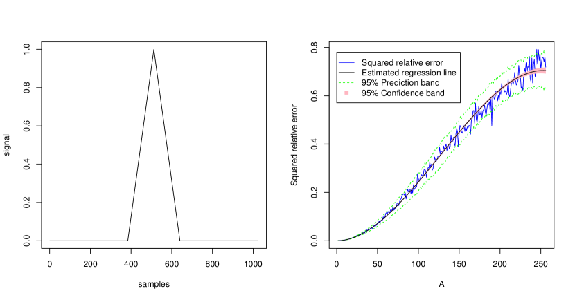
Figure 5. On the left: tent signal $f^{(1)}$ with $N=1024$ samples and support length 256. On the right: squared relative error of the scattering network output for a single realization (blue), third degree polynomial regression curve $\widetilde{f^{(1)}}$ (black) with 95% prediction band (green) and 95% confidence band (pink).

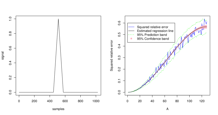
Figure 6. On the left: tent signal $f^{(2)}$ with $N=1024$ samples and support length 128. On the right: squared relative error of the scattering network output for a single realization (blue), third degree polynomial regression curve $\widetilde{f^{(2)}}$ (black) with 95% prediction band (green) and 95% confidence band (pink).

An aspect that glaringly stands out from the figures is the predicted change - in fact a smooth transition - from the quadratic regime to a sublinear one. Moreover, the latter bound justifies in a natural way the detection of the inflection point of the regression line as an empirical measure of the scale $s$ associated with the corresponding subspace $U_{s}=V_{j}$ ($s=2^{j}$) - more precisely, we expect the inflection point to be of the same order of magnitude in base $2$ as $s$.

There are several ways to test this hypothesis. We decided to use a quite simple approach, relying on a polynomial regression model for the squared relative error. From (10.1) we expect the fitting curve to have at most quadratic growth followed by at most linear growth, and the simplest non-trivial model providing for an inflection point is a third degree polynomial $\tilde{f}(x)=a_{0}+a_{1}x+a_{2}x^{2}+a_{3}x^{3}$. In particular, we introduce the estimator $\hat{s}\coloneqq-\widehat{a_{2}}/3\widehat{a_{3}}$ for the inflection point, where $\widehat{a_{2}}$ and $\widehat{a_{3}}$ are the statistics emerging as estimates of the coefficients of $\tilde{f}$. We performed a weighted least squared fit, because of the evident heteroskedasticity of the data - precisely, for each value of $A$, we computed the sample variance over $n=50$ realizations of the network (for each signal) and accordingly weighted the regression model.

As an illustration, we report in Table 1 below the estimated coefficients (with 95% confidence interval) for the polynomial regression and both signals for a single realization. We also provide the adjusted $R^{2}$ statistic and the value of $\hat{s}$ in terms of the fit parameters.

	$\widetilde{f^{(1)}}$		$\widetilde{f^{(2)}}$
	Estimate	$p$ value	Estimate	$p$ value
$a_{0}$	$\displaystyle(-6.999\pm 5.107)\times 10^{-6}$	$0.172$	$(1.097\pm 2.059)\times 10^{-5}$	$0.595$
$a_{1}$	$(-3.239\pm 4.874)\times 10^{-6}$	$0.507$	$(-6.241\pm 2.091)\times 10^{-5}$	$0.003$
$a_{2}$	$(3.303\pm 0.028)\times 10^{-5}$	$<2\times 10^{-16}$	$(1.065\pm 0.002)\times 10^{-4}$	$<2\times 10^{-16}$
$a_{3}$	$(-8.700\pm 0.130)\times 10^{-8}$	$<2\times 10^{-16}$	$(-5.580\pm 0.015)\times 10^{-7}$	$<2\times 10^{-16}$
$R^{2}$	$0.997$		$0.995$
$\hat{s}$	$126.556$		$63.641$

Table 1. Estimated coefficients (with standard deviation and $p$ value) for the third degree polynomial regression model $\widetilde{f}$ for the squared relative error of the scattering network output for a single realization. Adjusted $R^{2}$ statistic is also reported. The value of $\hat{s}=\widehat{a_{2}}/3\widehat{a_{3}}$ can be found in the last line.

The plot of the polynomial regression curve for a single sample realization can be found in Figures 5 and 6 (black). We remark that our model does not achieve a precise fit for large values of $A$; in fact, a fifth degree polynomial regression results in a slightly better fit (also confirmed by ANOVA), while higher order models or even nonlinear ones inspired by (10.1) do not associate with relevant improvement. We prefer to consider here a simpler cubic model in view of the more readily understandable relationship between parameters and inflection point, the estimate of which is our ultimate goal. Let us also emphasize that the estimated coefficients $a_{0}$ and $a_{1}$ are not always statistically significant, as shown in Table 1.

In order to estimate the expectation $\mathbb{E}[\hat{s}]$, polynomial regression is repeated for each sample realization, eventually leading to a collection $\{s_{i}\}_{i=1,\ldots,n}$ of $n=50$ realizations of $\hat{s}$. We report in Table 2 the sample mean $\bar{s}$ of this collection, along with the corresponding sample standard error

$$\sigma=\sqrt{\frac{1}{n(n-1)}\sum_{i=1}^{n}(s_{i}-\bar{s})^{2}}$$

and the 95% confidence interval $(\bar{s}-c\sigma,\bar{s}+c\sigma)$, where $c=2.010$ is the 97.5th percentile of Student’s $t$ distribution with $n-1$ degrees of freedom.

	${f^{(1)}}$	${f^{(2)}}$
$\bar{s}$	$127.144$	$64.019$
$\sigma$	$0.101$	$0.077$
$\mathbb{E}[\hat{s}]$ 95% CI	$(126.942,127.347)$	$(63.864,64.174)$

Table 2. Sample mean $\bar{s}$ over $n=50$ realizations, with sample standard error $\sigma$ and 95% confidence interval $(\bar{s}-c\sigma,\bar{s}+c\sigma)$ with $c=2.010$ (97.5th percentile of Student’s $t$ distribution with $n-1$ degrees of freedom).

Observe that for both signals the estimates come with a relative error (with respect to $s=128$ and $s=64$ respectively) of less than 1%. It is our opinion that this is still a considerable result, in view of the quite unsophisticated design of the experiment. We expect a more careful point of change detection analysis to achieve better results. Also, the same issue seems worth investigating for other multiresolution approximations and for different DCNNs, even in higher dimensions, but this matter is beyond the illustrative purpose of this section and will thus be object of independent consideration in future work.

References

• [1] Rima Alaifari, Giovanni S. Alberti and Tandri Gauksson. ADef: an iterative algorithm to construct adversarial deformations. In: 7th International Conference on Learning Representations, ICLR 2019. Open access: arXiv:1804.07729.
• [2] Charalambos D. Aliprantis, and Kim Border. Infinite dimensional analysis. A hitchhiker’s guide. Springer, 2006.
• [3] Naveed Akhtar and Mian Ajmal. Threat of adversarial attacks on deep learning in computer vision: a survey. IEEE Access 6 (2018): 14410–14430.
• [4] Anish Athalye, Nicholas Carlini and David Wagner. Obfuscated gradients give a false sense of security: circumventing defenses to adversarial examples. In: Proceedings of the 35th International Conference on Machine Learning, PMLR 80:274–283, 2018.
• [5] Radu Balan, Maneesh Singh and Dongmian Zou. Lipschitz properties for deep convolutional networks. Contemporary Mathematics 706 (2018), 129–151.
• [6] Alberto Bietti and Julien Mairal. Invariance and stability of deep convolutional representations. In: Advances in Neural Information Processing Systems (NIPS), 2017.
• [7] Alberto Bietti and Julien Mairal. Group invariance, stability to deformations, and complexity of deep convolutional representations. Journal of Machine Learning Research (JMLR) 20(25) (2019):1–49.
• [8] Joan Bruna and Stéphane Mallat. Invariant scattering convolution networks. IEEE Transactions on pattern analysis and machine intelligence (PAMI), 35(8) (2013), 1872-–1886.
• [9] Nicholas Carlini and David Wagner. Towards evaluating the robustness of neural networks. In: 2017 IEEE Symposium on Security and Privacy (SP), San Jose, CA, USA, 2017, 39–57.
• [10] Elena Cordero and Fabio Nicola. Sharpness of some properties of Wiener amalgam and modulation spaces. Bull. Aust. Math. Soc. 80 (2009), no. 1, 105–116.
• [11] Piero D’Ancona and Fabio Nicola. Sharp $L^{p}$ estimates for Schrödinger groups. Rev. Mat. Iberoam. 32 (2016), no. 3, 1019–1038.
• [12] Lawrence C. Evans. Partial differential equations. Second edition. Graduate Studies in Mathematics, 19. American Mathematical Society, Providence, RI, 2010.
• [13] Hans G. Feichtinger. Banach convolution algebras of Wiener type. In: Functions, series, operators, Vol. I, II (Budapest, 1980), Colloq. Math. Soc. János Bolyai, 35, North-Holland, Amsterdam, 1983, 509–524.
• [14] Hans G. Feichtinger. Banach spaces of distributions of Wiener’s type and interpolation. In: Functional analysis and approximation (Oberwolfach, 1980), Internat. Ser. Numer. Math., 60, Birkhäuser, Basel-Boston, Mass., 1981, 153–165.
• [15] Gerald B. Folland. Real analysis. Modern techniques and their applications. Second edition. Pure and Applied Mathematics (New York). A Wiley-Interscience Publication. John Wiley & Sons, Inc., New York, 1999.
• [16] Ian Goodfellow, Jonathon Shlens and Christian Szegedy. Explaining and harnessing adversarial examples. In: 3rd International Conference on Learning Representations, ICLR 2015. Open access: arXiv:1412.6572.
• [17] Loukas Grafakos. Modern Fourier analysis. Third edition. Graduate Texts in Mathematics. Springer, New York, 2014.
• [18] Karlheinz Gröchenig. Foundations of time-frequency analysis. Applied and Numerical Harmonic Analysis. Birkhäuser Boston, Inc., Boston, MA, 2001.
• [19] Iosif I. Gihman and Anatolij V. Skorohod. The theory of stochastic processes I . Translated from the Russian by Samuel Kotz. Corrected reprint of the first English edition. Grundlehren der Mathematischen Wissenschaften [Fundamental Principles of Mathematical Sciences], 210. Springer-Verlag, Berlin-New York, 1980.
• [20] Philipp Grohs, Thomas Wiatowski and Helmut Bölcskei. Deep convolutional neural networks on cartoon functions. In: 2016 IEEE International Symposium on Information Theory (ISIT), 2016, 1163–1167.
• [21] Douglas Heaven. Why deep-learning AIs are so easy to fool. Nature 574 (2019), 163–166.
• [22] Christopher Heil. An introduction to weighted Wiener amalgams. In: Wavelets and their applications. Ed. by S. Thangavelu, M. Krishna, R. Radha. Allied Publishers, New Dehli, 2003, 183–216.
• [23] Michael Koller, Johannes Großmann, Ullrich Monich and Holger Boche. Deformation stability of deep convolutional neural networks on Sobolev spaces. In: 2018 IEEE International Conference on Acoustics, Speech and Signal Processing (ICASSP), Calgary, AB, 2018, 6872–6876.
• [24] Alexey Kurakin, Ian Goodfellow and Samy Bengio. Adversarial examples in the physical world. In: Artificial Intelligence - Safety and Security, Ed. by R. V. Yampolskiy, Chapman and Hall/CRC, 2018.
• [25] Yann LeCun, Yoshua Bengio and Geoffrey Hinton. Deep learning. Nature 521, (2015), 436–444.
• [26] Heidi Ledford. Millions of black people affected by racial bias in health-care algorithms. Nature 574 (2019), 608–609.
• [27] Aleksander Madry, Aleksandar Makelov, Ludwig Schmidt, Dimitris Tsipras and Adrian Vladu. Towards deep learning models resistant to adversarial attacks. In: 6th International Conference on Learning Representations, ICLR 2018. Open access: arXiv:1706.06083.
• [28] Stéphane Mallat. Group invariant scattering. Comm. Pure Appl. Math. 65 (2012), no. 10, 1331–1398.
• [29] Stéphane Mallat. A wavelet tour of signal processing. The sparse way. Third edition. With contributions from Gabriel Peyré. Elsevier/Academic Press, Amsterdam, 2009.
• [30] David J. Miller, Zhen Xiang and George Kesidis. Adversarial learning targeting deep neural network classification: a comprehensive review of defenses against attacks. Proceedings of the IEEE 108(3) (2020), 402–433.
• [31] Christian Szegedy, Wojciech Zaremba, Ilya Sutskever, Joan Bruna, Dumitru Erhan, Ian Goodfellow and Rob Fergus. Intriguing properties of neural networks. In: 2nd International Conference on Learning Representations, ICLR 2014. Open access: arXiv:1312.6199.
• [32] Terence Tao. Low regularity semi-linear wave equations. Comm. Partial Differential Equations 24 (1999), no. 3-4, 599–629.
• [33] Thomas Wiatowski and Helmut Bölcskei. A mathematical theory of deep convolutional neural networks for feature extraction. IEEE Trans. Inform. Theory 64 (2018), no. 3, 1845–1866.
• [34] Thomas Wiatowski and Helmut Bölcskei. Deep convolutional neural networks based on semi-discrete frames. In: 2015 IEEE International Symposium on Information Theory (ISIT), Hong Kong, China, 2015, 1212–1216.
• [35] Han Xu, Yao Ma, Hao-Chen Liu, Debayan Deb, Hui Liu, Ji-Liang Tang and Anil K. Jain. Adversarial attacks and defenses in images, graphs and text: a review. Int. J. Autom. Comput. 17(2020: 151-–178 .
• [36] Dongmian Zou, Radu Balan and Maneesh Singh. On Lipschitz bounds of general convolutional neural networks. IEEE Trans. on Info. Theory 66(3) (2020), 1738–1759.