Constraining the cosmological parameters using gravitational wave observations of massive black hole binaries and statistical redshift information

Abstract

Space-borne gravitational wave detectors like TianQin are expected to detect gravitational wave signals emitted by the mergers of massive black hole binaries. Luminosity distance information can be obtained from gravitational wave observations, and one can perform cosmological inference if redshift information can also be extracted, which would be straightforward if an electromagnetic counterpart exists. In this paper, we concentrate on the conservative scenario where the electromagnetic counterparts are not available, and comprehensively study if cosmological parameters can be inferred through a statistical approach, utilizing the non-uniform distribution of galaxies as well as the black hole mass-host galaxy bulge luminosity relationship. By adopting different massive black hole binary merger models, and assuming different detector configurations, we conclude that the statistical inference of cosmological parameters is indeed possible. TianQin is expected to constrain the Hubble constant to a relative error of about 4%-7%, depending on the underlying model. The multidetector network of TianQin and LISA can significantly improve the precision of cosmological parameters. In the most favorable model, it is possible to achieve a level of 1.7% with a network of TianQin and LISA. We find that without electromagnetic counterparts, constraints on all other parameters need a larger number of events or more precise sky localization of gravitational wave sources, which can be achieved by the multidetector network or under a favorable model for massive black hole mergers. However, in the optimistic case, where electromagnetic counterparts are available, one can obtain useful constraints on all cosmological parameters in the Lambda cold dark matter cosmology, regardless of the population model. Moreover, we can also constrain the equation of state of the dark energy without the electromagnetic counterparts, and it is even possible to study the evolution of equation of state of the dark energy when the electromagnetic counterparts are observed.

I Introduction

The first direct gravitational wave (GW) detections by Advanced LIGO and Advanced Virgo 2016PhRvL.116f1102A ; 2016PhRvL.116x1103A ; 2017PhRvL.118v1101A ; 2017ApJ…851L..35A ; 2017PhRvL.119n1101A ; 2017PhRvL.119p1101A ; GWTC-1:2018 ; LIGOScientific:2020ibl have opened an era of GW astronomy and the detected GW events have provided powerful tests for astrophysics and fundamental physics LIGOScientific:2018jsj ; 2016ApJ…818L..22A ; 2016PhRvL.116v1101A . The first direct GW detection from a binary neutron star (BNS) merger, GW1708172017PhRvL.119p1101A and its electromagnetic (EM) counterpart identification 2017ApJ…848L..13A ; 2017ApJ…848L..12A provided a “cosmic distance ladder”-free determination of the Hubble constant $H_{0}$ 2017Natur.551…85A ; Hotokezaka:2018dfi . Aside from the GW signals with EM counterpart, GW signals without EM counterpart have also provided effective measurements of $H_{0}$ Fishbach:2018gjp ; 2019ApJ…876L…7S ; Abbott:2019yzh ; Palmese:2020aof , and GWs have become standard sirens for cosmological investigations, as first proposed over thirty years ago 1986Natur.323..310S . There is an especially noticeable tension between local (or so-called late Universe) measurements of the Hubble constant and cosmological (or so-called early Universe) measurements of $H_{0}$ 2016ApJ…826…56R ; Riess:2019cxk ; Freedman:2019jwv ; Aghanim:2018eyx ; Freedman:2017yms ; Verde:2019ivm ; Riess:2020sih ; Riess:2020fzl . The independent determinations of $H_{0}$ from GW detections offer an effective way to clarify this “Hubble tension” Feeney:2018mkj .

The key to the success of the standard siren method involves obtaining redshift information for GW sources. One needs to either (1) identify the EM counterpart and the host galaxy of GW sources, or (2) obtain the statistical redshift distribution of candidate host galaxies, based on our knowledge of galaxy clustering 1986Natur.323..310S . Novel methods have also been developed to obtain the redshift information of GW sources, using such effects/information as 2018SSPMA..48g9805Z : (3) the strong gravitational lensing of GWs Sereno:2010dr ; Sereno:2011ty ; Liao:2017ioi ; (4) the mass distribution function of compact binary GW sources, such as Taylor:2011fs ; Taylor:2012db for BNS and Farr:2019twy ; You:2020wju for stellar-mass binary black hole (StBBH), dependent on our understanding of the history of binary mergers; (5) the redshift probability distribution of compact binary mergers based on their intrinsic merger rates Ding:2018zrk , requiring a large number of GW events and also dependent on our understanding of the history of binary mergers; (6) the phase correction of BNS merger GWs due to tidal effects DelPozzo:2015bna ; Messenger:2011gi ; Messenger:2013fya , requiring detectors with higher sensitivity such as third-generation ground-based GW detectors; (7) the evolution of GW phase with cosmological expansion Seto:2001qf ; Nishizawa:2010xx ; Nishizawa:2011eq , requiring detectors with both higher sensitivity and operating in the decihertz band.

The potential of the second-generation ground-based GW detector network, including Advanced LIGO, Advanced Virgo, KAGRA KAGRA:2018plz and LIGO-India LIGO-India:2013 , to measure $H_{0}$ has been studied in detail, e.g., the measurements of $H_{0}$ from BNS merger GW detections Fishbach:2018gjp ; Taylor:2011fs ; Nissanke:2013fka ; Mortlock:2018azx ; Chen:2017rfc , measuring $H_{0}$ with neutron star black hole mergers Vitale:2018wlg and the constraints on $H_{0}$ via StBBH mergers GW detections Chen:2017rfc ; DelPozzo:2012zz ; Nair:2018ign ; Farr:2019twy ; Gray:2019ksv .

Third-generation ground-based GW detectors such as the Einstein Telescope (ET) Punturo:2010zz and Cosmic Explorer (CE) Evans:2016mbw are expected to detect thousands of GW events with a redshift concentration at $z\approx 2$ and a horizon of $z\approx 10$ Sathyaprakash:2009xt ; Taylor:2012db ; deSouza:2019ype ; Ding:2018zrk . The high-redshift GW events detected by ET or CE can provide precise measurements of $H_{0}$ and other cosmological parameters, such as the density of dark matter $\Omega_{M}$, and of dark energy $\Omega_{\Lambda}$ Nair:2018ign ; Taylor:2012db ; Ding:2018zrk ; You:2020wju ; Zhao:2010sz ; DelPozzo:2015bna ; Cai:2016sby ; Zhang:2018byx ; Du:2018tia ; Yu:2020vyy . In addition, a large number of high-redshift GW events would allow us to reconstruct the dark energy equation of state (EoS) and expansion dynamics by nonparametric methods Seikel:2012uu ; Cai:2016sby ; Yang:2019vni .

Space-borne GW detectors like TianQin will open for exploration the millihertz to Hertz band of the GW spectrum. TianQin is a constellation of three satellites orbiting around the Earth, using drag-free control to lower noise and measure GW effects through laser interferometry Luo:2015 ; Mei:2020lrl . TianQin is expected to observe multiple different types of GW source, including StBBH inspiralsLiu:2020eko , extreme mass ratio inspirals Fan:2020zhy , Galactic compact binaries Huang:2020rjf and massive black hole binary (MBHB) mergers Wang:2019 . Such detections are also expected to put stringent constraints on deviations from general relativity or testing specific gravity theories Shi:2019hqa ; Bao:2019kgt . Studies have revealed the availability of stable orbits that fulfils the requirement for GW detections Zhang:2020paq ; Ye:2020tze ; Tan:2020xbm ; Ye:2019txh . Moreover, the technology demonstration satellite, TianQin-1, has met the design requirements Luo:2020bls .

Studies have been performed on the ability of GWs observations to constrain cosmological models with the Laser Interferometer Space Antenna (LISA) Holz:2005df ; Dalal:2006qt ; LISA:2017pwj ; Arun:2008xf ; Babak:2010ej ; 2016JCAP…04..002T ; Caprini:2016qxs ; Cai:2017yww ; Wang:2020dkc . GWs can usefully constrain cosmology even when no EM information is available, according to studies carried out on the measurement of $H_{0}$ with MBHB mergers Petiteau:2011we ; Wang:2020dkc , StBBH inspirals Kyutoku:2016zxn ; DelPozzo:2017kme , and EMRIs macleod2008precision ; Laghi:2021pqk . Next generation missions like the Decihertz Interferometer Gravitational Wave Observatory (DECIGO) Kawamura:2006up and the Big Bang Observer (BBO) Crowder:2005nr can also serve as powerful cosmological probes Nishizawa:2010xx ; Nishizawa:2011eq ; Namikawa:2015prh .

In this paper, we focus on the ability of space-borne GW detectors to constrain the cosmological parameters using MBHB merger GW signals. Some studies have suggested that MBHB mergers may have observable electromagnetic signatures Armitage:2002uu ; Palenzuela:2010nf ; Gold:PRD2014 ; Farris:mnrasl2014 , and some thus assume the availability of an EM counterpart when performing GW cosmology studies Holz:2005df ; Arun:2008xf ; 2016JCAP…04..002T ; Cai:2017yww ; Wang:2019tto ; Wang:2021srv . In order to be conservative, however, we set as our default assumption that no EM counterparts are detectable for our GW sources, so that we rely on the luminosity distance information from the GW detections combined with statistical information about their host galaxy redshifts to constrain the cosmological parameters. Our method can be simply described as follows: GW detection provides a localisation error cone for the three-dimensional (3D) position of the GW source; one can use the redshift distribution of the galaxies within the cone as the proxy for the GW redshift. However, there could be a lot of galaxies within the localisation error volume that will cause contamination and limit the effectiveness of the dark standard siren method. We therefore study how using the relationship between the central massive black holes and their host galaxies Graham:2007uq ; Bentz:2008rt ; Kormendy:2013dxa ; Jiang:2011bt can better pinpoint the host and improve the cosmological estimation. We study this under the assumption that both TianQin Luo:2015 and LISA LISA:2017pwj ; Robson:2019 will be operating in the 2030s, with overlapping operation time and the scope for joint detections.

The remainder of this paper is organized as follows. In Sec. II, we present the appropriate cosmology theory and introduce the astrophysical background needed for our analysis. In Sec. III, we present the simulation method used to generate our observations and describe the characteristics of our simulated data. In Sec. IV, we show the results of our constraints on the cosmological parameters. In Sec. V, we discuss several key issues in our simulations. Finally, in Sec. VI, we summarize our findings.

II Methodology

II.1 The cosmological models

Throughout this paper, we consider a Universe in which the spacetime can be described by the Friedmann-Lemaître-Robertson-Walker metric, and adopt the Lambda cold dark matter ($\Lambda$CDM) model as our fiducial model, with the dark energy EoS being described by a constant $\omega\equiv p_{\Lambda}/\rho_{\Lambda}=-1$. In this model the expansion of the Universe can be characterized by the Hubble parameter $H(z)\equiv\dot{a}/a$, with $a$ being the scale factor, the current value of which is $a_{0}$, and with redshift $z$ defined as $z+1\equiv a_{0}/a$. The Hubble parameter can therefore be expressed as

$$H(z)=H_{0}\sqrt{\Omega_{M}(1+z)^{3}+\Omega_{K}(1+z)^{2}+\Omega_{\Lambda}},$$ (1)

where the Hubble constant $H_{0}\equiv H(z=0)$ describes the current expansion rate of the Universe, and $\Omega_{M}$, $\Omega_{K}$ and $\Omega_{\Lambda}$ are respectively the current dimensionless fractional densities for the total matter, curvature and dark energy with respect to the critical density. They satisfy the relationship $\Omega_{M}+\Omega_{K}+\Omega_{\Lambda}\equiv 1$.

We will also consider the possibility that the dark energy component has dynamical properties, by adopting the Chevallier-Polarski-Linder (CPL) parametrization Chevallier:2000qy ; Linder:2002et

$$\omega(z)=w_{0}+w_{a}\frac{z}{1+z}.$$ (2)

This yields the equation

$$H(z)=H_{0}\sqrt{\Omega_{M}(1+z)^{3}+\Omega_{K}(1+z)^{2}+\Omega_{\Lambda}\exp\Big{(}-\frac{3w_{a}z}{1+z}\Big{)}(1+z)^{3(1+w_{0}+w_{a})}}.$$ (3)

Estimates of the cosmological parameters can be inferred by fitting the relationship between observed luminosity distances $D_{L}$ and redshifts $z$. This relationship encodes information about the expansion history of universe, and is given by

$$D_{L}=\frac{c(1+z)}{H_{0}}\left\{\begin{array}[]{ll}\frac{1}{\sqrt{\Omega_{K}}}\sinh[\sqrt{\Omega_{K}}\int_{0}^{z}\frac{H_{0}}{H(z^{\prime})}dz^{\prime}]&\textrm{for $\Omega_{K}>0$}\\ \int_{0}^{z}\frac{H_{0}}{H(z^{\prime})}dz^{\prime}&\textrm{for $\Omega_{K}=0$}\\ \frac{1}{\sqrt{|\Omega_{K}|}}\sin[\sqrt{|\Omega_{K}|}\int_{0}^{z}\frac{H_{0}}{H(z^{\prime})}dz^{\prime}]&\textrm{for $\Omega_{K}<0$}\end{array}\right.$$ (4)

where $c$ is speed of light in vacuum.

We adopt cosmological parameters derived from various recent observations, like Planck Aghanim:2018eyx , $H_{0}=67.8$ km/s/Mpc, $\Omega_{M}=0.307$, $\Omega_{\Lambda}=0.693$ and we adopt $w_{0}=-1$, $w_{a}=0$, respectively, consistent with the observed galaxy distribution Klypin2016 .

II.2 Standard sirens

For the inspiral of a compact binary system with component masses $m_{1}$ and $m_{2}$, the frequency domain GW waveform can be expressed as Sathyaprakash:2009xs

$$\widetilde{h}(f)=\frac{1}{D_{L}}\sqrt{\frac{5}{24}}\frac{(G{\mathcal{M}_{z}})^{5/6}}{\pi^{2/3}c^{3/2}}f^{-7/6}\exp\big{(}-i\Phi(f;\mathcal{M}_{z},\eta)\big{)}$$ (5)

where $G$ is the gravitational constant, $\mathcal{M}=\eta^{3/5}M$ is the chirp mass, $\eta=m_{1}m_{2}/M^{2}$ is the symmetric mass ratio, $M=m_{1}+m_{2}$ is the total mass, and $\Phi(f;\mathcal{M}_{z},\eta)$ is phase of the waveform depending on the parameters $\mathcal{M}$ and $\eta$. The chirp mass $\mathcal{M}$ largely determines the overall evolution of the GW waveform, but the parameter directly measured from the data is actually the redshifted chirp mass $\mathcal{M}_{z}\equiv\mathcal{M}(1+z)$.

One can see from Eq. (5) that the luminosity distance $D_{L}$ of the binary has a direct impact on the measured waveform amplitude. Therefore, GW observations of compact binary coalescences can be used to estimate their corresponding luminosity distance directly. If the redshifts of such mergers can be inferred through other observational or theoretical channels, one can use information from both luminosity distance and redshift to constrain the cosmological parameters 1986Natur.323..310S . Such a one-stop measurement of luminosity distance makes the inspiral signal of compact binary systems desirable objects for cosmological studies, since they are largely immune to systematic errors caused by intermediate calibration stages like those required by type Ia supernovae; consequently, they have been coined as “standard sirens” .

There is a catch, however. Both $D_{L}$ and $z$ are needed in order to use Eq. (4) to infer cosmological parameters. Moreover, as noted above, the redshift $z$ is deeply intertwined with the chirp mass $\mathcal{M}$ and can not be solely determined by GW observations of the inspiral. The measurement of redshift information thus relies on extra information, like the identification of the host galaxy or the direct observation of an EM counterpart.

II.3 Bayesian framework

We adopt a Bayesian framework to infer cosmological parameters through the GW observations of massive black hole binary mergers. Consider a set of data composed of $N$ GW observations, $D\equiv\{D_{1},D_{2},...,D_{i},...,D_{N}\}$, as well as an EM data set $S$ derived from EM observations. Then one can derive the posterior probability distribution of the cosmological parameters $\vec{\Omega}$ as

$$p(\vec{\Omega}|D,S,I)=\frac{p_{0}(\vec{\Omega}|I)p(D,S|\vec{\Omega},I)}{p(D,S|I)}=\frac{p_{0}(\vec{\Omega}|I)\prod_{i}p(D_{i},S|\vec{\Omega},I)}{p(D,S|I)},$$ (6)

where $I$ indicates all relevant background information. Since the normalisation factor, also known as the Bayesian evidence, $p(D,S|I)$, is irrelevant in the calculation, the posterior can be written as

$$p(\vec{\Omega}|D,S,I)\varpropto p_{0}(\vec{\Omega}|I)\prod_{i}p(D_{i},S|\vec{\Omega},I).$$ (7)

We can classify parameters into three categories: the common parameters (which affect both GW waveforms and EM observations); GW-only parameters $\vec{\theta}^{\prime}$, and EM-only parameters $\vec{\phi}^{\prime}$. Throughout this paper, we identify the common parameters as the luminosity distance $D_{L}$, the redshift $z$, the longitude $\alpha$, the latitude $\delta$, the total mass $M$ of the compact binary, and the bulge luminosity $L_{\rm bulge}$ of the host galaxy. We can express the likelihood as

$$p(D_{i},S|\vec{\Omega},I)=\frac{\int p(D_{i},S,D_{L},z,\alpha,\delta,M_{z},L_{\rm bulge},\vec{\theta}^{\prime},\vec{\phi}^{\prime}|\vec{\Omega},I)dD_{L}dzd\alpha d\delta dM_{z}dL_{\rm bulge}d\vec{\theta}^{\prime}d\vec{\phi}^{\prime}}{\beta(\vec{\Omega}|I)},$$ (8)

where $M_{z}=M(1+z)$ is the redshifted total mass of the GW source. Notice that we introduce a correction term $\beta(\vec{\Omega}|I)$ to eliminate the effect of selection biases 2017Natur.551…85A ; Chen:2017rfc ; Mandel:2018mve . The integrand in the numerator of Eq. (8) can be factorized as

$$p(D_{i},S,D_{L},z,\alpha,\delta,M_{z},L_{\rm bulge},\vec{\theta}^{\prime},\vec{\phi}^{\prime}|\vec{\Omega},I)$$

$$=\!~{} p(D_{i}|D_{L},\alpha,\delta,M_{z},\vec{\theta}^{\prime},I)p(S|z,\alpha,\delta,L_{\rm bulge},\vec{\phi}^{\prime},I)p_{0}(D_{L}|z,\vec{\Omega},I)p_{0}(M_{z}|z,L_{\rm bulge},\vec{\Omega},I)$$

$$\!\!\times p_{0}(z,\alpha,\delta,L_{\rm bulge}|\vec{\Omega},I)p_{0}(\vec{\theta}^{\prime}|\vec{\Omega},I)p_{0}(\vec{\phi}^{\prime}|\vec{\Omega},I).$$ (9)

For details on the derivation of Eq. (II.3), please refer to Appendix A. The general mathematical treatment of the likelihood $p(D_{i}|D_{L},\alpha,\delta,M_{z},\vec{\theta}^{\prime},I)$ can be given by Finn:1992

$$p(D_{i}|D_{L},\alpha,\delta,M_{z},\vec{\theta}^{\prime},I)\varpropto\exp\Big{[}-\frac{1}{2}\big{\langle}D_{i}-h(D_{L},\alpha,\delta,M_{z},\vec{\theta}^{\prime})|D_{i}-h(D_{L},\alpha,\delta,M_{z},\vec{\theta}^{\prime})\big{\rangle}\Big{]},$$ (10)

where $\langle\cdot|\cdot\rangle$ is the inner product as defined in Eq. (22). When the host galaxy of the GW signal cannot be uniquely identified, one can set $p(S|z,\alpha,\delta,L_{\rm bulge},\vec{\phi}^{\prime},I)$ as a constant Chen:2017rfc . We assume that $p_{0}(D_{L}|z,\vec{\Omega},I)\equiv\delta\big{(}D_{L}-\hat{D}_{L}(z,\vec{\Omega})\big{)}$ depends on the cosmological model and $p_{0}(M_{z}|z,L_{\rm bulge},\vec{\Omega},I)\equiv\delta\big{(}M_{z}-(1+z)\hat{M}(L_{\rm bulge})\big{)}$ is based on the relation of massive black hole mass with galactic luminosity Bentz:2008rt ; Kormendy:2013dxa , where the total mass $\hat{M}(L_{\rm bulge})$ is a function of the galactic bulge luminosity $L_{\rm bulge}$.

The EM measurements of parameters like position of the galaxies $(\alpha,\delta)$ are much more precise compared with the measurements from GW observations. The prior in Eq. (II.3) can therefore be approximated as Chen:2017rfc ; Petiteau:2011we ; DelPozzo:2012zz

$$p_{0}(z,\alpha,\delta,L_{\rm bulge}|\vec{\Omega},I)=\frac{1}{N_{\rm gal}}\sum_{j=1}^{N_{\rm gal}}\mathcal{N}(z|{\bar{z}^{j}},\sigma_{z}^{j})\delta(\alpha-\alpha^{j})\delta(\delta-\delta^{j})\mathcal{N}(L_{\rm bulge}|\bar{L}_{\rm bulge}^{j},\sigma_{L_{\rm bulge}}^{j}),$$ (11)

where $N_{\rm gal}$ is the number of galaxies in our EM catalog, and $\mathcal{N}(x|\bar{x},\sigma_{x})$ is a Gaussian distribution on $x$, with expectation $\bar{x}$ and standard deviation $\sigma_{x}$, here $x=\{z,L_{\rm bulge}\}$. However, if the luminosity function $\Phi(L)$ is also regarded as redshift-dependent (as in Cohen:2001ag ; Marchesini:2006vg ; Bouwens:2014fua etc.), then Eq. (11) needs to be supplemented, as shown in Eq. (III.4).

Marginalizing over the parameters $D_{L}$, $M_{z}$, $\vec{\theta}^{\prime}$, and $\vec{\phi}^{\prime}$, Eq. (8) becomes

$$p(D_{i},S|\vec{\Omega},I)\varpropto\frac{\int p\big{(}D_{i}|\hat{D}_{L}(z,\vec{\Omega}),\alpha,\delta,(1+z)\hat{M}(L_{\rm bulge}),I\big{)}p_{0}(z,\alpha,\delta,L_{\rm bulge}|\vec{\Omega},I)dzd\alpha d\delta dL_{\rm bulge}}{\beta(\vec{\Omega}|I)}.$$ (12)

We next examine the correction term $\beta(\vec{\Omega}|I)$. Bias of the inferred cosmological parameters might arise from two sources: the GW data and the EM information. The EM information contains the following bias: (1) the 3D error volume is cone like, so this will in general lead to a bias towards higher redshift due to the larger associated volume; and (2) the incompleteness of the catalog will introduce a Malmquist bias, where brighter galaxies are disproportionately recorded and weighted 1922MeLuF.100….1M . To obtain cosmological constraints from “dark” standard sirens depends on the non-uniform distribution of galaxies, due to large scale structures (LSS) or smaller-scale clustering of galaxies, so the correction term should exclude the influence of LSS and galaxy clustering information as far as possible. We account for the aforementioned two biases by counting the detectable galaxies over the whole sky, and considering the redshift evolution of this galaxy count. We assume that the EM observations are isotropic within the survey region, and define the prior for the redshift distribution of galaxy catalog as

$$p_{\textrm{c}}(z|\vec{\Omega},I)\varpropto\frac{1}{2\Delta z}\int_{(z-\Delta z)}^{(z+\Delta z)}\int\!\!\!\!\int_{4\pi}\int p_{0}(z^{\prime},\alpha,\delta,L_{\rm bulge}|\vec{\Omega},I)dL_{\rm bulge}d\alpha d\delta dz^{\prime},$$ (13)

where $\Delta z$ is chosen to be much larger than the typical redshift scale of the LSS. The correction term after marginalization is then

$$\beta(\vec{\Omega}|I)\approx\int p(D_{i}|\hat{D}_{L}(z,\vec{\Omega}),I)p_{\textrm{c}}(z|\vec{\Omega},I)dz.$$ (14)

Notice that the GW selection effect is accounted for by integrating over only events detectable by GW detectors. In addition, if the catalog of survey galaxies contains two or more sky areas with different observation depths, then $p_{\textrm{c}}(z|\vec{\Omega},I)$ and $\beta(\vec{\Omega}|I)$ terms need to be calculated separately for each sky area.

For our analysis, the incompleteness of a galaxy catalog can introduce two effects. First, it could bring Malmquist bias so that more distant galaxies are disproportionately weighted. Such a systematic bias is caused by the selection effect that a catalog tends to be more complete for brighter galaxies. The correction term $\beta(\vec{\Omega}|I)$ accounts for this bias. On the other hand, a less complete catalog means there is a higher chance for the host galaxy cluster to be missed. In this case, an additional bias could be introduced to the analysis. In Sec. V.5 we demonstrate that such a large deviation can be identified through application of a consistency check. Meanwhile, in Gray:2019ksv the authors take a step further than Eq. (14), so that more distant events are down-weighted and a consistency check is considered unnecessary.

II.4 Parameter estimation of the GW sources

We define the sensitivity curve $S_{n}(f)$ in terms the expected power spectral density $S_{N}(f)$ according to the relation,

$$S_{n}(f)=\frac{S_{N}(f)}{\bar{\mathcal{T}}(f)},$$ (15)

where $\bar{\mathcal{T}}(f)$ is the sky and polarization averaged response function of the detector,

$$\bar{\mathcal{T}}(f)\approx\frac{1}{1+0.6{(2\pi fL/c)}^{2}},$$ (16)

and

$$S_{N}(f) =\frac{1}{L^{2}}\bigg{[}\frac{4S_{a}}{(2\pi f)^{4}}\left(1+\frac{10^{-4}\textrm{Hz}}{f}\right)+S_{x}\bigg{]}+S_{c}(f), \rm{for\ TianQin},$$ (17)

$$S_{N}(f) =\frac{1}{L^{2}}\bigg{[}\frac{4S_{a}}{(2\pi f)^{4}}\bigg{(}1+\Big{(}\frac{4\times 10^{-4}\textrm{Hz}}{f}\Big{)}^{2}\bigg{)}+S_{x}\bigg{]}+S_{c}(f), \rm{for\ LISA}.$$ (18)

Here $L$ is the arm length, $S_{a}$ is the acceleration noise, $S_{x}$ is the positional noise, and $S_{c}(f)$ is the Galactic foreground noise. For TianQin, $S_{a}^{1/2}=1\times 10^{-15}~{}\textrm{m}\ \textrm{s}^{-2}\textrm{Hz}^{-1/2}$, $S_{x}^{1/2}=1\times 10^{-12}~{}\textrm{m}\ \textrm{Hz}^{-1/2}$, and the arm-length $L=\sqrt{3}\times 10^{8}~{}\textrm{m}$ Luo:2015 ; Wang:2019 ; for LISA, we adopt $S_{a}^{1/2}=3\times 10^{-15}~{}\textrm{m}\ \textrm{s}^{-2}\textrm{Hz}^{-1/2}$, $S_{x}^{1/2}=1.5\times 10^{-11}~{}\textrm{m}\ \textrm{Hz}^{-1/2}$, and arm length $L=2.5\times 10^{9}~{}\textrm{m}$ Robson:2019 . In addition, we added the Galactic foreground on top of the sensitivity curve assuming an observation time of 4 years according to Robson:2019 . On the other hand, no foreground is added for TianQin and it has been suggested that the anticipated foreground will be below TianQin’s sensitivity Huang:2020rjf ; Liang:2021bde . The sky- and polarization-averaged sensitivity curves of TianQin and LISA are shown in Fig. 1.

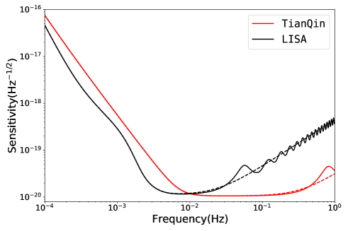
Figure 1: Anticipated averaged sensitivity curves of TianQin (red line) and LISA (black line). Base on Eqs. (17) and (18).

A simultaneous observation from multiple detectors can improve the sky localisation of the GW source. Specifically, the long baseline between different GW detectors makes it possible to use the time delay information to perform sky localisation 2017PhRvL.119n1101A ; 2017PhRvL.119p1101A ; GWTC-1:2018 ; 2017Natur.551…85A ; Wang:2020dkc ; Ruan:2020smc .

Suppose that the $k$th detector record the GW strain $h^{k}(t)$, the strain takes the form

$$h^{k}(t)=\frac{1+\cos^{2}\iota}{2}A(t)\cos\!\big{[}\Phi(t)+\Phi_{D}^{k}(t)+\Phi_{P}^{k}(t)\big{]}F_{+}^{k}(t)+\cos\iota~{}A(t)\sin\!\big{[}\Phi(t)+\Phi_{D}^{k}(t)+\Phi_{P}^{k}(t)\big{]}F_{\times}^{k}(t)$$ (19)

where $\iota$ is the source inclination angle, $A(t)$ and $\Phi(t)$ are the amplitude and phase of the GW respectively, $F_{+,\times}^{k}(t)$ are the response functions of the $k$th detector, $\Phi_{D}^{k}(t)$ is the Doppler frequency modulation due to the Doppler effect of the solar orbital revolution of the detector, and $\Phi_{P}^{k}(t)$ is the phase modulation. The expressions for the phase modulation and the response function are closely related to the orbit of the detectors. We follow Wang:2019 ; Hu:2018 for TianQin, and Cutler:1998 ; 2003PhRvD..67b2001C for LISA, adopting the low-frequency limit.

For a circularised binary black hole merger event, the GW signal can be generally described by a set of parameters including the binary component masses $m_{1}$ and $m_{2}$ (which can be reexpressed as chirp mass $\mathcal{M}$ and symmetric mass ratio $\eta$), the luminosity distance $D_{L}$, the longitude $\alpha$ and latitude $\delta$ of the source sky position, the coalescence phase $\phi_{c}$, the coalescence time $t_{c}$, and the direction of the orbital angular momentum of the GW source $(\alpha_{L},\delta_{L})$ (which can be reexpressed as an inclination angle $\iota$ and polarization angle $\psi$). More parameters would be needed if the spins of the black holes are included.

Let us consider a detector network including $N$ independent detectors, for which the frequency domain GW signal $\widetilde{\bm{h}}(f)$ can be written as

$$\widetilde{\bm{h}}(f)=\Big{[}\widetilde{h}^{1}(f),\widetilde{h}^{2}(f),\cdots,\widetilde{h}^{k}(f),\cdots,\widetilde{h}^{N}(f)\Big{]}^{\rm T}$$ (20)

where $\widetilde{h}^{k}(f)$ denotes the Fourier transform of $h^{k}(t)$. The signal-to-noise ratio (SNR) $\rho$ of a GW signal $\widetilde{\bm{h}}(f)$ can be defined as Finn:1992 ; Cutler:1994

$$\rho=\langle\widetilde{\bm{h}}(f)|\widetilde{\bm{h}}(f)\rangle^{1/2},$$ (21)

where the inner product symbol $\langle\cdot|\cdot\rangle$ is defined as

$$\langle\widetilde{\bm{h}}(f)|\widetilde{\bm{h}}(f)\rangle=\sum_{k}\langle\widetilde{h}^{k}(f)|\widetilde{h}^{k}(f)\rangle\equiv\sum_{k}4\mathfrak{Re}\int_{0}^{\infty}\frac{\widetilde{h}^{k*}(f)\widetilde{h}^{k}(f)}{S_{n}^{k}(f)}df,$$ (22)

where $*$ represents complex conjugate, $\mathfrak{Re}$ denotes the real component, and $S_{n}^{k}(f)$ are the sensitivity curve functions of the $k$th detector respectively when the response functions $F_{+,\times}(t)$ adopt the low-frequency approximation Wang:2019 ; Robson:2019 .

For a GW signal from a binary characterised by physical parameters $\bm{\theta}=(\mathcal{M},\eta,D_{L},\alpha,\delta,\cos\iota,\psi,\phi_{c},t_{c})$, the inverse of the corresponding Fisher information matrix (FIM) sets the Cramér-Rao lower bound for the covariance matrix Vallisneri_2008 . The FIM can be written as

$$\Gamma_{mn}\equiv\bigg{\langle}\frac{\partial\widetilde{\bm{h}}(f)}{\partial\theta_{m}}\bigg{|}\frac{\partial\widetilde{\bm{h}}(f)}{\partial\theta_{n}}\bigg{\rangle},$$ (23)

where $\theta_{m}$ indicates the $m$th parameter. With $\Sigma=\Gamma^{-1}$, we take the estimation uncertainty on parameter $\theta_{m}$ as $\Delta\theta_{m}=\sqrt{\Sigma_{mm}}$, with the sky localization error $\Delta\Omega$ given by the combination $\Delta\Omega=2\pi|\sin\delta|\sqrt{\Sigma_{\alpha\alpha}\Sigma_{\delta\delta}-\Sigma_{\alpha\delta}^{2}}$.

If the GW signals are gravitationally lensed, or the peculiar velocity of its host galaxy is not properly accounted for, the inferred luminosity distance would be in error. Therefore, in addition to the measurement error from GW observation, weak lensing and peculiar velocity can both contribute to the intrinsic uncertainty of the estimated $D_{L}$. We denote $\sigma_{D_{L}}^{\textrm{GW}}$ as the uncertainty arising from the GW observation, and $\sigma_{D_{L}}^{\textrm{tot}}$ as the overall uncertainty including all sources of error. We adopt a fitting formula from Hirata:2010ba (also see Cusin:2020ezb ) to estimate the weak lensing error $\sigma_{D_{L}}^{\textrm{lens}}$, given by

$$\sigma_{D_{L}}^{\textrm{lens}}(z)=\frac{1}{2}D_{L}(z)\sigma_{\ln D_{L}^{2}}=\frac{1}{2}D_{L}(z)\times C_{l}\bigg{[}\frac{1-(1+z)^{-\beta_{l}}}{\beta_{l}}\bigg{]}^{\alpha_{l}},$$ (24)

where $C_{l}=0.066$, $\beta_{l}=0.25$ and $\alpha_{l}=1.8$. For the error, $\sigma_{D_{L}}^{\rm pv}$, due to peculiar velocity we adopt the fitting formula from Kocsis:2005vv ; Gordon:2007zw ,

$$\sigma_{D_{L}}^{\rm pv}(z)=D_{L}(z)\times\bigg{[}1+\frac{c(1+z)^{2}}{H(z)D_{L}(z)}\bigg{]}\frac{\sqrt{\langle v^{2}\rangle}}{c},$$ (25)

with $\sqrt{\langle v^{2}\rangle}=500\ \textrm{km}/\textrm{s}$ as the root mean square peculiar velocity of the host galaxy with respect to the Hubble flow He:2019dhl . We then define the total uncertainty

$$\sigma_{D_{L}}^{\textrm{tot}}=\sqrt{(\sigma_{D_{L}}^{\textrm{GW}})^{2}+(\sigma_{D_{L}}^{\textrm{lens}})^{2}+(\sigma_{D_{L}}^{\rm pv})^{2}},$$ (26)

Throughout this paper, we use $\sigma_{D_{L}}^{\textrm{tot}}$ for our likelihood calculation. However, we remark that the above is a conservative estimate of the total uncertainty, since “delensing” methods like the use of weak lensing maps Shapiro:2010MNRAS , observations of the foreground galaxies Jonsson:2006vc or deep shear surveys Hilbert:2010am could in principle be used to alleviate $\sigma_{D_{L}}^{\textrm{lens}}$, while peculiar velocity maps could also be used to reduce $\sigma_{D_{L}}^{\rm pv}$ 2017Natur.551…85A ; Howlett:2019mdh . We do not apply such corrections in this paper; hence we can expect better results for GW cosmological inference from realistic future detections.

III Simulations

For the purpose of our paper, we require a catalog of massive black hole mergers that mimic our understanding of the real Universe. In this section, we describe the simulation of these catalogs, and how we use the 3D localisation information derived from a GW detection, as well as the empirical $M_{\rm MBH}-L_{\rm bulge}$ relation, to allocate probabilities to candidate host galaxies.

III.1 Massive black hole binary mergers and galaxy catalog

Following previous studies, e.g., Klein:2016 ; Wang:2019 , we adopt the massive black hole binary merger populations from 2012MNRAS.423.2533B . Both the “light-seed” scenario and the “heavy-seed” scenario are considered for the seeding models of massive black holes. In the light-seed scenario, seed black holes are assumed to be the remnants of first generation (or population III) stars and the mass of the seed black hole is around 100 $M_{\odot}$ Madau:2001sc ; Volonteri:2002vz . This model is later referred to as popIII. In the heavy-seed scenario, the MBH seeds are assumed to be born from the direct collapse of protogalactic disks that may be driven by bar instabilities Klein:2016 , with a mass of $\sim 10^{5}~{}M_{\odot}$. The critical Toomre parameter $Q$ that determines when the protogalactic disks become unstable is set to 3 Volonteri:2007ax . Two models are derived from this scenario, with Q3d considering the time lag between the merger of MBHs and merger of galaxies, and Q3nod, which does not consider such a time lag. In both scenarios, the seed BHs grow via accretion and mergers, eventually becoming the massive black holes, while the evolution of MBHs are deeply coupled to the evolution of their host galaxies Ferrarese:2000se .

In addition to the simulated catalog of GW mergers, we also require a simulated galaxy catalog, so that we can associate each MBHB merger with a certain host galaxy and use multimessenger information to infer cosmological parameters. TianQin has the ability of observing very distant mergers, but no existing galaxy survey project can extend to these distances so we choose to adopt the MultiDark Planck (MDPL) cosmological simulation Klypin2016 from the Theoretical Astrophysical Observatory (TAO) TAO-web for this purpose. The MDPL simulated a catalog of galaxies based on an $N$-body simulation which tracks the evolution of dark matter halos assuming a Planck cosmology Ade:2015xua , with $3840^{3}$ particles and a box side length to $h^{-1}$ Gpc (where $h\equiv\frac{H_{0}}{100\ \textrm{km/s/Mpc}}$), and the simulation is performed from $z=100$ to $z=0$. Additional information such as galaxy evolution was obtained from the semi-analytic galaxy evolution model Croton:2016etl , and the luminosity distribution from Conroy et al. Conroy:2009gw .

III.2 GW event catalog

We first simulated MBHB mergers according to the three models (popIII, Q3d, and Q3nod), where only events with network SNR $\rho>8$ are later used. Notice that although TianQin has the ability to observe very distant events, it is anticipated that complete galaxy catalogs would be extremely hard to obtain for galaxies beyond redshift $z=3$, therefore we apply a redshift cut beyond this point. The remaining parameters are then generated from simple distributions: all angle parameters are chosen uniformly in solid angle, $\alpha\in\textrm{U}[0,2\pi]$, $\cos\delta\in\textrm{U}[-1,1]$, $\alpha_{L}\in\textrm{U}[0,2\pi]$, and $\cos\delta_{L}\in\textrm{U}[-1,1]$, and we choose the merger time $t_{c}\in\textrm{U}[0,5]$ years, merger phase $\phi_{c}\in\textrm{U}[0,2\pi]$ and the spin $\chi_{1,2}\in\textrm{U}[-1,1]$. Based on these parameters, we generate the GW waveform from the IMRPhenomPv2 model Hannam:2014 .

Throughout this analysis, we consider multiple configurations for the space-borne GW detectors as described below:

• (i) TianQin: the default case where three satellites form a constellation and operate in a “3 month on + 3 month off” mode, with a mission life time of 5 years Luo:2015 ;

• (ii) TianQin I+II: a twin constellation of satellites are used that have perpendicular orbital planes to avoid the 3-month gaps in data Wang:2019 ; Liu:2020eko ;

• (iii) LISA: we consider the mission as described in LISA:2017pwj ; Robson:2019 , with a nominal mission life time of 4 years;

• (iv) TianQin+LISA: TianQin and LISA observing together, with 4 years of overlap in operation time;

• (v) TianQin I+II+LISA: similar to above but with the TianQin I+II configuration considered.

Previous work indicates that both TianQin Wang:2019 and LISA Klein:2016 have good detection capabilities for MBHB mergers. In Table I we list the anticipated total detection rates for mergers at redshift $z<3$ under different detector configurations. It is worth noting that the actual merger rate of MBHB is likely to increase by about twice as much as the three population models predict Klein:2016 , and our actual detection rate would therefore also likely increase by about twice as much.

Table I: Expected total detection rate of GW events with $z<3$ and SNR $\rho>8$, detected over the entire observation time based on the MBHB population models for five different detector configurations: TianQin, TianQin I+II, LISA, TianQin+LISA, and TianQin I+II+LISA.

	popIII		Q3d		Q3nod
Detectors configuration	Detection rate	Detection percentage	Detection rate	Detection percentage	Detection rate	Detection percentage
TianQin	7.7	33.0%	4.1	32.6%	25.5	26.8%
TianQin I+II	12.0	51.4%	7.2	56.6%	41.8	44.0%
LISA	11.1	61.0%	6.5	64.2%	37.8	50.8%
TianQin+LISA	14.0	68.1%	8.0	71.0%	46.9	56.4%
TianQin I+II+LISA	15.6	72.3%	9.1	75.9%	53.0	60.2%

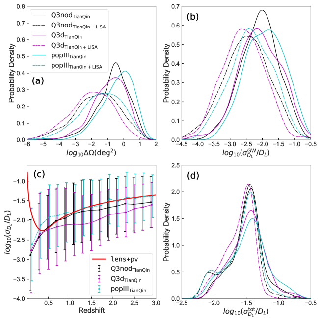
Figure 2: Spatial localisation error distribution for TianQin (solid line) and the LISA-TianQin network (dot-dashed line). The top panels show the error due to GW observations, with the panel (a) showing the sky localisation error, and the panel (b) showing the relative uncertainty on luminosity distance. In the bottom panels, we illustrate uncertainties of luminosity distances, also considering uncertainties due to weak lensing and peculiar velocity. The panel (c) shows the uncertainty evolution over redshift summarised from 1000 simulations, and the panel (d) shows similar information as the panel (b) but with all uncertainty sources considered. The results with TianQin I+II are quite similar to those of TianQin so for clarity we do not include them here.

In order to identify the host galaxy, the most important information that we gather from the GW observation would be the spatial localisation, equivalently $\alpha$, $\delta$, and $D_{L}$. In Fig. 2, we illustrate the marginalised distribution on the sky localisation error $\Delta\Omega$, as well as the relative error on the luminosity distance $\sigma_{D_{L}}/D_{L}$.

As shown in Fig. 2, a typical MBHB merger can be localised to better than $1~{}{\rm deg}^{2}$ with TianQin alone, while a combination of both TianQin and LISA can improve the localisation precision by a factor of $1\sim 2$ orders of magnitude, where a small fraction of sources can even be localised to within $10^{-4}~{}{\rm deg}^{2}$. However, this is generally not sufficient to pinpoint the host galaxy uniquely, especially considering the relatively large uncertainty in luminosity distance as well as the large distance range to which the detectors can reach.

Thanks to the relatively high SNR, the typical $D_{L}$ uncertainty arising from the GW observations is around the level of 1% across the three models, while the combination of both TianQin and LISA can further improve the precision by a factor of about three. However, as indicated in the bottom left panel of Fig. 2, often the GW measurement error is the subdominant contribution. Therefore the overall error in luminosity distance, after considering the effects of weak lensing and peculiar velocity, is of order 10%.

III.3 $M_{\rm MBH}-L_{\rm bulge}$ relation

Once the MBHB mergers and galaxy catalogs are ready, the next step is to associate the appropriate galaxy as the host galaxy for each merger. Throughout this paper, we link the MBHB mergers and their host galaxies through the $M_{\rm MBH}-L_{\rm bulge}$ relation. We adopt the form of this relation as Graham:2007uq ; Bentz:2008rt ; Kormendy:2013dxa

$$\log_{10}\left(\frac{M_{\rm MBH}}{M_{\odot}}\right)=\log_{10}\left(\frac{M_{0}}{M_{\odot}}\right)+k_{c}\Big{[}\log_{10}\left(\frac{L_{\textrm{bulge}}}{L_{\odot}}\right)+\log_{10}\left(\frac{L_{0}}{L_{\odot}}\right)\Big{]},$$ (27)

where $M_{0}$, $k_{c}$ and $L_{0}$ are fitting parameters from astronomical observations. In the $K$-band, the values of the fitting parameters are $\log_{10}\left(\frac{M_{0}}{M_{\odot}}\right)=8.735$, $k_{c}=1.22$, $\log_{10}\left(\frac{L_{0}}{L_{\odot}}\right)=-11.604$, respectively, and with an intrinsic scatter $\sigma^{\textrm{int}}_{M-L}\approx 0.3$ in the logarithm of mass Kormendy:2013dxa .

This $M_{\rm MBH}-L_{\rm bulge}$ relation is fairly well supported by observations for MBHs in the mass range of $\sim 10^{7}-10^{10}~{}M_{\odot}$ Kormendy:2013dxa ; Jiang:2011bt . For the low-mass GW sources with $M<10^{6}~{}M_{\odot}$, although one can still use Eq. (27) to describe the $M_{\rm MBH}-L_{\rm bulge}$ relation, it is accompanied with significantly larger scatters Jiang:2011bt . Therefore, in the low-mass end, we adopt a different intrinsic scatter $\sigma^{\textrm{int}}_{M-L}\approx 0.5$ Jiang:2011bt . This means that the intrinsic scatter for MBHB mass from the $M_{\rm MBH}-L_{\rm bulge}$ relation is a step function

$$\sigma^{\textrm{int}}_{M-L}(M_{\rm MBHB})=\left\{\begin{array}[]{ll}0.3,&M_{\rm MBHB}>5\times 10^{6}~{}M_{\odot};\\ 0.5,&M_{\rm MBHB}\leq 5\times 10^{6}~{}M_{\odot}.\end{array}\right.$$ (28)

And in the following, we will refer to the luminosity in terms of solar luminosity and black hole mass in terms of solar masses, denoted by $L_{\odot}$ and $M_{\odot}$, respectively.

III.4 Simulation of the statistical redshift information

The dark standard siren method relies on the measurement of luminosity distance from GW observations, and the inference of redshift information from galaxy catalogs. So the appropriate identification, or at least the association, of the host galaxy with the merging MBHB is of the utmost importance.

We first obtain a conservative range of luminosity distance for the possible host galaxy, $[D_{L}^{-},D_{L}^{+}]=[(\bar{D}_{L}-3\sigma_{D_{L}}^{\textrm{tot}}),(\bar{D}_{L}+3\sigma_{D_{L}}^{\textrm{tot}})]$, where $\bar{D}_{L}$ is mean estimated value. Notice that we shall not use the galaxy luminosity distance information directly, otherwise it is pointless to introduce GW observations for constraining cosmology. Instead, we convert the luminosity distance $D_{L}$ into redshift $z$, under a wide range of priors on the cosmological parameters, to obtain an appropriate boundary on redshift $[z_{\min},z_{\max}]$. We choose the boundary of $H_{0}\in[60,80]~{}\textrm{km/s/Mpc}$, $\Omega_{M}\in[0.04,0.6]$, and $\Omega_{\Lambda}\in[0.4,1]$ for $\Lambda$CDM model, and the boundary of $w_{0}\in[-2,-0.5]$ and $w_{a}\in[-1,1]$ for CPL dark energy model, and therefore $D_{L}^{-}=\min\{D_{L}(z_{\min},H_{0},\Omega_{M},\Omega_{\Lambda})\}$ and $D_{L}^{+}=\max\{D_{L}(z_{\max},H_{0},\Omega_{M},\Omega_{\Lambda})\}$. This choice of parameters ensures that mainstream estimates of Hubble constant, albeit in disagreement with each other, are nonetheless well encapsulated by our prior Riess:2019cxk ; Aghanim:2018eyx ; Verde:2019ivm ; Riess:2020sih ; Riess:2020fzl .

It is worth noting that the spatial localisation errors of the GW sources are indeed of irregular shape, instead of 3D ellipsoids or cylinders as some previous analyses have assumed for simplicity. We illustrate the localisation error for a typical event in Fig. 3. Notice also that in order to further simplify the ensuing calculation, we replace the elliptic sky localisation error with a circular shape but of the same area, which shall not alter the statistical conclusions of our paper.

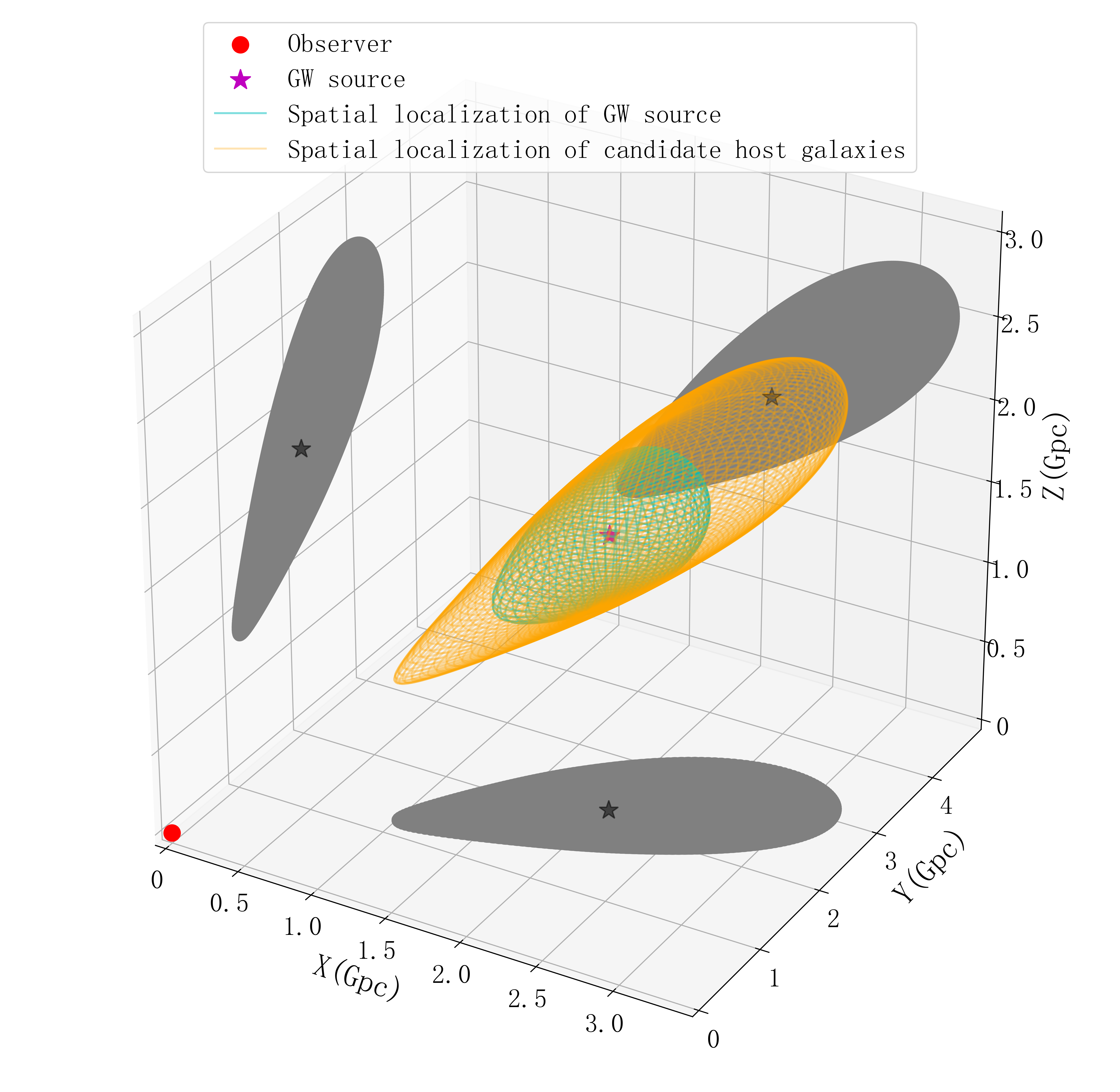
Figure 3: An example spatial localization error for a GW source. The cyan volume represents the spatial error due to the GW observation, while for the orange volume, we convert the $[z_{\min},z_{\max}]$ back into luminosity distance assuming the correct cosmology. The gray shadows are the projections of the spatial localization error, the red dot is the observer, and the purple star is the true input position of the GW source.

We then artificially assign a random galaxy to be the actual host galaxy. For a galaxy with bulge luminosity $L_{\rm bulge}$, we assign a weight according to a log-normal distribution with the $M_{\rm MBH}-L_{\rm bulge}$ relation. Next, we aim to simulate the real observation, to obtain a catalog of galaxies and to assign a probability of each galaxy hosting the merging black hole binary. Furthermore, we simulate the Malmquist bias to be more realistic. For the $j$th galaxy with luminosity $L_{j}$ and redshift $z_{j}$, the probability of it being recorded is

$${\rm erfc}(\log_{10}L_{j})=\frac{1}{\sqrt{2\pi\sigma_{\log_{10}L_{j}}}}\int_{\log_{10}L_{\rm limit}(z_{j},\vec{\Omega})}^{\infty}\exp\bigg{(}-\frac{1}{2}\frac{(\log_{10}L-\log_{10}L_{j})^{2}}{\sigma_{\log_{10}L_{j}}^{2}}\bigg{)}d(\log_{10}L)$$ (29)

where $\log_{10}L_{\rm limit}(z_{j},\vec{\Omega})=\frac{(+4.83-m_{\rm limit}-5)}{2.5}+2\log_{10}(\frac{D_{L}({z_{j},\vec{\Omega}})}{1\rm pc})$, dependent on a given set of cosmological parameters $\vec{\Omega}$, and we adopt a limiting magnitude of $m_{\rm limit}=+24\ \rm mag$ and equal measurement error of luminosity $\sigma_{\log_{10}L}=0.04$ (correspond to an uncertainty in magnitude of $0.1\ \textrm{mag}$) York:2000gk ; DES:2017myt ; Gong:2019yxt ; Laureijs:2011gra .

In the analysis stage, we try to eliminate the Malmquist bias by introducing a redshift-dependent correction factor using the luminosity function of both the galaxies MonteroDorta:2008ib ; Cohen:2001ag ; Marchesini:2006vg ; Faber:2005fp and the bulge. We need to manually augment sample sizes for further galaxies. We first divide the error box into multiple small regions both in sky location as well as in redshift. For each region, we can calculate the number of supplementary galaxies $\hat{N}_{\textrm{sup}}$ using a luminosity function $\Phi(L)$,

$$\hat{N}_{\textrm{sup}}=N_{\textrm{obs}}\frac{\int_{0}^{L_{\rm limit}}\Phi(L)dL}{\int_{L_{\rm limit}}^{\infty}\Phi(L)dL},$$ (30)

where we derive the luminosity function $\Phi(L)$ from the MDPL simulated catalog Conroy:2009gw . For a given GW source, the debiased prior of the location is determined by the possible host galaxies, which can be expressed as

$$p_{0}^{\textrm{debiased}}(z,\alpha,\delta,L_{\rm bulge}|\vec{\Omega},I)\simeq\frac{1}{N_{\rm tot}}\sum\bigg{(} \sum_{m=1}^{N_{\textrm{obs}}}\mathcal{N}(z|{\bar{z}^{m}},\sigma_{z}^{m})\delta(\alpha-\alpha^{m})\delta(\delta-\delta^{m})\mathcal{N}(L_{\rm bulge}|\bar{L}_{\rm bulge}^{m},\sigma_{L_{\rm bulge}}^{m})$$

$$+ \hat{N}_{\textrm{sup}}\mathcal{N}(z|{\bar{z}_{\rm obs}},\sigma_{z,{\rm obs}})\delta(\alpha-\bar{\alpha}_{\textrm{obs}})\delta(\delta-\bar{\delta}_{\textrm{obs}})\Phi^{\prime}(L_{\rm bulge})\bigg{)},$$ (31)

where $N_{\textrm{tot}}=\sum(N_{\textrm{obs}}+\hat{N}_{\textrm{sup}})$, and $\bar{z}_{\textrm{obs}}$, $\bar{\alpha}_{\textrm{obs}}$, and $\bar{\delta}_{\textrm{obs}}$ are the mean values of redshift, longitude and latitude for the observed galaxies in the small region. For nearby galaxies ($z<1$), we assume that spectroscopic redshift information is available and therefore the error can be neglected DESI:2016fyo . However, for further galaxies the redshift if more likely obtained through photometric measurement, which is assumed to be associated with an error $\Delta z=0.03(1+z)$ Ilbert:2013bf ; Dahlen:2013fea . Therefore, we adopt

$$\sigma_{z}(z)=\left\{\begin{array}[]{ll}0,&z<1;\\ 0.03(1+z),&z\geq 1.\end{array}\right.$$ (32)

The bulge luminosity function with an apostrophe, $\Phi^{\prime}(L_{\rm bulge})$, is defined as

$$\Phi^{\prime}(L_{\rm bulge})=\left\{\begin{array}[]{ll}\frac{\Phi(L_{\rm bulge})}{\int_{0}^{L_{\rm bulge}^{\min}}\Phi(L_{\rm bulge})dL_{\rm bulge}},&0\leq L_{\rm bulge}\leq L_{\rm bulge}^{\min};\\ \\ 0,&L_{\rm bulge}\geq L_{\rm bulge}^{\min};\end{array}\right.$$ (33)

where $L_{\rm bulge}^{\min}$ is the minimum bulge luminosity of observed galaxies in the small region, and we derive the bulge luminosity function $\Phi(L_{\rm bulge})$ from the MDPL simulated catalog. We remark that the second term in Eq. (III.4) does not represent a new batch of galaxies, but rather an adjustment to the weights of existing galaxies.

Next we assign different weights for galaxies with different positions and bulge luminosities. We consider the two following methods:

• (i) fiducial method: each galaxy in the spatial localisation error box of the GW source has equal weight regardless of its position and luminosity information;

• (ii) weighted method: the weight of a galaxy is the product of both its positional weight and bulge luminosity weight.

The positional weight is simply determined by the 3D space localisation from the GW parameter estimation. The luminosity-related weight, on the other hand, is more complicated. For an observed galaxy, the weight is assigned through a log-normal distribution, with the expected redshifted mass value being the mean value derived from the GW parameter estimation, and standard deviation $\sigma_{\log_{10}M}$. And for a manually supplemented galaxy, a further integration of this log-normal distribution over luminosity up to $L_{\rm bulge}^{\min}$ is needed. A detailed expression for both the positional weight and the luminosity-related weight for a given galaxy is provided in Appendix B.

The luminosity-related weight of galaxies can be affected by the intrinsic scatters of the $M_{\rm MBH}-L_{\rm bulge}$ relation as well as the uncertainties related to the measurements. We define $\sigma_{\log_{10}M}$ as the root sum squared of the intrinsic scatter of the relation between the central MBH mass and the galactic bulge luminosity $\sigma_{M-L}^{\textrm{int}}$, the measurement error on the total mass of GW sources $\sigma_{\log_{10}M}^{\rm GW}$, and the error related to the bulge luminosity $k_{c}\sigma_{\log_{10}L_{\rm bulge}}^{\rm EM}$. We adopt $\sigma_{\log_{10}M}^{\rm GW}\equiv 0.05$ as a conservative choice since the mass parameter can usually be accurately determined through GW observation. For the measurement error on the bulge luminosity, since we do not have complete information on the bulge luminosity distribution for high redshift galaxies, we adopt the galaxy luminosity error as a proxy through $\sigma_{\log_{10}L_{\rm bulge}}^{\rm EM}\simeq 5(1+z)\sigma_{\log_{10}L}=0.2(1+z)$.

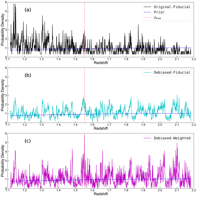
Figure 4: Example: Redshift distribution of galaxies for an example GW source. Top panel: Considering no debias correction, and assuming all galaxies within the error box as equally likely to be the host galaxy. Middle panel: Same as the top panel but including a correction for Malmquist bias. Bottom panel: Corrected for Malmquist bias, and assigning galaxy weights according to their position as well as luminosity. The vertical orange dashed line represents the real redshift of the GW event, and the horizontal blue dashed line represents the prior distribution where galaxies have constant density over comoving volume.

We demonstrate the effect of the debias and different weighting in Fig. 4. For the top panel, we do not correct for Malmquist bias, and there is an apparent excess of galaxies at low redshift. In the middle and bottom panel, the Malmquist bias is corrected by manually introducing supplementary galaxies; in these cases the distribution roughly follows the prior. For the top and middle panel, all galaxies within the error box are assumed equally likely to be the host galaxy of the MBHB merger, while for the bottom panel, we assign weights to the galaxies using the weighted method. One can observe that the bottom panel is less smooth, and the injected source stands out from the contaminating galaxies.

IV Cosmological Constraints

In this section, we explore quantitatively the prospects for parameter estimation with GW cosmology. We perform a series of Markov chain Monte Carlo (MCMC) studies using the widely adopted library emcee, a Python package that implements an affine-invariant MCMC ensemble sampler ForemanMackey:2012ig ; ForemanMackey:2019ig . For the detector(s), we consider various scenarios, including: TianQin, TianQin I+II, LISA, TianQin+LISA, and TianQin I+II+LISA. We investigate both the dark standard siren case, where no EM counterpart is available, and the bright standard siren case where we can use an EM counterpart to identify the host galaxy and therefore to obtain explicitly the redshift from EM observations. For the popIII and Q3d models we generate 200 mock GW events from MBHB mergers, while for the Q3nod model, the event rate of which is expected to be higher than the other two models, we generate 600 mock events. These events form three sample pools, and the GW events on which each realization of the cosmological parameter estimation relies are chosen randomly from these three pools.

In order to comprehensively probe the systematic and random errors in the inferred cosmological parameters, we repeat the cosmological analysis multiple times with independent runs for each detector configuration/MBHB population model/weighting method.

IV.1 TianQin and TianQin I+II

We first consider the most pessimistic scenario, where TianQin is operating alone and no EM counterpart is expected to be observed. For convenience, in this analysis we simply select all galaxies that fall into the range of $9\Delta\Omega\times[z_{\min},z_{\max}]$ (although the actual error box would correspond to a shape type characterised by Fig. 3).

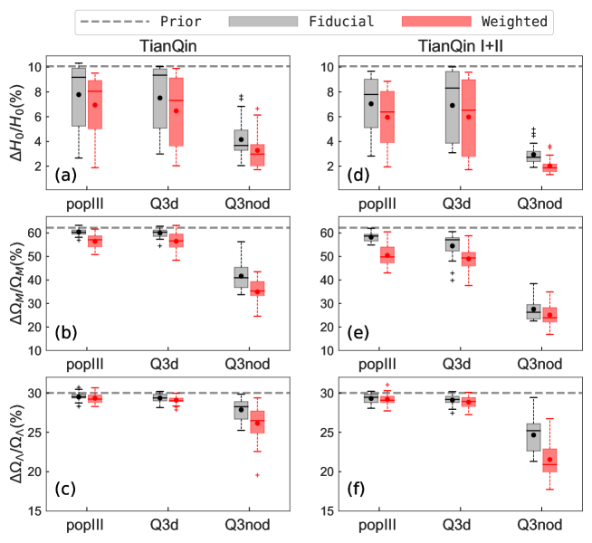
Figure 5: Boxplot of the precision of the estimated cosmological parameters for the three MBHB models, assuming two detector configurations, i.e., TianQin (left column) and TianQin I+II (right column). The top, middle, and bottom rows illustrate results for three cosmological parameters, $H_{0}$, $\Omega_{M}$, and $\Omega_{\Lambda}$, respectively. The horizontal gray dashed line represents a fiducial $68.27\%$ statistical interval from the prior. For each result, the box represents the range of $25\%-75\%$ of the data distribution, the upper limit of the whisker length is 1.5 times the box length, and the crosses are outliers. In each box, the dot represents the mean value, the short horizontal line represents the median value, using the fiducial method (gray) and the weighted method (red), respectively.

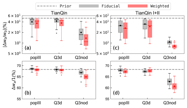
Figure 6: Boxplot of the precision of the estimated dark energy EoS parameters for the three MBHB models, assuming two detector configurations, i.e., TianQin (left column) and TianQin I+II (right column), and keeping non-CPL parameters fixed. The top and bottom illustrate results for three cosmological parameters, $w_{0}$ and $w_{a}$, respectively. The horizontal gray dashed line represents a fiducial $68.27\%$ statistical interval from the prior. The gray and red boxplots represent the distribution of estimation precisions of the parameters using the fiducial method and the weighted method, respectively.

As illustrated by 2019PhRvD..99l3002F , the SNR accumulates rather quickly just before the final merger. Therefore, the difference in the precision of cosmological parameter estimation between TianQin and TianQin I+II is rooted in their different detection numbers. The distributions of the constraint precisions of various cosmological parameters for TianQin (left column) and TianQin I+II (right column) under the three MBHB population models are shown in Fig. 5. In order to eliminate the random fluctuations caused by the specific choice of any event, we repeat this process 24 times, and the constraint results are presented in the form of boxplots.

The top, middle, and bottom rows represent the estimation precision of $H_{0}$, $\Omega_{M}$, and $\Omega_{\Lambda}$, respectively. The constraining ability of these parameters are decreasing as with this order. In each panel, from left to right, we show the results adopting popIII, Q3d, and Q3nod as the underlying astrophysical model, respectively. In each model, we generate a number of GW event catalogs, assuming an event rate that follows a Poisson distribution with the rate parameter determined by Table I. It can be observed that more events leads to better constraints on the cosmological parameters. Furthermore, the weighted method (red box) shows better constraining ability than the fiducial method (gray box).

In general, under the models with a lower MBHB event rate, such as popIII and Q3d models, we can only constrain the Hubble constant, which is almost entirely determined by low redshift GW events. The constraints of other cosmological parameters require more GW events, which is feasible under the Q3nod model. For TianQin, the relative precision on $H_{0}$ is estimated to be $7.8\%$, $7.5\%$ and $4.2\%$ via the fiducial method; by using the weighted method, the relative precision can reach $6.9\%$, $6.5\%$ and $3.3\%$, for the popIII, Q3d and Q3nod models, respectively. For TianQin I+II, the number of MBHB mergers would be boosted by a factor of about 2, and the relative error of $H_{0}$ reduces to $6.0\%$, $6.0\%$, and $2.0\%$ using the weighted method, respectively. Under the Q3nod model, $\Omega_{M}$ and $\Omega_{\Lambda}$ are expected to be constrained to a relative precision of $34.9\%$ ($25.1\%$) and $26.1\%$ ($21.5\%$) for TianQin (TianQin I+II), respectively.

Finally, we study the constraining power of the GW observations on the EoS of dark energy, assuming the CPL model for its redshift evolution. Here we fix $H_{0}=67.8$ km/s/Mpc, $\Omega_{M}=0.307$, and $\Omega_{\Lambda}=0.693$. We find that, for all astrophysical models and detector configurations, $w_{a}$ can hardly be constrained; however, meaningful constraints can be obtained on $w_{0}$, as shown in Fig. 6. And similarly, the weighted method also leads to more precise constraints on the parameters of EoS of dark energy compared to the fiducial method. If using the weighted method, the relative precision of $w_{0}$ can be reach a level of $36.7\%$, $37.2\%$, and $13.8\%$ for TianQin, and $26.6\%$, $29.6\%$, and $8.1\%$ for TianQin I+II — for popIII, Q3d, and Q3nod models respectively.

Besides, in order to more graphically represent the advantages of the weighted method over the fiducial method, we show in Appendix C, the typical posterior probability distributions of the cosmological parameters and the parameters of EoS of the dark energy constrained by TianQin.

IV.2 Network of TianQin and LISA

For GW observations, the power of the cosmological constraints is crucially related to how well the sky positions of the sources may be determined. With a network of multiple GW detectors working simultaneously, one can greatly improve this sky localisation error. The orbital planes of the TianQin constellation and LISA constellation are pointing in different directions; thus, joint detections can break the degeneracy between longitude and latitude of GW source, and the difference in the arrival time between the two detectors can also narrow the margin of the localisation error. However, the measurement of $D_{L}$ suffers from the systematics arising from weak lensing and peculiar velocities, and thus can hardly be improved even in the network observation case.

In what follows, we consider the cosmological constraints from a network of TianQin and LISA. As shown in Figs. 7 and 8, compared with the TianQin alone scenario, the network of TianQin and LISA can consistently improve the constraints on the cosmological parameters. This improvement benefits from both the increased detection numbers with more detectors (as illustrated in Table I) and the better localisation capability of the network (as illustrated in Fig. 2).

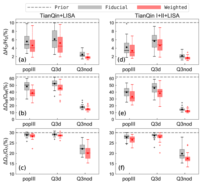
Figure 7: Same as Fig. 5, but for TianQin+LISA (left column) and TianQin I+II+LISA (right column), respectively.

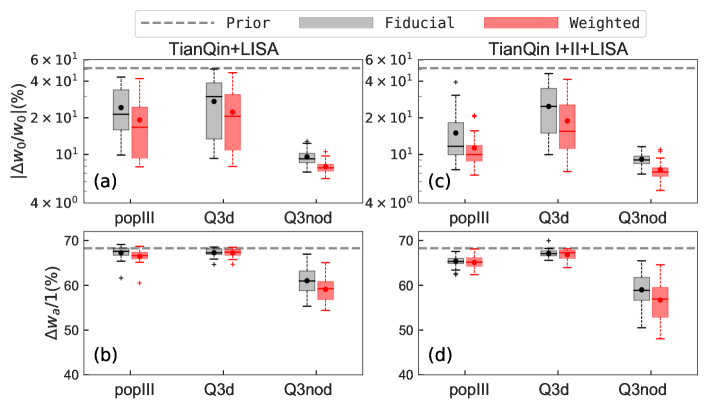
Figure 8: Same as Fig. 6, but for TianQin+LISA (left column) and TianQin I+II+LISA (right column), respectively.

Figure 7 illustrates how the relative precision of constrained cosmological parameters corresponding to different detector network configurations, MBHB population models, and weighting methods, with a similar setup as in Fig. 5. Comparing these two figures, it is easy to see that the joint detections can effectively improve the constraint precision on the Hubble constant $H_{0}$. Similarly, the fractional dark energy density $\Omega_{\Lambda}$ is still poorly constrained, except under the Q3nod model. However, different from the TianQin alone case, here we can obtain a meaningful constraints on the fractional total matter density $\Omega_{M}$ in all cases. Again, compared with the fiducial method, the weighted method can significantly reduce the uncertainties on the Hubble constant.

In particular, using the weighted method, TianQin+LISA GW detections lead to a precision of $4.7\%$, $5.2\%$, and $1.8\%$ on measurements of $H_{0}$ for the popIII, Q3d, and Q3nod models, respectively; while the TianQin I+II+LISA detections further improve the precision of $H_{0}$ measurements to $3.4\%$, $4.7\%$, and $1.7\%$, respectively for these three astrophysical models. These kinds of measurements would be interesting, since they could be helpful for resolving (or confirming) the Hubble tension Freedman:2017yms ; Verde:2019ivm ; Aghanim:2018eyx ; Riess:2020sih ; Riess:2020fzl .

When assuming a dynamical dark energy model, the joint detection of TianQin and LISA can improve the constraints on $w_{0}$ (see Fig. 8), while $w_{a}$ is still poorly constrained. With the weighted method scheme, for TianQin+LISA, $w_{0}$ can be constrained to a level of $19.2\%$, $22.3\%$ and $7.9\%$ in popIII, Q3d and Q3nod model, respectively; assuming a joint detection of TianQin I+II+LISA, one can better constrain the dark energy EoS parameters, $w_{0}$ can be constrained to a level of $11.3\%$, $18.9\%$ and $7.5\%$, respectively. Especially, in the case of adopting the Q3nod model, the constraint precisions on the parameters of EoS of dark energy become comparable to those from current EM observations Aghanim:2018eyx ; Abbott:2018wzc . Thus, the GW observations can provide an independent verification of our current understanding of the Universe Freedman:2017yms ; Riess:2020sih ; Riess:2020fzl ; Benevento:2020fev ; Alestas:2020mvb ; DiValentino:2017iww ; Cai:2021wgv .

Table II: Expected relative precision on ($H_{0}$, $\Omega_{M}$, $\Omega_{\Lambda}$) and ($w_{0}$, $w_{a}$) constraints for the three MBHB models, assuming different configurations of detectors or networks. When constraining $H_{0}$, $\Omega_{M}$, and $\Omega_{\Lambda}$, no evolution of dark energy is assumed, while all other cosmological parameters are fixed when studying the CPL parameters. Numbers are shown for mean values (median values in brackets). The symbol “$-$” indicates that the corresponding parameter is not effectively constrained under the corresponding condition.

Cosmological	Detector	Expected relative precision(%)
		popIII		Q3d		Q3nod
parameter	configuration	Fiducial	Weighted	Fiducial	Weighted	Fiducial	Weighted
	TianQin	$7.8$ (9.2)	$6.9$ (8.1)	$7.5$ (9.4)	$6.5$ (7.3)	$4.2$ (3.7)	$3.3$ (3.0)
	TianQin I+II	$7.0$ (7.8)	$6.0$ (6.4)	$6.9$ (8.3)	$6.0$ (6.5)	$2.9$ (2.7)	$2.0$ (1.9)
$\Delta H_{0}/H_{0}$	LISA	$7.2$ (7.2)	$5.6$ (5.8)	$7.7$ (8.2)	$6.8$ (7.8)	$2.8$ (2.9)	$2.1$ (1.9)
	TianQin+LISA	$5.6$ (4.8)	$4.7$ (4.1)	$6.1$ (5.8)	$5.2$ (4.5)	$2.5$ (2.3)	$1.8$ (1.8)
	TianQin I+II+LISA	$4.2$ (3.5)	$3.4$ (3.0)	$5.7$ (5.9)	$4.7$ (4.8)	$2.2$ (2.0)	$1.7$ (1.7)
	TianQin	$-$	$56.5$ (57.1)	$-$	$56.5$ (56.6)	$41.6$ (40.9)	$34.9$ (35.3)
	TianQin I+II	$58.2$ (58.7)	$50.5$ (49.8)	$54.5$ (57.1)	$49.0$ (49.4)	$28.1$ (27.7)	$25.1$ (23.9)
$\Delta\Omega_{M}/\Omega_{M}$	LISA	$56.2$ (56.5)	$49.6$ (49.8)	$55.4$ (55.7)	$49.7$ (49.9)	$21.7$ (20.0)	$17.5$ (16.4)
	TianQin+LISA	$48.3$ (50.4)	$38.7$ (38.3)	$52.5$ (52.8)	$45.8$ (45.2)	$18.3$ (17.9)	$15.2$ (14.6)
	TianQin I+II+LISA	$40.0$ (40.4)	$33.4$ (31.4)	$46.0$ (47.7)	$38.5$ (41.2)	$14.8$ (13.9)	$12.4$ (11.8)
	TianQin	$-$	$-$	$-$	$-$	$27.9$ (28.3)	$26.1$ (26.5)
	TianQin I+II	$-$	$-$	$-$	$-$	$24.6$ (25.0)	$21.5$ (20.9)
$\Delta\Omega_{\Lambda}/\Omega_{\Lambda}$	LISA	$-$	$-$	$-$	$-$	$23.6$ (24.2)	$21.5$ (22.5)
	TianQin+LISA	$-$	$-$	$-$	$-$	$22.2$ (22.3)	$20.1$ (20.2)
	TianQin I+II+LISA	$-$	$26.6$ (27.1)	$-$	$-$	$19.9$ (18.9)	$17.6$ (17.2)
	TianQin	$40.3$ (46.1)	$36.7$ (41.7)	$42.4$ (47.4)	$37.2$ (45.1)	$20.0$ (17.3)	$13.8$ (10.9)
	TianQin I+II	$31.6$ (31.1)	$26.6$ (26.1)	$34.7$ (34.5)	$29.6$ (31.5)	$10.5$ (9.8)	$8.1$ (7.6)
$|\Delta w_{0}/w_{0}|$	LISA	$35.1$ (35.6)	$23.7$ (23.8)	$36.0$ (41.0)	$29.7$ (33.7)	$11.4$ (11.0)	$8.1$ (7.9)
	TianQin+LISA	$24.3$ (21.4)	$19.2$ (16.7)	$27.3$ (29.9)	$22.3$ (20.6)	$9.6$ (9.2)	$7.9$ (7.8)
	TianQin I+II+LISA	$15.0$ (11.7)	$11.3$ (10.0)	$24.8$ (24.9)	$18.9$ (15.5)	$9.1$ (9.0)	$7.5$ (7.2)
	TianQin	$-$	$-$	$-$	$-$	$-$	$-$
	TianQin I+II	$-$	$-$	$-$	$-$	$62.8$ (63.0)	$60.7$ (60.4)
$\Delta w_{a}/1$	LISA	$-$	$-$	$-$	$-$	$62.8$ (62.8)	$60.0$ (59.1)
	TianQin+LISA	$-$	$-$	$-$	$-$	$61.0$ (61.0)	$59.1$ (59.2)
	TianQin I+II+LISA	$-$	$-$	$-$	$-$	$59.0$ (58.9)	$56.7$ (56.9)

Table II summarises the relative precision on $H_{0}$, $\Omega_{M}$, and $\Omega_{\Lambda}$, as well as $w_{0}$ and $w_{a}$, under various detection scenarios. Each result is obtained by marginalizing over the other parameters, while all three parameters of $\Lambda$CDM model are fixed when constraining $w_{0}$ and $w_{a}$. In order to mitigate the impact of random errors, we independently generate 24 GW event catalogs for each detector configuration/MBHB population model/weighting method, and present the mean values and median values of the relative constraint precisions of these five parameters. This table shows that the positional and bulge luminosity weighting of the host galaxies is very helpful for improving the precision of the parameter estimation. And a network of TianQin and LISA yield better constraints than both TianQin and LISA. In the most ideal scenario, $H_{0}$, $\Omega_{M}$, and $\Omega_{\Lambda}$ can be estimated with a relative precision of $1.7\%$, $12.4\%$, and $17.6\%$, while $w_{0}$ and $w_{a}$ can be constrained to $7.5\%$ and $56.7\%$, respectively.

IV.3 EM-bright scenario

Some literature has suggested that MBHB mergers can be accompanied by x-ray, optical, or radio activity Dotti:2011um ; 2016JCAP…04..002T , although it is not yet certain about the physical properties of the EM counterpart for GW events. In most cases, the gas-rich environment near the MBHBs is considered to be responsible for such EM transients. For example, in the late stage of binary evolution, the gas within the binary orbit would be driven inward by the inspiralling MBHB. The accretion rate can exceed the Eddington limit, forming high-velocity outflows and emitting strong EM radiation Armitage:2002uu . If the component MBHs are highly spinning with aligned spin, the external disk can extract energy from the orbiting MBHB until merged, forming dual jets and observable emissions in a way similar to the Blandford-Znajek mechanismPalenzuela:2010nf . General relativistic magnetohydrodynamic simulations of magnetized plasma show that MBHBs can amplify magnetic fields by strong accretion and emit strong EM signals Giacomazzo:2012iv . Some have argued that jets are increasingly dominated by magnetic fields, and can lead to transient emission after the merger Gold:PRD2014 . Hydrodynamic simulations including viscosity indicate that, before merger, the MBHB will transfer orbital energy into internal shocks and emit through x-ray radiation Farris:mnrasl2014 .

In view of these literatures, it is interesting to consider the optimistic scenario, where an EM counterpart of each MBHB merger is identified, and these counterparts are further used to extract redshift information from the host galaxy observation 2016JCAP…04..002T . This possibility would be enhanced by a number of current or planned EM facilities with large field of view and high sensitivity, including Einstein Probe EinsteinProbeTeam:2015bcj ; Liu:2020bgc , Chinese Space Station Telescope (CSST) Gong:2019yxt , Euclid telescope Laureijs:2011gra , Vera Rubin Observatory Ivezic:2008fe , Five-hundred-meter Aperture Spherical radio Telescope (FAST) Jiang:2019rnj , and Square Kilometre Array (SKA) Feng:2020nyw . We remark also that this bright standard siren analysis can serve as a lower limit for the precision of cosmological parameter estimation in the dark standard siren scenario — at least in the absence of any additional mitigating strategy to deal with the impact of weak lensing and/or peculiar velocity errors. In our bright standard siren analysis, we apply the same selection criteria as 2016JCAP…04..002T , and only consider the GW events with $\rho\geqslant 8$ and $\Delta\Omega\leqslant 10\ \textrm{deg}^{2}$ (and $z<3$, additionally).

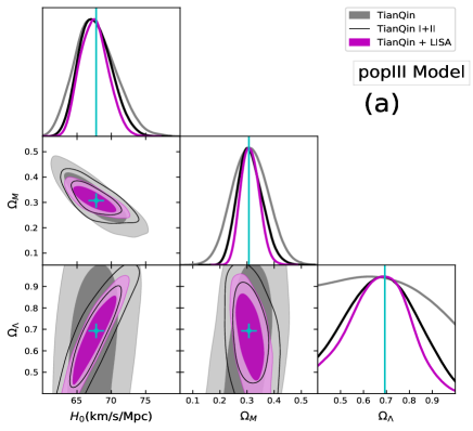
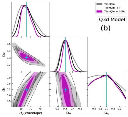
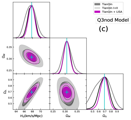
Figure 9: Typical results for the estimation of cosmological parameters under the optimistic scenario with an explicit EM counterpart. Contours show the $68.27\%$ and $95.45\%$ confidence levels, assuming different detector configurations of TianQin (grey shadow), TianQin I+II (black line), and TianQin+LISA (magenta shade), respectively. The three subplots correspond to adopting popIII, Q3d, and Q3nod respectively as the underlying model for MBHB mergers.

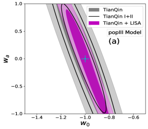
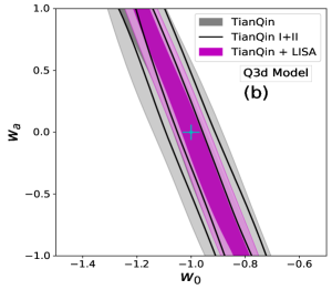
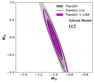
Figure 10: Typical results for the estimation of dark energy EoS parameters under the optimistic scenario with an explicit EM counterpart. Contours show the $68.27\%$ and $95.45\%$ confidence levels, assuming different detector configurations of TianQin (grey shadow), TianQin I+II (black line), and TianQin+LISA (magenta shade), respectively. The three subplots correspond to adopting popIII, Q3d, and Q3nod respectively as the underlying model for MBHB mergers. The other cosmological parameters, $H_{0}$, $\Omega_{M}$, and $\Omega_{\Lambda}$ are fixed.

In Fig. 9, we illustrate the expected probability distribution of $(H_{0},\Omega_{M},\Omega_{\Lambda})$, while in Fig. 10 we show the expected results for the CPL parameters $(w_{0},w_{a})$. In both cases, we consider three detector configurations, namely TianQin, TianQin I+II, and TianQin+LISA, represented by the grey shadow, black line, and magenta shades, respectively. We also consider the popIII, Q3d, and Q3nod models. Correspondingly, the marginalised one dimensional relative errors of the parameters for various detector configuration are listed in Table III.

Table III: Constraints on the cosmological parameters and dark energy EoS parameters under the optimistic scenario that an EM counterpart is observed, considering different detector configurations and underlying MBHB merger models. Notice that the cosmological parameters ($H_{0}$, $\Omega_{M}$, $\Omega_{\Lambda}$) and CPL parameters $(w_{0},\ w_{a})$ are studied separately. Each result is obtained based on 108 replicated and independent random realizations, the error represents $68.3\%$ confidence interval.

		Relative error(%)
Cosmological parameter	Population model	TianQin	TianQin I+II	LISA	TianQin+LISA	TianQin I+II+LISA
	popIII	$4.3_{-2.0}^{+3.0}$	$3.4_{-1.3}^{+1.9}$	$3.9_{-1.4}^{+2.8}$	$3.1_{-1.0}^{+1.3}$	$2.5_{-0.7}^{+1.5}$
$\Delta{H_{0}}/H_{0}$	Q3d	$6.2_{-3.4}^{+2.2}$	$4.5_{-2.4}^{+2.2}$	$4.9_{-2.3}^{+2.0}$	$3.8_{-1.7}^{+3.0}$	$3.6_{-1.5}^{+2.7}$
	Q3nod	$1.9_{-0.5}^{+0.7}$	$1.4_{-0.2}^{+0.3}$	$1.4_{-0.3}^{+0.5}$	$1.3_{-0.2}^{+0.4}$	$1.2_{-0.2}^{+0.3}$
	popIII	$19.9_{-6.7}^{+11.9}$	$13.1_{-3.3}^{+7.8}$	$14.8_{-3.8}^{+10.2}$	$9.9_{-1.9}^{+4.5}$	$7.9_{-1.2}^{+4.5}$
$\Delta{\Omega_{M}}/\Omega_{M}$	Q3d	$27.3_{-11.9}^{+8.8}$	$16.3_{-5.5}^{+9.6}$	$19.6_{-7.1}^{+9.3}$	$14.6_{-4.7}^{+10.1}$	$12.9_{-3.5}^{+9.3}$
	Q3nod	$6.5_{-0.7}^{+1.3}$	$4.7_{-0.4}^{+0.6}$	$5.0_{-0.4}^{+0.8}$	$4.4_{-0.4}^{+0.7}$	$3.9_{-0.3}^{+0.7}$
	popIII	$27.7_{-2.8}^{+0.8}$	$25.0_{-4.1}^{+2.9}$	$26.5_{-3.6}^{+1.4}$	$21.8_{-3.0}^{+4.1}$	$20.2_{-4.1}^{+4.1}$
$\Delta{\Omega_{\Lambda}}/\Omega_{\Lambda}$	Q3d	$27.8_{-1.4}^{+0.9}$	$27.0_{-6.2}^{+1.1}$	$27.4_{-4.3}^{+1.0}$	$25.6_{-6.4}^{+2.3}$	$24.9_{-6.5}^{+2.4}$
	Q3nod	$16.0_{-2.4}^{+3.5}$	$11.3_{-1.3}^{+1.8}$	$12.3_{-1.7}^{+3.0}$	$10.7_{-0.9}^{+2.0}$	$9.5_{-1.0}^{+1.5}$
	popIII	$11.6_{-1.9}^{+4.2}$	$10.6_{-1.8}^{+2.5}$	$11.4_{-2.0}^{+3.2}$	$9.8_{-1.5}^{+2.5}$	$9.4_{-1.6}^{+1.9}$
$|\Delta{w_{0}}/w_{0}|$	Q3d	$13.8_{-3.3}^{+2.9}$	$12.3_{-2.4}^{+2.0}$	$13.1_{-2.3}^{+2.2}$	$12.2_{-2.4}^{+2.2}$	$11.2_{-1.7}^{+2.6}$
	Q3nod	$8.5_{-1.3}^{+1.7}$	$6.7_{-0.6}^{+1.1}$	$6.8_{-0.9}^{+1.5}$	$6.6_{-0.9}^{+1.0}$	$5.7_{-0.8}^{+1.1}$
	popIII	$66.1_{-3.8}^{+2.0}$	$61.7_{-3.5}^{+4.0}$	$64.0_{-4.5}^{+2.9}$	$57.8_{-4.9}^{+5.7}$	$53.5_{-3.9}^{+6.0}$
$\Delta{w_{a}}/1$	Q3d	$67.0_{-3.9}^{+1.1}$	$64.9_{-4.2}^{+2.4}$	$66.3_{-4.4}^{+1.2}$	$63.7_{-5.7}^{+3.2}$	$62.6_{-4.9}^{+3.5}$
	Q3nod	$49.3_{-3.9}^{+5.3}$	$39.0_{-2.8}^{+5.2}$	$40.8_{-3.2}^{+5.4}$	$37.3_{-3.9}^{+4.2}$	$33.0_{-2.7}^{+4.0}$

As expected, with the identified EM counterparts, one can significantly improve the ability of the standard sirens to constrain the cosmological parameters. For TianQin, the relative precision of $H_{0}$ can be as small as $1.9\%$, which translates into an absolute precision of about $\Delta H_{0}=1.3~{}\rm{km/s/Mpc}$. For TianQin I+II, the relative precision of $H_{0}$ can be as small as $1.4\%$, which exceeds the constraint accuracy for TianQin+LISA in the dark standard siren scenario. If TianQin I+II+LISA is implemented, the relative precision of $H_{0}$ can be as small as $1.2\%$, which translates into an absolute precision of about $\Delta H_{0}=0.8~{}\rm km/s/Mpc$. Furthermore, the fractional density parameter $\Omega_{\Lambda}$ and the EoS parameter $w_{a}$ for the dark energy, which in the dark standard siren scenario are hardly constrained, can also be constrained to a relative precision of as small as $9.5\%$ and $33.0\%$ when the EM counterpart available. These constraints are comparable to those from analysis of other cosmological EM survey data Abbott:2018wzc ; Abdullah:2020qmm .

V Discussion

V.1 Constraining ability from different redshifts

For a given GW event, its ability to constrain the cosmological parameters depends on two factors: its spatial localization accuracy, and the cosmological evolution between the source and the observer.

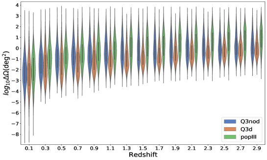
Figure 11: Distribution of TianQin localization areas. Each violin plot stacks 1000 GW events around the given redshifts $[(z-0.1),(z+0.1)]$.

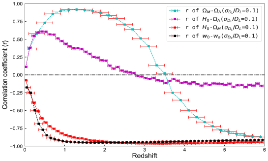
Figure 12: Evolution of the correlation coefficient (indicated by $r$) with redshift. For a given redshift bin of width 0.05/0.1/0.2, we randomly generate a number of EM-bright standard sirens, obtain the MCMC samples and compute correlation coefficients on $H_{0}-\Omega_{M}$/$H_{0}-\Omega_{\Lambda}$/$\Omega_{M}-\Omega_{\Lambda}$/$w_{0}-w_{a}$, respectively. Due to the large uncertainties for some parameters, we choose a slightly different prior for $h\in\textrm{U}[0.4,1]$, $\Omega_{M}\in\textrm{U}[0,0.6]$, $\Omega_{\Lambda}\in\textrm{U}[0.4,1]$, and $w_{0}\in\textrm{U}[-2.5,0.5]$, $w_{a}\in\textrm{U}[-3,3]$.

In Fig. 11, we show the distribution of sky localization errors for MBHBs mergers at different redshifts. We see the sky localization area $\Delta\Omega$ tends to increase as the redshift increases. Meanwhile, nearby events are usually accompanied by larger SNR, which leads to better determination of the luminosity distance. To sum up, for nearby events, the smaller localization area together with the better distance estimation leads to a smaller error box, and therefore a smaller number of candidate host galaxies.

On the other hand, given the same $\Delta D_{L}$ and $\Delta\Omega$, the GW signals at different redshifts lead to different constraints on the cosmological parameters. In Fig. 12, we illustrate the degeneracy of the cosmological parameters by showing the evolution of correlation coefficients between different pairs of parameters. To do this, we estimate cosmological parameters with a sample of EM-bright GW events, assuming a relative error on luminosity distance $\sigma_{D_{L}}/D_{L}=0.1$.

We find that, the $H_{0}$ constraint from high redshifts suffers from strong degeneracy with $\Omega_{M}$ and $\Omega_{\Lambda}$, and this degeneracy becomes less significant only at very low redshifts. Notice that the correlation coefficient between $\Omega_{M}$ and $\Omega_{\Lambda}$ switches its sign at $z\sim 3.5$, suggesting that observations of both higher and lower redshift events are needed to alleviate the degeneracy. Also, the correlation coefficient between $w_{0}$ and $w_{a}$ is approaching total anticorrelation at $z\gtrsim 1$. These two parameters cannot be precisely measured, partly because of the strong anticorrelation between them.

In conclusion, a small number of low redshift GW sources is sufficient to provide a good constraint on the $H_{0}$, thanks to the precise position estimation, as well as the weaker parameter degeneracies. Meanwhile, high redshift events are useful to better constrain other cosmological parameters like $\Omega_{M}$ and $\Omega_{\Lambda}$. For cases where the EM counterpart can be uniquely identified, the GW events with large redshift can give tight constraints on the cosmological parameters; otherwise the large positional error would weaken such constraints.

V.2 Effects of redshift limit

Throughout this study we have applied a cutoff for events beyond redshift $z=3$. To some extent, this cutoff reflects the incompleteness of galaxy catalogs at higher redshifts. It is very challenging to pursue relatively complete galaxy catalog at high redshift. Such as, sky surveys like the Sloan Digital Sky Survey (SDSS) Alam:2015mbd ; Abolfathi:2017vfu ; SDSS-IV:2019txh and Dark Energy Survey (DES) DES:2017myt can reliably map galaxies as far as $z\simeq 1.2$.

Our paper highlights the need for more detailed galaxy surveys with redshift limit of $z>3$. Actually, it is not beyond the imagination that, once MBHB mergers are routinely detected, intensive observations would be triggered to map the higher redshift Universe — at least within the sky localization regions of the observed mergers — and thus provide a more complete catalog of galaxies therein 2015ApJ…801L…1B .

Moreover, the redshift limit for quasar observations is much larger than that for galaxies. For example, the redshift limit of the quasar catalog mapped by SDSS can reach $z\simeq 4$ Abolfathi:2017vfu ; SDSS-IV:2019txh . Meanwhile, some have argued that quasars can host the MBHBs Sobacchi:2016yez ; Connor:2019gun ; Penil:2020uqg . In addition to the quasars, one can also explore the potential of using Lyman-$\alpha$ forest effect to obtain redshift information Hess:2018qit ; Ravoux:2020bpg ; Qin:2021gkn ; Porqueres:2019dpn . It is still possible to obtain statistical redshift for the high-redshift GW sources.

V.3 Importance of bulge luminosity information

Throughout this paper, we have incorporated both position and bulge luminosity information for the calculation of weights that we assign to candidate host galaxies. Here we demonstrate the importance of the bulge luminosity alone, by weighting only on spatial location information. As shown in Fig. 13, compared with the fiducial method, the relative error on $H_{0}$ shrinks when sky location information is included, but the bulge luminosity weight consistently improves the estimation precision. For mergers with higher redshift, the importance of the bulge luminosity is weakened, due to the large localization error volume and the incompleteness of the galaxy catalog. The large number of galaxies within this volume, combined with large uncertainty associated with the bulge luminosity, decreases the effectiveness of the weighting scheme. On the other hand, the galaxy catalog is incomplete at high redshift, and the introduction of the luminosity function and the bulge luminosity function only compensates the weights of high redshift bright galaxies to some extent [see Eqs. (30) and (III.4)], which does not help to weight the “correct” host galaxies for the high redshift GW sources with lower mass.

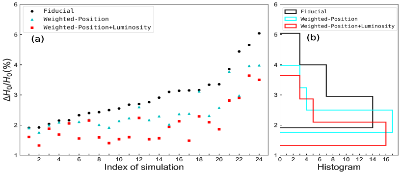
Figure 13: Comparison of the relative errors on the Hubble constant $H_{0}$ under different weighting methods, assuming GW detections with TianQin I+II under the Q3nod MBHB model and no EM counterpart. Left panel: Each point represents the relative error on $H_{0}$ for an individual simulation corresponding to the fiducial (black dot), the position-only weighted (cyan triangle), and the position+luminosity weighted (red square) method, respectively. Right panel: Histogram of the relative error on $H_{0}$ for the three different weighting methods.

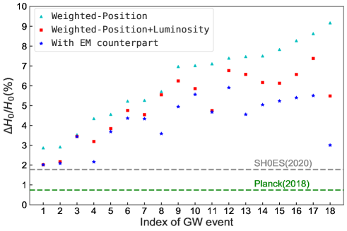
Figure 14: Comparison of the constraints on the Hubble constant $H_{0}$ by an individual nearby event for the following scenarios: with EM counterpart (blue star), using the position+luminosity weighted method (red square), and using position-only weighted method (cyan triangle). Each index represents one nearby GW event. The green line represents the $H_{0}$ error measured by $Planck$ using CMB anisotropies Aghanim:2018eyx , and the gray line represents the $H_{0}$ error measured by the SH0ES project using type Ia supernovae data Riess:2020fzl . These events are selected from the sample pool of the Q3nod model with the conditions of both $z\lesssim 0.5$ and $\Delta\Omega\lesssim 5\times 10^{-3}{\rm deg}^{2}$.

However, the bulge luminosity weight plays a crucial role especially when nearby events are considered, since only a relatively small number of galaxies is located within the error box. In this case, therefore one host galaxy can be largely identified through the $M_{\rm MBH}-L_{\rm bulge}$ relation. Fig. 14 illustrates the constraints on the Hubble constant for the nearby events with both $z\lesssim 0.5$ and $\Delta\Omega\lesssim 5\times 10^{-3}~{}{\rm deg}^{2}$ in three scenarios, i.e., with EM counterpart, using the position plus luminosity weighted method, and using position-only weighted method. We can observe that, by using the $M_{\rm MBH}-L_{\rm bulge}$ relation, the constraint precision on the Hubble constant in the dark siren scenario can be greatly improved, sometimes even comparable to scenarios with EM counterpart. Since we also expect that it would be easier to obtain more complete information on the bulge luminosity for nearby galaxies, this fact highlights the importance and potential efficacy of the bulge luminosity information.

V.4 Scope of the $M_{\rm MBH}-L_{\rm bulge}$ relation and the luminosity function

We have demonstrated that performing a weighting process of candidate host galaxies according to the $M_{\rm MBH}-L_{\rm bulge}$ relation is vital to improve the precision of the measured cosmological parameters. In this paper, a default assumption is adopted in our calculation, which is that the $M_{\rm MBH}-L_{\rm bulge}$ relation applies to all MBHBs independent of the mass of the GW source. This relation behaves differently at the low-mass end than at the high-mass end Jiang:2011bt ; Kormendy:2013dxa , and we have used different values of intrinsic scatter at the high and low-mass ends, see Eq. (28). In this part we discuss the scope of application of this relation.

For TianQin, the MBHB events with $M>5\times 10^{6}M_{\odot}$ account for about $18\%$, $16\%$ and $21\%$ of the total detectable events under popIII, Q3d and Q3nod models, respectively; for LISA, these percentages are about $44\%$, $36\%$ and $40\%$, respectively. The high-mass MBHB GW sources account for quite a large proportion of the total detectable events. For the low-mass MBHs with $M<10^{6}M_{\odot}$, their host galaxies show no co-evolution with the central MBHs Jiang:2011bt ; Jiang:2011bu . The low-mass MBHs are more likely to be remnants of black hole seeds, for a given MBH mass, the possible bulge luminosity spans a larger range Jiang:2011bt .

Bulges at the centers of galaxies can be classified as either classical bulges or pseudo-bulges, depending on whether they contain disk structures (pseudo-bulges) or not (classical bulges). Based on numerical simulations of galaxy collisions, it is generally accepted that classical bulges are made in major mergers of galaxies, whereas pseudobulges are the result of internal evolution of galaxy disks since their formation Kormendy:2013dxa . It is noteworthy that the host galaxies of the low-mass MBHs that deviate from the $M_{\rm MBH}-L_{\rm bulge}$ relation almost all have pseudobulges in their centers Jiang:2011bt . This implies that the deviations from the $M_{\rm MBH}-L_{\rm bulge}$ relation at the low-mass end do not unduly affect the scope of the weighted method proposed in this paper, and it is sufficient to account for this effect by adopting a larger intrinsic scatter, see Eq. (28).

In addition to the bulge luminosity information of galaxies, other observable information about galaxies such as stellar velocity dispersion and galaxy morphology may provide additional constraints on MBH mass for the lighter ones. The relation between MBH mass and stellar velocity dispersion (the $M_{\rm MBH}-\sigma$ relation) at the low-mass end is consistent with that at the high-mass end Xiao:2011xg . Even such information is not available a prior, telescopes would be motivated to perform deep observations after the GW detection, especially when the sky location can be very precisely determined.

We also examine other aspects of this relation. Throughout this paper we have assumed a universal $M_{\rm MBH}-L_{\rm bulge}$ relation, obtained from fitting the observed data at $z\approx 0$ Bentz:2008rt ; Kormendy:2013dxa . However, due to the lack of reliable models, we ignore the possible redshift evolution of this $M_{\rm MBH}-L_{\rm bulge}$ relation, which might cause some bias in our analysis. In the weighting process, we choose a moderately large $\sigma_{\log_{10}M}$ so that such bias can be partially absorbed.

Another possible source of bias is introduced by ignoring the redshift evolution of the luminosity function. We manually augmented our galaxy samples, according to the modelled luminosity function, to remove the Malmquist bias. However, the luminosity function is only complete for nearby redshifts, and becomes more and more incomplete as the redshift increases Marchesini:2006vg ; Faber:2005fp ; Shen:2020obl . We therefore highlight also the need for a more thorough and precise luminosity function evolution model, which can be obtained by existing McLure:2012fk ; Bouwens:2014fua and future ultradeep-field observations Gong:2019yxt ; Laureijs:2011gra .

Notice that most galaxy catalogs constructed from cosmological surveys do not list the galactic bulge luminosity of each source. In order to use bulge luminosity to improve our weighting scheme, we need to extract this information from data. Since the luminosity of a galaxy decreases with its radius, which can be described empirically using the S$\acute{e}$rsic function (also known as the $r^{1/n}$ law) Boroson1981ApJS ; Simien:1986vt ; Caon:1993wb ; Hopkins:2008ev ; Kormendy:2008np , we can approximately estimate the bulge luminosity from the total luminosity and the morphology of a galaxy based on the S$\acute{e}$rsic function, but this conversion would bring additional large uncertainties.

V.5 Consistency check

The possibility exists that there will be only a small number of GW events available throughout the observation time, and fluctuations resulting from small number statistics could potentially bias the estimated cosmological parameters. This bias can happen especially when the true host galaxy is relatively dim, so that the galaxy survey could mistakenly associate the GW event with some other galaxy. Following Petiteau:2011we , we discuss the impact of this bias, as well as how to perform a consistency check, which can identify and remove it.

Without loss of generality, in the following analysis we focus on the results for $H_{0}$ and $w_{0}$. For a given simulated catalog, we first perform a cosmological parameter estimation using all GW events. Then, event by event, we remove one event (hereafter the $k$th event), and perform the cosmological analysis using the events, which remain, with $p(\vec{\Omega}|I)\prod_{i\neq k}p(D_{i},S|\vec{\Omega},I)$. We find that, the mis-association of the host galaxy could occur, and could severely bias our estimation.

An example of this bias is illustrated in Fig. 15, where the mis-association of one event occurs, so that posteriors on $H_{0}$ and $w_{0}$ obtained from all subcatalogs that contain this event (indicated by the grey lines) yield estimates of the parameters that deviate significantly from their true values. Notice, however, that the posteriors obtained from the subset that excludes this particular mis-associated event (indicated by the red line) show in each case an obvious deviation from the remaining posteriors, and thus provide a clear diagnostic for the potential mis-association bias.

The above analysis therefore provides a consistency check for the mis-association. If the number of events is too large to carry out such a consistency check, one can remove more events in every iteration in order to enhance its efficiency. (Moreover, we also note that when the total number of events is larger, then the impact of mis-association of a single event will also be less severe. )

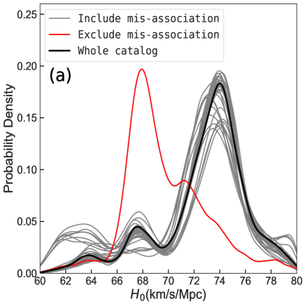
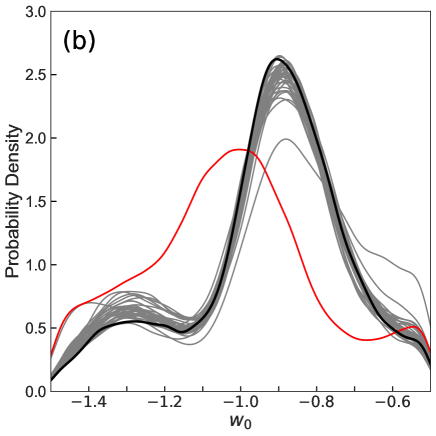
Figure 15: A consistency check on an example catalog, showing marginalized posterior distributions of $H_{0}$ [panel (a)] and $w_{0}$ [panel (b)]. In each panel, the black line represents the result for the whole catalog, the grey lines represent the results for subsets that include the mis-association, and the red line represents the result for the subset that exclude the mis-association. The obvious deviation of posterior modes between the red line and the grey lines indicates the possible occurrence of a mis-association bias.

VI Conclusions and Outlook

In this paper, we develop a Bayesian analysis framework for constraining the cosmological parameters, using simulated observations of the MBHBs mergers from space-borne GW observatories like TianQin and LISA. We obtain the luminosity distance information directly from the GW observations, while a statistical analysis of simulated galaxy catalogs from EM surveys is used to obtain the corresponding redshift information. With the identification of an explicit EM counterpart, one can indeed perform very precise cosmological measurement. However, we also show that one can still obtain useful cosmological constraints even in the dark standard siren scenario where no EM counterpart exists — provided that Malmquist bias is properly accounted for. Furthermore, if we include the localization and mass information from the GW observation to inform the weighting of candidate host galaxies, making use of the relation between the central MBH mass and the bulge luminosity of the host galaxy, we can significantly improve the cosmological constraints.

For the dark standard siren scenario, we consider two weighting schemes, namely the fiducial method, one with uniform weights for all galaxies within the error box, and the weighted method, the weights related to its location and bulge luminosity. With the weighted method scheme, the precision of cosmological parameter estimates can be greatly improved. In this scheme, TianQin can constrain the Hubble constant $H_{0}$ to a precision of $6.9\%$, $6.5\%$, and $3.3\%$, and the CPL parameter $w_{0}$ to a precision of $36.7\%$, $27.2\%$, and $13.8\%$, for the popIII, Q3d and Q3nod MBHB population models respectively. For TianQin I+II, the $H_{0}$ precision can be improved to $6.0\%$, $6.0\%$, and $2.0\%$, and $w_{0}$ precision can reach $26.6\%$, $29.6\%$, and $8.1\%$ — again for popIII, Q3d, and Q3nod models, respectively. The other parameters like $\Omega_{M}$ and $\Omega_{\Lambda}$ need a larger number of events to be significantly constrained. Under the Q3nod model, using the weighted method, $\Omega_{M}$ and $\Omega_{\Lambda}$ can be constrained to an accuracy of $34.9\%$ and $26.1\%$ for TianQin, and $25.1\%$ and $21.5\%$ for TianQin I+II, respectively. However, $w_{a}$ is always difficult to be constrained in all cases.

LISA can perform similarly to TianQin I+II, but the joint detection of TianQin and LISA can significantly improve the precision of the cosmological parameter estimates relative to the results obtained from an individual detector. Using the weighted method, for TianQin+LISA, the precision of $H_{0}$ improves to $4.7\%$, $5.2\%$, and $1.8\%$, and the precision of $w_{0}$ improves to $19.2\%$, $22.3\%$, and $7.9\%$ for popIII, Q3d, and Q3nod models, respectively; for TianQin I+II+LISA, the precision of $H_{0}$ improves to $3.4\%$, $4.7\%$, and $1.7\%$, and the precision of $w_{0}$ improves to $11.3\%$, $18.9\%$, and $7.5\%$, respectively.

For the EM-bright standard siren scenario, the identification of the EM counterpart can help to pinpoint the redshift, and one can not only gain tighter constraints on $H_{0}$ and $w_{0}$, but also obtain meaningful constraints on the other cosmological parameters, including $\Omega_{M}$, $\Omega_{\Lambda}$, and $w_{a}$.

The constraints on the Hubble constant $H_{0}$ are mainly derived from a few events at low redshift, but high redshift GW events play an important role of smoothing out fluctuations in the $H_{0}$ posterior, as well as helping to constrain the values of $\Omega_{M}$ and $\Omega_{\Lambda}$. The CPL model describes the evolution of the dark energy EoS with redshift, so a combination of the GW events at different redshift is needed to constrain $w_{0}$ and $w_{a}$. We also discuss the application of consistency checks on the estimated cosmological parameters, so that the potential bias caused by a single mis-association of a GW event with its host galaxy could be identified.

There are a number of assumptions, which we adopt that could affect the applicability of our method. For example, we depend strongly on the availability of a relatively complete galaxy catalog, reaching out to a high redshift. While in reality, obtaining a relatively complete galaxy catalog at $z>1.5$ is very challenging, when one considers the small localization area that will be provided by TianQin and/or LISA it seems likely that deep-drilled, a more complete galaxy surveys triggered by GW detections could be carried out in order to alleviate incompleteness issues. We also assume a simple relationship between the MBHs mass and the bulge luminosity. Knowledge of the redshift evolution of this $M_{\rm MBH}-L_{\rm bulge}$ relation could also improve the cosmological constraints by reducing any potential bias arising from adopting this simple relationship. Extra information like stellar velocity dispersion can be used to improve the estimation of MBH mass at the low-mass end through the $M_{\rm MBH}-\sigma$ relation.

In the future there is scope to extend our paper in several ways. For example, a new population model of MBHB mergers can be added for the analysis Barausse:2020mdt . The possible existence of strong gravitational lensing events can also help with pinpointing the redshift of GW events Hannuksela:2020xor ; Yu:2020agu . We also plan to extend the GW cosmology study to more types of GW sources Liu:2020eko ; Fan:2020zhy .

Appendix

Appendix A Decomposition of the multimessenger likelihood function

In this Appendix we provide a detailed derivation of the multimessenger likelihood function, namely Eq. (II.3). We can factorize the left-hand side of Eq. (II.3) as

$$p(D_{i},S,D_{L},z,\alpha,\delta,M_{z},L_{\rm bulge},\vec{\theta}^{\prime},\vec{\phi}^{\prime}|\vec{\Omega},I)$$

$$= p(D_{i},S|D_{L},z,\alpha,\delta,M_{z},L_{\rm bulge},\vec{\theta}^{\prime},\vec{\phi}^{\prime},\vec{\Omega},I)p_{0}(D_{L},z,\alpha,\delta,M_{z},L_{\rm bulge},\vec{\theta}^{\prime},\vec{\phi}^{\prime}|\vec{\Omega},I)$$

$$= p(D_{i}|D_{L},\alpha,\delta,M_{z},\vec{\theta}^{\prime},\vec{\Omega},I)p(S|z,\alpha,\delta,L_{\rm bulge},\vec{\phi}^{\prime},\vec{\Omega},I)p_{0}(D_{L},z,\alpha,\delta,M_{z},L_{\rm bulge},\vec{\theta}^{\prime},\vec{\phi}^{\prime}|\vec{\Omega},I)$$

$$= p(D_{i}|D_{L},\alpha,\delta,M_{z},\vec{\theta}^{\prime},\vec{\Omega},I)p(S|z,\alpha,\delta,L_{\rm bulge},\vec{\phi}^{\prime},\vec{\Omega},I)p_{0}(D_{L}|z,\vec{\Omega},I)p_{0}(M_{z}|z,L_{\rm bulge},\vec{\Omega},I)$$

$$\times p_{0}(z,\alpha,\delta,L_{\rm bulge}|\vec{\Omega},I)p_{0}(\vec{\theta}^{\prime}|\vec{\Omega},I)p_{0}(\vec{\phi}^{\prime}|\vec{\Omega},I)$$

$$= p(D_{i}|D_{L},\alpha,\delta,M_{z},\vec{\theta}^{\prime},I)p(S|z,\alpha,\delta,L_{\rm bulge},\vec{\phi}^{\prime},I)p_{0}(D_{L}|z,\vec{\Omega},I)p_{0}(M_{z}|z,L_{\rm bulge},\vec{\Omega},I)$$

$$\times p_{0}(z,\alpha,\delta,L_{\rm bulge}|\vec{\Omega},I)p_{0}(\vec{\theta}^{\prime}|\vec{\Omega},I)p_{0}(\vec{\phi}^{\prime}|\vec{\Omega},I).$$ (34)

Since the distribution of the GW sources and galaxies reflects the evolution of the Universe, we retain the cosmological parameters in all notation of the prior $p_{0}$.

Appendix B deriving the weights

In this Appendix we provide a detailed expression of weighting coefficients applied to the observed and the supplementary galaxies respectively. For an observed galaxy at sky position and redshift of $(\alpha_{j},\delta_{j},z_{j})$ and with bulge luminosity $L_{\rm bulge}$, the positional weight and the weight of bulge luminosity is given by

$$W_{\textrm{pos}}^{\rm obs}(\alpha_{j},\delta_{j}) \propto\exp\bigg{\{}-\frac{1}{2}\Big{[}\big{(}\alpha_{j}-\bar{\alpha},\delta_{j}-\bar{\delta}\big{)}\Sigma_{\alpha\delta}^{-1}\big{(}\alpha_{j}-\bar{\alpha},\delta_{j}-\bar{\delta}\big{)}^{\rm T}\Big{]}\bigg{\}},$$ (35)

$$W_{\textrm{lum}}^{\textrm{obs}}(L_{{\rm bulge},j},z_{j}) \propto\exp\Bigg{[}-\frac{1}{2}\frac{\left(\log_{10}\big{(}(1+z_{j})\hat{M}(L_{{\rm bulge},j})\big{)}-\log_{10}\bar{M}_{z}\right)^{2}}{\sigma_{\log_{10}M}^{2}}\Bigg{]},$$ (36)

where $\bar{\alpha}$, $\bar{\delta}$ and $\bar{M}_{z}$ are the measurement mean value of the longitude, the latitude and the redshifted total mass of the GW source, respectively, and $\Sigma_{\alpha\delta}=\Gamma_{\alpha\delta}^{-1}$ is the covariance matrix of sky localization of the GW source. For the supplementary galaxy, its sky position and redshift $(\alpha_{j},\delta_{j},z_{j})$ are replaced by the measurement mean $(\bar{\alpha}_{\rm obs},\bar{\delta}_{\rm obs},\bar{z}_{\rm obs})$ of observed galaxies within the divided small region, we defined the weight of bulge luminosity as

$$W_{\textrm{lum}}^{\textrm{sup}}\big{(}\Phi^{\prime}(L_{\rm bulge}),\bar{z}_{\rm obs}\big{)}\equiv\int_{0}^{L_{\rm bulge}^{\rm min}}\Phi^{\prime}(L_{\rm bulge})W_{\textrm{lum}}^{\textrm{obs}}(L_{\rm bulge},\bar{z}_{\rm obs})dL_{\rm bulge},$$ (37)

where $(\bar{\alpha}_{\rm obs},\bar{\delta}_{\rm obs},\bar{z}_{\rm obs})$ and $L_{\rm bulge}^{\rm min}$ have different values for each divided small region.

Appendix C Examples of the cosmological constraints

In this Appendix, we show the typical posterior probability distributions of the cosmological parameters and the parameters of EoS of the dark energy for TianQin under the three population models, i.e., popIII, Q3d, and Q3nod, using the fiducial method and the weighted method, in Figs. C16 and C17, respectively.

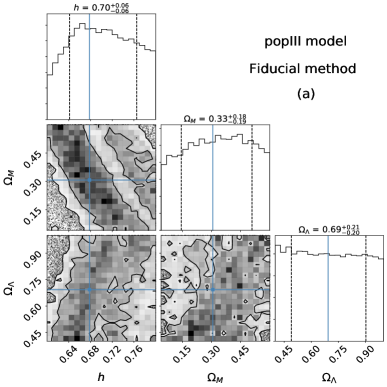
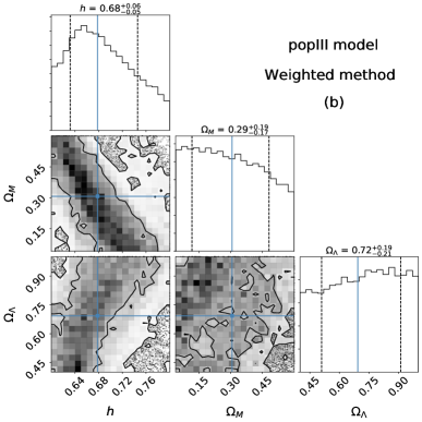
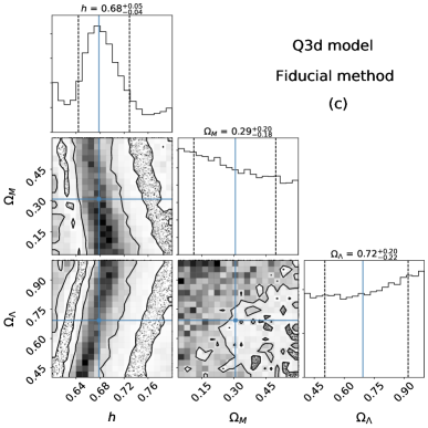
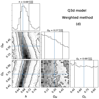
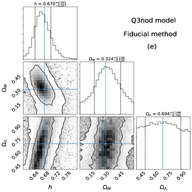
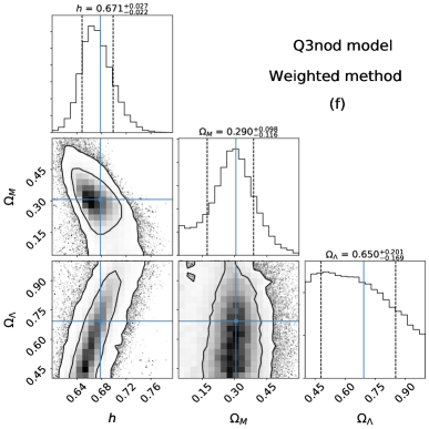
Figure C16: Typical corner plots of the posteriors for the parameters $h$, $\Omega_{M}$, and $\Omega_{\Lambda}$ constrained by the detections of TianQin, comparing the fiducial method (left column) and the weighted method (right column). The top, middle, and bottom rows correspond to adopting popIII, Q3d, and Q3nod respectively as the underlying model for MBHB mergers. In each subplot, the three panels at the lower left show the two-dimensional joint posterior probabilities of $h-\Omega_{M}$, $h-\Omega_{\Lambda}$, and $\Omega_{M}-\Omega_{\Lambda}$, with the contours represent confidence levels of $1\sigma(68.27\%)$ and $2\sigma(95.45\%)$, respectively; the upper, middle and right panels show the one-dimensional posterior probabilities of the corresponding parameters, after marginalization over the other parameters, with the dashed lines indicate $1\sigma$ credible interval. In each panel the solid cyan lines mark the true values of the parameters.

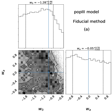
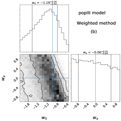
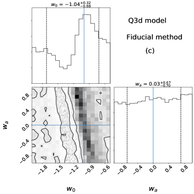
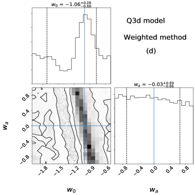
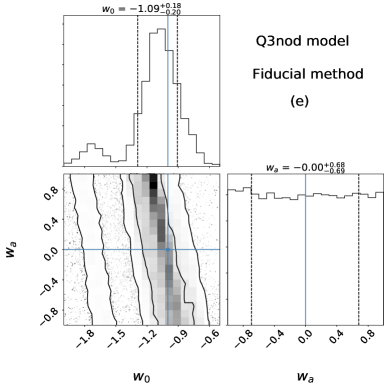
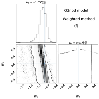
Figure C17: Same as Fig. C16, but for the parameters of EoS of the dark energy $w_{0}$ and $w_{a}$. The other cosmological parameters, $H_{0}$, $\Omega_{M}$, and $\Omega_{\Lambda}$ are fixed.

- [1] B. P. Abbott, R. Abbott, T. D. Abbott, M. R. Abernathy, F. Acernese, K. Ackley, C. Adams, T. Adams, P. Addesso, R. X. Adhikari, and et al. Observation of Gravitational Waves from a Binary Black Hole Merger. Phys. Rev. Lett., 116(6):061102, February 2016.
- [2] B. P. Abbott, R. Abbott, T. D. Abbott, M. R. Abernathy, F. Acernese, K. Ackley, C. Adams, T. Adams, P. Addesso, R. X. Adhikari, and et al. GW151226: Observation of Gravitational Waves from a 22-Solar-Mass Binary Black Hole Coalescence. Phys. Rev. Lett., 116(24):241103, June 2016.
- [3] B. P. Abbott, R. Abbott, T. D. Abbott, F. Acernese, K. Ackley, C. Adams, T. Adams, P. Addesso, R. X. Adhikari, V. B. Adya, and et al. GW170104: Observation of a 50-Solar-Mass Binary Black Hole Coalescence at Redshift 0.2. Phys. Rev. Lett., 118(22):221101, June 2017.
- [4] B. P. Abbott, R. Abbott, T. D. Abbott, F. Acernese, K. Ackley, C. Adams, T. Adams, P. Addesso, R. X. Adhikari, V. B. Adya, and et al. GW170608: Observation of a 19 Solar-mass Binary Black Hole Coalescence. ApJ, 851(2):L35, December 2017.
- [5] B. P. Abbott, R. Abbott, T. D. Abbott, F. Acernese, K. Ackley, C. Adams, T. Adams, P. Addesso, R. X. Adhikari, V. B. Adya, and et al. GW170814: A Three-Detector Observation of Gravitational Waves from a Binary Black Hole Coalescence. Phys. Rev. Lett., 119(14):141101, October 2017.
- [6] B. P. Abbott, R. Abbott, T. D. Abbott, F. Acernese, K. Ackley, C. Adams, T. Adams, P. Addesso, R. X. Adhikari, V. B. Adya, and et al. GW170817: Observation of Gravitational Waves from a Binary Neutron Star Inspiral. Phys. Rev. Lett., 119(16):161101, October 2017.
- [7] B. P. Abbott, R. Abbott, T. D. Abbott, S. Abraham, F. Acernese, K. Ackley, C. Adams, R. X. Adhikari, V. B. Adya, C. Affeldt, and et al. GWTC-1: A Gravitational-Wave Transient Catalog of Compact Binary Mergers Observed by LIGO and Virgo during the First and Second Observing Runs. Physical Review X, 9(3):031040, July 2019.
- [8] R. Abbott et al. GWTC-2: Compact Binary Coalescences Observed by LIGO and Virgo During the First Half of the Third Observing Run. Phys. Rev. X, 11:021053, 2021.
- [9] B. P. Abbott et al. Binary Black Hole Population Properties Inferred from the First and Second Observing Runs of Advanced LIGO and Advanced Virgo. Astrophys. J., 882(2):L24, 2019.
- [10] B. P. Abbott, R. Abbott, T. D. Abbott, M. R. Abernathy, F. Acernese, K. Ackley, C. Adams, T. Adams, P. Addesso, R. X. Adhikari, and et al. Astrophysical Implications of the Binary Black-hole Merger GW150914. ApJ, 818(2):L22, February 2016.
- [11] B. P. Abbott, R. Abbott, T. D. Abbott, M. R. Abernathy, F. Acernese, K. Ackley, C. Adams, T. Adams, P. Addesso, R. X. Adhikari, and et al. Tests of General Relativity with GW150914. Phys. Rev. Lett., 116(22):221101, June 2016.
- [12] B. P. Abbott, R. Abbott, T. D. Abbott, F. Acernese, K. Ackley, C. Adams, T. Adams, P. Addesso, R. X. Adhikari, V. B. Adya, and et al. Gravitational Waves and Gamma-Rays from a Binary Neutron Star Merger: GW170817 and GRB 170817A. ApJ, 848(2):L13, October 2017.
- [13] B. P. Abbott, R. Abbott, T. D. Abbott, F. Acernese, K. Ackley, C. Adams, T. Adams, P. Addesso, R. X. Adhikari, V. B. Adya, and et al. Multi-messenger Observations of a Binary Neutron Star Merger. ApJ, 848(2):L12, October 2017.
- [14] B. P. Abbott, R. Abbott, T. D. Abbott, F. Acernese, K. Ackley, C. Adams, T. Adams, P. Addesso, R. X. Adhikari, V. B. Adya, and et al. A gravitational-wave standard siren measurement of the Hubble constant. Nature, 551(7678):85–88, November 2017.
- [15] Kenta Hotokezaka, Ehud Nakar, Ore Gottlieb, Samaya Nissanke, Kento Masuda, Gregg Hallinan, Kunal P. Mooley, and Adam.T. Deller. A Hubble constant measurement from superluminal motion of the jet in GW170817. Nature Astron., 3(10):940–944, 2019.
- [16] M. Fishbach et al. A Standard Siren Measurement of the Hubble Constant from GW170817 without the Electromagnetic Counterpart. Astrophys. J. Lett., 871(1):L13, 2019.
- [17] M. Soares-Santos et al. First Measurement of the Hubble Constant from a Dark Standard Siren using the Dark Energy Survey Galaxies and the LIGO/Virgo Binary–Black-hole Merger GW170814. ApJ, 876(1):L7, May 2019.
- [18] B. P. Abbott et al. A Gravitational-wave Measurement of the Hubble Constant Following the Second Observing Run of Advanced LIGO and Virgo. Astrophys. J., 909(2):218, 2021.
- [19] A. Palmese et al. A statistical standard siren measurement of the Hubble constant from the LIGO/Virgo gravitational wave compact object merger GW190814 and Dark Energy Survey galaxies. Astrophys. J. Lett., 900(2):L33, 2020.
- [20] B. F. Schutz. Determining the Hubble constant from gravitational wave observations. Nature, 323(6086):310–311, September 1986.
- [21] Adam G. Riess, Lucas M. Macri, Samantha L. Hoffmann, Dan Scolnic, Stefano Casertano, Alexei V. Filippenko, Brad E. Tucker, Mark J. Reid, David O. Jones, Jeffrey M. Silverman, Ryan Chornock, Peter Challis, Wenlong Yuan, Peter J. Brown, and Ryan J. Foley. A 2.4% Determination of the Local Value of the Hubble Constant. ApJ, 826(1):56, July 2016.
- [22] Adam G. Riess, Stefano Casertano, Wenlong Yuan, Lucas M. Macri, and Dan Scolnic. Large Magellanic Cloud Cepheid Standards Provide a 1% Foundation for the Determination of the Hubble Constant and Stronger Evidence for Physics beyond CDM. Astrophys. J., 876(1):85, 2019.
- [23] Wendy L. Freedman, Barry F. Madore, Dylan Hatt, Taylor J. Hoyt, In Sung Jang, Rachael L. Beaton, Christopher R. Burns, Myung Gyoon Lee, Andrew J. Monson, Jillian R. Neeley, M. M. Phillips, Jeffrey A. Rich, and Mark Seibert. The Carnegie-Chicago Hubble Program. VIII. An Independent Determination of the Hubble Constant Based on the Tip of the Red Giant Branch. The Astrophysical Journal, 882(1):34, 2019.
- [24] N. Aghanim et al. Planck 2018 results. VI. Cosmological parameters. Astron. Astrophys., 641:A6, 2020.
- [25] Wendy L. Freedman. Cosmology at a Crossroads. Nat. Astron., 1:0121, 2017.
- [26] L. Verde, T. Treu, and A. G. Riess. Tensions between the Early and the Late Universe. Nature Astron., 3:891, 7 2019.
- [27] Adam G. Riess. The Expansion of the Universe is Faster than Expected. Nature Rev. Phys., 2(1):10–12, 2019.
- [28] Adam G. Riess, Stefano Casertano, Wenlong Yuan, J. Bradley Bowers, Lucas Macri, Joel C. Zinn, and Dan Scolnic. Cosmic Distances Calibrated to 1% Precision with Gaia EDR3 Parallaxes and Hubble Space Telescope Photometry of 75 Milky Way Cepheids Confirm Tension with CDM. Astrophys. J. Lett., 908(1):L6, 2021.
- [29] Stephen M. Feeney, Hiranya V. Peiris, Andrew R. Williamson, Samaya M. Nissanke, Daniel J. Mortlock, Justin Alsing, and Dan Scolnic. Prospects for resolving the Hubble constant tension with standard sirens. Phys. Rev. Lett., 122(6):061105, 2019.
- [30] Wen Zhao. Gravitational-wave standard siren and cosmology (in Chinese). SCIENTIA SINICA Physica, Mechanica & Astronomica, 48(7):079805, July 2018.
- [31] M. Sereno, A. Sesana, A. Bleuler, Ph. Jetzer, M. Volonteri, and M.C. Begelman. Strong lensing of gravitational waves as seen by LISA. Phys. Rev. Lett., 105:251101, 2010.
- [32] M. Sereno, Ph. Jetzer, A. Sesana, and M. Volonteri. Cosmography with strong lensing of LISA gravitational wave sources. Mon. Not. Roy. Astron. Soc., 415:2773, 2011.
- [33] Kai Liao, Xi-Long Fan, Xu-Heng Ding, Marek Biesiada, and Zong-Hong Zhu. Precision cosmology from future lensed gravitational wave and electromagnetic signals. Nature Commun., 8(1):1148, 2017. [Erratum: Nature Commun. 8, 2136 (2017)].
- [34] Stephen R. Taylor, Jonathan R. Gair, and Ilya Mandel. Hubble without the Hubble: Cosmology using advanced gravitational-wave detectors alone. Phys. Rev. D, 85:023535, 2012.
- [35] Stephen R. Taylor and Jonathan R. Gair. Cosmology with the lights off: standard sirens in the Einstein Telescope era. Phys. Rev. D, 86:023502, 2012.
- [36] Will M. Farr, Maya Fishbach, Jiani Ye, and Daniel Holz. A Future Percent-Level Measurement of the Hubble Expansion at Redshift 0.8 With Advanced LIGO. Astrophys. J. Lett., 883(2):L42, 2019.
- [37] Zhi-Qiang You, Xing-Jiang Zhu, Gregory Ashton, Eric Thrane, and Zong-Hong Zhu. Standard-siren cosmology using gravitational waves from binary black holes. Astrophys. J., 908(2):215, 2021.
- [38] Xuheng Ding, Marek Biesiada, Xiaogang Zheng, Kai Liao, Zhengxiang Li, and Zong-Hong Zhu. Cosmological inference from standard sirens without redshift measurements. JCAP, 04:033, 2019.
- [39] Walter Del Pozzo, Tjonnie G. F. Li, and Chris Messenger. Cosmological inference using only gravitational wave observations of binary neutron stars. Phys. Rev. D, 95(4):043502, 2017.
- [40] C. Messenger and J. Read. Measuring a cosmological distance-redshift relationship using only gravitational wave observations of binary neutron star coalescences. Phys. Rev. Lett., 108:091101, 2012.
- [41] C. Messenger, Kentaro Takami, Sarah Gossan, Luciano Rezzolla, and B. S. Sathyaprakash. Source Redshifts from Gravitational-Wave Observations of Binary Neutron Star Mergers. Phys. Rev. X, 4(4):041004, 2014.
- [42] Naoki Seto, Seiji Kawamura, and Takashi Nakamura. Possibility of direct measurement of the acceleration of the universe using 0.1-Hz band laser interferometer gravitational wave antenna in space. Phys. Rev. Lett., 87:221103, 2001.
- [43] Atsushi Nishizawa, Atsushi Taruya, and Shun Saito. Tracing the redshift evolution of Hubble parameter with gravitational-wave standard sirens. Phys. Rev. D, 83:084045, 2011.
- [44] Atsushi Nishizawa, Kent Yagi, Atsushi Taruya, and Takahiro Tanaka. Cosmology with space-based gravitational-wave detectors: Dark energy and primordial gravitational waves. Phys. Rev. D, 85:044047, 2012.
- [45] T. Akutsu et al. KAGRA: 2.5 Generation Interferometric Gravitational Wave Detector. Nature Astron., 3(1):35–40, 2019.
- [46] C. S. Unnikrishnan. IndIGO and Ligo-India Scope and Plans for Gravitational Wave Research and Precision Metrology in India. International Journal of Modern Physics D, 22(1):1341010, January 2013.
- [47] Samaya Nissanke, Daniel E. Holz, Neal Dalal, Scott A. Hughes, Jonathan L. Sievers, and Christopher M. Hirata. Determining the Hubble constant from gravitational wave observations of merging compact binaries. 7 2013.
- [48] Daniel J. Mortlock, Stephen M. Feeney, Hiranya V. Peiris, Andrew R. Williamson, and Samaya M. Nissanke. Unbiased Hubble constant estimation from binary neutron star mergers. Phys. Rev. D, 100(10):103523, 2019.
- [49] Hsin-Yu Chen, Maya Fishbach, and Daniel E. Holz. A two per cent Hubble constant measurement from standard sirens within five years. Nature, 562(7728):545–547, 2018.
- [50] Salvatore Vitale and Hsin-Yu Chen. Measuring the Hubble constant with neutron star black hole mergers. Phys. Rev. Lett., 121(2):021303, 2018.
- [51] Walter Del Pozzo. Inference of the cosmological parameters from gravitational waves: application to second generation interferometers. Phys. Rev. D, 86:043011, 2012.
- [52] Remya Nair, Sukanta Bose, and Tarun Deep Saini. Measuring the Hubble constant: Gravitational wave observations meet galaxy clustering. Phys. Rev. D, 98(2):023502, 2018.
- [53] Rachel Gray et al. Cosmological Inference using Gravitational Wave Standard Sirens: A Mock Data Challenge. Phys. Rev. D, 101(12):122001, 2020.
- [54] M. Punturo et al. The Einstein Telescope: A third-generation gravitational wave observatory. Class. Quant. Grav., 27:194002, 2010.
- [55] Benjamin P Abbott et al. Exploring the Sensitivity of Next Generation Gravitational Wave Detectors. Class. Quant. Grav., 34(4):044001, 2017.
- [56] B.S. Sathyaprakash, B.F. Schutz, and C. Van Den Broeck. Cosmography with the Einstein Telescope. Class. Quant. Grav., 27:215006, 2010.
- [57] Josiel Mendonça Soares de Souza and Riccardo Sturani. Cosmological model selection from standard siren detections by third-generation gravitational wave observatories. Physics of the Dark Universe, 32:100830, 2021.
- [58] W. Zhao, C. Van Den Broeck, D. Baskaran, and T.G.F. Li. Determination of Dark Energy by the Einstein Telescope: Comparing with CMB, BAO and SNIa Observations. Phys. Rev. D, 83:023005, 2011.
- [59] Rong-Gen Cai and Tao Yang. Estimating cosmological parameters by the simulated data of gravitational waves from the Einstein Telescope. Phys. Rev. D, 95(4):044024, 2017.
- [60] Xuan-Neng Zhang, Ling-Feng Wang, Jing-Fei Zhang, and Xin Zhang. Improving cosmological parameter estimation with the future gravitational-wave standard siren observation from the Einstein Telescope. Phys. Rev. D, 99(6):063510, 2019.
- [61] Minghui Du, Weiqiang Yang, Lixin Xu, Supriya Pan, and David F. Mota. Future constraints on dynamical dark-energy using gravitational-wave standard sirens. Phys. Rev. D, 100(4):043535, 2019.
- [62] Jiming Yu, Yu Wang, Wen Zhao, and Youjun Lu. Hunting for the host galaxy groups of binary black holes and the application in constraining Hubble constant. Mon. Not. Roy. Astron. Soc., 498(2):1786–1800, 2020.
- [63] Marina Seikel, Chris Clarkson, and Mathew Smith. Reconstruction of dark energy and expansion dynamics using Gaussian processes. JCAP, 06:036, 2012.
- [64] Weiqiang Yang, Sunny Vagnozzi, Eleonora Di Valentino, Rafael C. Nunes, Supriya Pan, and David F. Mota. Listening to the sound of dark sector interactions with gravitational wave standard sirens. JCAP, 07:037, 2019.
- [65] Jun Luo et al. TianQin: a space-borne gravitational wave detector. Class. Quant. Grav., 33(3):035010, 2016.
- [66] Jianwei Mei et al. The TianQin project: current progress on science and technology. Prog. Theor. Exp. Phys., page ptaa114, 8 2020.
- [67] Shuai Liu, Yi-Ming Hu, Jian-dong Zhang, and Jianwei Mei. Science with the TianQin observatory: Preliminary results on stellar-mass binary black holes. Phys. Rev. D, 101(10):103027, 2020.
- [68] Hui-Min Fan, Yi-Ming Hu, Enrico Barausse, Alberto Sesana, Jian-dong Zhang, Xuefeng Zhang, Tie-Guang Zi, and Jianwei Mei. Science with the TianQin observatory: Preliminary result on extreme-mass-ratio inspirals. Phys. Rev. D, 102(6):063016, 2020.
- [69] Shun-Jia Huang, Yi-Ming Hu, Valeriya Korol, Peng-Cheng Li, Zheng-Cheng Liang, Yang Lu, Hai-Tian Wang, Shenghua Yu, and Jianwei Mei. Science with the TianQin Observatory: Preliminary results on Galactic double white dwarf binaries. Phys. Rev. D, 102(6):063021, 2020.
- [70] Hai-Tian Wang, Zhen Jiang, Alberto Sesana, Enrico Barausse, Shun-Jia Huang, Yi-Fan Wang, Wen-Fan Feng, Yan Wang, Yi-Ming Hu, Jianwei Mei, and Jun Luo. Science with the TianQin observatory: Preliminary results on massive black hole binaries. Phys. Rev. D, 100(4):043003, August 2019.
- [71] Changfu Shi, Jiahui Bao, Haitian Wang, Jian-dong Zhang, Yiming Hu, Alberto Sesana, Enrico Barausse, Jianwei Mei, and Jun Luo. Science with the TianQin observatory: Preliminary results on testing the no-hair theorem with ringdown signals. Phys. Rev. D, 100(4):044036, 2019.
- [72] Jiahui Bao, Changfu Shi, Haitian Wang, Jian-dong Zhang, Yiming Hu, Jianwei Mei, and Jun Luo. Constraining modified gravity with ringdown signals: an explicit example. Phys. Rev. D, 100(8):084024, 2019.
- [73] Xuefeng Zhang, Chengjian Luo, Lei Jiao, Bobing Ye, Huimin Yuan, Lin Cai, Defeng Gu, Jianwei Mei, and Jun Luo. Effect of Earth-Moon’s gravity on TianQin’s range acceleration noise. Phys. Rev. D, 103(6):062001, 2021.
- [74] Bobing Ye, Xuefeng Zhang, Yanwei Ding, and Yunhe Meng. Eclipse avoidance in TianQin orbit selection. Phys. Rev. D, 103(4):042007, 2021.
- [75] Zhuangbin Tan, Bobing Ye, and Xuefeng Zhang. Impact of orbital orientations and radii on TianQin constellation stability. Int. J. Mod. Phys. D, 29(08):08, 2020.
- [76] Bo-Bing Ye, Xuefeng Zhang, Ming-Yue Zhou, Yan Wang, Hui-Min Yuan, Defeng Gu, Yanwei Ding, Jinxiu Zhang, Jianwei Mei, and Jun Luo. Optimizing orbits for TianQin. Int. J. Mod. Phys. D, 28(09):09, 2019.
- [77] Jun Luo et al. The first round result from the TianQin-1 satellite. Class. Quant. Grav., 37(18):185013, 2020.
- [78] Daniel E. Holz and Scott A. Hughes. Using gravitational-wave standard sirens. Astrophys. J., 629:15–22, 2005.
- [79] Neal Dalal, Daniel E. Holz, Scott A. Hughes, and Bhuvnesh Jain. Short grb and binary black hole standard sirens as a probe of dark energy. Phys. Rev. D, 74:063006, 2006.
- [80] Amaro-Seoane, Pau and Audley, Heather and Babak, Stanislav and Baker, John and Barausse, Enrico and Bender, Peter and Berti, Emanuele and Binetruy, Pierre and Born, Michael and Bortoluzzi, Daniele and Camp, Jordan and Caprini, Chiara and Cardoso, Vitor and Colpi, Monica and Conklin, John and Cornish, Neil and Cutler, Curt and Danzmann, Karsten and Dolesi, Rita and Ferraioli, Luigi and Ferroni, Valerio and Fitzsimons, Ewan and Gair, Jonathan and Gesa Bote, Lluis and Giardini, Domenico and Gibert, Ferran and Grimani, Catia and Halloin, Hubert and Heinzel, Gerhard and Hertog, Thomas and Hewitson, Martin and Holley-Bockelmann, Kelly and Hollington, Daniel and Hueller, Mauro and Inchauspe, Henri and Jetzer, Philippe and Karnesis, Nikos and Killow, Christian and Klein, Antoine and Klipstein, Bill and Korsakova, Natalia and Larson, Shane L and Livas, Jeffrey and Lloro, Ivan and Man, Nary and Mance, Davor and Martino, Joseph and Mateos, Ignacio and McKenzie, Kirk and McWilliams, Sean T and Miller, Cole and Mueller, Guido and Nardini, Germano and Nelemans, Gijs and Nofrarias, Miquel and Petiteau, Antoine and Pivato, Paolo and Plagnol, Eric and Porter, Ed and Reiche, Jens and Robertson, David and Robertson, Norna and Rossi, Elena and Russano, Giuliana and Schutz, Bernard and Sesana, Alberto and Shoemaker, David and Slutsky, Jacob and Sopuerta, Carlos F. and Sumner, Tim and Tamanini, Nicola and Thorpe, Ira and Troebs, Michael and Vallisneri, Michele and Vecchio, Alberto and Vetrugno, Daniele and Vitale, Stefano and Volonteri, Marta and Wanner, Gudrun and Ward, Harry and Wass, Peter and Weber, William and Ziemer, John and Zweifel, Peter. Laser Interferometer Space Antenna. 2017.
- [81] K.G. Arun, Chandrakant Mishra, Chris Van Den Broeck, B.R. Iyer, B.S. Sathyaprakash, and Siddhartha Sinha. LISA as a dark energy probe. Class. Quant. Grav., 26:094021, 2009.
- [82] Stanislav Babak, Jonathan R. Gair, Antoine Petiteau, and Alberto Sesana. Fundamental physics and cosmology with LISA. Class. Quant. Grav., 28:114001, 2011.
- [83] Nicola Tamanini, Chiara Caprini, Enrico Barausse, Alberto Sesana, Antoine Klein, and Antoine Petiteau. Science with the space-based interferometer eLISA. III: probing the expansion of the universe using gravitational wave standard sirens. J. Cosmology Astropart. Phys, 2016(4):002, April 2016.
- [84] Chiara Caprini and Nicola Tamanini. Constraining early and interacting dark energy with gravitational wave standard sirens: the potential of the eLISA mission. JCAP, 10:006, 2016.
- [85] Rong-Gen Cai, Nicola Tamanini, and Tao Yang. Reconstructing the dark sector interaction with LISA. JCAP, 05:031, 2017.
- [86] Renjie Wang, Wen-Hong Ruan, Qing Yang, Zong-Kuan Guo, Rong-Gen Cai, and Bin Hu. Hubble parameter estimation via dark sirens with the LISA-Taiji network. National Science Review, 10 2020.
- [87] Antoine Petiteau, Stanislav Babak, and Alberto Sesana. Constraining the dark energy equation of state using LISA observations of spinning Massive Black Hole binaries. Astrophys. J., 732:82, 2011.
- [88] Koutarou Kyutoku and Naoki Seto. Gravitational-wave cosmography with LISA and the Hubble tension. Phys. Rev., D95(8):083525, 2017.
- [89] Walter Del Pozzo, Alberto Sesana, and Antoine Klein. Stellar binary black holes in the LISA band: a new class of standard sirens. Mon. Not. Roy. Astron. Soc., 475(3):3485–3492, 2018.
- [90] Chelsea L MacLeod and Craig J Hogan. Precision of hubble constant derived using black hole binary absolute distances and statistical redshift information. Physical Review D, 77(4):043512, 2008.
- [91] Danny Laghi, Nicola Tamanini, Walter Del Pozzo, Alberto Sesana, Jonathan Gair, Stanislav Babak, and David Izquierdo-Villalba. Gravitational-wave cosmology with extreme mass-ratio inspirals. Mon. Not. Roy. Astron. Soc., 508(3):4512–4531, 2021.
- [92] S. Kawamura et al. The Japanese space gravitational wave antenna DECIGO. Class. Quant. Grav., 23:S125–S132, 2006.
- [93] Jeff Crowder and Neil J. Cornish. Beyond LISA: Exploring future gravitational wave missions. Phys. Rev. D, 72:083005, 2005.
- [94] Toshiya Namikawa, Atsushi Nishizawa, and Atsushi Taruya. Anisotropies of gravitational-wave standard sirens as a new cosmological probe without redshift information. Phys. Rev. Lett., 116(12):121302, 2016.
- [95] Philip J. Armitage and Priyamvada Natarajan. Accretion during the merger of supermassive black holes. Astrophys. J. Lett., 567:L9–L12, 2002.
- [96] Carlos Palenzuela, Luis Lehner, and Steven L. Liebling. Dual Jets from Binary Black Holes. Science, 329:927, 2010.
- [97] Roman Gold, Vasileios Paschalidis, Milton Ruiz, Stuart L. Shapiro, Zachariah B. Etienne, and Harald P. Pfeiffer. Accretion disks around binary black holes of unequal mass: General relativistic mhd simulations of postdecoupling and merger. Phys. Rev. D, 90:104030, Nov 2014.
- [98] Brian D. Farris, Paul Duffell, Andrew I. MacFadyen, and Zoltn Haiman. Binary black hole accretion during inspiral and merger. Monthly Notices of the Royal Astronomical Society: Letters, 447(1):L80–L84, 12 2014.
- [99] Ling-Feng Wang, Ze-Wei Zhao, Jing-Fei Zhang, and Xin Zhang. A preliminary forecast for cosmological parameter estimation with gravitational-wave standard sirens from TianQin. JCAP, 11:012, 2020.
- [100] Ling-Feng Wang, Shang-Jie Jin, Jing-Fei Zhang, and Xin Zhang. Forecast for cosmological parameter estimation with gravitational-wave standard sirens from the LISA-Taiji network. Sci. China Phys. Mech. Astron., 65(1):210411, 2022.
- [101] Alister W. Graham. The Black Hole Mass - Spheroid Luminosity relation. Mon. Not. Roy. Astron. Soc., 379:711–722, 2007.
- [102] Misty C. Bentz, Bradley M. Peterson, Richard W. Pogge, and Marianne Vestergaard. The Black Hole Mass-Bulge Luminosity Relationship for Active Galactic Nuclei from Reverberation Mapping and Hubble Space Telescope Imaging. Astrophys. J., 694:L166–L170, 2009.
- [103] John Kormendy and Luis C. Ho. Coevolution (Or Not) of Supermassive Black Holes and Host Galaxies. Ann. Rev. Astron. Astrophys., 51:511–653, 2013.
- [104] Yanfei Jiang, Jenny Greene, and Luis Ho. Black Hole Mass and Bulge Luminosity for Low-mass Black Holes. Astrophys. J. Lett., 737:L45, 2011.
- [105] Travis Robson, Neil J. Cornish, and Chang Liu. The construction and use of LISA sensitivity curves. Classical and Quantum Gravity, 36(10):105011, May 2019.
- [106] Michel Chevallier and David Polarski. Accelerating universes with scaling dark matter. Int. J. Mod. Phys. D, 10:213–224, 2001.
- [107] Eric V. Linder. Exploring the expansion history of the universe. Phys. Rev. Lett., 90:091301, 2003.
- [108] Anatoly Klypin, Gustavo Yepes, Stefan Gottlöber, Francisco Prada, and Steffen Heß. MultiDark simulations: the story of dark matter halo concentrations and density profiles. Monthly Notices of the Royal Astronomical Society, 457(4):4340–4359, 02 2016.
- [109] B. S. Sathyaprakash and B. F. Schutz. Physics, Astrophysics and Cosmology with Gravitational Waves. Living Rev. Rel., 12:2, 2009.
- [110] Ilya Mandel, Will M. Farr, and Jonathan R. Gair. Extracting distribution parameters from multiple uncertain observations with selection biases. Mon. Not. Roy. Astron. Soc., 486(1):1086–1093, 2019.
- [111] Lee S. Finn. Detection, measurement, and gravitational radiation. Phys. Rev. D, 46:5236–5249, Dec 1992.
- [112] Judith G. Cohen. Caltech faint galaxy redshift survey xvi: the luminosity function for galaxies in the region of the hdf-north to Z = 1.5. Astrophys. J., 567:672, 2002.
- [113] Danilo Marchesini, Pieter van Dokkum, Ryan Quadri, Gregory Rudnick, Marijn Franx, Paulina Lira, Stijn Wuyts, Eric Gawiser, Daniel Christlein, and Sune Toft. The rest-frame optical luminosity functions of galaxies at 2 z 3.5. Astrophys. J., 656:42–65, 2007.
- [114] R.J. Bouwens et al. UV Luminosity Functions at redshifts 4 to 10: 10000 Galaxies from HST Legacy Fields. Astrophys. J., 803(1):34, 2015.
- [115] K. G. Malmquist. On some relations in stellar statistics. Meddelanden fran Lunds Astronomiska Observatorium Serie I, 100:1–52, March 1922.
- [116] Zheng-Cheng Liang, Yi-Ming Hu, Yun Jiang, Jun Cheng, Jian-dong Zhang, and Jianwei Mei. Science with the TianQin Observatory: Preliminary results on stochastic gravitational-wave background. Phys. Rev. D, 105(2):022001, 2022.
- [117] Wen-Hong Ruan, Chang Liu, Zong-Kuan Guo, Yue-Liang Wu, and Rong-Gen Cai. The LISA-Taiji network. Nature Astron., 4:108–109, 2020.
- [118] Xin-Chun Hu, Xiao-Hong Li, Yan Wang, Wen-Fan Feng, Ming-Yue Zhou, Yi-Ming Hu, Shou-Cun Hu, Jian-Wei Mei, and Cheng-Gang Shao. Fundamentals of the orbit and response for TianQin. Classical and Quantum Gravity, 35(9):095008, May 2018.
- [119] Curt Cutler. Angular resolution of the lisa gravitational wave detector. Phys. Rev. D, 57:7089–7102, Jun 1998.
- [120] Neil J. Cornish and Louis J. Rubbo. LISA response function. Phys. Rev. D, 67(2):022001, January 2003.
- [121] Curt Cutler and Éanna E. Flanagan. Gravitational waves from merging compact binaries: How accurately can one extract the binary’s parameters from the inspiral waveform? Phys. Rev. D, 49:2658–2697, Mar 1994.
- [122] Michele Vallisneri. Use and abuse of the fisher information matrix in the assessment of gravitational-wave parameter-estimation prospects. Physical Review D, 77(4), Feb 2008.
- [123] Christopher M. Hirata, Daniel E. Holz, and Curt Cutler. Reducing the weak lensing noise for the gravitational wave Hubble diagram using the non-Gaussianity of the magnification distribution. Phys. Rev. D, 81:124046, 2010.
- [124] Giulia Cusin and Nicola Tamanini. Characterization of lensing selection effects for LISA massive black hole binary mergers. Mon. Not. Roy. Astron. Soc., 504(3):3610–3618, 2021.
- [125] Bence Kocsis, Zsolt Frei, Zoltan Haiman, and Kristen Menou. Finding the electromagnetic counterparts of cosmological standard sirens. Astrophys. J., 637:27–37, 2006.
- [126] Christopher Gordon, Kate Land, and Anze Slosar. Cosmological Constraints from Type Ia Supernovae Peculiar Velocity Measurements. Phys. Rev. Lett., 99:081301, 2007.
- [127] Jian-hua He. Accurate method to determine the systematics due to the peculiar velocities of galaxies in measuring the Hubble constant from gravitational-wave standard sirens. Phys. Rev. D, 100(2):023527, 2019.
- [128] C. Shapiro, D. J. Bacon, M. Hendry, and B. Hoyle. Delensing gravitational wave standard sirens with shear and flexion maps. Monthly Notices of the Royal Astronomical Society, 404(2):858–866, 05 2010.
- [129] Jakob Jonsson, Ariel Goobar, and Edvard Mortsell. Tuning Gravitationally Lensed Standard Sirens. Astrophys. J., 658:52–59, 2007.
- [130] Stefan Hilbert, Jonathan R. Gair, and Lindsay J. King. Reducing distance errors for standard candles and standard sirens with weak-lensing shear and flexion maps. Mon. Not. Roy. Astron. Soc., 412:1023–1037, 2011.
- [131] Cullan Howlett and Tamara M. Davis. Standard siren speeds: improving velocities in gravitational-wave measurements of . Mon. Not. Roy. Astron. Soc., 492(3):3803–3815, 2020.
- [132] Antoine Klein, Enrico Barausse, Alberto Sesana, Antoine Petiteau, Emanuele Berti, Stanislav Babak, Jonathan Gair, Sofiane Aoudia, Ian Hinder, Frank Ohme, and Barry Wardell. Science with the space-based interferometer elisa: Supermassive black hole binaries. Phys. Rev. D, 93:024003, Jan 2016.
- [133] Enrico Barausse. The evolution of massive black holes and their spins in their galactic hosts. MNRAS, 423(3):2533–2557, July 2012.
- [134] Piero Madau and Martin J. Rees. Massive black holes as Population III remnants. Astrophys. J., 551:L27–L30, 2001.
- [135] Marta Volonteri, Francesco Haardt, and Piero Madau. The Assembly and merging history of supermassive black holes in hierarchical models of galaxy formation. Astrophys. J., 582:559–573, 2003.
- [136] M. Volonteri, G. Lodato, and P. Natarajan. The evolution of massive black hole seeds. Mon. Not. Roy. Astron. Soc., 383:1079, 2008.
- [137] Laura Ferrarese and David Merritt. A Fundamental relation between supermassive black holes and their host galaxies. Astrophys. J. Lett., 539:L9, 2000.
- [138] Theoretical astrophysical observatory. https://tao.asvo.org.au/tao/. A part of the All-Sky Virtual Observatory (ASVO).
- [139] P. A. R. Ade et al. Planck 2015 results. XIII. Cosmological parameters. Astron. Astrophys., 594:A13, 2016.
- [140] Darren J. Croton, Adam R. H. Stevens, Chiara Tonini, Thibault Garel, Maksym Bernyk, Antonio Bibiano, Luke Hodkinson, Simon J. Mutch, Gregory B. Poole, and Genevieve M. Shattow. Semi-Analytic Galaxy Evolution (SAGE): Model Calibration and Basic Results. Astrophys. J. Suppl., 222(2):22, 2016.
- [141] Charlie Conroy, Martin White, and James E. Gunn. The propagation of uncertainties in stellar population synthesis modeling II: The challenge of comparing galaxy evolution models to observations. Astrophys. J., 708:58–70, 2010.
- [142] Mark Hannam, Patricia Schmidt, Alejandro Bohé, Leïla Haegel, Sascha Husa, Frank Ohme, Geraint Pratten, and Michael Pürrer. Simple Model of Complete Precessing Black-Hole-Binary Gravitational Waveforms. Phys. Rev. Lett., 113(15):151101, October 2014.
- [143] Donald G. York et al. The Sloan Digital Sky Survey: Technical Summary. Astron. J., 120:1579–1587, 2000.
- [144] A. Drlica-Wagner et al. Dark Energy Survey Year 1 Results: Photometric Data Set for Cosmology. Astrophys. J. Suppl., 235(2):33, 2018.
- [145] Yan Gong, Xiangkun Liu, Ye Cao, Xuelei Chen, Zuhui Fan, Ran Li, Xiao-Dong Li, Zhigang Li, Xin Zhang, and Hu Zhan. Cosmology from the Chinese Space Station Optical Survey (CSS-OS). Astrophys. J., 883:203, 2019.
- [146] R. Laureijs et al. Euclid Definition Study Report. 10 2011.
- [147] Antonio D. Montero-Dorta and Francisco Prada. The SDSS DR6 Luminosity Functions of Galaxies. Mon. Not. Roy. Astron. Soc., 399:1106–1118, 2009.
- [148] S.M. Faber et al. Galaxy luminosity functions to z~1: DEEP2 vs. COMBO-17 and implications for red galaxy formation. Astrophys. J., 665:265–294, 2007.
- [149] Amir Aghamousa et al. The DESI Experiment Part I: Science,Targeting, and Survey Design. 10 2016.
- [150] O. Ilbert et al. Mass assembly in quiescent and star-forming galaxies since z=4 from UltraVISTA. Astron. Astrophys., 556:A55, 2013.
- [151] Tomas Dahlen et al. A Critical Assessment of Photometric Redshift Methods: A CANDELS Investigation. Astrophys. J., 775:93, 2013.
- [152] Daniel Foreman-Mackey, David W. Hogg, Dustin Lang, and Jonathan Goodman. emcee: The MCMC Hammer. Publ. Astron. Soc. Pac., 125:306–312, 2013.
- [153] Foreman-Mackey et al. emcee v3: A Python ensemble sampling toolkit for affine-invariant MCMC. Journal of Open Source Software, 4:1–2, 2019.
- [154] Wen-Fan Feng, Hai-Tian Wang, Xin-Chun Hu, Yi-Ming Hu, and Yan Wang. Preliminary study on parameter estimation accuracy of supermassive black hole binary inspirals for TianQin. Phys. Rev. D, 99(12):123002, June 2019.
- [155] T.M.C. Abbott et al. Cosmological Constraints from Multiple Probes in the Dark Energy Survey. Phys. Rev. Lett., 122(17):171301, 2019.
- [156] Giampaolo Benevento, Wayne Hu, and Marco Raveri. Can Late Dark Energy Transitions Raise the Hubble constant? Phys. Rev. D, 101(10):103517, 2020.
- [157] G. Alestas, L. Kazantzidis, and L. Perivolaropoulos. tension, phantom dark energy, and cosmological parameter degeneracies. Phys. Rev. D, 101(12):123516, 2020.
- [158] Eleonora Di Valentino, Alessandro Melchiorri, and Olga Mena. Can interacting dark energy solve the tension? Phys. Rev. D, 96(4):043503, 2017.
- [159] Rong-Gen Cai, Zong-Kuan Guo, Li Li, Shao-Jiang Wang, and Wang-Wei Yu. Chameleon dark energy can resolve the Hubble tension. Phys. Rev. D, 103(12):121302, 2021.
- [160] M. Dotti, A. Sesana, and R. Decarli. Massive black hole binaries: dynamical evolution and observational signatures. Adv. Astron., 2012:940568, 2012.
- [161] Bruno Giacomazzo, John G. Baker, M.Coleman Miller, Christopher S. Reynolds, and James R. van Meter. General Relativistic Simulations of Magnetized Plasmas around Merging Supermassive Black Holes. Astrophys. J. Lett., 752:L15, 2012.
- [162] Weimin Yuan et al. Einstein Probe - a small mission to monitor and explore the dynamic X-ray Universe. Proceedings of Science, SWIFT10:006, 2015.
- [163] Mu-Xin Liu, Hui Tong, Yi-Ming Hu, Man Leong Chan, Zhu Liu, Hui Sun, and Martin Hendry. Following up the afterglow: strategy for X-ray observation triggered by gravitational wave events. Res. Astron. Astrophys., 21(12):308, 2022.
- [164] Željko Ivezić et al. LSST: from Science Drivers to Reference Design and Anticipated Data Products. Astrophys. J., 873(2):111, 2019.
- [165] Peng Jiang et al. Commissioning progress of the FAST. Sci. China Phys. Mech. Astron., 62(5):959502, 2019.
- [166] Yi Feng, Di Li, Zheng Zheng, and Chao-Wei Tsai. Supermassive Binary Black Hole Evolution can be traced by a small SKA Pulsar Timing Array. Phys. Rev. D, 102(2):023014, 2020.
- [167] Mohamed H. Abdullah, Anatoly Klypin, and Gillian Wilson. Cosmological Constraints on and from Cluster Abundances Using the GalWCat19 Optical-spectroscopic SDSS Catalog. Astrophys. J., 901(2):90, 2020.
- [168] Shadab Alam et al. The Eleventh and Twelfth Data Releases of the Sloan Digital Sky Survey: Final Data from SDSS-III. Astrophys. J. Suppl., 219(1):12, 2015.
- [169] Bela Abolfathi et al. The Fourteenth Data Release of the Sloan Digital Sky Survey: First Spectroscopic Data from the Extended Baryon Oscillation Spectroscopic Survey and from the Second Phase of the Apache Point Observatory Galactic Evolution Experiment. Astrophys. J. Suppl., 235(2):42, 2018.
- [170] Romina Ahumada et al. The 16th Data Release of the Sloan Digital Sky Surveys: First Release from the APOGEE-2 Southern Survey and Full Release of eBOSS Spectra. Astrophys. J. Suppl., 249(1):3, 2020.
- [171] A. Drlica-Wagner et al. Dark Energy Survey Year 1 Results: Photometric Data Set for Cosmology. Astrophys. J. Suppl., 235(2):33, 2018.
- [172] I. Bartos, A. P. S. Crotts, and S. Márka. Galaxy Survey On the Fly: Prospects of Rapid Galaxy Cataloging to Aid the Electromagnetic Follow-Up of Gravitational Wave Observations. ApJ, 801(1):L1, March 2015.
- [173] Emanuele Sobacchi, Mattia C. Sormani, and Antonio Stamerra. A model for periodic blazars. Mon. Not. Roy. Astron. Soc., 465(1):161–172, 2017.
- [174] Thomas Connor, Eduardo Baados, Daniel Stern, Roberto Decarli, Jan-Torge Schindler, Xiaohui Fan, Emanuele Paolo Farina, Chiara Mazzucchelli, John S. Mulchaey, and Fabian Walter. X-ray Observations of a Quasar/Galaxy Merger. Astrophys. J., 887:171, 2019.
- [175] P. Peñil et al. Systematic Search for -Ray Periodicity in Active Galactic Nuclei Detected by the Fermi Large Area Telescope. Astrophys. J., 896(2):134, 2020.
- [176] Khee-Gan Lee, Alex Krolewski, Martin White, David Schlegel, Peter E. Nugent, Joseph F. Hennawi, Thomas Müller, Richard Pan, J. Xavier Prochaska, Andreu Font-Ribera, Nao Suzuki, Karl Glazebrook, Glenn G. Kacprzak, Jeyhan S. Kartaltepe, Anton M. Koekemoer, Olivier Le Fèvre, Brian C. Lemaux, Christian Maier, Themiya Nanayakkara, R. Michael Rich, D. B. Sanders, Mara Salvato, Lidia Tasca, and Kim-Vy H. Tran. First Data Release of the COSMOS Ly Mapping and Tomography Observations: 3D Ly Forest Tomography at 2.05 z 2.55. Astrophys. J. Suppl., 237(2):31, aug 2018.
- [177] C. Ravoux et al. A tomographic map of the large-scale matter distribution using the eBOSS—Stripe 82 Ly forest. JCAP, 07:010, 2020.
- [178] Yuxiang Qin, Andrei Mesinger, Sarah E. I. Bosman, and Matteo Viel. Reionization and galaxy inference from the high-redshift Ly forest. Mon. Not. Roy. Astron. Soc., 506(2):2390–2407, 2021.
- [179] Natalia Porqueres, Jens Jasche, Guilhem Lavaux, and Torsten Enßlin. Inferring high-redshift large-scale structure dynamics from the Lyman- forest. Astron. Astrophys., 630:A151, 2019.
- [180] Yanfei Jiang, Jenny Greene, Luis Ho, Ting Xiao, and Aaron Barth. The Host galaxies of low-mass black holes. Astrophys. J., 742:68, 2011.
- [181] Ting Xiao, Aaron J. Barth, Jenny E. Greene, Luis C. Ho, Misty C. Bentz, Randi R. Ludwig, and Yanfei Jiang. Exploring the Low-Mass End of The M-Sigma Relation with Active Galaxies. Astrophys. J., 739:28, 2011.
- [182] Xuejian Shen, Philip F. Hopkins, Claude-André Faucher-Giguère, D. M. Alexander, Gordon T. Richards, Nicholas P. Ross, and R. C. Hickox. The bolometric quasar luminosity function at z = 0–7. Mon. Not. Roy. Astron. Soc., 495(3):3252–3275, 2020.
- [183] R.J. McLure et al. A new multi-field determination of the galaxy luminosity function at incorporating the 2012 Hubble Ultra-Deep Field imaging. Mon. Not. Roy. Astron. Soc., 432:2696, 2013.
- [184] T. Boroson. The distribution of luminosity in spiral galaxies. ApJS, 46:177–209, June 1981.
- [185] F. Simien and G. de Vaucouleurs. Systematics of bulge-to-disk ratios. Astrophys. J., 302:564–578, 1986.
- [186] N. Caon, M. Capaccioli, and M. D’Onofrio. On the shape of the light profiles of early type galaxies. Mon. Not. Roy. Astron. Soc., 265:1013, 1993.
- [187] Philip F. Hopkins, Tod R. Lauer, Thomas J. Cox, Lars Hernquist, and John Kormendy. Dissipation and Extra Light in Galactic Nuclei: III. ‘Core’ Ellipticals and ‘Missing’ Light. Astrophys. J. Suppl., 181:486–532, 2009.
- [188] John Kormendy, David B. Fisher, Mark E. Cornell, and Ralf Bender. Structure and Formation of Elliptical and Spheroidal Galaxies. Astrophys. J. Suppl., 182:216–309, 2009.
- [189] Enrico Barausse, Irina Dvorkin, Michael Tremmel, Marta Volonteri, and Matteo Bonetti. Massive Black Hole Merger Rates: The Effect of Kiloparsec Separation Wandering and Supernova Feedback. Astrophys. J., 904(1):16, 2020.
- [190] Otto A. Hannuksela, Thomas E. Collett, Mesut Çalışkan, and Tjonnie G. F. Li. Localizing merging black holes with sub-arcsecond precision using gravitational-wave lensing. Mon. Not. Roy. Astron. Soc., 498(3):3395–3402, 2020.
- [191] Hai Yu, Pengjie Zhang, and Fa-Yin Wang. Strong lensing as a giant telescope to localize the host galaxy of gravitational wave event. Mon. Not. Roy. Astron. Soc., 497(1):204–209, 2020.
- [192] LIGO Scientific Collaboration. LIGO Algorithm Library - LALSuite. free software (GPL), 2018.
- [193] Stéfan van der Walt, S. Chris Colbert, and Gaël Varoquaux. The NumPy Array: A Structure for Efficient Numerical Computation. Comput. Sci. Eng., 13(2):22–30, 2011.
- [194] Pauli Virtanen et al. SciPy 1.0–Fundamental Algorithms for Scientific Computing in Python. Nature Meth., 17:261, 2020.
- [195] John D. Hunter. Matplotlib: A 2D Graphics Environment. Comput. Sci. Eng., 9(3):90–95, 2007.
- [196] Daniel Foreman-Mackey. corner.py: Scatterplot matrices in python. The Journal of Open Source Software, 1(2):24, jun 2016.
- [197] Antony Lewis. GetDist: a Python package for analysing Monte Carlo samples. 10 2019.