Improving the filtering of Branch-And-Bound MDD solver (extended)

Abstract

This paper presents and evaluates two pruning techniques to reinforce the efficiency of constraint optimization solvers based on multi-valued decision-diagrams (MDD). It adopts the branch-and-bound framework proposed by Bergman et al. in 2016 to solve dynamic programs to optimality. In particular, our paper presents and evaluates the effectiveness of the local-bound (LocB) and rough upper-bound pruning (RUB). LocB is a new and effective rule that leverages the approximate MDD structure to avoid the exploration of non-interesting nodes. RUB is a rule to reduce the search space during the development of bounded-width-MDDs. The experimental study we conducted on the Maximum Independent Set Problem (MISP), Maximum Cut Problem (MCP), Maximum 2 Satisfiability (MAX2SAT) and the Traveling Salesman Problem with Time Windows (TSPTW) shows evidence indicating that rough-upper-bound and local-bound pruning have a high impact on optimization solvers based on branch-and-bound with MDDs. In particular, it shows that RUB delivers excellent results but requires some effort when defining the model. Also, it shows that LocB provides a significant improvement automatically; without necessitating any user-supplied information. Finally, it also shows that rough-upper-bound and local-bound pruning are not mutually exclusive, and their combined benefit supersedes the individual benefit of using each technique.

Introduction

Multi-valued Decision Diagrams (MDD) are a generalization of Binary Decision Diagrams (BDD) which have long been used in the verification, e.g., for model checking purposes [10]. Recently, these graphical models have drawn the attention of researchers from the CP and OR communities. The popularity of these decision diagrams (DD) stems from their ability to provide a compact representation of large solution spaces as in the case of the table constraint [29, 34]. One of the research streams which emerged from this increased interest about MDDs is decision-diagram-based optimization (DDO) [5]. Its purpose is to efficiently solve combinatorial optimization problems by exploiting problem structure through DDs. This paper belongs to the DDO sub-field and intends to further improve the efficiency of DDO solvers through the introduction of two bounding techniques: local-bounds pruning (LocB) and rough-upper-bound pruning (RUB).

This paper starts by covering the necessary background on DDO. Then, it presents the local-bound and rough-upper-bound pruning techniques in Sections 2.1 and 2.2. After that, it presents an experimental study which we conducted using ‘ddo’ [17], our open source fast and generic MDD-based optimization library. This experimental study investigates the relevance of RUB and LocB through four disinct NP-hard problems: the Weighted Maximum Independent Set Problem (MISP), Maximum Cut Problem (MCP), Maximum 2 Satisfiability Problem (MAX2SAT) and the Traveling Salesman Problem with Time Windows (TSPTW). Finally, section 4 discusses previous related work before drawing conclusions.

1 Background

The coming paragraphs give an overview of discrete optimization with decision diagrams. Most of the formalism presented here originates from [8]. Still, we reproduce it here for the sake of self-containedness.

Discrete optimization.

A discrete optimization problem is a constraint satisfaction problem with an associated objective function to be maximized. The discrete optimization problem $\mathcal{P}$ is defined as $\max\left\{f(x)\mid x\in D\wedge C(x)\right\}$ where $C$ is a set of constraints, $x=\left\langle x_{0},\dots,x_{n-1}\right\rangle$ is an assignment of values to variables, each of which has an associated finite domain $D_{i}$ s.t. $D=D_{0}\times\dots\times D_{n-1}$ from where the values are drawn. In that setup, the function $f:D\to\mathbb{R}$ is the objective to be maximized.

Among the set of feasible solutions $Sol(\mathcal{P})\subseteq D$ (i.e. satisfying all constraints in $C$), we denote the optimal solution by $x^{*}$. That is, $x^{*}\in Sol(\mathcal{P})$ and $\forall x\in Sol(\mathcal{P}):f(x^{*})\geq f(x)$.

Dynamic programming.

Dynamic programming (DP) was introduced in the mid 50’s by Bellman [3]. This strategy is significantly popular and is at the heart of many classical algorithms (e.g., Dijkstra’s algorithm [12, p.658] or Bellman-Ford’s [12, p.651]).

Even though a dynamic program is often thought of in terms of recursion, it is also natural to consider it as a labeled transition system. In that case, the DP model of a given discrete optimization problem $\mathcal{P}$ consists of:

• a set of state-spaces $S_{0},\dots,S_{n}$ among which one distinguishes the initial state $r$, the terminal state $t$ and the infeasible state $\bot$.

• a set of transition functions $t_{i}:S_{i}\times D_{i}\to S_{i+1}$ for $i=0,\dots,n-1$ taking the system from one state $s^{i}$ to the next state $s^{i+1}$ based on the value $d$ assigned to variable $x_{i}$ (or to $\bot$ if assigning $x_{i}=d$ is infeasible). These functions should never allow one to recover from infeasibility ($t_{i}(\bot,d)=\bot$ for any $d\in D_{i}$).

• a set of transition cost functions $h_{i}:S_{i}\times D_{i}\to\mathbb{R}$ representing the immediate reward of assigning some value $d\in D_{i}$ to the variable $x_{i}$ for $i=0,\dots,n-1$.

• an initial value $v_{r}$.

On that basis, the objective function $f(x)$ of $\mathcal{P}$ can be formulated as follows:

$$\text{maximize~{}}f(x)=v_{r}+\sum_{i=0}^{n-1}h_{i}(s^{i},x_{i})$$

subject to

$$s^{i+1}=t_{i}(s^{i},x_{i})\text{~{}for~{}}i=0,\dots,n-1;x_{i}\in D_{i}\wedge C(x_{i})$$

$$s^{i}\in S_{i}\text{~{}for~{}}i=0,\dots,n$$

where $C(x_{i})$ is a predicate that evaluates to $true$ when the partial assignment $\left\langle x_{0},\dots,x_{i}\right\rangle$ does not violate any constraint in $C$.

The appeal of such a formulation stems from its simplicity and its expressiveness which allows it to effectively capture the problem structure. Moreover, this formulation naturally lends itself to a DD representation; in which case it represents an exact DD encoding the complete set $Sol(\mathcal{P})$.

1.1 Decision diagrams

Because DDO aims at solving constraint optimization problems and not just constraint satisfaction problems, it uses a particular DD flavor known as reduced weighted DD – DD as of now. As initially posed by Hooker[21], DDs can be perceived as a compact representation of the search trees. This is achieved, in this context, by superimposing isomorphic subtrees.

To define our DD more formally, we will slightly adapt the notation from [5]. A DD $\mathcal{B}$ is a layered directed acyclic graph $\mathcal{B}=\left\langle n,U,A,l,d,v,\sigma\right\rangle$ where $n$ is the number of variables from the encoded problem, $U$ is a set of nodes; each of which is associated to some state $\sigma(u)$. The mapping $l:U\to\left\{0\dots n\right\}$ partitions the nodes from $U$ in disjoint layers $L_{0}\dots L_{n}$ s.t. $L_{i}=\left\{u\in U:l(u)=i\right\}$ and the states of all the nodes belonging to the same layer pertain to the same DP-state-space ($\forall u\in L_{i}:\sigma(u)\in S_{i}$ for $i=0,\dots,n$). Also, it should be the case that no two distinct nodes of one same layer have the same state ($\forall u_{1},u_{2}\in L_{i}:u_{1}\neq u_{2}\implies\sigma(u_{1})\neq\sigma(u_{2})$, for $i=0,\dots,n$).

The set $A\subseteq U\times U$ from our formal model is a set of directed arcs connecting the nodes from $U$. Each such arc $a=\left(u_{1},u_{2}\right)$ connects nodes from subsequent layers ($l(u_{1})=l(u_{2})-1$) and should be regarded as the materialization of a branching decision about variable $x_{l(u_{1})}$. This is why all arcs are annotated via the mappings $d:A\to D$ and $v:A\to\mathbb{R}$ which respectively associate a decision and value (weight) with the given arc.

Example 1

An arc $a$ connecting nodes $u_{1}\in L_{3}$ to $u_{2}\in L_{4}$, annotated with $d(a)=6$ and $v(a)=42$ should be understood as the assignment $x_{3}=6$ performed from state $\sigma(u_{1})$. It should also be understood that $t_{3}(\sigma(u_{1}),6)=\sigma(u_{2})$ and the benefit of that assignment is $v(a)=h_{3}(\sigma(u_{1}),6)=42$.

Because each $r$-$t$ path describes an assignment that satisfies $\mathcal{P}$, we will use $Sol(\mathcal{B})$ to denote the set of all the solutions encoded in the r-t paths of DD $\mathcal{B}$. Also, because unsatisfiability is irrecoverable, r-$\bot$ paths are typically omitted from DDs. It follows that a nice property from using a DD representation $\mathcal{B}$ for the DP formulation of a problem $\mathcal{P}$, is that finding $x^{*}$ is as simple as finding the longest r-t path in $\mathcal{B}$ (according to the relation $v$ on arcs).

Exact-MDD.

For a given problem $\mathcal{P}$, an exact MDD $\mathcal{B}$ is an MDD that exactly encodes the solution set $Sol(\mathcal{B})=Sol(\mathcal{P})$ of the problem $\mathcal{P}$. In other words, not only do all r-t paths encode valid solutions of $\mathcal{P}$, but no feasible solution is present in $Sol(\mathcal{P})$ and not in $\mathcal{B}$. An exact MDD for $\mathcal{P}$ can be compiled in a top-down fashion. This naturally follows from the above definition. To that end, one simply proceeds by a repeated unrolling of the transition relations until all variables are assigned.

1.2 Bounded-Size Approximations

In spite of the compactness of their encoding, the construction of DD suffers from a potentially exponential memory requirement in the worst case. Thus, using DDs to exactly encode the solution space of a problem is often intractable. Therefore, one must resort to the use of bounded-size approximation of the exact MDD. These are compiled generically by inserting a call to a width-bounding procedure to ensure that the width (the number $|L_{i}|$ of distinct nodes belonging to the $L_{i}$) of the current layer $L_{i}$ does not exceed a given bound $W$. Depending on the behavior of that procedure, one can either compile a restricted-MDD (= an under-approximation) or a relaxed-MDD (= an over-approximation).

Restricted-MDD: Under-approximation.

A restricted-MDD provides an under-approximation of some exact-MDD. As such, all paths of a restricted-MDD encode valid solutions, but some solutions might be missing from the MDD. This is formally expressed as follows: given the DP formulation of a problem $\mathcal{P}$, $\mathcal{B}$ is a restricted-MDD iff $Sol(\mathcal{B})\subseteq Sol(\mathcal{P})$.

To compile a restricted-MDD, it is sufficient to simply delete certain nodes from the current layer until its width fits within the specified bound $W$. To that end, the width-bounding procedure simply selects a subset of the nodes from $L_{i}$ which are heuristically assumed to have the less impact on the tightness of the bound. Various heuristics have been studied in the literature [7], and minLP was shown to be the heuristic that works best in practice. This heuristic decides to select (hence remove) the nodes having the shortest longest path from the root.

Relaxed-MDD: Over-approximation.

A relaxed-MDD $\mathcal{B}$ provides a bounded-width over-approximation of some exact-MDD. As such, it may hold paths that are no solution to $\mathcal{P}$, the problem being solved. We have thus formally that $Sol(\mathcal{B})\supseteq Sol(\mathcal{P})$.

Compiling a relaxed-MDD requires one to be able to merge several nodes into an inexact one. To that end, we use two operators:

• $\oplus$ which yields a new node combining the states of a selection of nodes so as to over-approximate the states reachable in the selection.

• $\Gamma$ which is used to possibly relax the weight of arcs incident to the selected nodes.

These operators are used as follows. Similar to the restricted-MDDs case, the width-bounding procedure starts by heuristically selecting the least promising nodes and removing them from layer $L_{i}$. Then the states of these selected nodes are combined with one another so as to create a merged node $\mathcal{M}=\oplus(selection)$. After that, the inbound arcs incident to all selected nodes are $\Gamma$-relaxed and redirected towards $\mathcal{M}$. Finally, the result of the merger ($\mathcal{M}$) is added to the layer in place of the initial selection of nodes.

Summary.

Fig. 1 summarizes the information from sections 1.1 and 1.2. It displays the three MDDs corresponding to one same example problem having four variables. The exact MDD (a) encodes the complete solution set and, equivalently, the state space of the underlying DP encoding. One easily notices that the restricted DD (b) is an under approximation of (a) since it achieves its width boundedness by removing nodes d and e and their children (i, j). Among others, it follows that the solution $[x_{0}=0,x_{1}=0,x_{2}=0,x_{3}=0]$ is not represented in (b) even though it exists in (a). Conversely, the relaxed diagram (c) achieves a maximum layer with of 3 by merging nodes d, e and h into a new inexact node $\mathcal{M}$ and by relaxing all arcs entering one of the merged nodes. Because of this, (c) introduces solutions that do not exist in (a) as is for instance the case of the assignment $[x_{0}=0,x_{1}=0,x_{2}=3,x_{3}=1]$. Moreover, because the operators $\oplus$ and $\Gamma$ are correct, the length of the longest path in (c) is an upper bound on the optimal value of the objective function. Indeed, one can see that the length of the longest path in (a) (= the exact optimal solution) has a value of 25 while it amounts to 26 in (c).

Figure 1: The exact (a), restricted (b) and relaxed (c) versions of an MDD with four variables. The width of MDDs (b) and (c) have been bounded to a maximum layer width of three. The decision labels of the arcs are shown above the layers separation lines (dashed). The arc weights are shown below the layer separation lines. The longest path of each MDD is boldfaced. In (c), the node $\mathcal{M}$ is the result of merging nodes d, e and h with the $\oplus$ operator. Arcs that have been relaxed with the $\Gamma$ operator are pictured with a double stroke. Note, because these arcs have been $\Gamma$-relaxed, their value might be greater than that of corresponding arcs in (a), (b). Similarly, all “inexact” nodes feature a double border.

1.3 The Dynamics of Branch-and-Bound with DDs

Being able to derive good lower and upper bounds for some optimization problem $\mathcal{P}$ is useful when the goal is to use these bounds to strengthen algorithms [13, 32, 33]. But it is not the only way these approximations can be used. A complete and efficient branch-and-bound algorithm relying on those approximations was proposed in [8] which we hereby reproduce (Alg. 1).

This algorithm works as follows: at start, the node $r$ is created for the initial state of the problem and placed onto the fringe – a global priority queue that tracks all nodes remaining to explore and orders them from the most to least promising. Then, a loop consumes the nodes from that fringe (line 1), one at a time and explores it until the complete state space has been exhausted. The exploration of a node $u$ inside that loop proceeds as follows: first, one compiles a restricted DD $\underline{\mathcal{B}}$ for the sub-problem rooted in $u$ (line 5). Because all paths in a restricted DD are feasible solutions, when the lower bound $v^{*}(\underline{\mathcal{B}})$ derived from the restricted DD $\underline{\mathcal{B}}$ improves over the current best known solution $\underline{v}$; then the longest path of $\underline{\mathcal{B}}$ (best sol. found in $\underline{\mathcal{B}}$) and its length $v^{*}(\underline{\mathcal{B}})$ are memorized (lines 7-9).

In the event where $\underline{\mathcal{B}}$ is exact (no restriction occurred during the compilation of $\underline{\mathcal{B}}$), it covers the complete state space of the sub-problem rooted in $u$. Which means the processing of $u$ is complete and we may safely move to the next node. When this condition is not met, however, some additional effort is required.In that case, a relaxed DD $\overline{\mathcal{B}}$ is compiled from $u$(line 11). That relaxed DD serves two purposes: first, it is used to derive an upper bound $v^{*}(\overline{\mathcal{B}})$ which is compared to the current best known solution (line 12). This gives us a chance to prune the unexplored state space under $u$ when $v^{*}(\overline{\mathcal{B}})$ guarantees it does not contain any better solution than the current best. The second use of $\overline{\mathcal{B}}$ happens when $v^{*}(\overline{\mathcal{B}})$ cannot provide such a guarantee. In that case, the exact cutset of $\overline{\mathcal{B}}$ is used to enumerate residual sub-problems which are enqueued onto the fringe (lines 13-14).

A cutset for some relaxed DD $\overline{\mathcal{B}}$ is a subset $\mathcal{C}$ of the nodes from $\overline{\mathcal{B}}$ such that any $r-t$ path of $\overline{\mathcal{B}}$ goes through at least one node $\in\mathcal{C}$. Also, a node $u$ is said to be exact iff all its incoming paths lead to the same state $\sigma(u)$. From there, an exact cutset of $\overline{\mathcal{B}}$ is simply a cutset whose nodes are all exact. Based on this definition, it is easy to convince oneself that an exact cutset constitutes a frontier up to which the relaxed DD $\overline{\mathcal{B}}$ and its exact counterpart $\mathcal{B}$ have not diverged. And, because it is a cutset, the nodes composing that frontier cover all paths from both $\mathcal{B}$ and $\overline{\mathcal{B}}$; which guarantees the completeness of Alg. 1 [8].

Any relaxed-MDD admits at least one exact cutset – e.g. the trivial $\left\{r\right\}$ case. Often though, it is not unique and different options exist as to what cutset to use. It was experimentally shown by [8] that most of the time, the Last Exact Layer (LEL) is superior to all other exact cutsets in practice. LEL consists of the deepest layer of the relaxed-MDD having all its nodes exact.

Example 2

In Fig.-1 (c), the first inexact node $\mathcal{M}$ occurs in layer $L_{2}$. Hence, the LEL cutset comprises all nodes (a, b, c) from the layer $L_{1}$. Because $\mathcal{M}$ is inexact, and because it is a parent of nodes i, j and k, these three nodes are considered inexact too.

1:  Create node $r$ and add it to $Fringe$

2:  $\underline{x}\leftarrow\bot$

3:  $\underline{v}\leftarrow-\infty$

4:  while $Fringe$ is not empty do

5:     $u\leftarrow Fringe.pop()$

6:     $\underline{\mathcal{B}}\leftarrow Restricted(u)$

7:     if $v^{*}(\underline{\mathcal{B}})>\underline{v}$ then

8:        $\underline{v}\leftarrow v^{*}(\underline{\mathcal{B}})$

9:        $\underline{x}\leftarrow x^{*}(\underline{\mathcal{B}})$

10:     if $\underline{\mathcal{B}}$ is not exact then

11:        $\overline{\mathcal{B}}\leftarrow Relaxed(u)$

12:        if $v^{*}(\overline{\mathcal{B}})>\underline{v}$ then

13:           for all $u^{\prime}\in\overline{\mathcal{B}}.exact\_cutset()$ do

14:              $Fringe.add(u^{\prime})$

15:  return  $\left(\underline{x},\underline{v}\right)$

Algorithm 1 Branch-And-Bound with DD

1:  Create node $r$ and add it to $Fringe$

2:  $\underline{x}\leftarrow\bot$

3:  $\underline{v}\leftarrow-\infty$

4:  while $Fringe$ is not empty do

5:     $u\leftarrow Fringe.pop()$

6:     if $v|_{u}^{*}\leq\underline{v}$ then

7:        continue

8:     $\underline{\mathcal{B}}\leftarrow Restricted(u)$

9:     if $v^{*}(\underline{\mathcal{B}})>\underline{v}$ then

10:        $\underline{v}\leftarrow v^{*}(\underline{\mathcal{B}})$

11:        $\underline{x}\leftarrow x^{*}(\underline{\mathcal{B}})$

12:     if $\underline{\mathcal{B}}$ is not exact then

13:        $\overline{\mathcal{B}}\leftarrow Relaxed(u)$

14:        if $v^{*}(\overline{\mathcal{B}})>\underline{v}$ then

15:           for all $u^{\prime}\in\overline{\mathcal{B}}.exact\_cutset()$ do

16:              if $v|_{u^{\prime}}^{*}>\underline{v}$ then

17:                 $Fringe.add(u^{\prime})$

18:  return  $\left(\underline{x},\underline{v}\right)$

Algorithm 2 Local bound pruning

2 Improving the filtering of branch-and-bound MDD

In the forthcoming paragraphs, we introduce the local bound and present the rough upper bound: two reasoning techniques to reinforce the pruning strength of Alg. 1.

2.1 Local bounds (LocB)

Conceptually, pruning with local bounds is rather simple: a relaxed MDD $\overline{\mathcal{B}}$ provides us with one upper bound $v^{*}(\overline{\mathcal{B}})$ on the optimal value of the objective function for some given sub-problem. However, in the event where $v^{*}(\overline{\mathcal{B}})$ is greater than the best known lower bound $\underline{v}$ (best current solution) nothing guarantees that all nodes from the exact cutset of $\overline{\mathcal{B}}$ admit a longest path to $t$ with a length of $v^{*}(\overline{\mathcal{B}})$. Actually, this is quite unlikely. This is why we propose to attach a “local” upper bound to each node of the cutset. This local upper bound – denoted $v|_{u}^{*}$ for some cutset node $u$ – simply records the length of the longest r-t path passing through $u$ in the relaxed MDD $\overline{\mathcal{B}}$.

In other words, LocB allows us to refine the information provided by a relaxed DD $\overline{\mathcal{B}}$. On one hand, $\overline{\mathcal{B}}$ provides us with $v^{*}(\overline{\mathcal{B}})$ which is the length of the longest r-t path in $\overline{\mathcal{B}}$. As such, it provides an upper bound on the optimal value that can be reached from the root node of $\overline{\mathcal{B}}$. With the addition of LocB, the relaxed DD provides us with an additional piece of information. For each individual node $u$ in the exact cutset of $\overline{\mathcal{B}}$, it defines the value $v|_{u}^{*}$ which is an upper bound on the value attainable from that node.

As shown in Alg. 2, the value $v|_{u}^{*}$ can prove useful at two different moments. First, in the event where $v|_{u}^{*}\leq\underline{v}$, this value can serve as a justification to not enqueue the subproblem $u$ (line 16) since exhausting this subproblem will yield no better solution than $\underline{v}$. More formally, by definition of a cutset and of LocB, it must be the case that the longest r-t path of $\overline{\mathcal{B}}$ traverses one of the cutset nodes $u$ and thus that $v^{*}(\overline{\mathcal{B}})=v|_{u}^{*}$ (where $v|_{u}^{*}$ is the local bound of $u$). Hence we have: $\exists u\in\text{~{}cutset of~{}}\overline{\mathcal{B}}:v^{*}(\overline{\mathcal{B}})=v|^{*}_{u}$. However, because $v^{*}(\overline{\mathcal{B}})$ is the length of the longest r-t path of $\overline{\mathcal{B}}$, there may exist cutset nodes that only belong to r-t paths shorter than $v^{*}(\overline{\mathcal{B}})$. That is: $\forall u’\in\text{~{}cutset of~{}}\overline{\mathcal{B}}:v^{*}(\overline{\mathcal{B}})\geq v|_{u’}^{*}$. Which is why $v|_{u’}^{*}$ can be stricter than $v^{*}(\overline{\mathcal{B}})$ and hence let LocB be stronger at pruning nodes from the frontier.

The second time when $v|_{u}^{*}$ might come in handy occurs when the node $u$ is popped out of the fringe (line 6). Indeed, because the fringe is a global priority queue, any node that has been pushed on the fringe can remain there for a long period of time. Thus, chances are that the value $\underline{v}$ has increased between the moment when the node was pushed onto the fringe (line 17) and the moment when it is popped out of it. Hence, this gives us an additional chance to completely skip the exploration of the sub-problem rooted in $u$.

Let us illustrate that with the relaxed MDD shown on Fig.3, for which the exact cutset comprises the highlighted nodes $a$ and $b$. Please note that because this scenario may occur at any time during the problem resolution, we will assume that the fringe is not empty when it starts. Assuming that the current best solution $\underline{v}$ is $20$ when one explores the pictured subproblem, we are certain that exploring the subproblem rooted in $a$ is a waste of time, because the local bound $v|_{a}^{*}$ is only $16$. Also, because the fringe was not empty, it might be the case that $b$ was left on the fringe for a long period of time. And because of this, it might be the case that the best known value $\underline{v}$ was improved between the moment when $b$ was pushed on the fringe and the moment when it was popped out of it. Assuming that $\underline{v}$ has improved to $110$ when $b$ is popped out of the fringe, it may safely be skipped because $v|_{b}^{*}$ guarantees that an exploration of $b$ will not yield a better solution than $102$.

Alg. 3 describes the procedure to compute the local bound $v|^{*}_{u}$ of each node $u$ belonging to the exact cutset of a relaxed MDD $\overline{\mathcal{B}}$. Intuitively, this is achieved by doing a bottom-up traversal of $\overline{\mathcal{B}}$, starting at $t$ and stopping when the traversal crosses the last exact layer (line 5). During that bottom-up traversal, the algorithm marks the nodes that are reachable from $t$. This way, it can avoid the traversal of dead-end nodes. Also, Alg. 3 maintains a value $v^{*}_{\uparrow_{t}}(u)$ for each node $u$ it encounters. This value represents the length of the longest u-t path. Afterwards (line 13), it is summed with the length of the longest r-u path $v^{*}_{r-u}$ to derive the exact value of the local bound $v|^{*}_{u}$.

1:  $lel\leftarrow$ Index of the last exact layer

2:  $v^{*}_{\uparrow_{t}}(u)\leftarrow-\infty~{}\text{{for each node}}~{}u\in\overline{\mathcal{B}}$ // init. longest u-t path

3:  $mark(t)\leftarrow$true

4:  $v^{*}_{\uparrow_{t}}(t)\leftarrow 0$ // longest t-t path

5:  for all $i=n$ to $lel$ do

6:     for all node $u\in L_{i}$ do

7:        if $mark(u)$ then

8:           for all arc $a=(u^{\prime},u)$ incident to $u$ do

9:              $mark(u^{\prime})\leftarrow$ true

10:              $v^{*}_{\uparrow_{t}}(u^{\prime})\leftarrow\max(v^{*}_{\uparrow_{t}}(u^{\prime}),v^{*}_{\uparrow_{t}}(u)+v(a))$ // longest u’-t path

11:  for all node $u\in\overline{\mathcal{B}}.exact\_cutset()$ do

12:     if $mark(u)$ then

13:        $v|^{*}_{u}\leftarrow v^{*}_{r-u}+v^{*}_{\uparrow_{t}}(u)$ // longest r-u path + longest u-t path

14:     else

15:        $v|^{*}_{u}\leftarrow-\infty$

Algorithm 3 Computing the local bounds

Caveat for the First Exact Layer Cutset (FEL)

Alg. 3 is sufficient to cope with the cases where $\overline{\mathcal{B}}$ uses either a LEL cutset or an FC cutset. However, in the event where $\overline{\mathcal{B}}$ would implement another strategy – such as ie the First Exact Layer (FEL), then Alg. 3 would need to be adapted and perform a complete backward traversal of $\overline{\mathcal{B}}$. Concretely, this means that line 5 would need to read $\text{for all }i\in n\text{ down to }0$ instead of $\text{down to }lel$. This change is mandatory. Failing to implement it could result in too many nodes being pruned away because of the line 15.

2.1.1 Complexity matters…

As shown in Alg. 3, the computation of the local bound $v|^{*}_{u}$ of some node $u$ from the exact cutset of a relaxed MDD $\overline{\mathcal{B}}$ only requires the ability to remember if $u$ is reachable from $t$ ($mark(u)$) and to sum the lengths of the longest r-u path $v^{*}_{r-u}$ and the longest u-t path $v^{*}_{\uparrow_{t}}(u)$. To that end, it is sufficient to only store one flag and two integers in each node. Thus, the spatial complexity of implementing local bounds is $\Theta(1)$ per node.

Similarly, the backwards traversal of $\overline{\mathcal{B}}$ as performed in Alg. 3 only visits a subset of the nodes and arcs that have been created during the compilation of $\overline{\mathcal{B}}$. The time complexity of Alg. 3 is thus bounded by $O(|U|\times|A|)$. Actually, we even know that this bound is lesser or equal to that of the top-down compilation because the width-bounding procedure reduces the number of nodes in $\overline{\mathcal{B}}$. Hence it reduces the number of nodes potentially visited by Alg. 3. It follows that the use of local bounds has no impact on the time complexity of the derivation of a relaxed MDD.

2.2 Rough upper bound (RUB)

Rough upper bound pruning departs from the following observation: assuming the knowledge of a lower bound $\underline{v}$ on the value of $v^{*}$, and assuming that one is able to swiftly compute a rough upper bound $\overline{v_{s}}$ on the optimal value $v^{*}_{s}$ of the subproblem rooted in state $s$; any node $u$ of a MDD having a rough upper bound $\overline{v_{\sigma(u)}}\leq\underline{v}$ may be discarded as it is guaranteed not to improve the best known solution. This is pretty much the same reasoning that underlies the whole branch-and-bound idea. But here, it is used to prune portions of the search space explored while compiling approximate MDDs.

To implement RUB, it suffices to adapt the MDD compilation procedure (top-down , iterative refinement, …) and introduce a check that avoids creating a node $u^{\prime}$ with state $next$ when $\overline{v_{next}}\leq\underline{v}$.

The key to RUB effectiveness is that RUB is used while compiling the restricted and relaxed DDs. As such, its computation does not directly appear in Alg. 1, but rather is accounted within the compilations of $Restricted(u)$ and $Relaxed(u)$ from Alg. 1. Thus, it really is not used as yet-an-other-bound competing with that of line 12, but instead to speed up the computation of restricted and relaxed DDs. More precisely, this speedup occurs because the compilation of the DDs discards some nodes that would otherwise be added to the next layer of the DD and then further expanded, which are ruled out by RUB. A second benefit of using RUBs is that it helps tightening the bound derived from a relaxed DD (Alg.1 line 12). Because the layers that are generated in a relaxed DD are narrower when applying RUB, there are fewer nodes exceeding the maximum layer width. The operator $\oplus$ hence needs to merge a smaller set of nodes in order to produce the relaxation.

The dynamics of RUB is graphically illustrated by Fig.-3 where the set of highlighted nodes can be safely elided since the (rough) upper bound computed in node $s$ is lesser than the best lower bound.

Figure 2: An example relaxed-MDD having an exact cutset $\left\{a,b\right\}$ with local bounds $v|_{a}^{*}$ and $v|_{b}^{*}$. The nodes with a simple border represent exact nodes and those with a double border represent “inexact” nodes. The edges along the longest path are displayed in bold.

Figure 3: Assuming a lower bound $\underline{v}$ of 100 and a rough upper bound $\overline{v_{s}}$ of 42 for the node $s$, all the highlighted nodes (in red, with a dashed border) may be pruned from the MDD.

2.2.1 Important Note

It is important to understand that because the RUB is computed at each node of each restricted and relaxed MDD compiled during the instance resolution, it must be extremely inexpensive to compute. This is why RUB is best obtained from a fast and simple problem specific procedure.

3 Experimental Study

In order to evaluate the impact of the pruning techniques proposed above, we conducted a series of experiments on four problems. In particular, we conducted experiments on the Maximum Independent Set Problem (MISP), the Maximum Cut Problem (MCP), the Maximum Weighted 2-Satisfiablility Problem (MAX2SAT) and the Traveling Salesman Problem with Time Windows (TSPTW). For the first three problems, we generated sets of random instances which we attempted to solve with different configurations of our own open source solver written in Rust [17]. For TSPTW, we reused openly available sets of benchmarks which are usually used to assess the efficiency of new solvers for TSPTW[27]. Thanks to the generic nature of our framework, the model and all heuristics used to solve the instances were the same for all experiments. This allowed us to isolate the impact of RUB and LocB on the solving performance and neutralize unrelated factors such as variable ordering. Indeed, the only variations between the different solver flavors relate to the presence (or absence) of RUB and LocB. All experiments were run on the same physical machine equipped with an AMD6176 processor and 48GB of RAM. A maximum time limit of 1800 seconds was allotted to each configuration to solve each instance.

The models we used for MISP, MCP and MAX2SAT are direct translations of the ones described in [8]. The details of the RUBs we formulated for these problems are given in the appendixes 0.A, 0.B and 0.C. The DP formulation we used for TSPTW, its relaxation and RUB are detailed in appendix 0.D.

MISP.

To assess the impact of RUB and LocB on MISP, we generated random graphs based on the Erdos-Renyi model G(n, p) [15] with the number of vertices n = 250, 500, 750, 1000, 1250, 1500, 1750 and the probability of having an edge connecting any two vertices p = 0.1, 0.2, … , 0.9. The weight of the edges in the generated graphs were drawn uniformly from the set $\{-5,-4,-3,-2,-1,1,2,3,4,5\}$. We generated 10 instances for each combination of size and density (n, p).

MCP.

In line with the strategy used for MISP, we generated random MCP instances as random graphs based on the Erdos-Renyi model G(n, p). These graphs were generated with the number of vertices n = 30, 40, 50 and the probability p of connecting any two vertices = 0.1, 0.2, 0.3, .., 0.9. The weights of the edges in the generated graphs were drawn uniformly among $\{-1,1\}$. Again, we generated 10 instances per combination n, p.

MAX2SAT.

Similar to the above, we used random graphs based the Erdos-Renyi model G(n, p) to derive MAX2SAT instances. To this end, we produced graphs with n = 60, 80, 100, 200, 400, 1000 (hence instances with 30, 40, 50, 100, 200 and 500 variables) and p = 0.1, 0.2, 0.3, .. , 0.9. For each combination of size (n) and density (p), we generated 10 instances. The weights of the clauses in the generated instances were drawn uniformly from the set $\{1,2,3,5,6,7,8,9,10\}$.

TSPTW.

To evaluate the effectiveness of our rules on TSPTW, we used the 467 instances from the following suites of benchmarks, which are usually used to assess the efficiency of new TSPTW solvers. AFG [2], Dumas [14], Gendreau-Dumas [16], Langevin [26], Ohlmann-Thomas [28], Solomon-Pesant [30] and Solomon-Potvin-Bengio [31].

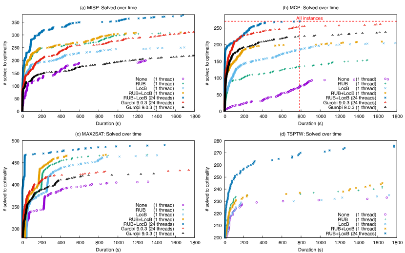
Figure 4: Number of solved instances over time for each considered problem

Figure 4 gives an overview of the results from our experimental study. It respectively depicts the evolution over time of the number of instances solved by each technique for MISP (a), MCP (b) and MAX2SAT (c) and TSPTW (d).

As a first step, our observation of the graphs will focus on the differences that arise between the single threaded configurations of our ddo solvers. Then, in a second phase, we will incorporate an existing state-of-the-art ILP solver (Gurobi 9.0.3) in the comparison. Also, because both Gurobi and our ddo library come with built-in parallel computation capabilities, we will consider both the single threaded and parallel (24 threads) cases. This second phase, however, only bears on MISP, MCP and MAX2SAT by lack of a Gurobi TSPTW model.

DDO configurations

The first observation to be made about the four graphs in Fig.4, is that for all considered problems, both RUB and LocB outperformed the ’do-nothing’ strategy; thereby showing the relevance of the rules we propose. It is not clear however which of the two rules brings the most improvement to the problem resolution. Indeed, RUB seems to be the driving improvement factor for MISP (a) and TSPTW (d) and the impact of LocB appears to be moderate or weak on these problems. However, it has a much higher impact for MCP (b) and MAX2SAT (c). In particular, LocB appears to be the driving improvement factor for MCP (b). This is quite remarkable given that LocB operates in a purely black box fashion, without any problem-specific knowledge. Finally, it should also be noted that the use of RUB and LocB are not mutually exclusive. Moreover, it turns out that for all considered problems, the combination RUB+LocB improved the situation over the use of any single rule.

Furthermore, Fig.5 confirms the benefit of using both RUB and LocB together rather than using any single technique. For each problem, it measures the “performance” of using RUB+LocB vs the best single technique through the end gap. The end gap is defined as $\left(100*\frac{|UB|-|LB|}{|UB|}\right)$. This metric allows us to account for all instances, including the ones that could not be solved to optimality. Basically, a small end gap means that the solver was able to confirm a tight confidence interval of the optimum. Hence, a smaller gap is better. On each subgraphs of Fig.5, the distance along the x-axis represents the end gap for reach instance when using both RUB and LocB whereas the distance along y-axis represents the end gap when using the best single technique for the problem at hand. Any mark above the diagonal shows an instance for which using both RUB and LocB helped reduce the end gap and any mark below that line indicates an instance where it was detrimental.

From graphs 5-a, 5-c and 5-d it appears that the combination RUB+LocB supersedes the use of RUB only. Indeed the vast majority of the marks sit above the diagonal and the rest on it. This indicates a beneficial impact of using both techniques even for the hardest (unsolved) instances. The case of MCP (graph 5-b) is less clear as most of the marks sit on the diagonal. Still, we can only observe three marks below the diagonal and a bit more above it. Which means that even though the use of RUB in addition to LocB is of little help in the case of MCP, its use does not degrade the performance for that considered problem.

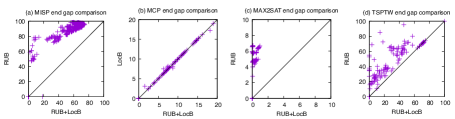
Figure 5: End gap: The benefit of using both techniques vs the best single one

Comparison with Gurobi 9.0.3

The first observation to be made when comparing the performance of Gurobi vs the DDO configurations, is that when running on a single thread, ILP outperforms the basic DDO approach (without RUB and LocB). Furthermore, Gurobi turns out to be the best single threaded solver for MCP by a fair margin. However, in the MISP and MAX2SAT cases, Fig. 4 shows that the DDO solvers benefitting from RUB and LocB were able to solve more instances and to solve them faster than Gurobi. Which underlines the importance of RUB and LocB.

When lifting the one thread limit, one can see that the DD-based approach outperform ILP on each of the considered problems. In particular, in the case of MCP for which Gurobi is the best single threaded option; our DDO solver was able to find and prove the optimality of all tested instances in a little less than 800 seconds. The ILP solver, on the other end, was not able to prove the optimality of the 9 hardest instances within 30 minutes. Additionally, we also observe that in spite of the performance gains of MIP when running in parallel, Gurobi fails to solve as many MISP and MAX2SAT instances and to solve them as fast as the single threaded DDO solvers with RUB and LocB. This emphasizes once more the relevance of our techniques. It also shows that the observation from [9] still hold today: despite the many advances of MIP the DDO approach still scales better than MIP on the considered problems when invoked in parallel.

4 Previous work

DDO emerged in the mid’ 2000’s when [24] proposed to use decision diagrams as a way to solve discrete optimization problems to optimality. More or less concomitantly, [1] devised relaxed-MDD even though the authors envisioned its use as a CP constraint store rather than a means to derive tight upper bounds for optimization problems. Then, the relationship between decision diagrams and dynamic programming was clarified by [21].

Recently, Bergman, Ciré and van Hoeve investigated the various ways to compile decision diagrams for optimization (top-down, construction by separation) [11]. They also investigated the heuristics used to parameterize these DD compilations. In particular, they analyzed the impact of variable ordering in [11, 7] and node selection heuristics (for merge and deletion) in [7]. Doing so, they empirically demonstrated the crucial impact of variable ordering on the tightness of the derived bounds and highlighted the efficiency of minLP as a node selection heuristic. Later on, the same authors proposed a complete branch-and-bound algorithm based on DDs [8]. This is the algorithm which we propose to adapt with extra reasoning mechanisms and for which we provide a generic open-source implementation in Rust [17]. The impressive performance of DDO triggered some theoretical research to analyze the quality of approximate MDDs [5] and the correctness of the relaxation operators [22].

This gave rise to new lines of work. The first one focuses on the resolution of a larger class of optimization problems; chief of which multi-objective problems [4] and problems with a non-linear objective function. These are either solved by decomposition [4] or by using DDO to strengthen other IP techniques [13]. A second trend aims at hybridizing DDO with other IP techniques. For instance, by using Lagrangian relaxation [23] or by solving a MIP [6] to derive with very tight bounds. But the other direction is also under active investigation: for example, [32, 33] use DD to derive tight bounds which are used to replace LP relaxation in a cutting planes solver. Very recently, a third hybridization approach has been proposed by Gonzàlez et al.[18]. It adopts the branch-and-bound MDD perspective, but whenever an upper bound is to be derived, it uses a trained classifier to decide whether the upper bound is to be computed with ILP or by developing a fixed-width relaxed MDD.

The techniques (ILP-cutoff pruning and ILP-cutoff heuristic) proposed by Gonzalez et al.[18] are related to RUB and LocB in the sense that all techniques aim at reducing the search space of the problem. However, they fundamentally differ as ILP-cutoff pruning acts as a replacement for the compilation of a relaxed MDD whereas the goal of RUB is to speed up the development of that relaxed MDD by removing nodes while the MDD is being generated. The difference is even bigger in the case of ILP-cutoff heuristic vs LocB: the former is used as a primal heuristic while LocB is used to filter out sub-problems that can bear no better solution. In that sense, LocB belongs more to the line of work started by [1, 19, 20]: it enforces the constraint $lb\leq f(x)\leq ub$ and therefore provokes the deletion of nodes and arcs that cannot lead to the optimal solution.

More recently, Horn et al explored an idea in [25] which closely relates to RUB. They use “fast-to-compute dual bounds” as an admissible heuristic to guide the compilation of MDDs in an A* fashion for the prize-collecting TSP. It prunes portions of the state space during the MDD construction, similarly to when RUB is applied. Our approach differs from that of [25] in that we attempt to incorporate problem specific knowledge in a framework that is otherwise fully generic. More precisely, it is perceived here as a problem-specific pruning that exploits the combinatorial structure implied by the state variables. It is independent of other MDD compilation techniques, e.g., our techniques are compatible with node merge ($\oplus$) operators and other methodologies defined in the DDO literature. We also emphasize that, as opposed to more complex LP-based heuristics that are now typical in A* search, we investigate quick methodologies that are also easy to incorporate in a MDD branch and bound.

Conclusion and future work

This paper presented and evaluated the impact of the local bound and rough upper bound techniques to strengthen the pruning of the branch-and-bound MDD algorithm. Our experimental study on MISP, MCP, MAX2SAT and TSPTW confirmed the relevance of these techniques. In particular, our experiments have shown that devising a fast and simple rough upper bound is worth the effort as it can significantly boost the efficiency of a solver. Similarly, our experiments showed that the use of local bound can significantly improve the efficiency of DDO solver despite its problem agnosticism. Furthermore, it revealed that a combination of RUB and LocB supersedes the benefit of any single reasoning technique. These results are very promising and we believe that the public availability of an open source DDO framework implementing RUB and LocB might serve as a basis for novel DP formulation for classic problems.

Appendix 0.A MISP

Assuming, the MISP DP formulation from [8], where each state $s$ from the DP model is a bit vector $s_{0}..s_{n}$. And each bit $s_{i}$ from $s$ indicates whether or not the vertex $i$ can possibly be part of the maximum independent set given the decisions labelling the path between the root state $r$ and $s$. The merge operator $\oplus$ simply yields the union of the states that must be combined. The $\Gamma$ operator used to relax edges entering merged node does not alter the weight of these edges.

A RUB for MISP can be computed as

$$\overline{v_{s}}=v^{*}(s)+\sum_{i\in 0..n-1}s_{i}(w_{i})^{+}$$

where $v^{*}(s)$ is the length of the longest $r-s$ path and $w_{i}$ denotes the weight of vertex $i$ and $(w_{i})^{+}=\max(0,w_{i})$. This upper bound is correct because the set of vertices $\left\{i\mid s_{i}=1\right\}$ is a superset of the optimal solution to the subproblem rooted in $s$. (Proof is trivial).

Appendix 0.B MCP

0.B.1 DP model

The DP model we use for the MCP and its relaxation are those from [8]. Their correctness is proved in the same paper. In this model, a state is a tuple of integer values representing the marginal benefit from assigning a vertex to the partition $T$ of the cut.

Formally it is defined as follows:

• State spaces: $S_{k}=\left\{s^{k}\in\mathbb{R}^{n}\mid s^{k}_{j}=0,j=0,\dots,k\right\}$ with root and terminal states equal to $(0,\dots,0)$

• Root value: $v_{r}=\sum_{0\leq i<j<n}(w_{ij})^{-}$

• State transition: $t(s^{k-1},x_{k-1})=(0,\dots,0,s^{k}_{k},\dots,s^{k}_{n-1})$ where

  $$s^{k}_{l}=\left\{\begin{array}[]{ll}s^{k-1}_{l}+w_{kl}&\text{~{}if~{}}x_{k-1}=S\\ s^{k-1}_{l}-w_{kl}&\text{~{}if~{}}x_{k-1}=T\\ \end{array}\right\},l=k,\dots,n-1$$

• Transition cost: $h(s^{0},x_{0})=0$ for $x_{0}\in\left\{S,T\right\}$, and

  $$h(s^{k},x_{k})=\left\{\begin{array}[]{lll}(-s^{k}_{k})^{+}&+\sum_{\begin{subarray}{c}l>k\\ s^{k}_{l}w_{kl}\end{subarray}\leq 0}\min\{|s^{k}_{l}|,|w_{kl}|\},&\text{~{}if~{}}x_{k}=S\\ (s^{k}_{k})^{+}&+\sum_{\begin{subarray}{c}l>k\\ s^{k}_{l}w_{kl}\end{subarray}\leq 0}\min\{|s^{k}_{l}|,|w_{kl}|\},&\text{~{}if~{}}x_{k}=T\\ \end{array}\right\}$$

0.B.2 Relaxation

For the subset $M$ of nodes included in the layer $L_{k}$ of the MDD being compiled, the $\oplus$ and $\Gamma$ operators are defined as follows.

$$\oplus(M)_{l}=\left\{\begin{array}[]{ll}\begin{subarray}{c}\min\left\{u_{l}\right\}\\ u\in M\end{subarray},&\text{~{}if~{}}u_{l}\geq 0\text{~{}for all~{}}u\in M\\ \begin{subarray}{c}-\min\left\{u_{l}\right\}\\ u\in M\end{subarray},&\text{~{}if~{}}u_{l}\leq 0\text{~{}for all~{}}u\in M\\ 0,&\text{otherwise}\end{array}\right\},l=k\dots n-1$$

$$\Gamma_{M}(v,u)=v+\sum_{l\geq k}\left(|u_{l}|-|\oplus(M)_{l}|\right)\text{~{}, for all~{}}u\in M$$

0.B.3 RUB

A RUB for MCP is efficiently computed as follows:

$$\overline{s^{k}}=v^{*}(s^{k})+\sum_{k\leq i<n}|s^{k}_{i}|+\mathcal{V}_{k}+\mathcal{N}_{k}-v_{r}$$

where $s^{k}$ is a state from the $k^{\text{th}}$ layer, $v^{*}(s^{k})$ is the length of the longest $r-s^{k}$ path and $v_{r}$ is the root value of the DP model. $\mathcal{V}_{k}=\sum_{k\leq i<j<n}(w_{ij})^{+}$ is an over estimation of the maximum cut value on the remaining induced graph (sum of the weight of all the positive arcs in the induced graph). $\mathcal{N}_{k}=\sum_{0\leq i<j<k}(w_{ij})^{-}$ is the partial sum of the weights of all negative arcs interconnecting vertices which have already been assigned to a partition.

This upper bound is very fast to compute (amortized $O(n)$) since $v^{*}(s^{k})$ is known when node $s^{k}$ must be expanded and the quantities $v_{r}$, $\mathcal{V}_{k}$ and $\mathcal{N}_{k}$ can be pre-computed once for all (assuming a fixed variable ordering).

Theorem 0.B.1

$$v|^{*}_{s^{k}}\leq\overline{s^{k}}$$

Proof

Because the objective function to maximize is additively separable, we can decompose global problem as a sum of three parts:

1. the longest $r-s^{k}$ path in the subproblem $\mathcal{P}_{0,k}$ bearing only on variables for which a decision has been made $\left[0\dots k-1\right]$. The length of this path is denoted $v^{*}_{\mathcal{P}_{0,k}}(s^{k})$.

2. the value of the best solution to the subproblem $\mathcal{P}_{k,n}$ bearing only on variables for which no decision has been made $\left[k\dots n-1\right]$. We use $v^{*}(\mathcal{P}_{k,n})$ to denote that value.

3. the value $\mathcal{C}_{k}$ of the maximum cut considering only vertices for which a decision has been made $\left[0\dots k-1\right]$ and vertices for which no decision has been made $\left[k\dots n-1\right]$.

Hence, we have $v|^{*}_{s^{k}}=v^{*}_{\mathcal{P}_{0,k}}(s^{k})+v^{*}(\mathcal{P}_{k,n})+\mathcal{C}_{k}$ for any $0\leq k<n$.

According to our decomposition methodology, we would like to start by showing that

$$\begin{array}[]{rl}v^{*}_{\mathcal{P}_{0,k}}(s^{k})&=v^{*}(s^{k})-v_{r}+\mathcal{N}_{k}\\ v_{r}(\mathcal{P}_{0,k})+\sum_{0\leq i<k}h(s^{i},x_{i})&=v^{*}(s^{k})-v_{r}+\mathcal{N}_{k}\\ \sum_{0\leq i<j<k}(w_{ij})^{-}+\sum_{0\leq i<k}h(s^{i},x_{i})&=v^{*}(s^{k})-v_{r}+\mathcal{N}_{k}\\ \mathcal{N}_{k}+\sum_{0\leq i<k}h(s^{i},x_{i})&=v^{*}(s^{k})-v_{r}+\mathcal{N}_{k}\\ \mathcal{N}_{k}+\sum_{0\leq i<k}h(s^{i},x_{i})&=v_{r}+\sum_{0\leq i<k}h(s^{i},x_{i})-v_{r}+\mathcal{N}_{k}\\ \mathcal{N}_{k}+\sum_{0\leq i<k}h(s^{i},x_{i})&=\sum_{0\leq i<k}h(s^{i},x_{i})+\mathcal{N}_{k}\\ \end{array}$$ (1)

Then, we show that

$$v^{*}(\mathcal{P}_{k,n})\leq\mathcal{V}_{k}$$ (2)

By definition of $v^{*}(\mathcal{P}_{k,n})$ as the value of the maximum cut in the residual graph we have: $v^{*}(\mathcal{P}_{k,n})=\max\left\{\sum w_{ij}\mid k\leq i<j<n,x_{i}\neq x_{j}\right\}$. From there, it immediately follows that:

$$\begin{array}[]{rl}v^{*}(\mathcal{P}_{k,n})&\leq\mathcal{V}_{k}\\ \max\left\{\sum w_{ij}\mid k\leq i<j<n,x_{i}\neq x_{j}\right\}&\leq\mathcal{V}_{k}\\ \max\left\{\sum w_{ij}\mid k\leq i<j<n,x_{i}\neq x_{j}\right\}&\leq\sum_{k\leq i<j<n}(w_{ij})^{+}\\ \end{array}$$

Finally, we show that

$$\mathcal{C}_{k}\leq\sum_{k\leq i<n}|s^{k}_{i}|$$ (3)

which is proved by contradiction. Indeed, falsifying that property would require that $\mathcal{C}_{k}>\sum_{k\leq i<n}|s^{k}_{i}|$. That is, it would require that the value of the maximum cut between vertices in $\mathcal{P}_{0,k}$ and those in $\mathcal{P}_{k,n}$ be strictly greater than the sum of the marginal benefit for the ”perfect” assignment of each variable $\geq k$ wrt those $<k$. This either contradicts the definition of a maximum (hence the definition of $\mathcal{C}_{k}$) or that of the state transition function.

Combining (1), (2) and (3); we have

$$\begin{array}[]{c}v^{*}_{\mathcal{P}_{0,k}}(s^{k})=v^{*}(s^{k})-v_{r}+\mathcal{N}_{k}\wedge v^{*}(\mathcal{P}_{k,n})\leq\mathcal{V}_{k}\wedge\mathcal{C}_{k}\leq\sum_{k\leq i<n}|s^{k}_{i}|\\ \implies\\ v^{*}_{\mathcal{P}_{0,k}}(s^{k})+v^{*}(\mathcal{P}_{k,n})+\mathcal{C}_{k}\leq v^{*}(s^{k})+\sum_{k\leq i<n}|s^{k}_{i}|+\mathcal{V}_{k}+\mathcal{N}_{k}-v_{r}\end{array}$$

∎

Appendix 0.C MAX2SAT

The DP model and relaxation we use for MAX2SAT again originates from [8]. Their proof of correctness are to be found in the appendices of the same paper. Because the DP model and relaxation are extremely close for MAX2SAT and MCP, it was decided to omit their detailed formulation from these pages for the sake of conciseness.

0.C.1 RUB

In line with their DP models and relaxations, the RUB definition we used for MAX2SAT is very close to that of MCP. Formally, it is expressed as follows:

$$\overline{s^{k}}=v^{*}(s^{k})+\sum_{k\leq i<n}|s^{k}_{i}|+\mathcal{V}_{k}+\mathcal{N}_{k}-v_{r}$$

where $v_{r}=\sum_{0\leq i<n}w^{i,\neg{i}}$ is the sum of the weights of all tautological clauses in the problem. $\mathcal{N}_{k}$ is used to denote the sum of weights of tautological clauses in the subproblem bearing on assigned literals only. Formally, we have $\mathcal{N}_{k}=\sum_{0\leq i<k}w^{i,\neg{i}}$. Likewise, the definition of $\mathcal{V}_{k}$ is adapted to reflect the MAX2SAT nature of the problem. It is now defined as the sum of the maximal weights for the pairwise assignment of any two undecided variables. This is formally expressed as follows:

$$\begin{array}[]{rcl}\mathcal{V}_{k}&=&\sum_{k\leq i<j<n}\max\left\{w_{ij}^{TT},w_{ij}^{TF},w_{ij}^{FT},w_{ij}^{FF}\right\}\\ &+&\sum_{k\leq i<n}\max\left\{\left(w^{i,\neg i}+w^{i,i}\right),\left(w^{i,\neg i}+w^{\neg i,\neg i}\right)\right\}\\ \end{array}$$

where $w_{ij}^{TT}=w^{i,j}+w^{i,\neg j}+w^{\neg i,j}$ is the total benefit reaped from assigning both variables $i$ and $j$ to true. Likewise, $w_{ij}^{TF},w_{ij}^{FT}$ and $w_{ij}^{FF}$ are defined as follows: $w_{ij}^{TF}=w^{i,j}+w^{i,\neg j}+w^{\neg i,\neg j}$ ; $w_{ij}^{FT}=w^{\neg i,j}+w^{\neg i,\neg j}+w^{i,j}$ ; $w_{ij}^{FF}=w^{\neg i,j}+w^{\neg i,\neg j}+w^{i,\neg j}$.

The proof of correctness for the MAX2SAT RUB is analogous to that of MCP.

Appendix 0.D TSPTW

Important Note

Because TSPTW is a minimization problem, it does not respect the usual DDO maximization assumption. Still, DDO remains perfectly usable provided that relaxed MDD derives a lower bound on the obective value and that RUB (which should rather be called rough lower bound in this case) yields a lower bound on the optimal value rooted in any given node.

0.D.1 DP Model

The DP model we use to solve TSPTW with DDO is a variation of the classical DP formulation that minimizes the makespan. In essence, the model remains exactly the same, only did we adapt the definition of a state to make it more amenable to merging.

Formally, a state $s_{k}$ from the $k$th layer of the MDD is structured as a tuple $\left(position,earliest,latest,must\_visit,may\_visit\right)$ where $position$ is the set of cities where the traveling salesman might possibly be after he visited the $k$ first cities of his tour. As we will show later, this set is – by definition of the transition function – always a singleton except when $s_{k}$ is the state of a merged node. $Earliest$ denotes the earliest time when the salesman could have arrived to some city $\in position$. Conversely, $latest$ denotes the latest moment at which the salesman might have arrived to some city $\in position$. Again, in the absence of relaxed nodes, the time window $\left[earliest,latest\right]$would have a size of $1$ and thus denote an exact duration. Finally, $must\_visit$ is the set of cities that have not been visited on any of the $r-s_{k}$ path, and $may\_visit$ is the set of cities that have been visited along some of the $r-s_{k}$ paths but not all of them.

On that basis, the rest of the DP model is defined as follows:

• Root value: $v_{r}=0$

• Root state: $\left(\{0\},0,0,\left\{1\dots n-1\right\},\emptyset\right)$

• State transition function:

  $$t\left(s_{k},x_{k}\right)=\left(t_{pos}\left(s_{k},x_{k}\right),t_{earliest}\left(s_{k},x_{k}\right),t_{latest}\left(s_{k},x_{k}\right),t_{must}\left(s_{k},x_{k}\right),t_{may}\left(s_{k},x_{k}\right)\right)$$

  where

  $$\begin{array}[]{ll}t_{pos}\left(s_{k},x_{k}\right)&=\left\{x_{k}\right\}\\ t_{must}\left(s_{k},x_{k}\right)&=s_{k}.must\_visit\setminus\left\{x_{k}\right\}\\ t_{may}\left(s_{k},x_{k}\right)&=s_{k}.may\_visit\setminus\left\{x_{k}\right\}\\ t_{earliest}\left(s_{k},x_{k}\right)&=\max\left(earliest(x_{k}),\min\left\{s_{k}.earliest+dist(p,x_{k})\mid p\in s_{k}.position\right\}\right)\\ t_{latest}\left(s_{k},x_{k}\right)&=\min\left(latest(x_{k}),\max\left\{s_{k}.latest+dist(p,x_{k})\mid p\in s_{k}.position\right\}\right)\\ \end{array}$$

• Transition cost function: $h(s_{k},x_{k})=travel(s_{k},x_{k})+wait(s_{k},x_{k})$ where

  $$\begin{array}[]{ll}travel(x_{k},s_{k})&=\min\left\{dist(p,x_{k})\mid p\in s_{k}.position\right\}\\ wait(x_{k},s_{k})&=\left(earliest(x_{k})-s_{k}.earliest+travel(s_{k},x_{k})\right)^{+}\\ \end{array}$$

The state transition and transition cost functions $t(s_{k},x_{k})$ and $h(s_{k},x_{k})$ are only defined when the following three conditions hold:

• $x_{k}\in s_{k}.must\_visit\cup s_{k}.may\_visit$

• $\min\left\{s_{k}.earliest+dist(p,x_{k})\mid p\in s_{k}.position\right\}\leq latest(x_{k})$

• $\max\left\{s_{k}.latest+dist(p,x_{k})\mid p\in s_{k}.position\right\}\geq earliest(x_{k})$

It is obvious that in the absence of relaxation, this model behaves as the classical DP model for TSPTW. Indeed, in that case $position$ is a always a singleton and therefore $earliest$ is always equal to $latest$. Also, one easily sees that $must\_visit$ complements the set of visited cities and $may\_visit$ is always empty.

0.D.2 Relaxation

Our relaxation leverages the structure of the states to perform a merge operation that loses as little information as possible. Our $\Gamma$ operator is defined as the identity function: the cost of edges entering the merged node don’t need to be altered. Our $\oplus$ operator, on the other hand, is slightly more complex. It is defined as follows:

$$\oplus(\mathcal{M})=\left(\oplus_{pos}\left(\mathcal{M}\right),\oplus_{earliest}\left(\mathcal{M}\right),\oplus_{latest}\left(\mathcal{M}\right),\oplus_{must}\left(\mathcal{M}\right),\oplus_{may}\left(\mathcal{M}\right)\right)$$

where

$$\begin{array}[]{ll}\oplus_{pos}\left(\mathcal{M}\right)&=\bigcup_{u\in\mathcal{M}}u.position\\ \oplus_{earliest}\left(\mathcal{M}\right)&=\min\left\{u.earliest\mid u\in\mathcal{M}\right\}\\ \oplus_{latest}\left(\mathcal{M}\right)&=\max\left\{u.latest\mid u\in\mathcal{M}\right\}\\ \oplus_{must}\left(\mathcal{M}\right)&=\bigcap_{u\in\mathcal{M}}u.must\_visit\\ \oplus_{may}\left(\mathcal{M}\right)&=\left(\bigcup_{u\in\mathcal{M}}u.must\_visit\cup u.may\_visit\right)\setminus\left(\bigcap_{u\in\mathcal{M}}u.must\_visit\right)\\ \end{array}$$

0.D.3 RLB (rough lower bound)

First of all, the RLB we compute for TSPTW tries in a quick and inexpensive way to identify infeasible states: those which are guaranteed to enforce a constraint violation sooner or later. In those cases, the RLB returns the $\infty$ value. This approach closely relates to the fail first heuristic implemented in most constraint solvers.

We identified three infeasibility scenarios which can be efficiently checked:

0.D.3.1 Too many unreachable cities

When there are too many cities from the set $may\_visit$ which cannot be reached without violating the time window constraint (it becomes impossible to find a tour visiting $n$ cities without violating the time windows).

$$\begin{array}[]{c}\#\left\{p\mid p\in s^{k}.may\_visit,s^{k}.earliest+shortest\_edge(p)>latest(p)\right\}\\ >\\ n-k-\#s^{k}.must\_visit\\ \end{array}$$

0.D.3.2 One of the mandatory cities cannot be visited

When one of the cities from the $must\_visit$ set cannot be possibly reached without violating its time window constraint.

$$\exists_{p\in s^{k}.must\_visit}s^{k}.earliest+shortest\_edge(p)>latest(p)$$

0.D.3.3 When it is imposible to return to depot in time

This occurs when the elapsed time since the start plus the sum of the shortest edges to each city $p$ makes it impossible to return to depot in due time. Note, $shortest\_edge(p)$ is fixed throughout the whole optimization process as it denotes the shortest path to city $p$ from any other city. The sum $\sum_{p\in s^{k}.must\_visit}shortest\_edge(p)$ is thus an under approximation of the weight of an MST covering the remaining nodes to visit. The tightness loss which occurs vs using the actual weight of an MST is counter balanced by the tiny amount of time required to compute that estimate. This is a worthwhile trade off because of this RUB is computed at least once for every node in the MDD.

$$s^{k}.earliest+\sum_{p\in s^{k}.must\_visit}shortest\_edge(p)>latest(depot)$$

0.D.3.4 Otherwise, when there are still cities to visit

When $s^{k}.must\_visit\neq\emptyset$

$$\begin{array}[]{rl}s^{k}.earliest&+\sum_{p\in s^{k}.must\_visit}shortest\_edge(p)\\ &+min\left\{dist(p,depot)\mid p\in s^{k}.must\_visit\cup s^{k}.may\_visit\right\}\\ >&latest(depot)\\ \end{array}$$

0.D.3.5 Otherwise

When there are no cities left to visit

$$s^{k}.earliest+dist(s^{k}.position,depot)$$

References

- [1] Andersen, H.R., Hadzic, T., Hooker, J.N., Tiedemann, P.: A constraint store based on multivalued decision diagrams. In: Bessière, C. (ed.) Principles and Practice of Constraint Programming. LNCS, vol. 4741, pp. 118–132. Springer (2007)
- [2] Ascheuer, N.: Hamiltonian path problems in the on-line optimization of flexible manufacturing systems (1996)
- [3] Bellman, R.: The theory of dynamic programming. Bulletin of the American Mathematical Society 60(6), 503–515 (11 1954), https://projecteuclid.org:443/euclid.bams/1183519147
- [4] Bergman, D., Cire, A.A.: Multiobjective optimization by decision diagrams. In: Rueher, M. (ed.) Principles and Practice of Constraint Programming. LNCS, vol. 9892, pp. 86–95. Springer (2016)
- [5] Bergman, D., Cire, A.A.: Theoretical insights and algorithmic tools for decision diagram-based optimization. Constraints 21(4), 533–556 (2016). https://doi.org/10.1007/s10601-016-9239-9, https://doi.org/10.1007/s10601-016-9239-9
- [6] Bergman, D., Cire, A.A.: On finding the optimal bdd relaxation. In: Salvagnin, D., Lombardi, M. (eds.) Integration of AI and OR Techniques in Constraint Programming. LNCS, vol. 10335, pp. 41–50. Springer (2017)
- [7] Bergman, D., Cire, A.A., van Hoeve, W.J., Hooker, J.N.: Optimization bounds from binary decision diagrams. INFORMS Journal on Computing 26(2), 253–268 (2014). https://doi.org/10.1287/ijoc.2013.0561, https://doi.org/10.1287/ijoc.2013.0561
- [8] Bergman, D., Cire, A.A., van Hoeve, W.J., Hooker, J.N.: Discrete optimization with decision diagrams. INFORMS Journal on Computing 28(1), 47–66 (2016). https://doi.org/10.1287/ijoc.2015.0648, https://doi.org/10.1287/ijoc.2015.0648
- [9] Bergman, D., Cire, A.A., Sabharwal, A., Samulowitz, H., Saraswat, V., van Hoeve, W.J.: Parallel combinatorial optimization with decision diagrams. International Conference on AI and OR Techniques in Constriant Programming for Combinatorial Optimization Problems pp. 351–367 (2014)
- [10] Burch, J., E.M., C., K.L., M., D.L., D., H.L., H.: Symbolic model checking: states and beyond. Information and Computation 98(2), 142–170 (1992). https://doi.org/10.1016/0890-5401(92)90017-A, https://doi.org/10.1016/0890-5401(92)90017-A
- [11] Cire, A.A.: Decision Diagrams for Optimization. Ph.D. thesis, Carnegie Mellon University Tepper School of Business (2014)
- [12] Cormen, T.H., Leiserson, C.E., Rivest, R.L., Stein, C.: Introduction to algorithms. MIT press (2009)
- [13] Davarnia, D., van Hoeve, W.J.: Outer approximation for integer nonlinear programs via decision diagrams (2018)
- [14] Dumas, Y., Desrosiers, J., Gelinas, E., Solomon, M.M.: An optimal algorithm for the traveling salesman problem with time windows. Operations research 43(2), 367–371 (1995)
- [15] Erdös, P., Rényi, A.: On random graphs i. Publicationes Mathematicae Debrecen 6, 290 (1959)
- [16] Gendreau, M., Hertz, A., Laporte, G., Stan, M.: A generalized insertion heuristic for the traveling salesman problem with time windows. Operations Research 46(3), 330–335 (1998)
- [17] Gillard, X., Schaus, P., Coppé, V.: Ddo, a generic and efficient framework for mdd-based optimization. Accepted at the International Joint Conference on Artificial Intelligence (IJCAI-20); DEMO track (2020)
- [18] Gonzalez, J.E., Cire, A.A., Lodi, A., Rousseau, L.M.: Integrated integer programming and decision diagram search tree with an application to the maximum independent set problem. Constraints pp. 1–24 (2020)
- [19] Hadžić, T., Hooker, J., Tiedemann, P.: Propagating separable equalities in an mdd store. In: CPAIOR. pp. 318–322 (2008)
- [20] Hoda, S., Van Hoeve, W.J., Hooker, J.N.: A systematic approach to mdd-based constraint programming. In: International Conference on Principles and Practice of Constraint Programming. pp. 266–280. Springer (2010)
- [21] Hooker, J.N.: Decision diagrams and dynamic programming. In: Gomes, C., Sellmann, M. (eds.) Integration of AI and OR Techniques in Constraint Programming. LNCS, vol. 7874, pp. 94–110. Springer (2013)
- [22] Hooker, J.N.: Job sequencing bounds from decision diagrams. In: Beck, J.C. (ed.) Principles and Practice of Constraint Programming. LNCS, vol. 10416, pp. 565–578. Springer (2017)
- [23] Hooker, J.N.: Improved job sequencing bounds from decision diagrams. In: Schiex, T., de Givry, S. (eds.) Principles and Practice of Constraint Programming. LNCS, vol. 11802, pp. 268–283. Springer (2019)
- [24] Hooker, J.: Discrete global optimization with binary decision diagrams. GICOLAG 2006 (2006)
- [25] Horn, M., M̃aschler, J., R̃aidl, G.R., R̃önnberg, E.: A*-based construction of decision diagrams for a prize-collecting scheduling problem. Computers & Operations Research 126, 105125 (2021). https://doi.org/https://doi.org/10.1016/j.cor.2020.105125, http://www.sciencedirect.com/science/article/pii/S0305054820302422
- [26] Langevin, A., Desrochers, M., Desrosiers, J., Gélinas, S., Soumis, F.: A two-commodity flow formulation for the traveling salesman and the makespan problems with time windows. Networks 23(7), 631–640 (1993)
- [27] López-Ibáñez, M., Blum, C.: Benchmark instances for the travelling salesman problem with time windows. Online (2020), http://lopez-ibanez.eu/tsptw-instances
- [28] Ohlmann, J.W., Thomas, B.W.: A compressed-annealing heuristic for the traveling salesman problem with time windows. INFORMS Journal on Computing 19(1), 80–90 (2007)
- [29] Perez, G., Régin, J.C.: Efficient operations on mdds for building constraint programming models. In: Proceedings of the Twenty-Fourth International Joint Conference on Artificial Intelligence (IJCAI-15). pp. 374–380 (2015)
- [30] Pesant, G., Gendreau, M., Potvin, J.Y., Rousseau, J.M.: An exact constraint logic programming algorithm for the traveling salesman problem with time windows. Transportation Science 32(1), 12–29 (1998)
- [31] Potvin, J.Y., Bengio, S.: The vehicle routing problem with time windows part ii: genetic search. INFORMS journal on Computing 8(2), 165–172 (1996)
- [32] Tjandraatmadja, C.: Decision Diagram Relaxations for Integer Programming. Ph.D. thesis, Carnegie Mellon University Tepper School of Business (2018)
- [33] Tjandraatmadja, C., van Hoeve, W.J.: Target cuts from relaxed decision diagrams. INFORMS Journal on Computing 31(2), 285–301 (2019). https://doi.org/10.1287/ijoc.2018.0830, https://doi.org/10.1287/ijoc.2018.0830
- [34] Verhaeghe, H., Lecoutre, C., Schaus, P.: Compact-mdd: Efficiently filtering (s) mdd constraints with reversible sparse bit-sets. In: Proceedings of the Twenty-Seventh International Joint Conference on Artificial Intelligence (IJCAI-18). pp. 1383–1389 (2018)