Comment on:“Aharonov-Bohm effect for bound states from the interaction of the magnetic quadrupole moment of a neutral particle with axial fields”. Phys. Rev. A 101, 032102 (2020)

Abstract

We analyze recently published results about the Aharonov-Bohm effect for bound states from the interaction of the magnetic quadrupole moment of a neutral particle with axial fields. We show that the eigenvalues obtained by the authors from an arbitrary truncation of the Frobenius power series correspond to more than one model and, consequently, are unsuitable for drawing any sound physical conclusion. Besides, the prediction of allowed oscillator frequencies is a mere consequence of the truncation condition just mentioned.

In a recent paper Vieira and BakkeVB20 discussed the Aharanov-Bohm effect for the bound states of a neutral particle with a magnetic quadrupole moment that interacts with axial fields. The Schrödinger equation is separable in cylindrical coordinates and the authors applied the Frobenius method to the eigenvalue equation for the radial part. Since the expansion coefficients satisfy a three-term recurrence relation one can, in principle, obtain exact eigenvalues and eigenfunctions from a straightforward truncation condition. They showed that the eigenvalues depend on the geometric quantum phase, which gives rise to an analog of the Ahranov-Bohm effect. In addition, they concluded that each radial mode yields a different set of allowed values of the angular frequency of the harmonic term included in the interaction of one of the models. In this Comment we analyze to which extent the truncation condition affects the physical conclusions drawn in that paper.

The starting point of present discussion is the eigenvalue equation for the radial part of the Schrödinger equation

$$f^{\prime\prime}(y)+\frac{1}{y}f^{\prime}(y)-\frac{\gamma^{2}}{y^{2}}f(y)+\frac{\alpha}{y}f(y)-y^{2}f(y)+Wf(y)=0,$$

$$\gamma^{2}=\left(l+\frac{\phi_{1}}{2\pi}\right)^{2},\;W=\frac{\zeta^{2}}{m\omega},\;\zeta^{2}=2m\mathcal{E}-k^{2},\;\alpha=\frac{MB_{0}}{\sqrt{m\omega}},$$ (1)

where $l=0\pm 1,\pm 2,\ldots$ is the angular momentum quantum number, $m$ the mass of the particle, $\omega$ the oscillator frequency, $\mathcal{E}$ the energy, $\phi_{1}$ the geometric quantum phase, $B_{0}$ a constant in the current density and $M$ the magnitude of the non-null components of the magnetic quadrupole moment. The constant $-\infty<k<\infty$ comes from the fact that the motion is unbounded along the $z$ axis; therefore the spectrum is continuous an bounded from below $\mathcal{E}\geq\frac{\zeta^{2}}{2m}$. The authors simply set $\hbar=1$, $c=1$ though there are well known procedures for obtaining suitable dimensionless equations in a clearer and more rigorous wayF20 . In any case, $y$, $\gamma$, $\alpha$ and $W$ are dimensionless quantities. In what follows we focus on the discrete values of $W$ corresponding to the bound-state solutions of equation (1) that satisfy

$$\int_{0}^{\infty}\left|f(y)\right|^{2}y\,dy<\infty.$$ (2)

Since the behaviour of $f(y)$ at origin is determined by the term $\gamma^{2}/y^{2}$ and its behaviour at infinity by the harmonic term $y^{2}$ we conclude that the eigenvalue equation (1) supports bound states for all $-\infty<\alpha<\infty$. Besides, the eigenvalues $W$ satisfy

$$\frac{\partial W}{\partial\alpha}=-\left\langle\frac{1}{y}\right\rangle<0,$$ (3)

according to the Hellmann-Feynman theoremG32 ; F39 . Since $W(\alpha)$ is a continuous function of $\alpha$ it is clear that the allowed values of the angular frequency $\omega$ were fabricated by Vieira and Bakke by means of the truncation method that we discuss in below.

In order to solve the eigenvalue equation (1) the authors proposed the ansatz

$$f(y)=y^{s}\exp\left(-\frac{y^{2}}{2}\right)H(y),\;H(y)=\sum_{j=0}^{\infty}a_{j}y^{j},\;s=|\gamma|,$$ (4)

and derived the three-term recurrence relation

$$a_{j+2} = -\frac{\alpha}{\left(j+2\right)\left[j+2\left(s+1\right)\right]}a_{j+1}+\frac{\left(2j-\nu\right)}{\left(j+2\right)\left[j+2\left(s+1\right)\right]}a_{j},\;$$

$$\nu = W-2s-2,\;j=-1,0,\ldots,\;a_{-1}=0,\;a_{0}=1.$$ (5)

If the truncation condition $a_{n}\neq 0$, $a_{n+1}=a_{n+2}=0$ has physically acceptable solutions then one obtains some exact eigenvalues and eigenfunctions. The reason is that, under such condition, $a_{j}=0$ for all $j>n$ and the factor $H(y)$ in equation (4) reduces to a polynomial of degree $n$. This truncation condition is equivalent to $\nu=2n$ and $a_{n+1}=0$. The latter equation is a polynomial function of $\alpha$ of degree $n+1$ and it can be proved that all the roots $\alpha_{s}^{(n,i)}$, $i=1,2,\ldots,n+1$, are realCDW00 ; AF20 . For convenience, we order them as $\alpha_{s}^{(n,i)}<\alpha_{s}^{(n,i+1)}$. If $V(\alpha,y)=-\alpha/y+y^{2}$ denotes the parameter-dependent potential for the model discussed here, then it is clear that the truncation condition produces an eigenvalue $W_{s}^{(n)}=2(n+s+1)$ that is common to $n+1$ different potential-energy functions $V_{s}^{(n,i)}(y)=V\left(\alpha_{s}^{(n,i)},y\right)$. Notice that in this analysis we have deliberately omitted part of the interaction that has been absorbed into $\gamma$ (or $s$) because its value is not affected by the truncation approach. Before proceeding with the discussion of this approach we want to point out that the truncation condition only yields some particular eigenvalues and eigenfunctions because not all the solutions $f(y)$ satisfying equation (2) have polynomial factors $H(y)$. This point will be made clearer in the discussion below. From now on, we will refer to them as follows

$$f_{s}^{(n,i)}(y)=y^{s}H_{s}^{(n,i)}(y)\exp\left(-\frac{y^{2}}{2}\right),\;H_{s}^{(n,i)}(y)=\sum_{j=0}^{n}a_{j,s}^{(n,i)}y^{j}.$$ (6)

Present notation takes into account the multiple roots $\alpha_{s}^{(n,i)}$ mentioned above that Vieira and BakkeVB20 appeared to have overlooked.

The authors showed that $H(y)$ is a solution to a biconfluent Heun equation but they did not use its properties to obtain their results and resorted to the Frobenius method and the truncation condition just outlined. For this reason we do not discuss this equation here.

Let us consider the first cases as illustrative examples. When $n=0$ we have $\nu=0$, $\alpha_{s}^{(0)}=0$ and the eigenfunction $f_{s}^{(0)}(y)$ has no nodes. We may consider this case trivial because the problem reduces to the exactly solvable harmonic oscillator. Probably, for this reason it was not explicitly considered by Vieira and BakkeVB20 . However, the results for $\alpha=0$ are also useful for understanding the distribution of the eigenvalues given by the truncation method.

When $n=1$ there are two roots $\alpha_{s}^{(1,1)}=-\sqrt{4s+2}$ and $\alpha_{s}^{(1,2)}=\sqrt{4s+2}$ and the corresponding non-zero coefficients are

$$a_{1,s}^{(1,1)}=\frac{\sqrt{2}}{\sqrt{2s+1}},\;a_{1,s}^{(1,2)}=-\frac{\sqrt{2}}{\sqrt{2s+1}},$$ (7)

respectively. We appreciate that the eigenfunction $f_{s}^{(1,1)}(y)$ is nodeless and $f_{s}^{(1,2)}(y)$ has one node.

When $n=2$ the results are

$$\alpha_{s}^{(2,1)} = -2\sqrt{4s+3},\;a_{1,s}^{(2,1)}=\frac{2\sqrt{4s+3}}{2s+1},\;a_{2,s}^{(2,1)}=\frac{2}{2s+1},$$

$$\alpha_{s}^{(2,2)} = 0,\;a_{1,s}^{(2,2)}=0,\;a_{2,s}^{(2,2)}=-\frac{1}{s+1},$$

$$\alpha_{s}^{(2,3)} = 2\sqrt{4s+3},\;a_{1,s}^{(2,3)}=-\frac{2\sqrt{4s+3}}{2s+1},\;a_{2,s}^{(2,3)}=\frac{2}{2s+1}.$$ (8)

In this case $f_{s}^{(2,1)}(y)$, $f_{s}^{(2,2)}(y)$ and $f_{s}^{(2,3)}(y)$ have zero, one and two nodes, respectively, in the interval $0<y<\infty$. Since Vieira and Bakke overlooked this multiplicity of solutions they missed the actual meaning of the results produced by the truncation approach. For example, one should not forget that these three functions are states of three different quantum mechanical models.

From the results for $n=1$ the authors derived the following equation for the energy

$$\mathcal{E}_{1,l,k} = \omega_{1,l}\left(s+2\right)+\frac{k^{2}}{2m},$$

$$\omega_{1,l} = \frac{M^{2}B_{0}^{2}}{2m(2s+1)},$$ (9)

and stated that “Therefore, not all values of the angular frequency are allowed for a polynomial of first degree”. It is clear that $\mathcal{E}_{1,l,k}$ is an eigenvalue common to the pair of models given by $V_{s}^{(1,i)}(y)$, $i=1,2$, while $\mathcal{E}_{1,l^{\prime},k}$ is an eigenvalue common to a different pair of models given by $V_{s^{\prime}}^{(1,i)}(y)$. Therefore, it is not clear that the results reported by Vieira and Bakke may be useful from a physical point of view. These authors did not appear to understand the actual meaning of the exact solutions to conditionally solvable quantum-mechanical models that one obtains for particular relationships about the model parameters (see, for example, CDW00 ; AF20 ; F20b ; F20c , and in particular the remarkable reviewT16 , and references therein).

As stated above, the eigenvalue equation (1) is not exactly solvable; therefore, in order to obtain its eigenvalues $W_{j,s}$, $j=0,1,\ldots$, $W_{j,s}<W_{j+1,s}$ we should resort to a suitable numerical method. The simplest one appears to be the well known Rayleigh-Ritz variational method that is known to yield increasingly accurate upper bounds to the eigenvalues of a quantum-mechanical modelP68 ; D20 . For present application we choose the non-orthogonal basis set of Gaussian functions $\left\{u_{j,s}(y)=y^{s+j}\exp\left(-\frac{y^{2}}{2}\right),\;j=0,1,\ldots\right\}$.

For simplicity we arbitrarily choose $s=0$ as a first illustrative case. When $\alpha=\alpha_{0}^{(1,1)}=-\sqrt{2}$ the first four eigenvalues are $W_{0,0}=W_{0}^{(1)}=4$, $W_{1,0}=7.693978891$, $W_{2,0}=11.50604238$, $W_{3,0}=15.37592718$; on the other hand, when $\alpha=\alpha_{0}^{(1,2)}=\sqrt{2}$ we have $W_{0,0}=-1.459587134$, $W_{1,0}=W_{0}^{(1)}=4$, $W_{2,0}=8.344349427$, $W_{3,0}=12.53290130$. The rate of convergence of the approach (in terms of the number $N$ of basis functions) is clearly shown in tables 1 and 2. Notice that the truncation condition yields only the ground state for the former model and the first excited state for the latter, missing all the other eigenvalues for each model potential. Compare these numerical results with the discussion about equation (7).

As a second example we choose $s=1$, again to facilitate the calculations. When $\alpha=\alpha_{1}^{(1,1)}=-\sqrt{6}$ the first four eigenvalues are $W_{0,0}=W_{1}^{(1)}=6$, $W_{1,1}=9.805784090$, $W_{2,1}=13.66928892$, $W_{3,1}=17.56601881$; on the other hand, when $\alpha=\alpha_{1}^{(1,2)}=\sqrt{6}$ we have $W_{0,1}=1.600357154$, $W_{1,1}=W_{1}^{(1)}=6$, $W_{2,1}=10.21072810$, $W_{3,1}=14.35078474$. Notice that the truncation condition yields only the lowest state for the former model and the second-lowest one for the latter, missing all the other eigenvalues for each model potential as in the preceding example.

From the analysis above one may draw the wrong conclusion that the truncation condition is utterly useless; however, it has been shown that one can extract valuable information about the spectrum of conditionally solvable models if one arranges and connects the roots $W_{s}^{(n)}$ properlyCDW00 ; AF20 ; F20b ; F20c . From the analysis outlined above we conclude that $\left(\alpha_{s}^{(n,i)},W_{s}^{(n)}\right)$ is a point on the curve $W_{i-1,s}(\alpha)$, $i=1,2,\ldots,n+1$, so that we can easily construct some parts of such spectral curves. For example, Figure 1 shows several eigenvalues $W_{0}^{(n)}$ given by the truncation condition (red circles) and the variational results obtained by means of $N=16$ Gaussian functions (blue lines). We appreciate that the variational results connect the roots of the truncation method. Besides, it is clear that the actual eigenvalues $W_{j,s}(\alpha)$ are continuous functions of $\alpha$ and that the allowed discrete angular frequencies were fabricated by Vieira and Bakke by means of the truncation method that yields some eigenvalues for particular values of $\alpha=\alpha_{s}^{n,i}$ (red circles in Figure 1).

The spectrum of a quantum mechanical problem determined by $V(\alpha,y)$ is given by the intersection of a vertical line through the chosen value of $\alpha$ and the blue lines in Figure 1 (obviously, of the infinite number of the latter lines we only show $7$). Figure 1 shows two such vertical lines (green, dashed). It is worth noticing that any such vertical line will meet only one red point when $\alpha=\alpha_{s}^{(n,i)}$ and none when $\alpha\neq\alpha_{s}^{(n,i)}$ which tells us that the truncation condition gives only one eigenvalue and for a particular model potential. An exception should be made for the trivial case $\alpha=0$ because the truncation condition yields all the eigenvalues of the harmonic oscillator. The reason is that the Frobenius method for the harmonic oscillator leads to a two-term recurrence relation and it can be proved that there are no square-integrable solutions beyond those with polynomial factorsP68 . The origin of the authors’ mistakes appears to be that they think that the approach that gives the whole spectrum of the exactly solvable model ($\alpha=0$) also gives the whole spectrum of the conditionally-solvable one. It is already well known that such an assumption is falseCDW00 ; AF20 ; F20b ; F20c ; T16 .

The Rayleigh-Ritz variational method is extremely reliable and is commonly used for obtaining the most accurate eigenvalues of atomic and molecular systemsP68 ; D20 . However, in order to verify the accuracy of present results we have also applied the powerful Riccati-Padé method (RPM)FMT89a that exhibits exponential convergence. This approach is based on a rational approximation to the power-series expansion of the logarithmic derivative of the wavefunction ($f(y)$ in the present case) and does not exhibit any feature common to the Rayleigh-Ritz variational methodFMT89a . For this reason the RPM is a most reliable and independent test for the results obtained by means of the Rayleigh-Ritz method. A curious feature of the RPM is that, given a value of $\alpha$, it yields the eigenvalues for $\pm\alpha$. Tables 3 and 4 show that the roots of the Hankel determinantsFMT89a converge towards the eigenvalues given by the Rayleigh-Ritz variational method discussed above (tables 1 and 2) as the determinant dimension $D$ increases. Notice that the RPM also yields the exact eigenvalue $W=W_{0}^{(1)}=4$ for $\alpha=\pm\sqrt{2}$.

Finally, we mention that the truncation condition yields only positive eigenvalues $W_{s}^{(n)}$; however, the actual eigenvalues $W_{j,s}(\alpha)$ decrease with $\alpha$ and, eventually, become negative. For example, it is not difficult to show that

$$W_{j,s}(\alpha)\approx-\frac{\alpha^{2}}{\left(2j+2s+1\right)^{2}}+\mathcal{O}\left(\alpha^{-2}\right),\;\alpha\rightarrow\infty.$$ (10)

Notice that the variational results in Figure 1 illustrate this behaviour.

Summarizing: the analytical expression for the energy obtained by the Vieira and Bakke is unsuitable for any physical purpose because any change of the quantum number $l$ transforms the chosen model into another one with a different interaction potential. The dependence of the oscillator frequency on $n$ and $l$ is an artifact of the truncation of the Frobenius series and exhibits no physical meaning whatsoever. Present variational results already show that the eigenvalues are continuous functions of the model parameters and, consequently, the angular frequency can have any positive value. The truncation condition only provides some rare eigenvalues and eigenfunctions with polynomial factors $H_{s}^{(n,i)}(y)$ that by themselves do not represent the spectrum of a single problem but particular solutions of more than one model. Apparently, the authors were unaware of this fact. The origin of the authors’ misunderstanding of the solutions given by the truncation method is the false belief that the eigenfunctions with polynomial factors $H_{s}^{(n,i)}(y)$ are the only possible solutions. Simple inspection of the eigenvalue equation (1), supported by a variational calculation, already shows that most of the eigenfunctions do not exhibit polynomial factors. The truncation condition only yields the whole spectrum for the trivial case $\alpha=0$ and the reason is that in this case the Frobenius method leads to a two-term recurrence relationP68 . In this Comment we have also shown how to extract some useful information from the roots of the truncation condition.

Table 1: Lowest variational eigenvalues $W_{j,0}\left(-\sqrt{2}\right)$

$N$	$W_{0,0}$	$W_{1,0}$	$W_{2,0}$	$W_{3,0}$
$2$	$4.000000000$	$10.49997602$
$3$	$4.000000000$	$7.751061995$	$19.88102859$
$4$	$4.000000000$	$7.694010921$	$11.97562584$	$33.92039998$
$5$	$4.000000000$	$7.693979367$	$11.51212379$	$17.05520450$
$6$	$4.000000000$	$7.693978905$	$11.50604696$	$15.46896992$
$7$	$4.000000000$	$7.693978892$	$11.50604243$	$15.37652840$
$8$	$4.000000000$	$7.693978891$	$11.50604238$	$15.37592761$
$9$	$4.000000000$	$7.693978891$	$11.50604238$	$15.37592718$
$10$	$4.000000000$	$7.693978891$	$11.50604238$	$15.37592718$

Table 2: Lowest variational eigenvalues $W_{j,0}\left(\sqrt{2}\right)$

$N$	$W_{0,0}$	$W_{1,0}$	$W_{2,0}$	$W_{3,0}$
$2$	$-1.180391283$	$4.000000000$
$3$	$-1.401182256$	$4.000000000$	$9.284143096$
$4$	$-1.449885589$	$4.000000000$	$8.345259771$	$17.66452696$
$5$	$-1.458156835$	$4.000000000$	$8.344361267$	$12.69095166$
$6$	$-1.459389344$	$4.000000000$	$8.344349784$	$12.53313315$
$7$	$-1.459560848$	$4.000000000$	$8.344349442$	$12.53290257$
$8$	$-1.459583736$	$4.000000000$	$8.344349427$	$12.53290132$
$9$	$-1.459586704$	$4.000000000$	$8.344349427$	$12.53290130$
$10$	$-1.459587081$	$4.000000000$	$8.344349427$	$12.53290130$
$11$	$-1.459587128$	$4.000000000$	$8.344349427$	$12.53290130$
$12$	$-1.459587134$	$4.000000000$	$8.344349427$	$12.53290130$
$13$	$-1.459587134$	$4.000000000$	$8.344349427$	$12.53290130$

Table 3: Lowest RPM eigenvalues $W_{j,0}\left(-\sqrt{2}\right)$

$D$	$W_{0,0}$	$W_{1,0}$	$W_{2,0}$	$W_{3,0}$
$8$	$4.000000000$	$7.693449704$	$11.16567414$
$9$	$4.000000000$	$7.693990279$	$11.54430665$	$15.16153572$
$10$	$4.000000000$	$7.693978617$	$11.50547430$	$15.12357546$
$11$	$4.000000000$	$7.693978898$	$11.50605268$	$15.41617482$
$12$	$4.000000000$	$7.693978891$	$11.50604217$	$15.37544063$
$13$	$4.000000000$	$7.693978891$	$11.50604238$	$15.37593481$
$14$	$4.000000000$	$7.693978891$	$11.50604238$	$15.37592704$
$15$	$4.000000000$	$7.693978891$	$11.50604238$	$15.37592718$

Table 4: Lowest RPM eigenvalues $W_{j,0}\left(\sqrt{2}\right)$

$D$	$W_{0,0}$	$W_{1,0}$	$W_{2,0}$	$W_{3,0}$
$8$	$-1.459586733$	$4.000000000$	$8.413675510$	$12.38593112$
$9$	$-1.459587149$	$4.000000000$	$8.343322691$	$12.35721732$
$10$	$-1.459587134$	$4.000000000$	$8.344372803$	$12.62125942$
$11$	$-1.459587135$	$4.000000000$	$8.344348852$	$12.53183748$
$12$	$-1.459587134$	$4.000000000$	$8.344349441$	$12.53292129$
$13$	$-1.459587134$	$4.000000000$	$8.344349426$	$12.53290088$
$14$	$-1.459587134$	$4.000000000$	$8.344349427$	$12.53290131$
$15$	$-1.459587134$	$4.000000000$	$8.344349427$	$12.53290130$

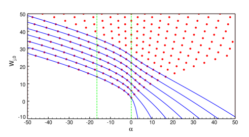
Figure 1: Eigenvalues $W_{j,0}$ obtained from the truncation condition (red circles) and from the variational method (blue lines)

References

- (1) S. L. R. Vieira and K. Bakke, Phys. Rev. A 101, 032102 (2020).
- (2) F. M. Fernández, Dimensionless equations in non-relativistic quantum mechanics, arXiv:2005.05377 [quant-ph].
- (3) P. Güttinger, Z. Phys. 73, 169 (1932).
- (4) R. P. Feynman, Phys. Rev. 56, 340 (1939).
- (5) M. S. Child, S-H. Dong, and X-G. Wang, J. Phys. A 33, 5653 (2000).
- (6) P. Amore and F. M. Fernández, On some conditionally solvable quantum-mechanical problems,arXiv:2007.03448 [quant-ph].
- (7) F. M. Fernández, The rotating harmonic oscillator revisited, arXiv:2007.11695 [quant-ph].
- (8) F. M. Fernández, The truncated Coulomb potential revisited, .arXiv:2008.01773 [quant-ph].
- (9) A. V. Turbiner, Phys. Rep. 642, 1 (2016). arXiv:1603.02992v2
- (10) F. L. Pilar, Elementary Quantum Chemistry (McGraw-Hill, New York, 1968).
- (11) G. W. F. Drake, J. Phys. B 53, 223001 (2020).
- (12) F. M. Fernández, Q. Ma, and R. H. Tipping, Phys. Rev. A 39, 1605 (1989).