Optimization of Controlled-$Z$ Gate with Data-Driven Gradient Ascent Pulse Engineering in a Superconducting Qubit System

Abstract

The experimental optimization of a two-qubit controlled-$Z$ (CZ) gate is realized following two different data-driven gradient ascent pulse engineering (GRAPE) protocols in the aim of optimizing the gate operator and the output quantum state, respectively. For both GRAPE protocols, the key computation of gradients utilizes mixed information of the input $Z$-control pulse and the experimental measurement. With an imperfect initial pulse in a flattop waveform, our experimental implementation shows that the CZ gate is quickly improved and the gate fidelities subject to the two optimized pulses are around 99%. Our experimental study confirms the applicability of the data-driven GRAPE protocols in the problem of the gate optimization.

I Introduction

The realization of high-fidelity quantum gates is essential in quantum computation and quantum simulation [1]. As an important one in the group of fundamental quantum gates, the two-qubit controlled-NOT (CNOT) gate can be experimentally created by the combination of a two-qubit controlled-$Z$ (CZ) gate and two single-qubit gates [2, 3, 4, 5, 6]. The recent advancements in technology have allowed precise control and measurement of quantum devices. The superconducting qubit system has reached $<\!1\%$ errors below the fault-tolerant threshold of surface code quantum computing [7, 2, 8]. In our previous study of the CZ gate, the gate fidelity is $\sim 94\%$ for a shortcut-to-adiabaticity (STA) pulse [9]. Although such an external pulse with an analytic form is experimentally available [10, 11], the state-of-the-art high-fidelity gate still needs optimization algorithms due to unavoidable control distortion. In a previous work by Martinis and his coworkers, the fidelity of the CZ gate reaches $>99\%$ under an optimal fast adiabatic pulse [8]. This optimization is realized by a randomized benchmarking (RB) based Nelder-Mead learning algorithm [8, 12]. In a RB experiment, the statistical average of the ground-state population over sequences of random Clifford gates is utilized to identify the fidelity of a specific quantum gate [13, 14, 15]. Following a test-and-trial strategy, the Nelder-Mead algorithm searches the parameter space for an optimization point. Despite its simple implementation, this algorithm is fundamentally slow since the gate fidelity is statistically determined and cannot be described as a simple functional of the external control pulse.

Instead, we can apply a gradient-based optimization since the gate operator is equivalent to a time evolution operator fully dependent on the control pulse. Through the time discretization, the control pulse is changed to a sequence of pulse amplitudes at various time points and the derivative of the gate operator over each pulse amplitude can be numerically calculated, which leads to a gradient ascent pulse engineering (GRAPE) algorithm [16]. In comparison with the Nelder-Mead algorithm, the GRAPE algorithm yields a much faster search due to the guidance of gradient vectors and a great flexibility is allowed in the dimensionality of the parameter space.

In the original design of the GRAPE algorithm [16, 17], the numerical calculation of the gradient vector needs an accurate theoretical description of quantum dynamics, which is not always available in real experiments due to systematic errors. A hybrid approach with information of the experimental measurement can partially circumvent this difficulty [18, 19, 20]. Following the feedback-control technique, various data-driven GRAPE protocols have been proposed and implemented in the state preparation and the gate optimization [21, 22, 23, 24]. For the CZ gate, the gate operator can be fitted by the Powell method over the experimental measurement of the quantum process tomography (QPT) [25, 26, 27], which collects the data of the quantum state tomography (QST) generated from 36 initial states. Despite its intrinsic advantages, the data-driven GRAPE protocol by optimizing the gate operator still carries a heavy experimental burden. On the other hand, not all the initial states in the QPT measurement are equally important in the evaluation of the CZ gate. We can select one or few relevant initial states and optimize the control pulse for the best output density matrices. This state optimization provides an alternative approach of the gate optimization.

The rest of this paper is organized as follows. In Secs. II and III, we provides the data-driven GRAPE protocol based on the optimization of the CZ gate operator and presents the results of experimental implementation in the system of two superconducting X-shaped transmon qubits. In Secs. IV and V, we provides the GRAPE protocol based on the optimization of the density matrix and presents the experimental results. In Sec. VI, we summary our experimental study.

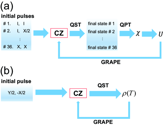
Figure 1: Schematic diagrams of two data-driven GRAPE protocols implemented in our experiment. These two protocols are designed under the optimization of (a) the fitted gate operator $U$ and (b) an output density matrix $\rho(T)$, respectively.

II Data-Drive GRAPE Protocol I

In this section, we provide the theoretical description of our first data-driven GRAPE protocol for the realization of the CZ gate, similar to the design in Ref. [24]. A schematic diagram of this protocol is shown in Fig. 1(a). The Hamiltonian of a two-qubit ($A$ and $B$) system is written as

$$H_{0}=H_{A}+H_{B}+H_{\mathrm{int}},$$ (1)

where $H_{A}$ and $H_{B}$ are two single-qubit Hamiltonians, and $H_{\mathrm{int}}$ is the interaction between two qubits. Since our CZ gate is assisted by the second excited state of one qubit [9], a three-level model is considered in the single-qubit Hamiltonian,

$$H_{i=A,B}=\omega_{i}|1_{i}\rangle\langle 1_{i}|+\left(2\omega_{i}+\Delta_{i})\right|2_{i}\rangle\langle 2_{i}|.$$ (2)

For each qubit ($i=A,B$), $\omega_{i}$ and $\Delta_{i}$ are its resonant frequency and anharmonicity parameter, respectively. The reduced Planck constant $\hbar$ is set to be unity throughout this paper. In our experiment, the frequency shift is $\delta\omega/2\pi=(\omega_{A}-\omega_{B})/2\pi=539.0$ MHz and the two anharmonicity parameters are $\Delta_{A}/2\pi=-242.1$ MHz and $\Delta_{B}/2\pi=-258.8$ MHz. The interaction term is written as

$$H_{\mathrm{int}}=g(a_{A}^{\dagger}a_{B}+a_{A}a_{B}^{\dagger}),$$ (3)

where $a_{i=A,B}=\sum_{j=1}^{2}\sqrt{j}|(j-1)_{i}\rangle\langle j_{i}|$ and $a_{i=A,B}^{\dagger}=\sum_{j=0}^{1}\sqrt{j+1}|(j+1)_{i}\rangle\langle j_{i}|$ are the lowering and raising operators, respectively. In our experiment, the coupling strength is $g/2\pi=9.1$ MHz.

Due to the condition of a weak interaction ($g\ll\delta\omega,|\Delta_{A}|,|\Delta_{B}|$), the population exchange between two qubits is usually negligible, but a $Z$-control pulse can tune the energy levels and create an inter-qubit resonance. In our experiment, the $Z$-pulse $\mu_{A}(t)$ is applied to qubit $A$, which gives rise to

$$H_{\mathrm{ext}}(t)=\mu_{A}(t)n_{A},$$ (4)

with the number operator $n_{A}=\sum_{j=0}^{2}j|j_{A}\rangle\langle j_{A}|$. The coupled Hamiltonian, $H_{c}(t)=H_{0}(g)+H_{\mathrm{ext}}(t)$, creates the resonance between $|2_{A}0_{B}\rangle$ and $|1_{A}1_{B}\rangle$ under the pulse amplitude, $\mu_{A}(t)=\mu_{A;r}=-(\delta\omega+\Delta_{A})$. For conciseness, the notation of an arbitrary state, $|j_{A}j^{\prime}_{B}\rangle$, is abbreviated to $|jj^{\prime}\rangle$ where the first and second state indices refer to qubits $A$ and $B$, respectively.

In a simplified treatment, the Hilbert space is reduced to $\{|00\rangle,|10\rangle,|01\rangle,|11\rangle,|20\rangle\}$, while the coupling only exists between $|11\rangle$ and $|20\rangle$ with the strength $\sqrt{2}g$. If the energy difference between these two states is precisely tuned to zero ($\mu_{A}(0<t<T)=\mu_{A;r}$) and the operation time is equal to one period of the Rabi oscillation ($T=\pi/\sqrt{2}g$), a $\pi$-phase is generated for $|11\rangle$ and $|20\rangle$. In the five-state Hilbert space, the time evolution operator is given by

$$U_{c} = |00\rangle\langle 00|+e^{-i\phi_{A}}|10\rangle\langle 10|+e^{-i\phi_{B}}|01\rangle\langle 01|$$ (5)

$$-e^{-i(\phi_{A}+\phi_{B})}|11\rangle\langle 11|-e^{-i(\phi_{A}+\phi_{B})}|20\rangle\langle 20|,$$

where $\phi_{A}=\int_{0}^{T}[\omega_{A}+\mu_{A}(t)]dt$ and $\phi_{B}=\omega_{B}T$ are the dynamic phases associated with the first excited states of qubits $A$ and $B$, respectively. In experiment, these two dynamic phases can be measured and compensated [9], which is described by an auxiliary operator,

$$U^{\dagger}_{d} = |00\rangle\langle 00|+e^{i\phi_{A}}|10\rangle\langle 10|+e^{i\phi_{B}}|01\rangle\langle 01|$$ (6)

$$+e^{i(\phi_{A}+\phi_{B})}|11\rangle\langle 11|+e^{i(\phi_{A}+\phi_{B})}|20\rangle\langle 20|.$$

This operator can be viewed as a reversed time evolution over a decoupled Hamiltonian, $H_{d}(t)=H_{0}(g=0)+H_{\mathrm{ext}}(t)$. The combination of these two operations gives rise to the ideal CZ gate,

$$U_{\mathrm{CZ}} = U^{\dagger}_{d}U_{c}=|00\rangle\langle 00|+|10\rangle\langle 10|+$$ (7)

$$|01\rangle\langle 01|-|11\rangle\langle 11|-|20\rangle\langle 20|.$$

Note that a standard CZ gate does not involve the evolution of state $|20\rangle$, which is satisfied in our treatment if the initial quantum state is inside the subspace of $\{|00\rangle,|10\rangle,|01\rangle,|11\rangle\}$.

The experimental realization of an ideal square-shaped pulse is difficult due to the bandwidth limitation of the waveform generator. The residual errors in the control line in general cause that the input pulse experienced by the qubit sample deviates from its theoretical design. In literature, various approaches have been designed to modify the pulse shape and improve the gate fidelity [8, 11, 9]. In this paper, we apply a data-driven GRAPE method as follows. The operation time $T$ is discretized into $M$ segments, each with the same length $\tau=T/M$. The $Z$-control pulse becomes an amplitude sequence, i.e., $\mu_{A}(t)\Rightarrow\{\mu_{A;1},\mu_{A;2},\cdots,\mu_{A;M}\}$, which leads to $H_{c}(t)\Rightarrow\{H_{c;1},H_{c;2},\cdots,H_{c;M}\}$ and $H_{d}(t)\Rightarrow\{H_{d;1},H_{d;2},\cdots,H_{d;M}\}$. The two Hamiltonians are given by $H_{c;m}=H_{0}(g)+H_{\mathrm{ext}}(\mu_{A;m})$ and $H_{d;m}=H_{0}(g=0)+H_{\mathrm{ext}}(\mu_{A;m})$ at each $m$-th time segment. The two time evolution operators in Eqs. (5) and (6) are expanded into

$$U_{c} = U_{c;M}U_{c;M-1}\cdots U_{c;2}U_{c;1},$$ (8)

$$U^{\dagger}_{d} = U^{\dagger}_{d;1}U^{\dagger}_{d;2}\cdots U^{\dagger}_{d;M-1}U^{\dagger}_{d;M},$$ (9)

with $U_{c;m}=\exp(-iH_{c;m}\tau)$ and $U^{\dagger}_{d;m}=\exp(iH_{d;m}\tau)$.

Next we introduce an objective function,

$${\mathcal{F}}_{U}=\|U^{\dagger}_{d}U_{c}-U_{\mathrm{CZ}}\|^{2},$$ (10)

where the Euclidean norm of matrix $R$ is defined as $\|R\|=\sqrt{\mathrm{Tr}\{R^{{\dagger}}R\}}$. The discretization of the $Z$-control pulse determines that this function is fully dependent on the pulse sequence, i.e., $\mathcal{F}_{U}\equiv\mathcal{F}_{U}(\mu_{A;1},\mu_{A;2},\cdots,\mu_{A;M})$. For each $m$-th amplitude, the gradient of the objective function, $k_{U,m}=\partial\mathcal{F}_{U}/\partial\mu_{A;m}$, is given by

$$k_{U,m} = -2\mathrm{Re}\mathrm{Tr}\left\{U_{\mathrm{CZ}}U_{d}^{{\dagger}}\frac{\partial U_{c}}{\partial\mu_{A;m}}\right\}-2\mathrm{Re}\mathrm{Tr}\left\{U_{c}^{{\dagger}}\frac{\partial U_{d}}{\partial\mu_{A;m}}U_{\mathrm{CZ}}\right\},$$ (11)

where Re stands for the real part. By neglecting the commutation terms, the two partial derivatives are approximated as $\partial U_{c}/\partial\mu_{A;m}\approx-i\tau U_{c}Q_{c;m}$ and $\partial U_{d}/\partial\mu_{A;m}\approx-i\tau U_{d}Q_{d;m}$. Here we introduce two abbreviations, $Q_{c;m}=R^{\dagger}_{c;m}n_{A}R_{c;m}$ with $R_{c;m}=U_{c;m}U_{c;m-1}\cdots U_{c;1}$ and $Q_{d;m}=R^{\dagger}_{d;m}n_{A}R_{d;m}$ with $R_{d;m}=U_{d;m}U_{d;m-1}\cdots U_{d;1}$. The gradient in Eq. (11) is simplified to be

$$k_{U;m} \approx -2\tau\mathrm{Im}\mathrm{Tr}\{U_{\mathrm{CZ}}U_{d}^{{\dagger}}U_{c}Q_{c;m}\}-2\tau\mathrm{Im}\mathrm{Tr}\{U_{\mathrm{CZ}}U^{\dagger}_{c}U_{d}Q_{d;m}\},$$ (12)

where Im stands for the imaginary part.

The optimization of the CZ gate is given by the minimization of the objective function, which leads to an array of $M$ equations,

$$k_{U;m=1,2\cdots,M}=0.$$ (13)

However, this optimization condition is nearly impossible to be solved analytically and we apply the GRAPE method based on an iteration approach [24]. The protocol begins with an initial guess of the pulse sequence, ${\bm{\mu}}^{(0)}_{A}=\{\mu^{(0)}_{A;1},\cdots,\mu^{(0)}_{A;M}\}$. At each $l$-th step, we numerically calculate the gradient sequence, ${\bm{k}}^{(l)}=\{k^{(l)}_{1},\cdots,k^{(l)}_{M}\}$, and update the pulse sequence using a linear propagation,

$$\mu^{(l+1)}_{A;m}=\mu^{(l)}_{A;m}+\alpha k^{(l)}_{m},$$ (14)

where the learning rate $\alpha$ is an empirical constant. Through a series of iteration steps,

$$\cdots\rightarrow{\bm{\mu}}^{(l)}\rightarrow{\bm{k}}^{(l)}\rightarrow{\bm{\mu}}^{(l+1)}\rightarrow\cdots,$$

the gradient sequence approaches very small values (${\bm{k}}^{(l)}\approx 0$) and the pulse sequence is nearly invariant (${\bm{\mu}}^{(l+1)}_{A}\approx{\bm{\mu}}^{(l)}_{A}$). The optimization of the $Z$-control pulse is thus achieved. There are a few issues to be emphasized in this protocol: (1) Equation (14) is a simple updating strategy and more complicated ones are allowed. (2) The high-dimensional optimization is highly dependent on the initial guess. (3) Although the optimized pulse sequence can be obtained through a pure numerical computation, the experimental deviation in the pulse shape requires a data-driven approach to minimize the influence of the residual errors in the control line [24]. Accordingly, the gradient in Eq. (12) is replaced by

$$k^{(l)}_{U;m} \approx -2\tau\mathrm{Im}\mathrm{Tr}\{U_{\mathrm{CZ}}U^{(l)}_{\mathrm{exp}}Q^{(l)}_{c;m}\}-2\tau\mathrm{Im}\mathrm{Tr}\{U_{\mathrm{CZ}}(U^{(l)}_{\mathrm{exp}})^{\dagger}Q^{(l)}_{d;m}\}.$$ (15)

Here $Q^{(l)}_{c;m}$ and $Q^{(l)}_{d;m}$ are numerically calculated using the input ${\bm{\mu}}^{(l)}_{A}$-sequence, while $U^{(l)}_{\mathrm{exp}}=(U^{(l)}_{d})^{\dagger}U^{(l)}_{c}$ is experimentally estimated.

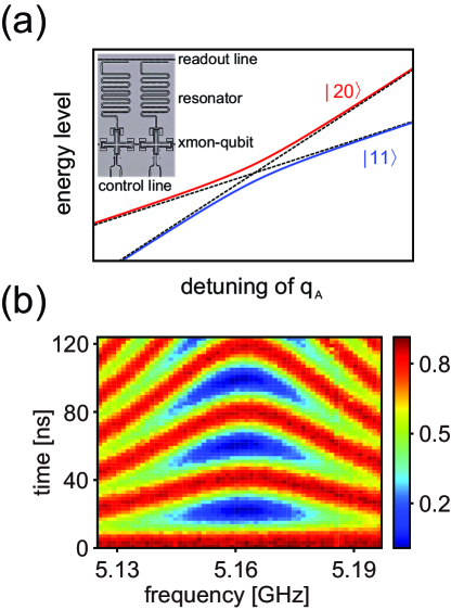
Figure 2: (a) The blue and red solid lines present an avoided crossing for the states $|11\rangle$ and $|20\rangle$, while the two crossed dashed lines denote energy levels with a zero coupling. Inset is an optical micrograph composed of two coupled X-shaped transmon qubits. (b) The probability $P_{11}$ of the state $|11\rangle$ versus the target qubit frequency and the swap time.

III Experimental Implementation of Protocol I

III.1 Setup

In the inset of Fig. 2(a), we show an image of two coupled X-shaped transmon qubits [28, 29], in which four arms of each qubit are connected to the readout resonator, the $XY$-control line, the $Z$-control line, and the neighboring qubit. Each qubit is biased at an operation frequency through its $Z$-control line. In our experiment, the two qubits are initially biased at $\omega_{A}/2\pi=5.458$ GHz and $\omega_{B}/2\pi=4.919$ GHz, while their qubit anharmonicities are $\Delta_{A}/2\pi=-242.1$ MHz and $\Delta_{B}/2\pi=-258.8$ MHz. In our CZ gate operation, the fast tuning of $\omega_{A}$ is implemented by an external pulse $\mu_{A}(t)$ through the $Z$-control line. At designated operation points, the relaxation times are $T_{A;1}=15.3~{}\mu$s and $T_{B;1}=27.9~{}\mu$s and the pure dephasing times are $T_{A;\phi}=13.8~{}\mu$s and $T_{B;\phi}=42.7~{}\mu$s. Microwave drive pulses are transported through the $XY$-control lines to control the single-qubit gate. In the qubit state measurement, a measure pulse is transported through the readout line, interacts with read-out resonators, and outputs a read-out signal for the later amplification and data-collection. The frequencies of two read-out resonators are $\omega_{A;r}/2\pi=6.462$ GHz and $\omega_{B;r}/2\pi=6.443$ GHz. The read-out fidelities of the ground state $|0\rangle$ and the excited state $|1\rangle$ are $F_{A}^{0}=97.8\%$ and $F_{A}^{1}=93.7\%$ for qubit $A$, and $F_{B}^{0}=95.2\%$ and $F_{B}^{1}=90.4\%$ for qubit $B$. The $Z$ line cross talk are simultaneously calibrated and corrected, with residue coefficients below $0.2\%$.

The two-qubit CZ gate mainly depends on the $Z$-control pulse, which could be distorted with rising or falling edges due to a filtering effect. The $Z$ line response is calibrated and corrected, with a method similar to that in Ref. [2]. The deconvolution parameters are thereafter embedded in the underlying program to automatically correct imperfections of the $Z$ line response. To verify this correction, we measure a swap spectrum between the $|11\rangle$ and $|20\rangle$ states. Figure 1(b) shows the measured probability $P_{11}$ as a result of the detuning time and the detuned frequency of qubit $A$. A typical chevron pattern is observed, which confirms the reliability of the $Z$ line correction. This chevron pattern also enables precise extraction of two experimental parameters, the coupling strength $g$ and the resonant frequency between $|11\rangle$ and $|20\rangle$ states.

III.2 Experimental results

In this subsection, we present our experimental result of an optimal CZ gate pulse under the data-driven GRAPE protocol I. The initial guess $\mu^{(0)}_{A}(0\leq t\leq T)$ is selected to follow a flattop waveform as

$$\mu^{(0)}_{A}(t)=\frac{\Gamma}{2}\left[\mathrm{Erf}\left(4\sqrt{\ln{2}}(t\sigma^{-1}-1)\right)-\mathrm{Erf}\left(4\sqrt{\ln{2}}(t\sigma^{-1}+1-T\sigma^{-1})\right)\right],$$ (16)

where $\mathrm{Erf}$ denotes the error function. To demonstrate the capability of the GRAPE protocol, we manually deviate the amplitude and the operation time away from their ideal values under a square pulse shape. In particular, the parameters in our experiment are set as $\Gamma/2\pi=-290.6$ MHz, $T=50$ ns, and $\sigma=4$ ns.

To quantify the fidelity of the initial CZ gate, we perform a QPT measurement. As shown in Fig. 1(a), each qubit ($A$ or $B$) is prepared at an initial state from the set of $\{{|0\rangle,|1\rangle,(|0\rangle\pm|1\rangle)/\sqrt{2},(|0\rangle\pm i|1\rangle)/\sqrt{2}}\}$, which is created by a ground state qubit subject to the pulses of $\{I,X,\pm Y/2,\mp X/2\}$. The total 36 initial states are inspected in a single QPT measurement. For each initial state, its final state after the CZ gate operation is measured by the QST and calibrated with the read-out fidelities to eliminate the state preparation and measurement errors [9]. If the initial density matrix is $\rho(0)$, the output counterpart $\rho^{(0)}(T)$ is in general expanded into

$$\rho^{(0)}(T)=\sum_{mn}\chi^{(0)}_{mn}\tilde{E}_{m}\rho(0)\tilde{E}_{n}^{\dagger},$$ (17)

where $\{\tilde{E}_{m}\}$ is a complete set of two-qubit operators. As a full description of the gate operation, the $\chi^{(0)}$-matrix ($\chi^{(0)}=\{\chi^{(0)}_{mn}\}$) is numerically determined using the QST data of $\rho^{(0)}(T)$ from all the 36 initial states. Then we calculate the process fidelity using $F(\chi^{(0)})=\mathrm{Tr}\{(\chi^{(0)})^{\dagger}\chi_{\mathrm{ideal}}\}$, where $\chi_{\mathrm{ideal}}$ is the ideal matrix [9]. As shown in Fig. 3(a), the initial flattop form $\mu^{(0)}_{A}(t)$ leads to the gate fidelity at $F(\chi^{(0)})=81.4\%$, which suggests an improvement necessary in the $Z$-control pulse.

To fulfill the GRAPE protocol I, we need to employ the gate operator $U^{(0)}_{\mathrm{exp}}$. In our experiment, the Powell method [30] is utilized to extract an estimation of $U^{(0)}_{\mathrm{exp}}$ from the $\chi^{(0)}$-matrix. The fidelity of the initial gate operator, $F(U^{(0)}_{\mathrm{exp}})=\mathrm{Tr}\{(U^{(0)}_{\mathrm{exp}})^{\dagger}U_{\mathrm{CZ}}\}/4$, is estimated at 88.2%. Here we must emphasize that the operator $U_{\mathrm{exp}}$ is less reliable than the process matrix $\chi$ due to a possible overfitting of the former in a smaller space. However, an analytical relation between $\chi$ and $\mu_{A}(t)$ is extremely difficult to be extracted so that a direct optimization of the $\chi$-matrix is highly inefficient. We then use the estimated gate operator $U^{(0)}_{\mathrm{exp}}$ to calculate the gradient sequence ${\bm{k}}^{(1)}_{U}=\{k^{(1)}_{U;1},\cdots,k^{(1)}_{U;M}\}$ and the pulse sequence ${\bm{\mu}}^{(1)}_{A}=\{\mu^{(1)}_{A;1},\cdots,\mu^{(1)}_{A;M}\}$. The above iteration procedure is repeated upto convergence. At each $l$-th iteration step, the time step of discretization is set to be $\tau=0.5$ ns considering the resolution limit of our arbitrary waveform generator (AWG) [31]. The learning rate is empirically set to be $\alpha=0.03$ GHz². After the experimental measurement of the $\chi^{(l)}$-matrix and the numerical estimation of $U^{(l)}_{\mathrm{exp}}$, the discrete pulse sequence ${\bm{\mu}}^{(l+1)}_{A}$ is calculated by Eq. (15) and interpolated to be a continuous function $\mu^{(l+1)}_{A}(t)$, which is sent to the AWG for the $(l+1)$-th gate operation.

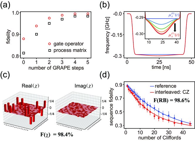
Figure 3: The experimental results of the data-driven GRAPE protocol I. (a) The fidelities of the process matrix $F(\chi^{(l)})$ (black squares) and the fitted gate operator $F(U^{(l)}_{\mathrm{exp}})$ (red circles) as functions of the iteration step $l$. (b) The pulse shape modification through the iteration procedure. The initial flattop waveform (blue) and the optimal pulse $\mu^{(5)}_{A}(t)$ (red) are shown. In the inset, the resonance region of six pulses ($\mu^{(0)}_{A}(t)\rightarrow\mu^{(5)}_{A}(t)$ from top to bottom) are enlarged. (c) The QPT measurement of the $\chi$-matrix subject to the optimal CZ gate. (d) The sequence fidelities (reference in blue and interleaved in red) versus the number of the Clifford gates, where the CZ gate is implemented by the optimal $Z$ pulse. For each result, an error bar of the standard deviation is shown together with the average value.

The behavior of the iteration procedure is summarized in Figs. 3(a)-(b). A bump is created in the resonance region of $\mu_{A}(t)$ where the pulse amplitude is enhanced to compensate an insufficient phase accumulation in $|11\rangle$. In the first three steps of the iteration procedure, the gate fidelity is quickly improved from $F(\chi^{(0)})=81.4\%$ to $F(\chi^{(3)})=97.0\%$, in parallel with $F(U^{(0)}_{\mathrm{exp}})=88.2\%\rightarrow F(U^{(3)}_{\mathrm{exp}})=99.3\%$. Afterwards, the shape modification of the $Z$-control pulse slows down and the same for the improvement of the fidelities. The pulse $\mu^{(5)}_{A}(t)$ after five iteration steps leads to the gate fidelity at $F(\chi^{(5)})=98.4\%$ and the fitted operator fidelity at $F(U^{(5)}_{\mathrm{exp}})=99.9\%$. Notice that $F(U^{(l)}_{\mathrm{exp}})$ is consistently larger than $F(\chi^{(l)})$ due to the overfitting of $U^{(l)}_{\mathrm{exp}}$.

For simplicity, we terminate the iteration procedure and choose $\mu^{(5)}_{A}(t)$ to be our optimal pulse of the CZ gate. Figure 3(c) presents a detailed structure of the $\chi^{(5)}$-matrix. Through an expansion over $\{\tilde{E}_{m}=\tilde{E}_{A}\tilde{E}_{B}\}$ with $\tilde{E}_{A},\tilde{E}_{B}\!\in\!\{I,X,Y,Z\}$, the real part of the $\chi^{(5)}$-matrix is located at the four corners and the imaginary part of the $\chi^{(5)}$-matrix is close to zero, in an excellent agreement with the ideal result. Next we implement a RB measurement to quantify the gate fidelity alternatively [2]. Two qubits are prepared at $|00\rangle$ and driven by a sequence of $n$ random Clifford gates, and the ground state population ($P_{00}$) is measured after a recovery gate. For such a reference sequence, an interleaved one is formed by adding a CZ gate after each Clifford gate. The average populations $\bar{P}_{00}(n)$ and $\bar{P}^{\prime}_{00}(n)$ over 30 reference and interleaved sequences respectively are also plotted in Fig. 3(d). Both populations are fitted by $f(n)=ap^{n}+b$ with $f(n)=\bar{P}_{00}(n)$ and $\bar{P}^{\prime}_{00}(n)$ [2]. The fidelity of the interleaved CZ gate is defined as $F(\mathrm{RB})\!=\!1\!-\!(3/4)(1\!-\!p_{\mathrm{CZ}}/p_{\mathrm{ref}})$, where the fitting parameters $p_{\mathrm{ref}}$ and $p_{\mathrm{CZ}}$ refer to the reference and interleaved sequences, respectively [2]. For our optimal pulse $\mu^{(5)}(t)$, the RB fidelity is estimated at $F(\mathrm{RB}|\mu^{(5)}(t))=98.6\%$.

IV Data-Drive GRAPE Protocol II

In our first data-driven GRAPE protocol, the objective function is designed to optimize the CZ gate operator $U_{\mathrm{exp}}$, which is indirectly obtained by the Powell algorithm acting on the $\chi$-matrix. This approach requires the QPT measurement over 36 initial states at each iteration step, leading to a relatively slow optimization process. In this section, we design an alternative protocol based on the optimization of a target density matrix, as shown by the schematic diagram in Fig. 1(b).

With a weak quantum dissipation, the time evolution of the density matrix $\rho(t)$ is described by the Lindbald master equation as [32]

$$\dot{\rho}(t) = -i[H(t),\rho(t)]$$ (18)

$$+\sum_{i=A,B}\sum_{j=1}^{2}\left(L_{i;j}\rho(t)L_{i;j}^{\dagger}-\frac{1}{2}\{\rho(t),L_{i;j}^{\dagger}L_{i;j}\}\right),$$

where $L_{i=A,B;j=1,2}$ are the Lindblad operators. For each qubit ($i=A,B$), the Lindblad operators, $L_{i;1}$ and $L_{i;2}$, refer to the relaxation and the pure dephasing, respectively. In the Liouville superspace [32], Eq. (18) is formally rewritten as

$$\dot{\rho}(t)=-i\mathcal{L}(t)\rho(t),$$ (19)

where $\mathcal{L}(t)$ is the Liouville superoperator including the influence of both the system Hamiltonian and the bath-induced dissipation (see Appendix A). Since the realization of the CZ gate involves the coupled Hamiltonian $H_{c}(t)=H_{0}(g)+H_{\mathrm{ext}}(t)$ and the decoupled one $H_{d}(t)=H_{0}(g=0)+H_{\mathrm{ext}}(t)$, two Liouville superoperators are needed in our derivation, i.e., $H_{c}(t)\rightarrow\mathcal{L}_{c}(t)$ and $H_{d}(t)\rightarrow\mathcal{L}_{d}(t)$. However, the auxiliary time evolution over $H_{d}(t)$ is performed by the phase measurement so that the dissipation is ignored.

Following the approach in Sec. II, the operation time $T$ is discretized into $M$ segments. The two Liouville superoperators become $\mathcal{L}_{c}(t)\Rightarrow\{\mathcal{L}_{c;1},\mathcal{L}_{c;2},\cdots,\mathcal{L}_{c;M}\}$ and $\mathcal{L}_{d}(t)\Rightarrow\{\mathcal{L}_{d;1},\mathcal{L}_{d;2},\cdots,\mathcal{L}_{d;M}\}$, where the terms at each $m$-th segment are dependent on the external pulse $\mu_{A;m}$, i.e., $\mathcal{L}_{c;m}\equiv\mathcal{L}_{c;m}(\mu_{A;m})$ and $\mathcal{L}_{d;m}\equiv\mathcal{L}_{d;m}(\mu_{A;m})$. The partial time evolution superoperators in the Liouville space are defined as $\mathcal{U}_{c;m}=\exp(-i\mathcal{L}_{c;m}\tau)$ and $\mathcal{U}_{d;m}=\exp(-i\mathcal{L}_{d;m}\tau)$. For a given initial state $\rho(0)$, the output density matrix at time $T$ is written as $\rho(T)=\mathcal{U}^{-1}_{d}\mathcal{U}_{c}\rho(0)$ with

$$\mathcal{U}_{c} = \mathcal{U}_{c;M}\mathcal{U}_{c;M-1}\cdots\mathcal{U}_{c;2}\mathcal{U}_{c;1},$$ (20)

$$\mathcal{U}^{-1}_{d} = \mathcal{U}^{-1}_{d;1}\mathcal{U}^{-1}_{d;2}\cdots\mathcal{U}^{-1}_{d;M-1}\mathcal{U}^{-1}_{d;M}.$$ (21)

The reliability of the CZ gate can be described by the deviation between the real output state $\rho(T)$ and the ideal one $\rho_{\mathrm{ideal}}$, which leads to an objective function,

$$\mathcal{F}_{\rho} = \|\rho(T)-\rho_{\mathrm{ideal}}\|^{2}$$ (22)

$$\approx 2-2\mathrm{Tr}\{\rho(T)\rho_{\mathrm{ideal}}\}.$$

The optimization criterion is given by the zero gradients, $k_{\rho;m=1,\cdots,M}=\partial\mathcal{F}_{\rho}/\partial\mu_{A;m}=0$, achieved by the GRAPE approach. With an initial guess ${\bm{\mu}}^{(0)}_{A}(t)$, we also update the external field using a linear propagation over gradients, i.e., $\mu^{(l+1)}_{A;m}=\mu^{(l)}_{A;m}+\alpha k^{(l)}_{\rho;m}$. This iteration is finished when the pulse sequence is converged by ${\bm{\mu}}^{(l+1)}_{A}\approx{\bm{\mu}}^{(l)}_{A}$ and ${\bm{k}}^{(l)}_{\rho}\approx 0$. In detail, each gradient is given by

$$k^{(l)}_{\rho;m} \approx 2i\tau\rho^{\dagger}_{\mathrm{ideal}}\mathcal{Q}^{(l)}_{c;m}\rho^{(l)}_{\mathrm{exp}}(T)-2i\tau\rho^{\dagger}_{\mathrm{ideal}}\mathcal{Q}^{(l)}_{d;m}\rho^{(l)}_{\mathrm{exp}}(T),$$ (23)

with $\mathcal{Q}^{(l)}_{c;m}=(\mathcal{R}^{(l)}_{c;m})^{-1}\mathcal{P}_{A}\mathcal{R}^{(l)}_{c;m}$ and $\mathcal{Q}^{(l)}_{d;m}=(\mathcal{R}^{(l)}_{d;m})^{-1}\mathcal{P}_{A}\mathcal{R}^{(l)}_{d;m}$. Here $\mathcal{P}_{A}=[n_{A},\cdots]$ denotes the commutator over the number operator $n_{A}$, and the two partial time evolution superoperators are $\mathcal{R}^{(l)}_{c;m}=(\mathcal{U}^{(l)}_{c;m+1})^{-1}\cdots(\mathcal{U}^{(l)}_{c;M})^{-1}\mathcal{U}^{(l)}_{d}$ and $\mathcal{R}^{(l)}_{d;m}=\mathcal{U}^{(l)}_{d;m}\cdots\mathcal{U}^{(l)}_{d;1}$. In practice, $\mathcal{Q}^{(l)}_{c;m}$ and $\mathcal{Q}^{(l)}_{d;m}$ are numerically calculated using the $l$-th pulse sequence ${\bm{\mu}}^{(l)}$, while the output density matrix $\rho^{(l)}_{\mathrm{exp}}(T)$ are experimentally determined by the QST measurement. An average over multiple output states can improve the applicability of this GRAPE protocol.

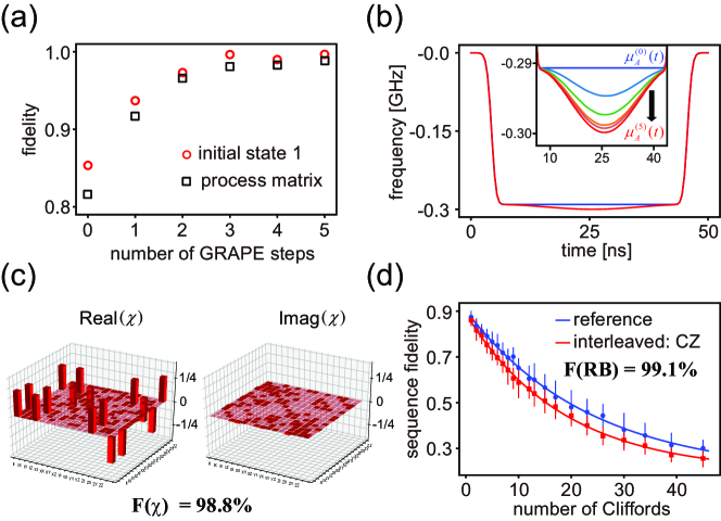
Figure 4: The experimental results of the data-driven GRAPE protocol II. (a) The fidelities of an output density matrix $F(\rho^{(l)}_{\mathrm{exp}}(T)|\varphi_{1}(0))$ (red circles) and the process matrix $F(\chi^{(l)})$ (black squares) as functions of the iteration step $l$. (b) The pulse shape modification through the iteration procedure. (c) The QPT measurement of the $\chi$-matrix subject to the optimal CZ gate. (d) The sequence fidelities under the optimal $Z$ pulse in the RB measurement. The legends in (b)-(d) are the same as those in Figs. 3(b)-(d).

V Experimental Implementation of Protocol II

In this section, we present the experimental result of an optimal CZ gate under the data-driven GRAPE protocol II. The same flattop waveform with the same parameters as in Sec. III.2 is selected for the initial guess $\mu^{(0)}_{A}(t)$. Four specific initial states, $\varphi_{1,2}(0)=(|0\rangle\pm|1\rangle)\otimes(|0\rangle\pm i|1\rangle)/2$ and $\varphi_{3,4}(0)=(|0\rangle\pm i|1\rangle)\otimes(|0\rangle\pm|1\rangle)/2$, are considered in the optimization procedure. These initial states are created by the pulses of $\{\pm Y/2,\mp X/2\}$ and $\{\mp X/2,\pm Y/2\}$ applying to the two ground-state qubits. For the initial $Z$-control pulse, the fidelities of the four output density matrices, $F(\rho^{(0)}_{\mathrm{exp}}(T))=\mathrm{Tr}\{\rho^{(0)}_{\mathrm{exp}}(T)\rho_{\mathrm{ideal}}\}$, are in the range of $81.5\%\sim 85.3\%$, consistent with the gate fidelity $F(\chi^{(0)})=81.4\%$. For each output density matrix, we calculate the gradient sequence ${\bm{k}}^{(1)}_{\rho}$ using Eq. (23) and obtain an updated pulse sequence ${\bm{\mu}}^{(1)}_{A}$. The time step is $\tau=0.5$ ns and the learning rate is $\alpha=0.1$ GHz². The average of four pulse sequences are interpolated to generate a continuous form $\mu^{(1)}_{A}(t)$ for the subsequent gate operation. This procedure is then repeated until being terminated at $\mu^{(5)}_{A}(t)$.

The evolution of the iteration process is shown in Figs. 4(a)-(b). The CZ gate is quickly improved in the first three steps and then gradually approaches an optimal result. For example, the fidelity of the output density matrix evolved from $\varphi_{1}(0)$ becomes $F(\rho^{(3)}_{\mathrm{exp}}(T))=99.6\%$ after three iteration steps and is stabilized above 99% thereafter (see Fig. 4(a)). For clarity, we perform the QPT measurement for each $l$-th $Z$-control pulse $\mu^{(l)}_{A}(t)$ despite the fact the $\chi$-matrix is unnecessary in the protocol II. As shown in Fig. 4(b), the gate fidelity is improved as $F(\chi^{(0)})=81.4\%\rightarrow F(\chi^{(3)})=98.0\%\rightarrow F(\chi^{(5)})=98.8\%$. Similar to the behavior in the protocol I, the shape modification mainly occurs in the resonance region of the $Z$-control pulse, in which an additional bump is created for the sufficient phase accumulation.

The pulse $\mu^{(5)}_{A}(t)$ obtained after five iteration steps is treated as the second optimal $Z$-control pulse of the CZ gate. In Fig. 4(c), we present the corresponding structure of the $\chi^{(5)}$-matrix, which agrees excellently with an ideal one. In Fig. 4(d), we present the result of the RB measurement using $\mu^{(5)}_{A}(t)$ as the interleaved CZ gate. Following the data analysis method in Sec. III, we obtain the RB fidelity of the second optimal CZ gate at $F(\mathrm{RB}|\mu^{(5)}_{A}(t))=99.1\%$, in comparable to the result from the GRAPE protocol I.

VI Summary

In this paper, we experimentally implement the optimization of the two-qubit CZ gate based on two different data-driven GRAPE protocols. These two protocols are designed to minimize two different objective functions based on the fitted gate operator and a target output density matrix, respectively. Following a feedback-control mechanism, the key step in each protocol utilizes mixed information of the input $Z$-control pulse and the experimental measurements (the QPT and the QST) to numerically calculate a gradient sequence, which leads to the subsequent $Z$-control pulse. A well fabricated quantum device of superconducting X-shaped transmon qubits is used for the realization of these two GRAPE protocols. For both protocols, we quickly obtain the optimal $Z$-control pulses around 5 iteration steps. The resulted two CZ gates are confirmed to yield high fidelities in the QPT measurement ($98.4\%$ and $98.8\%$) and the RB measurement ($98.6\%$ and $99.1\%$).

The main advantage of the GRAPE algorithm is its efficiency in the convergence speed, especially by optimizing the density matrices in the second protocol. In the previous RB-based Nelder-Mead algorithm, the pulse sequence with different number of Clifford gates should be explored and each case requires a large number of random sequences, despite that only the ground state population is be measured. Nevertheless, the search speed of the Nedler-Mead algorithm is intrinsically slower than that of the GRAPE algorithm. As a result, the Nedler-Mead is more suitable for the parameter optimization under a fixed waveform while the GRAPE for a pulse sequence over a fixed operation time. In general, there always exist many, sometime a huge number of, possibilities in the problem of high-dimensional optimization. Our experimental results show that the gate fidelities from two different data-driven GRAPE protocols are close to each other and comparable with those from previous RB-based Nelder-Mead experiments. Overall, various algorithms compose a comprehensive strategy for the optimization of the CZ gate.

Appendix A Liouville Superoperators

In this Appendix, we summarize the Liouville superoperators in the Lindblad equation. The superoperator for the commutator of the system Hamiltonian $H(t)$ is

$$[\mathcal{L}_{\mathrm{sys}}(t)]_{k_{1}l_{1},k_{2}l_{2}}=[H(t)]_{k_{1},k_{2}}\delta_{l_{1},l_{2}}-[H(t)]_{l_{2},l_{1}}\delta_{k_{1},k_{2}},$$ (24)

For each qubit, the superoperator for the population relaxation part is

$$[\mathcal{L}_{\mathrm{relax}}]_{k_{1}l_{1},k_{2}l_{2}}=\frac{i}{T_{1}}\left[\sqrt{k_{2}l_{2}}\delta_{k_{1}+1,k_{2}}\delta_{l_{1}+1,l_{2}}-\frac{1}{2}(k_{1}+l_{1})\delta_{k_{1},k_{2}}\delta_{l_{1},l_{2}}\right],$$ (25)

and the superoperator for the pure dephasing part is

$$[\mathcal{L}_{\mathrm{deph}}]_{k_{1}l_{1},k_{2}l_{2}}=-\frac{i}{T_{\phi}}(k_{1}-l_{1})^{2}\delta_{k_{1},k_{2}}\delta_{l_{1},l_{2}}.$$ (26)

References

- [1] M. A. Nielsen and I. Chuang, Quantum Computation and Quantum Information, Cambridge University Press, Cambridge, England (2010).
- [2] R. Barends, J. Kelly, A. Megrant, A. Veitia, D. Sank, E. Jeffrey, T. C. White, J. Mutus, A. G. Fowler, B. Campbell, Y. Chen, Z. Chen, B. Chiaro, A. Dunsworth, C. Neill, P. J. J. O’Malley, P. Roushan, A. Vainsencher, J. Wenner, A. N. Korotkov, A. N. Cleland, and J. M. Martinis, Superconducting quantum circuits at the surface code threshold for fault tolerance, Nature 508, 500 (2014).
- [3] R. Barends, C. M. Quintana, A. G. Petukhov, Y. Chen, D. Kafri, K. Kechedzhi et al., Diabatic Gates for Frequency-Tunable Superconducting Qubits, Phys. Rev. Lett. 123, 210501 (2019).
- [4] J. M. Chow, A. D. Córcoles, J. M. Gambetta, C. Rigetti, B. R. Johnson, J. A. Smolin, J. R. Rozen, G. A. Keefe, M. B. Rothwell, M. B. Ketchen, and M. Steffen, Simple All-Microwave Entangling Gate for Fixed-Frequency Superconducting Qubits, Phys. Rev. Lett. 107, 080502 (2011).
- [5] F. Yan, P. Krantz, Y. Sung, M. Kjaergaard, D. L. Campbell, T. P. Orlando, S. Gustavsson, and W. D. Oliver, Tunable Coupling Scheme for Implementing High-Fidelity Two-Qubit Gates, Phys. Rev. Appl. 10, 054062 (2018).
- [6] S. A. Caldwell, N. Didier, C. A. Ryan, E. A. Sete, A. Hudson, P. Karalekas et al., Parametrically Activated Entangling Gates Using Transmon Qubits, Phys. Rev. Appl. 10, 034050 (2018).
- [7] A. G. Fowler, M. Mariantoni, J. M. Martinis, A. N. Cleland, Surface codes: towards practical large-scale quantum computation, Phys. Rev. A 86, 032324 (2012).
- [8] J. Kelly, R. Barends, B. Campbell, Y. Chen, Z. Chen, B. Chiaro, A. Dunsworth, A. G. Fowler, I.-C. Hoi, E. Jeffrey, A. Megrant, J. Mutus, C. Neill, P. J. J. O’Malley, C. Quintana, P. Roushan, D. Sank, A. Vainsencher, J. Wenner, T. C. White, A. N. Cleland, and J. M. Martinis, Optimal Quantum Control Using Randomized Benchmarking, Phys. Rev. Lett. 112, 240504 (2014).
- [9] T. Wang, Z. Zhang, L. Xiang, Z. Jia, P. Duan, Z. Zong, Z. Sun, Z. Dong, J. Wu, Y. Yin, and G. Guo, Experimental Realization of a Fast Controlled-Z Gate via a Shortcut to Adiabaticity, Phys. Rev. Appl. 11, 034030 (2019).
- [10] L. DiCarlo, J. M. Chow, J. M. Gambetta, Lev S. Bishop, B. R. Johnson, D. I. Schuster, J. Majer, A. Blais, L. Frunzio, S. M. Girvin, and R. J. Schoelkopf, Demonstration of two-qubit algorithms with a superconducting quantum processor, Nature 460, 240 (2009).
- [11] John M. Martinis, Michael R. Geller, Fast adiabatic qubit gates using only control, Phys. Rev. A 90, 022307 (2014).
- [12] J. A. Nelder, R. Mead, A simplex method for function minimization, Computer Journal 7, 308 (1965).
- [13] J. M. Chow, J. M. Gambetta, L. Tornberg, Jens Koch, Lev S. Bishop, A. A. Houck, B. R. Johnson, L. Frunzio, S. M. Girvin, and R. J. Schoelkopf, Randomized Benchmarking and Process Tomography for Gate Errors in a Solid-State Qubit, Phys. Rev. Lett. 102, 090502 (2009).
- [14] J. M. Chow, J. M. Gambetta, L. Tornberg, Jens Koch, Lev S. Bishop, A. A. Houck, B. R. Johnson, L. Easwar Magesan, J. M. Gambetta, and Joseph Emerson, Scalable and Robust Randomized Benchmarking of Quantum Processes, Phys. Rev. Lett. 106, 180504 (2011).
- [15] Easwar Magesan, Jay M. Gambetta, B. R. Johnson, Colm A. Ryan, Jerry M. Chow, Seth T. Merkel, Marcus P. da Silva, George A. Keefe, Mary B. Rothwell, Thomas A. Ohki, Mark B. Ketchen, and M. Steffen, Efficient Measurement of Quantum Gate Error by Interleaved Randomized Benchmarking, Phys. Rev. Lett. 109, 080505 (2012).
- [16] N. Khaneja, T. Reiss, C. Kehlet, T. Schulte-Herbrüggen, and S. J. Glaser, Optimal control of coupled spin dynamics: design of NMR pulse sequences by gradient ascent algorithms, J. Magn. Reson. 172, 296 (2005).
- [17] F. Motzoi, J. M. Gambetta, S. T. Merkel, and F. K. Wilhelm, Optimal control methods for rapidly time-varying Hamiltonians, Phys. Rev. A 84, 022307 (2011)
- [18] R. S. Judson and H. Rabitz, Teaching Lasers to Control Molecules, Phys. Rev. Lett. 68, 1500 (1992)
- [19] C. Brif, R. Chakrabarti, and H. Rabitz, Control of quantum phenomena: past, present and future, New J. Phys. 12, 075008 (2010)
- [20] D. J. Egger and F. K. Wilhelm, Adaptive Hybrid Optimal Quantum Control for Imprecisely Characterized Systems, Phys. Rev. Lett. 112, 240503 (2014)
- [21] J. Li, X. Yang, X. Peng, C. Sun, Hybrid Quantum-Classical Approach to Quantum Optimal Control, Phys. Rev. Lett. 118, 150503 (2017).
- [22] D. Lu, K. Li, J. Li, H. Katiyar, A. J. Park, G. Feng, T. Xin, H. Li, G. L. Long, A. Brodutch, J. Baugh, B. Zeng and R. Laflamme, Enhancing quantum control by bootstrapping a quantum processor of 12 qubits, Npj Quantum Inf. 3, 45 (2017).
- [23] G. Feng, F. Cho, H. Katiyar, J. Li, D. Lu, J. Baugh, and R. Laflamme, Gradient-based closed-loop quantum optimal control in a solid-state two-qubit system, Phys. Rev. A 98, 052341 (2018).
- [24] R. B. Wu, B. Chu, D. H. Owens, H. Rabitz, Data-driven gradient algorithm for high-precision quantum control, Phys. Rev. A 97, 042122 (2018).
- [25] M. Mohseni, A. T. Rezakhani, and D. A. Lidar, Quantum-process tomography: Resource analysis of different strategies, Phys. Rev. A 77, 032322 (2008).
- [26] T. Yamamoto, M. Neeley, E. Lucero, R. C. Bialczak, J. Kelly, M. Lenander, Matteo Mariantoni, A. D. O’Connell, D. Sank, H. Wang, M. Weides, J. Wenner, Y. Yin, A. N. Cleland, and J. M. Martinis, Quantum process tomography of two-qubit controlled-Z and controlled-NOT gates using superconducting phase qubits, Phys. Rev. B 82, 184515 (2010).
- [27] Jerry M. Chow, Jay M. Gambetta, A. D. Córcoles, Seth T. Merkel, John A. Smolin, Chad Rigetti, S. Poletto, George A. Keefe, Mary B. Rothwell, J. R. Rozen, Mark B. Ketchen, and M. Steffen, Universal Quantum Gate Set Approaching Fault-Tolerant Thresholds with Superconducting Qubits, Phys. Rev. Lett. 109, 060501 (2012).
- [28] R. Barends, J. Kelly, A. Megrant, D. Sank, E. Jeffrey, Y. Chen, Y. Yin, B. Chiaro, J. Mutus, C. Neill, P. O’Malley, P. Roushan, J. Wenner, T. C. White, A. N. Cleland, John M. Martinis, Coherent Josephson Qubit Suitable for Scalable Quantum Integrated Circuits, Phys. Rev. Lett. 111, 080502 (2013).
- [29] T. Wang, Z. Zhang, L. Xiang, Z. Jia, P. Duan, W. Cai, Z. Gong, Z. Zong, M. Wu, J. Wu, Y. Yin, and G. Guo, The experimental realization of high-fidelity shortcut-to-adiabaticity quantum gates in a superconducting Xmon qubit, New J. of Phys. 20, 065003 (2018).
- [30] M. J. D. Powell, An efficient method for finding the minimum of a function of several variables without calculating derivatives, Computer Journal. 7, 155 (1964)
- [31] L. Xiang, Z. Zong, Z. Sun, Z. Zhan, Y. Fei, Z. Dong, C. Run, Z. Jia, P. Duan, J. Wu, Y. Yin, and G. Guo, Simultaneous Feedback and Feedforward Control and Its Application to Realize a Random Walk on the Bloch Sphere in an Xmon-Superconducting-Qubit System, Phys. Rev. Appl. 14, 014099 (2020).
- [32] S. Mukamel, Principles of Nonlinear Optical Spectroscopy, Oxford University Press, Oxford, England (1995).