On non-existence of continuous families of stationary nonlinear modes for a class of complex potentials

Abstract

There are two cases when the nonlinear Schrödinger equation (NLSE) with an external complex potential is well-known to support continuous families of localized stationary modes: the ${\cal PT}$-symmetric potentials and the Wadati potentials. Recently Y. Kominis and coauthors [Chaos, Solitons and Fractals, 118, 222-233 (2019)] have suggested that the continuous families can be also found in complex potentials of the form $W(x)=W_{1}(x)+iCW_{1,x}(x)$, where $C$ is an arbitrary real and $W_{1}(x)$ is a real-valued and bounded differentiable function. Here we study in detail nonlinear stationary modes that emerge in complex potentials of this type (for brevity, we call them W-dW potentials). First, we assume that the potential is small and employ asymptotic methods to construct a family of nonlinear modes. Our asymptotic procedure stops at the terms of the $\varepsilon^{2}$ order, where small $\varepsilon$ characterizes amplitude of the potential. We therefore conjecture that no continuous families of authentic nonlinear modes exist in this case, but “pseudo-modes” that satisfy the equation up to $\varepsilon^{2}$-error can indeed be found in W-dW potentials. Second, we consider the particular case of a W-dW potential well of finite depth and support our hypothesis with qualitative and numerical arguments. Third, we simulate the nonlinear dynamics of found pseudo-modes and observe that, if the amplitude of W-dW potential is small, then the pseudo-modes are robust and display persistent oscillations around a certain position predicted by the asymptotic expansion. Finally, we study the authentic stationary modes which do not form a continuous family, but exist as isolated points. Numerical simulations reveal dynamical instability of these solutions.

Keywords: nonlinear Schrödinger, solitary wave, localized, absorption, dissipation, soliton family

I Introduction

One of fundamental differences in properties of nonlinear conservative and dissipative systems is the structure of their stationary modes. It is typical of conservative systems to support continuous families of localized nonlinear modes which result from the combined effect of the linear broadening, inhomogeneity of the conservative medium, and the nonlinear self-action. However, for stationary modes that appear in a dissipative medium the situation becomes more complicated, because an additional balance between gain and loss of energy is required to sustain the steady-state propagation AA08 ; Rosanov09 ; Kartashov ; Malomed14 . In view of this new requirement, the structure of dissipative stationary modes is usually scarcer than in the conservative case, and, instead of continuous families, dissipative stationary modes exist only as isolated points.

A prominent example of this dissimilarity is provided by the nonlinear Schrödinger equation (NLSE) with an additional, real- or complex-valued potential (alias the Gross-Pitaevskii equation). A spatially one-dimensional version of this equation reads

$$i\Phi_{t}+\Phi_{xx}-W(x)\Phi+{\color[rgb]{0,0,0}\sigma}|\Phi|^{2}\Phi=0,$$ (1)

where $W(x)$ is the potential, and $\sigma$ is the real nonlinearity coefficient. Equation (1) arises in various areas of present-day physics. In optics, it describes the laser beam propagation in nonlinear media with the refractive index modulated in the transverse direction KA03 . In the theory of Bose-Einstein condensate (BEC) Eq. (1) models the dynamics of a cigar-shaped cloud of ultracold quantum gas trapped by an external field PS03 . Solitary-wave stationary modes for this equation correspond to the substitution $\Phi(x,t)=e^{i\mu t}\phi(x)$, where $\mu$ is a real parameter and $\phi(x)$ is the localized stationary wavefunction. If the potential $W(x)$ is real-valued, then the model is conservative. It is well-known that it supports continuous one-parametric families of nonlinear modes which can be obtained by the continuous change of $\mu$. This situation has been comprehensively documented for various types of the external potential, including periodic, parabolic, double-well one, and for either sign in front of the nonlinear term — see for instance Kunze1999 ; Kivshar2001 ; Peli04 ; Theo2007 ; AZ07 ; Zezyulin08 ; Pelinovsky2011 ; Yang2010 where this aspect has received the special emphasis. In the meantime, the situation can change drastically when one switches from real to complex potentials in (1), i.e., assumes $W(x)=W_{1}(x)+iW_{2}(x)$. In the optical context, the imaginary part of the potential describes the transverse distribution of gain and losses along the guiding medium, and in the BEC theory it demarcates spatial regions where the particles are absorbed from or pumped in the condensate.

The model with a complex potential is no longer conservative, and it is expected in general that its nonlinear modes will only exist as some “isolated” points that cannot be continued in $\mu$. However it is known that there exist at least two situations when Eq. (1) with a complex potential supports continuous families of stationary modes. The first example corresponds to ${\cal PT}$-symmetric potentials Chr08 ; KYZ16 ; Kivshar15 , when $W_{1}(x)$ and $W_{2}(x)$ are even and odd functions, respectively. Physically, the continuous families in ${\cal PT}$-symmetric potentials can be understood as a result of the synergy between symmetry of the potential and that of solution itself, which facilitates the gain-and-loss balance. Rigorous analyses of bifurcations of continuous ${\cal PT}$-symmetric families have been reported on recently Dohnal16 ; Dohnal20 . The second class of complex potentials that enable continuous families of nonlinear modes corresponds to the so-called Wadati potentials Wadati , where real and imaginary parts of $W(x)$ are expressed through an auxiliary real-valued function $w(x)$ as follows

$$W_{1}(x)=-w^{2}(x),\quad W_{2}(x)=-w_{x}(x).$$

Function $w(x)$ is required to be differentiable, but is not supposed to bear any special symmetry. Existence of continuous families in Wadati potentials can be qualitatively explained by the fact that the ODE system that describes the shape of stationary modes has a conserved quantity which effectively decreases the order of associated dynamical system Tsoy14 ; KZ14 . Formal asymptotic expansions for families of nonlinear modes bifurcating from linear eigenstates of Wadati potentials have been recently obtained in Yang2021 .

It should be also added that unusual properties of ${\cal PT}$-symmetric and Wadati potentials appear not only for nonlinear modes but in the linear case, too. In particular, complex eigenvalues that eventually emerge in the spectra of the corresponding non-Hermitian Schrödinger operators [obtained from Eq. (1) with $\sigma=0$] always form complex-conjugate pairs Most ; Nixon . A generic complex potential does not have this property.

In recent paper KCKFB19 by Y. Kominis et al., it has been suggested that there exists yet another class of complex potentials that support continuous families of stationary modes. Real and imaginary parts of those potentials are related as

$$W_{1,x}(x)=CW_{2}(x),$$ (2)

where $C$ is an arbitrary real constant, and the subscript $x$ means the derivative. The relation (2) was arrived in KCKFB19 at by means of the Melnikov-vector technique. In contrast to ${\cal PT}$-symmetric potentials which relies on the parity of real and imaginary parts of the potential, condition (2) only involves a spatially local relation between the real and imaginary parts. This can potentially offer additional flexibility in the experimental realization of complex potentials of this form. Since the specific shapes of $W_{1}(x)$ and $W_{2}(x)$ are not constrained, relations (2) can be used to create complex potentials of different forms: localized or extended, periodic or quasiperiodic, etc. Peculiar nonlinear dynamics in potentials (2) have been studied in several earlier studies Kominis_OC15 ; Kominis_PRA15 .

Let us briefly overview the outcomes of KCKFB19 . Authors consider Eq. (1) with the focusing (attractive) nonlinearity, in the situation when the complex potential is characterized by a small amplitude proportional to $\varepsilon\ll 1$:

$$i\Phi_{t}+\Phi_{xx}-\varepsilon(W_{1}(x)+iW_{2}(x))\Phi+2|\Phi|^{2}\Phi=0.$$ (3)

Stationary modes have the form $\Phi(x,t)=e^{i\mu t}\phi(x)$, where $\mu$ is a real coefficient whose optical meaning corresponds to the propagation constant. Continuously-differentiable function $\phi(x)$ satisfies the solitary-wave boundary conditions $\lim_{x\to\infty}\phi(x)=\lim_{x\to-\infty}\phi(x)=0$. The shape of $\phi(x)$ is described by the stationary equation

$$\phi_{xx}-\mu\phi-\varepsilon(W_{1}(x)+iW_{2}(x))\phi+2|\phi|^{2}\phi=0.$$ (4)

Equation (4) is invariant with respect to the phase rotation $\phi(x)\to\phi(x)e^{i\theta}$, $\theta\in\mathbb{R}$. Separating $\phi(x)$ into real and imaginary parts, $\phi(x)=u(x)+iv(x)$, one transforms Eq. (4) into a system

$$u_{xx}-\mu u+2(u^{2}+v^{2})u-\varepsilon(W_{1}(x)u-W_{2}(x)v)=0,$$ (5)

$$v_{xx}-\mu v+2(u^{2}+v^{2})v-\varepsilon(W_{1}(x)v+W_{2}(x)u)=0.$$ (6)

In the limit $\varepsilon=0$ these equations can be considered as a Hamiltonian system with two degrees of freedom. At $\varepsilon=0$ this system has a homoclinic orbit corresponding to the bright soliton solution $u(x)=p_{0}(x-x_{0};\mu)\cos\theta$, $v(x)=p_{0}(x-x_{0};\mu)\sin\theta$, where $p_{0}(x;\mu)=\sqrt{\mu}\,{\operatorname{sech}}(\sqrt{\mu}\,x)$, and $x_{0}$ and $\theta$ are arbitrary reals which, respectively, reflect translational and rotational symmetries of the system with $\varepsilon=0$. The terms proportional to $\varepsilon$ are considered as small spatially inhomogeneous perturbations to the Hamiltonian system. To check the persistence of the homoclinic orbit in the perturbed system, authors of KCKFB19 construct a two-component Melnikov vector $\vec{M}=[M_{1}(x_{0};\theta,\mu),M_{2}(x_{0};\theta,\mu)]$. Using formalism from Ref. Ya92 ; Mel03 , the result is found in the form

$$M_{1}(x_{0};\theta,\mu)=-\int_{-\infty}^{\infty}\frac{dW_{1}(x-x_{0})}{dx}p_{0}^{2}(x;\mu)dx,$$ (7)

$$M_{2}(x_{0};\theta,\mu)=\int_{-\infty}^{\infty}W_{2}(x-x_{0})p_{0}^{2}(x;\mu)dx.$$ (8)

Authors of Ref. KCKFB19 argue that the localized stationary state is expected to persist under the perturbation if the entries of the Melnikov vector have a simple zero, i.e., if for some $x_{0}$, $\theta$ and $\mu$ one has $M_{1}(x_{0};\theta,\mu)=M_{2}(x_{0};\theta,\mu)=0$. Then relation (2) emerges as a compatibility condition for both entries of $\vec{M}$ to vanish simultaneously: if (2) holds, then $M_{1}$ and $M_{2}$ can be both made zero by adjusting the value of $x_{0}$.

While the Melnikov function is a well-known tool in the study of dynamical system perturbed by a driving force, its applicability to system (5)–(6) raises several doubts. First, in Ref. Ya92 ; Mel03 and, apparently, in most of the literature on the Melnikov theory (e.g. Mel01 ; Mel02 ; Mel04 ) it is assumed that the perturbation is a periodic function of $x$, which is obviously not the case of system (5)–(6) with potential $W(x)$ of generic form. At a less superficial level, we note that the zero of the Melnikov function can be a necessary, but not sufficient condition for the persistence of the homoclinic orbit under the perturbation. The sufficient conditions include several more subtle constraints that, in particular, involve the derivatives of the Melnikov vector entries with respect to their arguments Ya92 . However, in the case at hand we observe that the Melnikov vector in (7)–(8) does not depend on $\theta$ (which is a natural consequence of the rotational symmetry). This suggests that the situation may be, in some sense, degenerate, and a simple zero of the Melnikov vector may not yet be sufficient. Since these issues are not fully discussed in KCKFB19 , the results of this paper may not be fully rigorous and conclusive, but rather provide an analytical indication at the possible existence of continuous families. To confirm the predictions of the Melnikov-vector analysis, authors of KCKFB19 numerically compute families of stationary modes in periodic and quasiperiodic potentials of small, but finite amplitude $\varepsilon$. Authors notice that the use of different numerical methods yields results of different accuracy, and therefore it is desirable to search for a more efficient method to deepen the numerical analysis of found solutions.

Motivated by the intriguing outcomes of Ref. KCKFB19 , in the present paper we use a different combination of analytical and numerical approaches to continuous families of nonlinear modes in complex potentials that satisfy (2). For brevity, in what follows we call the potentials that satisfy (2)W-dW potentials. Assuming that a W-dW potential is small, in Sec. II we employ asymptotic methods to construct the nonlinear modes starting from the limit of zero potential where the stationary solution is readily given in the form of a bright soliton. We seek for the profile of a nonlinear mode in the form of a power series and show that the Melnikov-vector conditions (2) enable only the first order of the perturbation theory. For a generic (asymmetric) W-dW potential the asymptotic procedure stops at the second-order terms. To check this prediction, in Sec. III we consider a specific example of asymmetric W-dW potential. In contrast to Ref. KCKFB19 , where sophisticated periodic and quasiperiodic potentials have been considered, we address the case of a more simple finite-depth well potential which decays exponentially as $x\to\pm\infty$. Using a transparent numerical shooting method, we confirm that the numerical solutions that bifurcate from the family of bright solitons satisfy the equation only up to $\varepsilon^{2}$-accuracy. The combination of these results allows to conjecture that the continuous families in W-dW potentials are in fact formed by approximate solutions that satisfy the equation only up to $O(\varepsilon^{2})$ accuracy. A similar suggestion has been recently formulated in Yang2021 . We call such approximate solutions pseudo-modes. In Sec. IV we use numerical simulations to demonstrate that, even though the pseudo-modes do not correspond to exact stationary modes, they play a distinctive role in the nonlinear dynamics governed by the time-dependent NLSE. Numerical dynamics simulations show that for small-amplitude potentials the pseudo-modes exhibit nearly perfect oscillations of the center of mass around the position predicted by the asymptotic expansion. Finally, in Sec. V we extend the numerical shooting method to compute authentic stationary modes which do not form a continuous family and, in contrast to the solutions of Ref. KCKFB19 , can be found only if the propagation constant $\mu$ is tuned to a certain isolated value.

II Small-amplitude W-dW potential: asymptotic expansions

In this section, we study the persistence of the continuous family of solitary-wave solutions in a complex potential of small amplitude described by the formal parameter $\varepsilon\ll 1$. In contrast to the analysis of Ref. KCKFB19 , where the Melnikov theory has been employed for this purpose, we take a somewhat blunter approach and try to construct asymptotic power series that directly describe the deformation of the continuous family as the amplitude of the complex potential increases departing from zero. Unsurprisingly, for a complex potential of general form the asymptotic procedure terminates already in the first order of amplitude. However, if the complex potential if of W-dW form, then the the asymptotic procedure can proceed beyond the first order. Therefore, the W-dW relations (2) appear as a necessary condition for the persistence of the continuous family under the perturbation by a non-${\cal PT}$-symmetric small-amplitude complex potential. However, even if the potential is of W-dW-type, the asymptotic procedure generically terminates at the second order. This outcome leads us to a conjecture that the W-dW relation per se is not sufficient for the persistence of the continuous family.

For $\varepsilon=0$ system (5)-(6) has a well-known family of bright soliton solutions

$$u_{0}(x)=\sqrt{\mu}\,{\operatorname{sech}}(\sqrt{\mu}\,(x-x_{0}))\cos\theta,\quad v_{0}(x)=\sqrt{\mu}\,{\operatorname{sech}}(\sqrt{\mu}\,(x-x_{0}))\sin\theta,$$

where $x_{0}$ and $\theta$ are arbitrary reals. Due to the rotational symmetry of the NLSE, without loss of generality one can fix $\theta=0$. We therefore set

$$u_{0}(x)=\sqrt{\mu}\,{\operatorname{sech}}(\sqrt{\mu}\,(x-x_{0})),\quad v_{0}(x)=0.$$

Assume that for nonzero, but fixed $\varepsilon\ll 1$, system (5)–(6) has a family of solitary wave solution, i.e., there exits functions $u(x;\mu)$ and $v(x;\mu)$, where $\mu$ changes continuously inside some interval. Our strategy in this section is to approach solutions $u(x;\mu)$ and $v(x;\mu)$ from the limit $\varepsilon=0$. We therefore fix $\mu>0$ and seek for solutions of (5)-(6) in the form of asymptotic expansions

$$u(x)=u_{0}(x)+\varepsilon u_{1}(x)+\varepsilon^{2}u_{2}(x)+\ldots,$$

$$v(x)=\phantom{u_{0}(x0)+}\varepsilon v_{1}(x)+\varepsilon^{2}v_{2}(x)+\ldots.$$

(Since $\mu$ is fixed in our computations, hereafter we do not indicate the dependence on $\mu$ explicit and write $u(x)$ instead of $u(x;\mu)$, $v(x)$ instead of $v(x;\mu)$, etc.)

Balance of the terms of the order $O(\varepsilon)$ yields

$${\cal L}_{6}u_{1}=W_{1}(x)u_{0}(x),$$ (9)

$${\cal L}_{2}v_{1}=W_{2}(x)u_{0}(x),$$ (10)

where we have introduced operators

$${\cal L}_{n}:=\frac{d^{2}\,}{dx^{2}}-{\color[rgb]{0,0,0}\mu}+n{\color[rgb]{0,0,0}u_{0}^{2}(x)},\quad n\in\{2,6\}.$$

Since ${\cal L}_{6}u_{0,x}(x)=0$, the operator ${\cal L}_{6}$ has nonempty kernel. This implies that Eq. (9) has a solitary-wave solution if the orthogonality condition holds:

$$\int_{-\infty}^{\infty}W_{1}(x)u_{0}(x)u_{0,x}(x)~{}dx=-\frac{1}{2}\int_{-\infty}^{\infty}W_{1,x}(x)u_{0}^{2}(x)~{}dx=0.$$ (11)

The kernel of operator ${\cal L}_{2}$ is also nonempty, because ${\cal L}_{2}u_{0}=0$. Therefore Eq. (10) has a solitary wave solution if

$$\int_{-\infty}^{\infty}W_{2}(x)u_{0}^{2}(x)~{}dx=0.$$ (12)

Therefore, two nontrivial conditions [Eqs. (11) and (12)] emerge already in the first order of the asymptotic theory. They cannot be satisfied for a complex potential of general shape. However, if the potential is of W-dW form, i.e.,

$$W_{1,x}(x)=CW_{2}(x),$$ (13)

where $C$ is an arbitrary real, then the conditions (11) and (12) coincide. This agrees completely with the result of KCKFB19 . In this case the admissible values of $x_{0}$ are determined at the first step of the asymptotic procedure by the equation

$$\int_{-\infty}^{\infty}{W_{2}(x)}{{\operatorname{sech}}^{2}({\color[rgb]{0,0,0}\sqrt{\mu}}(x-x_{0}))}~{}dx=0.$$ (14)

If the solvability conditions of (11)-(12) are fulfilled, then the general solitary-wave solutions of system (11)–(12) have the form

$$u_{1}(x)=\tilde{u}_{{\color[rgb]{0,0,0}1}}(x)+C_{1}u_{0,x}(x),$$ (15)

$$v_{1}(x)=\tilde{v}_{{\color[rgb]{0,0,0}1}}(x)+C_{2}u_{0}(x),$$ (16)

where $C_{1,2}\in\mathbb{R}$ are arbitrary constants and $\tilde{u}_{{\color[rgb]{0,0,0}1}}(x)$ and $\tilde{v}_{{\color[rgb]{0,0,0}1}}(x)$ are some fixed solitary wave solutions of (11) and (12), respectively. Thus the functions $u_{1}(x)$ and $v_{1}(x)$ are not yet uniquely defined.

In order to specify the constants $C_{1,2}$ let us analyze the terms of order $O(\varepsilon^{2})$. Balance of the terms yields the system

$${\cal L}_{6}u_{2}=-6u_{0}u_{1}^{2}-2u_{0}v_{1}^{2}+W_{1}u_{1}-W_{2}v_{1},$$ (17)

$${\cal L}_{2}v_{2}=-4u_{0}u_{1}v_{1}+W_{1}v_{1}+W_{2}u_{1},$$ (18)

(we simplify the notations taking $u_{k}(x):=u_{k}$, $k=0,1,2$, $v_{k}(x):=v_{k}$, $W_{k}(x):=W_{k}$, $k=1,2$ and $W_{k,x}(x):=W_{k,x}$, $k=1,2$). The solvability conditions for (17)-(18) are

$$\int_{-\infty}^{\infty}(-6u_{0}u_{1}^{2}-2u_{0}v_{1}^{2}+W_{1}u_{1}-W_{2}v_{1})u_{0,x}~{}dx=0,$$ (19)

$$\int_{-\infty}^{\infty}(-4u_{0}u_{1}v_{1}+W_{1}v_{1}+W_{2}u_{1})u_{0}~{}dx=0.$$ (20)

These conditions should be satisfied by the proper choice of constants $C_{1,2}$ in (15)-(16). Substituting (15)-(16) into (19)-(20) and collecting the terms with $C_{1}$ and $C_{2}$ separately, one arrives at the system of linear equations

$$A_{11}C_{1}+A_{12}C_{2}+F_{1}=0,$$ (21)

$$A_{21}C_{1}+A_{22}C_{2}+F_{2}=0.$$ (22)

Taking into account condition (13), it is straightforward to show that (see Appendix A for detailed calculations)

$$A_{12}=A_{22}=0,$$

$$A_{21}=8\int_{-\infty}^{\infty}u_{0}^{2}u_{0,x}\tilde{v}_{1}~{}dx,\quad A_{11}=-\frac{C}{2}A_{12},$$

$$F_{1}=C\int_{-\infty}^{\infty}W_{2}u_{0}\tilde{u}_{1}~{}dx+\int_{-\infty}^{\infty}\tilde{v}_{1}(2W_{2}u_{0,x}+W_{2,x}u_{0})~{}dx,$$

$$F_{2}=-2\int_{-\infty}^{\infty}W_{2}\tilde{u}_{1}u_{0}~{}dx.$$

Therefore $C_{2}$ in fact does not enter equations (21) and (22). This means that the system (21)-(22) has a solution if the following condition holds:

$$I:=F_{2}C+2F_{1}=2\int_{-\infty}^{\infty}\tilde{v}_{1}(2W_{2}u_{0,x}+W_{2,x}u_{0})~{}dx=0.$$

Generically, $I\neq 0$ and the asymptotic procedure terminates. One can try to make $I$ equal to zero by adjusting the value of the parameter $\mu$. However, even if the condition $I=0$ is satisfied for some isolated values of $\mu$, this still contradicts to the assumption of existence of a continuous family. Moreover, even if $I=0$, the procedure is still not self-consistent, because $C_{2}$ cannot be determined unambiguously.

Notice that if the potential is ${\cal PT}$ symmetric, i.e., $W_{1}(x)=W_{1}(-x)$ and $W_{2}(x)=-W_{2}(-x)$, then, due to the parity of the solutions, the solvability conditions are automatically satisfied either at $\varepsilon$- and $\varepsilon^{2}$-order by setting $x_{0}=0$.

The upshot of our analysis is that for a generic (i.e., non-${\cal PT}$-symmetric) small-amplitude W-dW potential the asymptotic procedure allows to construct an approximation that satisfies the stationary equation (4) with $O(\varepsilon^{2})$-accuracy. However, the procedure fails to produce a more exact result. Strictly speaking, this may be due to the prescribed analytic form of expansion (power series with respect to $\varepsilon$) that may be not appropriate for the stationary solution. Therefore in Sec. III we employ another approach for the problem.

III W-${\bf{\rm d}}$W well of finite depth: a numerical study

In this section, we support the results of our asymptotic analysis with a numerical study of a W-dW potential of finite amplitude. In contrast to the analysis of Ref. KCKFB19 , where the Levenberg-Marquardt algorithm and Matlab boundary-value solver have been employed for numerical search of stationary states, here we use a shooting-type approach. Various modifications of this method have been previously applied for real shoot01 ; AZ07 , dissipative shoot02 , ${\cal PT}$-symmetric shoot03 and Wadati KZ14 potentials. Advantages of this method consist in its transparency and geometric visualization, because the stationary modes can be searched as an intersections of certain two-dimensional curves. We argue that the system of equations that determines a continuously-differentiable nonlinear mode is, generically speaking, overdetermined (i.e., the number of equations in the system is larger than the number of unknowns). Therefore it is generically impossible to find an exact solution to this system, and only approximate solutions with nonzero residual are possible. We call such nonzero-residual solutions pseudo-modes, to distinguish them from the authentic continuously-differentiable modes. Varying the amplitude of the W-dW potential, we numerically confirm that for the pseudo-modes of the simplest form the residual behaves as $O(\varepsilon^{2})$. This outcome confirms the finding of the asymptotic analysis in the previous section. There also exist pseudomodes of more complex shapes which have not been captured by our asymptotic procedure. For these pseudomodes the residual is also generically different from zero, but depends on $\varepsilon$ according to a more complex law.

Consider now Eq. (4) with a potential that is a W-dW well of finite depth

$$\lim_{x\to-\infty}W(x)=\lim_{x\to\infty}W(x)=\lim_{x\to-\infty}W_{x}(x)=\lim_{x\to\infty}W_{x}(x)=0.$$

We also assume that $W(x)$ and its derivative decay exponentially when $x\to\pm\infty$. A prototypical example is $W(x)=W_{1}(x)+iW_{2}(x)$, where

$$W_{1}(x)=-\frac{A}{e^{\alpha x}+Be^{-\beta x}},\quad W_{2}(x)=W_{1,x}(x),\quad\alpha,\beta,A,B>0.$$ (23)

This shape of $W_{1}(x)$ guarantees that, for generic values of parameters $\alpha,\beta,A,B$, the resulting complex W-dW potential is neither ${\cal PT}$ symmetric nor Wadati-type. Its real part $W_{1}(x)$ has the unique local minimum situated at $x=(\alpha+\beta)^{-1}\ln(\alpha^{-1}\beta B)$.

Fix $\mu>0$. Let $S^{+}$ be the class of solutions for Eq. (4) that tend to zero when $x\to+\infty$, i.e.,

$$S^{+}=\{\phi(x)|\,\phi(x)\to 0,\quad x\to+\infty\}.$$

Then $\phi(x)\in S^{+}$ has the asymptotic behavior

$$\phi(x)=e^{-{\color[rgb]{0,0,0}\sqrt{\mu}}x}(C^{+}+o(1)),\quad x\to+\infty,$$ (24)

where $C^{+}$ is a complex constant. We assume that any $\phi(x)\in S^{+}$ uniquely defines $C^{+}$ in the asymptotic relation (24) and vice versa, for any $C^{+}$ there exists the unique $\phi(x)\in S^{+}$ which obeys (24) (for real potentials the existence of this one-to-one correspondence was proven in AZ07 ). Note that if $\phi(x)\in S^{+}$ with constant $C^{+}=|C^{+}|e^{i\theta^{+}}$ in asymptotic relation (24), then the phase-rotated solution $\phi(x)e^{-i\theta^{+}}\in S^{+}$ is associated with real constant $|C^{+}|$ in (24). Similarly, let $S^{-}$ be the class of solutions for Eq. (4) that tend to zero when $x\to-\infty$, i.e.,

$$S^{-}=\{\phi(x)|\,\phi(x)\to 0,\quad x\to-\infty\}.$$

Then $\phi(x)\in S^{-}$ has the asymptotic behavior

$$\phi(x)=e^{{\color[rgb]{0,0,0}\sqrt{\mu}}x}(C^{-}+o(1)),\quad x\to-\infty.$$ (25)

and any $\phi(x)\in S^{-}$ with complex constant $C^{-}=|C^{-}|e^{i\theta^{-}}$ can be phase-rotated such that $\phi(x)e^{-i\theta^{-}}\in S^{-}$ corresponds to real constant $|C^{-}|$ in (25).

If $\phi(x)$ is a localized solution for Eq. (4), then $\phi(x)\in S^{+}\cap S^{-}$. The constants $C^{+}$ and $C^{-}$ that uniquely define the behavior of $\phi(x)$ at $x\to\pm\infty$ are generically complex. Since the solution $\phi(x)$ is physically indistinguishable from its phase-rotated counterpart $\phi(x)e^{-i\theta}$, we can assume that one of the constants (either $C^{+}$ or $C^{-}$) is real. However, the second constant is generically complex.

Consider solutions of Eq. (4) on semiaxes, $\mathbb{R}^{+}$ and $\mathbb{R}^{-}$. Let a solution $\phi^{+}(x)\in S^{+}$ be defined on $\mathbb{R}^{+}$ having real constant $C^{+}$ in (24). Also, let a solution $\phi^{-}(x)\in S^{-}$ be defined on $\mathbb{R}^{-}$ with real constant $C^{-}$ in (25). In order to get a solution that is continuously differentiable on the entire axis $\mathbb{R}$, one has to find two phases $\theta^{+}$ and $\theta^{-}$ such that the matching conditions hold

$$e^{i\theta^{-}}\phi^{-}(0) =e^{i\theta^{+}}\phi^{+}(0),$$

$$e^{i\theta^{-}}\phi^{-}_{x}(0) =e^{i\theta^{+}}\phi^{+}_{x}(0),$$

or, alternatively

$$\phi^{-}(0) =e^{i\theta}\phi^{+}(0),$$ (26)

$$\phi^{-}_{x}(0) =e^{i\theta}\phi^{+}_{x}(0),$$ (27)

where $\theta=\theta^{+}-\theta^{-}$. We note that the system (26)-(27) implies that

$$|\phi^{-}(0)|=|\phi^{+}(0)|,$$ (28)

$$|\phi^{-}_{x}(0)|=|\phi^{+}_{x}(0)|,$$ (29)

$${\rm arg}~{}\phi^{-}(0)={\rm arg}~{}\phi^{+}(0)+\theta,$$ (30)

$${\rm arg}~{}\phi^{-}_{x}(0)={\rm arg}~{}\phi^{+}_{x}(0)+\theta.$$ (31)

This is a system of four real equations that includes only three unknowns $C^{+}$, $C^{-}$ and $\theta$. Generically, it does not have solutions. It might have solutions in the presence of some additional symmetries or integrals (in particular, in the ${\cal PT}$-symmetric case the shooting approach can be reduced to solution of only one equation with respect to one real unknown shoot03 , while for Wadati potential the situation reduces to a system of three equations with respect to three real unknowns KZ14 ). However, for a generic complex potential the existence of localized solutions for Eq. (4) is dubious.

In order to check whether the system (28)-(31) has a solution for a given W-dW potential we use the following strategy.

1. For fixed $\varepsilon$ and $\mu$, compute the values of $C^{\pm}\in\mathbb{R}$ such that the equations (28)-(29) hold. Algorithmically this was done as follows. Denote $|\phi^{-}(0)|=R^{-}$, $|\phi^{-}_{x}(0)|=r^{-}$, $|\phi^{+}(0)|=R^{+}$, $|\phi^{+}_{x}(0)|=r^{+}$. In view of (24) and (25), $R^{-}\equiv R^{-}(C^{-})$, $r^{-}\equiv r^{-}(C^{-})$, $R^{+}\equiv R^{+}(C^{+})$, $r^{+}\equiv r^{+}(C^{+})$. Plot on the plane $(R,r)$ two curves: $\gamma^{-}=\{(R^{-}(C^{-}),r^{-}(C^{-}))|C^{-}\in(0;C^{-}_{\max})\}$, parametrized by $C^{-}$ and $\gamma^{+}=\{(R^{+}(C^{+}),r^{+}(C^{+}))|C^{+}\in(0;C^{+}_{\max})\}$ parametrized by $C^{+}$. At the point of intersection of these curves $R^{-}(C^{-})=R^{+}(C^{+})$ and $r^{-}(C^{-})=r^{+}(C^{+})$. If this point is determined, the values of $C^{+}$ and $C^{-}$ are found such that (28)-(29) are satisfied. The procedure involves computation of $\phi^{\pm}(0)$ and $\phi_{x}^{\pm}(0)$ by given $C^{\pm}$. This can be done by standard Runge-Kutta method that solves ODE (4) with initial conditions

$$\phi^{+}(x_{+})=C^{+}e^{-{\color[rgb]{0,0,0}\sqrt{\mu}}x_{+}},\quad\phi^{+}_{x}(x_{+})=-{\color[rgb]{0,0,0}\sqrt{\mu}}C^{+}e^{-{\color[rgb]{0,0,0}\sqrt{\mu}}x_{+}}$$

for $\phi^{+}(x)$, and

$$\phi^{-}(x_{-})=C^{-}e^{{\color[rgb]{0,0,0}\sqrt{\mu}}x_{-}},\quad\phi^{-}_{x}(x_{-})={\color[rgb]{0,0,0}\sqrt{\mu}}C^{-}e^{{\color[rgb]{0,0,0}\sqrt{\mu}}x_{-}}$$

for $\phi^{-}(x)$. The value $x_{+}>0$ has to be chosen large enough in such a way that the correction $o(1)$ can be neglected safely in (24). Similarly, the value $x_{-}<0$ has to be chosen large negative such that $o(1)$ can be neglected in (25). If $x_{+}$ and $x_{-}$ are chosen properly, then the further increase (respectively, decrease) of $x_{+}$ (respectively, $x_{-}$) does not affect the values of $C^{+}$ and $C^{-}$ corresponding to the intersection point.

2. Having $\phi^{+}(0)$, $\phi^{-}(0)$, $\phi^{+}_{x}(0)$, $\phi^{-}_{x}(0)$ that correspond to the intersection $\gamma^{+}\cap\gamma^{-}$, compute the values

$$\theta =-{\rm arg}~{}\phi^{+}(0)+{\rm arg}~{}\phi^{-}(0),$$ (32)

$$\tilde{\theta} =-{\rm arg}~{}\phi^{+}_{x}(0)+{\rm arg}~{}\phi^{-}_{x}(0).$$ (33)

The condition for solvability of (28)-(31) is

$$\delta\equiv\theta-\tilde{\theta}=0.$$ (34)

If this condition is satisfied, then the piecewise-defined function

$$\phi(x)=\left\{\begin{array}[]{cc}\phi^{-}(x)e^{-i\theta},&x\leq 0\\[5.69054pt] \phi^{+}(x),&x\geq 0\end{array}\right..$$ (37)

solves all four equations of system (28)–(31) and therefore corresponds to an authentic stationary mode which is continuously differentiable. However, if $\delta\neq 0$, then function (37) solves only three of four equations. In what follows, we will say that such a function with $\delta\neq 0$ corresponds to a pseudo-mode.

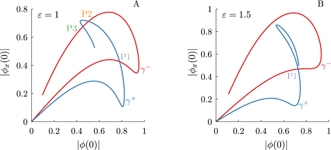
Figure 1: The curves $\gamma^{+}$ (blue) and $\gamma^{-}$ (red) and their intersections (labeled as P1, P2, P3) for $\varepsilon=1$ (panel A) and $\varepsilon=1.5$ (panel B). For all curves, $C^{\pm}\in[0,40]$. Here $\mu=1$.

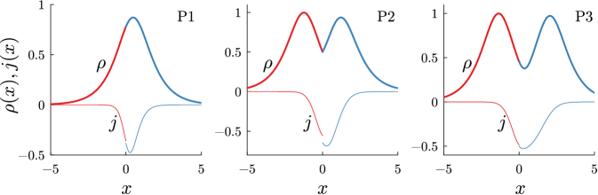
Figure 2: Shapes of the pseudo-modes corresponding to the intersection points P1, P2, P3 in Fig. 1.

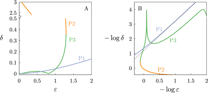
Figure 3: Dependencies of $\delta$ plotted with linear scale (A) and with log-log scale (B). For the reference, in (B) we also plot the straight dotted line with the slope equal to two. In the linear scale, this line corresponds to $\delta\propto\varepsilon^{2}$. Notice that the vertical axis is broken in (A). Labels P1, P2, P3 correspond to the intersection points in Fig. 1. Here $\mu=1$.

As an example, we chose a nonsymmetric W-dW potential of the class (23) having

$$W_{1}(x)=-\frac{1}{e^{x}+e^{-3x}},\quad W_{2}(x)=\frac{e^{x}-3e^{-3x}}{(e^{x}+e^{-3x})^{2}}.$$ (38)

Figure 1 presents two plots of curves $\gamma^{\pm}$ computed for $\mu=1$ and two different values of $\varepsilon$. We observe that the curves can have multiple intersection points, and for different $\varepsilon$ the shapes of the curves can be significantly different, i.e., the intersection points can emerge or disappear as $\varepsilon$ changes. Here we focus on three first intersection points that are labeled as P1, P2, P3 in Fig. 1(A). Notice that with the increase of $\varepsilon$ points P2 and P3 merge and then disappear as illustrated in Fig. 1(B). To visualize the pseudo-modes that correspond to the chosen intersection points, we introduce real-valued piecewise-defined functions

$$\rho(x)=\left\{\begin{array}[]{cc}|\phi^{-}(x)|,&x\leq 0,\\[5.69054pt] |\phi^{+}(x)|,&x\geq 0,\end{array}\right.\quad j(x)=\left\{\begin{array}[]{cc}i(\overline{\phi^{-}_{x}}\phi^{-}-\overline{\phi^{-}}\phi^{-}_{x}),&x\leq 0,\\[5.69054pt] i(\overline{\phi^{+}_{x}}\phi^{+}-\overline{\phi^{+}}\phi^{+}_{x}),&x\geq 0.\end{array}\right.$$

These functions do not depend on the rotation $\theta$ and are therefore especially convenient. Hereafter the overline means complex conjugation. Notice that in the physical context function $j(x)$ can be interpreted as energy flux across the (pseudo)-mode. By construction, for each pseudo-mode $\rho(x)$ is continuous, but it is not necessarily smooth; function $j(x)$ must be continuous for authentic stationary modes, but may have a discontinuity at $x=0$ for pseudo-modes.

Figure 2 presents the pseudo-modes corresponding to intersections P1, P2, and P3. We observe that for each shown pseudo-mode the corresponding function $j(x)$ has a jump at $x=0$. Additionally, for P2 the cusp of $\rho(x)$ is well-visible at $x=0$. The pseudo-mode at the first intersection point P1 resembles the bright soliton, i.e., corresponds to the approximate solution constructed above in Sec. II by means of the asymptotic expansions. Solutions at the next intersections P2 and P3 have more sophisticated shapes and therefore cannot be captured by the asymptotic expansions developed above.

Discontinuous shapes of pseudo-modes plotted in Fig. 2 suggest that those solutions do not correspond to authentic continuously differentiable stationary modes. Indeed, evaluating the solvability indicator $\delta$, we observe that it is generically different from zero. Dependencies $\delta$ on $\varepsilon$ are presented in Fig. 3 in linear and log-log scales. For the simple pseudo-mode corresponding to the first intersection point P1 we observe that the dependence of $\log\delta$ on $\log\varepsilon$ is well approximated by linear function with the slope close to 2. This again agrees with the above asymptotic analysis and suggests that this pseudo-mode solves Eq. (4) for all $x$ except for $x=0$, where the derivative of function $\phi(x)$ has a jump that is of order $O(\varepsilon^{2})$.

For the pseudo-modes corresponding to P2 and P3, the dependencies $\delta(\epsilon)$ are more sophisticated and cannot be described by a simple quadratic law. In the meantime, it is remarkable, that for $\varepsilon\approx 0.8$ the $\delta(\varepsilon)$-function corresponding to P3 has a zero [in the log-log plot in Fig. 3(B) it corresponds to a spike]. This suggests that for some isolated value of $\varepsilon$ close to 0.8 an authentic continuously differentiable solution can potentially be found. Solutions of this type will be discussed below in Sec. V. Summarizing the analysis of the present section, we have to conclude that for an arbitrarily chosen value of $\varepsilon$, Eq. (4) with potential (38) only admits pseudo-modes and no stationary modes.

IV Nonlinear dynamics in W-$\rm d$W potentials

The goal of this section is to elucidate nonlinear dynamics governed by the time-dependent equation (3) with a W-dW potential. One of important analytical results of this section consists in the approximate conservation law that constraints the nonlinear dynamics in W-dW potentials. A dynamical invariant of motion for solitons in W-dW potentials has been earlier reported on in Kominis_OC15 ; Kominis_PRA15 . Our result differs from the previous in two important aspects. First, the dynamical invariant from Kominis_OC15 ; Kominis_PRA15 is obtained with a qualitative approach which treats a soliton as a particle with some mass, velocity and position. However, in the framework of the time-dependent Eq. (3), some of the effective quantities (namely, the soliton position and velocity) are not well-defined. Our conservation law is obtained in terms of the wavefunction $\Phi$. It does not rely on the effective-particle formalism and is therefore valid for localized nonlinear waves of arbitrary shape (not necessarily single-soliton-shaped). Second, our conservation law is only approximate. Our dynamical invariant is exactly time-independent only in the limit of zero amplitude of W-dW potential, while for nonzero $\varepsilon$ the temporal derivative of our invariant is of the $\varepsilon^{2}$-order. In this section we also perform numerical dynamical runs of the time-dependent equation (3) and observe that even though the pseudo-modes do not correspond to authentic stationary states, they feature meaningful nonlinear dynamics associated with the persistent oscillations of the soliton center around the position $x_{0}$ obtained from the above asymptotic analysis.

IV.1 Approximate conservation law and necessary steady-state conditions

A natural question emerges on whether the pseudo-modes encountered in the previous sections have any signature in the nonlinear time-dependent dynamics governed by the non-stationary equation (3). This issue will be addressed in the present section. However, let us first outline some general features of nonlinear dynamics in W-dW potentials. Let $\Phi(x,t)$ be a localized wavepacket whose dynamics is governed by equation (3). We introduce the squared $L^{2}$-norm of the solution (in the optical context it can be interpreted as the beam power) and the location of the center of the wavepacket:

$$N(t)=\int_{-\infty}^{\infty}|\Phi|^{2}dx,\quad X(t)=N^{-1}(t)\int_{-\infty}^{\infty}x|\Phi|^{2}dx.$$ (39)

Computing the temporal derivative of $N(t)$ we obtain the standard “balance equation”

$$N_{t}=2\varepsilon\int_{-\infty}^{\infty}W_{2}|\Phi|^{2}dx.$$ (40)

For a shape-preserving stationary mode $\Phi=e^{i\mu t}\phi(x)$ this gives an obvious condition

$$2\varepsilon\int_{-\infty}^{\infty}W_{2}|\phi|^{2}dx=-\frac{2\varepsilon}{C}\int_{-\infty}^{\infty}W_{1}\left(\frac{d\,}{dx}|\phi|^{2}\right)dx=0.$$ (41)

This condition generalizes that derived above in the first-order perturbation theory [see Eq. (12)].

Additionally, introducing the momentum $P(t)=i\int_{-\infty}^{\infty}(\overline{\Phi_{x}}\Phi-\Phi_{x}\overline{\Phi})dx$, from Eq. (3) we compute

$$P_{t}=-2C\varepsilon\int_{-\infty}^{\infty}W_{2}|\Phi|^{2}dx+2i\varepsilon\int_{-\infty}^{\infty}W_{2}(\Phi_{x}^{*}\Phi-\Phi_{x}\Phi^{*})dx.$$ (42)

An additional calculation yields

$$\varepsilon\frac{d\,}{dt}\int_{-\infty}^{\infty}W_{1}|\Phi|^{2}dx=i\varepsilon C\int_{-\infty}^{\infty}W_{2}(\Phi_{x}^{*}\Phi-\Phi_{x}\Phi^{*})dx+2\varepsilon^{2}\int_{-\infty}^{\infty}W_{1}W_{2}|\Phi|^{2}dx.$$ (43)

Combining the latter relations with (40) and (42), we obtain

$$\frac{d\,}{dt}\left(P+CN-\frac{2\varepsilon}{C}\int_{-\infty}^{\infty}W_{1}|\Phi|^{2}dx\right)=-\frac{4\varepsilon^{2}}{C}\int_{-\infty}^{\infty}W_{1}W_{2}|\Phi|^{2}dx.$$ (44)

For small $\varepsilon$, the latter equality can be considered as an “approximate” conservation law which is specific to small-amplitude W-dW potentials. In the line with findings of Sec. II, this result indicates that a careful attention to the $\varepsilon^{2}$-order-behavior is crucial for the most precise description of nonlinear waves in W-dW potentials.

For a stationary mode, the left-hand side of (44) is zero, which leads to another necessary condition for the shape of the solitary state:

$$-\frac{4\varepsilon^{2}}{C}\int_{-\infty}^{\infty}W_{1}W_{2}|\phi|^{2}dx=\frac{2\varepsilon^{2}}{C^{2}}\int_{-\infty}^{\infty}W_{1}^{2}\left(\frac{d\,}{dx}|\phi|^{2}\right)dx=0.$$ (45)

Introducing the transverse current $j(x)$ across the stationary state

$$j(x)=i(\overline{\phi_{x}}\phi-\overline{\phi}\phi_{x}),$$ (46)

we obtain the standard result which interrelates the derivative of the current and the gain-and-loss distribution:

$$j_{x}=2\varepsilon W_{2}|\phi|^{2}.$$ (47)

More interestingly, for W-dW potentials we obtain

$$C\int_{-\infty}^{\infty}j(x)W_{2}(x)dx+2\varepsilon\int_{-\infty}^{\infty}W_{1}W_{2}|\phi|^{2}dx=0.$$ (48)

Therefore, condition (45) is equivalent to

$$\int_{-\infty}^{\infty}j(x)W_{2}(x)dx=0.$$ (49)

Comparing (41) and (49), we observe that for a stationary mode the imaginary part of the potential $W_{2}$ must be orthogonal not only to the squared modulus of the wavefunction but also to the shape the transverse current distribution.

IV.2 Numerical simulations of nonlinear dynamics

Let us now turn to dynamics of the pseudo-mode solitary waves that satisfy Eq. (4) with $\varepsilon^{2}$-accuracty (see Sec. II). As a model example, we again choose the W-dW potential (23). First, we solve the Cauchy problem with the initial condition $\Phi(x,0)={\operatorname{sech}}(x-x_{0})$, where $x_{0}$ is chosen to satisfy the compatibility condition (12) that emerges in the first order of the perturbation procedure. Numerical solution of Eq. (12) gives $x_{0}\approx 0.4640$. Representative examples of our dynamical simulations are shown in Fig. 4 for the squared norm $N(t)$ and center of mass $X(t)$. For sufficiently small $\varepsilon$ we observe that the plotted characteristics feature small-amplitude nearly periodic oscillations. For small $\varepsilon$ the periodicity is almost perfect, whereas for larger $\varepsilon$ a slow drift appears. Amplitude of the oscillations and the drift velocity naturally become stronger with the increase of amplitude of the potential $\varepsilon$.

Next, we address the situation when the initial condition $\Phi(x,0)={\operatorname{sech}}(x-\tilde{x})$ is situated at a different position than that prescribed by the asymptotic analysis, i.e., $\tilde{x}\neq x_{0}$. The results plotted in Fig. 5 show that for small $\varepsilon$ the center of initially displaced wavepacket performs nearly perfect periodic oscillations around $x_{0}$, and the amplitude of the oscillations increases with the increase of the initial displacement $|\tilde{x}-x_{0}|$. This suggests that even though there is no authentic stationary mode existing at $x=x_{0}$, this asymptotically predicted position still plays an important role in the nonlinear dynamics. For extremely large initial positions $\tilde{x}$, the initial soliton is situated in an effectively homogeneous medium, because the numerical value of the exponentially decaying potential becomes zero for large $x$. In this situation the periodic oscillations naturally disappear.

Representative plots illustrating evolution of the amplitude $|\Phi(x,t)|$ are presented in Fig. 6.

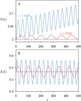
Figure 4: Results of the nonlinear dynamics simulations for $\varepsilon=0.01$ (red color) and $\varepsilon=0.05$ (blue color) for the initial condition $\Phi(x,0)={\operatorname{sech}}(x-x_{0})$, where $x_{0}$ is a solution of (12).

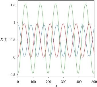
Figure 5: Results of the nonlinear dynamics simulation for $\Phi(x,0)={\operatorname{sech}}(x-\tilde{x})$ when the initial center of the wavepacket $X(0)=\tilde{x}$ is different from the value $x_{0}$ predicted by the asymptotic analysis. Three curves correspond to $\tilde{x}=x_{0}\pm x_{0}$ (blue and red curves, respectively) and to $\tilde{x}=-x_{0}$ (green curve). In all cases $\varepsilon=0.01$. Horizontal dashed line corresponds to $X=x_{0}$.

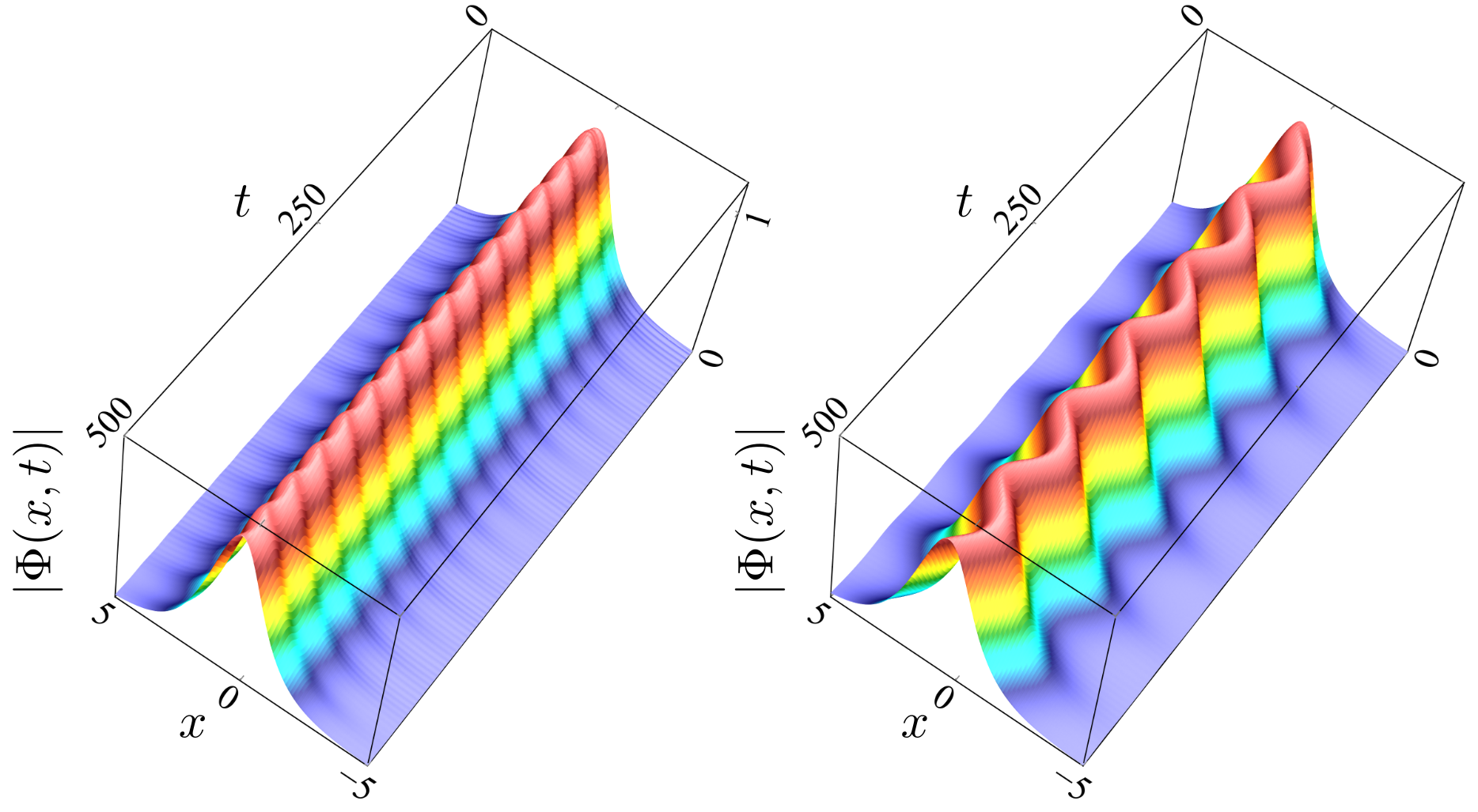
Figure 6: Plot of the amplitude $|\Phi(x,t)|$ for initial condition $\Phi(x,0)={\operatorname{sech}}(x-\tilde{x})$ when $\varepsilon=0.05$ and $\tilde{x}=x_{0}$ (left panel) and $\varepsilon=0.01$ and $\tilde{x}=-x_{0}$ (right panel).

V Nonlinear modes for isolated values of $\varepsilon$

In this section, we we complement our study by numerical computing the authentic stationary modes. They are found using the extension of the numerical shooting approach described above in Sec. III. In contrast to the main outcome of Ref. KCKFB19 , we find that stationary nonlinear modes in a generic W-dW potential of fixed amplitude do not form a continuous family, but exist only at isolated values of the the propagation constant $\mu$. The found authentic nonlinear modes have complex two-hump shapes. Their dynamics is unstable.

As explained above, for a continuously differentiable stationary mode $\phi(x)$ the resulting system of matching conditions (28)-(31) cannot be generically solved if the values of $\varepsilon$ and $\mu$ are fixed. However, if $\varepsilon$ or $\mu$ is treated as another unknown, then the system of four equations is no longer overdetermined, and a numerical solution can be found by Newton iterations. A good initial guess for the iterative procedure is given by the pseudo-mode with $\mu=1$ and $\varepsilon=0.8$ which corresponds to the intersection point P3 (see the corresponding panel in Fig. 2). In Fig. 7 we illustrate a numerically found branch of nonlinear modes in terms of dependencies $\varepsilon(\mu)$ and $N(\mu)$, where $N=\int_{-\infty}^{\infty}|\phi(x)|^{2}dx$. We stress that the shown dependencies do not represent a continuous family, because they can exist only if $\mu$ and $\varepsilon$ are varied simultaneously. For instance, for $\mu=1$, the nonlinear mode can only be found at the isolated value $\varepsilon\approx 0.809$.

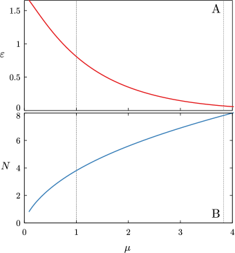
Figure 7: Dependencies $\varepsilon(\mu)$ and $N(\mu)$ for authentic nonlinear modes. Vertical dotted lines correspond to values of $\mu$ for solutions shown in Fig. 8.

Representative shapes of the stationary modes are exemplified in Fig. 8(A,B) in terms of the amplitude $\rho=|\phi|$ and the current $j(x)$. We observe that the amplitude has a distinctively double-hump shape and features a local minimum approximately at the minumum of the real part of the potential. On the other hand, the current $j(x)$ is dominantly negative, which agrees with the spatial distribution of the gain-and-losses [see the imaginary part of the potential plotted in Fig. 8(a)]. The maximal negative value of the current is approached at the local minima of the real part of the potential. For small values of $\varepsilon$, the form of the stationary state resembles a bound state of two elementary nonlinear modes.

The eccentric shape of the obtained nonlinear modes suggests that they can hardly be stable. The instability was indeed confirmed using the linear stability analysis. Following to the standard procedure Yang2010 , we consider a perturbed solution $\Phi(x,t)=e^{i\mu t}[\phi(x)+u(x)e^{i\omega t}+\bar{v}(x)e^{-i\bar{\omega}t}]$, where $u(x)$ and $v(x)$ are small perturbations. Linearization of Eq. (3) with respect to $u(x)$ and $v(x)$ gives the linear stability eigenvalue problem

$$\left(\begin{array}[]{cc}\partial_{x}^{2}-\mu-\varepsilon(W_{1}+iW_{2})+4|\phi|^{2}&2\phi^{2}\\ -2\bar{\phi}^{2}&-\partial_{x}^{2}+\mu+\varepsilon(W_{1}-iW_{2})-4|\phi|^{2}\end{array}\right)\left(\begin{array}[]{c}u\\ v\end{array}\right)=\omega\left(\begin{array}[]{c}u\\ v\end{array}\right).$$ (50)

Unstable modes correspond to eigenvalues $\omega$ with negative imaginary parts.

Numerical solution of the linear stability eigenvalue problem reveals several unstable eigenvalues in the spectrum, see the eigenvalue portraits in Fig. 8(C,D). A closer inspection indicates that, in the contrast with situation that takes place for real-valued potentials, ${\cal PT}$-symmetric potentials ZezKon12 , and Wadati potentials Yang16 , in the case at hand the eigenvalues that emerge in linearization spectra do not form quartets $(\omega,\bar{\omega},-\omega,-\bar{\omega})$. This fact provides another validation of the essentially dissipative nature of W-dW potentials.

Simulating nonlinear dynamics of found stationary modes [exemplified in Fig. 9], we observe that for larger $\varepsilon$ the mode breaks up into two solitary waves that move in opposite directions and eventually leave the domain where the complex potential is localized. In the meanwhile, for smaller $\varepsilon$ only one solitary wave escapes, while the second one performs periodic movement which resembles the oscillations of pseudo-modes observed in Sec. IV.

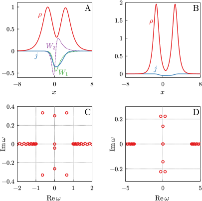
Figure 8: Shapes of stationary modes for $\mu=1$, $\varepsilon\approx 0.091$ (A) and $\mu\approx 3.830$, $\varepsilon\approx 0.068$ (B). Red and blue curves correspond to the modulus $\rho(x)=|\phi(x)|$ and current $j(x)$, respectively. Dashed curves in (A) plot real ($W_{1}$) and imaginary ($W_{2}$) parts of the potential. Lower panels show the linearization eigenvalues.

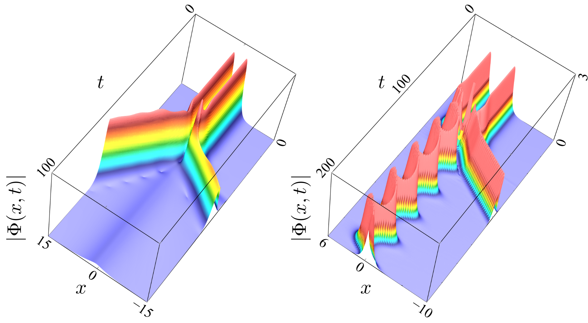
Figure 9: Nonlinear dynamics of stationary modes shown in Fig. 8.

VI Conclusion

In our study, we have examined the peculiar features of a recently discovered class of complex potentials. More specifically, we have considered the class of W-dW potentials which by definition have the form $W(x)=W_{1}(x)+iCW_{1,x}(x)$, where $W_{1}(x)$ is a differentiable real-valued function, and $C$ is a real. It has been suggested KCKFB19 , that the nonlinear Schrödinger equation (NLSE) with a W-dW potential can support continuous families of stationary solitary-wave nonlinear modes. These objects have been in the focus of the present study. Assuming that the potential is small, of $\varepsilon$-order, we have employed asymptotic methods to search for the stationary nonlinear modes, seeking them in the form of formal power series with respect to $\varepsilon$. The asymptotic procedure stops at the terms of the $\varepsilon^{2}$-order, which leads us to a conjecture that no continuous families of nonlinear modes exist in generic W-dW potentials. In order to validate this hypothesis, we have considered a particular example of the W-dW potential whose real part is a finite-depth well. The prediction of the asymptotic approach has been confirmed by numerical arguments, because instead of any authentic nonlinear mode we have been able to find only a pseudo-mode which solves the equation with $O(\varepsilon^{2})$-accuracy. At the same time, with numerical simulations of nonlinear dynamics in W-dW potentials, we have demonstrated that the pseudo-modes can be dynamically robust in small-amplitude W-dW potentials. More specifically, the dynamics of pseudo-modes reveals persistent oscillations of the center-of-mass around the specific position that characterizes the center of the pseudo-mode in the asymptotic expansion. So, even not being authentic stationary nonlinear modes in the mathematical sense, these objects can be regarded as meaningful physical entities. Finally, we have also computed authentic stationary modes which only exist if the parameters of the equation and of the solution itself are tuned precisely. These stationary modes are unstable, and their dynamical instability reveals several distinctive behaviors.

Examples of physically meaningful “pseudo-modes” (or, more generically, “pseudo-solutions”) are not unheard in the previous literature. For instance, a great number of models where “asymptotics beyond all orders” occurs (see Boyd99 for numerous examples) provide physical objects that cannot be described by idealized mathematical models. One of them is the famous example of $\phi^{4}$ breather that is nonexistent in mathematical sense KS87 ; EKNS88 but that may have “decay timescale … longer than the predicted lifetime of the universe” Boyd90 . Another type of pseudo-solutions that is especially well-known in ${\cal PT}$-symmetric potentials corresponds to the so-called ghost states, which can be found from the stationary nonlinear equation with complex-valued propagation constants $\mu$ ghost01 ; ghost02 ; ghost03 . Even though a ghost state is not a true solution of the time-dependent NLSE, several studies report on that if the imaginary part of $\mu$ is small, then it can dynamically persist as a metastable entity, even if the the coexisting authentic nonlinear modes are unstable. We surmise that the pseudomodes reported herein can be probably also interpreted as ghost states after the consideration is extended to allow $\mu$ to be complex-valued.

To conclude, the search of new complex potentials that admit continuous families of nonlinear modes remains a challenging problem for the future studies. Regarding the particular class of W-dW potentials, we believe that an interesting task is related to a more systematic analysis of oscillating patterns encountered in the nonlinear dynamics. A more systematic study of stationary modes in W-dW potentials is also in order. An especially intriguing issue is the search for stable stationary modes which can eventually exist in W-dW potentials of the form different from that considered herein. While only the case of focusing nonlinearity has been considered herein, the behavior of (pseudo)modes can also be addressed under the the defocusing (repulsive) nonlinearity.

Data availability statement

The data that support the findings of this study are available from the corresponding author upon reasonable request.

Appendix A Calculation of the coefficients for the system (21)-(22).

Direct substitution of (15)-(16) into (19)- (20) yields the system (21)-(22) where (for compactness in what follows we write $\int$ instead of $\int_{-\infty}^{\infty}$, bearing in mind that the integration is always over the whole real axis):

$$A_{11} =\int\left(12u_{0}\tilde{u}_{1}-W_{1}\right)u_{0,x}^{2}~{}dx,$$ (51)

$$A_{12} =\int\left(4u_{0}\tilde{v}_{1}+W_{2}\right)u_{0}u_{0,x}~{}dx,$$ (52)

$$A_{21} =\int\left(4u_{0}\tilde{v}_{1}-W_{2}\right)u_{0}u_{0,x}~{}dx,$$ (53)

$$A_{22} =\int\left(4u_{0}\tilde{u}_{1}-W_{1}\right)u_{0}^{2}~{}dx,$$ (54)

$$F_{1} =\int\left(6u_{0}\tilde{u}_{1}^{2}+2u_{0}\tilde{v}_{1}^{2}-W_{1}\tilde{u}_{1}+W_{2}\tilde{v}_{1}\right)u_{0,x}~{}dx,$$

$$F_{2} =\int\left(4u_{0}\tilde{u}_{1}\tilde{v}_{1}-W_{1}\tilde{v}_{1}-W_{2}\tilde{u}_{1}\right)u_{0}~{}dx.$$

Let us simplify these expressions. In the space of rapidly decreasing functions (Schwartz space) define the inner product of $a(x)$ and $b(x)$ as

$$\langle a(x),b(x)\rangle:=\int a(x)b(x)~{}dx.$$

The operators ${\cal L}_{2}$ and ${\cal L}_{6}$ are self-adjoint, therefore

$$\langle{\cal L}_{2}a(x),b(x)\rangle=\langle a(x),{\cal L}_{2}b(x)\rangle,\quad\langle{\cal L}_{6}a(x),b(x)\rangle=\langle a(x),{\cal L}_{6}b(x)\rangle.$$

Also we make use of the fact that by construction [see equations (9)–(10) and (15)–(16)]

$${\cal L}_{6}\tilde{u}_{1}=W_{1}u_{0},\quad{\cal L}_{2}\tilde{v}_{1}=W_{2}u_{0}.$$

1. Consider $A_{12}$.

$$A_{12}=\int\left(4u_{0}\tilde{v}_{1}+W_{2}\right)u_{0}u_{0,x}~{}dx=4\int u_{0}^{2}u_{0,x}\tilde{v}_{1}~{}dx+\langle u_{0,x},{\cal L}_{2}\tilde{v}_{1}\rangle.$$

The last term can be transformed as follows

$$\langle u_{0,x},{\cal L}_{2}\tilde{v}_{1}\rangle=\langle{\cal L}_{2}u_{0,x},\tilde{v}_{1}\rangle=-4\langle u_{0}^{2}u_{0,x},\tilde{v}_{1}\rangle=-4\int u_{0}^{2}u_{0,x}\tilde{v}_{1}~{}dx.$$

Here we make use of the formula ${\cal L}_{6}u_{0,x}=0$ that implies that

$${\cal L}_{2}u_{0,x}=-4u_{0}^{2}u_{0,x}.$$ (55)

Therefore $A_{12}=0$.

2. Consider $A_{22}$.

$$A_{22}= \int(4u_{0}{\tilde{u}}_{1}-W_{1})u_{0}^{2}~{}dx=4\int u_{0}^{3}{\tilde{u}}_{1}~{}dx-\langle{\cal L}_{6}\tilde{u}_{1},u_{0}\rangle$$

$$=4\int u_{0}^{3}{\tilde{u}}_{1}~{}dx-\langle\tilde{u}_{1},{\cal L}_{6}u_{0}\rangle.$$

Since ${\cal L}_{2}u_{0}=0$ then ${\cal L}_{6}u_{0}=4u_{0}^{3}$. Therefore

$$A_{22}=4\int u_{0}^{3}{\tilde{u}}_{1}~{}dx-\langle\tilde{u}_{1},4u_{0}^{3}\rangle=0.$$

3. Consider $A_{21}$.

$$A_{21}=A_{12}-2\int W_{2}u_{0}u_{0,x}dx=-2\langle{\cal L}_{2}\tilde{v}_{1},u_{0,x}\rangle=8\int\tilde{v}_{1}u_{0}^{2}u_{0,x}dx,$$

where we have again used (55).

4. Consider $A_{11}$.

$$A_{11}=12\int u_{0}\tilde{u}_{1}u_{0,x}^{2}dx-\int W_{1}u_{0,x}^{2}dx=12\int u_{0}\tilde{u}_{1}u_{0,x}^{2}dx+\int u_{0}(W_{1,x}u_{0,x}+W_{1}u_{0,xx})dx=$$

$$12\int u_{0}\tilde{u}_{1}u_{0,x}^{2}dx+C\int u_{0,x}W_{2}u_{0}dx+\int W_{1}u_{0}(u_{0}-2u_{0}^{3})dx=$$

$$12\int u_{0}\tilde{u}_{1}u_{0,x}^{2}dx+C\langle{\cal L}_{2}\tilde{v}_{1},u_{0,x}\rangle+\langle{\cal L}_{6}\tilde{u}_{1},u_{0}\rangle-2\langle{\cal L}_{6}\tilde{u}_{1},u_{0}^{3}\rangle=$$

$$12\int u_{0}\tilde{u}_{1}u_{0,x}^{2}dx-4C\int\tilde{v}_{1}u_{0}^{2}u_{0,x}dx+4\int\tilde{u}_{1}u_{0}^{3}dx-2\langle\tilde{u}_{1},{\cal L}_{6}u_{0}^{3}\rangle.$$ (56)

Straightforward computation yields ${\cal L}_{6}u_{0}^{3}=6u_{0}u_{0,x}^{2}+2u_{0}^{3}$. This implies that the first, third and fourth summands in (56) annihilate, and we finally obtain

$$A_{11}=-4C\int\tilde{v}_{1}u_{0}^{2}u_{0,x}dx.$$

5. Consider $F_{2}$.

$$F_{2}=4\int u_{0}^{2}\tilde{u}_{1}\tilde{v}_{1}dx-\int W_{1}u_{0}\tilde{v}_{1}dx-\int W_{2}u_{0}\tilde{u}_{1}dx=4\int u_{0}^{2}\tilde{u}_{1}\tilde{v}_{1}dx-\langle{\cal L}_{6}\tilde{u}_{1},v_{1}\rangle-\int W_{2}u_{0}\tilde{u}_{1}dx=$$

$$=4\int u_{0}^{2}\tilde{u}_{1}\tilde{v}_{1}dx-\int\tilde{u}_{1}(W_{2}u_{0}+4u_{0}^{2}\tilde{v}_{1})dx-\int W_{2}u_{0}\tilde{u}_{1}dx=-2\int W_{2}u_{0}\tilde{u}_{1}dx,$$

where we have used the equality ${\cal L}_{6}\tilde{v}_{1}=W_{2}u_{0}+4u_{0}^{2}\tilde{v}_{1}$ which can be derived easily.

5. Consider $F_{1}$. Since its calculation is a bit more involved, we decompose $F_{1}$ into four summands representing $F_{1}=I_{1}+I_{2}+I_{3}+I_{4}$, where

$$I_{1}=6\int u_{0}\tilde{u}_{1}^{2}u_{0,x}dx,\quad I_{2}=2\int u_{0}\tilde{v}_{1}^{2}u_{0,x}dx,$$

$$I_{3}=-\int W_{1}\tilde{u}_{1}u_{0,x}dx,\quad I_{4}=\int W_{2}\tilde{v}_{1}u_{0,x}dx.$$

The calculation proceeds as follows:

$$I_{3}=\int u_{0}(W_{1,x}\tilde{u}_{1}+W_{1}\tilde{u}_{1,x})dx=C\int u_{0}W_{2}\tilde{u}_{1}+\langle{\cal L}_{6}\tilde{u}_{1},\tilde{u}_{1,x}\rangle.$$ (57)

Straightforward differentiation yields ${\cal L}_{6}\tilde{u}_{1,x}=W_{1,x}u_{0}+W_{1}u_{0,x}-12u_{0}u_{0,x}\tilde{u}_{1}$, which after substitution in (57) eventually leads to

$$I_{3}=2C\int u_{0}W_{2}\tilde{u}_{1}dx-I_{3}-2I_{1},$$ (58)

and hence

$$I_{1}+I_{3}=C\int u_{0}W_{2}\tilde{u}_{1}dx=-\frac{C}{2}F_{2}.$$ (59)

In a similar manner, using that ${\cal L}_{2}\tilde{v}_{1,x}=W_{2,x}u_{0}+W_{2}u_{0,x}-4u_{0}u_{0,x}\tilde{v}_{1}$, we deduce

$$I_{2}+I_{4}=\int\tilde{v}_{1}(2u_{0}u_{0,x}\tilde{v}_{1}+W_{2}u_{0,x})dx=\frac{1}{2}\int\tilde{v}_{1}(-{\cal L}_{2}\tilde{v}_{1,x}+W_{2,x}u_{0}+3W_{2}u_{0,x})dx=$$

$$\frac{1}{2}\left(-\int W_{2}u_{0}\tilde{v}_{1,x}dx+\int\tilde{v}_{1}(W_{2,x}u_{0}+3W_{2}u_{0})dx\right)=\int\tilde{v}_{1}(W_{2,x}u_{0}+2W_{2}u_{0,x})dx.$$

Combining the latter result with (59), we obtain the final expression for $F_{1}$.

References

-
(1)
N. Akhmediev, A. Ankiewicz, Three sources and three component parts of the concept of dissipative solitons. In: Akhmediev, N, Ankiewicz, A, eds. Dissipative Solitons: From Optics to Biology and Medicine, Lecture Notes in Physics 751. Springer-Verlag; 2008. Pp. 1–29.
doi:10.1007/978-3-540-78217-9_1 - (2) N. N. Rosanov, Dissipative optical solitons, J. Opt. Technol. 76 (2009) 187–198.
-
(3)
Y. V. Kartashov, V. V. Konotop, V. A. Vysloukh and D. A. Zezyulin, Guided Modes and Symmetry Breaking
Supported by Localized Gain. In: Malomed B A, ed. Spontaneous symmetry breaking, self-Trapping, and Josephson oscillations Springer Berlin Heidelberg; 2013. Pp. 167–200.
doi:10.1007/10091_2012_4 - (4) B. A. Malomed, Spatial solitons supported by localized gain, JOSA B 31 (2014) 2460–2475.
- (5) Yu. S. Kivshar, G. P. Agrawal, Optical Solitons: From Fibers to Photonic Crystals, Academic Press, 2003.
- (6) L. Pitaevskii and S. Stringari, Bose-Einstein Condensation, Clarendon Press, Oxford, 2003.
- (7) M. Kunze, T. Küpper, V. K. Mezentsev, E. G. Shapiro, S. Turitsyn, Nonlinear solitary waves with Gaussian tails, Physica D 128 (1999) 273–295.
- (8) Yu. S. Kivshar, T. J. Alexander, S. K. Turitsyn, Nonlinear modes of a macroscopic quantum oscillator, Phys. Lett. A 278 (2001) 225–230.
- (9) G. Theocharis, P. G. Kevrekidis, D. J. Frantzeskakis, and P. Schmelcher, Symmetry breaking in symmetric and asymmetric double-well potentials, Phys. Rev. E 74 (2006) 056608.
- (10) G. L. Alfimov, D. A. Zezyulin, Nonlinear modes for the Gross-Pitaevskii equation — a demonstrative computation approach, Nonlinearity 20 (2007) 2075–2092.
- (11) D. E. Pelinovsky, A. A. Sukhorukov, and Yu. S. Kivshar, Bifurcations and stability of gap solitons in periodic potentials, Phys. Rev. E 70 (2004) 036618.
- (12) D. A. Zezyulin, G. L. Alfimov, V. V. Konotop, and V. M. Pérez-García, Stability of excited states of a Bose-Einstein condensate in an anharmonic trap, Phys. Rev. A 78 (2008) 013606.
- (13) J. Yang, Nonlinear Waves in Integrable and Nonintegrable Systems, SIAM, Philadelphia, 2010.
- (14) D. E. Pelinovsky, Localization in Periodic Potentials: From Schrödinger Operators to the Gross-Pitaevskii Equation, Cambridge University Press, New York, 2011.
- (15) Z. H. Musslimani, K. G. Makris, R. El Ganainy, and D. N. Christodoulides, Optical solitons in -periodic potentials, Phys. Rev. Lett. 100 (2008), 030402.
- (16) V. V. Konotop, J. Yang, D. A. Zezyulin, Nonlinear waves in -symmetric systems, Rev. Mod. Phys. 88 (2016) 035002.
- (17) S. V. Suchkov, A. A. Sukhorukov, J. Huang, S. V. Dmitriev, C. Lee, Yu. S. Kivshar, Nonlinear switching and solitons in -symmetric photonic systems, Laser & Photonic Reviews, 10 (2016) 177–213.
- (18) T. Dohnal and P. Siegl, Bifurcation of eigenvalues in nonlinear problems with antilinear symmetry, J. Math. Phys. 57 (2016) 093502.
- (19) T. Dohnal and D. E. Pelinovsky, Bifurcation of nonlinear bound states in the periodic Gross-Pitaevskii equation with -symmetry, Proceedings of the Royal Society of Edinburgh 150 (2020) 171–204.
- (20) M. Wadati, Construction of parity-time symmetric potential through the soliton theory, J. Phys. Soc. Jpn. 77 (2008) 074005.
- (21) E. N. Tsoy, I. M. Allayarov, F. Kh. Abdullaev, Stable localized modes in asymmetric waveguides with gain and loss, Opt. Lett. 39 (2014) 4215.
- (22) V. V. Konotop, D. A. Zezyulin, Families of stationary modes in complex potentials, Opt. Lett. 39 (2014) 5535.
- (23) J. Yang, Analytical construction of soliton families in one- and two-dimensional nonlinear Schrödinger equations with non-parity-time-symmetric complex potentials, Stud. Appl. Math. 147 (2021) 4–31.
- (24) A. Mostafazadeh, Pseudo-Hermiticity versus PT symmetry: The necessary condition for the reality of the spectrum of a non-Hermitian Hamiltonian, J. Math. Phys. 43 (2002) 205.
- (25) S. Nixon and J. Yang, All-real spectra in optical systems with arbitrary gain-and-loss distributions, Phys. Rev. A 93 (2016) 031802(R).
- (26) Y. Kominis, J. Cuevas-Maraver, P. G. Kevrekidis, D. J. Frantzeskakis, A. Bountis, Continuous families of solitary waves in non-symmetric complex potentials: A Melnikov theory approach, Chaos, Solitons & Fractals 118 (2019) 222–233.
- (27) Y. Kominis, Soliton dynamics in symmetric and non-symmetric complex potentials, Opt. Commun. 334 (2015) 265–272.
- (28) Y. Kominis, Dynamic power balance for nonlinear waves in unbalanced gain and loss landscapes, Phys. Rev. A 92 (2015) 063849.
- (29) M. Yamashita, Melnikov vector in higher dimensions, Nonlinear Anal. Theory Methods Appl. 18 (1992) 657-670.
- (30) S. N. Chow and M. Yamashita, Geometry of the Melnikov vector, Nonlinear Equ. Appl. Sci. 185, 79-148 (1992).
- (31) J. Guckenheimer and P. H. Holmes, 1983 Nonlinear Oscillations, Dynamical Systems and Bifurcations of Vector Fields (Berlin: Springer)
- (32) J. Gruendler, The existence of homoclinic orbits and the method of Melnikov for systems in , SIAM J. Math. Anal. 16 (1985) 907–931.
- (33) V. M. Rothos and T. Bountis, Melnikov’s vector and singularity analysis of periodically perturbed 2 D.O.F Hamiltonian systems. 3DHAM95 NATO ASI proceedings. Kluwer CS, editor; 1999.
- (34) A. Gammal, T. Frederico, and L. Tomio, Improved numerical approach for the time-independent Gross-Pitaevskii nonlinear Schrödinger equation, Phys. Rev. E 60 (1999) 2421.
- (35) D. A. Zezyulin, V. V. Konotop, and G. L. Alfimov, Dissipative double-well potential: Nonlinear stationary and pulsating modes, Phys. Rev. E 82 (2010) 056213.
- (36) D. A. Zezyulin, Y. V. Kartashov, and V. V. Konotop, Stability of solitons in -symmetric nonlinear potentials, EPL 96 (2011) 64003.
- (37) D. A. Zezyulin and V. V. Konotop, Nonlinear modes in the harmonic -symmetric potential, Phys. Rev. A 85 (2012) 043840.
- (38) J. Yang and S. Nixon, Stability of soliton families in nonlinear Schrödinger equations with non-parity-time-symmetric complex potentials, Phys. Lett. A 380 (2016) 3803–3809.
- (39) J. P. Boyd, The Devil’s Invention: Asymptotic, Superasymptotic and Hyperasymptotic Series, Acta Applicandae Mathematica 56 (1999) 1–98.
- (40) H. Segur, M. D. Kruskal, Nonexistence of small-amplitude breather solutions in theory, Phys. Rev. Lett. 58 (1987) 747.
- (41) V. M. Eleonsky, N. E. Kulagin, N. S. Novozhilova and V. P. Silin, Spatially self-localized and periodic solutions of wave equations, Selecta Mathematica Sovietica 7 (1988) 1–14.
- (42) J. P. Boyd, A numerical calculation of a weakly non-local solitary wave: the breather, Nonlinearity 3 (1990) 177.
- (43) A. S. Rodrigues, K. Li, V. Achilleos, P. G. Kevrekidis, D. J. Frantzeskakis, and C. M. Bender, PT-symmetric double well potentials revisited: bifurcations, stability and dynamics, Rom. Rep. Phys. (2013) 65, 5–26.
- (44) H. Cartarius, D. Haag, D. Dast, and G. Wunner, Nonlinear Schrödinger equation for a -symmetric delta-function double well, J. Phys. A: Math. Theor. (2012) 45, 444008.
- (45) P. Li, B. A. Malomed, and D. Mihalache, Symmetry-breaking bifurcations and ghost states in the fractional nonlinear Schrödinger equation with a PT-symmetric potential, Opt. Lett. (2021) 46, 3267–3270.