Superharmonic double-well systems with zero-energy ground states: Relevance for diffusive relaxation scenarios

Abstract

Relaxation properties (specifically time-rates) of the Smoluchowski diffusion process on a line, in a confining potential $U(x)\sim x^{m}$, $m=2n\geq 2$, can be spectrally quantified by means of the affiliated Schrödinger semigroup $\exp(-t\hat{H})$, $t\geq 0$. The inferred (dimensionally rescaled) motion generator $\hat{H}=-\Delta+{\cal{V}}(x)$ involves a potential function ${\cal{V}}(x)=ax^{2m-2}-bx^{m-2}$, $a=a(m),b=b(m)>0$, which for $m>2$ has a conspicuous higher degree (superharmonic) double-well form. For each value of $m>2$, $\hat{H}$ has the zero-energy ground state eigenfunction $\rho_{*}^{1/2}(x)$, where $\rho_{*}(x)\sim\exp-[U(x)]$ stands for the Boltzmann equilibrium pdf of the diffusion process. A peculiarity of $\hat{H}$ is that it refers to a family of quasi-exactly solvable Schrödinger-type systems, whose spectral data are either residual or analytically unavailable. As well, no numerically assisted procedures have been developed to this end. Except for the ground state zero eigenvalue and incidental trial-error outcomes, lowest positive energy levels (and energy gaps) of $\hat{H}$ are unknown. To overcome this obstacle, we develop a computer-assisted procedure to recover an approximate spectral solution of $\hat{H}$ for $m>2$. This task is accomplished for the relaxation-relevant low part of the spectrum. By admitting larger values of $m$ (up to $m=104$), we examine the spectral ”closeness” of $\hat{H}$, $m\gg 2$ on $R$ and the Neumann Laplacian $\Delta_{\cal{N}}$ in the interval $[-1,1]$, known to generate the Brownian motion with two-sided reflection.

I Introduction.

In the presence of confining conservative forces, the Smoluchowski (Fokker-Planck) equation, here considered in one dimension, $\partial_{t}\rho=D\Delta\rho-\nabla(b\rho)=L^{*}\rho$, takes over an initial probability density function (pdf) $\rho_{0}(x)$ to an asymptotic stationary ($L^{*}\rho_{*}(x)=0$) pdf of the Boltzmann form $\rho_{*}(x)=(1/Z)\exp[-U(x)/D]$. Here $b(x)=-\nabla U(x)$ and $Z$ is the $L^{1}(R)$-normalization constant, $D$ stands for the diffusion coefficient, which upon suitable rescaling may be set equal $1$ (the value $1/2$ is often employed in the mathematically oriented research). For the record, we mention that $L^{*}$ denotes the Fokker-Planck operator, while $L$ the diffusion generator of the stochastic process, jph ; pavl .

Given a stationary pdf $\rho_{*}(x)$, one can transform the $L^{1}(R)$ Smoluchowski-Fokker-Planck evolution $\exp(tL_{*})$, $t\geq 0$ to the $L^{2}(R)$ Schrödinger semigroup $\exp(-t\hat{H})$, see e.g. jph -jph1 . A classic factorisation risken of $\rho(x,t)=\Psi(x,t)\rho_{*}^{1/2}(x)$ allows to map the Fokker-Planck dynamics into the the generalized (Schrödinger-type) diffusion problem. In the dimensionally rescaled ($D=1$) form we have:

$$\partial_{t}\Psi=\Delta\Psi-{\cal{V}}\Psi=-\hat{H}\Psi.$$ (1)

Accordingly, the relaxation process $\rho(x,t)\to\rho_{*}(x)$ is paralleled by the $L^{2}(R)$ relaxation $\Psi_{0}(x)\to\Psi(x,t)\to\rho_{*}^{1/2}(x)$. We have $\hat{H}\rho_{*}^{1/2}=0$, hence $\rho_{*}^{1/2}$ is a legitimate zero energy bound state of $\hat{H}$. Moreover, the functional form of the induced (Feynman-Kac by provenience, jph ; vilela ; faris ) potential ${\cal{V}}(x)$ readily follows:

$${\cal{V}}(x)={\frac{\Delta\rho_{*}^{1/2}}{\rho_{*}^{1/2}}}=\frac{1}{2}\left(\frac{b^{2}}{2}+\nabla b\right),$$ (2)

We note that $b(x)=\nabla\ln\rho_{*}(x)=-\nabla U(x)$, jph , streit -turbiner1 .

The eigenvalues of $\hat{H}$, up to an inverted sign, are shared by the Fokker-Planck operator $L^{*}=\Delta-\nabla[b(x)\,\cdot]$ and the diffusion generator $L=\Delta+b(x)\nabla$, jph ; pavl . If we have the spectral solution for $\hat{H}$ in hands, in terms of eigenvalues $\lambda$ and $L^{2}(R)$ eigenfunctions $\Psi_{\lambda}(x)$, then the eigenvalues of $L^{*}$ are $-\lambda$, while the corresponding eigenfunctions appear in the form $\phi_{\lambda}(x)=\Psi_{\lambda}(x)\rho_{*}^{1/2}(x)$. The probability density $\rho(x,t)$, that can be expanded into $\phi_{\lambda}(x)$, will relax exponentially with rates determined by gaps in the energy spectrum of $\hat{H}$. This is what we call the spectral relaxation pattern, c.f. jph ; pavl .

Remark: As a side comment let us add that, while reintroducing the (purely numerical, dimensionless) diffusion coefficient $D\neq 1$, i.e. executing $\Delta\to D\Delta$ in Eq. (1), we need to pass to $\rho_{*}\sim\exp(-U/D)$, and $b=D\nabla\ln\rho_{*}$, which gives Eq. (2) the form ${\cal{V}}=D[\Delta\rho_{*}^{1/2}]/\rho_{*}^{1/2}=(1/2)(b^{2}/2D+\nabla b)$. See e.g. jph , subsection A.3, for a comparative discussion of the harmonic attraction, with $D=1/2$ and $D=1$.

For concreteness, let us invoke the commonly employed in the literature higher degree monomial potentials $U(x)=x^{m}/m,x^{m},mx^{m}$. In a compact notation we have:

$$U(x)={\frac{\kappa_{m}}{m}}x^{m}\Longrightarrow{\cal{V}}(x)={\frac{\kappa_{m}}{2}}x^{m-2}\left[{\frac{\kappa_{m}}{2}}x^{m}-(m-1)\right].$$ (3)

The choice of $\kappa_{m}=1$, $m$ or $m^{2}$ reproduces the above listed functional forms of $U(x)$, in conjunction with the corresponding potentials ${\cal{V}}(x)$. This in turn yields another parametrization of the potential:

$${\cal{V}}(x)=ax^{2m-2}-bx^{m-2},$$ (4)

where $a=\kappa_{m}^{2}/4$ and $b=\kappa_{m}(m-1)/2$.

Accordingly, ${\cal{V}}(x)$ has a definite higher order ($m>2$) double-well structure, with two degenerate symmetric minima at which the potential takes negative values. A local maximum of the potential at $x=0$, equals zero.

Let us recall that in the familiar case of the quartic double-well $\alpha x^{4}-\beta x^{2}$, $\alpha,\beta>0$ (which is not in the family (3)), one is vitally interested in the existence of bound states related to negative eigenvalues of $\hat{H}$, see e.g. jph ; turbiner ; turbiner1 . This is not the case, by construction, for our higher order double-well systems, where the zero eigenvalue is the lowest isolated one in the nonnegative spectrum of $\hat{H}$.

The ground state function $\rho_{*}^{1/2}(x)=(1/\sqrt{Z})\exp[U(x)/2]$ of $\hat{H}$, Eqs. (1)-(3), is unimodal with a maximum at an unstable equilibrium point of the potential ${\cal{V}}(x)$ profile. Thus, in the present case, the preferred location of the diffusing (alternatively - quantum) particle is to reside in the vicinity of the unstable extremum of ${\cal{V}}(x)$. That is contrary to physical intuitions underlying the casual understanding of tunnelling phenomena in a quartic double-well quantum system, c.f. Chapter 4.5 in Ref. bas , see also baner .

It is worthwhile to mention that the instability of the local maximum of the potential profile, has been identified as a source of computational problems in the study of spectral properties of the quartic double-well system, for energies close to to the local maximum. These have been partially overcome in Ref. turbiner1 by invoking non-perturbative methods. On the other hand, the quartic double-well system has received an ample coverage in the literature, mostly in connection with the tunneling-induced spectral splitting of eigenvalues, located below the local maximum value and close to this of the local minimum (stable extremum of the potential at the bottom of each well).

For higher-order double-wells of the form (3), (4), with a local maximum at zero, there are no negative eigenvalues of $\hat{H}$ in existence, jph , while the existence of the positive part of the spectrum may be considered to be granted in the superharmonic regime. We note that Eqs. (1)-(4) provide explicit examples of spectral problems, for which neither a standard semiclassical (WKB) analysis, nor instanton calculus (both routinely invoked in the quartic double-well case) can be applied straightforwardly to evaluate non-zero eigenvalues of $\hat{H}$, or lowest energy gaps, turbiner ; turbiner1 .

We are motivated by the strategy of Refs. streit -faris , of reconstructing the (diffusive) dynamics from the eigenstate (and in particular, from the ground state function) of a given self-adjoint Hamiltonian (energy operator). However, in the present paper we follow the reverse logic, with the stochastic process given a priori and the energy operator and its spectral properties remaining to be deduced. See e.g. an introductory discussion in Ref. turbiner . For the uses of eigenfunction expansions in the construction of transition probability densities of the pertinent diffusion process, see risken ; pavl ; jph .

Our departure point is the confining Smoluchowski process with a predefined drift function, specified type of noise (Brownian motion, e.g. the Wiener process) and an asymptotic stationary probability density function (pdf) in existence. In conformity with Eqs. (1) and (2), the zero energy eigenfunction of $\hat{H}$ is directly inferred (take a square root) from the Boltzmann equilibrium pdf $\rho_{*}(x)$ of the Smoluchowski process. The potential ${\cal{V}}$, Eq. (2), derives from the knowledge of $\rho_{*}^{1/2}(x)$ alone.

The problem is that, for monomial attracting potentials $U(x)\sim x^{m}$ (with drifts of the form $b(x)\sim-x^{m-1}$), we do not know strictly positive eigenvalues in the discrete spectrum of the inferred Schrödinger-type operator $\hat{H}$, nor the related eigenfunctions (c.f. for comparison, a discussion of sextic and decatic potentials in Refs. turbiner ; brandon ; maiz ; okopinska ). No reliable numerical procedures have been developed to this end, and even for moderately large values of $m$ (say $m\geq 100$, known methods (including the Mathematica 12 routines) generally fail.

To establish the relaxation properties (like the time rate of an approach to equilibrium) of the Smoluchowski process, we definitely need to have in hands several exact or approximate eigen-data (basically energy gaps), at the bottom of the nonnegative spectrum of $\hat{H}$. This is the essence of the eigenfunction expansion method, risken ; pavl , while employed in the study of asymptotic properties (e.g. the spectral relaxation) of diffusion processes.

The solvability (in the least the partial one) of involved Schrödinger-type spectral problem appears to mandatory to justify the hypothesis that actually the pertinent diffusion process equilibrates according to the spectral relaxation scenario, see also dubkov ; khar ; sokolov and earlier research on related topics risken , kampen -liu .

In below we shall address this spectral problem, by resorting to approximations of the higher order double-well (3) by a properly tuned rectangular double-well, blinder ; lopez ; jelic . We have benefited from Wolfram Mathematica 12 routines of Ref. blinder , which provide reference eigendata (eigenvalues and eigenfunctions shapes of the energy operator $\hat{H}_{well}$), in the low part of the rectangular well spectrum. The steering parameters of the numerical routine have tuning options, which allow to adjust optimal values of the interior barrier width and size, once the overall (sufficiently large, but finite) height of the double-well boundary walls is selected.

We have numerically tested circumstances under which the nonnegative spectrum actually appears in the vicinity of the potential barrier height value. In such case, the corresponding ground state function is predominantly flat and nearly constant (in the least up to the barrier boundaries). This property is shared by our higher order double-well systems (conspicuously with the growth of $m$).

Of special relevance for the approximation procedure is that for $U(x)=mx^{m}$ (for $U(x)=x^{m}$ as well), the local minima of the inferred potential ${\cal{V}}(x)$ reside in the interior of $[-1,1]\subset R$ for all $m=2n>2$, which enables the fitting of ${\cal{V}}(x)$ to the rectangular double well potential contour, up to an additive ”renormalization” of the bottom energy of the rectangular well. The procedure cannot be straightforwardly extended to encompass the case of $U(x)=x^{m}/m$, $m>2$, for which the local minima of ${\cal{V}}(x)$ are exterior to the interval $[-1,1]$, see e.g. jph .

II Monomial potentials and the induced superharmonic double-wells.

II.1 Properties of $U(x)$, $\rho_{*}(x)$ and $\nabla\rho_{*}^{1/2}(x)$ in the large $m$ regime.

It is a folk wisdom, that a sequence of potentials $U_{m}(x)=(x/L)^{m}/m$, $L>0$, $m$ even, for large values of $m$, can be used as an approximation of the infinite well potential of width $2L$ with reflecting boundaries located at $x=\pm L$, c.f. dubkov ; khar ; dybiec ; dybiec0 . Actually, quite often reproduced statement reads: ”the reflecting boundary can be implemented by considering the motion in a bounding potential $\lim_{m\to\infty}U_{m}(x)$”, khar ; dybiec0 ; dybiec ). Things are however not that simple and obvious, see e.g. jph and references linetsky ; bickel ; pilipenko on the reflected Brownian motion in a bounded domain.

For computational simplicity, we prefer to use the dimensionless notation $x/L\rightarrow x$, next skip the lower index $m$, so passing to $U(x)=x^{m}/m$. The ultimate limiting case (e.g. that of the interval with conjectured reflecting boundaries) is to be supported on the interval $[-1,1]$. Potentials of the form $U(x)=\kappa_{m}x^{m}/m$, Eq. (3), with $\kappa_{m}=1,m,m^{2}$, are employed to the same end, khar ; dybiec0 ; dybiec .

We point out that one needs to observe possibly annoying boundary subtleties. Namely, at $x=\pm 1$, we have the following limiting values of $U(\pm 1)$ (point-wise limits, as $m$ grows to $\infty$)

$$U(x)={\frac{\kappa_{m}}{m}}x^{m}\Rightarrow U(\pm 1)=\left\{{\frac{1}{m}},1,m\right\}\rightarrow\{0,1,\infty\}.$$ (5)

On formal grounds, with reference to the open interval $(-1,1)$ and the complement $R\setminus[-1,1]$ of $[-1,1]$, we have the point-wise limit $U(x)\to\infty$, for all $|x|>1$, as $m\to\infty$, while the interior limit equals zero for all $|x|<1$. In addition to the emergent exterior boundary data (instead of the customary local ones for the Neumann Laplacian), we encounter significant differences in the boundary ($x=\pm 1$) properties of $m\to\infty$ limit of $U(x)$.

These in turn have an impact on the limiting properties of $\rho_{*}(x)$ (and of the prospective ground state function $\rho_{*}^{1/2}(x)$ of $\hat{H}$ ). The outcome appears not to be quite innocent as far as the domain of $\hat{H}$ is concerned. Specifically, if the Neumann Laplacian $\Delta_{\cal{N}}$ is to be spectrally approached/approximated in the $m\to\infty$ limit.

We note that, as $m\to\infty$, we arrive at $\rho_{*}(x)=0$ for all $|x|>1$, while $\rho_{*}(x)=1/2$ for all $|x|<1$. However, the pointwise limit $m\to\infty$ of $\rho_{*}(\pm 1)$ reads, respectively (in correspondence with that for $U(x)$, Eq. (5)):

$${\rho_{*}(\pm 1)}_{m\to\infty}=\left\{\frac{1}{2},\frac{1}{2e},0\right\}.$$ (6)

This implies the Dirichlet-type boundary data for $\rho_{*}^{1/2}(x)$ at boundaries $\pm 1$ of the interval $[-1,1]$. In case of $\kappa_{m}=m^{2}$ we deal with a ”canonical” form of Dirichlet boundaries, since $\rho_{*}^{1/2}(x)$ vanishes at $x=\pm 1$.

The behavior of $U(x)$ and $\rho_{*}(x)$ with the growth of $m$, we depict in Fig. 1 for the case of $U(x)=mx^{m}$. The exemplary functional forms of the inferred potential ${\cal{V}}(x)$ are shown in Fig.2. The conspicuous higher order double well structure is clearly seen.

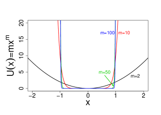
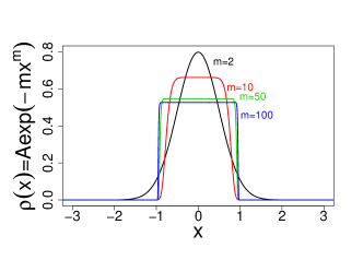
Figure 1: Left panel: $U(x)=mx^{m}$, $m=2n>2$. Right panel: we report exemplary stationary pdfs of the Smoluchowski diffusion process $\rho_{*}(x)=(1/Z)\,\exp[-U(x)]$, $Z=\int_{-\infty}^{+\infty}\exp[-U(x)]dx$. We have $\lim_{m\to\infty}U(x)=\infty$ for all $|x|\geq 1$, and the limiting value $0$ for $|x|<1$. Accordingly, $\rho_{*}(x)\to 0$ for $|x|\geq 1$ and $1/2$ for all $|x|<1$. We note symptoms of the (graphical) convergence towards the constant pdf $1/2$ in $(-1,1)$, which sets an association with the reflected Brownian motion in the interval $[-1,1]$, c.f. jph . One should carefully observe the troublesome point-wise limit (the Dirichlet boundary) of $\rho_{*}(\pm 1)=0$ as $m\to\infty$, see e.g. Eq. (6).

As long as we prefer to deal with traditional Langevin-type methods of analysis, it is of some pragmatic interest to know, how reliable is an approximation of the reflected Brownian motion in $[-1,1]$ by means of the attractive Langevin driving (and thence by solutions of Eq. (1)), with force terms (e.g. drifts) coming from extremally anharmonic (steep) potential wells.

The main obstacle, we encounter here, is that a ”naive” $m=2n\rightarrow\infty$ limit is singular and cannot be safely executed on the level of diffusions proper. We note that for any finite $m$, irrespective of how large $m$ actually is, we deal with a continuous and infinitely differentiable higher order double-well potential and the smooth Boltzmann- type pdf. These properties are broken in the (formal) limit $m\to\infty$.

At this point we recall that for the Neumann Laplacian $\Delta_{\cal{N}}$ on $[-1,1]$, the boundary condition for all its eigenfunctions, bickel ; carlsaw , is imposed locally. In particular, for the ground state function we should have $\Delta_{\cal{N}}\rho_{*}^{1/2}(x)=0$ and $\nabla\rho_{*}^{1/2}(\pm 1)=0$, see e.g. also Ref. carlsaw , chap. 4.1. This formally holds true or a constant function $1/\sqrt{2}$, defined on $[-1,1]$, but can not be achieved through a controlled limiting procedure: $m\to\infty$ of $\nabla\rho_{*}(\pm 1)$.

Indeed, we know from Ref. jph that for $U(x)=x^{m}/2$, the inferred square root of the Boltzmann-type pdf $\rho_{*}^{1/2}(x)=(1/\sqrt{Z})\exp(-x^{m}/2m)$ does not reproduce the Neumann condition in the $m\to\infty$ limit. Namely, we have: $\lim_{m\to\infty}\nabla\rho_{*}^{1/2}(+1)=-1/2\sqrt{2}$.

Since, in accordance with the notation (3) we have:

$$\nabla\rho_{*}^{1/2}(x)=-{\frac{1}{2}}[\nabla U(x)]\rho_{*}^{1/2}(x)$$ (7)

where $\nabla U(x)=\kappa_{m}x^{m-1}$, we can readily complement formulas (5) and (6), by these referring to the limiting behavior of $\nabla\rho_{*}^{1/2}(\pm 1)$:

$${\nabla\rho_{*}^{1/2}(\pm 1)}_{m\to\infty}=\left\{\mp{\frac{1}{2\sqrt{2}}},\mp\infty,\mp\infty\right\}.$$ (8)

Clearly, the point-wise $m\to\infty$ limit of $\nabla\rho_{*}^{1/2}(\pm 1)$ has nothing to do with the Neumann boundary condition, which is not reproduced in this limiting regime. Conseqeuntly, $\rho_{*}^{1/2}(x)$ is not in the domain of the Neumann Laplacian $\Delta_{\cal{N}}$, in plain contradiction with popular expectations, dubkov - dybiec0 .

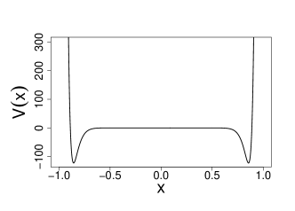
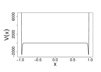
Figure 2: $U(x)=mx^{m}$: the inferred potential ${\cal{V}}(x)={\frac{m^{2}}{2}}x^{m-2}[{\frac{m^{2}}{2}}x^{m}+(1-m)]$ is depicted for $m=20$ and $100$. Note significant scale differences along the vertical axis. Minima of the semigroup potential are located in the interior of $[-1,1]$ for all $m$, and with the growth of $m$, approach $\pm 1$. In parallel, the depth of narrowing local wells escapes to minus infinity, while the ${\cal{V}}(x)=0$ ”plateau” extends to $(-1,1)$. We note that for all $|x|\geq 1$ we have ${\cal{V}}(x)\rightarrow+\infty$.

II.2 Location of the minima $|x_{min}|$ of ${\cal{V}}(x)$ and the large $m$ asymptotics.

We can readily infer the location of (negative) minima of the potential ${\cal{V}}(x)$, c.f. Eq. (3) and Fig. 2, where

$$\mathcal{V}^{\prime}(x)=0\Longrightarrow|x_{min}|=\left[{\frac{b}{2a}}{\frac{m-2}{m-1}}\right]^{1/m}=\left[{\frac{m-2}{\kappa_{m}}}\right]^{1/m}.$$ (9)

For $\kappa_{m}=1$ we have $|x_{min}|=(m-2)^{1/m}>1$ for all $m>2$. For $\kappa_{m}=m$ we obtain $|x_{min}|=[(m-2)/m]^{1/m}<1$, and likewise for $\kappa_{m}=m^{2}$, when $|x_{min}|=[(m-2)/m^{2}]^{1/m}<1$.

We point out that $m^{1/m}>1$ and $\lim_{m\rightarrow\infty}m^{1/m}=1$, c.f. kuczma ; jph . Accordingly, in the large m limit, the minimum locations approach the interval $[-1,1]$ endpoints $\pm 1$, respectively from the interval exterior $R\setminus[-1,1]$ for $\kappa_{m}=1$, or interior of $[-1,1]\subset R$ if otherwise. This behavior is (continuously) depicted in Fig.3.

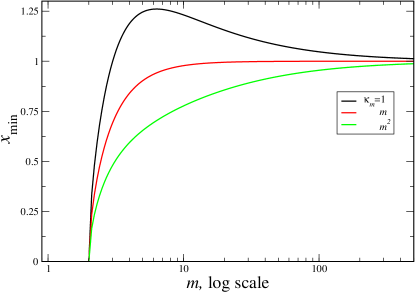
Figure 3: Dependence of $|x_{min}|$ on $m$ (here visualised continuously), for different choices of $\kappa_{m}=\{1,m,m^{2}\}$.

Since we are interested in the large m regime it is useful to rewrite the formula (9) as follows:

$$|x_{min}|=\exp\left\{{\frac{1}{m}}\left[\ln{\frac{m}{\kappa_{m}}}+\ln(1-{\frac{2}{m}})\right]\right\}\sim 1+\frac{\ln(m/\kappa_{m})}{m}-\frac{2}{m^{2}}+\frac{\ln^{2}(m/\kappa_{m})}{2m^{2}},$$ (10)

where $\ln(m/\kappa_{m})=\{\ln m,0,-\ln m\}$, and we have employed the series expansion $\ln(1-x)=-\sum_{n=1}^{\infty}x^{n}/n$, valid in the range $-1\leq x<1$, and here considered for $x=2/m$. In the large $m$ approximate formula (10), expansion terms up to the $m^{-2}$ order have been kept. We recall that $\kappa_{m}=\{1,m,m^{2}\}$.

We immediately realize that in the regime of large $m$, for $\kappa_{m}=1$ the dominant contribution to $|x_{min}|$, Eq. (10), comes from $1+{\frac{\ln m}{m}}$, for $\kappa_{m}=m$ from $1-1/m^{2}$, and for $\kappa_{m}=m^{2}$ from $1-{\frac{\ln m}{m}}$.

Let us denote

$$\triangle=\triangle(m)=|1-|x_{min}||$$ (11)

the distance of $|x_{\min}|$ from the nearby boundary point $\pm 1$. In passing we note that $\triangle\sim\{+{\frac{\ln m}{m}},1/m^{2},{\frac{\ln m}{m}}\}$ for $\kappa_{m}=\{1,m,m^{2}\}$ respectively.

In Fig. 4 we visualize the $m$-dependence of the signed deviation $\delta=1-x_{min}$ of $+1$ from the nearby $x_{min}>0$. For large $m$, we have $\delta\sim\{-{\frac{\ln m}{m}},1/m^{2},{\frac{\ln m}{m}}\}$. For $x_{min}>1$ the signed deviation is negative, and positive for $x_{min}<1$. Note that $\triangle=|\delta|$.

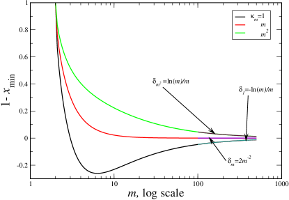
Figure 4: Dependence of $\delta=1-x_{min}$ on $m$, with $x_{min}>0$, while visualised continuously for different choices of $\kappa_{m}=\{1,m,m^{2}\}$.

II.3 Variability of ${\cal{V}}(x)$ in the vicinity of $x=\pm 1$.

By turning back to Eq. (3), plugging there the minimum location value $|x_{min}|$, Eq. (9), we arrive at the following expression for the depth of local wells of the potential (3):

$${\cal{V}}(|x_{min}|)=-{\frac{m\kappa_{m}}{4}}|x_{min}|^{m-2}=-{\frac{m(m-2)}{4}}|x_{min}|^{-2}.$$ (12)

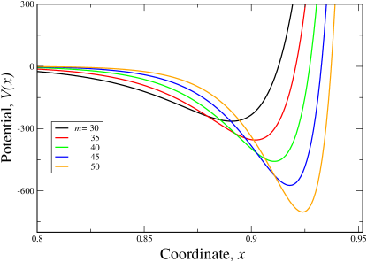
Figure 5: A complement to Fig. 2, with ${\cal{V}}(x)$ inferred from $U(x)=mx^{m}$. Sequential image of local well minima in the vicinity of $x=1$, for moderate values of $m=30,35,40,45,,50$. A flat part of the potential curve ${\cal{V}}(x)\simeq 0$ extends (collectively) between rough values $-0.8$ and $+0.8$. Note that for $m=50$, we have $|x_{min}|\simeq 0,92$, $2\triangle\simeq 0,16$ and the flat part of the potential curve is roughly limited to $[-0,84,+0,84]$.

For sufficiently large values of $m$ (basically above $m=100$), we can pass to rough approximations

$${\cal{V}}(|x_{min}|)\sim-{\frac{m(m-2)}{4}}\sim-{\frac{m^{2}}{4}}.$$ (13)

(We note that in this approximation regime, the well depth becomes independent of the choice of $\kappa_{m}$.) This rough estimate of ${\cal{V}}(|x_{min}|)$, comes from presuming that $|x_{min}|^{-2}\to 1$.

It is instructive to have more detailed insight into the pertinent large $m$ asymptotics. We proceed by repeating basic steps in the derivation of Eq. (10):

$$|x_{min}|^{-2}=\exp\left\{-{\frac{2}{m}}\left[\ln{\frac{m}{\kappa_{m}}}+\ln(1-{\frac{2}{m}})\right]\right\}\sim 1-\frac{2\ln(m/\kappa_{m})}{m}+\frac{4}{m^{2}}+\frac{2\ln^{2}(m/\kappa_{m})}{2m^{2}}.$$ (14)

For large $m$, the dominant contributions read: for $\kappa=1$ we have $1-2{\frac{\ln m}{m}}$, for $\kappa_{m}=m$ we get $1+2/m^{2}$, and for $\kappa_{m}=m^{2}$ we have $1+2{\frac{\ln m}{m}}$. This outcome lends support to our approximation (13) of the well depth.

We recall that for sufficiently large values of $m$, local minimum locations $x_{min}$ are close to $\pm 1$, and in the interval of the size $2\vartriangle$ in the vicinity of $\pm 1$, we encounter rapid (albeit smooth, e.g. continuous and continuously differentiable) variations of ${\cal{V}}(x)$. Considering $m$ to be large, we exemplify this behavior for $\kappa_{m}=m^{2}$, within the interval $1-2\triangle<x_{min}<1$ of length $2\triangle$:

$${\cal{V}}(x_{min}-\triangle)\simeq 0\Rightarrow{\cal{V}}(x_{min})\simeq-{\frac{m(m-2)}{4}}\Rightarrow{\cal{V}}(x_{min}+\triangle)={\cal{V}}(1)={\frac{m^{2}}{2}}\left[{\frac{m^{2}}{2}}-(m-1)\right]\simeq{\frac{m^{4}-2m^{3}}{4}},$$ (15)

We have thus a ”wild” variation of ${\cal{V}}(x)$, ranging from nearly $0$, through (roughly) $-(m^{2}-2m)/4$, to (roughly as well) $+(m^{4}-2m^{3})/4$, in the interval of length $2\triangle\sim 2/m^{2}$.

III Rectangular double-well approximation of the superharmonic double well potential ${\cal{V}}(x)$.

III.1 The fitting procedure.

For further discussion we restrict consideration to the choice of $U(x)=mx^{m}$, with all ensuing formal consequences. Essentially, we need $|x_{min}|<1$ for all $m$, an the point-wise limit of $\lim_{m\to\infty}U(\pm 1)=\infty$. Since $\rho_{*}^{1/2}(\pm 1)_{m\to\infty}=0$, we are tempted to explore an approximation of our higher degree double-well potential function, by means of a sequence of rectangular double well systems, with adjustable (internal) barrier heights and widths, bas .

We anticipate the existence of an affinity between ${\cal{V}}(x)$, as $m$ grows to $\infty$, and a properly tuned rectangular double-well potential, cf. Refs. bas ; blinder ; lopez ; jelic . That is supported by an experimentation with the dedicated Mathematica 12 routine, blinder , created to address the rectangular double-well spectral problem. Fine tuning options concerning the overall depth (large) of the well and the middle barrier size parameters (width and height) allow for a controlled manipulation. Its explicit outcome were lowest eigenvalues and eigenfunctions (up to eight) of the corresponding energy operator $\hat{H}_{well}$, see e.g. blinder .

Numerical tests confirmed that the ground state eigenvalue, which is equal (or in the least nearly equal) to the height of the barrier, is in existence if the proper width/height balance is set. The corresponding ground state eigenfunction is ”flat” (practically constant) in the area of the barrier plateau (local maximum area). This sets a background for a subsequent discussion.

We depart from the ”canonical” qualitative picture of the ammonia molecule, as visualized in terms of the rectangular double well, bas , chap. 4.5. We adopt the original notation of Ref. bas to the graphical description given below, in Figs 6 and 7, see also blinder . One must keep in mind different (D=1 versus D=1/2) scalings of the Laplacian in the employed versions of the rectangular well energy operator.

From the start, we implement the energy scale ”renormalization” of the rectangular double-well energy operator. The original non-negative potential bas ; blinder ; lopez ; jelic is shifted down along the energy axis, by the value of its local maximum (barrier height), from the original minimum value $0$ (well bottom) of the rectangular potential. This in turn enables and effective fitting of the higher order double-well potential to the rectangular double-well potential contour.

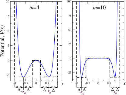
Figure 6: Exemplary fitting of $m=4$ and $m=10$ potentials ${\cal{V}}(x)$ to suitable rectangular double wells. We point out the overall shift of the original rectangular double-well along the energy axis. This assigns the value $0$ to the local maximum (top of the interior barrier) and makes the height of the barrier to quantify the well depth. Here, the interval in use is $[-1,1]$, $\triangle$ stands for a distance between the nearby endpoint $\pm 1$ and the location $\pm x_{0}=x_{min}$ of the local minimum of ${\cal{V}}(x)$. Here $2-2\triangle$ is a provisional measure of the ”plateau” width, of the (fitted) rectangular well barrier.

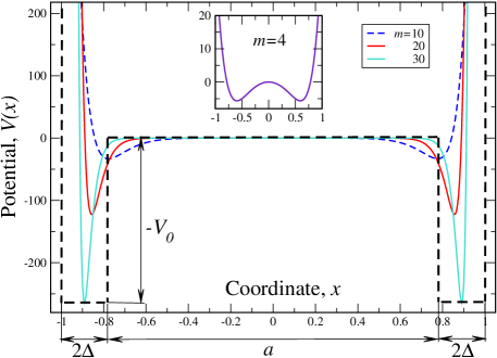
Figure 7: A comparative display of $m=10,20,30$ potentials ${\cal{V}}(x)$, where $x_{0}$, $2\Delta$ and the height $V_{0}$ of the barrier ($-V_{0}$ refers to the depth of the well), actually provide a fit for $m=30$. The $m=4$ potential contour is depicted in the inset.

The fitting procedure, graphically outlined in Figs. 6 and 7, looks promising but is somewhat deceptive. To justify its usefulness, we must first check under what circumstances the rectangular well spectral problem does admit the bottom (ground state) eigenvalue zero. In contrast to the higher order double-well $\hat{H}$, Eqs. (1) to (3), where the zero energy ground state is introduced as a matter of principle, its existence is obviously not the generic property in the rectangular double-well setting. Accordingly, the proposed approximation methodology might seem bound to fail.

Fortunately, we can demonstrate that potentially disparate two-well settings (higher order versus rectangular one), actually coalesce if we look comparatively at the higher $m$ data (say $m\geq 80$) and set them in correspondence with these belonging to the rectangular well system. To this end, let us employ the rectangular double-well lore of Ref. blinder . Temporarily, the notation will at some points differ from this adopted by us in Section III.A.

Following Ref. blinder , we consider the potential $V_{rect}(x)=V(x)=\infty$ for $x<0$ and $x>\pi$, while we assign a constant positive value $V(x)=V_{0}$ for $(\pi-a)/2\leq x\leq(\pi+a)/2$, where $0<a<\pi$, and demand $V(x)=0$ elswhere. This defines a rectangular double well profile immersed in the infinite well. The double well is set on the interval $[0,\pi]$, its bottom is located at the energy value zero, while the barrier with height $V_{0}$ has the width $a$, and separates two symmetrical wells extending over the intervals $[0,(\pi-a)/2]$ and $[(\pi+a)/2,\pi]$.

III.2 The eigenvalue zero in the rectangular double-well setting.

As far as the ground state function and the bottom eigenvalue of $\hat{H}_{rect}=-{\frac{1}{2}}\Delta+V(x)$ is concerned, we have in hands two steering parameters $a$ and $V_{0}$, which can be fine-tuned. In passing, we notice the presence of the $1/2$ factor preceding the Laplacian, and recall that the interval of interest is $[0,\pi]$ instead of $[-1,1]$. This needs to be accounted for, when we shall pass to the spectral comparisons between $\hat{H}_{rect}$ and $\hat{H}$ of Eqs. (1)-(3).

In view of the standard infinite well enclosure, all (piece-wise connected) eigenfunctions are presumed to obey the Dirichlet boundary data: $\psi(0)=0=\psi(\pi)$. We are interested in the ground state function, hence our focus is on even eigensolutions $\psi(x)=\psi(\pi-x)$ of $\hat{H}_{rect}\psi=E\psi$.

In the two local well areas we have $V_{0}(x)=0$ , hence respective even solutions have the self-defining form, blinder ; bas :

$$\psi_{L}(x)=\alpha\sin(kx),\,\,\,0\leq x\leq(\pi-a)/2$$ (16)

and

$$\psi_{R}(x)=\alpha\sin[k(x-\pi)],\,\,\,(\pi-a)/2\leq x\leq\pi$$ (17)

where subscripts $L$ and $R$ refer to the left or right well, respectively. Within the wells we have:

$$-{\frac{1}{2}}{\frac{\Delta\psi(x)}{\psi(x)}}={\frac{k^{2}}{2}}=E.$$ (18)

On the other hand, within the barrier region, the proper form of the even eigenfunction is:

$$\psi_{barrier}(x)=\beta\cosh[{\cal{K}}(x-\pi/2)],\,\,\,(\pi-a)/2\leq x\leq(\pi+a)/2.$$ (19)

Since the total energy is preserved throughout the well and equal $E$, Eq. (18), along the barrier we have:

$$\left[-{\frac{1}{2}}\Delta+V(x)\right]\psi(x)=\left[{\frac{{\cal{K}}^{2}}{2}}+V_{0}\right]\psi(x)=E\psi(x).$$ (20)

Accordingly, for $E\geq V_{0}$, we have

$${\cal{K}}=\sqrt{2V_{0}-k^{2}}=\sqrt{2(V_{0}-E)}.$$ (21)

The connection formulas at the barrier boundaries, may be conveniently expressed as continuity conditions for logartithmic derivatives. For example at $x=(\pi-a)/2$ we require:

$$\nabla\ln\psi_{well}([\pi\mp a]/2)=\nabla\ln\psi_{barrier}([\pi\mp a]/2),$$ (22)

which results in the transcendental equations (for even states):

$$k\cot[k(\pi-a)/2]=-\sqrt{2V_{0}-k^{2}}\tanh[(a/2)\sqrt{2V_{0}-k^{2}}].$$ (23)

We point out, that the regime of $V_{0}\leq E$ may be achieved a formal substitution ${\cal{K}}\rightarrow i{\cal{K}}$, where $i$ is an imaginary unit. This would transform $\cosh({\cal{K}}(x-\pi/2)$ into $\cos({\cal{K}}(x-\pi/2)$, in parallel with the replacement of $V_{0}-E\geq 0$ by $E-V_{0}\geq 0$ in Eq. (21).

The transition point between two spectral regimes $E\leq V_{0}$ and $V_{0}\leq E$ follows from the demand:

$$2V_{0}-k^{2}=0\Longrightarrow k\cot[k(\pi-a)/2]=0$$ (24)

which implies $k=\sqrt{2V_{0}}$ and $E=k^{2}/2=V_{0}$.

The condition (24) sets a relationship between $a$ and $V_{0}$, showing for which pairs ${a,V_{0}}$, the spectral (non-negative) ground state eigenvalue $E=V_{0}$ is admissible. We have:

$$a=a(V_{0})=\pi\left(1-{\frac{1}{\sqrt{2V_{0}}}}\right)$$ (25)

or, equivalently:

$$V_{0}=V_{0}(a)={\frac{\pi^{2}}{2(\pi-a)^{2}}}$$ (26)

which we depict in Fig. 8.

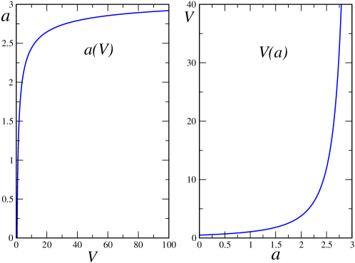
Figure 8: In the left panel we depict a dependence of $a$ upon $V_{0}$, Eq. (25), while meeting the condition (24). In the right panel, we depict the dependence of $V_{0}$ upon $a$, according to Eq. (26).

We note that the condition (22) requires ${\cal{K}}=0$, and in agreement with Eq. (19) identifies $\psi_{barrier}(x)=\beta$ to be constant along the barrier ”plateau”. Given $a$, we have in hands the corresponding barrier height $V_{0}=V_{0}(a)$, Eq. (26). Since $k=\sqrt{2V_{0}}$, we have also in hands an explicit functional form for the left and right well eigenfunction ”tails” $\psi_{L}(x)$ and $\psi_{R}(x)$, c.f. Eqs. (16), (17). We point out the validity of the Dirichlet boundary conditions at $0$ and $\pi$. Moreover, the continuity conditions (22) for logarithmic derivatives at the barrier endpoints, do not need nor necessarily imply the Neumann condition (e.g. the vanishing of derivatives at these points).

Coming back to the comparative (higher order well versus rectangular well) ”eigenvalue zero” issue, let us notice that plugging ${\cal{K}}=0$ in Eq. (20), we need to ”renormalize” the energy scale by subtracting $V_{0}$:

$$\left\{-{\frac{1}{2}}\Delta+[V(x)-V_{0}]\right\}\psi(x)=0.$$ (27)

to pass to the ”eigen-energy zero” regime of the rectangular well problem. This is properly reflected in Figs. 6 to 8. We note, that to maintain the link with the potential (3) for all $m$, we need to allow $V_{0}$ to escape to $\infty$, with $m\to\infty$. This may be considered as a motivaton for invoking the phrase ”additive energy renormalization”, in connection with the $V_{0}$ - subtraction in Eq. (27).

Remark: Let us mention that the zero energy association with the unstable equilibrium of the potential profile, has been discussed for standard quartic double well. A transition value of the well steering parameter has been identified, turbiner ; turbiner1 ; jph , as a sharp divide point between two spectral regimes: nonnegative and that comprising a finite number of negative eigenvalues (near the local minima standard WKB methods give reliable spectral outcomes for the ”normal” double-well system, blinder ; lopez ; jelic ).

IV Discussion of spectral affinites: Superharmonic double well versus rectangular double well.

IV.1 Notational adjustments.

Since some of the defining parameters in the rectangular double-well and in the higher order (superharmonic) double-well differ, we need to analyze means of the removal of this obstacle in our subsequent analysis.

First we shall comparatively address the width/height balance of the barrier in the rectangular case, with its analog (approximate width and the elevation of the ”plateau” above the potential minima, c.f. Fig. 7) in the higher order case. To this end, we need to resolve the $[0,\pi]$ of Fig. 8, versus $[-1,1]$ of Figs. 6 and 7, interval size discrepancy.

We note that it is $U(x)=(x/L)^{m}$, which in the large $m$ regime gives rise to the well with the support on the interval $[-L,L]$ of length $2L$. Setting $L=1$ we recover $[-1,1]$, while $L=\pi/2$ gives rise to $[-\pi/2,\pi/2]$.

These support intervals are examples of centered boxes with the center location $x_{c}=0$. An arbitrarily relocated (shifted) box of length $2L$, if centered around any $x_{c}\in R$ has a support $[x_{c}-L,x_{c}+L]$. Hence, choosing $x_{c}=L$, we pass to the supporting interval $[0,2L]$, which upon the adjustment $L=1\rightarrow L=\pi/2$ leads to the required $[0,\pi]$.

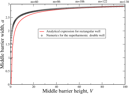
Figure 9: After adjustments of the interval location and length ($[-1,1]\rightarrow[0,\pi]$) and steering parameters $V_{0}$, $a$ (see the text) we have identified when the eigenvalue zero regime of the rectangular double-well actually coalesces with that of the higher order (superharmonic) double-well. A fapp (for all practical purposes) coalescence can be (with quite reasonable accuracy) accepted for $m\geq 84$.

The rectangular well width-height/depth, $a$-$V_{0}$ balance, as depicted in Figs. 7 and 8, is to be compared with the corresponding data of the superharmonic double-well system (1)-(3). To this end, we must recompute the potential (3) minima (their bottom is set at $-V_{0}$ in Figs. 6 to 8), identify the location of $x_{0}$, and next evaluate $4\triangle$, to get the width identifier $a=\pi-4\triangle$. The computation must be accomplished by rescaling everywhere the variable $x$ to the form $x/L$, where $L=\pi/2$. The outcome is presented in the comparative Fig. 9.

To analyze spectral affinities between ${\hat{H}}$ of Eqs. (10-(3) and the rectangular double well Hamiltonian (c.f. Eq. (27)), additional precautions need to be observed. The original numerical evaluation of up to eight eigenvalues and eigenfunctions involves what we have identified as $\hat{H}_{rect}=-{\frac{1}{2}}\Delta+V(x)$, with the detailed definition of the rectangular double-well potential given in Section III.B.

To compare these results with the $[-1,1]$, $D=1$ setting of $\hat{H}$, as visualized in Figs. (6) and (7), all numerically obtained data (we have employed Mathematica 12 routines, blinder ) must ultimately be converted from the original $[0,\pi]$, $D=1/2$ framework to the superharmonic one.

We show how our procedure works, by means of the exemplary data set in Table I. We emphasize that the spectral solution is sought for $\hat{H}_{well}$, and from the outset we are interested in the nonnegative spectrum, including the bottom eigenvalue $E=V_{0}$, or a close neraby candidate value (this computation is quite sensitive to a proper choice of $a$ and $V_{0}$, and basically much more than first four decimal digits are needed to get the exact result (this is untenable within Mathematica routines, hence some flexibility must be admitted).

Once a spectral solution of $\hat{H}_{rect}$ is numerically retrieved, we must compensate the extra factor $D=1/2$ preceding the Laplacian, by considering $2\hat{H}_{rect}$. This amounts to the doubling of all computed eigenvalues.

To enable a comparison with the superharmonic case, we need one more correction, actually a conversion of obtained spectral data to the $[-1,1]$ regime. This may be accomplished by means of a factor $\pi^{2}/4$. In view of the energy doubling, mentioned before, an overall conversion factor reads $2\times(\pi^{2}/4)=\pi^{2}/2$.

numerics, blinder	renormalization	conversion	relabeling
$E_{1}=41,8=V_{0}$	$E_{1}-V_{0}=0$	$\times\pi^{2}/2=0$	$\rightarrow$ $E_{0}$
$E_{2}=42,4$	$E_{2}-V_{0}=0,6$	$2,96$	$\rightarrow E_{1}$
$E_{3}=44,10$	$E_{3}-V_{0}=2,3$	$11.35$	$\rightarrow E_{2}$
$E_{4}=46,9$	$E_{4}-V_{0}=5,1$	$25,167$	$\rightarrow E_{3}$
$E_{5}=50,8$	$E_{5}-V_{0}=9,0$	$44,41$	$\rightarrow E_{4}$
$E_{6}=55,8$	$E_{6}-V_{0}=14,0$	$69,087$	$\rightarrow E_{5}$

Table 1: Exemplary data conversion table for Mathematica 12 spectral outcomes of the rectangular double well, blinder . Input data: overall well width $[0,\pi]$, height of the barrier $V_{0}=41,8$, barrier width $a=2,96$, the multiplicative conversion factor for the spectrum is $\pi^{2}/2=4,9348$. Output data: overall well width $[-1,1]$, depth of each well is $-V_{0}$, the ”plateau” $V(x)=0$ width contraction factor is $2/\pi$ (takes $L=\pi$ into $L=2$). Hence the ”plateau” size is $2,96\times(2/\pi)=1,8754$.

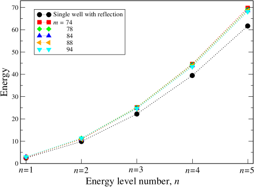
Figure 10: We depict comparatively positive eigenvalues of the ”renormalized” operator $\hat{H}_{ren}$, Eq. (28), on [-1,1], while set in correspondence with the superharmonic $\hat{H}$ for $\kappa_{m}=m^{2}$, and these corresponding to the standard Neumann spectral problem on $[-1,1]$ (here named ”single well with reflection”). In addition to graphical comparisons, in Table II we collect numerically and analytically computed eigenvalues, in their explicit form.

In below, in Table II we reproduce five lowest positive eigenvalues $E_{n}(m),i=1,2,3,4,5$ of the ”renormalized” rectangular double well energy operators

$$\hat{H}_{ren}=-\Delta+2[V(x)-V_{0}],$$ (28)

while set on [-1,1], provided $V(x)$ is the best approximate fit to $m=74,78,84,88,94$ superharmonic potential ${\cal{V}}(x)$, $\kappa_{m}=m^{2}$. These numerical outcomes are set in comparison with positive eigenvalues of the Neumann operator $-\Delta_{\cal{N}}$ on $[-1,1]$, $E_{n}=(\pi^{2}/4)n^{2}$.

We point out that $E_{n}(m)$ outcomes of Mathematica 12 routines, blinder , for the rectangular double-well, Table II, originally refer to the interval $[0,\pi]$, the diffusion coefficient $D=1/2$ and the barrier height $V_{0}(m)$. The reproduced data follow from the $(\pi^{2}/2)[E_{n}(m)-V_{0}(m)]$ conversion recipe, where the data-converting coefficient $\pi^{2}/2$ adjusts the original rectangular well data to the $[-1,1]$, $D=1$ setting. See e.g. a complementary Fig. 11.

$n$	1	2	3	4	5
well	2.4674	9.8696	22.2066	39.4784	61.6850
$m=74$	2.6647	11.054	25.16785	44.6106	69.78
$m=78$	2.961	11.35	25.1675	44.4132	69.1
$m=84$	2.961	10.86	24.674	43.92	68.594
$m=88$	2.961	10.86	24.674	43.92	68.594
$m=94$	2.961	11.35	24.674	43.4262	68.10

Table 2: Lowest positive eigenvalues $E_{n}(m)$ of the ”renormalized” operator $\hat{H}_{ren}$, Eq. (28), on [-1,1] are presented (the eigenavlue zero is thus not displayed). Rectangular potential contours $V(x)$ provide best fit approximations to $m=74,78,84,88,94$ superharmonic contours of ${\cal{V}}(x)$, with $\kappa_{m}=m^{2}$. For comparison we have included positive eigenvalues ($E_{0}\sim 0$ being implicit) of the Neumann operator $-\Delta_{\cal{N}}$ on $[-1,1]$, $E_{n}=(\pi^{2}/4)n^{2}$. Note: the eigenvalues were computed for graphical representation purposes, hence their resolution is not high. Even, if appearing as identical, they actually might differ in higher decimal digits.

Remark 1: Since we have invoked the standard Neumann well notion, let us briefly comment on this, jph , linetsky -pilipenko . We use the term Neumann Laplacian for the standard Laplacian, while restricted to the interval on $R$ and subject to reflecting (e.g. Neumann) boundary conditions. In this case, any solution of the diffusion equation

$$\partial_{t}\Psi(x,t)=\Delta_{\cal{N}}\Psi(x,t)$$ (29)

while restricted to $[-L,L]\subset R$, $L>0$ of length $2L$, needs to respect the boundary data

$$(\partial_{x}\Psi)(-L,t)=0=(\partial_{x}\Psi)(+L,t)$$ (30)

for all $t\geq 0$. The solution of the Neumann spectral problem $-\Delta_{\cal{N}}\psi(x)=E\psi(x)$ comprises eigenfunctions $\{1/\sqrt{2L},(1/\sqrt{L})\,\cos[(n\pi/2L)(x+L);\,n=1,2,3,...\}$ and eigenvalues $\{E_{0}=0,E_{1}=(\pi/2L)^{2},...,E_{n}=n^{2}E_{1};\,n=1,2,3,...\}$. The choice of $L=1$ maps the problem to the interval $[-1,1]$.

Remark 2: One should realize that more familiar Dirichlet spectral problem $-\Delta_{\cal{D}}\psi(x)=E\psi(x)$, in the interval $[-L,L]$, typically involves the boundary conditions $\psi(-L)=0=\psi(L)$. As a consequence the spectrum is strictly positive, with $\{E_{n}=n^{2}(\pi/2L)^{2};\,n=1,2,...\}$, while the eigenfunctions have the form $(1/\sqrt{L})\,\{\sin[(n\pi/2L)(x+L)];\,n=1,2,3,...\}$.

IV.2 Numerical experimentation with the barrier width vs height options: quantifying the jeopardies.

We take advantage of the existence of the dedicated Mathematica routine, blinder , which has been tailored to yield an ”exact solution for rectangular double-well potential”. Actually, up to eight lowest eigenvalues and eigenfunctions of the operator $\hat{H}_{rect}=-{\frac{1}{2}}\Delta+V(x)$ , can be numerically retrieved, with a moderate accuracy, whose efficiency testing is possible due to (i) fine-tuning options of the barrier width-height balance, and (ii) the presumed validity of Eqs. (25) and (26).

At this point we recall that our intention is to get an approximate ground state function for the superhamonic double-well problem corresponding to $\kappa_{m}=m^{2}$, with the choice of $m$ ranging from $m=74$ to $94$ (see Table I), and possibly higher values of $m$. The problem is that up to $m=85$, c.f. Fig. 9, in the fitting procedure we may encounter potentially dangerous deviations from $\{a,V_{0}\}$ values that guarantee the existence of the sharp eigenvalue zero in the best-fit rectangular well problem.

We have found that the rectangular double-well with size parameters $a=2.77$ and $V_{0}=35,56$, allows for the best-fit numerical evaluation of the approximate ground state function of the superharmonic double-well Hailtonian $\hat{H}$, in case of $\kappa_{m}=m=74$. We note that the rectangular well with the above parameters does not admit a sharp eigenvalue zero. This is impossible, in view of Eqs. (25), (26), and the eigenvalue slightly deviates from zero, maintaining an ”almost zero” status.

We reproduce in below, in Fig. 11, the numerically retrieved bottom eigenvalue and the eigenfunction shape along the barrier ”plateau” in the vicinity of the endpoint $1$. The bottom eigenvalue, which we denote $E_{0}$, following the conventions of Table I is small indeed, and equals $E_{1}=35,6\to E_{1}-V_{0}=0,04\to 0,1974$.

The ground state takes the form of a constant function $1/\sqrt{2}$, extending roughly between $[-0.96,+0.96$. This behavior needs to be yet reconciled with the Dirichlet condition imposed at $1$, being necessarily secured along the $2\triangle$ remnant of the full interval $[-1,1]$, by means of the sine function, c.f. Section III.B.

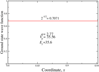
Figure 11: An outcome of the Mathematica 12 computation according to Ref. blinder . The rectangular double-well ground state function is fapp (for all practical purposes) constant and equal $1/\sqrt{2}$ in the interval $[-0,96,+0,96]$. Notice that $E-V_{0}=0.04>0$. Accordingly, within the employed numerical accuracy, the $+0.4$ detuning of $E$ from $V_{0}$ is insignificant as far as the shape (roughly constant) of the ground state function is concerned. A warning: we have not covered the full interval [-1,1], since the adopted numerical routine fails in the infinitesimal vicinity of the boundaries $\pm 1$.

In the considered case (data of Fig. 11), we deal with the following sequence of computed eigenvalues (we strictly observe conventions of Table I):

$E_{1}=35,6\to E_{0}=0,1974$	$E_{2}=36,1\to E_{1}=2,6647$	$E_{3}=37,8\to E_{2}=11.054$
$E_{4}=40,7\to E_{3}=25,1678$	$E_{5}=44,6\to E_{4}=44,61$	$E_{6}=49,7\to E_{5}=69,78$

Table 3: Rectangular double-well input: $a=2,77$, $V_{0}=35,56$.

This outcome needs to be compared with the second, $m=74$, row of Table II, where the eigenvalue (fapp !) $E_{0}=0$ has been omitted. Let us note that if we look seriously for the zero energy eigenfunction with the barrier height measure $V_{0}=35,56$, we need to deduce the corresponding value of $a=a(V_{0})$, by using Eq. (25). The result is $a=2,769$, hence encouragingly close to $a=2,77$.

To quantify the technical jeopardy of ”overshooting” the sharp eigenvalue zero by a small number, with obvious consequences for other computed eigenvalues, let us consider the reference data: $a=2,77$ and $V_{0}=36$. These strictly comply with the formulas (25), (26), and thus secure the existence of the eigenvalue zero for the ”renormalized” rectangular well Hamiltonian $\hat{H}_{ren}$, Eq. (28). Mathematica computation outcomes, while transformed according to the Table I give rise to (c.f. also Tables II and III):

$E_{1}=36\to E_{0}=0$	$E_{2}=36,5\to E_{1}=2,4674$	$E_{3}=38,2\to E_{2}=10.8565$
$E_{4}=41\to E_{3}=24,674$	$E_{5}=45\to E_{4}=44,4132$	$E_{6}=50,1\to E_{5}=69,58$

Table 4: Rectangular double-well input: $a=2,77$, $V_{0}=36$.

Let us indicate examples of rectangular double-well data, which imply the eigenvalue zero, and have the width parameter $a$ close to $a=2,77$. Exemplary cases read: $\{V_{0}=36,2,\,a=2,7724\},\{V_{0}=36,4,\,a=2,7734\},\{V_{0}=35,6,\,a=2,7693\}$. The fine tuning accuracy in Ref. blinder is up to two decimal digits.

IV.3 The concept of Neumann cut: Enforcing Neumann conditions at endpoints of the barrier.

We have mentioned before that the eigenvalue solution of the rectangular double-well problem, Section III.B, for $E\geq V_{0}$ involves the cosine function ($\cosh$ refers to tunneling solutions with $E\leq V_{0}$) within the internal barrier area. The continuity conditions at the barrier endpoints, connect derivatives of the cosine with sine tails, c.f. Eqs. (16) and (17), extending between the barrier and endpoints of the rectangular well support (i.e. either $\pm 1$ or $0$, $\pi$).

By examining Figs. 5, 6 and 7 (see e.g. also jph for a thorough discussion of the $\kappa_{m}=1$ case), we realize that although the Neumann condition is not realised at the internal barrier endpoints, it is worthwhile to consider (comparatively) a slight modification of the current best-fit procedure.

Namely, in addition to the standard Neumann well on $[-1,1]$, let us consider a cut-ff Neumann well, whose support is contracted from $[-1,1]$, to $[-1+2\triangle,1-2\triangle]$, with $\triangle=\triangle(m)$ evaluated for control values of $m=74,78,84,88,94$, for each predefined fitting procedure (location of superharmonic well minima and their distance from the interval $[-1,1]$ endpoints). First, for the case of $\kappa_{m}=m^{2}$, and next for $\kappa_{m}=m$.

So introduced narrowing of the original support $[-1,1]$ by $4\triangle$ (i.e. twice $2\triangle$) cut-off at the interval endpoints, defines the new re-sized Neumann well, which we call the Neumann cut.

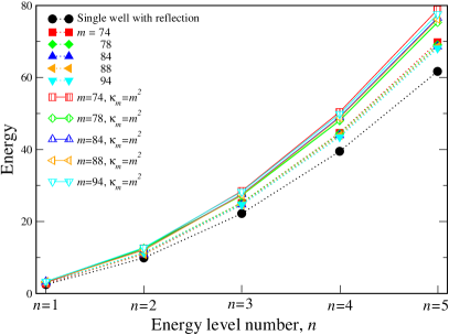
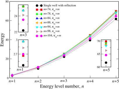
Figure 12: Left panel: we have filtered the spectral data to depict comparatively, (i) Neumann cut for $\kappa_{m}=m^{2}$ (top), (ii) best-fit rectangular well approximation of the superharmonic double-well for $\kappa_{m}=m^{2}$ (middle), (iii) Neumann well spectrum for $n>0$ (bottom). Right panel: A comparative display of, (i) Neumann cut for $\kappa_{m}=m$ (top data), (ii) Neumann well (single well with reflection) spectrum (bottom). Insets display a location of numerically retireved eigenvalues, up to $m=104$.

$m=94$	N-cut, $\kappa_{m}=m^{2}$	N-cut, $\kappa_{m}=m$	rect. well, $\kappa_{m}=m^{2}$	N-cut, $\kappa_{m}=m=98$	N-cut, $\kappa_{m}=m=104$	Neumann well
$E_{1}$	$3.273932$	$2.962383$	$>\,2.961\,>$	$2.830433$	$2.698934$	$2.4674$
$E_{2}$	$12.549520$	$11.3552029$	$>\,11.35\,>$	$11.3253029$	$11.294264$	$9.8696$
$E_{3}$	$27.281663$	$24.685528$	$>\,24.674\,>$	$24.109515$	$23.533541$	$22.2066$
$E_{4}$	$48.015727$	$43.446529$	$>\,43.4262\,>$	$42.254529$	$41.062529$	$39.4784$
$E_{5}$	$75.297125$	$68.131817$	$>\,68.10\,>$	$66.361801$	$64.591806$	$61.850$

Table 5: We depict positive ($E_{0}=0$ being kept in memory) eigenvalue data for the choice of $m=94$, for the following computation regimes: (i) Neumann cut (denoted N-cut) in the rectangular well approximation of the superharmonic double-well, $\kappa_{m}=m^{2}$; (ii) Neumann cut for $\kappa_{m}=m$, (iii) best-fit rectangular well approximation of the superharmonic double-well for $\kappa=m^{2}$, c.f. Table II and Fig. 10 (inequality symbols indicate lower and upper estimates provided respectively by the data (iv) and (ii)); (iv) standard Neumann well spectrum for $n>0$. Additionally, we have depicted two columns of data corresponding to $m=98$ and $m=104$, for the $\kappa_{m}=m$ Neumann cut.

For the record, we mention that the $m=104$ data, reported in Fig. 12 and Table IV, have been obtained through averaging over 15 repeated computation runs, with somewhat diverse outcomes. Effectively, the case of $m=104$ stays on the verge of Ref. blinder computing capabilities.

V Conclusions and contexts.

The major observation coming from our discussion in Section IV, stems from spectral data reported in Fig. 12 and Table IV. We have demonstrated that a numerical evaluation of lowest eigenvalues in the rectangular double-well approximation of the superharmonic double-well, for $\kappa_{m}=m^{2}$, $m=94$ is possible. The corresponding eigenfunctions (not depicted in the present paper) are retrievable as well. This in turn gives meaning to the spectral relaxation scenario of the original Smoluchowski process, in the least up to $m=104$.

The numerically retrieved spectral outcome can be effectively controlled and justified by two-sided estimates set by exact spectral solutions of two resized Neumann wells (Neumann cuts with $\kappa_{m}=m$). The pertinent Neumann cuts are set sharply upon interior barriers of rectangular double-well approximants, and effectively involve the validity on the Neumann condition at endpoints of resized support intervals. We point out that the Neumann cuts correspond to: (i) $\kappa_{m}=m=94$ (upper bound) and (ii) $\kappa_{m}=m=98$ (lower bound).

Our approximate solvability argument for the spectral problem of the superharmonic system $\hat{H}$ directly employs the ”renormalized” rectangular double well system $\hat{H}_{ren}=-(1/2)\Delta+[V(x)-V_{0}]$, where $V_{0}$ is the height of the double-well barrier ($-V_{0}$ measures the depth of local wells in the corresponding superharmonic double-well system). Therefore we are convinced that the approximation validity, as $m$ grows indefinitely, becomes questionable both on the formal and physical grounds. Our computation procedure (modulo the numerical programming adjustments) is operational for each finite value of $m<\infty$.

The presented analysis of a particular spectral problem for a superharmonic double-well Hamiltonian $\hat{H}$, Eq. (1), has been motivated by the method of eigenfunction expansions, often used in the analysis of spectral relaxation of diffusion processes, risken ; pavl ; jph . Somewhat surprisingly, the technical difficulty in solving this class of spectral problems is not exceptional, and is shared by a broad class of so called ”quasi-exactly solvable” Schrödinger systems, turbiner ; turbiner1 , see also baner ; brandon ; maiz ; okopinska . ”Quasi-solvability” is here a misnomer, because the solvability of the pertinent systems is not excluded, but extremally limited to some special cases.

The systems studied in Ref. turbiner are most easily constructed by means of the method employed in the present paper, where basically any positive $L^{2}(R)$-normalized function may serve as a square root of a certain probability distribution on $R$. A variety of Hamiltonian systems, with potentials of the generic form ${\cal{V}}(x)=[\Delta\rho_{*}^{1/2}(x)]/\rho_{*}^{1/2}(x)$ can be (re)constructed this way. In particular, the same route has been followed in Refs. streit ; zambrini ; vilela ; faris ; jph ; jph1 , while guided by the idea of ”reconstruction of (random) dynamics from the eigenstate”.

A peculiarity of all mentioned Schrödinger-type systems is that their ground state , by construction has been associated with the zero binding energy. Nonetheless, an issue of zero energy ground states is not anything close to being exotic. One may mention fairly serious research on bound states embedded in the continuum, and bound states with zero energy, lorinczi ; lorinczi1 ; lorinczi2 . Less mathematically advanced research concerning zero energy bound states can also be mentioned, nieto ; makowski ; robinett . This in line with a complementary resarch on zero-curvature eigenstates, ahmed ; gilbert1 .

The general issue of boundary conditions in case of impenetrable barriers, complementary to jph ; carlsaw , has been addressed in robinett ; karw ; diaz .

We point out that the Langevin-induced Fokker-Planck equations have been solved for potentials of the rectangular double-well shape, following risken ; kampen and kostin ; risken1 ; so . It might be of interest to investigate comparatively, Langevin-Fokker-Planck problems with drifts stemming (through negative gradients) from superharmonic double well potentials (3).

References

- (1) P. Garbaczewski and M. Żaba, ”Brownian motion in trapping enclosures: steep potential wells, bistable wells and false bistability of induced Feynman–Kac (well) potentials”, J. Phys. A: Math. Theor. 53 (31), 315001, (2020).
- (2) G. A. Pavliotis, Stochastic processes and applications, (Spriger, Berlin, 2014).
- (3) H. Risken, The Fokker-Planck equation, (Springer, Berlin, 1992).
- (4) S. Albeverio, R. Høegh-Krohn and L. Streit,” Energy forms, Hamiltonians, and distorted Brownian paths”, J. Math. Phys. 18, 907, (1977).
- (5) J. C. Zambrini, ”Stochastic mechanics according to E. Schrödinger”, Phys. Rev. A 33(3), 1532, (1986).
- (6) R. Vilela Mendes, ”Reconstruction of dynamics from an eigenstate”, J. Math. Phys., 27, 178, (1986).
- (7) W. G. Faris, ”Diffusive motion and where it leads”, in Diffusion, Quantum Theory and Radically Elementary Mathematics, edited by W. G. Faris (Princeton University Press, Princeton, 2006), pp. 1–43.
- (8) P. Garbaczewski, ”Probabilistic whereabouts of the ”quantum potential””, J. Phys.: Conf. Ser. 361, 012012, (2012).
- (9) A. V. Turbiner, ”One-dimensional quasi-exactly solvable Schrödinger equations”, Physics Reports, 642, 1, (2016).
- (10) A. Turbiner, ”Double Well Potential: Perturbation Theory, Tunneling, WKB (beyond instantons)”, Int. J. Mod. Phys. A 25, 647, (2010).
- (11) J.-L. Basdevant and J. Dalibard, ”Quantum mechanics”, (Springer, Berlin, 2002).
- (12) K. Banerjee and J. K. Bhattacharjee, ”Anharmonic oscillators and double wells: Closed-form global approximants for eigenvalues”, Phys. Rev. D 29, 1111, (1984).
- (13) D. Brandon and N. Saad, ”Exact and approximate solutions to Schrödinger’s equation with decatic potentials”, Open Physics, 11(3), 279, (2013).
- (14) F. Maiz et al., ”Sextic and decatic anharmonic oscillator potentials: Polynomial solutions”, Physica B 530, 101, (2018).
- (15) A. Okopińska, ”The Fokker-Planck equation for bistable potential in the optimized expansion”, Phys. Rev. E 65, 062101, (2002).
- (16) A. Dubkov and B. Spagnolo, ”Langevin approach to Lévy flights in fixed potentials: Exact results for stationary probability distributions”, Acta Phys Pol. B 38, 1745, (2007).
- (17) A. A. Kharcheva et al, ”Spectral characteristics of steady-state Lévy flights in confinement potential profiles”, J. Stat. Mech. (2016) 054039.
- (18) R. Toenjes R, I. M. Sokolov and E. B. Postnikov, ”Nonspectral relaxation in one-dimensional Ornstein–Uhlenbeck process”, Phys. Rev. Lett. 110, 150602, (2013).
- (19) N. G. van Kampen, ”A soluble model for diffusion in a bistable potential”, J. Stat. Phys. 17, 71, (1977).
- (20) R. S. Larson and M. D, Kostin, ”Kramers theory of chemical kinetics: Eigenvalues and eigenfunction analysis”, J. Chem. Phys, 69,4821, (1978).
- (21) M. Mörsch, H. Risken and H. D. Vollmer, ”One-dimensional diffusion in a soluble model potential”, Z. Physik B 32, 245, (1979).
- (22) F. So and K. L. Liu, ”A study of the Fokker-Planck equation of bistable systems by the method of state-dependent diagonalization”, Physica A 277, 335, (2000).
- (23) S. M. Blinder, ”Exact Solution for Rectangular Double-Well Potential”, Wolfram Demonstrations Project, (2013), http://demonstrations.wolfram.com/ExactSolutionForRectangularDoubleWellPotential/
- (24) E. Peacock-Lȯpez, ”Exact Solutions of the Quantum Double-Square-Well Potential”, Chem. Educator, 2006, 11, 383-393.
- (25) V. Jelic and F. Marsiglio, ”The double well potential in quantum mechanics: a simple, numerically exact formulation”, Eur. J. Phys. 33, 1651, (2012).
- (26) B. Dybiec et al., ”Lévy flights versus Lévy walks in bounded domains”, Phys. Rev. E95, 052102, (2017).
- (27) B. Dybiec, E. Gudowska-Nowak and P. Hänggi, ”Lévy-Brownian motion on finite intervals: Mean first passage analysis”, Phys. Rev. E 73, 046104, (2006).
- (28) V. Linetsky, ”On the transition densities for reflected diffusions”, Adv. App. Prob. 37, 435-460, (2005).
- (29) T. Bickel, ”A note on confined diffusion”, Physica A 377, 24-32, (2007).
- (30) H. S. Carlsaw and J. C. Jaeger, Conduction of Heat in Solids, (Oxford University Press, London, 1959).
- (31) A. Pilipenko, An introduction to stochastic differential equations with reflection, (Potsdam University Press, Potsdam, 2014).
- (32) M. Kuczma, 2009 An Introduction to the Theory of Functional Equations and Inequalities, (Birkhäuser, Basel, 2009).
- (33) J. Lőrinczi, F. Hiroshima and V. Betz, Feynman–Kac-Type Theorems and Gibbs Measures on Path Space, (De Gruyter Studies in Mathematics vol 34) (De Gruyter, Berlin, 2020)
- (34) K. Kaleta and J. Lőrinczi, ”Zero-energy bound state decay for non-local Schrödinger Operators”, Commun. Math. Phys. 374(3), 2151, (2020).
- (35) G. Ascione and J. Lőrinczi, ”Potentials for non-local Schrödinger operators with zero eigenvalues”, arXiv:2005.138881, (2020)
- (36) J. Daboul and M. M. Nieto, ”Quantum bound states with zero binding energy”, Phys. Lett. A 190, 357, (1994).
- (37) A. J. Makowski, ”Exact, zero-energy, square-integrable solutions of a model related to the Maxwell’s fish-eye problem”, Ann. Phys. 324, 2465, (2009).
- (38) L. P. Gilbert et al, ”Playing quantum physics jeopardy with zero-energy eigenstate”, Am. J. Phys. 74, 1035, (2006).
- (39) Z. Ahmed and S. Kesari, ”The simplest model of the zero curvature eigenstate”, Eur. J. Phys.35,018002, (2014).
- (40) L. P. Gilbert et al., ”More on the asymmetric infinite square well: energy eigenstates with zero curvature”, Eur. J. Phys. 26, 815, (2005).
- (41) M. Belloni and R. W. Robinett, ”The infinite well and Dirac delta function potentials as pedagogical, mathematical and physical models in quantum mechanics”, Physics Reports, 540, 24, (2014).
- (42) P. Garbaczewski and. Karwowski, ”Impenetrable barriers and canonical quantization”, Am. J. Phys. 72, 924, (2004).
- (43) J. I. Diaz, ”On the ambiguous treatment of the Schrödinger equation for the infinite potential well and an alternative via flat solutions: The one-dimensional case”, Interfaces and Free Boundaries 17(3),333, (2015)
- (44) R. S. Larson and M. D. Kostin, ”Kramers theory of chemical kinetics: Eigenvalues and eigenfunction analysis” J. Chem. Phys. 69, 4821, (1978)
- (45) F. So and K. L. Liu, ”A study of the Fokker–Planck equation of bistable systems by the method of state-dependent diagonalization”, Physica A 277, 335, (2000)