Suboptimal coverings for continuous spaces of control tasks

Abstract

We propose the $\alpha$-suboptimal covering number to characterize multi-task control problems where the set of dynamical systems and/or cost functions is infinite, analogous to the cardinality of finite task sets. This notion may help quantify the function class expressiveness needed to represent a good multi-task policy, which is important for learning-based control methods that use parameterized function approximation. We study suboptimal covering numbers for linear dynamical systems with quadratic cost (LQR problems) and construct a class of multi-task LQR problems amenable to analysis. For the scalar case, we show logarithmic dependence on the “breadth” of the space. For the matrix case, we present experiments 1) measuring the efficiency of a particular constructive cover, and 2) visualizing the behavior of two candidate systems for the lower bound.

1 Introduction

An advanced control system such as a mobile robot may be required to perform many different tasks. If the task set is finite, like selecting between “map an environment” and “deliver a package”, then its size is naturally quantified by the number of tasks. If the task set is infinite, like delivering packages with arbitrary mass and inertial properties, then its size is not so easily quantified. Even if the task space is equipped with a metric or measure, these structures may be only weakly linked to the diversity of behavior required for good performance on all tasks.

Our interest in this issue is motivated by multi-task paradigms in learning-based control, where the policy is selected from a parameterized family of functions that map state and task parameters directly to actions. As the task space expands from a singleton set, we expect to need a more expressive class of functions to represent a good multi-task policy. In this work, we propose the $\alpha$-suboptimal covering number to capture this idea. For a task space $\Phi$ and a suboptimality ratio $\alpha>1$, we define $N_{\alpha}(\Phi)$ as the size of the smallest set of single-task policies $\mathcal{C}$ such that for every $\phi\in\Phi$, at least one $\pi\in\mathcal{C}$ has a cost ratio no greater than $\alpha$ relative to the optimal policy for $\phi$. If the policies in $\mathcal{C}$ are parameterized functions, then $\mathcal{C}$ provides an upper bound on the number of parameters needed to represent an $\alpha$-suboptimal multi-task policy. In switching-based adaptive control, where $\phi$ is unknown, a smaller $\mathcal{C}$ implies a faster convergence time.

To study suboptimal covering numbers in a concrete setting, we consider linear dynamical systems with quadratic cost functions, or LQR problems. LQR problems are a common setting to analyze learning algorithms because detailed properties are known (Fazel et al., 2018, for example). This has led to new inquiries into their fundamental properties (Bu et al., 2019). We construct a family of well-behaved multi-task LQR problems where $\Phi$ is controlled by a “breadth” parameter $\theta\in[1,\infty)$, and for which $N_{\alpha}(\Phi_{\theta})$ is finite and increasing in $\theta$. For the special case of a scalar LQR problem, we derive matching logarithmic upper and lower bounds on $N_{\alpha}(\Phi_{\theta})$ as a function of $\theta$. As an effort towards analogous bounds for the matrix case, we present empirical results intended to shed light on the problem structure. For the upper bound, we analyze properties of a logical extension of our scalar cover. For the lower bound, we visualize suboptimal neighborhoods for two choices of “extremal” systems and find surprising topological behavior for one choice.

This paper is an initial step towards a comprehensive theory. In addition to a more complete picture of deterministic LQR systems, ideas of $\alpha$-suboptimal coverings could be applied to a wide range of multi-task problems. We also hope they will lead to insights about function class expressiveness in learning-based multi-task control.

2 Problem setting

In this section, we first define suboptimal covering numbers with respect to an abstract multi-task control problem independent of distinctions such as continuous vs. discrete time and stochastic vs. deterministic. We then instantiate these notions for a particular class of LQR problems.

Notation

The set of all functions $\mathcal{X}\mapsto\mathcal{Y}$ is denoted by $\mathcal{Y}^{\mathcal{X}}$. The relation $A\succeq B$ (resp. ${A\succ B}$) denotes that $A-B$ is positive semidefinite (resp. definite). Matrices of zeros and ones, with dimension implied by context, are denoted by $\mathbf{0}$ and $\mathbf{1}$. The integers $\{1,\dots,N\}$ are denoted by $[N]$.

Multi-task optimal control

A multi-task optimal control problem is defined by an arbitrary state space $\mathcal{X}$, action space $\mathcal{U}$, and task space $\Phi$; a class of reference policies $\Pi_{\mathrm{ref}}\subseteq\mathcal{U}^{\mathcal{X}}$, and a strictly positive objective function $J:\Phi\times\mathcal{U}^{\mathcal{X}}\mapsto\mathbb{R}_{>0}$. The partial application of $J$ for $\phi\in\Phi$ is denoted by $J_{\phi}:\mathcal{U}^{\mathcal{X}}\mapsto\mathbb{R}$. The optimal reference cost for an task is denoted by $J^{\star}_{\phi}=\min_{\pi\in\Pi_{\mathrm{ref}}}J_{\phi}(\pi)$.

Suboptimal coverings

Consider a multi-task optimal control problem $(\mathcal{X},\mathcal{U},\Phi,\Pi_{\mathrm{ref}})$ and a suboptimality ratio $\alpha>1$. The $\alpha$-suboptimal neighborhood of the policy $\pi:\mathcal{X}\mapsto\mathcal{U}$ is $\mathscr{N}_{\alpha}(\pi)=\left\{\phi\in\Phi:\left.J_{\phi}(\pi)\middle/J^{\star}_{\phi}\right.\leq\alpha\right\}.$ The set $\mathcal{C}\subseteq\mathcal{U}^{\mathcal{X}}$ is an $\alpha$-suboptimal cover of $\ \Phi$ if $\ \bigcup_{\pi\in\mathcal{C}}\mathscr{N}_{\alpha}(\pi)=\Phi.$ The $\alpha$-suboptimal covering number of $\Phi$, denoted $N_{\alpha}(\Phi)$, is the size of the smallest finite $\alpha$-suboptimal cover of $\Phi$ if one exists, or $\infty$ otherwise.

Standard LQR problem

A continuous-time, deterministic, infinite-horizon, time-invariant LQR problem with full-state feedback is defined by state space $\mathcal{X}=\mathbb{R}^{n}$, action space $\mathcal{U}=\mathbb{R}^{m}$, linear dynamics $\dot{x}=Ax+Bu,$ where $A\in\mathbb{R}^{n\times n},\ B\in\mathbb{R}^{n\times m}$, and quadratic cost

$$J(\pi)=\operatorname*{\mathbb{E}}_{x(0)\sim\operatorname{\mathcal{N}}(\mathbf{0},I)}\int_{0}^{\infty}\big{(}x^{\top}Qx+u^{\top}Ru\big{)}\,\mathrm{d}t,$$

where $Q\succeq\mathbf{0}$ and $R\succ\mathbf{0}$ are cost matrices of appropriate dimensions and $\operatorname{\mathcal{N}}(\mathbf{0},I)$ is the unit Gaussian distribution. For the purposes of this paper, the pair $(A,B)$ is controllable if $J(\pi)<\infty$ for some policy $\pi$. If $(A,B)$ is controllable, then the optimal policy is the linear $u=K^{\star}x$, where $K^{\star}\in\mathbb{R}^{m\times n}$ can be computed by finding the unique maximal positive semidefinite solution $P$ of the algebraic Riccati equation $A^{\top}P+PA-PBR^{-1}B^{\top}P+Q=\mathbf{0}$ (henceforth called the maximal solution) and letting $K^{\star}=-R^{-1}B^{\top}P$ (Kalman, 1960). Additionally, $J(K^{\star})=\mathrm{Tr}\left[P\right]$. An arbitrary controller $K\in\mathbb{R}^{m\times n}$ is stabilizing if $J(K)<\infty$, in which case $J(K)$ satisfies

$$J(K)=\mathrm{Tr}\left[(Q+K^{\top}RK)W\right]\!,\ \text{where}\ \ W=\int_{0}^{\infty}{e^{t(A+BK)}}^{\top}{e^{t(A+BK)}}dt.$$ (1)

$W$ can be computed by solving the Lyapunov equation $(A+BK)^{\top}W+W(A+BK)+I=\mathbf{0}.$

Multi-dynamics LQR

A fully general formulation of multi-task LQR would allow variations in each of $(A,B,Q,R)$, but this creates redundancy. Any LQR problem where $Q\succ 0$ is equivalent via change of coordinates to another LQR problem where $Q=I$ and $R=I$. To reduce redundancy, we consider only multi-dynamics LQR problems where $Q=I_{n\times n}$ and $R=I_{m\times m}$ in this work. The reference policy class is linear: $\Pi_{\mathrm{ref}}=\mathbb{R}^{m\times n}$.

A multi-dynamics LQR problem can be defined by $\Phi=\mathbf{A}\times\mathbf{B}$ for some sets $\mathbf{A}\subseteq\mathbb{R}^{n\times n}$ and ${\mathbf{B}\subseteq\mathbb{R}^{n\times m}}$, but it is not obvious how to design $\mathbf{A}$ and $\mathbf{B}$. To support an asymptotic analysis of $N_{\alpha}(\Phi)$, the task space $\Phi$ should have a real-valued “breadth” parameter $\theta$ that sweeps from a single task to sets with arbitrarily large, but finite, covering numbers. Matrix norm balls are a popular representation of dynamics uncertainty in the robust control literature, but they can easily contain uncontrollable pairs, and removing the uncontrollable pairs can lead to an infinite covering number. For example, in the scalar problem $\mathbf{A}=\{a\},\ \mathbf{B}=[-\theta,0)\cup(0,\theta]$, where $a>0$, it can be shown that no $\alpha$-suboptimal cover is finite.

These properties are worrying, but the example $\mathbf{B}$ is pathological. The zero crossing is analogous to reversing the direction of force applied by an actuator in a physical system. A more relevant multi-dynamics problem is variations in mass or actuator strength, whose signs are fixed. We formalize this idea with the following definition.

Decomposed dynamics form

Fix $A\in\mathbb{R}^{n\times n}$ and a breadth parameter $\theta\geq 1$. Let $\mathbf{B}=\{U\Sigma V^{\top}:\Sigma\in\boldsymbol{\Sigma}\}$, where $\boldsymbol{\Sigma}=\{\operatorname{diag}(\sigma):\sigma\in[\frac{1}{\theta},1]^{d}\}$. The matrices $U\in\mathbb{R}^{n\times d}$ and $V\in\mathbb{R}^{m\times d}$ each have rank $d$, where $0<d\leq\min\{n,m\}$. The tuple $(A,U,V,\theta)$ fully defines a multi-task LQR problem in decomposed dynamics form, or DDF problem for brevity.

The continuity of the LQR cost (1) with respect to $B$ and the compactness of $\Phi$ for any $\theta$ imply that $N_{\alpha}(\Phi_{\theta})$ is always finite. Variations in $A$ are redundant in the scalar case where we focus our theoretical work in this paper. The definition can be extended to include them in future work.

Linearized quadrotor example

As an example of a realistic DDF problem, we consider the quadrotor helicopter illustrated in Figure 1. Near the hover state, its full nonlinear dynamics are well approximated by a linearization. The state is given by $x=(\mathbf{x},\mathbf{v},\mathbf{r},\boldsymbol{\omega}),$ where $\mathbf{x}\in\mathbb{R}^{3}$ is position, $\mathbf{v}\in\mathbb{R}^{3}$ is linear velocity, $\mathbf{r}\in\mathbb{R}^{3}$ is attitude Euler angles, and $\boldsymbol{\omega}\in\mathbb{R}^{3}$ is angular velocity. The inputs $u\in\mathbb{R}^{4}_{\geq 0}$ are the squared angular velocities of the propellers.

Many factors influence the response to inputs, including geometry, mass, moments of inertia, motor properties, and propeller aerodynamics. These can be combined and partially nondimensionalized into four control authority parameters to form $\phi\in\Phi$. The hover state occurs at $x=\mathbf{0},\ u\propto\mathbf{1}$, where the constant input counteracts gravity. The linearized dynamics are given by

$$\dot{x}=\underbrace{\begin{bmatrix}\mathbf{0}&I&\mathbf{0}&\mathbf{0}\\ \mathbf{0}&\mathbf{0}&G&\mathbf{0}\\ \mathbf{0}&\mathbf{0}&\mathbf{0}&I\\ \mathbf{0}&\mathbf{0}&\mathbf{0}&\mathbf{0}\\ \end{bmatrix}}_{A}x+\underbrace{\begin{bmatrix}\mathbf{0}&\mathbf{0}\\ \hat{e}_{z}&\mathbf{0}\\ \mathbf{0}&\mathbf{0}\\ \mathbf{0}&I\\ \end{bmatrix}}_{U}\underbrace{\begin{bmatrix}\sigma_{z}&&&\\ &\sigma_{\phi}&&\\ &&\sigma_{\theta}&\\ &&&\sigma_{\psi}\\ \end{bmatrix}}_{\Sigma}\underbrace{\begin{bmatrix}[r]1&1&1&1\\ 1&-1&-1&1\\ -1&-1&1&1\\ 1&-1&1&-1\\ \end{bmatrix}}_{V^{\top}}u,\quad G=\begin{bmatrix}[r]0&g&0\\ -g&0&0\\ 0&0&0\\ \end{bmatrix},$$

where $g$ is the gravitational constant and $\hat{e}_{z}=[0\ 0\ 1]^{\top}$. The parameters $(\sigma_{z},\ \sigma_{\phi},\ \sigma_{\theta},\ \sigma_{\psi})$ denote the thrust, roll, pitch, and yaw authority constants respectively. Since we use the convention $\sigma\in[\frac{1}{\theta},1]$, the maximum value of each constant can be varied by scaling the columns of $U$.

Figure 1: Quadrotor helicopter with position states $x,y,z$, attitude states $\phi,\theta,\psi$, and propeller speed inputs $u_{1},u_{2},u_{3},u_{4}$. The linearized dynamics at hover, subject to variations in mass, geometry, etc., can be expressed in decomposed dynamics form—see Section 2.

3 Theoretical results

In this section we show logarithmic upper and lower bounds on the growth of $N_{\alpha}(\Phi_{\theta})$ in $\theta$ for scalar DDF problems. We present several intermediate results in matrix form because they are needed for our empirical results later. We begin with a key lemma in the framework of guaranteed cost control (GCC) from Petersen and McFarlane (1994), simplified for our use case.

Lemma 3.1 (GCC synthesis, Petersen and McFarlane (1994)).

Given the multi-task LQR problem $\mathbf{A}=\{A\}$, $\mathbf{B}=\{B_{1}\Delta+B_{2}:\lVert\Delta\rVert\leq 1\}$, where $B_{1},B_{2}\in\mathbb{R}^{m\times p}$ are arbitrary for arbitrary $p$, and the state cost matrix is $Q\succ\mathbf{0}$, if there exists $\tau>0$ such that $P\succ\mathbf{0}$ solves the Riccati equation

$$A^{\top}P+PA+P\left(\textstyle\frac{1}{\tau}B_{1}B_{1}^{\top}-\frac{1}{1+\tau}B_{2}B_{2}^{\top}\right)P+Q=\mathbf{0},$$ (2)

then the controller $K=-\frac{1}{1+\tau}B_{2}^{\top}P$ has cost $J_{B}(K)\leq\mathrm{Tr}\left[P\right]$ for all $B\in\mathbf{B}$. Also, $\mathrm{Tr}\left[P\right]$ is a convex function of $\tau$.

We use the notation $P,\tau,K={\texttt{GCC}}(A,B_{1},B_{2},Q)$ to indicate that $P,\tau$ solve (2) and $K$ is the corresponding controller. It is straightforward to show that any DDF problem can be expressed in the form required by lem:petersen-gcc with additional constraints on $\Delta$.

In the original presentation, Petersen and McFarlane (1994) treat $B_{1}$ as given, so they accept that (2) may have no solution (for example, when $A=2I,B_{1}=I,B_{2}=\mathbf{0}$). Our application requires constructing values of $B_{1},B_{2}$ that guarantee a solution, motivating the following lemma. We abbreviate the reference text Lancaster and Rodman (1995) as Lan95.

Lemma 3.2 (existence of $\alpha$-suboptimal GCC).

For the DDF problem $(A,U,V,\theta)$, if $B\in\mathbf{B}$ and $\alpha>1$, then there exists $B_{1}\neq\mathbf{0}\in\mathbb{R}^{m\times n}$ such that the GCC Riccati equation (2) with $B_{2}=B$ has a solution $(P,\tau)$ satisfying $\mathrm{Tr}\left[P\right]\leq\alpha J^{\star}_{B}$.

Proof 3.3.

For this proof, it will be more convenient to write the algebraic Riccati equation as

$$A^{\top}P+PA-PDP+Q=\mathbf{0},$$ (3)

where $D\succeq\mathbf{0}$. Let $\mathcal{D}=\{D\succeq\mathbf{0}:(A,D)\ \text{ is controllable}\}$. Controllability of $(A,B)$ implies that $BB^{\top}\in\mathcal{D}\$ (Corollary 4.1.3 Lan95). Let $\mathrm{Ric}_{+}$ denote the map from $\mathcal{D}$ to the maximal solution of (3), which is continuous (Theorem 11.2.1 Lan95), and let $\mathcal{D}_{\alpha}=\{D\in\mathcal{D}:\mathrm{Tr}\left[\mathrm{Ric}_{+}(D)\right]<\alpha J^{\star}_{B}\}$. The set $\mathcal{D}_{\alpha}$ is open in $\mathcal{D}$ by continuity and is nonempty because it contains $BB^{\top}$. Now define $B_{1}(\tau)=\tau B$ for $\tau\in(0,\frac{1}{2})$. The equivalent of $D$ in the GCC Riccati equation (2) becomes

$$\textstyle D(\tau)=-\frac{1}{\tau}B_{1}(\tau)B_{1}(\tau)^{\top}+\frac{1}{1+\tau}B_{2}B_{2}^{\top}=\frac{1-\tau-\tau^{2}}{1+\tau}BB^{\top}.$$

As a positive multiple of $BB^{\top}$, we know $D(\tau)\in\mathcal{D}$, and because $\lim_{\tau\to 0}D(\tau)=BB^{\top}$, the set of $\tau$ for which $D(\tau)\in\mathcal{D}_{\alpha}$ is nonempty. Any such $\tau$ and $B_{1}(\tau)$ provide a solution.

Finally, the following comparison result will be useful in several places.

Lemma 3.4 (Lan95, Corollary 9.1.6).

Given two algebraic Riccati equations

$$A^{\top}P+PA-PBB^{\top}P+Q=\mathbf{0}\quad\text{ and }\quad\tilde{A}^{\top}P+P\tilde{A}-P\tilde{B}\tilde{B}^{\top}P+\tilde{Q}=\mathbf{0},$$

with maximal solutions $P$ and $\tilde{P}$, let $X=\begin{bmatrix}Q&A^{\top}\\ A&-BB^{\top}\end{bmatrix}$ and $\tilde{X}=\begin{bmatrix}\tilde{Q}&\tilde{A}^{\top}\\ \tilde{A}&-\tilde{B}\tilde{B}^{\top}\end{bmatrix}$. If $X\!\succeq\!\tilde{X}$, then $P\!\succeq\!\tilde{P}$.

3.1 Scalar upper bound

We are now ready to bound the covering number for scalar systems. The first lemma bounding $J^{\star}_{a,b}$ will be useful for the lower bound also. We then construct a cover inductively.

Lemma 3.5.

In a scalar LQR problem, if $a>0$ and $0<b\leq 1$, then the optimal scalar LQR cost satisfies the bounds $\left.2a\middle/b^{2}\right.<J^{\star}_{a,b}<\left.(2a+1)\middle/b^{2}\right..$

Proof 3.6.

The lower bound is visible from the closed-form solution for the scalar Riccati equation, which is $J^{\star}_{a,b}=\frac{a+\sqrt{a^{2}+b^{2}}}{b^{2}}.$ The upper bound is obtained by substituting $a^{2}+b^{2}\leq(a+1)^{2}$.

Lemma 3.7.

If $p,\tau,k={\texttt{GCC}}(a,b_{1},b_{2},q)$, then for any $\beta\in(0,1)$, there exists $k^{\prime}\in\mathbb{R}$ such that $\displaystyle p^{\prime},\tau,k^{\prime}={\texttt{GCC}}\left(a,\beta b_{1},\beta b_{2},\beta^{-2}q\right)$, where $\ p^{\prime}=\beta^{-2}p$.

Proof 3.8.

In the scalar system, the GCC matrix Riccati equation (2) reduces to the quadratic equation

$$\left(\textstyle\frac{1}{\tau}b_{1}^{2}-\frac{1}{1+\tau}b_{2}^{2}\right)p^{2}+2ap+q=0.$$ (4)

Substituting $p^{\prime}=\beta^{-2}p$ into (4) and multiplying by $\beta^{-2}$ yields a new instance of (4) with the parameters $b_{1}^{\prime}=\beta b_{1}$,  $b_{2}^{\prime}=\beta b_{2}$,  $q^{\prime}=\beta^{-2}q$, for which $p^{\prime}$ is a solution with $\tau$ unchanged.

Theorem 3.9.

For the scalar DDF problem defined by $\mathbf{A}=\{a\}$, where $a>0$, and $\mathbf{B}=\left[\textstyle\frac{1}{\theta},1\right]$, if $\alpha\geq\frac{2a+1}{2a}$, then $N_{\alpha}(\mathbf{B})=O(\log\theta)$.

Proof 3.10.

We construct a cover from the upper end of $\mathbf{B}$. By lem:scalar-cost-ub, the condition ${\alpha\geq\frac{2a+1}{2a}}$ implies that $J^{\star}_{b=1}<\alpha 2a<\alpha J^{\star}_{b=1}.$ Therefore, by lem:petersen-gcc,lem:petersen-existence, there exists $\beta\in(0,1)$ and $p,\tau,k$ such that $p,\tau,k={\texttt{GCC}}(a,(1-\beta)/2,(1+\beta)/2,1)$ and $p\leq\alpha 2a$.

Proceeding inductively, suppose that for $N\geq 1$, we have covered $[\beta^{N},1]$ by the intervals $\mathbf{B}_{n}=[\beta^{n+1},\beta^{n}]$ for $n\in\{0,\dots,N-1\}$, and each $\mathbf{B}_{n}$ has a controller $k_{n}$ such that

$$\beta^{-2n}p,\tau,k_{n}={\texttt{GCC}}\left(a,\left.(\beta^{n}-\beta^{n+1})\middle/2\right.,\left.(\beta^{n}+\beta^{n+1})\middle/2\right.,\beta^{-2n}\right).$$

Then the existence of the desired $\mathbf{B}_{N},k_{N}$ follows immediately from lem:scalar-cover-recursion.

By lem:lancaster-ARE-domination, for each $\mathbf{B}_{n}$ the GCC state cost $q_{n}=\beta^{-2n}\geq 1$ is an upper bound on the cost if we replace $q_{n}$ with $1$ to match the DDF problem. Therefore, for each interval $\mathbf{B}_{n}$, for all $b\in\mathbf{B}_{n}$,

$$\alpha J^{\star}_{b}\geq\alpha J^{\star}_{\beta^{n}}>\beta^{-2n}\alpha 2a\geq\beta^{-2n}p\geq J_{b}(k_{n}),$$

where first inequality is due to lem:lancaster-ARE-domination, the second is due to lem:scalar-cost-ub, the third is by construction of $p$, and last is due to the GCC guarantee of $k_{n}$. Hence, $\mathbf{B}_{n}\subseteq\mathscr{N}_{\alpha}(k_{n})$. We cover the full $\mathbf{B}$ when $\beta^{N}\leq\frac{1}{\theta}$, which is satisfied by $N\geq-\log\theta/\log\beta$.

3.2 Scalar lower bound

For the matching lower bound, we begin by deriving a simplified overestimate of $\mathscr{N}_{\alpha}(k)$. We then show that the true $\mathscr{N}_{\alpha}(k)$ is still a closed interval moving monotonically with $k$. Finally, we argue that the gaps between consecutive elements of a cover grow at most geometrically, while the range of $k$ values in a cover must grow linearly with $\theta$.

Lemma 3.11.

For a scalar DDF problem with $a\geq 1,\ \mathbf{B}=[\frac{1}{\theta},1]$, for any $k<0$, if $\alpha\geq 3/2$, then $\mathscr{N}_{\alpha}(k)\subseteq\frac{1}{|k|}[c_{1}\!-\!c_{2},\ c_{1}\!+\!c_{2}]$, where $c_{1}$ and $c_{2}$ are constants depending on $\alpha$ and $a$.

Proof 3.12.

Beginning with the closed-form solution for $J_{b}(k)$, which can be derived from (1), we define

$$J_{b}(k)=\frac{1+k^{2}}{-2(a+bk)}\geq\frac{k^{2}}{-2(a+bk)}\triangleq\underline{J_{b}}(k).$$ (5)

By lem:scalar-cost-ub, we have $J^{\star}_{b}<\left.3a\middle/b^{2}\right.\triangleq\overline{J^{\star}_{b}}$, so $\tilde{r}=\left.\underline{J_{b}}(k)\middle/\,\overline{J^{\star}_{b}}\right.$ is a lower bound on the suboptimality of $k$. Computing $\partial^{2}\tilde{r}/\partial b^{2}$ shows that $\tilde{r}$ is strictly convex in $b$ on the domain $a+bk<0$, so the $\alpha$-sublevel set of $\tilde{r}$ is the closed interval with boundaries where $\tilde{r}=\alpha$. This equation is quadratic in $b$ with the solutions $b=-a(3\alpha\pm\sqrt{9\alpha^{2}-6\alpha})/k$. The resulting interval contains $\mathscr{N}_{\alpha}(k)$.

Lemma 3.13

For a scalar DDF problem, if $\alpha>1$ and $k<-1$, then $\mathscr{N}_{\alpha}(k)$ is either empty or a closed interval $[b_{1},b_{2}]$, with $b_{1}$ and $b_{2}$ positive and nondecreasing in $k$.

Proof 3.14.

The result follows from quasiconvexity of both the suboptimality ratio $J_{b}(k)/J^{\star}_{b}$ and the cost $J_{b}(k)$. Showing these requires some tedious calculations. For details, see Appendix A.

Theorem 3.15.

For a scalar DDF problem with $a=1,\ \mathbf{B}=[\frac{1}{\theta},1]$, if $\alpha\geq\frac{3}{2}$, then $N_{\alpha}(\mathbf{B})=\Omega(\log\theta)$.

Proof 3.16.

From the closed-form solution $k^{\star}_{a,b}=-(a+\sqrt{a^{2}+b^{2}})/b$, we observe that $k^{\star}_{b}<-1$ for all $b\in\mathbf{B}$. This, along with the quasiconvexity of $J_{b}(k)$ in $k$, implies that there exists a minimal $\alpha$-suboptimal cover $\mathcal{C}$ for which all $k_{i}<-1$. Suppose $\mathcal{C}=k_{1},\dots,k_{N}$ is such a cover, ordered such that $k_{i}<k_{i+1}$. Then by lem:subopt-convex, $\mathscr{N}_{\alpha}(k_{i})$ and $\mathscr{N}_{\alpha}(k_{i+1})$ must intersect, so their overestimates according to lem:scalar-neighborhood-optimistic certainly intersect, therefore satisfying

$$\frac{c_{1}+c_{2}}{-k_{i+1}}\geq\frac{c_{1}-c_{2}}{-k_{i}}\implies\frac{k_{i+1}}{k_{i}}\leq\frac{c_{1}+c_{2}}{c_{1}-c_{2}}\implies\frac{k_{N}}{k_{1}}\leq\left(\frac{c_{1}+c_{2}}{c_{1}-c_{2}}\right)^{N-1}.$$

By lem:scalar-neighborhood-optimistic, to cover $b=1$ controller $k_{1}$ must satisfy $k_{1}\geq-(c_{1}+c_{2})$, and to cover $b=\frac{1}{\theta}$, controller $k_{N}$ must satisfy $k_{N}\leq-\theta(c_{1}-c_{2})$. Along with the previous result, this implies

$$\left(\frac{c_{1}+c_{2}}{c_{1}-c_{2}}\right)^{N-1}\geq\theta\frac{c_{1}-c_{2}}{c_{1}+c_{2}}\implies N\geq\frac{\log\theta}{\log\frac{c_{1}+c_{2}}{c_{1}-c_{2}}}.$$

Recalling that $c_{1}$ and $c_{2}$ only depend on $a$ and $\alpha$, the $\Omega(\log\theta)$ dependence on $\theta$ is established.

Remarks

• For the upper bound, it may be possible to compute or bound $\beta$ in the scalar case as a function of $a$ and $\alpha$, but the analogous result will likely be much more complicated in the matrix case.

• thm:covering-scalar imposes a lower bound on $\alpha$ greater than $1$. We believe this is a mild condition in practice: if the application demands a suboptimality ratio very close to 1, then the size of the suboptimal cover is likely to become impractical for storage. However, further theoretical results building upon suboptimal coverings may require eliminating the bound.

4 Empirical results

For matrix DDF problems, we present empirical results as a first step towards covering number bounds. We begin by testing a cover construction. If the construction fails to achieve a conjectured upper bound in a numerical experiment, then either the conjecture is false, or the construction is not efficient. A natural idea is to extend the geometrically spaced sequence of $b$ values from lem:scalar-cost-ub to multiple dimensions. We now make this notion, illustrated in Figure 2, precise.

Definition 4.1 (Geometric grid partition).

Given a DDF problem with $\boldsymbol{\Sigma}=[\frac{1}{\theta},1]^{d}$, and a grid pitch $k\in\mathbb{N}_{+}$, select $s_{1},\dots,s_{k+1}$ such that $s_{1}=\frac{1}{\theta}$, $s_{k+1}=1$, and $\frac{s_{i+1}}{s_{i}}>0$ is constant. For each $j\in[k]^{d}$, define the grid cell $\boldsymbol{\Sigma}(j)=\textstyle\prod_{i=1}^{d}[s_{j(i)},s_{j(i)+1}],$ where $j(i)$ is the $i^{\mathrm{th}}$ component of $j$. The cells satisfy $\boldsymbol{\Sigma}=\textstyle\bigcup_{j\in[k]^{d}}\boldsymbol{\Sigma}(j),$ thus forming an partition (up to boundaries) of $\boldsymbol{\Sigma}$ into $k^{d}$ cells.

   

Figure 2: Application of geometric grid cover to linearized quadrotor. (a) Illustration of geometric grid partition. (b) Empirical upper bound on covering number. (c) Suboptimality ratios for corner cells in empirical cover. Discussion in Section 4.

Empirical upper bound on $N_{\alpha}(\Phi)$.

In this experiment, we construct an $\alpha$-suboptimal cover $\mathcal{C}$ using geometric grids, such that each $K\in\mathcal{C}$ is $\alpha$-suboptimal for a full grid cell. For each cell $\boldsymbol{\Sigma}(j)$, we attempt GCC synthesis. If it succeeds, we check if $\boldsymbol{\Sigma}(j)\subseteq\mathscr{N}_{\alpha}(K(j))$. If not, we increment the grid pitch $k$ and try again. Termination is guaranteed by continuity. We show results for the linearized quadrotor with $\alpha=2$ in Figure 2. The data follow roughly logarithmic growth, as indicated by the linear least-squares best-fit curve in black. Small values of $\theta$ are excluded from the fit (indicated by grey points), as we do not expect the asymptotic growth pattern to appear yet.

These results do not rule out the $\log(\theta)^{d}$ growth suggested by the geometric grid construction. Testing larger values of $\theta$ is computationally difficult because the number of grid cells becomes huge and the GCC Riccati equation becomes numerically unstable for very small $\Sigma$.

Efficiency of geometric grid partition.

Given an $\alpha$-suboptimal geometric grid cover, we examine a measurable quantity that may reflect the “efficiency” of the cover. Intuitively, in a good cover we expect the suboptimality ratio of each controller $K(j)$ relative to its grid cell $\boldsymbol{\Sigma}(j)$ to be close to $\alpha$. If it close to $\alpha$ for some cells but significantly less than $\alpha$ for others, then the grid pitch around the latter cells is finer than necessary. We visualize results for this computation on the linearized quadrotor with $\theta=10,\ k=4$ in Figure 2 — only the corners of the $4\times 4\times 4\times 4$ grid are shown. The suboptimality ratio is close to $\alpha=2$ for cells with low control authority (near $\Sigma=\frac{1}{\theta}I$), but drops to around $1.4$ for cells with high control authority (near $\Sigma=I$). The difference suggests that the geometric grid cover could be more efficient in the high-authority regime.

Efficiency of GCC synthesis.

One possible source of conservativeness is that lem:petersen-gcc applies to the affine image of a $m\times n$-dimensional matrix norm ball, but we only require guaranteed cost on a $d$-dimensional affine subspace of diagonal matrices. In other words, we ask GCC synthesis to ensure $\alpha$-suboptimality on systems that are not actually part of $\Phi$. If this is negatively affecting the result, then we should observe that the worst-case cost of $K(j)$ on $\boldsymbol{\Sigma}(j)$ is less than the trace of the solution $P$ for the GCC Riccati equation (2). The worst-case cost always occurs at the minimal $\Sigma\in\boldsymbol{\Sigma}(j)$ by lem:lancaster-ARE-domination; we evaluate it with (1). For the quadrotor, a mismatch sometimes occurs for smaller values of $\theta$, but it does not occur for the large values of $\theta$.

4.1 Suboptimal neighborhood visualizations

We now present intuition-building experiments towards a covering number lower bound for matrix DDF problems. A lower bound requires a class of DDF problem that can be instantiated for any dimensionality $d$. Two choices come to mind: minimum coupling, where $A=\textstyle I$, and maximum coupling, where $A=\textstyle\frac{1}{n}\mathbf{1}$. Note that for minimum coupling, an $\alpha$-suboptimal policy is not necessarily $\alpha$-suboptimal on each scalar subsystem—if it were, the lower bound $\log(\theta)^{d}$ would trivially follow from the results in Section 3.

$\hskip 19.91692pt\overbrace{\hskip 184.9429pt}^{A\mathop{=}I}\hskip 28.45274pt\overbrace{\hskip 184.9429pt}^{A\mathop{=}\frac{1}{n}\mathbf{1}}$

Figure 3: $\alpha$-suboptimal neighborhoods for geometric grid partition in 2D system. Left: minimum coupling; $A=I$. Right: maximum coupling; $A=\frac{1}{n}\mathbf{1}$. Columns: varying suboptimality threshold $\alpha$. All axes are logarithmic. Colors have no meaning. Discussion in Section 4.1.

We show approximate suboptimal neighborhoods for a two-dimensional system in Figure 3. We select a geometric grid of $\Sigma$ values (indicated by the circular markers) and synthesize their LQR-optimal controllers. Then, we evaluate the suboptimality ratio of each controller on a finer grid of $\Sigma$ values to get approximate neighborhoods, indicated by the semi-transparent regions. We repeat this experiment with three values of $\alpha$ for both choices of $A$.

Interestingly, the neighborhoods for $A=I$ are not always connected. In the plot for ${\alpha=1.05}$ (far left), the neighborhood for the minimal $\Sigma$ has another component that overlaps other neighborhoods to its top and right. If we increase to $\alpha=1.1$, the components join into an “L”-shaped region. In contrast, the neighborhoods for $A=\frac{1}{n}\mathbf{1}$ seem more well-behaved. For both choices of $A$, the neighborhoods are of comparable size.

To verify that this behavior is not an artifact of the two-dimensional case only, we repeat the experiment in three dimensions. Figure 4 shows neighborhoods of one controller $K=K^{\star}_{(2/\theta)I}$ for $\alpha$ ranging from $1.04$ to $1.2$. As $\alpha$ grows, $\mathscr{N}_{\alpha}(K)$ shows similar topological phases as the $2$D case. In the simply-connected phase (large $\alpha$), the neighborhood appears to include any $\Sigma$ where at least one $\sigma_{i}$ is sufficiently small. If this property holds in higher dimensions, then it would be possible to construct a cover using only controllers of uniform gain in all dimensions for large $\alpha$.

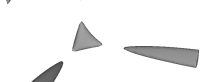
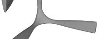
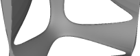
Figure 4: $\alpha$-suboptimal neighborhoods for the three-dimensional decomposed dynamics system with minimal coupling ($A=U=V^{\top}=I_{3\times 3}$) and breadth $\theta=100$. Neighborhoods shown for $\alpha$ ranging from $1.04$ to $1.2$ with a fixed controller.

5 Related work

Suboptimal coverings are closely related to several topics in control theory. Robust control synthesis under parametric uncertainty (Dullerud and Paganini, 2000) can be interpreted as seeking a policy that performs well on all of $\Phi$ without observing the particular ${\phi\in\Phi}$. Most problem statements in robust synthesis admit problem instances with no solution; the goal is to find a robust policy if one exists. Adaptive control is also concerned with sets of control tasks, with the added complication that $\phi$ is not known to the policy. Adaptive policies of the self-tuning type synthesize a single-task policy after estimating $\phi$, but this relies on the assumption that control synthesis can be computed quickly (Åström and Wittenmark, 2013).

Adaptive and gain-scheduled multi-model methods use a precomputed set of policies instead (Murray-Smith and Johansen, 1997), but researchers have focused more on the switching rule than the policy set. For example, Fu and Barmish (1986); Stilwell and Rugh (1999); Yoon et al. (2007) non-constructively assert the existence of a finite cover by continuity and compactness arguments. To address the need for small covers, Anderson et al. (2000); McNichols and Fadali (2003); Tan et al. (2004); Fekri et al. (2006); Du et al. (2012) propose constructive algorithms, sometimes with arguments for minimality, but without size bounds on the cover. Jalali and Golmohammad (2012) show an upper bound in terms of frequency-domain properties of $\Phi$, as opposed to state-space parameters like mass and geometry. The most closely related work to ours is from Fu (1996), who shows a tight bound of $2^{n}$ for the stability covering number of a relatively broad $\Phi$. This result is complementary to ours: suboptimality is a stronger criterion than stability, but our class of $\Phi$ is more restrictive. We are not aware of prior work that bounds covering numbers in a setup based on local suboptimality, as opposed to a single global performance measure.

Multi-task control is also a popular topic in deep learning research, where it is often motivated by ideas of lifelong skill acquisition in robotics. Domain randomization methods follow the spirit of robust control (Peng et al., 2017), but usually optimize for the average case instead of a worst-case guarantee. Many methods where the policy observes $\phi$ use architectural constructs that can only be applied to finite task sets (Yang et al., 2017; Parisotto et al., 2016; Devin et al., 2017). A common approach for infinite task spaces is to treat $\phi$ as a vector input alongside the system state. Yu et al. (2017); Chen et al. (2018) use this approach for dynamics parameters; Schaul et al. (2015) use it for navigation goals. There is evidence that policy class influences these methods: in a recent benchmark (Yu et al., 2019), the concatenated-input architecture trails the finite-task architecture. Other investigations into the difficulty of learning policies for multi-task control include methods to condition the multi-task optimization landscape (Yu et al., 2020) or balance disparate cost ranges (van Hasselt et al., 2016).

6 Conclusion and future work

In this paper, we introduced and motivated the $\alpha$-suboptimal covering number to quantify infinite task spaces for multi-task control problems. We defined a particular class of multi-task linear-quadratic regulator problems amenable to analysis of the $\alpha$-suboptimal covering number, and showed logarithmic dependency on the problem “breadth” parameter $\theta$ in the scalar case. Towards analogous results for the matrix case, we presented empirical studies intended to shed light on possible proof techniques. For the upper bound, we considered a natural covering construction that would preserve logarithmic dependence on $\theta$ but give exponential dependence on dimensionality. Experiments did not rule out its validity. For the lower bound, we visualized suboptimal neighborhoods for two possible system classes and observed interesting topological behavior for the minimal-coupling class.

After extending our current results to the matrix case, in future work the analysis can be applied to other classes of multi-task LQR problems including variations in $A,Q,R$, discrete time, and stochastic dynamics. It will be interesting to see if there are major differences between LQR variants. We also hope that suboptimal covers and covering numbers will be a useful tool for analyzing how the size of the task space affects the required expressiveness of function classes used in practice as multi-task policies, such as neural networks.

Appendix A Extended theoretical results

This appendix contains the proof for lem:subopt-convex. We first present some supporting material.

A.1 Supporting material

We begin by recalling the definition and properties of quasiconvex functions on $\mathbb{R}$. We then recall some basic facts about scalar LQR.

Definition A.1.

A function $f:\mathcal{D}\mapsto\mathbb{R}\$ on the convex domain $\ \mathcal{D}\subseteq\mathbb{R}^{n}$ is quasiconvex if its sublevel sets $\mathcal{D}_{\alpha}=\{x\in\mathcal{D}:f(x)\leq\alpha\}$ are convex for all $\alpha\in\mathbb{R}$.

Lemma A.2 (Boyd and Vandenberghe (2004), §3.4).

The following facts hold for quasiconvex functions on a convex $\mathcal{D}\subseteq\mathbb{R}$:

1. If $f:\mathbb{R}\mapsto\mathbb{R}$ is continuous, then $f$ is quasiconvex if and only if at least one of the following conditions holds on $\mathcal{D}$:

   1. $f$ is nondecreasing.

   2. $f$ is nonincreasing.

   3. There exists $c\in\mathcal{D}$ such that for all $t\in\mathcal{D}$, if $t<c$ then $f$ is nonincreasing, and if $t\geq c$ then $f$ is nondecreasing.

2. If $f:\mathbb{R}\mapsto\mathbb{R}$ is twice differentiable and $\partial^{2}f/\partial x^{2}>0$ for all $x\in\mathcal{D}$ where $\partial f/\partial x=0$, then $f$ is quasiconvex on $\mathcal{D}$.

3. If $f(x)=p(x)/q(x)$, where $p:\mathbb{R}\mapsto\mathbb{R}$ is convex with $p(x)\geq 0$ on $\mathcal{D}$ and $q:\mathbb{R}\mapsto\mathbb{R}$ is concave with $q(x)>0$ on $\mathcal{D}$, then $f$ is quasiconvex on $\mathcal{D}$.

The following facts about scalar LQR problems can be derived from the LQR Riccati equation and some calculus (not shown).

Lemma A.3.

For the scalar LQR problem with $a>0,b>0$ and $q=r=1$, the optimal linear controller $k^{\star}_{a,b}$ is given by the closed-form expression

$$k^{\star}_{a,b}=\min_{k\in\mathbb{R}}J_{a,b}(k)=\min_{k\in\mathbb{R}}\frac{1+k^{2}}{-2(a+bk)}=-\frac{a+\sqrt{a^{2}+b^{2}}}{b}.$$

For fixed $a$, the map from $b$ to $k^{\star}_{a,b}$ is continuous and strictly increasing on the domain $b\in(0,\infty)$ and has the range $(-\infty,-1)$. For any $k\in(-\infty,-1)$, there exists a unique $b_{k}\in(-\infty,-1)$ for which $k=k^{\star}_{a,b_{k}}$, given by

$$b_{k}=\frac{2ak}{1-k^{2}}.$$

A.2 Proof of lem:subopt-convex

We first recall the statement of the lemma. See 3.13

Instead of a monolithic proof, we present supporting material in lem:ratio-quasi,lem:cost-quasi. We then show the main result in lem:increasing-main, which considers $\alpha$-suboptimal neighborhoods on all of $\mathbb{R}$ instead of restricted to $\mathbf{B}$. lem:subopt-convex will follow as a corollary.

We proceed with more setup. Recall that the scalar DDF problem is defined by $\mathbf{A}=\{a\}$ and $\mathbf{B}=[\frac{1}{\theta},1]$, where $a>0$. For this section, let

$$\mathcal{D}=\{(b,k)\in(0,\infty)\times\mathbb{R}:a+bk<0\}$$

(note that $J_{b}(k)<\infty\iff a+bk<0$). Denote its projections by $\mathcal{D}^{b}(k)=\{b:(b,k)\in\mathcal{D}\}$ and $\mathcal{D}^{k}(b)=\{k:(b,k)\in\mathcal{D}\}$. We compute the suboptimality ratio $r:\mathcal{D}\mapsto\mathbb{R}$ by

$$r(b,k)=\frac{J_{b}(k)}{J^{\star}_{b}}=\left.\frac{1+k^{2}}{-2(a+bk)}\middle/\frac{a+\sqrt{a^{2}+b^{2}}}{b^{2}}\right.=\frac{(1+k^{2})b^{2}}{-2(a+bk)(a+\sqrt{a^{2}+b^{2}})}.$$

We denote its sublevel sets with respect to $b$ for fixed $k$ by

$$\mathcal{D}^{b}_{\alpha}(k)=\{b\in\mathcal{D}^{b}(k):r(b,k)\leq\alpha\}.$$

Lemma A.4.

For fixed $k<0$, the ratio $r(b,k)$ is quasiconvex on $\mathcal{D}^{b}_{k}$, and there is at most one $b\in\mathcal{D}^{b}_{k}$ at which $\partial r/\partial b=0$.

Proof A.5.

By inspection, $r(b,k)$ is smooth on $\mathcal{D}^{b}$. We now show that the second-order condition of lem:quasiconvex(b) holds. To solve $\partial r/\partial b=0$ for $b$, we multiply $\partial r/\partial b$ (not shown due to length) by the strictly positive factor

$$\frac{2\left(a+bk\right)^{2}\left(a+\sqrt{a^{2}+b^{2}}\right)^{2}\sqrt{a^{2}+b^{2}}}{ab\left(k^{2}+1\right)}$$

and set the result equal to zero to get the equation

$$2a^{2}+abk+b^{2}=\left(-2a-bk\right)\sqrt{a^{2}+b^{2}}.$$

Squaring both sides (which may introduce spurious solutions) and collecting terms yields the equation $-2ak-bk^{2}+b=0,$ with the solution $b={}$ $\frac{2ak}{1-k^{2}}$. This is the expression for $b_{k}$ from lem:scalar-lqr-facts. Note that it is only positive for $k<-1$. If $k\in[-1,0)$, then there are no stationary points in $\mathcal{D}^{b}_{k}$. Otherwise, substitution into $\partial r/\partial b$ confirms that this solution is not spurious, so it is the only stationary point of $r$ with respect to $b$. We now must check the second-order condition for $k<-1$. Evaluating $\partial^{2}r/\partial b^{2}$ (not shown due to length) and multiplying by the strictly positive factor

$$-\frac{\left(a+\sqrt{a^{2}+b^{2}}\right)\left(2a+2bk\right)}{k^{2}+1},$$

we have

$$\operatorname{sign}\left(\frac{\partial^{2}r}{\partial b^{2}}\right)=\operatorname{sign}\left(\frac{b^{4}}{\left(a+\sqrt{a^{2}+b^{2}}\right)\left(a^{2}+b^{2}\right)^{\frac{3}{2}}}+\frac{2b^{4}}{\left(a+\sqrt{a^{2}+b^{2}}\right)^{2}\left(a^{2}+b^{2}\right)}+\frac{2b^{3}k}{\left(a+bk\right)\left(a+\sqrt{a^{2}+b^{2}}\right)\sqrt{a^{2}+b^{2}}}+\frac{2b^{2}k^{2}}{\left(a+bk\right)^{2}}-\frac{5b^{2}}{\left(a+\sqrt{a^{2}+b^{2}}\right)\sqrt{a^{2}+b^{2}}}-\frac{4bk}{a+bk}+2\right).$$

Evaluating at the stationary point $b_{k}$, this reduces to

$$\left.\operatorname{sign}\left(\frac{\partial^{2}r}{\partial b^{2}}\right)\right|_{b_{k},k}=\operatorname{sign}\left(\frac{2k^{2}\left(k-1\right)^{2}\left(k+1\right)^{2}}{\left(k^{2}+1\right)^{3}}\right).$$

Recalling that $k<-1$, the sign is positive. The conclusion follows from lem:quasiconvex(b).

Lemma A.6.

For fixed $b$, the cost $J_{b}(k)$ is quasiconvex on $\mathcal{D}^{k}(b)$. Also, $J_{b}(k)$ is not monotonic, so case (a)3. of lem:quasiconvex(a) applies.

Proof A.7.

We have

$$J_{b}(k)=\frac{1+k^{2}}{-2(a+bk)}.$$

The numerator is nonnegative and convex on $k\in\mathbb{R}$. The denominator is linear (hence concave) and positive on $\mathcal{D}^{k}(b)$. Quasiconvexity follows from lem:quasiconvex(c). Nonmonotonicity follows from the fact that $J_{b}(k)$ is smooth on $\mathcal{D}^{k}(b)$ and has a unique optimum at $k^{\star}_{b}$, which is not on the boundary of $\mathcal{D}^{k}(b)$.

We now combine these into the main result.

Lemma A.8.

For a scalar DDF problem, if $\alpha>1$ and $k<-1$, then $\mathcal{D}^{b}_{\alpha}(k)$ is either: a bounded closed interval $[b_{1},b_{2}]$, with $b_{1}$ and $b_{2}$ increasing in $k$, or a half-bounded closed interval $[b_{1},\infty)$, with $b_{1}$ increasing in $k$.

Proof A.9.

By lem:ratio-quasi, due to quasiconvexity $\mathcal{D}^{b}_{\alpha}$ is convex. The only convex sets on $\mathbb{R}$ are the empty set and all types of intervals: open, closed, and half-open. We know $\mathcal{D}^{b}_{\alpha}$ is not empty because it contains $b_{k}$. We can further assert that $\mathcal{D}^{b}_{\alpha}$ has a closed lower bound because $\lim_{b\to(-a/k)}r(b,k)=\infty$ (see Boyd and Vandenberghe (2004, §A.3.3) for details). However, the upper bound may be closed or infinite. We handle the two cases separately.

Bounded case.

Fix $k_{0}<-1$. Suppose $\mathcal{D}^{b}_{\alpha}(k_{0})=[b_{1},b_{2}]$ for $0<b_{1}<b_{2}<\infty$. By the implicit function theorem (IFT), at any $(b_{0},k_{0})$ satisfying $r(b_{0},k_{0})=\alpha$, if $\partial r/\partial b|_{b_{0},k_{0}}\neq 0$ then there exists an open neighborhood around $(b_{0},k_{0})$ for which the solution to $r(b,k)=\alpha$ can be expressed as $(g(k),k)$, where $g$ is a continuous function of $k$ and

$$\left.\frac{\partial g(k)}{\partial k}\right|_{k_{0}}=\left.-\left(\frac{\partial r}{\partial b}\right)^{-1}\frac{\partial r}{\partial k}\right|_{b_{0},k_{0}}.$$

By the continuity and quasiconvexity of $r$, and the fact that $\partial r/\partial b=0$ only at $b_{k}$ (lem:ratio-quasi) we know that $r(b_{1},k_{0})=r(b_{2},k_{0})=\alpha$ and

$$\left.\frac{\partial r}{\partial b}\right|_{b_{1},k_{0}}<0\quad\text{and}\quad\left.\frac{\partial r}{\partial b}\right|_{b_{2},k_{0}}>0.$$

By lem:scalar-lqr-facts, since $k<-1$ there exists $b_{k}>0$ satisfying $k=k^{\star}_{b_{k}}$. Since $r(b_{k},k)=1$ and $\alpha>1$, we know $b_{k_{0}}\in(b_{1},b_{2})$. Again by lem:scalar-lqr-facts, the map from $b$ to $k^{\star}_{b}$ is increasing in $b$. Therefore, ${k^{\star}_{b_{1}}<k_{0}<k^{\star}_{b_{2}}}.$ By the quasiconvexity and nonmonotonicity of $J_{b}(k)$ from lem:cost-quasi, via lem:quasiconvex(a) we have

$$\left.\frac{\partial r}{\partial k}\right|_{b_{1},k_{0}}\geq 0\quad\text{and}\quad\left.\frac{\partial r}{\partial k}\right|_{b_{2},k_{0}}\leq 0.$$

Therefore, the functions $g_{1},g_{2}$ satisfying the conclusion of the IFT in the neighborhoods around $(b_{1},k_{0})$ and $(b_{2},k_{0})$ respectively also satisfy

$$\left.\frac{\partial g_{1}(k)}{\partial k}\right|_{b_{1},k_{0}}\geq 0\quad\text{and}\quad\left.\frac{\partial g_{2}(k)}{\partial k}\right|_{b_{2},k_{0}}\geq 0.$$

Therefore, $b_{1}$ and $b_{2}$ are locally nondecreasing in $k$.

Unbounded case.

Suppose $\mathcal{D}^{b}_{\alpha}(k)=[b_{1},\infty)$ for $b_{1}<\infty$. By the same IFT argument as in the bounded case, $b_{1}$ is increasing in $k$. By the quasiconvexity of $r$ in $b$, the value of $r$ is increasing for $b>b_{k}$, but the definition of $\mathcal{D}^{b}_{\alpha}(k)$ implies that $r(b,k)\leq\alpha$ for all $b>b_{k}$. Therefore, $\lim_{b\to\infty}r(b,k)$ exists and is bounded by $\alpha$. In particular,

$$\begin{split}\lim_{b\to\infty}r(b,k)&=\lim_{b\to\infty}\frac{(1+k^{2})b^{2}}{-2(a+bk)(a+\sqrt{a^{2}+b^{2}})}\\ &=\lim_{b\to\infty}\frac{(1+k^{2})b^{2}/b^{2}}{-2(a+bk)(a+\sqrt{a^{2}+b^{2}})/b^{2}}\\ &=-\frac{1+k^{2}}{2k}.\end{split}$$

Taking the derivative shows that this value is decreasing in $k$ for $k<0$. Therefore, if $k<k^{\prime}<0$ then

$$\lim_{b\to\infty}r(b,k^{\prime})\leq\lim_{b\to\infty}r(b,k)\leq\alpha.$$

The property that $r(b,k^{\prime})$ is increasing in $b$ for $b>b_{k}$ further ensures that $r(b,k^{\prime})\leq\alpha$ for all $b>b_{k}$. Therefore, $\mathcal{D}^{b}_{\alpha}(k^{\prime})$ is also unbounded.

For completeness, we prove lem:subopt-convex.

Proof A.10.

(of lem:subopt-convex). By lem:increasing-main, $\mathcal{D}^{b}_{\alpha}(k)$ is either a bounded closed interval $[b_{1},b_{2}]$, with $b_{1}$ and $b_{2}$ increasing in $k$, or a half-bounded closed interval $[b_{1},\infty)$, with $b_{1}$ increasing in $k$. Recall that $\mathscr{N}_{\alpha}(k)=\mathcal{D}^{b}_{\alpha}(k)\cap\mathbf{B}$ with $\mathbf{B}=[\frac{1}{\theta},1]$. Therefore, the half-bounded case can be reduced to the bounded case with $b_{2}=1$. The intersection can be expressed as

$$\mathscr{N}_{\alpha}(k)=[\max\{b_{1},\textstyle\frac{1}{\theta}\},\min\{b_{2},1\}],$$

where the interval $[a,b]$ is defined as the empty set if $a>b$. Taking the maximum or minimum of a nonstrict monotonic function and a constant preserves the monotonicity, so we are done.

References

- Anderson et al. (2000) Brian D. O. Anderson, Thomas S. Brinsmead, Franky De Bruyne, Joao Hespanha, Daniel Liberzon, and A. Stephen Morse. Multiple model adaptive control. part 1: Finite controller coverings. International Journal of Robust and Nonlinear Control, 10(11-12):909–929, 2000.
- Åström and Wittenmark (2013) Karl J Åström and Björn Wittenmark. Adaptive Control. Courier Corporation, 2013.
- Boyd and Vandenberghe (2004) Stephen Boyd and Lieven Vandenberghe. Convex Optimization. Cambridge University Press, 2004.
- Bu et al. (2019) Jingjing Bu, Afshin Mesbahi, and Mehran Mesbahi. On topological and metrical properties of stabilizing feedback gains: the MIMO case. CoRR, abs/1904.02737, 2019.
- Chen et al. (2018) Tao Chen, Adithyavairavan Murali, and Abhinav Gupta. Hardware conditioned policies for multi-robot transfer learning. In NeurIPS, pages 9355–9366, 2018.
- Devin et al. (2017) Coline Devin, Abhishek Gupta, Trevor Darrell, Pieter Abbeel, and Sergey Levine. Learning modular neural network policies for multi-task and multi-robot transfer. In IEEE International Conference on Robotics and Automation (ICRA), pages 2169–2176, 2017.
- Du et al. (2012) Jingjing Du, Chunyue Song, and Ping Li. Multimodel control of nonlinear systems: An integrated design procedure based on gap metric and loop shaping. Industrial & Engineering Chemistry Research, 51(9):3722–3731, 2012.
- Dullerud and Paganini (2000) Geir E. Dullerud and Fernando Paganini. A Course in Robust Control Theory: A Convex Approach. Springer-Verlag New York, 2000.
- Fazel et al. (2018) Maryam Fazel, Rong Ge, Sham M. Kakade, and Mehran Mesbahi. Global convergence of policy gradient methods for linearized control problems. CoRR, abs/1801.05039, 2018.
- Fekri et al. (2006) Sajjad Fekri, Michael Athans, and Antonio Pascoal. Issues, progress and new results in robust adaptive control. International Journal of Adaptive Control and Signal Processing, 20(10):519–579, 2006.
- Fu (1996) Minyue Fu. Minimum switching control for adaptive tracking. In Proceedings of 35th IEEE Conference on Decision and Control, volume 4, pages 3749–3754, 1996.
- Fu and Barmish (1986) Minyue Fu and B. Ross Barmish. Adaptive stabilization of linear systems via switching control. IEEE Transactions on Automatic Control, 31(12):1097–1103, 1986.
- Jalali and Golmohammad (2012) Ali Akbar Jalali and Hassan Golmohammad. An optimal multiple-model strategy to design a controller for nonlinear processes: A boiler-turbine unit. Computers & Chemical Engineering, 46:48–58, 2012.
- Kalman (1960) R. E. Kalman. Contributions to the theory of optimal control. Boletín de la Sociedad Matemática Mexicana, 5:102–199, 1960.
- Lancaster and Rodman (1995) Peter Lancaster and Leiba Rodman. Algebraic Riccati Equations. Clarendon Press, 1995.
- McNichols and Fadali (2003) Kenneth H. McNichols and M. Sami Fadali. Selecting operating points for discrete-time gain scheduling. Computers & Electrical Engineering, 29(2):289–301, 2003.
- Murray-Smith and Johansen (1997) Roderick Murray-Smith and Tor Arne Johansen. Multiple Model Approaches to Modelling and Control. Taylor and Francis, London, 1997.
- Parisotto et al. (2016) Emilio Parisotto, Lei Jimmy Ba, and Ruslan Salakhutdinov. Actor-mimic: Deep multitask and transfer reinforcement learning. In International Conference on Learning Representations (ICLR), 2016.
- Peng et al. (2017) Xue Bin Peng, Marcin Andrychowicz, Wojciech Zaremba, and Pieter Abbeel. Sim-to-real transfer of robotic control with dynamics randomization. CoRR, abs/1710.06537, 2017.
- Petersen and McFarlane (1994) Ian R. Petersen and Duncan C. McFarlane. Optimal guaranteed cost control and filtering for uncertain linear systems. IEEE Transactions on Automatic Control, 39(9):1971–1977, 1994.
- Schaul et al. (2015) Tom Schaul, Daniel Horgan, Karol Gregor, and David Silver. Universal value function approximators. volume 37 of Proceedings of Machine Learning Research, pages 1312–1320, Lille, France, Jul 2015.
- Stilwell and Rugh (1999) Daniel J. Stilwell and Wilson J. Rugh. Interpolation of observer state feedback controllers for gain scheduling. IEEE Transactions on Automatic Control, 44(6):1225–1229, 1999.
- Tan et al. (2004) Wen Tan, Horacio J. Marquez, and Tongwen Chen. Operating point selection in multimodel controller design. In Proceedings of the 2004 American Control Conference, volume 4, pages 3652–3657, 2004.
- van Hasselt et al. (2016) Hado P van Hasselt, Arthur Guez, Matteo Hessel, Volodymyr Mnih, and David Silver. Learning values across many orders of magnitude. In Advances in Neural Information Processing Systems, pages 4287–4295, 2016.
- Yang et al. (2017) Zhaoyang Yang, Kathryn E Merrick, Hussein A Abbass, and Lianwen Jin. Multi-task deep reinforcement learning for continuous action control. In IJCAI, pages 3301–3307, 2017.
- Yoon et al. (2007) Myung-Gon Yoon, Valery A. Ugrinovskii, and Marek Pszczel. Gain-scheduling of minimax optimal state-feedback controllers for uncertain LPV systems. IEEE Transactions on Automatic Control, 52(2):311–317, 2007.
- Yu et al. (2019) Tianhe Yu, Deirdre Quillen, Zhanpeng He, Ryan Julian, Karol Hausman, Chelsea Finn, and Sergey Levine. Meta-world: A benchmark and evaluation for multi-task and meta reinforcement learning. In CoRL, volume 100 of Proceedings of Machine Learning Research, pages 1094–1100. PMLR, 2019.
- Yu et al. (2020) Tianhe Yu, Saurabh Kumar, Abhishek Gupta, Sergey Levine, Karol Hausman, and Chelsea Finn. Gradient surgery for multi-task learning. CoRR, abs/2001.06782, 2020.
- Yu et al. (2017) Wenhao Yu, Jie Tan, C. Karen Liu, and Greg Turk. Preparing for the unknown: Learning a universal policy with online system identification. In Robotics: Science and Systems (RSS), 2017.