One-Round Active Learning

Abstract

In this work, we initiate the study of one-round active learning, which aims to select a subset of unlabeled data points that achieve the highest model performance after being labeled with only the information from initially labeled data points. The challenge of directly applying existing data selection criteria to the one-round setting is that they are not indicative of model performance when available labeled data is limited. We address the challenge by explicitly modeling the dependence of model performance on the dataset. Specifically, we propose DULO, a data-driven framework for one-round active learning, wherein we learn a model to predict the model performance for a given dataset and then leverage this model to guide the selection of unlabeled data. Our results demonstrate that DULO leads to the state-of-the-art performance on various active learning benchmarks in the one-round setting.

Introduction

The success of deep learning largely depends on the access to large labeled datasets; yet, annotating a large dataset is often costly and time-consuming. Active learning (AL) has been the main solution to reducing labeling costs. The goal of AL is to select the most informative points from unlabeled data set to be labeled, so that the accuracy of the classifier increases quickly as the set of labeled examples grows. AL (Fine, Gilad-Bachrach, and Shamir 2002; Freund et al. 1997; Graepel and Herbrich 2000; Seung, Opper, and Sompolinsky 1992; Campbell et al. 2000; Schohn and Cohn 2000; Tong and Koller 2001) typically works in multiple rounds, where each round builds a classifier based on the current training set, and then selects the next example to be labeled. This procedure is repeated until we reach a good model or exceeds the labeling budget.

The multi-round nature of the existing AL framework poses great challenges to its wide adaption. Firstly, there lacks specialized platforms where annotators can interact online with the data owner and provide timely feedback. For instance, the existing broadly used data labeling approaches, such as crowdsourcing (e.g., Amazon Mechanical Turk) and outsourcing to companies, do not support a timely interaction between the data owner and annotators. Second, even if one can find such interactive annotators, it is often inefficient to acquire labels one-by-one, especially when each label takes substantial time or when the training process is time-consuming. Various batch-mode AL algorithms (Hoi et al. 2006; Sener and Savarese 2017; Ash et al. 2019a; Kirsch, Van Amersfoort, and Gal 2019; Wei, Iyer, and Bilmes 2015; Killamsetty et al. 2020) have been proposed to improve labeling efficiency by selecting multiple examples to be labeled in each round. However, for these algorithms to be effective, they still require many rounds of interaction. Since the examples selected in the current round depend on the examples selected in all previous rounds, existing batch AL algorithms cannot make full advantage of parallel labeling.

In light of the aforementioned challenges of multi-round AL, we initiate the study of one-round AL, where only one round of data selection and label query is allowed. One-round AL starts with very few labeled data points (e.g. a small amount of randomly selected data that are labeled internally or externally). By exploiting these initially labeled data points, a one-round AL strategy selects a large subset of unlabeled data points that could potentially achieve high data utility after being labeled, and then queries their labels all at once. Importantly, in the one-round setting, the selected data points can be labeled completely in parallel.

A straightforward approach to one-round AL is to directly use the data selection criteria from the existing multi-round AL methods to perform one-round selection. However, these criteria cannot reliably select unlabeled points resulting in high model performance in one-round setting where only limited labeled data is available. Some of the existing criteria are calculated based on individual predictions of the model trained on the available labeled data (Wei, Iyer, and Bilmes 2015; Ash et al. 2019b; Wei, Iyer, and Bilmes 2015; Killamsetty et al. 2020), which tend to be erroneous with very limited labeled data. Others rely on heuristics (e.g., uncertainty (Lewis and Gale 1994) and diversity (Seung, Opper, and Sompolinsky 1992; Sener and Savarese 2017)) that are only weakly correlated with the model performance; worse yet, these heuristics are also calculated from the model trained on the available labeled data, thus becoming even less effective when labeled data points are very limited.

In this paper, we propose a general one-round AL framework via Data Utility function Learning and Optimization (DULO). Our framework is grounded on the notion of data utility functions, which map any given set of unlabeled data points to some performance measure of the model trained on the set after being labeled. We propose a natural formulation of the one-round AL problem, which is to seek the set of unlabeled points maximizing the data utility function. We adopt a sampled-based approach to learn a parametric model that approximates the data utility function, and then leverage greedy algorithms to optimize the learned model. We further propose several strategies to improve scalability. Specifically, to improve efficiency for learning the data utility function for a large model, we propose to learn it based on a simple proxy model instead of the original model; to improve efficiency for optimizing the data utility function for large unlabeled data, we propose to perform greedy optimization over a block of unlabeled data instead of the entire set.

Our contributions can be summarized as follows. (1) We present the first focused study of one-round AL, an important yet underexplored setting, and develop an algorithm based on data utility function learning and optimization. (2) We exhibit several novel empirical observations about data utility functions, including approximate submodularity and their transferrability between different learning algorithms, which provide actionable insights into boosting the efficiency of data utility learning and optimization. (3) We perform extensive experiments and show that DULO compares favorably to performing state-of-art batch AL algorithms for one round—a natural baseline for one-round AL—on different datasets and models.

Related Work

Earlier studies of AL focused on the setting where only one example is selected in each round (Fine, Gilad-Bachrach, and Shamir 2002; Freund et al. 1997; Graepel and Herbrich 2000; Seung, Opper, and Sompolinsky 1992; Campbell et al. 2000; Schohn and Cohn 2000; Tong and Koller 2001). These methods could be time-consuming as they require many rounds of interaction with the data labeler. Batch AL (Hoi et al. 2006) was later proposed to improve the efficiency of label acquisition by querying multiple examples in each round. However, their selection strategy fails to capture the diversity of examples in a batch, thereby often ending up picking redundant examples. Recent works on batch AL have attempted to enhance the diversity of a batch. For instance, core-set (Sener and Savarese 2017) uses $k$-center clustering to select informative data points while preserving the geometry of data points. However, it only works well for simple datasets or for models with good architectural prior. More recently, BADGE (Ash et al. 2019a) proposes to sample a batch of data points whose gradients have high magnitude and diverse directions. This method relies on partially-trained models to acquire hypothesized labels and further rank unlabeled data points for selection.

Existing batch AL methods have utilized submodular acquisition function to enable efficient selection over large unlabeled datasets (Wei, Iyer, and Bilmes 2014; Buchbinder et al. 2014; Bairi et al. 2015; Wei et al. 2014; Wei, Iyer, and Bilmes 2015; Killamsetty et al. 2020). However, the submodular acquisition functions in the existing literature usually rely on hypothesized labels assigned by the partially-trained classifier. For instance, one popular approach, Filtered Active Submodular Selection (FASS) (Wei, Iyer, and Bilmes 2015), selects unlabeled data points by optimizing the data utility functions of simple classifiers such as KNN or Naive Bayes. The data utility functions for these simple models have analytical form and are proven to be submodular under certain assumptions. These submodular utility functions require label information as input, so in order to optimize the submodular acquisition functions over the unlabeled data pool, we need to assign each unlabeled data point with hypothesized label using the partially-trained classifier. This can lead to poor selection performance at the initial few rounds as the classifiers’ accuracy is usually low at the beginning. Another related state-of-art approach (Killamsetty et al. 2020) performs data selection and model training alternatively using these simple classifiers’ submodular utility function and shares the same limitation as FASS and BADGE due to the use of hypothesized labels. In contrast, our acquisition functions directly estimate the utility of an unlabeled dataset and thus do not require hypothesized labels.

While recent work on batch AL shows promising results for choosing high-quality data with multi-round selection, our experiments show that with one round, even the state-of-the-art techniques cannot attain satisfactory performance.

Data Utility Functions

Formalization

A data utility function is a mapping from a set of unlabeled data points to a real number indicating the utility of the set. The metrics for utility could be context-dependent. For instance, in AL, the typical goal is to select a set of unlabeled points that can lead to a classifier with the highest test accuracy after labeling. Hence, a natural choice for data utility is the test accuracy of the classifier trained on the selected unlabeled dataset and their corresponding labels.

More formally, we define data utility function in terms of the notion of learning algorithm and metric function. Let $S_{x}=\{x_{i}\}_{i=1}^{n}$ denote a set of features and $f^{*}$ be the ground-truth function that produce the label for any given feature input. A learning algorithm $\mathcal{A}$ is a function that takes a training set $S=\{(x_{i},f^{*}(x_{i}))\}_{i=1}^{n}$ and returns a classifier $f$ which approximates $f^{*}$. A metric function $u$ takes a classifier as input and outputs its model utility. If we define model utility as test accuracy, the metric function is defined as $u(f,\mathcal{V})=\frac{1}{|\mathcal{V}|}\sum_{(x,f^{*}(x))\in\mathcal{V}}\mathbbm{1}[f(x)=f^{*}(x)]$ for a test set $\mathcal{V}$ drawn from the same distribution as the training set. However, test set $\mathcal{V}$ is usually not available during the training time. In practice, $u(f,\mathcal{V})$ is typically approximated by validation accuracy $u(f,V)$ where $V$ is a validation set separated from the training set. With a learning algorithm $\mathcal{A}$, a corresponding metric function $u$ and the ground-truth function $f^{*}$, we define the data utility function as $U_{\mathcal{A},u,f^{*}}(S_{x})=u(\mathcal{A}((S_{x},f^{*}(S_{x}))),\mathcal{V})$, where we slightly abuse the notation and use $f^{*}(S_{x})$ to denote the set of labels $\{f^{*}(x)\}_{x\in S_{x}}$.

Approximate Submodularity

With the notion of data utility functions, one can formulate an AL problem as an optimization problem that seeks the set of unlabeled data points maximizing the data utility function. However, each evaluation of data utility function requires retraining the model on the input dataset. Thus, we propose to train a parametric model (dubbed a data utility model hereinafter) to approximate data utility functions. The AL task will then becomes optimizing the data utility model over the unlabeled data pool. However, the data utility function is a set function; a general set function is not efficiently learnable (Balcan and Harvey 2011) and at the same time, optimizing a general set function is NP-hard (Feige 1998).

Fortunately, our empirical studies show that data utility functions exhibit “approximate” submodularity. Submodular functions are almost always being characterized by the “diminishing return” property. Formally, a set function $f:2^{V}\rightarrow\mathbb{R}$ returning a real value for any subset $S\subseteq V$ is submodular if $f(\{j\}\cup S)-f(S)\geq f(\{j\}\cup T)-f(T),\forall S\subseteq T,j\in V\setminus T$. Figure 1 shows some examples of the marginal contributions of a fixed data point versus the sizes of a sequence of data subsets. A clear “diminishing returns” phenomenon can be observed from the figure, in which an extra training data point contributes less to model accuracy as the base training set size increases. Moreover, this phenomenon is observed on almost every common ML algorithm we test, including complicated models like deep neural networks. Due to space constraint, we defer more examples of such marginal contribution plots on different datasets and models into the Appendix.

The framework proposed in this paper is greatly inspired by this empirical observation, because it is known that submodular functions can be learned and optimized efficiently. Specifically, it has been theoretically shown that (approximate) submodular functions are PMAC/PAC-learnable with polynomially many independent samples (Balcan and Harvey 2011; Feldman and Vondrák 2016; Feldman, Kothari, and Vondrák 2020; Wang, Yang, and Jia 2021). Moreover, (approximate) submodular functions can be optimized efficiently by simple greedy algorithms (Minoux 1978; Horel and Singer 2016; Hassidim and Singer 2018).

As a final note, although different learning algorithms’ data utility functions consistently exhibit approximate submodularity, the rigorous proof is surprisingly hard. Exact submodularity has thus far been proved for only three simple classes of classifiers–Naive Bayes, Nearest Neighbors, and linear regression, under some strict assumptions (Wei, Iyer, and Bilmes 2015; Killamsetty et al. 2020). We leave the rigorous proof of the approximate submodularity for more widely used models such as logistic regression and deep nets as important future works.

Learning Data Utility Model with DeepSets

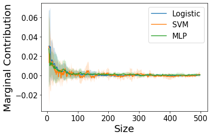
Figure 1: An illustration of “diminishing return” property of data utility functions for widely used learning algorithm (trained on USPS dataset, see specific settings in Appendix): given a training set $D$ of size $n$, we randomly sample a data point $j\in D$ at the beginning. We then start with an empty set $S_{0}=\emptyset$. For each $i\in\{1,\ldots,n\}$, we randomly sample a data point $k\in D/(S\cup\{j\})$ each time and obtain $S_{i}=S_{i-1}\cup\{k\}$. Therefore we have $S_{0}\subset S_{1}\subset\ldots S_{n}$. For each $S_{i}$, we record the marginal contribution of data point $j$, i.e., $U_{\mathcal{A},u}(S_{i}\cup\{j\})-U_{\mathcal{A},u}(S_{i})$. We repeat the above procedures for 10 different data point $j$ and plot the average of marginal contributions against the size of $S_{i}$. The procedure exactly matches the definition of submodularity.

Suppose that we have $N$ labeled samples $\mathcal{L}=\{(x_{i},f^{*}(x_{i}))\}_{i=1}^{N}$. To learn the data utility model, we first split $\mathcal{L}$ into training set $\mathcal{L}_{tr}$ and validation set $\mathcal{L}_{val}$, where $\mathcal{L}_{tr}$ is used for model training and $\mathcal{L}_{val}$ is used for evaluating the data utility. Specifically, we train a classifier $f$ on a subset $S\subseteq\mathcal{L}_{tr}$ and calculate the validation accuracy of $f$ on $\mathcal{L}_{val}$, which gives us $u(f,\mathcal{L}_{val})$. If we train the classifier $f$ for multiple times with different subsets $S$, the set $\{(S_{x},u(f,\mathcal{L}_{val}))\}$ could serve as a training set for learning $U_{\mathcal{A},u,f^{*}}$, where $S_{x}$ denote the set of features of $S$. We adopt a canonical model architecture for set function learning–DeepSets (Zaheer et al. 2017)–as our model for $U_{\mathcal{A},u,f^{*}}$. DeepSets is a permutation-invariant type of neural networks, making it suitable for modeling set-valued functions. We then train a DeepSets model $f_{DS}$ on $\{(S_{x},u(f,\mathcal{L}_{val}))\}$ to approximate $U_{\mathcal{A},u,f^{*}}$. Algorithm 1 summarizes our algorithm for training data utility model. For consistency, in the following text, we refer to $\mathcal{L}_{tr}$ as labeled training dataset, and $\mathcal{L}_{val}$ as labeled validation dataset.

input : $\mathcal{L}$ - initially labeled samples, $\mathcal{A}$ - training algorithm for classifier $f$, $u$ - metric function, $\mathcal{A}_{DS}$ - training algorithm for DeepSets model $f_{DS}$, $r$ - train-validation split ratio, $T$ - number of classifiers to be trained

output : $f_{DS}$ - DeepSets utility model which approximates $U_{\mathcal{A},u,f^{*}}$.

1

2Split $\mathcal{L}$ into training set $\mathcal{L}_{tr}$ and validation set $\mathcal{L}_{val}$ according to ratio $r$.

3Initialize training set for DeepSets utility model $S_{DS}=\emptyset$.

4for $t=1,\dots,T$ do

5       Randomly choose a subset $S=(S_{x},f^{*}(S_{x}))\subseteq\mathcal{L}_{tr}$.

6      Train classifier $f\leftarrow\mathcal{A}(S)$.

7      $S_{DS}=S_{DS}\cup\{(S_{x},u(f,\mathcal{L}_{val}))\}$.

8 end for

9

10Train $f_{DS}\leftarrow\mathcal{A}_{DS}(S_{DS})$.

return $f_{DS}$

Algorithm 1 DeepSets Data Utility Learning.

One-Round AL via DULO

Core Algorithm

The full algorithm for our proposed one-round AL approach, which we call DULO, is summarized in Algorithm 2. In a high level, the algorithm first learns the data utility function using the initial labeled dataset and then optimizes the trained data utility model to select the most useful unlabeled data points. The learned data utility model $f_{DS}$ predicts the test accuracy of the model trained on a given set of unlabeled data once they are correctly labeled. The unlabeled data selection problem can be formalized as follows:

$$\operatorname*{arg\,max}_{|S_{x}|=M,S_{x}\subseteq\mathcal{U}}f_{DS}(S_{x})$$ (1)

where $M$ is the labeling budget for the selected subset. Since most of the data utility functions are empirically shown to be approximately submodular, we could solve (1) efficiently and approximately using greedy algorithms. We choose to apply stochastic greedy optimization from Mirzasoleiman et al. (2015) to solve (1) because it runs in linear time while provides $1-1/e-\epsilon$ approximation guarantee.

Improving Scalability

The naive implementation of DULO is computationally impractical for large models. This is because constructing training samples for the data utility model requires retraining models for many times, which is very slow for large models. Besides, the clock-time of each DeepSets evaluation increases significantly when the input set sizes grows; hence, optimizing the data utility model over a large unlabeled data pool is expensive. Next, we present strategies to enable DULO to be scalable to large models and large unlabeled data size.

Scale to Large Models.

Constructing a size-$T$ training set for learning the data utility model requires retraining the classifier for $T$ times. In experiments, we found that for the data utility function to be learned accurately, we often need to train a classifier thousands of times. The computational costs incurred by this process are acceptable for logistic regression or small CNN models, because the initial labeled dataset is usually very small and it takes minimal time to train one model on it. In our experiment, training 1000 logistic regression models on 300 MNIST images in PyTorch (Paszke et al. 2019) only requires around 30 minutes with NVIDIA Tesla K80 GPU, and training 1000 small CNN models on 500 CIFAR-10 images just takes about 4 hours. Besides, since the training of these models is completely independent of each other, constructing training samples for data utility model could be accelerated through parallelization without any communication overhead.

However, for relatively large models such as GPT-3 (Brown et al. 2020) or very deep ResNets, training on a small dataset multiple times could still be extremely time- or memory-consuming. We resolve this problem by utilizing the transferrability of data utility from one learning algorithm to another—data points useful for one learning algorithm are usually useful for other learning algorithms. Such transferrability also leveraged in designing efficient data valuation algorithms (Jia et al. 2019). Figure 2 shows an example of such correlation between data utilities. As we can see, the logistic regression’s accuracies are positively correlated with the LeNet’s accuracies, although the LeNet performs much better than the logistic regression. More such examples are provided in the Appendix. Based on this observation, we propose to use a proxy model when training original models thousands of times on the initial labeled dataset exceeds time or memory budget. The proxy model should be small enough to be trained efficiently, while still achieving observable performance improvement after training. When there are too many classes and classification accuracy improvements are hardly noticeable, we can use less stringent utility metrics functions such as Top-5 accuracy.

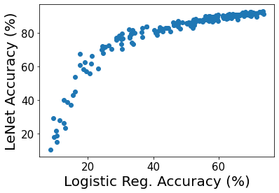
Figure 2: Example of the correlation between data utilities for different learning algorithms: for each point in the figure, we randomly sample 2000 MNIST data points, add Gaussian noise to a random portion of the images, and record the accuracies of logistic regression and LeNet trained on the selected samples. Spearman rank correlation here is 0.968.

Scale to Large Unlabeled Data Pool.

Another design choice of our one-round AL framework is to deal with the situation when the size of unlabeled dataset is much larger than the labeled set, i.e. $|\mathcal{U}|\gg|\mathcal{L}_{tr}|$. In this case, the generalizability of DeepSets models to giant input sets is questionable, because the largest possible data size that the DeepSets model has seen during training is $|\mathcal{L}_{tr}|$. Besides, evaluation time of DeepSets will significantly increase for larger input set sizes, which makes the linear-time stochastic greedy algorithm become inefficient in practice. We tackle this challenge by running greedy optimization with a subset $\mathcal{B}\subseteq\mathcal{U}$ of an appropriate size $B$. $B$ should be chosen such that the DeepSets data utility model has both good generalizability and efficient evaluation. We can repeat the above process for $\frac{|\mathcal{U}|}{B}$ times and each time, we select $\frac{MB}{|\mathcal{U}|}$ data points from each of $\mathcal{B}$. We call parameter $B$ as optimization block size in Algorithm 2. Although breaking down the selected data into different blocks, we want to highlight that this design is completely different from batch AL, since we do not require the data points selected in the previous blocks to be labeled before we select data points from the current block. Therefore, the WHILE loop in Algorithm 2 is fully parallelizable. One may concern that choosing data points independently from each block would fail to capture the interactions between the data selected from different blocks. However, as long as the optimization block size is reasonably large, the missed high-level interactions are negligible. We perform an ablation study for optimization block size $B$ in the Appendix.

input : ($\mathcal{L}$, $\mathcal{A}$, $\mathcal{A}_{DS}$, $u$, $r$, $T$) - same inputs as Algorithm 1, $\mathcal{U}$ - unlabeled samples, $M$ - labeling budget, $B$ - optimization block size, $\epsilon$ - precision parameter for stochastic greedy algorithm.

output : $S_{selected}$ - selected set.

11

12$f_{DS}\leftarrow\text{DeepSetsDataUtilityLearning}(\mathcal{L},\mathcal{A},\mathcal{A}_{DS},u,r,T)$

13Initialize $S_{selected}=\emptyset$.

14while  $|S_{selected}|<M$  do

15       Sample $\mathcal{B}\subseteq\mathcal{U}$ of size $B$.

16      $S_{x}\leftarrow\emptyset$

17      while  $|S_{x}|<\frac{MB}{|\mathcal{U}|}$  do

18             Sample $Z\subseteq\mathcal{B}\setminus S_{x}$ of size $\frac{|\mathcal{U}|}{M}\log(\frac{1}{\log\epsilon})$

19            Find $e=\operatorname*{arg\,max}_{e\in Z}f_{DS}(S_{x}\cup\{e\})$

20            $S_{x}\leftarrow S_{x}\cup\{e\}$

21       end while

22      

23      $S_{selected}=S_{selected}\cup S_{x}$.

24      $\mathcal{U}=\mathcal{U}\setminus S_{x}$.

25 end while

26

return $S_{selected}$

Algorithm 2 DULO for one-round AL with stochastic greedy optimization

Evaluation

Experimental Settings

Evaluation Protocols

We evaluate the performance of different AL strategies on different types of models and a varied amount of selected data points. Notably, we assess the performance of DULO for models that are more complicated than proxy model. For example, we use logistic regression as the proxy model for MNIST, while examine the utility of the selected data for LeNet. We evaluate the robustness of DULO on different practical scenarios such as imbalanced or noisy unlabeled datasets. We also test the performance on real-world datasets and provide insights into the selected data. Finally, we perform ablation studies for sample complexity, hyperparameters, and potential variant for DULO. Due to space constraint, we present the results for DULO’s sample complexity here and defer other results to Appendix.

Datasets & Implementation Details

We evaluate the robustness of DULO on class-imbalanced and noisy unlabeled datasets from MNIST (LeCun 1998) and CIFAR-10 (Krizhevsky, Hinton et al. 2009). We also perform experiments on USPS (Alpaydin and Kaynak 1998) and PubFig83 (Pinto et al. 2011) to demonstrate effectiveness of DULO on real-world datasets. We summarize the sizes of labeled training set ($\mathcal{L}_{tr}$), unlabeled set ($\mathcal{U}$), labeled validation set ($\mathcal{L}_{val}$), and proxy model in Table 1. All of the $\mathcal{L}_{tr}$ and $\mathcal{U}$ are sampled from the corresponding datasets’ original training data. The sampling distribution is uniform unless otherwise specified in the paper. For all datasets, we randomly sample 4000 subsets of $\mathcal{L}_{tr}$ and use the corresponding proxy model to generate the training data for utility learning. For each subset sampling, we first uniformly randomly generate a real value $\alpha\in[1,20]$ for each class, and then draw a distribution sample $p$ from Dirichlet distribution $Dir(\alpha_{1},\dots,\alpha_{K})$ where $K$ represents the number of classes. We draw a subset with different class sizes proportional to $p$. This sampling design is to ensure the diversity of class distributions in the sampled subsets.

We set $\epsilon=10^{-5}$ for stochastic greedy optimization. We set the optimization block size $B=2000$ in all cases. We select up to half of the data points from $\mathcal{U}$ in the one-round AL. For each experiment setting, we repeat DULO and other baseline algorithms 10 times to obtain the average AL performance and error bars. We defer the dataset descriptions and the architectures, hyperparameters, and training details of proxy models and DeepSets utility models to the Appendix.

Dataset	$|\mathcal{L}_{tr}|$	$|\mathcal{U}|$	$|\mathcal{L}_{val}|$	Proxy Model
MNIST	300	2000	300	Logistic Reg.
CIFAR-10	500	20000	500	SmallCNN
USPS	300	2000	300	Logistic Reg.
PUBFIG83	500	10000	500	LeNet

Table 1: Dataset Settings.

Baseline Algorithms

We consider state-of-the-art batch AL strategies as our baselines: (1) FASS (Wei, Iyer, and Bilmes 2015) first filters out the data samples with low uncertainty about predictions. It then selects a subset by first assigning each unlabeled data a hypothesized label with the partially-trained classifier’s prediction and optimizing a Nearest Neighbor submodular function on the unlabeled dataset with hypothesized labels. (2) BADGE (Ash et al. 2019b) first generates hypothesized labels and selects a subset based on the diverse gradient embedding obtained with the hypothesized samples. (3) GLISTER (Killamsetty et al. 2020) also generates hypothesized labels and is formulated as a discrete bi-level optimization problem on the hypothesized samples. (4) Random is a setting where we randomly select a subset from the unlabeled datasets.

FASS, BADGE, GLISTER are initially designed for multi-round AL, but they can be trivially extended to the one-round setting by limiting the number of data selection rounds to be 1. Since these methods have been shown to outperform techniques like uncertainty sampling (Settles 2009) and coreset-based approaches (Sener and Savarese 2017), we do not compare them in this work. We test these baselines with open-source implementation. The hyperparameter settings for these baselines are deferred to the Appendix.

Experiment Results

We evaluate the performance of DULO for one-round AL in different dataset settings, including class-imbalanced, noisy, and real-life datasets. For MNIST, we show the accuracies of both logistic regression (MNIST’s proxy model) and LeNet model on the selected data. For CIFAR-10, since the accuracy of its proxy model is relatively low (around 30%) in general, we only show the data selection results for the target CNN model. For USPS dataset, we test the AL performance on logistic regression (USPS’s proxy model) and SVM. For PubFig83, since it has 83 classes, we show the top-5 accuracies of LeNet model (PubFig83’s proxy model) and a CNN model.

Figure 3: Target models’ accuracies vs. the number of selected samples for different settings. Standard errors are shown by shaded regions. The optimal curves are the mean accuracies of balanced/noiseless datasets.

Imbalanced Dataset.

We artificially generate class-imbalance for MNIST unlabeled dataset by sampling 55% of the instances from one class and the rest of the instances uniformly across the remaining 9 classes. For CIFAR-10’s unlabeled dataset, we sample 50% of the instances from two classes, 25% instances from another two classes, and 25% instances from the remaining 6 classes. The results for MNIST class-imbalance setting are shown in Figure 3 (a) and (b), which are the accuracies of logistic regression (MNIST’s proxy model) and LeNet on the selected datasets, respectively. The results demonstrate that DULO significantly outperforms the other baselines. By examining the data points selected by different strategies, we found that DULO can select more balanced dataset, thereby leading to higher performance. We note that DULO’s improvement is smaller for LeNet, likely because Convolutional Neural Network is more robust to imbalanced training data than logistic regression. Figure 3 (e) shows the performance of class-imbalance one-round AL on CIFAR-10. Again, DULO consistently outperforms other baselines.

Noisy Dataset.

To create noisy datasets, we inject Gaussian noise into images in random subsets of data. The noise scale refers to the standard deviation of the random Gaussian noise. For MNIST, we add each of the noise scales of 0.25, 0.6, and 1.0 to 25% unlabeled data (i.e., 75% of the unlabeled data are noisy and there are 3 different noisy levels). For CIFAR-10, we add noise to 25% unlabeled data points with noise scale 1.0. Figure 3 (c) (d) and (f) show the results for noisy data settings. We observe that all three baselines perform very differently on MNIST and CIFAR-10. In contrast, DULO outperforms other baselines by more than 1% for every data selection size, and is very close to, or sometimes even better than the optimal curves, which are calculated by taking an average over accuracies of noiseless datasets. To get more insights into the selection process, we inject an MNIST image together with its three noisy variants of different noise scales into the MNIST unlabeled dataset and examine their selection order, shown in Figure 4 (a). We can see that our strategy tends to select clean, high-quality images early and is able to sift out noisy data.

Figure 4: Selection ranks for different images in a greedy optimization block. (a) MNIST (b) USPS (c) PubFig83.

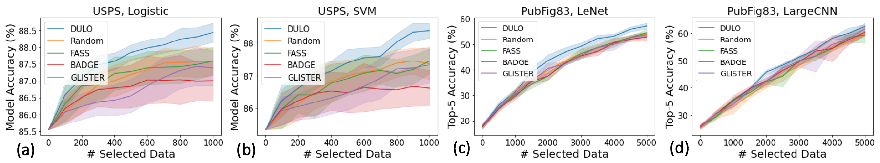
Figure 5: One-round AL on Real-life Datasets.

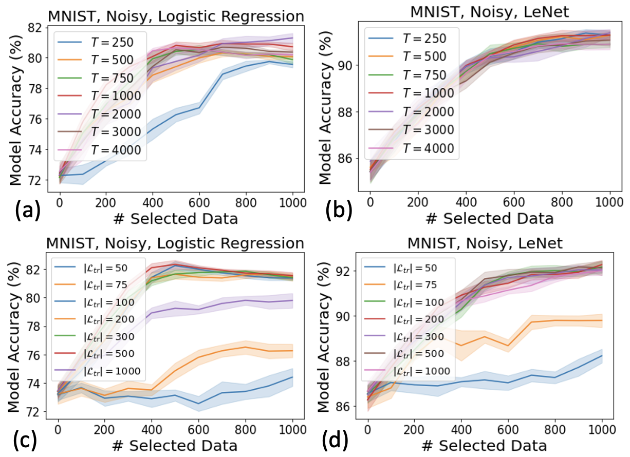
Figure 6: (a) and (b) studies the subset complexity for utility learning. (c) and (d) studies data complexity for utility learning.

Real-life Datasets.

We study the effectiveness of different strategies on real-life datasets, including USPS and PubFig83 datasets, which contain some natural variations in image quality. Figure 5 (a) and (b) show the AL performance on USPS dataset with logistic regression (proxy model) and support vector machine. For both cases, we can see that DULO consistently outperforms all other baselines. Figure 4 (b) illustrates the images selected in different ranks by DULO. We can see that the points selected earlier have higher image quality; especially, the last five selected ‘6’ digit images tend to be blurry and some could easily be confused with other digits. The last ten selected images contain four ‘1’s, which is because USPS is a class-imbalanced dataset, and there are more ‘1’s than other classes. Figure 5 (c) and (d) show the performance on PubFig83 dataset with LeNet (proxy model) and a CNN model. Again, for both cases, we can see that DULO consistently outperforms all other baselines. Figure 4 (c) shows the rankings of 3 images within an optimization block. Interestingly, the early face images selected by DULO contain complete face features, while the later ones either contain more irrelevant features or are corrupted.

Sample Complexity of Data Utility Learning.

There are two kinds of sample complexity involved in the DeepSets-based utility model learning: (1) data complexity which is the size of labeled training dataset $|\mathcal{L}_{tr}|$, and (2) subset complexity which is the number of subsets $T$ for the initially labeled dataset we sample to train proxy models. Both quantities need to be appropriately large to train a utility model that can generalize well to unseen subset and capture the interactions between different data points. Figure 6 (a) and (b) show the one-round AL performance for DeepSets utility models trained with different amount of subset samples. We find that the performance is nearly optimal as long as the number of subset samples is above 500. This is not a large number: training 1000 logistic regression models on MNIST on 300 data points in PyTorch only requires around 30 minutes with NVIDIA Tesla K80 GPU. Since CNN models are more effective on MNIST, even the data utility model trained with only 250 samples is able to achieve comparable performance to the optimal accuracy for learning LeNet.

Figure 6 (c) and (d) show the one-round AL performance for DeepSets utility models trained with different amount of labeled training samples $|\mathcal{L}_{tr}|$. Note that here the largest possible training samples for the proxy model varies, but we still train the classifiers with 300 labeled training samples together with selected data points. We fix the block size and number of subsets sampled for DeepSets training in the experiments. As we can see, near-optimal performance could be achieved even when there are only 100 labeled training data points. When $|\mathcal{L}_{tr}|$ is too large, the trained DeepSets model’s performance might degrade due to insufficient training samples compared with input dimensions. When $|\mathcal{L}_{tr}|$ is too small, the generalizability of DeepSets utility model to large sets would be worse and at the same time, the block size has a small upper limit, which can capture less data interaction. A practical guideline for setting the size of initial labeled dataset is in the level of hundreds.

Conclusion and Limitations

In this paper, we identify an important AL setting where only one round of label query is allowed. The simple extension of existing multi-round batch AL algorithms to one-round cannot maintain descent performance. This work proposes a general framework for one-round AL via data utility function learning and optimization. Our evaluation shows that it outperforms existing baselines across various datasets and models.

There are two assumptions underlying our approach: the labels of the initial labeled dataset is correct and the labeled and unlabeled datasets should share the same set of labels. Extending DULO to noisy initial labeled data and varied label settings would be interesting future directions. Moreover, we would like to complement our currently empirical-only results of approximately submodular data utility and correlated data utility with rigorous analysis, which could provide more guidance on utility model training and proxy model section strategy. Scalability is another limitation of our framework. While the evaluation section shows that both the sample and data complexity for utility learning is acceptable, DULO could still be ineffective for data of very high dimensions because limited initial labeled set does not allow training data utility models with reasonable performance based on proxy models. Further improving the scalability of DULO through some efficient approximation heuristics of data utility functions would be interesting future works.

Appendix A Additional Experiment Settings

Figure 1 in the Main Text

In Figure 1 of the maintext, we use USPS dataset. The MLP we use has 1 hidden layer with 128 neurons, trained with learning rate $10^{-3}$ and batch size 32.

Details of Datasets Used in Section 5

MNIST.

MNIST consists of 70,000 handwritten digits. The images are $28\times 28$ grayscale pixels.

CIFAR-10.

CIFAR-10 consists of 60,000 3-channel images in 10 classes (airplane, automobile, bird, cat, deer, dog, frog, horse, ship and truck). Each image is of size $32\times 32$.

USPS.

USPS is a real-life dataset of 9,298 handwritten digits. The images are $16\times 16$ grayscale pixels. The dataset is class-imbalanced with more $0$ and $1$ than the other digits.

PubFig83.

PubFig83 is a real-life dataset of 13,837 facial images for 83 individuals. Each image is resized to $32\times 32$.

Implementation Details

A small CNN model is used as the proxy model for CIFAR-10 dataset, which has two convolutional layers, each is followed by a max pooling layer and a ReLU activation function. LeNet model is the proxy model for PubFig83 dataset, and we also used it to test the AL performance for MNIST in the experiment. LeNet is adapted from (LeCun et al. 1998), which has two convolutional layers, two max pooling layers and one fully-connected layer. A CNN model is used to evaluate AL performance on CIFAR-10 and PubFig83, which has six convolutional layers, and each of them is followed by a batch normalization layer and a ReLU layer. We use Adam optimizer with learning rate $10^{-3}$, mini-batch size 32 to train all of the aforementioned models for 30 epochs, except that we train LeNet for 5 epochs when using it for testing AL performance on MNIST. We also use the support vector machine (SVM) to evaluate AL performance on the USPS dataset. We implement SVM with scikit-learn (Pedregosa et al. 2011) and set the L2 regularization parameter to be $0.1$.

A DeepSets model is a function $f_{DS}(S)=\rho(\sum_{x\in S}\phi(x))$ where both $\rho$ and $\phi$ are neural networks. In our experiment, both $\phi$ and $\rho$ networks have 3 fully-connected layers. For MNIST and USPS, we set the number of neurons to be 128 in each hidden layer. For CIFAR-10 and PubFig83, we set the number of neurons in every hidden layer to be 512. We set the dimension of set features (i.e., the output of $\phi$ network) for DeepSets models to be 128 in all experiments, except for USPS dataset the set feature number is 64. We use the Adam optimizer with learning rate $10^{-5}$, mini-batch size of 32, $\beta_{1}=0.9$, and $\beta_{2}=0.999$ to train all of the DeepSets utility models.

In terms of the baseline batch AL approaches, we set $\beta$ in FASS to be the size of unlabeled dataset after parameter tuning. We set the learning rate in GLISTER to be 0.05, following the original paper.

Appendix B Additional Experiment Results

Diminishing Return

Figure 7 shows more examples of the “diminishing return” property of data utility functions for commonly used models and datasets. These figures are produced by computing the average marginal contribution of a fixed data point to different base sample sets. As we can see, for all cases we consider, the marginal contribution decreases as the size of the base sample sets increase, which matches the definition of submodularity.

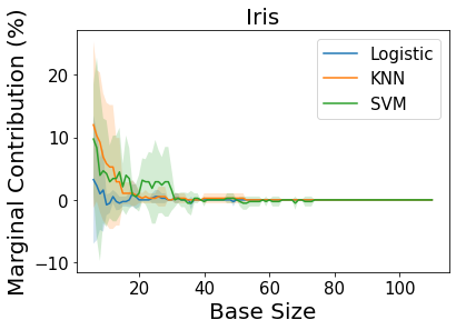
(a)

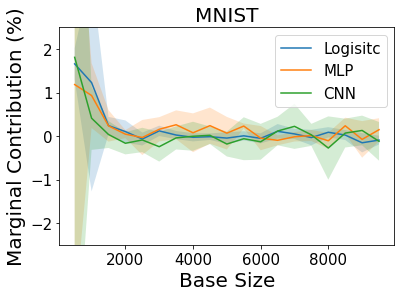
(b)

Figure 7: More examples of the “diminishing return” property of data utility functions for widely used learning algorithms: (a) is trained on Iris dataset, and (b) is trained on MNIST dataset. The marginal contribution is computed in terms of test accuracy. The sampling procedure is the same as what is described in the Caption of Figure 1, except for MNIST dataset (Figure (b)), since the size of the training set $D$ is large, at each iteration we randomly sample 500 data points $K\in D/(S\cup\{j\})$ each time and construct $S_{i}=S_{i-1}\cup\{K\}$. The MLP we use has 1 hidden layer with 128 neurons. The CNN model has two convolutional layers, each is followed by a max pooling layer and a ReLU activation function. Both models are trained with learning rate $10^{-3}$ and batch size 32.

Utility Transferrability

Figure 8 shows more examples of the transferrability of data utilities between different learning algorithms. The dataset here we use is CIFAR-10. For each point in the figures, we randomly sample 5000 CIFAR-10 images and add Gaussian noise to a random portion of the images. We then record the test accuracies of different model architectures trained on the dataset. As we can see, for all cases we tested, the Spearman’s rank correlation coefficients are high in general, which means that the data utilities are strongly positively correlated. This further illustrates the validity of proxy model approach. However, while the transferrability of data utility across different learning algorithms has important applications, its theoretical analysis seem to be a difficult problem as discussed in Wu and Zhang (2021) and it’s certainly an important future research direction.

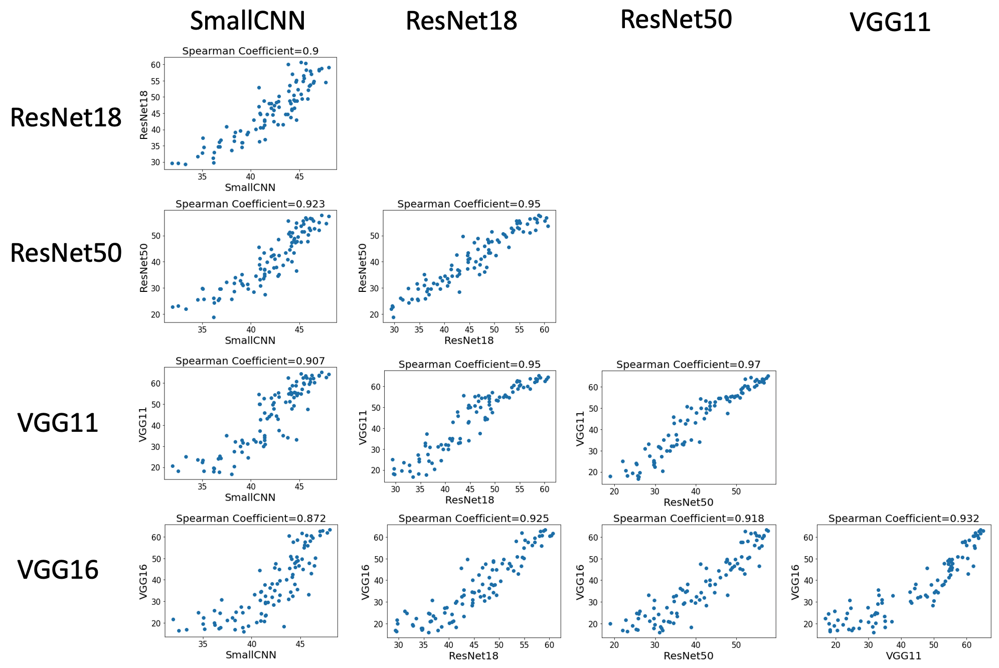
Figure 8: Model Utility Transferrability

Optimization Block Size

Figure 9 (a) shows the one-round AL performance with different optimization block sizes $B$. As we can see, both too small and too large block size can degrade the selected data’s utility. When $B$ is too small, DeepSets fails to capture interactions between data points selected from different blocks. When $B$ is too large, DeepSets has large generalization error.

Although the stochastic optimization algorithm runs in $O(|\mathcal{U}|)$ regardless of the block size (without parallelization), individual DeepSets evaluation time increases significantly with a larger input set. Figure 9 (b) shows the runtime vs accuracy plot with different block sizes. We can see that when $B$ is too large, it suffers from both poor utility and inefficiency. However, we find a wide range of $B$ that achieves both good efficiency and high data utility (the points located on the right of the figure), which is around $|\mathcal{L}_{tr}|$ ($|\mathcal{L}_{tr}|=500$ for CIFAR-10 in our setting). This servers as a heuristic choice of $B$. In this range, the block size is small enough so that DeepSets models generalize well on input sets of block sizes, while also being large enough so that the utility model could capture most of the data interactions.

Figure 9: Ablation Study: (a) compares DULO’s performance with different optimization block sizes, and (b) studies the relationship between efficiency and AL performance for different block sizes when the number of selected data is 6000.

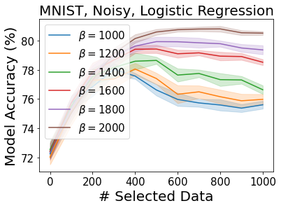
(a)

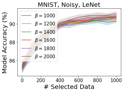
(b)

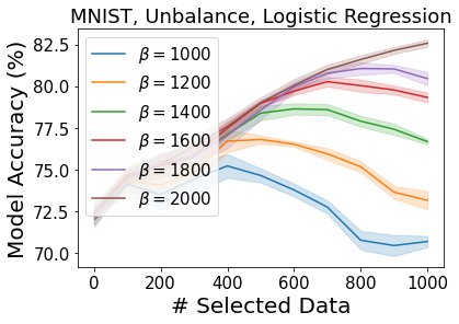
(c)

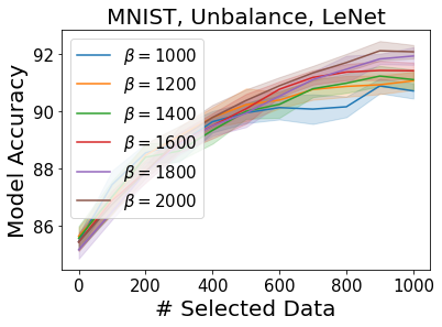
(d)

Figure 10: Ablation Study: the performance of DULO when we run greedy optimization on the $\beta$ most uncertain samples of the current classifiers.

Combining with Uncertainty Sampling

Traditionally, AL techniques like uncertainty sampling (US) and query by committee (QBC) have shown great promise in several domains of machine learning (Settles 2009). However, in the task of multi-round batch AL, naive uncertainty sampling fails to capture the interactions between selected samples. Simply choosing the most uncertain samples may lead to a selected set with very low diversity. Filtered Active Submodular Selection (FASS) (Wei, Iyer, and Bilmes 2015) combines the uncertainty sampling method with a submodular data subset selection framework. Specifically, at every round $t$, FASS first selects a candidate set of $\beta_{t}$ most uncertain samples among unlabeled data, and then runs greedy optimization on an appropriate submodular objective (with the hypothesized labels assigned by the current model). It is natural to ask whether we should also combine DULO with uncertainty sampling by only performing greedy optimization on the most uncertain samples. We evaluate the performance of DULO when we first filter out data points that the current classifier has high confidence about, and preserve a candidate set of $\beta$ most uncertain samples on which we run stochastic greedy optimization. We show the performance of different values of $\beta$ on class-imbalanced and noisy MNIST dataset in Figure 10, where $\beta=|\mathcal{U}|=2000$ coincides with the setting of the original DULO algorithm. As we can see, for all settings studied in our experiments, $\beta=2000$ consistently outperforms other smaller values of $\beta$. Hence, using uncertainty sampling to pre-process unlabeled samples does not seem to lead to better performance in our one-round AL framework. We conjecture that this is because we only have very few labeled samples at the beginning. In that case, the performance of the initial classifiers is pretty poor and their uncertainty outputs are not informative.

References

- Alpaydin and Kaynak (1998) Alpaydin, E.; and Kaynak, C. 1998. Optical recognition of handwritten digits data set. UCI Machine Learning Repository.
- Ash et al. (2019a) Ash, J. T.; Zhang, C.; Krishnamurthy, A.; Langford, J.; and Agarwal, A. 2019a. Deep batch active learning by diverse, uncertain gradient lower bounds. arXiv preprint arXiv:1906.03671.
- Ash et al. (2019b) Ash, J. T.; Zhang, C.; Krishnamurthy, A.; Langford, J.; and Agarwal, A. 2019b. Deep batch active learning by diverse, uncertain gradient lower bounds. arXiv preprint arXiv:1906.03671.
- Bairi et al. (2015) Bairi, R.; Iyer, R.; Ramakrishnan, G.; and Bilmes, J. 2015. Summarization of multi-document topic hierarchies using submodular mixtures. In Proceedings of the 53rd Annual Meeting of the Association for Computational Linguistics and the 7th International Joint Conference on Natural Language Processing (Volume 1: Long Papers), 553–563.
- Balcan and Harvey (2011) Balcan, M.-F.; and Harvey, N. J. 2011. Learning submodular functions. In Proceedings of the forty-third annual ACM symposium on Theory of computing, 793–802.
- Brown et al. (2020) Brown, T. B.; Mann, B.; Ryder, N.; Subbiah, M.; Kaplan, J.; Dhariwal, P.; Neelakantan, A.; Shyam, P.; Sastry, G.; Askell, A.; et al. 2020. Language models are few-shot learners. arXiv preprint arXiv:2005.14165.
- Buchbinder et al. (2014) Buchbinder, N.; Feldman, M.; Naor, J.; and Schwartz, R. 2014. Submodular maximization with cardinality constraints. In Proceedings of the twenty-fifth annual ACM-SIAM symposium on Discrete algorithms, 1433–1452. SIAM.
- Campbell et al. (2000) Campbell, C.; Cristianini, N.; Smola, A.; et al. 2000. Query learning with large margin classifiers. In ICML, volume 20, 0.
- Feige (1998) Feige, U. 1998. A threshold of ln n for approximating set cover. Journal of the ACM (JACM), 45(4): 634–652.
- Feldman, Kothari, and Vondrák (2020) Feldman, V.; Kothari, P.; and Vondrák, J. 2020. Tight bounds on l1 approximation and learning of self-bounding functions. Theoretical Computer Science, 808: 86–98.
- Feldman and Vondrák (2016) Feldman, V.; and Vondrák, J. 2016. Optimal bounds on approximation of submodular and XOS functions by juntas. SIAM Journal on Computing, 45(3): 1129–1170.
- Fine, Gilad-Bachrach, and Shamir (2002) Fine, S.; Gilad-Bachrach, R.; and Shamir, E. 2002. Query by committee, linear separation and random walks. Theoretical Computer Science, 284(1): 25–51.
- Freund et al. (1997) Freund, Y.; Seung, H. S.; Shamir, E.; and Tishby, N. 1997. Selective sampling using the query by committee algorithm. Machine learning, 28(2): 133–168.
- Graepel and Herbrich (2000) Graepel, T.; and Herbrich, R. 2000. The kernel gibbs sampler. In NIPS, 514–520. Citeseer.
- Hassidim and Singer (2018) Hassidim, A.; and Singer, Y. 2018. Optimization for approximate submodularity. In Proceedings of the 32nd International Conference on Neural Information Processing Systems, 394–405.
- Hoi et al. (2006) Hoi, S. C.; Jin, R.; Zhu, J.; and Lyu, M. R. 2006. Batch mode active learning and its application to medical image classification. In Proceedings of the 23rd international conference on Machine learning, 417–424.
- Horel and Singer (2016) Horel, T.; and Singer, Y. 2016. Maximization of approximately submodular functions. Advances in Neural Information Processing Systems, 29: 3045–3053.
- Jia et al. (2019) Jia, R.; Dao, D.; Wang, B.; Hubis, F. A.; Gurel, N. M.; Li, B.; Zhang, C.; Spanos, C. J.; and Song, D. 2019. Efficient task-specific data valuation for nearest neighbor algorithms. arXiv preprint arXiv:1908.08619.
- Killamsetty et al. (2020) Killamsetty, K.; Sivasubramanian, D.; Ramakrishnan, G.; and Iyer, R. 2020. GLISTER: Generalization based Data Subset Selection for Efficient and Robust Learning. arXiv preprint arXiv:2012.10630.
- Kirsch, Van Amersfoort, and Gal (2019) Kirsch, A.; Van Amersfoort, J.; and Gal, Y. 2019. Batchbald: Efficient and diverse batch acquisition for deep bayesian active learning. arXiv preprint arXiv:1906.08158.
- Krizhevsky, Hinton et al. (2009) Krizhevsky, A.; Hinton, G.; et al. 2009. Learning multiple layers of features from tiny images.
- LeCun (1998) LeCun, Y. 1998. The MNIST database of handwritten digits. http://yann. lecun. com/exdb/mnist/.
- LeCun et al. (1998) LeCun, Y.; Bottou, L.; Bengio, Y.; and Haffner, P. 1998. Gradient-based learning applied to document recognition. Proceedings of the IEEE, 86(11): 2278–2324.
- Lewis and Gale (1994) Lewis, D. D.; and Gale, W. A. 1994. A sequential algorithm for training text classifiers. In SIGIR’94, 3–12. Springer.
- Minoux (1978) Minoux, M. 1978. Accelerated greedy algorithms for maximizing submodular set functions. In Optimization techniques, 234–243. Springer.
- Mirzasoleiman et al. (2015) Mirzasoleiman, B.; Badanidiyuru, A.; Karbasi, A.; Vondrák, J.; and Krause, A. 2015. Lazier than lazy greedy. In Proceedings of the AAAI Conference on Artificial Intelligence, volume 29.
- Paszke et al. (2019) Paszke, A.; Gross, S.; Massa, F.; Lerer, A.; Bradbury, J.; Chanan, G.; Killeen, T.; Lin, Z.; Gimelshein, N.; Antiga, L.; et al. 2019. Pytorch: An imperative style, high-performance deep learning library. arXiv preprint arXiv:1912.01703.
- Pedregosa et al. (2011) Pedregosa, F.; Varoquaux, G.; Gramfort, A.; Michel, V.; Thirion, B.; Grisel, O.; Blondel, M.; Prettenhofer, P.; Weiss, R.; Dubourg, V.; et al. 2011. Scikit-learn: Machine learning in Python. the Journal of machine Learning research, 12: 2825–2830.
- Pinto et al. (2011) Pinto, N.; Stone, Z.; Zickler, T.; and Cox, D. 2011. Scaling up biologically-inspired computer vision: A case study in unconstrained face recognition on facebook. In CVPR 2011 WORKSHOPS, 35–42. IEEE.
- Schohn and Cohn (2000) Schohn, G.; and Cohn, D. 2000. Less is more: Active learning with support vector machines. In ICML, volume 2, 6. Citeseer.
- Sener and Savarese (2017) Sener, O.; and Savarese, S. 2017. Active learning for convolutional neural networks: A core-set approach. arXiv preprint arXiv:1708.00489.
- Settles (2009) Settles, B. 2009. Active learning literature survey.
- Seung, Opper, and Sompolinsky (1992) Seung, H. S.; Opper, M.; and Sompolinsky, H. 1992. Query by committee. In Proceedings of the fifth annual workshop on Computational learning theory, 287–294.
- Tong and Koller (2001) Tong, S.; and Koller, D. 2001. Support vector machine active learning with applications to text classification. Journal of machine learning research, 2(Nov): 45–66.
- Wang, Yang, and Jia (2021) Wang, T.; Yang, Y.; and Jia, R. 2021. Learnability of Learning Performance and Its Application to Data Valuation. arXiv preprint arXiv:2107.06336.
- Wei, Iyer, and Bilmes (2014) Wei, K.; Iyer, R.; and Bilmes, J. 2014. Fast multi-stage submodular maximization. In International conference on machine learning, 1494–1502. PMLR.
- Wei, Iyer, and Bilmes (2015) Wei, K.; Iyer, R.; and Bilmes, J. 2015. Submodularity in data subset selection and active learning. In International Conference on Machine Learning, 1954–1963. PMLR.
- Wei et al. (2014) Wei, K.; Liu, Y.; Kirchhoff, K.; and Bilmes, J. 2014. Unsupervised submodular subset selection for speech data. In 2014 IEEE International Conference on Acoustics, Speech and Signal Processing (ICASSP), 4107–4111. IEEE.
- Wu and Zhang (2021) Wu, W.; and Zhang, C. 2021. Towards understanding end-to-end learning in the context of data: machine learning dancing over semirings & Codd’s table. In Proceedings of the Fifth Workshop on Data Management for End-To-End Machine Learning, 1–4.
- Zaheer et al. (2017) Zaheer, M.; Kottur, S.; Ravanbakhsh, S.; Poczos, B.; Salakhutdinov, R.; and Smola, A. 2017. Deep sets. arXiv preprint arXiv:1703.06114.