Unconventional low temperature features in the one-dimensional frustrated $q$-state Potts model

Abstract

Here we consider a one-dimensional $q$-state Potts model with an external magnetic field and an anisotropic interaction that selects neighboring sites that are in the spin state 1. The present model exhibits an unusual behavior in the low-temperature region, where we observe an anomalous vigorous change in the entropy for a given temperature. There is a steep behavior at a given temperature in entropy as a function of temperature, quite similar to first-order discontinuity, but there is no jump in the entropy. Similarly, second derivative quantities like specific heat and magnetic susceptibility also exhibit a strong acute peak rather similar to second-order phase transition divergence, but once again there is no singularity at this point. Correlation length also confirms this anomalous behavior at the same given temperature, showing a strong and sharp peak which easily one may confuse with a divergence. The temperature where occurs this anomalous feature we call pseudo-critical temperature. We have analyzed physical quantities, like correlation length, entropy, magnetization, specific heat, magnetic susceptibility, and distant pair correlation functions. Furthermore, we analyze the pseudo-critical exponent that satisfy a class of universality previously identified in the literature for other one-dimensional models, these pseudo-critical exponents are: for correlation length $\nu=1$, specific heat $\alpha=3$ and magnetic susceptibility $\mu=3$.

I Introduction

The advantage of exactly solvable models is its easy handling to analyze several properties, which can show interesting features despite it is simplicity. In contrast, more detailed models are rarely exactly solvable, and it would restrict us to performing only through numerical computations, which prevents further analysis of these types of models. Some one-dimensional models[1] can help us understand and predict leading behavior in more complex models. From the experimental side, one-dimensional models accurately describe several chemical compounds[2, 3]. That is why the one-dimensional models are quite important to investigate, both from theoretical and experimental points of view.

Earlier in the fifties, van Hove[4] proposed a theorem to verify the absence of phase transition in uniform one-dimensional models with short-range interaction. The validity of the proposed theorem follows the conditions: (i) homogeneity, (ii) the Hamiltonian should not include particles positions terms (like external fields). (iii) hard-core particles. Based on the Perron-Frobenius theorem [5], condition, the van Hove theorem[4] is restricted to limited one-dimensional systems. Later, Cuesta and Sanchez[6] tried to extend the theorem of non-existence phase transition for a more general one-dimensional system. Mainly, they included an external field and considered point-like particles, which extends the theorem. Even with this extension, it is still far from being a fully general theorem of non-existence phase transition.

There are unusual one-dimensional models with a short-range coupling that exhibit a phase transition at finite temperature. The zipper or Kittel model [7], which is one of the simplest models with a finite size transfer matrix that exhibits a first-order phase transition. Another model, considered by Chui-Wicks[8], is typical of models called solid-on-solid for surface growth. It has the infinite dimension transfer-matrix and is exactly solvable. Because of the impenetrable condition of the subtract, the model shows the existence of a finite temperature phase transition. One more model is that considered by Dauxois-Peyrard[9], with an infinite dimension transfer matrix, which can be explored numerically. Lately, Sarkanych et al.[10] proposed a one-dimensional Potts model with invisible states and short-range coupling. The term invisible means an additional energy degeneracy, which only contributes to the entropy, but not the interaction energy. They named these states the invisible states, which generate the first-order phase transition.

Motivated by low-dimensional systems, such as the simple zipper model[7] that describes the long-chain nucleotides of deoxyribonucleic acid (DNA), Zimm and Bragg[11] introduced an essentially phenomenological cooperative parameter, which provides narrow helix-coil transitions. Since that several investigations were driven in the literature[12, 13, 14, 15]. Cooperative systems in one-dimension can be well represented by Potts-like models[12, 14], where the helix-coil transition in polypeptides[13] can be studied, which is a typical application of theoretical physics to macromolecular systems, the results of which are quite appropriate to understand the physical properties of the helix-coil transition. The polycyclic aromatic surface elements of the carbon nanotube (CNT) and the aromatic DNA provide reversible adsorption. Tonoyan et al.[15] adapted the Hamiltonian of the zipper model in order to take into account the DNA-CNT interactions.

Potts model is a generalization of the Ising model to more than two components, such as interacting spins in a crystalline lattice. Standard $q$-state Potts model [16], with $q\geqslant 2$ has been assumed as an integer denoting the number of states of each site. Potts model is quite relevant in statistical physics. In some crystal-lattices would occur vacancies, which leads to a site diluted Potts model. The site dilute $q$-state Potts model[17, 18] is equivalent to $q+1$-state standard Potts model[16]. Chaves and Riera[19] investigated a particular case of dilute Potts chain. Recently, a different dilute Ising spin-1 chain[20] was also studied in the framework of the projection operator.

An unusual property called pseudo-transition was observed in some recent works: Like in a double-tetrahedral chain of localized Ising spins with mobile electrons showing a strong thermal excitation that easily suggests the existence of a first-order phase transition[21, 22, *galisova20]. Similarly, the frustrated spin-1/2, Ising-Heisenberg’s three-leg tube exhibited a pseudo-transition[24]. In reference [25], this property was also observed when studying the specific heat, where reported a sharp peak on the spin-1/2 Ising-Heisenberg ladder with alternating Ising and Heisenberg inter-leg couplings. This weird property was even observed in the spin-1/2 Ising diamond chain in the neighboring of the pseudo-transition[26]. Besides, deeper investigations were performed on this peculiar property in [27]. Additionally, the distant correlation functions have been studied around pseudo-transition for a spin-1/2 Ising-XYZ diamond chain[28]. A bit different proposal to identify the pseudo-transition in one-dimensional models[29, *Rojas2020] was explored in the framework of the phase boundary residual entropy relationship with the finite temperature pseudo-transition. Further investigation around the pseudo-transition was also focused on the universality and pseudo-critical exponents of one-dimensional models[31].

We organize the article as follows. In Section II we present the model and analyze the zero-temperature phase diagrams. In Section III, we study the thermodynamics of the model and explore an anomalous phenomenon called pseudo-transition for several physical quantities. In Section IV, we investigate the manifest of the pseudo-transition in terms of the distant pair correlation functions and correlation length. The pseudo critical exponents for the correlation length, specific heat, and susceptibility we discuss in Section V. Finally, in Section VI, we present our conclusions.

II The frustrated Potts chain

Let us consider a Potts model[16], here we assume the one-dimensional case, whose Hamiltonian becomes

$$H=-\sum_{i=1}^{N}\left\{J\delta_{\sigma_{i},\sigma_{i+1}}+K\delta_{\sigma_{i},1}\delta_{1,\sigma_{i+1}}+h\delta_{\sigma_{i},1}\right\},$$ (1)

with $\sigma=\left\{1,\ldots q\right\}$. Whereas $J$ is bound coupling parameter, $h$ denotes the external field aligned to state 1, and $K$ denotes the parameter of an anisotropic interaction that selects neighboring sites that are in the spin state 1.

The Hamiltonian (1) for the case $q=2$, like standard Potts model drops into spin-1/2 Ising chain model. For the case of $q\geqslant 3$, the model becomes a frustrated system for certain choices of parameters, as shown below.

It is worth notice that the Hamiltonian (1) can also be equivalent to a diluted Potts model with $q-1$ states, as demonstrated by Wu [16]. The features of the critical properties of the two-dimensional diluted Potts model were studied earlier using Fortuin-Kasteleyn clusters [32] and the transfer matrix method [33].

II.1 Zero temperature phase diagram

In order to analyze the phase diagram of $q$-state Potts model at zero temperature, we identify four ground states assuming $q\geqslant 3$ for the model (1), which read below

$$|FM_{1}\rangle= \prod_{i=1}^{N}\bigl{(}|1\rangle_{i}\bigr{)},$$ (2)

$$|FM_{2}\rangle= \prod_{i=1}^{N}\bigl{(}|j\rangle_{i}\bigr{)},\quad j=\{2,\dots,q\},$$ (3)

$$|FR_{1}\rangle= \prod_{i=1}^{N/2}\left(|1\rangle_{2i-1}|\sigma_{i}\rangle_{2i}\right),$$ (4)

$$|FR_{2}\rangle= \prod_{i=1}^{N}\left(|\sigma_{i}\rangle\right),\quad\sigma_{i}\neq\sigma_{i\pm 1},$$ (5)

where $\sigma_{i}=\{2,\dots,q\}$. Additional information, concerning phases and phase-boundaries, are listed in Table 1 for different physical quantities at zero temperature, like magnetization, entropy, and pair distribution functions (PDF), which can be obtained by taking the limit of $T\rightarrow 0$ of the quantities (23), (55) and (67).

In Fig. 1a is illustrated schematically the ground state phase diagram in the plane $J-h$, for the Hamiltonian (1) assuming $K<0$. Here we observe four phases illustrated above. Similarly, in panel (b) and (c) are illustrated alternative phase diagrams for $K=0$ and $K>0$, respectively.

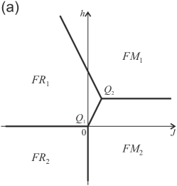
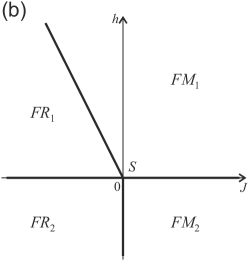
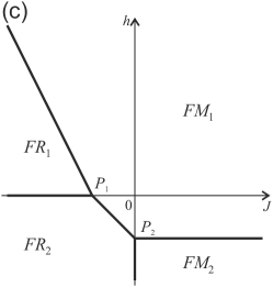
Figure 1: The ground state phase diagrams of the $q$-state Potts chain with Hamiltonian (1) for $q\geqslant 3$. (a) $K<0$, (b) $K=0$, and (c) $K>0$. Here the points are: $Q_{1}(0,0)$, $Q_{2}(-K/2,-K)$, $S(0,0)$, $P_{1}(-K,0)$, $P_{2}(0,-K)$.

The first state is a type of ferromagnetic ($FM_{1}$) phase where all sites are in state $\sigma_{i}=1$, with energy per spin $E_{FM_{1}}=-(J+K+h)$. The second state is another type of "ferromagnetic" ($FM_{2})$ phase with energy $E_{FM_{2}}=-J$. The average fraction of pairs of adjacent spins in the same state $\mu$, where $\mu=2,\ldots q$, is PDF $g_{\mu,\mu}^{(1)}=1/(q-1)$ (see Table 1). At the same time, $g_{\mu,\mu^{\prime}}^{(1)}=0$, where $\mu\neq\mu^{\prime}$, which means that in the thermodynamic limit, the fraction of pairs with different spin states and their contribution to the energy of the system are equal to zero. This implies that, in the general case, the $FM_{2}$ phase consists of $q-1$ sorts of equivalent macroscopic ferromagnetic domains with spins in the $\mu$ state. Equation (3) corresponds to the single-domain case. The entropy of both $FM_{1}$ and $FM_{2}$ phases is zero. The third is a type frustrated ($FR_{1}$) phase, with alternating sites are in states $\sigma_{2i-1}=1$, while the other sites $\sigma_{2i}$ can take $\sigma_{2i}=2,\ldots q$, and the corresponding energy is $E_{FR_{1}}=-h/2$. This phase state is frustrated at $q>2$. Due to every second site can be in any of the $q-1$ states, the entropy per spin is equal to $\mathcal{S}=\frac{1}{2}\ln(q-1)$. The fourth state is another type of frustrated ($FR_{2}$) phase, in each site $\sigma_{i}$ can take independently $\sigma_{i}=\{2,\dots,q\}$ but $\sigma_{i}\neq\sigma_{i\pm 1}$, whose corresponding energy is $E_{FR_{2}}=0$. In this case, each subsequent site of the chain can be in one of $q-2$ states, and the entropy is equal to $\mathcal{S}=\ln(q-2)$. If $q>3$, the $FR_{2}$ phase is evidently frustrated state. Although, for $q=3$, there is an alternation of sites in states $\sigma_{i}=2$ and $\sigma_{i}=3$, and the entropy of the $FR_{2}$ phase is zero.

It is important to note that two different situations can occur at phase boundaries. The first case is when the states of two adjacent phases are mixed at the microscopic level. For example, for the $FR_{1}$-$FM_{1}$ boundary, the $FR_{1}$ state of any pair of sites can be changed to the $FM_{1}$ state, and vice versa. Such a replacement does not lead to the appearance of microscopic states from other phases, and the energy of the system does not change. As a result, the entropy of such a mixed state at the phase boundary is greater than the entropy of the adjacent phases. A similar situation is observed for the boundaries $FR_{1}$-$FR_{2}$, $FR_{2}$-$FM_{2}$, and $FR_{1}$-$FM_{2}$ at $K<0$. In the second case, it can be a pure state of one of the adjacent phases, or the phase separation, when each phase is represented by the macroscopic domains. So, on the $FR_{2}$-$FM_{1}$ boundary for $K>0$, the replacement for a pair of neighboring nodes in state $FR_{2}$ by state $FM_{1}$ leads to the appearance of $FR_{1}$ states, which are energetically unfavorable. A similar situation occurs at the $FM_{1}$-$FM_{2}$ boundary. Note that in the $FM_{1}$-$FM_{2}$ interface curve the residual entropy is zero.

III Thermodynamics

The frustrated $q$-state Potts model Hamiltonian (1) can be solved through transfer matrix technique, which results in a $q$-dimensional matrix, given by

$$\mathbf{V}=\begin{pmatrix}d_{1}&t_{1}&t_{1}&\cdots&t_{1}&t_{1}\\ t_{1}&d_{2}&t_{2}&\cdots&t_{2}&t_{2}\\ t_{1}&t_{2}&d_{2}&\cdots&t_{2}&t_{2}\\ \vdots&\vdots&\vdots&\ddots&\vdots&\vdots\\ t_{1}&t_{2}&t_{2}&\cdots&d_{2}&t_{2}\\ t_{1}&t_{2}&t_{2}&\cdots&t_{2}&d_{2}\end{pmatrix},$$ (6)

where $d_{1}=xkz$, $d_{2}=x$, $t_{1}=\sqrt{z}$, $t_{2}=1$, and $x=\mathrm{e}^{\beta J}$, $k=\mathrm{e}^{\beta K}$, $z=\mathrm{e}^{\beta h}$.

Let us write the transfer matrix eigenvalues similarly to that defined in reference [27], that being so, we have

$$\lambda_{1}= \,\frac{1}{2}\left(w_{1}+w_{-1}+\sqrt{(w_{1}-w_{-1})^{2}+4w_{0}^{2}}\right),$$ (7)

$$\lambda_{2}= \,\frac{1}{2}\left(w_{1}+w_{-1}-\sqrt{(w_{1}-w_{-1})^{2}+4w_{0}^{2}}\right),$$ (8)

$$\lambda_{j}= \,d_{2}-t_{2},\quad j=\{3,4,\dots,q\},$$ (9)

where

$$w_{1} = d_{1},$$ (10)

$$w_{-1} = d_{2}+\left(q-2\right)t_{2},$$ (11)

$$w_{0} = \sqrt{q-1}\,t_{1}.$$ (12)

The corresponding transfer matrix eigenvectors are

$$|u_{1}\rangle= \cos(\phi)|1\rangle+\tfrac{\sin(\phi)}{\sqrt{q-1}}\sum_{\mu=2}^{q}|\mu\rangle,$$ (13)

$$|u_{2}\rangle= -\sin(\phi)|1\rangle+\tfrac{\cos(\phi)}{\sqrt{q-1}}\sum_{\mu=2}^{q}|\mu\rangle,$$ (14)

$$|u_{j}\rangle= \sqrt{\tfrac{j-2}{j-1}}\Bigl{(}\tfrac{1}{j-2}\sum_{\mu=2}^{j-1}|\mu\rangle-|j\rangle\Bigr{)},\quad j=\{3,\cdots,q\},$$ (15)

where $\phi=\frac{1}{2}\cot^{-1}\left(\frac{w_{1}-w_{-1}}{2w_{0}}\right)$, with $-\frac{\pi}{4}\leqslant\phi\leqslant\frac{\pi}{4}$.

By using the transfer matrix eigenvalues, we express the partition function as follows

$$Z_{N}= \,\lambda_{1}^{N}+\lambda_{2}^{N}+(q-2)\lambda_{3}^{N}$$

$$= \,\lambda_{1}^{N}\left\{1+\Bigl{(}\tfrac{\lambda_{2}}{\lambda_{1}}\Bigr{)}^{N}+(q-2)\Bigl{(}\tfrac{\lambda_{3}}{\lambda_{1}}\Bigr{)}^{N}\right\}.$$ (16)

It is evident that the eigenvalues satisfy the following relation $\lambda_{1}>\lambda_{2}\geqslant\lambda_{3}$. Hence, assuming $q$ finite, the free energy per spin in thermodynamic limit reduces to

$$f=-T\ln\left(\lambda_{1}\right).$$ (17)

Note that the free energy is a continuous function with no singularity or discontinuity, thus we do not expect any real phase transition at finite temperature.

III.1 Pseudo-Critical temperature

Recently pseudo-critical temperature has been discussed in Ising and Ising-Heisenberg spin models[21, 24, 25, 27], in several one-dimensional spin models.

To find pseudo-critical temperature, we follow the same strategy to that used in reference[27]. In our case the largest eigenvalues has the same structure to that found in reference[27], so necessary conditions for a pseudo-transition are met, if $w_{1}\sim w_{-1}\ggg w_{0}$, $|w_{1}-w_{-1}|\gg w_{0}$. The pseudo-transition point can be obtained when the first term inside the square root of $\lambda_{1}$ given by eq.(7) turns to zero, which gives

$$e^{\frac{J+K+h}{T_{p}}}=q-2+e^{\frac{J}{T_{p}}}.$$ (18)

In principle, using the above relation, one can find the critical temperature as a function of some Hamiltonian parameters.

The $q$-state Potts chain does not exhibit a real spontaneous long range order at finite temperature since its one-dimensional character. Therefore we define a term “quasi” to refer low temperature regions mainly dominated by ground state configuration. Hence $FR_{2}$ in low temperature region is called as $qFR_{2}$, and so on. As shown in [29, *Rojas2020], pseudo-transitions occur for states near those phase boundaries whose residual entropy is a continuous function of the model parameters for at least one of the adjacent phases. As discussed earlier, the state of the $FR_{2}-FM_{1}$ boundary coincides with the $FR_{2}$ state, so for the $qFR_{2}-qFM_{1}$ boundary, we get from eq.(18) the following relation

$${\rm e}^{\frac{K+h}{T_{p}}}={\rm e}^{-\frac{J}{T_{p}}}(q-2)+1,$$ (19)

which we can simplify and write approximately in the form

$$T_{p}=\frac{J+K+h}{\ln\left(q-2\right)}.$$ (20)

This is the known expression [21, 24, 27, 29, *Rojas2020] for the pseudo-transition temperature:

$$E_{FM_{1}}-E_{FR_{2}}=T_{p}\left(\mathcal{S}_{FR_{2}}-\mathcal{S}_{FM_{1}}\right),$$ (21)

where the energy and entropy per unit cell are given at zero temperature. Since $E_{FM_{1}}=E_{FR_{2}}$ at the $qFR_{2}$-$qFM_{1}$ boundary, $T_{p}$ tends to zero near to it.

Another phase boundary we focus is $qFM_{2}$-$qFM_{1}$. It is worth to mention that, the entropy of the $FM_{1}$ and $FM_{2}$ phases is zero, so the entropy is a continuous function for both adjacent phases. For the $qFM_{2}$-$qFM_{1}$ boundary the eq.(18) can be approximately written in the following form

$$\frac{1}{T_{p}}\left(K+h\right)e^{J/T_{p}}=q-2.$$ (22)

Figure 2: Density plot: (a) for entropy in the plane $T-h$, for $K=1$ and $J=-0.5$. (b) Magnetization $m_{1}$ for the same set of parameters to the panel (a). In (c) entropy in the plane $T-h$ for fixed $K=1$, $J=0.99$. In (d) magnetization for the same set of parameter to the panel (c).

In Fig. 2a is reported the density plot of entropy in the plane $T-h$, assuming fixed parameters $K=1$, $J=-0.5$. Dashed curve describes the boundary $qFR_{2}$-$qFM_{1}$, which corresponds to the pseudo-critical temperature $T_{p}$ as a function of $h$, according eq.(19). It can be seen that the curve is an almost straight line well represented by (20). We can observe also how the sharp boundary between quasi-phase melts smoothly for higher temperature. Similar density plot is depicted in panel(b) for the magnetization $m_{1}$ in the plane $T-h$ for the same set of parameters in panel (a). Analogously, we analyze the phase boundary between $qFM_{2}-qFM_{1}$ in panel (c), assuming fixed parameters $K=1$, $J=0.99$ and $T=0.01$. The dashed line is given by eq.(19) and nicely approximated by (22), since there is no residual entropy in the boundary the quasi-phase $qFM_{1}$ and $qFM_{2}$ leads to zero when temperature vanishes, by looking entropy we cannot distinguishes the boundary of quasi-phase. However, in panel (d) we illustrate the density plot of magnetization $m_{1}$, for the same set of parameters to the panel (c), and we observe clearly a sharp boundary between $qFM_{1}$ and $qFM_{2}$ regions, and this boundary melts smoothly as soon as temperature increases.

III.2 Entropy and Specific heat

The entropy and the specific heat of the system can be obtained from the free energy (17) by

$$\mathcal{S}=-\frac{\partial f}{\partial T},\qquad C=-T\frac{\partial^{2}f}{\partial T^{2}}.$$ (23)

Of particular interest is the behavior of thermodynamic characteristics near the pseudo-transition point. The general method for considering this issue was developed in Ref. [31]. For the one-dimensional Potts model, it is possible to find an explicit form of approximation of the free energy and other thermodynamic quantities near $T_{p}$. Assuming that $\tau=(T-T_{p})/T_{p}\ll 1$ and taking into account the equation (18), we can write

$$w_{1}= \;e^{\beta(J+K+h)}=\tilde{w}_{1}^{\frac{1}{1+\tau}}\approx\tilde{w}_{1}\left(1-\ln\tilde{w}_{1}\,\tau\right),$$ (24)

$$w_{-1}= \;q-2+e^{\beta J}=q-2+x_{p}^{\frac{1}{1+\tau}}\approx\tilde{w}_{1}-x_{p}\ln x_{p}\,\tau,$$ (25)

where

$$\tilde{w}_{1}=\left.w_{1}\right|_{\tau=0}=q-2+x_{p},$$ (26)

and we define the parameters $x_{p}=e^{J/T_{p}}$ and $k_{p}=e^{K/T_{p}}$. The value of $w_{1}-w_{-1}$ is zero at $\tau=0$ due to equation (18), so we get

$$w_{1}-w_{-1}\approx-\tilde{w}_{1}\,a\,\tau,$$ (27)

where we introduce the parameter $a$ as

$$a=\ln\tilde{w}_{1}-\frac{x_{p}\ln x_{p}}{\tilde{w}_{1}}.$$ (28)

Note that the parameter $a^{-1}$ define the slope of the pseudo-transition curve in the plane $T-h$ (see Fig. 2a,c), $dT_{p}/dh=a^{-1}$.

The condition $|w_{1}-w_{-1}|\gg w_{0}$ which is met in the vicinity of $T_{p}$ causes quasi-singular behaviour of the derivative of square root in equations (7,8) at $\tau=0$. Assuming this is the case, we can write the approximation

$$4w_{0}^{2}=4(q-1)e^{\beta h}\approx 4(q-1)\frac{\tilde{w}_{1}}{x_{p}k_{p}}.$$ (29)

This allows us to write eigenvalues (7,8) near $\tau=0$ as

$$\lambda_{1,2}\approx\tilde{w}_{1}\left[1+\left(\tfrac{1}{2}a\tau-\ln\tilde{w}_{1}\right)\tau\pm\tfrac{1}{2}\sqrt{a^{2}\tau^{2}+b^{2}}\right],$$ (30)

where $b^{2}=4w_{0}^{2}/\tilde{w}_{1}^{2}$, and yields the approximation for the free energy (17) in the vicinity of $T_{p}$:

$$f\approx-T_{p}\left[\ln\tilde{w}_{1}-\tfrac{1}{2}a\tau+\tfrac{1}{2}\sqrt{a^{2}\tau^{2}+b^{2}}\right].$$ (31)

The expressions (30,31) being exact at $\tau=0$ have a small deviation from rigorous expansions of $\lambda_{1,2}$ and $f$ in the tiny vicinity $0<|\tau|<\ln(x_{p}k_{p})\,b^{2}/a^{2}\lll 1$ due to the neglect of linear terms in equation (29), but well approximate the functions $\lambda_{1,2}$ and $f$ at $\ln(x_{p}k_{p})\,b^{2}/a^{2}<|\tau|\ll 1/|\ln x_{p}|$. This implies a simple necessary condition for a pseudo-transition in the form $b/a\ll T_{p}/|J|$.

For the entropy in the same region of $\tau$, using (23), we obtain the following expression:

$$\mathcal{S}\approx\frac{a}{2}\left(1+\frac{a\tau}{\sqrt{a^{2}\tau^{2}+b^{2}}}\right),$$ (32)

The equation (32) describes the entropy jump in a small vicinity of $T_{p}$

$$\Delta\mathcal{S}_{p}=\mathcal{S}\left(\tau>\tfrac{b}{a}\right)-\mathcal{S}\left(\tau<-\tfrac{b}{a}\right)=a,$$ (33)

which may be related to the “latent heat” of pseudo-transition, $Q=T_{p}\Delta\mathcal{S}_{p}=aT_{p}$.

Second derivation of equation (31) by temperature gives the approximation of the specific heat near $T_{p}$,

$$C\approx\frac{a^{2}b^{2}}{2\left(a^{2}\tau^{2}+b^{2}\right)^{\frac{3}{2}}}.$$ (34)

This allows us to estimate the maximum value of the specific heat in $T_{p}$ as

$$C_{p}=\tfrac{1}{2}a^{2}b^{-1}.$$ (35)

We can qualify the peak of the specific heat near $T_{p}$ by its half-width at half-maximum $\Psi_{\tau}$. From (34) we find that $\Psi_{\tau}=\gamma b/a$, where $\gamma=\sqrt{2^{2/3}-1}\approx 0.7664$, and hence $\Psi_{\tau}\ll 1$ due to a necessary condition for a pseudo-transition.

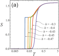
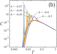
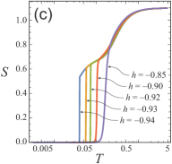
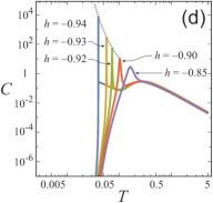
Figure 3: The entropy and specific heat of the $qFM_{1}$ states near the $FR_{2}$-$FM_{1}$ boundary (a, b) with $q=5$, $J=-0.5$, $K=1$, and (c, d) with $q=3$, $J=-0.05$, $K=1$, in an external field $h$. The dotted lines in (b) and (d) show the magnitude of $C_{p}$ at $T=T_{p}$ given by equations (37) and (39) respectively.

The entropy and specific heat of the $qFM_{1}$ states having $q=5$, $J=-0.5$, $K=1$ in a given external field $h$ are shown in Fig. 3a,b. At sufficiently low temperatures, the $qFR_{2}$-$qFM_{1}$ pseudo-transition is observed, which is accompanied by a jump in entropy and a narrow peak in the specific heat.

For the $qFR_{2}$-$qFM_{1}$ transition at $q>3$, the condition $x_{p}\ll q-2$ is met, since $J<0$ and $|J|/T_{p}\gg 1$, so approximately

$$a=\ln(q-2),\qquad b=2\sqrt{\frac{q-1}{(q-2)x_{p}k_{p}}}.$$ (36)

The entropy jump $\Delta\mathcal{S}_{p}=\ln(q-2)$ equals to the residual entropy of the $qFR_{2}$ phase (see Table 1). An expression for the maximum value of the specific heat,

$$C_{p}=\frac{\ln^{2}(q-2)}{4}\sqrt{\frac{q-2}{q-1}}\,e^{\frac{K-|J|}{2T_{p}}},$$ (37)

shows that $C_{p}$ decreases for the states close to the point $P_{1}$ in Fig. 1c. The magnitudes of the specific heat peaks (37) are shown in Fig. 3b with dotted lines. It is interesting to note, that $C_{p}\Psi_{\tau}=\tfrac{1}{2}\gamma\ln(q-2)={\rm const}(T_{p})$, so, having a finite height, the specific heat peak tends to the delta function near the $FR_{2}$-$FM_{1}$ boundary with the $T_{p}$ lowering.

In Fig. 3c,d the entropy and specific heat of the $qFM_{1}$ states having $q=3$, $J=-0.05$, $K=1$ in a given external field $h$ are shown. The case $q=3$ is special, since the residual entropy of the $FR_{2}$-$FM_{1}$ boundary is a continuous function for both adjacent phases. For the parameter $a$ we obtain

$$a=\left(1-\ln x_{p}\right)x_{p},$$ (38)

so the necessary condition for a pseudo-transition $b/a\propto e^{(3|J|-K)/2T_{p}}\ll T_{p}/|J|$ is met if $K>3|J|$. Since in this case $J<0$, the entropy jump (33) drops with decreasing of $T_{p}$ due to the exponent in $x_{p}=e^{J/T_{p}}$, as can be seen from Fig. 3c. A maximal value of the specific heat in $T_{p}$ approximately has the following form

$$C_{p}=\frac{\left(1-J/T_{p}\right)^{2}}{4\sqrt{2}}\,e^{\frac{K-5|J|}{2T_{p}}}.$$ (39)

From (39) we may conclude that if $K>5|J|$ the pseudo-transition is accompanied with exponentially high peak of the specific heat. From a general point of view, this issue was discussed in detail in [29, *Rojas2020].

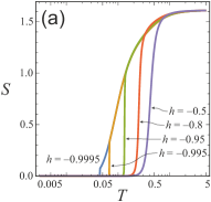
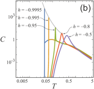
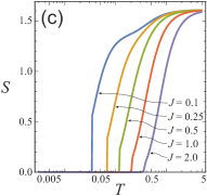
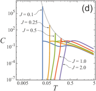
Figure 4: The entropy and specific heat of the $qFM_{1}$ states near the $FM_{1}$-$FM_{2}$ boundary (a, b) with $q=5$, $J=0.25$, $K=1$ in an external field $h$, and (c, d) with $q=5$, $h=-0.995$, $K=1$ for the different values of the coupling parameter $J$. The dotted lines in (b) and (d) show the magnitude of $C_{p}$ at $T=T_{p}$ given by equation (41).

Figure 4 shows the temperature dependencies of the entropy and specific heat for states having parameters close to the $FM_{1}$-$FM_{2}$ boundary for $K=1$. One set of states, shown in Fig. 4a,b, has $J=0.25$ and different values of the external field $h$, and the states in another set, shown in Fig. 4c,d, have the same $h$ and differ in the coupling constant $J$.

Near the $FM_{1}$-$FM_{2}$ boundary, for which the residual entropy is zero, as for both adjacent phases, we get

$$a=(q-2)\frac{1+\ln x_{p}}{x_{p}},\qquad b=\frac{2}{x_{p}}\sqrt{\frac{q-1}{k_{p}}}.$$ (40)

The condition for a pseudo-transition $b/a\propto e^{-K/2T_{p}}\ll T_{p}/|J|$ will met only if $K>0$. In this case $J>0$, so the entropy jump $\Delta\mathcal{S}_{p}=a\propto e^{-J/T_{p}}$ decreases exponentially with decreasing $T_{p}$. This effect is shown in Fig. 4a. The specific heat in $T_{p}$ approximately is given by

$$C_{p}=\frac{(q-2)^{2}\left(1+J/T_{p}\right)^{2}}{4\sqrt{q-1}}\,e^{\frac{K-2J}{2T_{p}}}.$$ (41)

Equation (41) shows that for $K>2J$ the $qFM_{2}$-$qFM_{1}$ pseudo-transition entails an exponentially high peak of the specific heat if the pseudo-transition temperature is small enough. The decrease in the peak of the specific heat near $T_{p}$ with increasing $J$ is shown in Fig. 4d.

III.3 Magnetization and Magnetic susceptibility

It is important to study the magnetization property of the present model. In order to obtain a general average $\langle\delta_{\sigma,\mu}\rangle$, let us define the following operator

$$\bm{m}_{\mu}=\sum_{j=1}^{q}\delta_{j,\mu}|j\rangle\langle j|=|\mu\rangle\langle\mu|.$$ (42)

Therefore, the average of $\bm{m}_{\mu}$ becomes

$$\langle\delta_{\sigma,\mu}\rangle=m_{\mu}=Z_{N}^{-1}\mathop{\mathrm{tr}}\left(\bm{m}_{\mu}\mathbf{V}^{N}\right).$$ (43)

Expressing (42), in eigenstate basis given in (13-15), we have

$$\tilde{\bm{m}}_{\mu}=\sum_{j_{1},j_{2}=1}^{q}\langle u_{j_{1}}|\bm{m}_{\mu}|u_{j_{2}}\rangle|u_{j_{1}}\rangle\langle u_{j_{2}}|,$$ (44)

with

$$\langle u_{j_{1}}|\bm{m}_{\mu}|u_{j_{2}}\rangle=\langle u_{j_{1}}|\mu\rangle\langle\mu|u_{j_{2}}\rangle,$$ (45)

and denoting $\langle\mu|u_{j}\rangle=c_{\mu,j}$, we can write (44) as

$$\tilde{\bm{m}}_{\mu}=\sum_{j_{1},j_{2}=1}^{q}c_{\mu,j_{1}}^{*}c_{\mu,j_{2}}|u_{j_{1}}\rangle\langle u_{j_{2}}|.$$ (46)

In a similar way, the transfer matrix in eigenstate basis (13-15), becomes

$$\tilde{\mathbf{V}}=\sum_{j=1}^{q}\lambda_{j}|u_{j}\rangle\langle u_{j}|.$$ (47)

Hence, substituting (46) and (47) in eq.(43), we obtain

$$m_{\mu}=\frac{1}{Z_{N}}\!\sum_{j_{1}=1}^{q}\langle u_{j_{1}}|\negmedspace\sum_{j_{2},j_{3}=1}^{q}\negmedspace c_{\mu,j_{2}}^{*}c_{\mu,j_{3}}|u_{j_{2}}\rangle\langle u_{j_{3}}|\lambda_{j_{3}}^{N}|u_{j_{1}}\rangle.$$ (48)

In thermodynamic limit ($N\rightarrow\infty$) we can simplify (48). Therefore, writing the magnetization $m_{\mu}$ in terms of $c_{\mu,j}$, it reduces to

$$m_{\mu}=c_{\mu,1}^{*}c_{\mu,1}=|c_{\mu,1}|^{2}.$$ (49)

The explicit expression of coefficients are given by

$$c_{1,1}=\cos\phi,\quad c_{\mu,1}=\frac{\sin\phi}{\sqrt{q-1}},$$ (50)

$$c_{1,2}=\sin\phi,\quad c_{\mu,2}=\frac{\cos\phi}{\sqrt{q-1}},$$ (51)

where $\mu=\{2,\dots,q\}$.

Analogously the remaining coefficients are written by

$$c_{\mu,j}= \begin{cases}0;&\mu=\{1,j+1,\dots,q\}\\ \frac{1}{\sqrt{(j-1)(j-2)}};&\mu=\{2,\dots,j-1\}\\ \sqrt{\frac{j-1}{j-2}};&\mu=j\end{cases},$$ (52)

where we consider $j=\{3,\cdots,q\}$.

As a consequence, we can get the magnetization by using (50) in (49), which becomes

$$m_{1}=\cos^{2}\phi,\quad m_{\mu}=\frac{\sin^{2}\phi}{q-1}.$$ (53)

Additionally, from above result, we get the following identity

$$m_{1}+(q-1)m_{\mu}=1,\quad\mu=\{2,\dots,q\}.$$ (54)

Alternatively one can obtain $m_{1}$ taking the derivative of free energy with respect to external field $h$,

$$m_{1} = \left\langle\delta_{\sigma,1}\right\rangle=-\frac{\partial f}{\partial h},$$ (55)

and $m_{\mu}$ we can obtain from (54).

On the other hand, the magnetic susceptibility $\chi_{1}$ can be obtained deriving (55), which results in

$$\chi_{1}=\frac{1}{4T}\sin(2\phi)^{3}\left(\frac{d_{1}+d_{2}+(q-2)t_{2}}{2t_{1}\sqrt{q-1}}\right),$$ (56)

Similarly, one can obtain for $\mu=\{2,\dots,q\}$,

$$\chi_{\mu}=\frac{\partial m_{\mu}}{\partial h},$$ (57)

and we have the following relation

$$\chi_{\mu}=-\frac{1}{q-2}\chi_{1},$$ (58)

for $\mu=\{2,\dots,q\}$.

To find an approximate expression for the magnetization near $T_{p}$, we can write it by using equations (17) and (55) in the form

$$m_{1}=\frac{T}{\lambda_{1}}\frac{\partial\lambda_{1}}{\partial h}.$$ (59)

When calculating the derivative with respect to $h$, we take into account that $\tfrac{\partial}{\partial h}w_{1}=\beta w_{1}$, $\tfrac{\partial}{\partial h}w_{-1}=0$, $\tfrac{\partial}{\partial h}w_{0}^{2}=\beta w_{0}^{2}$, and obtain

$$m_{1}=\frac{1}{2\lambda_{1}}\left(w_{1}+\frac{(w_{1}-w_{-1})w_{1}+2w_{0}^{2}}{(w_{1}-w_{-1})^{2}+4w_{0}^{2}}\right).$$ (60)

Using equations (24-29) and leaving only the leading terms, we find an approximation for $m_{1}$ in the following form:

$$m_{1}\approx\frac{1}{2}\left(1-\frac{a\tau}{\sqrt{a^{2}\tau^{2}+b^{2}}}\right).$$ (61)

Equation (61) describes the jump in magnetization from $m_{1}=0$ at $\tau>b/a$ to $m_{1}=1$ at $\tau<-b/a$ in the small vicinity of $T_{p}$ for both $qFR_{2}$-$qFM_{1}$ and $qFM_{2}$-$qFM_{1}$ pseudo-transitions.

Similarly, for the susceptibility $\chi_{1}$ we may write, differentiating (59) with respect to $h$:

$$\chi_{1}=-\frac{m_{1}^{2}}{T}+\frac{T}{\lambda_{1}}\frac{\partial^{2}\lambda_{1}}{\partial h^{2}}.$$ (62)

The quasi-singular behavior in $T_{p}$ is caused by the second term in (62). Using the same steps as in deriving (61) and leaving the main contributions, we come to the following approximations for the susceptibility near $T_{p}$:

$$\chi_{1}\approx\frac{b^{2}}{2T_{p}\left(a^{2}\tau^{2}+b^{2}\right)^{\frac{3}{2}}},$$ (63)

and its maximum value:

$$\chi_{1,p}=\frac{b^{-1}}{2T_{p}}.$$ (64)

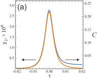
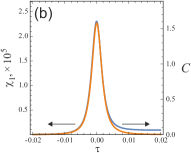
Figure 5: The specific heat (blue line) and susceptibility (orange line) peaks in the vicinity of pseudo-transition points at (a) $q=3$, $J=-0.25$, $K=1$, $h=-0.749995$, and (b) $q=5$, $J=1$, $K=1$, $h=-0.9999$.

Comparing (34) and (63), we see that dependencies of the specific heat and susceptibility in the vicinity of $T_{p}$ are similar: they have the same half-width at half-maximum $\Psi_{\tau}$ and differ by a scale factor $\alpha$, which is the ratio of the specific heat and susceptibility in the pseudo-transition point

$$\alpha=\frac{C_{p}}{\chi_{1,p}}=a^{2}T_{p}.$$ (65)

If for the $qFR_{2}$-$qFM_{1}$ pseudo-transition at $q>3$ the factor $\alpha$ decreases linearly with lowering $T_{p}$, for the $qFR_{2}$-$qFM_{1}$ pseudo-transition at $q=3$ and the $qFM_{2}$-$qFM_{1}$ pseudo-transition, it decreases exponentially due to dependence of $a$. In both the latter cases, for some parameters, the giant magnitude of $\chi_{1,p}$ can be realized at the low magnitude of $C_{p}$. Indeed, for the $qFR_{2}$-$qFM_{1}$ pseudo-transition at $q=3$, we have $\chi_{1,p}\propto e^{(K-|J|)/2T_{p}}$, so the giant peak of susceptibility exists at sufficiently low $T_{p}$ in the entire pseudo-transition region defined, as it was found earlier (see equation (38)), by the condition $K>3|J|$, but for the specific heat it becomes exponentially high only if $K>5|J|$ due to equation (39). This case is shown in Fig. 5a, where in the vicinity of the $qFR_{2}$-$qFM_{1}$ pseudo-transition at $q=3$, $J=-0.25$, $K=1$, the peaks of the specific heat and susceptibility differ in amplitude by seven orders of magnitude and coincide in shape. In turn, for the $qFM_{2}$-$qFM_{1}$ pseudo-transition we have $\chi_{1,p}\propto e^{(K+2J)/2T_{p}}$. Taking into account (40), we can conclude that the giant peak of susceptibility exists for all $J>0$ at $K>0$, while for the specific heat, the giant peak exists only at $0<2J<K$, as it follows from equation (41). The similarity of the specific heat and susceptibility peaks in the vicinity of the $qFM_{2}$-$qFM_{1}$ pseudo-transition at $q=5$, $J=1$, $K=1$, is shown in Fig. 5b.

Temperature dependencies of the magnetic moment and susceptibility of the $qFM_{1}$ states near the $FR_{2}$-$FM_{1}$ boundary are shown in Fig. 6. These states both for $q=5$, $J=-0.5$ and $q=3$, $J=-0.05$ exhibit the $qFR_{2}$-$qFM_{1}$ pseudo-transition with the continuous jump in the magnetic moment and the exponentially high peak of susceptibility. Figure 7 shows the magnetic moment and susceptibility for the same set of states as in Fig. 4. The dotted lines in Fig. 6b,d and in Fig. 7b,d show an approximate value of susceptibility in the pseudo-transition point defined by equation (64).

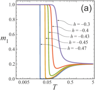
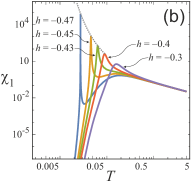
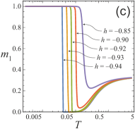
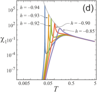
Figure 6: The magnetic moment and susceptibility of the $qFM_{1}$ states near the $FR_{2}$-$FM_{1}$ boundary (a, b) with $q=5$, $J=-0.5$, $K=1$, and (c, d) with $q=3$, $J=-0.05$, $K=1$, in an external field $h$. The dotted lines in (b) and (d) show the magnitude of $\chi_{1,p}$ at $T=T_{p}$ given by equation (64).

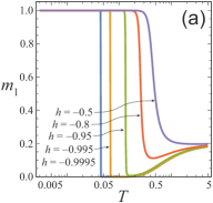
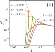
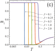
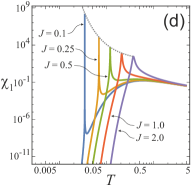
Figure 7: The magnetic moment and susceptibility of the $qFM_{1}$ states near the $FM_{1}$-$FM_{2}$ boundary (a, b) with $q=5$, $J=0.25$, $K=1$ in an external field $h$, and (c, d) with $q=5$, $h=-0.995$, $K=1$ for the different values of the coupling parameter $J$. The dotted lines in (b) and (d) show the magnitude of $\chi_{1,p}$ at $T=T_{p}$ given by equation (64).

Temperature dependencies of the magnetic moment, and susceptibility for states near the $FM_{1}$-$FM_{2}$ boundary at $K=0$ and $K<0$ are shown in Fig. 8. It can be seen the qualitative difference from the case $K>0$. At $K\leq 0$, the magnetic moment changes with decreasing temperature from the value at the $FM_{1}$-$FM_{2}$ boundary, $m_{1}=\tfrac{1}{q-1}$ at $K=0$ or $m_{1}=\tfrac{1}{2}$ at $K<0$, to the values of the magnetic moment in the $FM_{1}$ or $FM_{2}$ phase, which are equal to $1$ and $0$. Because of this, the susceptibility peak is observed in both the $qFM_{1}$ and $qFM_{2}$ states.

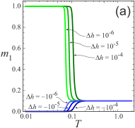
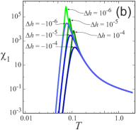
Figure 8: The magnetic moment and susceptibility near the $FM_{1}$-$FM_{2}$ boundary for $qFM_{1}$ and $qFM_{2}$ states (green and blue lines) with $q=10$, $J=1$, (a, b) for $K=0$, in an external field equal to $h=\Delta h$, and (c, d) for $K=-1$, in an external field equal to $h=1+\Delta h$.

As shown if Fig. 8b,d, the peak of susceptibility at $K\leq 0$ becomes arbitrarily large in height for the $qFM_{1}$ and $qFM_{2}$ states, which are quite close to the $FM_{1}$-$FM_{2}$ boundary, but it is significantly wider compared to the case of a pseudo-transition at $K>0$, or near the $qFR_{2}$-$qFM_{1}$ pseudo-transition. The extremely narrow peak, which is characteristic of a pseudo-transition, exists only for $K>0$. This follows formally from equation (40) and the necessary inequality $b/a\ll T_{p}/|J|$. The physical reason for this is the phase separation in the $FM_{1}$-$FM_{2}$ boundary at $K\leq 0$, which causes an intermediate value of the magnetic moment at the $FM_{1}$-$FM_{2}$ boundary and its jump in both the $qFM_{1}$ and $qFM_{2}$ states. The one-dimensional ferromagnetic Ising model has the same properties: zero magnetization of the ground state in the absence of an external field is achieved by splitting into ferromagnetic domains with opposite magnetization, and this state represents the boundary on the phase diagram between phases with magnetizations equal $+1$ and $-1$ depending on the sign of the external field. This situation can be considered as intermediate between microscopic mixing of neighboring phases at the phase boundary when there is no pseudo-transition, and a pure phase equal to one of the neighboring phases when the pseudo-transition is realized.

IV Pair distribution correlation function

In order to accomplish our analysis, we consider the pair distribution correlation function, which is defined as follows

$$\Gamma_{\mu,\mu^{\prime}}^{(r)}=\langle\delta_{\sigma_{i},\mu}\delta_{\sigma_{i+r},\mu^{\prime}}\rangle-\langle\delta_{\sigma_{i},\mu}\rangle\langle\delta_{\sigma_{i+r},\mu^{\prime}}\rangle,$$ (66)

where $\Gamma_{\mu,\mu^{\prime}}^{(r)}\equiv\Gamma_{\mu,\mu^{\prime}}(\sigma_{i},\sigma_{i+r})$.

If the system is translationally invariant, we have $\langle\delta_{\sigma_{i},\mu}\rangle=\langle\delta_{\sigma_{i+r},\mu}\rangle=\langle\delta_{\sigma,\mu}\rangle=m_{\mu}$, and $\Gamma_{\mu,\mu^{\prime}}^{(r)}$ depends only on the distance $(r)$.

Now let us defined the average of PDF,

$$g_{\mu,\mu^{\prime}}^{(r)}=\langle\delta_{\sigma_{i},\mu}\delta_{\sigma_{i+r},\mu^{\prime}}\rangle=\langle\bm{m}_{\mu}\bm{m}_{\mu^{\prime}}\rangle,$$ (67)

so, in natural basis is expressed by

$$g_{\mu,\mu^{\prime}}^{(r)}=Z_{N}^{-1}\mathop{\mathrm{tr}}\left(\bm{m}_{\mu}\mathbf{V}^{r}\bm{m}_{\mu^{\prime}}\mathbf{V}^{N-r}\right)$$ (68)

whereas in eigenstate basis becomes

$$g_{\mu,\mu^{\prime}}^{(r)}=Z_{N}^{-1}\mathop{\mathrm{tr}}\left(\tilde{\bm{m}}_{\nu}\mathbf{\tilde{V}}^{r}\tilde{\bm{m}}_{\tau}\tilde{\mathbf{V}}^{N-r}\right).$$ (69)

Writing in terms of eigenstates

$$g_{\mu,\mu^{\prime}}^{(r)}= Z_{N}^{-1}\sum_{j_{1}=1}^{q}\langle u_{j_{1}}|\sum_{j_{2},j_{3}=1}^{q}c_{\mu,j_{2}}^{*}c_{\mu,j_{3}}|u_{j_{2}}\rangle\langle u_{j_{3}}|\lambda_{j_{3}}^{r}$$

$$\times\sum_{j_{4},j_{5}=1}^{q}c_{\mu^{\prime},j_{4}}^{*}c_{\mu^{\prime},j_{5}}|u_{j_{4}}\rangle\langle u_{j_{5}}|\lambda_{j_{5}}^{N-r}|u_{j_{1}}\rangle$$ (70)

and simplifying (70), we have

$$g_{\mu,\mu^{\prime}}^{(r)}=Z_{N}^{-1}\sum_{j_{1}=1}^{q}\sum_{j_{2}=1}^{q}c_{\mu,j_{1}}^{*}c_{\mu,j_{2}}\lambda_{j_{2}}^{r}c_{\mu^{\prime},j_{2}}^{*}c_{\mu^{\prime},j_{1}}\lambda_{j_{1}}^{N-r},$$ (71)

in thermodynamic limit $(Z_{N}\rightarrow\lambda_{1}^{N})$. The above expression reduces to

$$g_{\mu,\mu^{\prime}}^{(r)}=\sum_{j_{1}=1}^{q}\sum_{j_{2}=1}^{q}c_{\mu,j_{1}}^{*}c_{\mu,j_{2}}\Bigl{(}\tfrac{\lambda_{j_{2}}}{\lambda_{1}}\Bigr{)}^{r}c_{\mu^{\prime},j_{2}}^{*}c_{\mu^{\prime},j_{1}}\left(\tfrac{\lambda_{j_{1}}}{\lambda_{1}}\right)^{N-r},$$ (72)

manipulating conveniently, we have

$$g_{\mu,\mu^{\prime}}^{(r)}=c_{\mu,1}^{*}c_{\mu,1}c_{\mu^{\prime},1}^{*}c_{\mu^{\prime},1}+\sum_{j=2}^{q}c_{\mu,1}^{*}c_{\mu,j}\Bigl{(}\tfrac{\lambda_{j}}{\lambda_{1}}\Bigr{)}^{r}c_{\mu^{\prime},j}^{*}c_{\mu^{\prime},1},$$ (73)

or even in terms of eq.(43), we have

$$g_{\mu,\mu^{\prime}}^{(r)}=m_{\mu}m_{\mu^{\prime}}+c_{\mu,1}^{*}c_{\mu^{\prime},1}\sum_{j=2}^{q}c_{\mu,j}c_{\mu^{\prime},j}^{*}\Bigl{(}\tfrac{\lambda_{j}}{\lambda_{1}}\Bigr{)}^{r}.$$ (74)

Therefore, we can write the correlation function as follows

$$\Gamma_{\mu,\mu^{\prime}}^{(r)}=c_{\mu,1}^{*}c_{\mu^{\prime},1}\sum_{j=2}^{q}c_{\mu,j}c_{\mu^{\prime},j}^{*}\Bigl{(}\tfrac{\lambda_{j}}{\lambda_{1}}\Bigr{)}^{r}=\\ =c_{\mu,1}^{*}c_{\mu^{\prime},1}\Bigl{\{}c_{\mu,2}c_{\mu^{\prime},2}^{*}\left(\tfrac{\lambda_{2}}{\lambda_{1}}\right)^{r}+\left(\tfrac{\lambda_{3}}{\lambda_{1}}\right)^{r}\sum_{j=3}^{q}c_{\mu,j}c_{\mu^{\prime},j}^{*}\Bigr{\}}.$$ (75)

Note that for $q=2$, the last term in (75) ceases to exist.

Taking into account the orthogonality relations for the coefficients in (13,14,15),

$$\sum_{j=1}^{q}c_{\mu,j}c_{\mu^{\prime},j}^{*}=\delta_{\mu,\mu^{\prime}},$$ (76)

thus (75) becomes

$$\Gamma_{\mu,\mu^{\prime}}^{(r)}=c_{\mu,1}^{*}c_{\mu^{\prime},1}\Bigl{\{}c_{\mu,2}c_{\mu^{\prime},2}^{*}\left(\tfrac{\lambda_{2}}{\lambda_{1}}\right)^{r}+\\ +\left(\delta_{\mu,\mu^{\prime}}-c_{\mu,1}c_{\mu^{\prime},1}^{*}-c_{\mu,2}c_{\mu^{\prime},2}^{*}\right)\left(\tfrac{\lambda_{3}}{\lambda_{1}}\right)^{r}\Bigr{\}}.$$ (77)

From (77), and after some algebraic manipulation, we can find the pair correlation functions in terms of magnetization and transfer matrix eigenvalues, which has the following form

$$\Gamma_{1,1}^{(r)} =m_{1}(1-m_{1})\left(\tfrac{\lambda_{2}}{\lambda_{1}}\right)^{r},$$ (78)

$$\Gamma_{\mu,\mu}^{(r)} =(1-m_{1})\left[m_{1}\left(\tfrac{\lambda_{2}}{\lambda_{1}}\right)^{r}+(q-2)\left(\tfrac{\lambda_{3}}{\lambda_{1}}\right)^{r}\right],$$ (79)

$$\Gamma_{1,\mu}^{(r)} =-\tfrac{m_{1}(1-m_{1})}{q-1}\left(\tfrac{\lambda_{2}}{\lambda_{1}}\right)^{r},$$ (80)

$$\Gamma_{\mu,\mu^{\prime}}^{(r)} =(1-m_{1})\left[m_{1}\left(\tfrac{\lambda_{2}}{\lambda_{1}}\right)^{r}-\left(\tfrac{\lambda_{3}}{\lambda_{1}}\right)^{r}\right],$$ (81)

where $\mu,\mu^{\prime}=2,\ldots q$ and $\mu\neq\mu^{\prime}$. An alternative expression of eqs.(78-81) are given in appendix A.

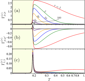
Figure 9: The pair distribution correlation function $\Gamma_{\mu,\mu^{\prime}}^{(r)}$ as a function of temperature $T$ in logarithmic scale, assuming fixed $q=5$, $J=0.9$, $K=1$, $h=-0.995$ and several values of $r$. (a) For $\mu=\mu^{\prime}$, with $\mu=\{2,3,\dots\}$. (b) For $\mu\neq\mu^{\prime}$ with $\mu,\mu^{\prime}=\{2,3,\dots\}$. (c) For $\mu=\mu^{\prime}=1$.

In Fig. 9 we illustrate the pair correlation function $\Gamma_{\mu,\mu^{\prime}}^{(r)}$ as a function of temperature in logarithmic scale, here we consider the following fixed parameters $q=5$, $J=0.9$, $K=1$, $h=-0.995$ and several distances $r=\{1,5,10,20,50,100\}$. In panel (a) we report for the case of $\mu=\mu^{\prime}$ and $\mu=\{2,3,\dots\}$, given by eq.(79). It is worth notice that for $T<T_{p}$ (enough below) this amount is closely null, meaning that the pair distribution spins orientations have no almost relationship, although for $T>T_{p}$ (enough above) the system exhibits clearly the relationship between pair spins orientations and as expected decreases with the distances as well as temperature. In panel (b) is depicted the correlation function for the case $\mu\neq\mu^{\prime}$ and $\mu,\mu^{\prime}=\{2,3,4,\dots\}$, given by eq.(81). For $T<T_{p}$ (enough below) the $\Gamma_{\mu,\mu^{\prime}}^{(r)}$ become nearly null correlation function, while for $T>T_{p}$ (enough above) the systems exhibits a qualitatively different behavior, which in module decreases with with $r$ and $T$. In panel (c) is displayed for the case of $\mu=\mu^{\prime}=1$ (according eq.(78)), for this particular case we observe that the correlation function becomes almost null far enough from the pseudo-critical temperature $T_{p}$, while at $T_{p}$ the correlation function illustrate a peak, which decreases as expected with $r$. The case $\mu=1$ and $\mu^{\prime}=\{2,3,\dots\}$ given by eq.(81) is simply the same to the case eq.(78) divided by $(q-1)$.

We can also notice that the four expression given by (78-81) satisfy the following couple of identities

$$\Gamma_{1,1}^{(r)}+(q-1)\Gamma_{1,\mu}^{(r)}= 0,$$ (82)

$$\Gamma_{\mu,\mu}^{(r)}+\Gamma_{1,\mu}^{(r)}+(q-2)\Gamma_{\mu,\mu^{\prime}}^{(r)}= 0.$$ (83)

An equivalent expressions of the relations (82-83) are given in appendix A.

Similarly, we can obtain a couple of identities for $g$’s, by using (82) and (83) which reduce to the following relations

$$g_{1,1}^{(r)}+\left(q-1\right)g_{1,\mu}^{(r)}= m_{1},$$ (84)

$$g_{\mu,\mu}^{(r)}+g_{1,\mu}^{(r)}+(q-2)g_{\mu,\mu^{\prime}}^{(r)}= m_{\mu},$$ (85)

which is useful to studying the phase diagram, like illustrated in Table 1.

Table 1: The nearest neighbour pair distribution functions $g_{\mu,\mu^{\prime}}^{(1)}$, $\mu,\mu^{\prime}=2,\ldots q$, magnetization $m_{1}$, and entropy $\mathcal{S}$ of the frustrated Potts chain at zero temperature. Here $q_{1}=\sqrt{4q-3}$, $q_{2}=\sqrt{(q-1)(q+3)}$, $q_{3}=1+\sqrt{q-1}$, and $q_{4}=\sqrt{(q-1)^{2}+4}$.

GS phase	$g_{1,1}^{(1)}$	$g_{\mu,\mu}^{(1)}$	$g_{1,\mu}^{(1)}$	$g_{\mu,\mu^{\prime}}^{(1)}$	$m_{1}$	$\mathcal{S}$
$FM_{1}$	$1$	$0$	$0$	$0$	$1$	$0$
$FM_{2}$	$0$	$\dfrac{1}{q-1}$	$0$	$0$	$0$	$0$
$FR_{1}$	$0$	$0$	$\dfrac{1}{2\left(q-1\right)}$	$0$	$\dfrac{1}{2}$	$\frac{1}{2}\ln\left(q-1\right)$
$FR_{2}$	$0$	$0$	$0$	$\dfrac{1}{\left(q-1\right)\left(q-2\right)}$	0	$\ln\left(q-2\right)$
$FR_{1}$-$FM_{1}$	$\dfrac{1}{q_{1}}$	$0$	$\dfrac{q_{1}-1}{2q_{1}\left(q-1\right)}$	$0$	$\dfrac{2q-1+q_{1}}{q_{1}\left(1+q_{1}\right)}$	$\ln\dfrac{1+q_{1}}{2}$
$FR_{2}$-$FM_{2}$	$0$	$\dfrac{1}{\left(q-1\right)^{2}}$	$0$	$\dfrac{1}{\left(q-1\right)^{2}}$	$0$	$\ln\left(q-1\right)$
$FR_{1}$-$FR_{2}$	$0$	$0$	$\dfrac{1}{q\left(q-1\right)}$	$\dfrac{1}{q\left(q-1\right)}$	$\dfrac{1}{q}$	$\ln\left(q-1\right)$
$FR_{1}$-$FM_{2}$ ($K<0$)	$0$	$\dfrac{1}{q_{1}\left(q-1\right)}$	$\dfrac{q_{1}-1}{2q_{1}\left(q-1\right)}$	$0$	$\dfrac{2q-2}{q_{1}\left(1+q_{1}\right)}$	$\ln\dfrac{1+q_{1}}{2}$
$FR_{2}$-$FM_{1}$ ($K>0$)	$0$	$0$	$0$	$\dfrac{1}{\left(q-1\right)\left(q-2\right)}$	$0$	$\ln\left(q-2\right)$
$FM_{1}$-$FM_{2}$ ($K>0$)	$0$	$\dfrac{1}{q-1}$	$0$	$0$	$0$	$0$
$FM_{1}$-$FM_{2}$ ($K=0$)	$\dfrac{1}{q}$	$\dfrac{1}{q}$	$0$	$0$	$\dfrac{1}{q}$	$0$
$FM_{1}$-$FM_{2}$ ($K<0$)	$\dfrac{1}{2}$	$\dfrac{1}{2\left(q-1\right)}$	$0$	$0$	$\dfrac{1}{2}$	$0$
$Q_{1}$	$0$	$\dfrac{1}{q_{2}\left(q-1\right)}$	$\dfrac{2}{q_{2}\left(q-1+q_{2}\right)}$	$\dfrac{1}{q_{2}\left(q-1\right)}$	$\dfrac{2}{q+3+q_{2}}$	$\ln\dfrac{q-1+q_{2}}{2}$
$Q_{2}$	$\dfrac{1}{2q_{3}}$	$\dfrac{1}{2q_{3}\left(q-1\right)}$	$\dfrac{1}{2q_{3}\sqrt{q-1}}$	$0$	$\dfrac{1}{2}$	$\ln q_{3}$
$P_{1}$	$\dfrac{3-q+q_{4}}{q_{4}\left(q-1+q_{4}\right)}$	$0$	$\dfrac{2}{q_{4}\left(q-1+q_{4}\right)}$	$\dfrac{q-3+q_{4}}{q_{4}\left(q-1\right)\left(q-1+q_{4}\right)}$	$\dfrac{q+1+q_{4}}{q_{4}\left(q-1+q_{4}\right)}$	$\ln\dfrac{q-1+q_{4}}{2}$
$P_{2}$	$0$	$\dfrac{1}{\left(q-1\right)^{2}}$	$0$	$\dfrac{1}{\left(q-1\right)^{2}}$	$0$	$\ln\left(q-1\right)$
$S$	$\dfrac{1}{q^{2}}$	$\dfrac{1}{q^{2}}$	$\dfrac{1}{q^{2}}$	$\dfrac{1}{q^{2}}$	$\dfrac{1}{q}$	$\ln q$

IV.1 Correlation length

From transfer matrix eigenvalues, one can observe that $1>\tfrac{\lambda_{2}}{\lambda_{1}}>\tfrac{\lambda_{3}}{\lambda_{1}}$, thus for $r>1$, we can ignore $\left(\tfrac{\lambda_{3}}{\lambda_{1}}\right)^{r}\rightarrow 0$, since $\left(\tfrac{\lambda_{2}}{\lambda_{1}}\right)^{r}\gg\left(\tfrac{\lambda_{3}}{\lambda_{1}}\right)^{r}$. Consequently, we can define the correlation length as follows

$$\xi=\left[\ln\left(\frac{\lambda_{1}}{\lambda_{2}}\right)\right]^{-1}.$$ (86)

An approximation for the correlation length in the vicinity of the pseudo-transition point immediately follows from equations (30) for the eigenvalues:

$$\xi\approx\frac{1}{\sqrt{a^{2}\tau^{2}+b^{2}}}.$$ (87)

At the pseudo-transition point the correlation length reaches extremely high values

$$\xi_{p}=b^{-1},$$ (88)

since the condition $b\ll 1$ is necessarily satisfied. Indeed, using the expressions of $b$ in the given limit cases, we obtain

$$\xi_{p}=\left\{\begin{array}[]{ll}\tfrac{1}{2}\sqrt{\tfrac{(q-2)x_{p}k_{p}}{q-1}}\propto e^{\frac{K-|J|}{2T_{p}}},&qFR_{2}{-}qFM_{1};\\[10.00002pt] \tfrac{x_{p}}{2}\sqrt{\tfrac{k_{p}}{q-1}}\propto e^{\frac{K+2J}{2T_{p}}},&qFM_{2}{-}qFM_{1}.\end{array}\right.$$ (89)

The half-width at half-maximum for the peak (87) of the correlation length is $\tilde{\Psi}_{\tau}=\sqrt{3}b/a$ and only by numeric factor differs from $\Psi_{\tau}$.

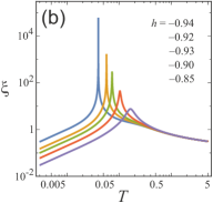
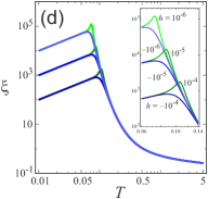
Figure 10: The correlation length for $qFM_{1}$ states with (a) $q=5$, $J=-0.5$, $K=1$, (b) $q=3$, $J=-0.05$, $K=1$, (c) $q=5$, $J=0.25$, $K=1$, and for (d) $qFM_{1}$ and $qFM_{2}$ states with $q=10$, $J=1$, $K=0$, at a given $h$.

Figure 10 shows the temperature dependences of the correlation length for the same sets of states as in Fig. 6b, 6d, 7b, and 8b. As for the specific heat and susceptibility, the correlation length near the pseudo-transition point in Fig. 10a,b,c shows the giants peaks, which are qualitatively different from other cases like shown in Fig. 10d.

V Pseudo-critical exponents

Now let us analyze the nature of the peaks of the specific heat, susceptibility, and correlation length around $T_{p}$, whether follow some critical exponent universality. A general technique to calculate the critical exponents in the systems that exhibit was developed in Ref. [31]. For the one-dimensional frustrated $q$-state Potts model, we can find these quantities directly from approximations (34), (63), and (87). Considering the region of $\tau$ where the curvature of the peaks becomes positive, $b/a<|\tau|\ll T_{p}/|J|$, we obtain the following asymptotics

$$\xi= \;c_{\xi}|\tau|^{-1}, \qquad c_{\xi}=a^{-1},$$ (90)

$$C= \;c_{f}|\tau|^{-3}, \qquad c_{f}=\frac{1}{2}a^{-1}b^{2},$$ (91)

$$\chi_{1}= \;c_{\chi}|\tau|^{-3}, \qquad c_{\chi}=\frac{1}{2T_{p}}a^{-3}b^{2}.$$ (92)

These found critical exponents are the same as for one-dimensional models of the general class with pseudo-transitions [31]. Combining the critical amplitudes, one can write the following relation

$$\frac{c_{f}}{c_{\chi}}\,c_{\xi}^{2}=T_{p},$$ (93)

which is fulfilled for all pseudo-transitions in the frustrated Potts model.

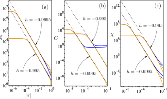
Figure 11: (a) The correlation as a function of $|\tau|$ in logarithmic scale, for $q=5$, $J=0.25$, $K=1$, blue curves correspond to $\tau>0$, orange curves denote the case $\tau<0$, and dotted lines correspond to $\xi(\tau)$ in asymptotic limit. (b) The specific heat as a function of $|\tau|$ in logarithmic scale for the same set of fixed parameters in (a). (c) The magnetic susceptibility as a function of $|\tau|$ in logarithmic scale, for the parameters assumed in panel (a).

In Fig. 11 we verify the power law behavior around the peak for some physical quantities, these results are only valid for the ascending and descending part of the peak, while this approach fails around the top of the peak. In panel (a) we report the correlation length as a function of $|\tau|$ in logarithmic scale assuming the parameters $q=5$, $J=0.25$, $K=1$. Blue curves correspond for $\tau>0$, orange curves denote for $\tau<0$, and dotted lines describe the asymptotic behavior given by eq. (90). We consider two values of the magnetic field as indicated in Fig. 11a. For $h=-0.995$, we can observe clearly a straight line with pseudo-critical exponent $\nu=1$ in a range of $10^{-4}\lesssim\tau\lesssim 10^{-1}$ (blue curve). Suchlike behavior we also observe for the case $-10^{-1}\lesssim\tau\lesssim-10^{-4}$ (orange curve). Note that for $|\tau|\lesssim 10^{-4}$ the asymptotic behavior fails because it corresponds to the peak of the curve. Similar behavior is illustrated for $h=-0.9995$ the pseudo-critical exponent is accurately described by a straight line with the same exponent $\nu=1$. Although the asymptotic approach is valid roughly in the interval $10^{-1}\lesssim|\tau|\lesssim 10^{-6}$. In panel (b) is depicted the specific heat as a function of $|\tau|$ in logarithmic scale, assuming the same fixed parameters to that considered in panel (a), the specific heat also exhibits in the ascending a descending part of the peak as a straight line, which fits precisely to a straight dotted line with angular coefficient $\alpha=3$ given by eq. (91), although evidenced in the shorter interval and for smaller $|\tau|$, the straight lines fail for $|\tau|\lesssim 10^{-5}$ ($h=-0.9995$) and $|\tau|\lesssim 5\cdot 10^{-3}$ ($h=-0.995$), because we are dealing with a peak and not a real singularity. Analogous behavior is observed for the magnetic susceptibility in panel (c), assuming the same set of fixed parameters given in panel (a). Once again, we observe clearly a straight line with angular coefficient $\mu=3$ given by eq. (92), which is valid for a wider interval compared to that of specific heat.

In summary, the pseudo-critical exponents are independent of the magnetic field. We also conclude that these exponents satisfy the same universality class found previously for other one-dimensional models.

VI Conclusion

Although one-dimensional systems could appear thoroughly studied, they still surprise us by exhibiting unconventional new physics. There are some peculiar one-dimensional models, that exhibit the presence of phase transition at finite temperature, under the condition of nearest neighbor interaction[21, 22, *galisova20, 24, 25, 26, 27]. One-dimensional models of statistical physics are attractive from both theoretical and experimental points of view, often driven to develop new methods in order to solve more realistic models.

Here we investigated more carefully the one-dimensional Potts model with an external magnetic field and anisotropic interaction that selects neighboring sites that are in the spin state 1, by using the transfer matrix method. The largest and the second largest eigenvalues are almost degenerate for a given temperature, leading to the arising of pseudo-transition. The rise of anomalous behavior in this model lies in the peculiar behavior of the transfer matrix elements, all transfer matrix elements are positive, but some off-diagonal matrix in the low-temperature region can be extremely small compared to at least two diagonal elements. We have analyzed, the present model for several physical quantities assuming $K=1$. The entropy and magnetization show a steep function around pseudo-critical temperature, rather similar to a first-order phase transition, while the correlation length, specific heat, and magnetic susceptibility exhibit sharp peaks, around pseudo-critical temperature, resembling a second-order phase transition, albeit there is no true divergence. A further investigation of the pseudo-critical exponent satisfy the same class of universality previously identified for other one-dimensional models, these exponents are: for correlation length $\nu=1$, specific heat $\alpha=3$ and magnetic susceptibility $\mu=3$. Whereas for $K=0$ (standard Potts chain), we observe a qualitatively different behavior, such as in entropy there is no step-like function, there is no sharp peak in specific heat, while broad peak arises for magnetic susceptibility.

It is worthy to mention that the pseudo-transition is quite different from that true phase transition because there is no jump in the first derivative of free energy, nor divergence in the second derivative of free energy. In this sense, it would be fairly relevant to observe this anomalous property experimentally in chemical compounds.

Appendix A Some addition relations

Here we give some additional alternative expressions, which would be useful for further analysis, thus the eqs. (78-81) can be reduced to

$$\Gamma_{1,1}^{(r)} =\tfrac{\sin^{2}(2\phi)}{4}\left(\tfrac{\lambda_{2}}{\lambda_{1}}\right)^{r},$$ (94)

$$\Gamma_{\mu,\mu}^{(r)} =\tfrac{\Gamma_{1,1}^{(r)}}{(q-1)^{2}}+\tfrac{(q-2)\sin^{2}(\phi)}{(q-1)^{2}}\left(\tfrac{\lambda_{3}}{\lambda_{1}}\right)^{r},$$ (95)

$$\Gamma_{1,\mu}^{(r)} =-\tfrac{\Gamma_{1,1}^{(r)}}{q-1},$$ (96)

$$\Gamma_{\mu,\mu^{\prime}}^{(r)} =\tfrac{\Gamma_{1,1}^{(r)}}{(q-1)^{2}}-\tfrac{\sin^{2}(\phi)}{(q-1)^{2}}\left(\tfrac{\lambda_{3}}{\lambda_{1}}\right)^{r}.$$ (97)

Considering the identities given by (82) and (83), we obtain the following identity which must satisfy:

$$\Gamma_{1,1}^{(r)}+\left(q-1\right)\Gamma_{\mu,\mu}^{(r)}+2\left(q-1\right)\Gamma_{1,\mu}^{(r)}+{}\\ +\left(q-1\right)\left(q-2\right)\Gamma_{\mu,\mu^{\prime}}^{(r)}=0.$$ (98)

An equivalent relation we can verify, so the pair average distribution functions obey the identity

$$g_{1,1}^{(r)}+\left(q-1\right)g_{\mu,\mu}^{(r)}+2\left(q-1\right)g_{1,\mu}^{(r)}+{}\\ +\left(q-1\right)\left(q-2\right)g_{\mu,\mu^{\prime}}^{(r)}=1.$$ (99)

Below we simplify for the nearest neighbors PDF $g_{\mu,\mu^{\prime}}^{(1)}$, which can be written as

$$g_{1,1}^{(1)} =\tfrac{\left(\lambda_{1}-\lambda_{3}-(q-1)t_{2}\right)\left(\lambda_{1}+\lambda_{2}-\lambda_{3}-(q-1)t_{2}\right)}{\lambda_{1}\left(\lambda_{1}-\lambda_{2}\right)},$$ (100)

$$g_{\mu,\mu}^{(1)} =\tfrac{\left(\lambda_{3}+t_{2}\right)\left(\lambda_{3}-\lambda_{2}+(q-1)t_{2}\right)}{\left(q-1\right)\lambda_{1}\left(\lambda_{1}-\lambda_{2}\right)},$$ (101)

$$g_{1,\mu}^{(1)} =\tfrac{\left(\lambda_{1}-\lambda_{3}-(q-1)t_{2}\right)\left(\lambda_{3}-\lambda_{2}+(q-1)t_{2}\right)}{\left(q-1\right)\lambda_{1}\left(\lambda_{1}-\lambda_{2}\right)},$$ (102)

$$g_{\mu,\mu^{\prime}}^{(1)} =\tfrac{\left(\lambda_{3}-\lambda_{2}+(q-1)t_{2}\right)t_{2}}{\left(q-1\right)\lambda_{1}\left(\lambda_{1}-\lambda_{2}\right)},$$ (103)

where $\mu,\mu^{\prime}=2,\ldots q$, and $\mu\neq\mu^{\prime}$. This amounts are useful to analysis the phase boundary properties illustrated in Table 1.

References

- Baxter [1982] R. J. Baxter, Exactly solved models in statistical mechanics (Academic Press, London ; New York, 1982).
- Ghulghazaryan et al. [2007] R. G. Ghulghazaryan, K. G. Sargsyan, and N. S. Ananikian, Partition function zeros of the one-dimensional Blume-Capel model in transfer matrix formalism, Physical Review E 76, 021104 (2007).
- Hovhannisyan et al. [2009] V. Hovhannisyan, R. Ghulghazaryan, and N. Ananikian, The partition function zeros of the anisotropic Ising model with multisite interactions on a zigzag ladder, Physica A: Statistical Mechanics and its Applications 388, 1479 (2009).
- van Hove [1950] L. van Hove, Sur L’intégrale de Configuration Pour Les Systèmes De Particules À Une Dimension, Physica 16, 137 (1950).
- Ninio [1976] F. Ninio, A simple proof of the Perron-Frobenius theorem for positive symmetric matrices, Journal of Physics A: Mathematical and General 9, 1281 (1976).
- Cuesta and Sánchez [2004] J. A. Cuesta and A. Sánchez, General Non-Existence Theorem for Phase Transitions in One-Dimensional Systems with Short Range Interactions, and Physical Examples of Such Transitions, Journal of Statistical Physics 115, 869 (2004).
- Kittel [1969] C. Kittel, Phase Transition of a Molecular Zipper, American Journal of Physics 37, 917 (1969).
- Chui and Weeks [1981] S. T. Chui and J. D. Weeks, Pinning and roughening of one-dimensional models of interfaces and steps, Physical Review B 23, 2438 (1981).
- Dauxois and Peyrard [1995] T. Dauxois and M. Peyrard, Entropy-driven transition in a one-dimensional system, Physical Review E 51, 4027 (1995).
- Sarkanych et al. [2017] P. Sarkanych, Y. Holovatch, and R. Kenna, Exact solution of a classical short-range spin model with a phase transition in one dimension: The Potts model with invisible states, Physics Letters A 381, 3589 (2017).
- Zimm and Bragg [1959] B. H. Zimm and J. K. Bragg, Theory of the Phase Transition between Helix and Random Coil in Polypeptide Chains, The Journal of Chemical Physics 31, 526 (1959).
- Badasyan et al. [2010] A. V. Badasyan, A. Giacometti, Y. S. Mamasakhlisov, V. F. Morozov, and A. S. Benight, Microscopic formulation of the Zimm-Bragg model for the helix-coil transition, Physical Review E 81, 021921 (2010).
- Ananikyan et al. [1990] N. S. Ananikyan, S. A. Hajryan, E. S. Mamasakhlisov, and V. F. Morozov, Helix-Coil transition in polypeptides: A microscopical approach, Biopolymers 30, 357 (1990).
- Badasyan et al. [2013] A. Badasyan, A. Giacometti, R. Podgornik, Y. Mamasakhlisov, and V. Morozov, Helix-coil transition in terms of Potts-like spins, The European Physical Journal E 36, 46 (2013).
- Tonoyan et al. [2020] S. Tonoyan, D. Khechoyan, Y. Mamasakhlisov, and A. Badasyan, Statistical mechanics of DNA-nanotube adsorption, Physical Review E 101, 062422 (2020).
- Wu [1982] F. Y. Wu, The Potts model, Reviews of Modern Physics 54, 235 (1982).
- Aharony and Pfeuty [1979] A. Aharony and P. Pfeuty, Dilute spin glasses at zero temperature and the / -state Potts model, Journal of Physics C: Solid State Physics 12, L125 (1979).
- Lubensky and Isaacson [1978] T. C. Lubensky and J. Isaacson, Field Theory for the Statistics of Branched Polymers, Gelation, and Vulcanization, Physical Review Letters 41, 829 (1978).
- Chaves and Riera [1984] C. M. Chaves and R. Riera, Dilute Potts chain in a magnetic field, Canadian Journal of Physics 62, 69 (1984).
- Panov [2020] Y. Panov, Local distributions of the 1D dilute Ising model, Journal of Magnetism and Magnetic Materials 514, 167224 (2020).
- Gálisová and Strečka [2015] L. Gálisová and J. Strečka, Vigorous thermal excitations in a double-tetrahedral chain of localized Ising spins and mobile electrons mimic a temperature-driven first-order phase transition, Physical Review E 91, 022134 (2015).
- Gálisová [2017] L. Gálisová, Magnetization plateau as a result of the uniform and gradual electron doping in a coupled spin-electron double-tetrahedral chain, Physical Review E 96, 052110 (2017).
- Gálisová [2020] L. Gálisová, Pairwise Entanglement in Double-Tetrahedral Chain with Different Landé g-Factors of the Ising and Heisenberg Spins, Acta Physica Polonica A 137, 604 (2020).
- Strečka et al. [2016] J. Strečka, R. C. Alécio, M. L. Lyra, and O. Rojas, Spin frustration of a spin-1/2 Ising–Heisenberg three-leg tube as an indispensable ground for thermal entanglement, Journal of Magnetism and Magnetic Materials 409, 124 (2016).
- Rojas et al. [2016] O. Rojas, J. Strečka, and S. de Souza, Thermal entanglement and sharp specific-heat peak in an exactly solved spin-1/2 Ising-Heisenberg ladder with alternating Ising and Heisenberg inter–leg couplings, Solid State Communications 246, 68 (2016).
- Strečka [2020] J. Strečka, Anomalous Thermodynamic Response in the Vicinity of a Pseudo-Transition of a Spin-1/2 Ising Diamond Chain, Acta Physica Polonica A 137, 610 (2020).
- de Souza and Rojas [2018] S. de Souza and O. Rojas, Quasi-phases and pseudo-transitions in one-dimensional models with nearest neighbor interactions, Solid State Communications 269, 131 (2018).
- Carvalho et al. [2019] I. Carvalho, J. Torrico, S. de Souza, O. Rojas, and O. Derzhko, Correlation functions for a spin- 1 2 Ising-XYZ diamond chain: Further evidence for quasi-phases and pseudo-transitions, Annals of Physics 402, 45 (2019).
- Rojas [2020a] O. Rojas, Residual Entropy and Low Temperature Pseudo-Transition for One-Dimensional Models, Acta Physica Polonica A 137, 933 (2020a).
- Rojas [2020b] O. Rojas, A Conjecture on the Relationship Between Critical Residual Entropy and Finite Temperature Pseudo-transitions of One-dimensional Models, Brazilian Journal of Physics 50, 675 (2020b).
- Rojas et al. [2019] O. Rojas, J. Strečka, M. L. Lyra, and S. M. de Souza, Universality and quasicritical exponents of one-dimensional models displaying a quasitransition at finite temperatures, Physical Review E 99, 042117 (2019).
- Janke and Schakel [2004] W. Janke and A. M. Schakel, Geometrical vs. Fortuin–Kasteleyn clusters in the two-dimensional q-state Potts model, Nuclear Physics B 700, 385 (2004).
- Qian et al. [2005] X. Qian, Y. Deng, and H. W. J. Blöte, Dilute Potts model in two dimensions, Physical Review E 72, 056132 (2005).