A stochastically perturbed fluid-structure interaction problem modeled by a stochastic viscous wave equation

Abstract

We study well-posedness for fluid-structure interaction driven by stochastic forcing. This is of particular interest in real-life applications where forcing and/or data have a strong stochastic component. The prototype model studied here is a stochastic viscous wave equation, which arises in modeling the interaction between Stokes flow and an elastic membrane. To account for stochastic perturbations, the viscous wave equation is perturbed by spacetime white noise scaled by a nonlinear Lipschitz function, which depends on the solution. We prove the existence of a unique function-valued stochastic mild solution to the corresponding Cauchy problem in spatial dimensions one and two. Additionally, we show that up to a modification, the stochastic mild solution is $\alpha$-Hölder continuous for almost every realization of the solution’s sample path, where $\alpha\in[0,1)$ for spatial dimension $n=1$, and $\alpha\in[0,1/2)$ for spatial dimension $n=2$. This result contrasts the known results for the heat and wave equations perturbed by spacetime white noise, including the damped wave equation perturbed by spacetime white noise, for which a function-valued mild solution exists only in spatial dimension one and not higher. Our results show that dissipation due to fluid viscosity, which is in the form of the Dirichlet-to-Neumann operator applied to the time derivative of the membrane displacement, sufficiently regularizes the roughness of white noise in the stochastic viscous wave equation to allow the stochastic mild solution to exist even in dimension two, which is the physical dimension of the problem. To the best of our knowledge, this is the first result on well-posedness for a stochastically perturbed fluid-structure interaction problem.

1 Introduction

We propose a stochastic model for fluid-structure interaction given by a stochastic wave equation augmented by dissipation associated with the effects of an incompressible, viscous fluid:

$$u_{tt}+{2}\mu\sqrt{-\Delta}u_{t}-\Delta u=f(u)W(dt,dx),\qquad\text{ in }\mathbb{R}^{n}.$$ (1)

The wave operator models the elastodynamics of a linearly elastic membrane, where $u$ denotes membrane displacement, while the dissipative part, which is in the form of the Dirichlet-to-Neumann operator applied to the time derivative of displacement, accounts for dissipation due to fluid viscosity, where $\mu$ denotes the fluid viscosity coefficient. The equation is forced by spacetime white noise $W(dt,dx)$, which accounts for stochastic effects in real-life problems. The spacetime white noise is scaled by a nonlinear, Lipschitz function $f(u)$. We show below how this equation is derived from a coupled fluid-structure interaction problem involving the Stokes equations describing the flow of an incompressible, viscous fluid, and the wave equation modeling the elastodynamics of a (stretched) linearly elastic membrane. We consider equation (1) in $\mathbb{R}^{n}$ with $n=1$ and $n=2$, focusing primarily on $n=2$, which is the physical dimension.

We prove the existence of a function-valued mild solution to a Cauchy problem for equation (1), which holds both in dimensions $1$ and $2$. Here, by “mild solution” we refer to a stochastic mild solution defined via stochastic integration involving the Green’s function, specified below in Definition 3.1. This is interesting because our result contrasts the results that hold for the stochastic heat and wave equations: the stochastic heat and the stochastic wave equations do not have function-valued mild solutions in spatial dimension $2$ or higher. Additionally, we prove that sample paths of the stochastic mild solution for the stochastic viscous wave equation are Hölder continuous with Hölder exponents $\alpha\in[0,1)$ for $n=1$, and $\alpha\in[0,1/2)$ for $n=2$.

Our results show that the viscous fluid dissipation in fluid-structure interaction is sufficient to smooth out the rough stochastic nature of the real-life data in the problem modeled by the spacetime white noise. In particular, the Dirichlet-to-Neumann operator controls the high frequencies in the structure (membrane) displacement that are driven by the spacetime white noise. To the best of our knowledge, this is the first result on stochastic fluid-structure interaction.

We begin by describing the fluid-structure interaction model from which the equation (1) arises. Consider a prestressed infinite elastic membrane surface, which is modeled by the linear wave equation

$$u_{tt}-\Delta u=F,\ \ \text{ on }\Gamma:=\{(x_{1},x_{2},0)\in\mathbb{R}^{3}:(x_{1},x_{2})\in\mathbb{R}^{2}\},$$ (2)

where $u(x_{1},x_{2})$ denotes the transverse displacement (in the $x_{3}$ direction) of the elastic surface from its reference configuration $\Gamma$. See Figure 1.

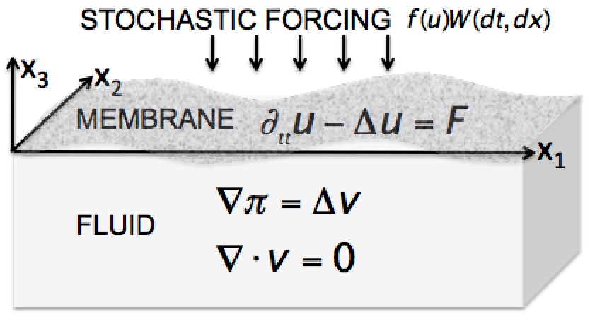
Figure 1: A sketch of the fluid and structure domains.

Beneath this elastic drum surface, we consider a viscous, incompressible fluid, which resides in the lower half-space in $\mathbb{R}^{3}$,

$$\Omega=\{(x_{1},x_{2},x_{3})\in\mathbb{R}^{3}:x_{3}<0\},$$ (3)

modeled by the stationary Stokes equations for an incompressible, viscous fluid:

$$\left.\begin{array}[]{rcl}\nabla\cdot\boldsymbol{\sigma}(\pi,{\boldsymbol{v}})&=&\boldsymbol{0},\\ \nabla\cdot{\boldsymbol{v}}&=&0,\end{array}\right\}\quad{\rm in}\ \Omega=\{(x_{1},x_{2},x_{3})\in{\mathbb{R}}^{3}:x_{3}<0\},$$ (4)

where $\boldsymbol{\sigma}$ is the Cauchy stress tensor, and the unknown quantities are the fluid pressure $\pi:\Omega\to\mathbb{R}$ and the fluid velocity $\boldsymbol{v}:\Omega\to\mathbb{R}^{3}$. We will be assuming that the fluid is Newtonian, so that

$$\boldsymbol{\sigma}=-\pi\boldsymbol{I}+2\mu\boldsymbol{D}(\boldsymbol{v}),$$

where $\mu$ denotes the fluid viscosity coefficient, $\boldsymbol{I}$ is the three by three identity matrix, and $\boldsymbol{D}(\boldsymbol{v})$ is the symmetrized gradient of fluid velocity $\boldsymbol{D}(\boldsymbol{v})=(\nabla\boldsymbol{v}+(\nabla\boldsymbol{v})^{T})/2$. Therefore, the Stokes equations now read

$$\left.\begin{array}[]{rcl}\nabla\pi&=&\mu\triangle\boldsymbol{v},\\ \nabla\cdot{\boldsymbol{v}}&=&0,\end{array}\right\}\quad{\rm in}\ \Omega=\{(x_{1},x_{2},x_{3})\in{\mathbb{R}}^{3}:z<0\},$$ (5)

where we require that the fluid velocity is bounded in the lower half space, and the pressure $\pi\to 0$ as $|x|\to\infty$.

We consider the problem in which the elastic surface is displaced from its reference configuration $\Gamma$ with some given initial displacement and velocity, allowing only vertical displacement, where the elastodynamics of the elastic surface is driven by the total force exerted onto the membrane, which comes from the fluid on one side, and an external stochastic forcing on the other. See Figure 1.

Inifinite domains are considered to simplify the analysis, since the main purpose of this work is to understand the interplay between the dispersion effects in the 2D wave equation, dissipation due to fluid viscosity, and stochasticity imposed by the external forcing, which can be related to the stochasticity of not only the external forcing, but also to the stochasticity of data (e.g., inlet/outlet data) in real-life applications, such as blood flow through arteries.

The fluid and the structure are coupled via two coupling conditions, the kinematic and dynamic coupling conditions, giving rise to the so-called two-way coupled fluid-structure interaction problem. The coupling conditions in the present study are evaluated at a fixed (linearized) fluid-structure interface corresponding to the structure’s reference configuration $\Gamma$. This is known as linear coupling. The two conditions read:

• Kinematic coupling condition. The kinematic coupling condition describes the coupling between the kinematic quantities such as velocity. We will be assuming the no-slip condition, meaning that the fluid and structure velocities are continuous at the interface (there is no slip between the two):

  $$u_{t}=\boldsymbol{v}|_{\Gamma},\ \ {\rm for}\ x=(x_{1},x_{2})\in\mathbb{R}^{2},t\geq 0.$$ (6)

• Dynamic coupling condition. The dynamic coupling condition describes the balance of forces at the fluid-structure interface $\Gamma$, namely, it states that the elastodynamics of the membrane is driven by the force corresponding to the jump in traction (normal stress) across the membrane. On the fluid side, the traction (normal stress) at the interface is given by $-\boldsymbol{\sigma}\boldsymbol{e_{x_{3}}}$, where $\boldsymbol{e_{x_{3}}}$ is the normal vector to $\Gamma$, while on the other side, we are assuming a given loading $F_{ext}(u)$ to be a stochastic process $f(u)W(dt,dx)$ in the $\boldsymbol{e_{x_{3}}}$ direction. Examples of such a loading can be found in cardiovascular applications, see e.g., [30]. Since we assume that the structure only has transversal displacement, the dynamic coupling condition reads:

  $$u_{tt}-\Delta u=-\boldsymbol{\sigma}\boldsymbol{e_{x_{3}}}\cdot\boldsymbol{e_{x_{3}}}+f(u(t,{x}))W(dt,dx)\quad{\rm where}\ x=(x_{1},x_{2})\in\mathbb{R}^{2},t\geq 0.$$ (7)

In fluid-structure interaction problems and physical problems in general, physical phenomena are subject to small random deviations that cause deviations from deterministic behavior. The consideration of such stochastic effects in partial differential equations can give rise to new phenomena, and is an area of active research. Furthermore, in real-life data, one observes such stochastic noise both in terms of the force exerted onto the structure, as well as in the data that drives the problem. For example, the measured inlet/outlet pressure data in a fluid-structure interaction problem describing arterial blood flow, has similar stochastic noise deviations to $F_{ext}(u)=f(u(t,{x}))W(dt,dx)$. Here $W(dt,dx)$ is spacetime white noise in $(t,x)\in\mathbb{R}^{+}\times\mathbb{R}^{2}$, whose properties we will recall in Sec. 2. We will assume that $f:\mathbb{R}\to\mathbb{R}$ is a Lipschitz continuous function. In particular, the case $f\not\equiv 1$ allows dependence of the magnitude of the stochastic noise at each point on the structure displacement $u(t,x)$ itself.

To derive equation (1) as a model which describes the fluid-structure interaction problem (2)-(7), we focus on the dynamic coupling condition (7). The goal is to try to express the effects of fluid normal stress via the Dirichlet-to-Neumann operator defined entirely in terms of $u$ and/or its derivatives. In this derivation we also use the kinematic coupling condition (6) as explained below.

First notice that the right hand-side of (7) is given by

$$-\boldsymbol{\sigma}\boldsymbol{e_{x_{3}}}\cdot\boldsymbol{e_{x_{3}}}=\pi-{2}\mu\frac{\partial v_{x_{3}}}{\partial x_{3}}\ {\rm on}\ \Gamma.$$

Since the tangential displacements are assumed to be zero, the kinematic coupling condition (6) implies that the $x_{1}$ and $x_{2}$ components of the fluid velocity $\boldsymbol{v}$ are zero on $\Gamma$, namely $v_{x_{1}}=v_{x_{2}}=0$ on $\Gamma$. By the divergence free condition, one immediately gets that ${\partial v_{x_{3}}}/{\partial x_{3}}=0$ on $\Gamma$. Therefore,

$$-\boldsymbol{\sigma}\boldsymbol{e_{x_{3}}}\cdot\boldsymbol{e_{x_{3}}}=\pi\quad{\rm on}\ \Gamma,$$ (8)

where $\pi$ is the fluid pressure given as a solution to the Stokes equations (5). So it remains to find an appropriate expression for $\pi$ on $\Gamma$ in terms of the structure displacement $u$. In fact, we will show that the following formula holds

$$\pi=-2\mu\sqrt{-\Delta}u_{t}\quad{\text{on}\ \Gamma},$$ (9)

under the assumption that $u$ and $u_{t}$, along with their spatial derivatives, are smooth functions that are rapidly decreasing at infinity. We will also impose the boundary conditions on (5), stating that the fluid velocity is bounded on the lower half space, and the pressure $\pi$ has a limit equal to zero as $|x|\to\infty$ in the lower half space. Details of this calculation are presented in [25]. Here we present the main steps.

To derive the formula (9), we note that by taking the inner product of the first equation in (5) with $\boldsymbol{e_{x_{3}}}$, we obtain

$$\frac{\partial\pi}{\partial x_{3}}=\mu\Delta_{x_{1},x_{2}}v_{x_{3}}+\mu\frac{\partial^{2}v_{x_{3}}}{\partial x_{3}^{{2}}}=\mu\Delta v_{x_{3}},$$ (10)

where $\Delta_{x_{1},x_{2}}:=\frac{\partial^{2}}{\partial x_{1}^{2}}+\frac{\partial^{2}}{\partial x_{2}^{2}}$. Furthermore, by taking the divergence of the first equation in (5), and by using the divergence-free condition, we get that the pressure $\pi$ is harmonic. Thus, if we can compute the right hand side of (10) on $\Gamma$, we can recover $\pi$ as the solution to a Neumann boundary value problem for Laplace’s equation in the lower half space, with the boundary condition requiring that $\pi$ goes to zero at infinity.

To compute the right hand side of (10), we need to compute $v_{x_{3}}$. Taking the Laplacian on both sides of (10), and using the fact that $\pi$ is harmonic, we obtain

$$\Delta^{2}v_{x_{3}}=0,\qquad\text{ on }\Omega=\{(x_{1},x_{2},x_{3})\in{\mathbb{R}}^{3}:x_{3}<0\}.$$ (11)

Thus, $v_{x_{3}}$ satisfies the biharmonic equation with the following two boundary conditions: from the kinematic coupling condition, we get

$$v_{x_{3}}(x_{1},x_{2},0)=u_{t}(x_{1},x_{2},0),\qquad\text{ on }\Gamma=\{(x_{1},x_{2},x_{3})\in{\mathbb{R}}^{3}:x_{3}=0\},$$ (12)

and from the fact that $v_{x_{1}}=v_{x_{2}}=0$ on $\Gamma$, by the kinematic coupling condition and the fact that $\boldsymbol{v}$ is divergence free, we get

$$\frac{\partial v_{x_{3}}}{\partial x_{3}}(x_{1},x_{2},0)=0,\qquad\text{ on }\Gamma=\{(x_{1},x_{2},x_{3})\in{\mathbb{R}}^{3}:x_{3}=0\}.$$ (13)

We solve (11) with boundary conditions (12) and (13) by taking a Fourier transform in the variables $x_{1}$ and $x_{2}$, but not in $x_{3}$. We will denote the Fourier variables associated with $x_{1}$ and $x_{2}$ by $\xi_{1}$ and $\xi_{2}$, and we will denote ${\xi}=(\xi_{1},\xi_{2})$, $|{\xi}|^{2}=\xi_{1}^{2}+\xi_{2}^{2}$. The Fourier transform equation then reads:

$$|\xi|^{4}\widehat{v_{x_{3}}}({\xi},x_{3})-2|{\xi}|^{2}\frac{\partial^{2}}{\partial x_{3}^{2}}\widehat{v_{x_{3}}}({\xi},x_{3})+\frac{\partial^{4}}{\partial x_{3}^{4}}\widehat{v_{x_{3}}}({\xi},x_{3})=0.$$ (14)

The solution is given by

$$\widehat{v_{x_{3}}}({\xi},x_{3})=\widehat{u_{t}}({\xi})e^{|{\xi}|x_{3}}-|\xi|\widehat{u_{t}}({\xi})x_{3}e^{|{\xi}|x_{3}}.$$ (15)

We can now compute the right hand side of (10). Taking the Fourier transform of (10) in the $x_{1}$ and $x_{2}$ variables, and evaluating the equation on $\Gamma$ by using the kinematic coupling condition (6), we get

$$\frac{\partial\widehat{\pi}}{\partial x_{3}}({\xi},0)=-\mu|\xi|^{2}\widehat{u_{t}}({\xi})+\mu\frac{\partial^{2}\widehat{v_{x_{3}}}}{\partial x_{3}^{{2}}}({\xi},0)=-2\mu|\xi|^{2}\widehat{u_{t}}({\xi}),$$ (16)

where the last equality follows by using the explicit formula for $\widehat{v_{x_{3}}}({\xi},z)$ in (15).

We now know that the pressure $\pi$ is a harmonic function in the lower half space, satisfying the Neumann boundary condition (16) given in Fourier space. To recover formula (9) we want $\pi$ on $\Gamma$. This can be obtained via the Neumann to Dirichlet operator. It is well known that the Dirichlet to Neumann operator for Laplace’s equation in the lower half space is given by $\sqrt{-\Delta}$, thereby having a Fourier multiplier $|\xi|$, see e.g., [4]. Therefore, the Neumann to Dirichlet operator for Laplace’s equation in the lower half space (with the solution to Laplace’s equation having a limit of zero at infinity) is a Fourier multiplier of the form $\frac{1}{|\xi|}$. Thus, the Neumann to Dirichlet operator applied to the Neumann data (16) gives the pressure as Dirichlet data:

$$\widehat{\pi}(\xi)=-2\mu|\xi|\widehat{u_{t}}(\xi)\qquad\text{ on }\Gamma,$$

which establishes the desired formula (9).

The dynamic coupling condition (7), together with (9) gives the stochastic model

$$u_{tt}+\sqrt{-\Delta}u_{t}-\Delta u=f(u)W(ds,dy)\ \ \text{ on }\mathbb{R}^{2},$$

where we have set the fluid viscosity $\mu=1/2$. We will refer to this model as the stochastic viscous wave equation, as it is a stochastic wave equation augmented by the viscous effects of the fluid, which are captured by the Dirichlet to Neumann operator acting on the structure velocity $u_{t}$.

The study of fluid-structure interaction, which concerns the coupled dynamical interactions between fluids and deformable structures/solids, has been the focus of many works. The results related to the analysis of fluid-structure interaction started coming out only within the past 20 years. In particular, fluid-structure interaction problems with linear coupling, which is considered in the current work, have been investigated in, e.g., [1, 2, 15, 27]. The more general case of nonlinear coupling, which has been studied in [3, 5, 6, 7, 9, 10, 16, 17, 18, 20, 21, 26, 28, 29, 31, 32, 33, 34, 35, 36], allows the fluid domain to change as a function of time, and the coupling conditions between the fluid and structure are evaluated at the current location of the interface, not known a priori. This creates additional (geometric) nonlinearities and generates additional mathematical difficulties. In all of these works the focus is on deterministic models, in which there are no stochastic effects.

The study of stochasticity in PDEs has been of recent interest. Most physical phenomena occurring in real-life applications feature the presence of some sort of random noise that perturbs the system from what may be deterministically expected. The types of noise added to the equation can vary, from the simplest spacetime white noise, which intuitively is noise that is “independent at each time and space”, to forms of noise with smoother spatial correlation so that the noise is still independent at separate times, but the noise in space allows for correlation between points and is hence “smoother” than white noise.

Many classical partial differential equations, such as the heat and wave equations, have been studied with the addition of stochastic random forcing. There are many approaches to the study of such stochastic PDEs. One approach uses Walsh’s theory of martingale measures, of which white noise is an example. The theory of integration against such martingale measures can be found in Walsh’s work [39]. Upon defining such an appropriate theory of stochastic integration, one can define what is called a mild solution to a given stochastic partial differential equation by means of the Green’s function.

The choice of the stochastic noise used in the PDE being studied is of utmost importance. White noise, which is noise that is intuitively “independent at all spaces and times”, is a starting point for many studies. In formal mathematical notation, the time and space independence property of white noise is expressed via expectation as

$$\mathbb{E}(\dot{W}(t,x)\dot{W}(s,y))=\delta_{0}(t-s)\delta_{0}(x-y),$$

where $\delta_{0}$ is the Dirac delta function, and $\dot{W}(t,x)$, or $W(dt,dx)$, denotes spacetime white noise. In the rest of this manuscript, we will be using $W(dt,dx)$ to denote spacetime white noise and stochastic integration against white noise.

The white noise perturbed heat and wave equations have interesting properties. When perturbed by white noise, the two equations:

$$u_{t}-\Delta u=W(dx,dt)\quad\text{and}\quad u_{tt}-\Delta u=W(dx,dt)\qquad\text{ in }\mathbb{R}^{n},$$

do not allow function-valued mild solutions in spatial dimensions two and higher, while they do in spatial dimension one. See, for example, [12] and [24], where questions of existence and uniqueness of mild solutions are addressed. This interesting property related to spatial dimensions two and higher is due to the lack of square integrability of the Green’s function in time and space, as we discuss later. Because of this property, “smoother” types of stochastic noise, such as spatially homogeneous Gaussian noise, are used to perturb the stochastic heat and wave equations in higher dimensions in order to yield function-valued mild solutions. In formal mathematical notation, such spatially homogeneous Gaussian noise $\dot{F}(t,x)$ has a covariance structure

$$\mathbb{E}(\dot{F}(t,x)\dot{F}(s,y))=\delta_{0}(t-s)k(x-y),$$ (17)

where $k:\mathbb{R}^{n}\to\mathbb{R}$. Note that the formal case of setting $k$ to be the Dirac delta “function” recovers the previous white noise case, though choosing smoother functions $k$ allows us to formulate “smoother” types of noise. See Sec. 3 of [12] and the work in [13] for more information about spatially homogeneous Gaussian noise. One of the key questions in studying stochastically perturbed PDEs is what conditions on $k$ need to be imposed so that the resulting equation with the spatially homogeneous Gaussian noise with covariance structure (17) has function-valued mild solutions? See, for example [13], and for more general contexts [11] and [22].

In the current manuscript, we do not need the properties of general spatially homogeneous Gaussian noise. This is because, as we shall see below, the viscous wave equation

$$u_{tt}+\sqrt{-\Delta}u_{t}-\Delta u=F,\qquad\text{ on }\mathbb{R}^{n},$$ (18)

first considered in [25] as a model for fluid-structure interaction, combines the following two desirable properties: the “right” spacetime scaling (c.f. wave equation), and adequate dissipative effects. The resulting behavior is “in between” the wave and heat equations. The viscous wave equation (18) turns out to have just the right scaling and dissipation to allow function-valued mild solutions even in spatial dimension two for the white noise perturbed equation

$$u_{tt}+\sqrt{-\Delta}u_{t}-\Delta u=W(dx,dt)\qquad\text{ in }\mathbb{R}^{n}.$$ (19)

This is of great interest, since equations (1) and (19) in two spatial dimensions correspond exactly to the physical fluid-structure interaction model we are considering, and hence have direct physical significance.

The main results of this work are: (1) the existence of a function-valued mild solution for the white noise perturbed viscous wave equation (1) (and (19)) for dimensions $n=1$ and $n=2$, and (2) Hölder continuity $C^{0,\alpha}$ with $\alpha\in[0,1)$ for $n=1$, and $\alpha\in[0,1/2)$ for $n=2$, of “every” realization of the displacement $u$, obtained as a mild solution to the randomly perturbed viscous wave equation.

In particular, in terms of Hölder continuity, our results imply that the stochastic mild solution to equation (1) with zero initial data has a continuous modification that is $\alpha$-Hölder continuous in time and space, with $\alpha\in[0,1)$ for $n=1$, and $\alpha\in[0,1/2)$ for $n=2$. Here, a modification of a stochastic process $\{X_{i}\}_{i\in I}$ is defined to be a stochastic process $\{\tilde{X}_{i}\}_{i\in I}$ such that the probability ${\mathbb{P}}(\tilde{X}_{i}=X_{i})=1$, for all $i\in I$. Thus, we show that the stochastic function-valued mild solution has a modification that is a Hölder continuous function for every realization $u$ of the displacement, obtained as a mild solution to the randomly perturbed viscous wave equation (1).

Even in dimension $n=1$, this contrasts the results for the stochastically perturbed heat and wave equations:

$$u_{t}-\Delta u=f(u)W(dx,dt)\quad\text{ and }\quad u_{tt}-\Delta u=f(u)W(dx,dt)\qquad\text{ on }\mathbb{R}.$$ (20)

Namely, in $n=1$, the function-valued mild solutions (up to modification) for zero initial data are $\alpha$-Hölder continuous in time and $\beta$-Hölder continuous in space, where $\alpha\in[0,1/4)$, $\beta\in[0,1/2)$ for the stochastic heat equation, and $\alpha,\beta\in[0,1/2)$ for the stochastic wave equation, see [24], [12], and [19]. The difference in space and time Hölder regularity between the heat and wave equations is due to the scaling of space and time, where for the heat equation, one time derivative “corresponds” to two spatial derivatives, while for the wave equation, one time derivative “corresponds” to one spatial derivative. In the stochastic viscous wave equation, the additional regularizing effect of the fluid viscosity implies improved Hölder regularity. In spatial dimension one, the solution is Hölder continuous of order $\alpha\in[0,1)$ in space and time, which is an improvement over the results for both the stochastic heat and wave equations. In spatial dimension two, the solution is Hölder continuous of order $\alpha\in[0,1/2)$ in space and time, whereas the stochastic heat and wave equations do not have function-valued mild solutions in spatial dimension two.

The literature on the Hölder continuity properties of the solutions to the heat equation and the wave equation with random noise in spatial dimensions two and higher, is an area of extensive study. However, we emphasize again that for these equations, the stochastic noise is not white noise, but something smoother, such as, e.g., spatially homogeneous Gaussian noise, as a function-valued mild solution does not exist with spacetime white noise in spatial dimensions two and higher for these equations. We refer the reader to [8], [14], [38] for more details.

This paper is organized as follows. In Sec. 2, we recall the properties of white noise, stochastic integration, and the deterministic forms of the heat, wave, and viscous wave equation solutions that will be necessary to show the main result. In Sec. 3, we show the existence and uniqueness of a stochastic function-valued mild solution for equation (1), in dimensions $n=1,2$, where $f:\mathbb{R}^{n}\to\mathbb{R}$ is a Lipschitz continuous function, and in Sec. 4, we study the Hölder continuity of sample paths of solutions to (1).

2 Preliminaries

In this section, we first recall some basic facts about the deterministic linear heat, wave, and viscous wave equations, and about stochastic processes that we will need in the upcoming sections. Then, we discuss white noise as a Gaussian process, and recall some elementary properties of stochastic integration.

2.1 The viscous wave equation

We begin by considering the (linear) viscous wave equation

$$u_{tt}+\sqrt{-\Delta}u_{t}-\Delta u=0,$$ (21)

with initial data

$$u(0,x)=g(x),\qquad\partial_{t}u(0,x)=h(x).$$

We recall some basic properties related to the analysis of this equation here, and recommend [25] for more information. Assuming that the initial data $g,h$ are regular enough, for example $g,h\in\mathcal{S}(\mathbb{R}^{n})$, we can explicitly solve this equation using the Fourier transform to obtain

$$\widehat{u}(t,\xi)=\widehat{g}(\xi)e^{-\frac{|\xi|}{2}t}\left(\text{cos}\left(\frac{\sqrt{3}}{2}|\xi|t\right)+\frac{1}{\sqrt{3}}\text{sin}\left(\frac{\sqrt{3}}{2}|\xi|t\right)\right)+\widehat{h}(\xi)e^{-\frac{|\xi|}{2}t}\frac{\text{sin}\left(\frac{\sqrt{3}}{2}|\xi|t\right)}{\frac{\sqrt{3}}{2}|\xi|}.$$ (22)

From the Fourier representation one can see that this equation has both parabolic and wave-like properties. The wavelike behavior is represented by the presence of cosine and sine, and the strong parabolic dissipation is given by the exponential factor $e^{-\frac{|\xi|}{2}t}$, which causes damping of frequencies over time.

Of particular interest to this work is the solution to the general inhomogeneous problem

$$u_{tt}+\sqrt{-\Delta}u_{t}-\Delta u=F,$$ (23)

with initial data $u(0,x)=g(x)$, $\partial_{t}u(0,x)=h(x)$, which can be obtained using Duhamel’s principle:

$$\widehat{u}(t,\xi) =\widehat{g}(\xi)e^{-\frac{|\xi|}{2}t}\left(\text{cos}\left(\frac{\sqrt{3}}{2}|\xi|t\right)+\frac{1}{\sqrt{3}}\text{sin}\left(\frac{\sqrt{3}}{2}|\xi|t\right)\right)+\widehat{h}(\xi)e^{-\frac{|\xi|}{2}t}\frac{\text{sin}\left(\frac{\sqrt{3}}{2}|\xi|t\right)}{\frac{\sqrt{3}}{2}|\xi|}$$ (24)

$$+\displaystyle{\int_{0}^{t}\widehat{F}(\tau,\xi)e^{-\frac{|\xi|}{2}(t-\tau)}\frac{\text{sin}\left(\frac{\sqrt{3}}{2}|\xi|(t-\tau)\right)}{\frac{\sqrt{3}}{2}|\xi|}d\tau.}\qquad\qquad\qquad$$

The inverse Fourier transform gives the solution $u$ in physical space:

$$u(t,\cdot) =e^{-\frac{\sqrt{-\Delta}}{2}t}\left(\text{cos}\left(\frac{\sqrt{3}}{2}\sqrt{-\Delta}t\right)+\frac{1}{\sqrt{3}}\text{sin}\left(\frac{\sqrt{3}}{2}\sqrt{-\Delta}t\right)\right)g+e^{-\frac{\sqrt{-\Delta}}{2}t}\frac{\text{sin}\left(\frac{\sqrt{3}}{2}\sqrt{-\Delta}t\right)}{\frac{\sqrt{3}}{2}\sqrt{-\Delta}}h$$ (25)

$$+\displaystyle{\int_{0}^{t}e^{-\frac{\sqrt{-\Delta}}{2}(t-\tau)}\frac{\text{sin}\left(\frac{\sqrt{3}}{2}\sqrt{-\Delta}(t-\tau)\right)}{\frac{\sqrt{3}}{2}\sqrt{-\Delta}}F(\tau,\cdot)d\tau.}\qquad\qquad\qquad$$

Of considerable importance in future sections will be the effect of an inhomogeneous source term on the linear operator. In particular, the solution to (23) with zero initial data is given by the formula:

$$u(t,\cdot)=\displaystyle{\int_{0}^{t}e^{-\frac{\sqrt{-\Delta}}{2}(t-s)}\frac{\text{sin}\left(\frac{\sqrt{3}}{2}\sqrt{-\Delta}(t-s)\right)}{\frac{\sqrt{3}}{2}\sqrt{-\Delta}}F(s,\cdot)d\tau.}$$ (26)

By recalling that the Fourier transform interchanges multiplication of functions and convolution, we can rewrite the formula (26) in a more explicit manner. Let us define the kernel $K_{t}(x)$ by the inverse Fourier transform,

$$K_{t}(x)=\frac{1}{(2\pi)^{n}}\int_{\mathbb{R}^{n}}e^{ix\cdot\xi}e^{-\frac{|\xi|}{2}t}\frac{\sin\left(\frac{\sqrt{3}}{2}|\xi|t\right)}{\frac{\sqrt{3}}{2}|\xi|}d\xi.$$ (27)

To take advantage of the scaling of this PDE, we introduce the unit scale kernel $K(x)$, defined by

$$K(x)=\frac{1}{(2\pi)^{n}}\int_{\mathbb{R}^{n}}e^{ix\cdot\xi}e^{-\frac{|\xi|}{2}}\frac{\sin\left(\frac{\sqrt{3}}{2}|\xi|\right)}{\frac{\sqrt{3}}{2}|\xi|}d\xi,$$ (28)

which is just the kernel $K_{t}(x)$ at unit time $t=1$. A simple change of variables shows the following crucial scaling relation:

$$K_{t}(x)=t^{1-n}K\left(\frac{x}{t}\right).$$ (29)

Equipped with the notation above, we can rewrite (26) in physical spatial variables as

$$u(t,\cdot)=\int_{0}^{t}K_{t-s}(\cdot)*F(s,\cdot)ds=\int_{0}^{t}\int_{\mathbb{R}^{n}}K_{t-s}(x-y)F(s,y)dyds,$$ (30)

where the convolution operator $*$ denotes a convolution only in the spatial variables.

The importance of using the kernel $K_{t}(x)$ to express the solution to the viscous wave equation explicitly as (30) lies in the fact that we have the following strong estimate for the unit-scale kernel $K(x)$, which carries over to the general kernel $K_{t}(x)$ by the scaling relation (29). The following lemma reflects the strong dissipative effects of the fluid viscosity, represented by the presence of the Dirichlet to Neumann operator.

Lemma 2.1.

For all dimensions $n$, the kernel $K(x)$ is in $L^{q}(\mathbb{R}^{n})$ for all $1\leq q\leq\infty$.

Proof.

The proof of this lemma is by estimates using a repeated integration by parts. We refer the reader to the proof of Lemma 3.3 in [25]. ∎

This representation of solution will be important later in Section 3.2 when we discuss well-posedness of the stochastic viscous wave equation. To compare the stochastic viscous wave equation with the stochastic heat and the stochastic wave equations as will be done in Section 3.2, we now give the analogue of the above analysis using a convolution kernel for the heat and wave equations, focusing on the inhomogeneous forms of these equations with zero initial data.

First, we consider the inhomogeneous heat equation. Define the heat equation kernel and the corresponding unit scale kernel:

$$K^{H}_{t}(x)=\frac{1}{(2\pi)^{n}}\int_{\mathbb{R}^{n}}e^{ix\cdot\xi}e^{-|\xi|^{2}t}d\xi=\frac{1}{(4\pi t)^{n/2}}e^{-\frac{x^{2}}{4t}},\ K^{H}(x)=\frac{1}{(2\pi)^{n}}\int_{\mathbb{R}^{n}}e^{ix\cdot\xi}e^{-|\xi|^{2}}d\xi=\frac{1}{(4\pi)^{n/2}}e^{-\frac{x^{2}}{4}}.$$ (31)

A simple change of variables shows the following scaling relation for the heat equation kernel:

$$K^{H}_{t}(x)=t^{-\frac{n}{2}}K^{H}\left(\frac{x}{t^{1/2}}\right).$$ (32)

In terms of the heat equation kernel, the solution to the inhomogeneous heat equation

$$u_{t}-\Delta u=F$$

with zero initial data is given by the formula:

$$u(t,x)=\int_{0}^{t}e^{-(t-s)\Delta}F(s,\cdot)ds=\int_{0}^{t}K^{H}_{t-s}(\cdot)*F(s,\cdot)ds=\int_{0}^{t}\int_{\mathbb{R}^{n}}K^{H}_{t-s}(x-y)F(s,y)dyds.$$ (33)

Note that in all dimensions $n$, and for all times $t>0$, the kernel $K^{H}_{t}(x)$ defined in (31), is function-valued and is, in fact, a Schwartz function.

Next, we carry out the same analysis for the inhomogeneous wave equation. The wave equation kernel and the corresponding unit scale kernel can be defined similarly as

$$K^{W}_{t}(x)=\frac{1}{(2\pi)^{n}}\int_{\mathbb{R}^{n}}e^{ix\cdot\xi}\frac{\sin(|\xi|t)}{|\xi|}d\xi,\ K^{W}(x)=\frac{1}{(2\pi)^{n}}\int_{\mathbb{R}^{n}}e^{ix\cdot\xi}\frac{\sin(|\xi|)}{|\xi|}d\xi.$$ (34)

The corresponding scaling relation is

$$K^{W}_{t}(x)=t^{1-n}K^{W}\left(\frac{x}{t}\right),$$ (35)

which is the same as the scaling (29) of the kernel for the viscous wave equation. The solution to the inhomogeneous wave equation

$$u_{tt}-\Delta u=F$$

with zero initial data is then given by the formula:

$$u(t,x)=\int_{0}^{t}\frac{\sin((t-s)\sqrt{-\Delta})}{\sqrt{-\Delta}}F(s,\cdot)ds=\int_{0}^{t}K^{W}_{t-s}(\cdot)*F(s,\cdot)ds=\int_{0}^{t}\int_{\mathbb{R}^{n}}K^{W}_{t-s}(x-y)F(s,y)dyds.$$ (36)

It is important to note that unlike the viscous wave and heat equation, the kernel $K_{t}(x)$ is no longer necessarily function-valued. In fact, we have, for example, the following well-known formulas for the kernel $K_{t}(x)$, giving the fundamental solution for the wave equation:

$$K^{W}_{t}(x)=\left\{\begin{array}[]{ll}\displaystyle{\frac{1}{2}1_{|x|<t}}&\text{ for }n=1,\\ \displaystyle{\frac{1}{\sqrt{2\pi}}\frac{1}{\sqrt{t^{2}-|x|^{2}}}1_{|x|<t}}&\text{ for }n=2,\\ \displaystyle{\frac{1}{4\pi}\sigma_{t}(dx)}&\text{ for }n=3,\end{array}\right.$$ (37)

where $\sigma_{t}(dx)$ in the last expression denotes the surface measure on the sphere of radius $t$ centered at the origin. There are more complicated formulas for higher dimensions also, but $K^{W}_{t}(x)$ is function-valued only in dimensions one and two. In fact, $K^{W}_{t}(x)$ becomes increasingly singular as the dimension increases.

It is interesting to note that the kernel for the wave equation $K^{W}_{t}$ can be tied to the kernel for the viscous wave equation $K_{t}$ by the following result.

Proposition 2.1.

The kernel $K_{t}(x)$ for the viscous wave equation in dimension $n$, defined by (27), is given by the convolution

$$K_{t}(x)=c_{n}\int_{\mathbb{R}^{n}}\frac{t}{(t^{2}+4|x-y|^{2})^{\frac{n+1}{2}}}\ K^{W}_{\frac{\sqrt{3}}{2}t}(y)dy,$$

where $c_{n}$ is a constant depending only on the dimension $n$.

Proof.

We use formula (27) and recall that the Fourier transform interchanges multiplication and convolutions. The inverse Fourier transform of $e^{-\frac{|\xi|}{2}t}$ is

$$\frac{1}{(2\pi)^{n}}\int_{\mathbb{R}^{n}}e^{ix\cdot\xi}e^{-\frac{|\xi|}{2}t}d\xi=\tilde{c}_{n}\frac{t}{(t^{2}+4|x|^{2})^{\frac{n+1}{2}}},$$

where $\tilde{c}_{n}$ depends only on $n$. From the definition of $K_{t}^{W}$, we get

$$\frac{1}{(2\pi)^{n}}\int_{\mathbb{R}^{n}}e^{ix\cdot\xi}\frac{\sin\left(\frac{\sqrt{3}}{2}|\xi|t\right)}{\frac{\sqrt{3}}{2}|\xi|}d\xi=\frac{2}{\sqrt{3}}K^{W}_{\frac{\sqrt{3}}{2}t}(x).$$ (38)

The result then follows by using the fact that the Fourier transform interchanges multiplication and convolution, where we replaced the constant $\frac{2}{\sqrt{3}}\tilde{c}_{n}$ by $c_{n}$. ∎

We have so far considered the inhomogeneous viscous wave equation with zero initial data. However, we will consider eventually the stochastic form of this equation with continuous bounded initial data, and will hence have to consider the full form of the solution given in (25), which takes into account the possibility of nonzero initial displacement and velocity. Note that the convolution kernel $K(x)$ defined in (27) can be used to describe the effect of an inhomogeneous source term and an initial velocity, as seen in (25). However, the kernel $K(x)$ does not describe the effect of an initial displacement $g$ on the solution. For this reason, we introduce the corresponding convolution kernel $J_{t}(x)$ and the respective unit scale kernel $J(x)$ associated to the propagation of $g(x)$ in (25):

$$J_{t}(x)=\frac{1}{(2\pi)^{n}}\int_{\mathbb{R}^{n}}e^{ix\cdot\xi}e^{-\frac{|\xi|}{2}t}\left(\cos\left(\frac{\sqrt{3}}{2}|\xi|t\right)+\frac{1}{\sqrt{3}}\sin\left(\frac{\sqrt{3}}{2}|\xi|t\right)\right)d\xi,$$ (39)

$$J(x)=\frac{1}{(2\pi)^{n}}\int_{\mathbb{R}^{n}}e^{ix\cdot\xi}e^{-\frac{|\xi|}{2}}\left(\cos\left(\frac{\sqrt{3}}{2}|\xi|\right)+\frac{1}{\sqrt{3}}\sin\left(\frac{\sqrt{3}}{2}|\xi|\right)\right)d\xi.$$ (40)

A change of variables shows that

$$J_{t}(x)=t^{-n}J\left(\frac{x}{t}\right).$$ (41)

We can then write the representation formula (25) for the solution of the general viscous wave equation with nonzero initial data $u(0,x)=g(x)$ and $\partial_{t}u(0,x)=h(x)$ and inhomogeneous source term $F$, as

$$u(t,x)=\int_{\mathbb{R}^{n}}J_{t}(x-y)g(y)dy+\int_{\mathbb{R}^{n}}K_{t}(x-y)h(y)dy+\int_{0}^{t}\int_{\mathbb{R}^{n}}K_{t-s}(x-y)F(s,y)dsdy.$$ (42)

In analogy to Lemma 2.1, one can show the following lemma, which shows that the unit scale kernel $J(x)$ has strong integrability properties.

Lemma 2.2.

For all dimensions $n$, the kernel $J(x)$ is in $L^{q}(\mathbb{R}^{n})$ for all $1\leq q\leq\infty$. Furthermore, we have the estimate,

$$|J(x)|\leq C_{N}|x|^{-1-n\left(\frac{N-1}{N}\right)},$$

for any $N\geq n+1$, where $C_{N}$ is a constant depending on $N$.

Proof.

We refer the reader to the proof of Lemma 3.3 in [25]. While the proof there is for the slightly different unit kernel $K(x)$, the corresponding proof for $J(x)$ is just a slight modification of the proof given there. ∎

Finally, we establish a final lemma in this section, which shows the effect of the viscous wave operator on continuous functions $u(0,x)=g(x)$ and $\partial_{t}u(0,x)=h(x)$ that are both in $H^{2}(\mathbb{R}^{n})$. This will be useful when showing existence and uniqueness of a mild solution to the stochastic viscous wave equation with continuous initial data in $H^{2}(\mathbb{R}^{n})$, see Section 3.2.

Lemma 2.3.

Let $n=1$ or $n=2$, and let $g\in H^{2}(\mathbb{R}^{n})$ and $h\in H^{2}(\mathbb{R}^{n})$ be continuous functions on $\mathbb{R}^{n}$. Then, for any positive time $T>0$, the solution to

$$u_{tt}+\sqrt{-\Delta}u_{t}-\Delta u=0,$$

with initial data

$$u(0,x)=g(x),\qquad\partial_{t}u(0,x)=h(x),$$

is a bounded, continuous function on $[0,T]\times\mathbb{R}^{n}$. Furthermore, the solution $u(t,x)$ has the following Hölder continuity properties depending on the dimension $n$:

• If $n=1$, then for every $\rho\in[0,1]$, there exists a constant $C_{\rho,T}$ depending only on $\rho$ and $T$ such that for all $t,t^{\prime}\in[0,T]$, $x,x^{\prime}\in\mathbb{R}$,

  $$|u(t,x)-u(t,x^{\prime})|\leq C_{\rho,T}|x-x^{\prime}|^{\rho},\qquad|u(t,x)-u(t^{\prime},x)|\leq C_{\rho,T}|t-t^{\prime}|^{\rho}.$$

• If $n=2$, then for every $\rho\in[0,1)$, there exists a constant $C_{\rho,T}$ depending only on $\rho$ and $T$ such that for all $t,t^{\prime}\in[0,T]$, $x,x^{\prime}\in\mathbb{R}^{2}$,

  $$|u(t,x)-u(t,x^{\prime})|\leq C_{\rho,T}|x-x^{\prime}|^{\rho},\qquad|u(t,x)-u(t^{\prime},x)|\leq C_{\rho,T}|t-t^{\prime}|^{\rho/2}.$$

Proof.

First we show that $u(t,x)$ is bounded. By Lemma 2.1 and Lemma 2.2, $J,K\in L^{1}(\mathbb{R}^{n})$. Therefore, by using the scaling relations (41) and (29), we have that for $t\in[0,T]$,

$$\int_{\mathbb{R}^{n}}|J_{t}(x)|dx=t^{-n}\int_{\mathbb{R}^{n}}\left|J\left(\frac{x}{t}\right)\right|dx=||J||_{L^{1}}<\infty,$$ (43)

$$\int_{\mathbb{R}^{n}}|K_{t}(x)|dx=t^{1-n}\int_{\mathbb{R}^{n}}\left|K\left(\frac{x}{t}\right)\right|dx=t||K||_{L^{1}}\leq T||K||_{L^{1}}<\infty.$$ (44)

Using these facts along with the fact that $g,h$ are bounded (by Sobolev embedding since they are in $H^{2}(\mathbb{R}^{n})$), the explicit formula

$$u(t,x)=\int_{\mathbb{R}^{n}}J_{t}(y)g(x-y)dy+\int_{\mathbb{R}^{n}}K_{t}(y)h(x-y)dy$$ (45)

implies that $u(t,x)$ is bounded on $[0,T]\times\mathbb{R}^{n}$.

Next, we establish continuity. First, we consider spatial increments. Since $g,h\in H^{2}(\mathbb{R}^{n})$ are continuous, they are $\rho$-Hölder continuous for $\rho\in[0,1)$ by Sobolev embedding, and in fact also Lipschitz continuous in dimension one. Then, for $x,x^{\prime}\in\mathbb{R}^{n}$ and $t>0$,

$$|u(t,x)-u(t,x^{\prime})| \leq\int_{\mathbb{R}^{n}}|J_{t}(y)|\cdot|g(x-y)-g(x^{\prime}-y)|dy+\int_{\mathbb{R}^{n}}|K_{t}(y)|\cdot|h(x-y)-h(x^{\prime}-y)|dy$$

$$\leq C_{\rho}|x-x^{\prime}|^{\rho}\left(\int_{\mathbb{R}^{n}}|J_{t}(y)|dy+\int_{\mathbb{R}^{n}}|K_{t}(y)|dy\right)\leq C_{\rho,T}|x-x^{\prime}|^{\rho},$$ (46)

where $\rho=[0,1]$ if $n=1$, and $\rho\in[0,1)$ if $n=2$, with $C_{\rho}$ depending on $\rho$. In particular, the Lipschitz or Hölder continuity of the initial data is propagated in time on a finite time interval. We have also shown that $u(t,x)$ at each fixed time is a continuous function.

Next, we consider time increments. Consider $0\leq t^{\prime}<t\leq T$. We want to estimate the quantity $|u(t,x)-u(t^{\prime},x)|$ for arbitrary $x\in\mathbb{R}^{n}$. We consider the two cases of $n=1$ and $n=2$ separately.

Case 1: If $n=1$, then we have that $(u,u_{t})\in C([0,T];H^{2}(\mathbb{R}))\times C([0,T];H^{1}(\mathbb{R}))$. Since $H^{1}(\mathbb{R})$ embeds continuously into the bounded continuous functions on $\mathbb{R}$, $u_{t}$ is bounded and continuous on $[0,T]\times\mathbb{R}$. Hence, $|u_{t}(t,x)|\leq C_{T}$, $\forall x\in\mathbb{R}$ and $t\in[0,T]$. By the fundamental theorem of calculus,

$$|u(t,x)-u(t^{\prime},x)|\leq\int_{t^{\prime}}^{t}|u_{t}(s,x)|ds\leq C_{T}|t-t^{\prime}|.$$ (47)

Case 2: If $n=2$, by uniqueness of the solution in $C([0,T];H^{2}(\mathbb{R}^{2}))\times C([0,T];H^{1}(\mathbb{R}^{2}))$, we can consider $u(t^{\prime},x)$ and $\partial_{t}u(t^{\prime},x)$ as initial data at time $t^{\prime}$, to get

$$|u(t,x)-u(t^{\prime},x)|=\left|\int_{\mathbb{R}^{n}}J_{t-t^{\prime}}(y)u(t^{\prime},x-y)dy-u(t^{\prime},x)+\int_{\mathbb{R}^{n}}K_{t-t^{\prime}}(y)\partial_{t}u(t^{\prime},x-y)dy\right|.$$

Since $\int_{\mathbb{R}^{n}}J_{t}(y)dy=\widehat{J_{t}}(\xi=0)=1,$ the following estimate holds:

$$|u(t,x)-u(t^{\prime},x)| \leq\int_{\mathbb{R}^{n}}|J_{t-t^{\prime}}(y)|\cdot|u(t^{\prime},x-y)-u(t^{\prime},x)|dy+\int_{\mathbb{R}^{n}}|K_{t-t^{\prime}}(y)|\cdot|\partial_{t}u(t^{\prime},x-y)|dy$$

$$:=I_{1}+I_{2}.$$ (48)

To complete the estimate, we first consider integral $I_{1}$. We break up the integral $I_{1}$ into two parts,

$$I_{1} =\int_{|y|\leq|t-t^{\prime}|^{1/2}}|J_{t-t^{\prime}}(y)|\cdot|u(t^{\prime},x-y)-u(t^{\prime},x)|dy+\int_{|y|>|t-t^{\prime}|^{1/2}}|J_{t-t^{\prime}}(y)|\cdot|u(t^{\prime},x-y)-u(t^{\prime},x)|dy$$

$$=I_{1,1}+I_{1,2}.$$ (49)

Using the Hölder continuity in space from (2.1), and using the estimate (43), we get for $\rho\in[0,1)$,

$$I_{1,1}\leq C_{\rho,T}\int_{|y|\leq|t-t^{\prime}|^{1/2}}|J_{t-t^{\prime}}(y)|\cdot|y|^{\rho}dy\leq C_{\rho,T}|t-t^{\prime}|^{\rho/2}\int_{|y|\leq|t-t^{\prime}|^{1/2}}|J_{t-t^{\prime}}(y)|dy\leq C_{\rho,T}|t-t^{\prime}|^{\rho/2}.$$ (50)

To estimate $I_{1,2}$, we recall that we already showed that $u(t,x)$ is bounded on $[0,T]\times\mathbb{R}^{n}$ by some constant $M_{T}$. Therefore, by the scaling relation (41), and by using a change of variables, we get

$$I_{1,2} \leq 2M_{T}\int_{|y|>|t-t^{\prime}|^{1/2}}|J_{t-t^{\prime}}(y)|dy=2M_{T}(t-t^{\prime})^{-n}\int_{|y|>|t-t^{\prime}|^{1/2}}\left|J\left(\frac{y}{t-t^{\prime}}\right)\right|dy$$

$$=2M_{T}\int_{|z|>|t-t^{\prime}|^{-1/2}}|J(z)|dz.$$ (51)

To estimate the last integral, we recall the estimate stated in Lemma 2.2 and choose an $N$ in that estimate (which depends on $\rho$) $N_{\rho}\geq n+1$, sufficiently large so that

$$1+n\left(\frac{N_{\rho}-1}{N_{\rho}}\right)\geq n+\rho,\ \ {\rm or\ equvalently}\ \ \rho\leq 1-\frac{n}{N_{\rho}},$$ (52)

for arbitrary $\rho\in[0,1)$. Then, continuing from (2.1) and switching to polar coordinates, the estimate from Lemma 2.2, together with the inequality (52), imply

$$I_{1,2}\leq 2M_{T}{{C_{N_{\rho}}}}\int_{|z|>|t-t^{\prime}|^{-1/2}}\frac{1}{|z|^{1+n\left(\frac{N_{\rho}-1}{N_{\rho}}\right)}}dz=2M_{T}C_{N_{\rho}}|\mathbb{S}^{n-1}|\int_{|t-t^{\prime}|^{-1/2}}^{\infty}r^{-1-n\left(\frac{N_{\rho}-1}{N_{\rho}}\right)}r^{n-1}dr$$

$$=2M_{T}C_{N_{\rho}}|\mathbb{S}^{n-1}|\int_{|t-t^{\prime}|^{-1/2}}^{\infty}r^{-2+\frac{n}{N_{\rho}}}dr=C_{\rho,T}|t-t^{\prime}|^{\frac{1}{2}\left(1-\frac{n}{N_{\rho}}\right)}\leq C_{\rho,T}|t-t^{\prime}|^{\rho/2},$$ (53)

for $\rho\in[0,1)$, where $C_{N_{\rho}}$ denotes the constant for $N=N_{\rho}$ in the inequality in Lemma 2.2. In the last inequality, we used the fact that $t^{\prime},t$ belong to a bounded interval $[0,T]$, and in the last step, with a slight abuse of notation, we used the same notation for the constant $C_{T,\rho}$.

Finally, we estimate

$$I_{2}:=\int_{\mathbb{R}^{n}}|K_{t-t^{\prime}}(y)|\cdot|\partial_{t}u(t^{\prime},x-y)|dy.$$

Since $(u,\partial_{t}u)\in C([0,T];H^{2}(\mathbb{R}^{n}))\times C([0,T];H^{1}(\mathbb{R}^{n}))$, we have that $\partial_{t}u(t,\cdot)$ is uniformly bounded in $H^{1}(\mathbb{R}^{n})$ for $t\in[0,T]$. We note that for $n=2$, $H^{1}(\mathbb{R}^{n})$ embeds into $L^{q}(\mathbb{R}^{n})$ for all $2\leq q<\infty$. This is because for general dimension $n$, if a function $f\in H^{n/2}(\mathbb{R}^{n})$, we can show that for all $1<p\leq 2$, $\widehat{f}\in L^{p}(\mathbb{R}^{n})$, which implies the result by the Hausdorff-Young inequality. Using Hölder’s inequality with the conjugate exponents $2/p$ and $2/(2-p)$, one can compute:

$$\int_{\mathbb{R}^{n}}|\widehat{f}(\xi)|^{p}d\xi=\int_{\mathbb{R}^{n}}(1+|\xi|^{2})^{-np/4}(1+|\xi|^{2})^{np/4}|\widehat{f}(\xi)|^{p}d\xi\\ \leq\left(\int_{\mathbb{R}^{n}}(1+|\xi|^{2})^{-\frac{np}{2(2-p)}}d\xi\right)^{\frac{2-p}{2}}\cdot||f||_{H^{n/2}(\mathbb{R}^{n})}^{p}=C_{p}||f||_{H^{n/2}(\mathbb{R}^{n})}^{p},$$

since $\frac{p}{2-p}>1$ for $1<p\leq 2$. Hence, for $q$ such that $2\leq q<\infty$, by the Hausdorff-Young inequality, we have that for conjugate exponents $p$ and $q$,

$$||f||_{L^{q}(\mathbb{R}^{n})}\leq||\widehat{f}||_{L^{p}(\mathbb{R}^{n})}\leq C_{p}||f||_{H^{n/2}(\mathbb{R}^{n})},$$

so that $H^{1}(\mathbb{R}^{2})$ embeds continuously into $L^{q}(\mathbb{R}^{2})$ for $2\leq q<\infty$.

Hence, since $\partial_{t}u(t,\cdot)$ is uniformly bounded in $H^{1}(\mathbb{R}^{n})$ on $t\in[0,T]$, we have that

$$\sup_{0\leq t\leq T}||\partial_{t}u(t,\cdot)||_{L^{q}(\mathbb{R}^{2})}\leq C_{T,q},\qquad\text{ for }2\leq q<\infty.$$ (54)

In addition, we use the scaling property for the kernel $K_{t}(x)$ given by (29) to deduce that

$$||K_{t}(x)||_{L^{p}(\mathbb{R}^{n})} =t^{1-n}\left(\int_{\mathbb{R}^{n}}\left|K\left(\frac{x}{t}\right)\right|^{p}dx\right)^{1/p}=t^{1-n+\frac{n}{p}}\left(\int_{\mathbb{R}^{n}}|K(y)|^{p}dy\right)^{1/p}$$

$$=t^{1-\frac{n}{q}}||K||_{L^{p}(\mathbb{R}^{n})}=C_{p}t^{1-\frac{n}{q}},$$ (55)

where $p$ and $q$ are conjugate exponents. Therefore, by (54) and (55),

$$I_{2}\leq\tilde{C}_{T,q}|t-t^{\prime}|^{1-\frac{n}{q}},$$ (56)

for $2\leq q<\infty$, where $n=2$. By choosing $2\leq q<\infty$ appropriately, this implies the desired estimate

$$I_{2}\leq C_{T,\rho}|t-t^{\prime}|^{\rho/2}$$

for $\rho\in[0,1)$.

By combining (49), (50), (2.1), and (56), we get the desired result:

$$|u(t,x)-u(t^{\prime},x)|\leq C_{\rho,T}|t-t^{\prime}|^{\rho/2},$$ (57)

for $\rho\in[0,1)$ in the case $n=2$.

The spatial estimate (2.1), and the time estimates (47) for $n=1$ and (57) for $n=2$, which are uniform on $[0,T]\times\mathbb{R}^{n}$, establish the continuity of $u(t,x)$ on $[0,T]\times\mathbb{R}^{n}$. ∎

2.2 White noise and stochastic integration

In this section we review the concept of spacetime white noise on $\mathbb{R}^{+}\times\mathbb{R}^{n}$ and stochastic integration against white noise. This will be used throughout the rest of the manuscript. Note that we will use $\mathbb{R}^{+}$ to denote $[0,\infty)$, which represents the time variable. While we will be primarily concerned with dimensions $n=1,2$, we will define white noise in full generality, as the extension to higher dimensions is no more difficult.

We follow the exposition that can be found in [24] about martingale measures and refer the reader to the original reference by Walsh [39] for more details. We note that while the forthcoming analysis can be carried out more generally for martingale measures, we will restrict to the case of white noise for simplicity. The full martingale measure theory can be found in [39] and [24].

Recall that a Gaussian process is a process $\{G_{i}\}_{i\in I}$, such that the finite dimensional random vectors

$$(G_{i_{1}},G_{i_{2}},...,G_{i_{k}}),\ i_{1},i_{2},...,i_{k}\in I$$

have distributions that are multivariable Gaussian, for any finite collection of $i_{1},i_{2},...,i_{k}\in I$.

We will define the covariance function to be the symmetric function $C:I\times I\to\mathbb{R}$ that gives the covariance of any two Gaussians $G_{i_{1}}$ and $G_{i_{2}}$,

$$C(i_{1},i_{2})=\mathbb{E}[(G_{i_{1}}-\mathbb{E}(G_{i_{1}}))(G_{i_{2}}-\mathbb{E}(G_{i_{2}}))].$$

For a mean zero Gaussian process, which is a Gaussian process $\{G_{i}\}_{i\in I}$ such that $\mathbb{E}[G_{i}]=0$ for all $i\in I$, this reduces to the simpler formula

$$C(i_{1},i_{2})=\mathbb{E}[G_{i_{1}}G_{i_{2}}].$$

We will now define white noise as a Gaussian process, taking for granted the existence of such a process.

Definition 2.1 (White noise on $\mathbb{R}^{+}\times\mathbb{R}^{n}$).

Let $\mathcal{B}(\mathbb{R}^{+}\times\mathbb{R}^{n})$ denote the collection of all Borel subsets of $\mathbb{R}^{+}\times\mathbb{R}^{n}$. White noise on $\mathbb{R}^{+}\times\mathbb{R}^{n}$ is a mean zero Gaussian process $\{\dot{W}(A)\}_{A\in\mathcal{B}(\mathbb{R}^{+}\times\mathbb{R}^{n})}$ indexed by the Borel subsets of $\mathbb{R}^{+}\times\mathbb{R}^{n}$, with the covariance function

$$C(A,B):=\mathbb{E}[\dot{W}(A)\dot{W}(B)]=\lambda(A\cap B),\qquad\text{ for }A,B\in\mathcal{B}(\mathbb{R}^{+}\times\mathbb{R}^{n}),$$ (58)

where $\lambda$ is Lebesgue measure in $\mathbb{R}^{+}\times\mathbb{R}^{n}$.

Some basic facts about white noise that will be useful later are summarized in the following proposition.

Proposition 2.2.

Let $\{\dot{W}(A)\}_{A\in\mathcal{B}(\mathbb{R}^{+}\times\mathbb{R}^{n})}$ denote white noise. Then, the following holds true:

• For each bounded set $A\in\mathcal{B}(\mathbb{R}^{+}\times\mathbb{R}^{n})$, $\dot{W}(A)$ is normally distributed with mean $0$ and variance $\lambda(A)$, namely $\dot{W}(A)\sim N(0,\lambda(A))$. So $\dot{W}(A)\in L^{2}(\Omega)$, where $\Omega$ is the probability space.

• If $A\cap B=\varnothing$, then $\dot{W}(A)$ and $\dot{W}(B)$ are independent.

• Given $A,B\in\mathcal{B}(\mathbb{R}^{+}\times\mathbb{R}^{n})$, $\dot{W}(A\cup B)=\dot{W}(A)+\dot{W}(B)-\dot{W}(A\cap B),$ almost surely (a.s.), as random variables.

• White noise is a signed measure taking values in $L^{2}(\Omega)$, namely $\dot{W}:\mathcal{B}(\mathbb{R}^{+}\times\mathbb{R}^{n})\to L^{2}(\Omega)$. Furthermore, white noise considered as a measure is $\sigma$-finite.

Proof.

The first point follows from the fact that white noise is a mean zero Gaussian process, and $\mathbb{E}[(\dot{W}(A))^{2}]=\lambda(A\cap A)=\lambda(A)$ by (58). The second and third points are from Exercise 3.15 in [24]. The second point follows from the fact that $\dot{W}(A)$ and $\dot{W}(B)$ are mean zero Gaussians with zero covariance, by applying (58). The third fact follows from the computation of the expectation $\mathbb{E}[(\dot{W}(A\cup B)-\dot{W}(A)-\dot{W}(B)+\dot{W}(A\cap B))^{2}]=0.$ One can verify this by expanding the square and applying (58) repeatedly. Note that the third property gives the finite additivity properties of a measure. For the final property, one must check that white noise has the remaining properties of a measure, and we refer the reader to the proof of Proposition 5.1 in [24]. ∎

Remark 2.1.

Heuristically, one thinks of white noise as random noise that is “independent” at every point in time and space. One can then interpret $\dot{W}(A)$ heuristically as being the net contribution of the noise in $A$. With this heuristic interpretation, it is at least intuitively reasonable that white noise has the properties of a measure. The fact that the noise is independent at every point in time and space is in accordance with the second property in Proposition 2.2.

Stochastic integration against white noise. We will first define integration of simple functions against white noise, and then proceed to the most general case by an approximation argument. For this purpose, we introduce the following nomenclature (see Sec. 5 of [24]):

• For any $A\in\mathcal{B}(\mathbb{R}^{n})$ and $t\in\mathbb{R}^{+}$, we use $W_{t}(A)$ to denote $W_{t}(A)=\dot{W}([0,t]\times A),$ for $A\in\mathcal{B}(\mathbb{R}^{n})$, so that $[0,t]\times A\in\mathcal{B}(\mathbb{R}^{+}\times\mathbb{R}^{n})$.

• For $t>0$, we consider the filtration $\mathcal{F}_{t}$ associated to white noise to be the $\sigma$-algebra generated by the collection of random variables $\{W_{s}(A):s\in[0,t],A\in\mathcal{B}(\mathbb{R}^{n})\}.$

• We use $\mathcal{S}$ to denote the space of simple functions, which are functions of the form

  $$f(t,x,\omega)=\sum_{i=1}^{n}X_{i}(\omega)1_{(a_{i},b_{i}]}(t)1_{A_{i}}(x),$$ (59)

  where $X_{i}$ is a bounded, $\mathcal{F}_{a_{i}}$-measurable random variable with $0\leq a_{i}<b_{i}$, and $A_{i}\in\mathcal{B}(\mathbb{R}^{n})$ is bounded.

Definition 2.2.

Let $f\in\mathcal{S}$ be a simple function. We define

$$\int_{0}^{t}\int_{\mathbb{R}^{n}}f(s,x,\omega)W(dx,ds) =\int_{0}^{t}\int_{\mathbb{R}^{n}}\sum_{i=1}^{n}X_{i}(\omega)1_{(a_{i},b_{i}]}(s)1_{A_{i}}(x)W(dx,ds)$$

$$:=\sum_{i=1}^{n}X_{i}(\omega)[W_{t\wedge b_{i}}(A_{i})-W_{t\wedge a_{i}}(A_{i})],$$ (60)

where the “wedge” notation corresponds to $\alpha\wedge\beta=\min\{\alpha,\beta\}$.

It is easy to check that the definition of the integral in (2.2) is independent of the representation of the simple function as (59).

We have the following crucial isometry property for the stochastic integral of simple functions against spacetime white noise. This is an extension of the Itô isometry to the stochastic integral against spacetime white noise.

Proposition 2.3.

For $f\in\mathcal{S}$,

$$\mathbb{E}\left[\left(\int_{0}^{\infty}\int_{\mathbb{R}^{n}}f(t,x,\omega)W(dx,dt)\right)^{2}\right]=\mathbb{E}\left(\int_{0}^{\infty}\int_{\mathbb{R}^{n}}|f(t,x,\omega)|^{2}dxdt\right).$$ (61)

Proof.

In the case where $f(t,x,\omega)$ is a simple function of the form

$$f(t,x,\omega)=X(\omega)1_{(a,b]}(t)1_{A}(x),$$

one easily checks that

$$\mathbb{E}\left[\left(\int_{0}^{\infty}\int_{\mathbb{R}^{n}}f(t,x,\omega)W(dx,dt)\right)^{2}\right]=\mathbb{E}\left(X^{2}(\omega)\left[W_{b}(A)-W_{a}(A)\right]^{2}\right)\\ =\mathbb{E}\left(\mathbb{E}\left[X^{2}(\omega)\left(W_{b}(A)-W_{a}(A)\right)^{2}|\mathcal{F}_{a}\right]\right)=\mathbb{E}\left(X^{2}(\omega)\mathbb{E}\left[\left(W_{b}(A)-W_{a}(A)\right)^{2}|\mathcal{F}_{a}\right]\right),$$

where we used the fact that $X\in\mathcal{F}_{a}$ to take it out of the conditional expectation. Using the third property in Proposition 2.2,

$$\mathbb{E}\left[\left(\int_{0}^{\infty}\int_{\mathbb{R}^{n}}f(t,x,\omega)W(dx,dt)\right)^{2}\right]=\mathbb{E}\left(X^{2}(\omega)\mathbb{E}\left[\dot{W}^{2}((a,b]\times A)|\mathcal{F}_{a}\right]\right).$$

Using the second property in Proposition 2.2 we deduce that this is equal to

$$=\mathbb{E}\left[X^{2}(\omega)\right]\mathbb{E}\left[\dot{W}^{2}((a,b]\times A))\right]=\lambda(A)(b-a)\mathbb{E}\left[X^{2}(\omega)\right]=\mathbb{E}\left(\int_{0}^{\infty}\int_{\mathbb{R}^{n}}|f(t,x,\omega)|^{2}dxdt\right).$$

We note that (61) holds for general $f\in\mathcal{S}$, by choosing a representation (59) of an arbitrary simple function where the sets $(a_{i}\times b_{i}]\times A_{i}$ are disjoint, and then using the independence property in the second property listed in Proposition 2.2. ∎

Next, we want to extend the definition of the stochastic integral to more general integrands. For this purpose we recall the following definitions.

Definition 2.3.

Let $f(t,x,\omega)$ be a real valued function $f:\mathbb{R}^{+}\times\mathbb{R}^{n}\times\Omega\to\mathbb{R}$.

1. We say that $f(t,x,\omega)$ is adapted to the filtration $\{\mathcal{F}_{t}\}_{t\geq 0}$ if the map $\omega\to f(t,x,\omega)$ is $\mathcal{F}_{t}$ measurable for each $x\in\mathbb{R}^{n}$ and $t\geq 0$.

2. We say that $f(t,x,\omega)$ is jointly measurable if it is measurable as a function in time, space, and the probability space, $f:\mathbb{R}^{+}\times\mathbb{R}^{n}\times\Omega\to\mathbb{R}$.

To define the stochastic integral, we must identify the class of admissible integrands, which will be called predictable processes [13]. To do that, we denote by $\mathcal{H}$ the set of all jointly measurable $f(t,x,\omega)$ such that

$$\mathbb{E}\left(\int_{0}^{\infty}\int_{\mathbb{R}^{n}}f(t,x,\omega)^{2}dxdt\right)<\infty.$$

Note that $\mathcal{S}\subset\mathcal{H}$.

Definition 2.4.

Define $\mathcal{P}_{W}$ to be the the closure of $\mathcal{S}\subset\mathcal{H}$ under the norm

$$||f||_{\mathcal{P}_{W}}^{2}:=\mathbb{E}\left(\int_{0}^{\infty}\int_{\mathbb{R}^{n}}f(t,x,\omega)^{2}dxdt\right)<\infty.$$ (62)

The elements of $\mathcal{P}_{W}$ are called predictable processes.

Finally, we define the stochastic integral for predicable processes, namely

$$\int_{0}^{\infty}\int_{\mathbb{R}^{n}}f(t,x,\omega)W(dx,dt),\qquad\text{ for }f\in\mathcal{P}_{W},$$ (63)

by utilizing a density argument that uses the Itô isometry. In particular, we use the fact that functions $\mathcal{S}$ are dense in $\mathcal{P}_{W}$ (see Proposition 2.3 in [39]). Hence, given $f\in\mathcal{P}_{W}$, there is a sequence $f_{k}\in\mathcal{S}$ such that $f_{k}\to f$ in $\mathcal{P}_{W}$, as $k\to\infty$. Using the isometry relation in Proposition 2.3, one can show that the sequence

$$\left\{\int_{0}^{\infty}\int_{\mathbb{R}^{n}}f_{k}(t,x,\omega)W(dx,dt)\right\}_{k=1}^{\infty}$$ (64)

is a Cauchy sequence in $L^{2}(\Omega)$.

Definition 2.5.

The random variable obtained in the limit of integrals (64) is the stochastic integral (63).

We can also define the integral on bounded time intervals, by noting that

$$\int_{0}^{T}\int_{\mathbb{R}^{n}}f(t,x,\omega)W(dx,dt)=\int_{0}^{\infty}\int_{\mathbb{R}^{n}}1_{(0,T]}(t)f(t,x,\omega)W(dx,dt).$$

Since the definition of the admissible integrands $\mathcal{P}_{W}$ is abstract, we list a set of criteria that will help us determine whether a given integrand is in $\mathcal{P}_{W}$ or not. Hence, we use the following proposition, which follows directly from Proposition 2 in [13].

Proposition 2.4.

Let $\{u(t,x)\}_{t\in[0,T],x\in\mathbb{R}^{n}}$ be a stochastic process adapted to the filtration $\{\mathcal{F}_{t}\}_{t\geq 0}$ such that the following conditions hold.

1. Joint measurability: $(t,x,\omega)\to u(t,x,\omega)$ is $\mathcal{B}([0,T]\times\mathbb{R}^{n})\times\mathcal{F}_{T}$ measurable.

2. Finite second moments: $\mathbb{E}\left(|u(t,x)|^{2}\right)<\infty$ for all $t\in[0,T]$, $x\in\mathbb{R}^{n}$.

3. Continuity in $L^{2}(\Omega)$: The process $u$ considered as a map $(t,x)\in[0,T]\times\mathbb{R}^{n}\to L^{2}(\Omega)$ is continuous in $L^{2}(\Omega)$.

4. Square integrability: $\displaystyle{\mathbb{E}\left(\int_{0}^{T}\int_{\mathbb{R}^{n}}|u(s,y)|^{2}dyds\right)<\infty.}$

Then, the stochastic integral

$$\int_{0}^{t}\int_{\mathbb{R}^{n}}u(s,y)W(ds,dy)$$

is defined for all $t\in[0,T]$.

Proof.

This proposition follows from Proposition 2 of [13], and is Proposition 2 of [13] adapted to the current context. Though Proposition 2 of [13] is stated for the more general case of spatially homogeneous Gaussian noise, the statement of Proposition 2 of [13] specialized to the case of white noise reads as follows:

Let $\{u(t,x)\}_{t\in\mathbb{R}^{+},x\in\mathbb{R}^{n}}$ be a stochastic process adapted to the filtration $\{\mathcal{F}_{t}\}_{t\geq 0}$ and define $\mathcal{F}=\bigcup_{t\geq 0}\mathcal{F}_{t}$. Suppose the following conditions hold:

1. Joint measurability: $(t,x,\omega)\to u(t,x,\omega)$ is $\mathcal{B}(\mathbb{R}_{+}\times\mathbb{R}^{n})\times\mathcal{F}$ measurable.

2. Finite second moments: $\mathbb{E}\left(|u(t,x)|^{2}\right)<\infty$ for all $t\in\mathbb{R}^{+}$, $x\in\mathbb{R}^{n}$.

3. Continuity in $L^{2}(\Omega)$: The process $u$ considered as a map $(t,x)\in\mathbb{R}^{+}\times\mathbb{R}^{n}\to L^{2}(\Omega)$ is continuous in $L^{2}(\Omega)$.

4. Square integrability on a compact set and finite time: There exists a compact set $K\subset\mathbb{R}^{n}$ and $t_{0}>0$ such that

   $$\mathbb{E}\left(\int_{0}^{t_{0}}\int_{K}|u(s,y)|^{2}dyds\right)<\infty.$$

Then, $1_{[0,t_{0}]\times K}(t,x)u(t,x)\in\mathcal{P}_{W}$.

While the result in Proposition 2 of [13] is stated specifically for spatial dimension two, one can verify that it holds for arbitrary dimension.

To see that the statement of Proposition 2 of [13] implies the result in Proposition 2.4, let $K_{i}$ be a sequence of compact sets that increase to $\mathbb{R}^{n}$, and consider $\{u(t,x)\}_{t\in[0,T],x\in\mathbb{R}^{n}}$ satisfying the four conditions in Proposition 2.4. We extend $\{u(x,t)\}_{t\in[0,T],x\in\mathbb{R}^{n}}$ to be defined on all of time $t\geq 0$ by defining

$$\tilde{u}(x,t)=u(x,t)\quad\text{ if }t\in[0,T],\qquad\tilde{u}(x,t)=u(x,T)\quad\text{ if }t\geq T.$$

Then, $\{\tilde{u}(t,x)\}_{t\in\mathbb{R}^{+},x\in\mathbb{R}^{n}}$ along with $t_{0}=T$ and each $K_{i}$ satisfies the conditions in Proposition 2 in [13]. Therefore, $1_{[0,T]\times K_{i}}(t,x)u(t,x)=1_{[0,T]\times K_{i}}(t,x)\tilde{u}(t,x)\in\mathcal{P}_{W}$.

Since the fourth condition of Proposition 2.4 states that

$$\mathbb{E}\left(\int_{0}^{T}\int_{\mathbb{R}^{n}}|u(s,y)|^{2}dyds\right)<\infty,$$

we have that $1_{[0,T]\times K_{i}}(t,x)u(t,x)\to 1_{[0,T]\times\mathbb{R}^{n}}(t,x)u(t,x)$ in the norm of $\mathcal{P}_{W}$, since $K_{i}$ is a sequence of compact sets in $\mathbb{R}^{n}$ increasing to all of $\mathbb{R}^{n}$. Hence, $1_{[0,T]\times\mathbb{R}^{n}}(t,x)u(t,x)\in\mathcal{P}_{W}$ since $\mathcal{P}_{W}$ is complete with respect to its norm. ∎

A couple of remarks are in order. The first one uses the concept of modification, which we now recall.

Definition 2.6.

Let $\{u(t,x)\}_{t\in[0,T],x\in\mathbb{R}^{n}}$ be a stochastic process. We say that $\{\tilde{u}(t,x)\}_{t\in[0,T],x\in\mathbb{R}^{n}}$ is a modification of $\{u(t,x)\}_{t\in[0,T],x\in\mathbb{R}^{n}}$ if

$$\mathbb{P}(u(t,x)=\tilde{u}(t,x))=1,\qquad\text{ for all }t\in[0,T],x\in\mathbb{R}^{n}.$$

Remark 2.2.

The third condition in Proposition 2.4 implies that there is a jointly measurable modification (see the discussion on pg. 201 of [13], and the proof of Theorem 13 in [11]). Thus, in practice, one does not need to check the first condition, as by taking a modification, the third condition implies the first.

Finally, we recall the following useful inequality, which is a direct consequence of a classical result known as the BDG (Burkholder-Davis-Gundy) inequality, which will be used frequently [24].

Theorem 2.1.

For each $p\geq 2$, there exists a positive constant $c_{p}$ depending only on $p$ (and not on $T$) such that

$$\mathbb{E}\left(\left|\int_{0}^{T}\int_{\mathbb{R}^{n}}f(t,x,\omega)W(dx,dt)\right|^{p}\right)\leq c_{p}\mathbb{E}\left(\left(\int_{0}^{T}\int_{\mathbb{R}^{n}}|f(t,x,\omega)|^{2}dxdt\right)^{p/2}\right),$$

for all $f\in\mathcal{P}_{W}$.

3 The stochastic viscous wave equation in dimensions $n=1,2$

We are now in the position to study the stochastic viscous wave equation:

$$u_{tt}+\sqrt{-\Delta}u_{t}-\Delta u=f(u)W(dx,dt),\qquad\text{ in }\mathbb{R}^{n},$$ (65)

with initial data:

$$u(0,x)=g(x),\qquad\partial_{t}u(0,x)=h(x).$$ (66)

For simplicity, we assume that $g$ and $h$ are continuous functions in $H^{2}(\mathbb{R}^{n})$, $f:\mathbb{R}\to\mathbb{R}$ is Lipschitz continuous, and $W(dx,dt)$ is spacetime white noise. In particular, since $f$ is Lipschitz continuous, there exists a constant $L>0$ such that

$$|f(x)-f(y)|\leq L|x-y|,\qquad\text{ for all }x,y\in\mathbb{R},$$

$$|f(x)|\leq L(1+|x|),\qquad\text{ for all }x\in\mathbb{R}.$$ (67)

We will show that the Cauchy problem (65), (66) has a mild solution in the sense of a stochastic process satisfying a stochastic integral equation (see Definition 3.1 below), which is function-valued in dimensions $n=1,2$. This is in contrast to the corresponding stochastic heat and wave equations,

$$u_{t}-\Delta u=f(u)W(dx,dt),\qquad\text{ in }\mathbb{R}^{n},$$ (68)

$$u_{tt}-\Delta u=f(u)W(dx,dt),\qquad\text{ in }\mathbb{R}^{n},$$ (69)

which have function-valued mild solutions only in dimension $n=1$.

In the next section we review the concept of mild solution for the stochastic heat and wave equations, and demonstrate the well-known fact that there are function-valued mild solutions only in dimension one. We then consider the concept of mild solutions for the stochastic viscous wave equation, showing heuristically why we will be able to consider such solutions in dimension two. In Section 3.2 we rigorously prove existence and uniqueness of a mild solution to (65), (66) using a Picard iteration argument to deal with the nonlinearity $f(u)$.

3.1 The concept of mild solution

To define the concept of mild solution for the stochastic viscous wave equation (65), we first recall the solution for the deterministic inhomogeneous problem (23). Namely, as shown earlier, the solution to the deterministic inhomogeneous problem (23) with initial data $u(0,x)=g(x)$ and $\partial_{t}u(0,x)=h(x)$, is given by the formula

$$u(t,x)=\int_{\mathbb{R}^{n}}J_{t}(x-y)g(y)dy+\int_{\mathbb{R}^{n}}K_{t}(x-y)h(y)dy+\int_{0}^{t}\int_{\mathbb{R}^{n}}K_{t-s}(x-y)F(s,y)dyds,$$ (70)

where $J_{t}(x)$ is defined by (39), and $K_{t}(x)$ by (27). For the general stochastic case (65) with initial data (66), we can formally regard the stochastic forcing $f(u)W(dx,dt)$ as the forcing term $F$ in the deterministic equation, and formally require that the solution $u$ to the stochastic viscous wave equation satisfy the stochastic integral equation alla (70):

$$u(t,x,\omega)=\int_{\mathbb{R}^{n}}J_{t}(x-y)g(y)dy+\int_{\mathbb{R}^{n}}K_{t}(x-y)h(y)dy+\int_{0}^{t}\int_{\mathbb{R}^{n}}K_{t-s}(x-y)f(u(s,y,\omega))W(dy,ds).$$

The result of this formal argument gives rise to the concept of a mild solution.

Definition 3.1.

A stochastic process $u(t,x)$ is a mild solution to the stochastic viscous wave equation (65) with initial data (66) if $u(t,x)$ is jointly measurable and adapted to the filtration ${\cal{F}}_{t}$ with

$$u(t,x,\omega)=\int_{\mathbb{R}^{n}}J_{t}(x-y)g(y)dy+\int_{\mathbb{R}^{n}}K_{t}(x-y)h(y)dy+\int_{0}^{t}\int_{\mathbb{R}^{n}}K_{t-s}(x-y)f(u(s,y,\omega))W(dy,ds),$$ (71)

and the stochastic integral on the right hand side of (71) is defined.

Remark 3.1 (Probabilistic notation).

In the remainder of this manuscript, we will generally follow the probabilistic convention of not writing the explicit $\omega$ dependence of random variables and stochastic processes. In particular, while we wrote out the explicit $\omega$ dependence in the stochastic process $u(t,x,\omega)$ in (71), we will henceforth omit the explicit $\omega$ dependence when it is clear from context that the mathematical quantity involved is a random variable. For example, we would write

$$u(t,x)=\int_{\mathbb{R}^{n}}J_{t}(x-y)g(y)dy+\int_{\mathbb{R}^{n}}K_{t}(x-y)h(y)dy+\int_{0}^{t}\int_{\mathbb{R}^{n}}K_{t-s}(x-y)f(u(s,y))W(dy,ds),$$

for the full expression in (71).

We can define the concept of a mild solution to the stochastic heat and the stochastic wave equations (68) and (69) in the same way using the deterministic heat and wave equation representation formulas for the solutions of the corresponding inhomogeneous equation, given in (33) and (36).

As mentioned earlier, the existence of a function-valued mild solution to the stochastic heat and wave equations (68) and (69), defined this way, can be obtained only in dimension $n=1$, as was discussed in [12] and [24]. However, we will be able to prove the existence of a function-valued mild solution to the stochastic viscous wave equation (65) in both dimensions $n=1,2$. To give an idea of why we might expect this to be true, we present the following heuristic argument.

A heuristic argument for the existence of a mild solution to (65), (66) in $n=2$. For simplicity, let $f:\mathbb{R}\to\mathbb{R}$ on the right hand-side in (65), (68), and (69) be identically equal to 1, so that we can just consider the case of additive noise. Therefore, we consider the equations

$$u_{t}-\Delta u=W(dx,dt),\qquad\text{ on }\mathbb{R}^{n},$$ (72)

$$u_{tt}-\Delta u=W(dx,dt),\qquad\text{ on }\mathbb{R}^{n},$$ (73)

$$u_{tt}+\sqrt{-\Delta}u_{t}-\Delta u=W(dx,dt),\qquad\text{ on }\mathbb{R}^{n}.$$ (74)

Furthermore, for simplicity, we consider zero initial data for the purposes of this heuristic argument.

For the stochastic heat equation with additive noise (72), we have an explicit formula for the solution as a stochastic integral,

$$u(t,x)=\int_{0}^{t}\int_{\mathbb{R}^{n}}K^{H}_{t-s}(x-y)W(ds,dy),$$

where the kernel $K^{H}_{t}$ is defined by (31). For this stochastic integral to make sense, we must have

$$\int_{0}^{t}\int_{\mathbb{R}^{n}}|K^{H}_{t-s}(x-y)|^{2}dyds<\infty.$$ (75)

Using the scaling relation (32), we can rewrite condition (75) in terms of the unit kernel as

$$\int_{0}^{t}\int_{\mathbb{R}^{n}} |K^{H}_{t-s}(x-y)|^{2}dyds=\int_{0}^{t}\int_{\mathbb{R}^{n}}(t-s)^{-n}\left|K^{H}\left(\frac{x-y}{(t-s)^{1/2}}\right)\right|^{2}dyds$$

$$=\int_{0}^{t}\int_{\mathbb{R}^{n}}(t-s)^{-n/2}|K^{H}(y)|^{2}dyds=\left(\int_{0}^{t}(t-s)^{-n/2}ds\right)||K^{H}||^{2}_{L^{2}(\mathbb{R}^{n})}<\infty.$$ (76)

Because $K^{H}$ is a Gaussian in all dimensions $n$, we have that $||K^{H}||^{2}_{L^{2}(\mathbb{R}^{n})}<\infty$ for all $n$. However, the time integral $\int_{0}^{t}(t-s)^{-n/2}ds$ only converges in dimension $n=1$. This is the reason why a function-valued mild solution to the stochastic heat equation with additive noise (72) exists only in dimension $1$.

Let us carry out a similar analysis for the stochastic wave equation with additive noise (73). A mild solution, if it exists, must be given by the stochastic integral

$$u(t,x)=\int_{0}^{t}\int_{\mathbb{R}^{n}}K^{W}_{t-s}(x-y)W(ds,dy),$$

where $K^{W}_{t}$ is defined by (34). This stochastic integral exists only if the following integrability condition is satisfied:

$$\int_{0}^{t}\int_{\mathbb{R}^{n}}|K^{W}_{t-s}(x-y)|^{2}dyds<\infty.$$ (77)

By using the scaling relation (35), this condition can be rewritten as

$$\int_{0}^{t}\int_{\mathbb{R}^{n}} |K^{W}_{t-s}(x-y)|^{2}dyds=\int_{0}^{t}\int_{\mathbb{R}^{n}}(t-s)^{2-2n}\left|K^{W}\left(\frac{x-y}{t-s}\right)\right|^{2}dyds$$

$$=\int_{0}^{t}\int_{\mathbb{R}^{n}}(t-s)^{2-n}|K^{W}(y)|^{2}dyds=\left(\int_{0}^{t}(t-s)^{2-n}ds\right)||K^{W}||^{2}_{L^{2}(\mathbb{R}^{n})}<\infty.$$ (78)

Note here that the time integral $\int_{0}^{t}(t-s)^{2-n}$ converges for $n=1,2$. However, it is easy to check from the explicit form of the fundamental solution in (37) that $K^{W}$ is in $L^{2}(\mathbb{R}^{n})$ only for dimension $n=1$. This is the reason why a function-valued mild solution to the stochastic wave equation with additive noise (73) exists only in dimension one.

The stochastic viscous wave equation with additive noise (74) is exactly in between these two cases, with both factors of the unit kernel integrable in both $n=1$ and $n=2$. Namely, a function-valued mild solution to (74) would be defined by

$$u(t,x)=\int_{0}^{t}\int_{\mathbb{R}^{n}}K_{t-s}(x-y)W(ds,dy),$$

where $K_{t}(x)$ is the kernel given by (27). Using the scaling relation (29) involving the unit kernel (28), we compute, similarly as in the previous examples, that this integral exists only if the following integrability condition is satisfied:

$$\int_{0}^{t}\int_{\mathbb{R}^{n}}|K_{t-s}(x-y)|^{2}dyds=\left(\int_{0}^{t}(t-s)^{2-n}ds\right)||K||^{2}_{L^{2}(\mathbb{R}^{n})}<\infty.$$ (79)

However, by Lemma 2.1, $K\in L^{2}(\mathbb{R}^{n})$ for all $n$. Therefore, this integrability condition is satisfied in both dimensions one and two. Thus, the stochastic viscous wave equation with additive noise (74) has a function-valued mild solution both in dimensions one and two.

Finally, we note that the nature of the parabolic damping is essential for the stochastic viscous wave equation to have a function-valued mild solution in dimension two also. In particular, the stochastic damped wave equation

$$u_{tt}+cu_{t}-\Delta u=W(dx,dt),\qquad\text{ on }\mathbb{R}^{n}$$ (80)

with $c>0$ and zero initial data, has a function-valued mild solution only in dimension one. To see this, we use the explicit formula for the fundamental solution from [11] in frequency space,

$$\widehat{K}^{DW}_{t}(\xi)=(c^{2}-|\xi|^{2})^{-1/2}e^{-ct}\sinh\left(t\sqrt{c^{2}-|\xi|^{2}}\right),$$ (81)

so that the mild solution if it exists for (80) must be given by

$$u(t,x)=\int_{0}^{t}\int_{\mathbb{R}^{n}}K^{DW}_{t-s}(x-y)W(ds,dy).$$

Here, the superscript $DW$ indicates that we are considering the fundamental solution for the damped wave equation. Thus, the integrability condition for the mild solution to exist is that

$$\int_{0}^{t}\int_{\mathbb{R}^{n}}|K^{DW}_{t-s}(x-y)|^{2}dyds<\infty.$$

This is equivalent, by Plancherel’s theorem, to

$$\int_{0}^{t}\int_{\mathbb{R}^{n}}|K^{DW}_{t-s}(x-y)|^{2}dyds=\int_{0}^{t}\int_{\mathbb{R}^{n}}|K^{DW}_{t-s}(y)|^{2}dyds=\int_{0}^{t}\int_{\mathbb{R}^{n}}|\widehat{K}^{DW}_{t-s}(\xi)|^{2}d\xi ds<\infty.$$ (82)

However, the condition (82) holds only in dimension $n=1$. This is because $\widehat{K}_{t}(\xi)\notin L^{2}(\mathbb{R}^{n})$ for $n\geq 2$ for all $t>0$. To see this, note that for $|\xi|>c$, the explicit formula (81) gives that

$$\widehat{K}^{DW}_{t}(\xi)=(|\xi|^{2}-c^{2})^{-1/2}e^{-ct}\sin\left(t\sqrt{|\xi|^{2}-c^{2}}\right),\qquad\text{ for }|\xi|>c.$$

We then compute that

$$||\widehat{K}^{DW}_{t}||_{L^{2}(\mathbb{R}^{n})}^{2} \geq e^{-2ct}\int_{|\xi|>c}(|\xi|^{2}-c^{2})^{-1}\sin^{2}\left(t\sqrt{|\xi|^{2}-c^{2}}\right)d\xi$$

$$=\alpha_{n-1}e^{-2ct}\int_{c}^{\infty}\frac{r^{n-1}}{r^{2}-c^{2}}\sin^{2}\left(t\sqrt{r^{2}-c^{2}}\right)dr,$$

where $\alpha_{n-1}$ denotes the surface area of the sphere $S^{n-1}\subset\mathbb{R}^{n}$. We use a change of variables,

$$\rho=\sqrt{r^{2}-c^{2}}\ \Longleftrightarrow\ r=\sqrt{\rho^{2}+c^{2}}\qquad d\rho=\frac{r}{\sqrt{r^{2}-c^{2}}}dr.$$

Then,

$$||\widehat{K}^{DW}_{t}||_{L^{2}(\mathbb{R}^{n})}^{2}\geq\alpha_{n-1}e^{-2ct}\int_{0}^{\infty}\frac{\sin^{2}(t\rho)}{\rho}(\rho^{2}+c^{2})^{\frac{n}{2}-1}d\rho.$$

So for $n\geq 2$, we have that $\frac{n}{2}-1\geq 0$ and hence for any $t>0$,

$$||\widehat{K}^{DW}_{t}||_{L^{2}(\mathbb{R}^{n})}^{2}\geq\alpha_{n-1}e^{-2ct}c^{n-2}\int_{0}^{\infty}\frac{\sin^{2}(t\rho)}{\rho}d\rho=\infty\qquad\text{ for }n\geq 2,$$

since this integral diverges. Thus, the integrability condition (82) does not hold in dimensions two and higher and holds only in dimension one. So the stochastic damped wave equation has a function-valued mild solution only in dimension one.

3.2 Existence and uniqueness for the stochastic viscous wave equation

While the heuristic argument above was done for a simpler case of additive white noise when $f(u)=1$, we can get an existence and uniqueness result for the more general equation (65) with a general, Lipschitz $f(u)$ in dimensions one and two, by a standard Picard iteration procedure, and by estimates of the kernel. We then obtain estimates on the higher moments of the solution for later use in Section 4. Such a Picard iteration and higher moment bound procedure are standard in the stochastic PDE literature [12, 24, 39, 11]. More precisely, we have the following main result.

Theorem 3.1 (Existence and uniqueness).

Let $n=1$ or $n=2$, and let $g$ and $h$ be continuous functions in $H^{2}(\mathbb{R}^{n})$. Suppose $f:\mathbb{R}\to\mathbb{R}$ is a Lipschitz continuous function. Then, there exists a function-valued mild solution to the equation

$$u_{tt}+\sqrt{-\Delta}u_{t}-\Delta u=f(u)W(dx,dt)\qquad\text{ on }\mathbb{R}^{n}$$ (83)

with initial data $u(0,x)=g(x)$, $\partial_{t}u(0,x)=h(x)$, which is unique up to stochastic modification.

Proof.

To establish existence, we use Picard iterations. We begin by setting the first iterate $u_{0}$ to be the deterministic function

$$u_{0}(t,x)=\int_{\mathbb{R}^{n}}J_{t}(x-y)g(y)dy+\int_{\mathbb{R}^{n}}K_{t}(x-y)h(y)dy,$$ (84)

which is the solution to the deterministic linear homogeneous viscous wave equation with initial data given by $g$ and $h$. By Lemma 2.3, $u_{0}(t,x)$ is a bounded, continuous function on $[0,T]\times\mathbb{R}^{n}$.

Then, define the Picard iterates $u_{k}$ for $k\geq 1$ inductively by

$$u_{k}(t,x)=u_{0}(t,x)+\int_{0}^{t}\int_{\mathbb{R}^{n}}K_{t-s}(x-y)f(u_{k-1}(s,y))W(dy,ds),$$ (85)

where $u_{0}$ captures the deterministic evolution of the initial data $g$ and $h$. However, we must check that the stochastic integral on the right hand side makes sense. This is the content of the following lemma.

Lemma 3.1.

The Picard iteration procedure (85) is well-defined at each step. Furthermore,

$$\sup_{t\in[0,T]}\sup_{x\in\mathbb{R}^{n}}\mathbb{E}\left(|u_{k}(t,x)|^{2}\right)<\infty,\qquad\text{ for all }k\geq 0,T\geq 0.$$

The proof of Lemma 3.1 is given in the Appendix.

Remark 3.2.

Note that because random variables are only defined up to a measure zero set, the $k$th Picard iterate $\{u_{k}(t,x)\}_{t\in[0,T],x\in\mathbb{R}^{n}}$ is defined only up to stochastic modification. However, as we show in the proof of Lemma 3.1, there exists a modification of $\{u_{k}(t,x)\}_{t\in[0,T],x\in\mathbb{R}^{n}}$ for which the stochastic integral

$$\int_{0}^{t}\int_{\mathbb{R}^{n}}K_{t-s}(x-y)f(u_{k}(s,y))W(dy,ds)$$

is defined, where this stochastic integral is needed to obtain the next iterate $u_{k+1}$. Hence, when defining $u_{k}$ at each point $(t,x)\in[0,T]\times\mathbb{R}^{n}$ in (85), we choose the modification that allows the stochastic integral needed for the next step of the Picard iteration to be defined. Note that all of the arguments that follow are well suited to the fact that the Picard iterates $u_{k}$ are defined only up to stochastic modification. For example, we will later consider the quantity for each $k$ and $t\in[0,T]$,

$$\sup_{0\leq s\leq t,x\in\mathbb{R}^{n}}\mathbb{E}[(u_{k}-u_{k-1})^{2}(s,x)],$$

when studying convergence of the iterates, and this quantity is unchanged by stochastic modification of any of the individual iterates.

The next step is to show that $u_{k}(t,x)$ converge in an appropriate sense as $k\to\infty$, and that the limit is a unique mild solution to the stochastic viscous wave equation (83).

Convergence. We start by considering the difference between consecutive iterates:

$$u_{k}(t,x)-u_{k-1}(t,x)=\int_{0}^{t}\int_{\mathbb{R}^{n}}K_{t-s}(x-y)[f(u_{k-1}(s,y))-f(u_{k-2}(s,y))]W(dy,ds),\ k\geq 2.$$ (86)

Using the Itô isometry (61) and the fact that $f$ is Lipschitz continuous with a global Lipschitz constant $L$, we obtain

$$\mathbb{E}[(u_{k}-u_{k-1})^{2}(t,x)] \leq L^{2}\mathbb{E}\left(\int_{0}^{t}\int_{\mathbb{R}^{n}}K_{t-s}^{2}(x-y)|u_{k-1}(s,y)-u_{k-2}(s,y)|^{2}dyds\right)$$

$$=L^{2}\int_{0}^{t}\int_{\mathbb{R}^{n}}K^{2}_{t-s}(x-y)\mathbb{E}[(u_{k-1}-u_{k-2})^{2}(s,y)]dyds,$$

where we used Fubini’s theorem in the last step.

Let

$$H_{k}^{2}(t):=\sup_{0\leq s\leq t,x\in\mathbb{R}^{n}}\mathbb{E}[(u_{k}-u_{k-1})^{2}(s,x)].$$ (87)

We want to show that for every $t\geq 0$, $\sum_{k=1}^{\infty}H_{k}(t)<\infty$, as this would imply that $\{u_{k}(t,x)\}_{k=0}^{\infty}$ is a Cauchy sequence in $L^{2}(\Omega)$ for each $t\geq 0,x\in\mathbb{R}^{n}$. Indeed, first notice that the following inequality holds:

$$H_{k}^{2}(t)\leq L^{2}\int_{0}^{t}\int_{\mathbb{R}^{n}}K_{t-s}^{2}(x-y)H_{k-1}^{2}(s)dyds.$$ (88)

To further estimate the right hand side, we estimate the kernel using a calculation as in (79) for dimensions $n=1$ and $2$ to obtain

$$\int_{\mathbb{R}^{n}}K^{2}_{t-s}(x-y)dy=(t-s)^{2-n}||K||^{2}_{L^{2}(\mathbb{R}^{n})}=c_{n}(t-s)^{2-n}\leq c_{n}t^{2-n},$$ (89)

for some constant $c_{n}$ depending only on $n$, for $s\in[0,t]$. Combining this estimate with (88), one obtains

$$H_{k}^{2}(t)\leq c_{n,t}\int_{0}^{t}H_{k-1}^{2}(s)ds,\ k=2,3,\dots$$ (90)

for a finite constant $c_{n,t}$ that depends only on $t$ and the dimension $n=1,2$. We will use this inequality inductively, for $k=2,3,\dots$ to obtain the desired result. For this purpose, we must first show that $H_{1}(t)$ is finite. In particular, recalling (87) and using the result in Lemma 3.1, we have

$$H_{1}^{2}(t)\leq 2\left(\sup_{0\leq s\leq t,x\in\mathbb{R}^{n}}\mathbb{E}\left(|u_{1}(s,x)|^{2}\right)+\sup_{0\leq s\leq t,x\in\mathbb{R}^{n}}\mathbb{E}\left(|u_{0}(s,x)|^{2}\right)\right)=A_{t}<\infty,$$

where $A_{t}$ is a constant depending only on $t$. Hence, by inductively using (90), we have that

$$H_{k}^{2}(t)\leq\frac{A_{t}\cdot(c_{n,t})^{k}t^{k}}{k!}.$$ (91)

Thus,

$$\sum_{k=1}^{\infty}H_{k}(t)\leq A_{t}^{1/2}\sum_{k=0}^{\infty}\frac{(c_{n,t})^{k/2}t^{k/2}}{(k!)^{1/2}}<\infty,$$ (92)

as this series converges. Recalling the definition of $H_{k}^{2}(t)$ in (87), we conclude that $\{u_{k}(t,x)\}_{k=0}^{\infty}$ for each $t\geq 0,x\in\mathbb{R}^{n}$ is a Cauchy sequence in $L^{2}(\Omega)$. Hence, $u_{k}(t,x)$ converges in $L^{2}(\Omega)$ to some $u(t,x)$ for each $t\geq 0,x\in\mathbb{R}^{n}$.

Existence of a mild solution. We now show that the limit $u(t,x)$ is a mild solution to (83). Indeed, after passing to the limit on both sides of (85) we immediately see that the left hand side of (85) converges to $u(t,x)$ in $L^{2}(\Omega)$. To deal with the limit on the right hand side of (85), we first calculate the following estimate: by the Lipschitz property of $f$ and the Itô isometry (61) we have

$$\left|\left|\int_{0}^{t}\int_{\mathbb{R}^{n}}K_{t-s}(x-y)[f(u_{k-1}(s,y))-f(u(s,y))]W(dy,ds)\right|\right|_{L^{2}(\Omega)}\\ \leq L^{2}\int_{0}^{t}\int_{\mathbb{R}^{n}}K_{t-s}^{2}(x-y)\mathbb{E}\left(|u_{k-1}(y,s)-u(y,s)|^{2}\right)dyds.$$ (93)

To further estimate the right hand side, we recall the convergence of the series (92) and the definition (87) of $H_{k}^{2}(t)$, to conclude:

$$\mathbb{E}(|u_{k-1}(s,y)-u(s,y)|^{2})\to 0\qquad\text{ as }k\to\infty,\qquad\text{uniformly for $0\leq s\leq t$ and $y\in\mathbb{R}^{n}$}.$$ (94)

Additionally, by recalling (89), we get:

$$\int_{0}^{t}\int_{\mathbb{R}^{n}}K^{2}_{t-s}(x-y)dyds=\frac{c_{n}}{3-n}t^{3-n}.$$ (95)

Therefore, combining this equality with (94), and using it in the right hand side of (93), we obtain that for every fixed $t\geq 0$, the following convergence result holds:

$$\int_{0}^{t}\int_{\mathbb{R}^{n}}K_{t-s}(x,y)f(u_{k-1}(s,y))W(dy,ds)\to\int_{0}^{t}\int_{\mathbb{R}^{n}}K_{t-s}(x,y)f(u(s,y))W(dy,ds)\qquad\text{ in }L^{2}(\Omega).$$

This shows that $u$ satisfies (71).

To complete the proof that $u$ is a mild solution, we must show according to Definition 3.1 that $\{u(t,x)\}_{t\in\mathbb{R}^{+}\times\mathbb{R}^{n}}$ is jointly measurable and adapted to $\mathcal{F}_{t}$. Since each $u_{k}$ is adapted to $\mathcal{F}_{t}$, so is the limit $u$. In addition, by the uniform convergence (94), $u$ is continuous in $L^{2}(\Omega)$ on $\mathbb{R}^{+}\times\mathbb{R}^{n}$ since each $u_{k}$ has this property, by the proof of Lemma 3.1 in the Appendix. Hence, by Remark 2.2, $u$ has a stochastic modification that is jointly measurable. This completes the proof that $u$ is a mild solution.

Uniqueness. Uniqueness follows from Gronwall’s inequality. More precisely, suppose that $u$ and $v$ are both mild solutions with the same initial data (66). Then, their difference $w:=u-v$ satisfies the following stochastic integral equation:

$$w(t,x)=\int_{0}^{t}\int_{\mathbb{R}^{n}}K_{t-s}(x-y)[f(u(s,y))-f(v(s,y))]W(dy,ds).$$

Taking the $L^{2}(\Omega)$ norm of both sides, we get that

$$\mathbb{E}[w^{2}(t,x)]\leq L^{2}\int_{0}^{t}\int_{\mathbb{R}^{n}}K_{t-s}^{2}(x-y)\mathbb{E}\left(|u(s,y)-v(s,y)|^{2}\right)dyds.$$

So defining

$$H(t):=\sup_{0\leq s\leq t,x\in\mathbb{R}^{n}}\mathbb{E}[w^{2}(s,x)],$$

we get after using (89), the following inequality:

$$H(t)\leq L^{2}\int_{0}^{t}H(s)\left(\int_{\mathbb{R}^{n}}K^{2}_{t-s}(x-y)dy\right)ds=c_{n,t}L^{2}\int_{0}^{t}H(s)ds.$$

Since $H(0)=0$, using Gronwall’s inequality then implies that $H(t)$ is identically zero for all $t$. In particular, $u$ is unique up to stochastic modification since the expectation $\mathbb{E}[w^{2}(t,x)]=0$ for all $t\geq 0$ and $x\in\mathbb{R}^{n}$. This completes the uniqueness proof, and the proof of Theorem 3.1. ∎

Now that we have shown an appropriate notion of existence and uniqueness of a mild solution for (65) in dimensions one and two, we would like to understand more details of the solution behavior. In particular, we would like to study the Hölder continuity of the sample paths, defined below in Section 4. In order to do that, it is useful to obtain uniform boundedness of $L^{p}$ moments of the unique mild solution, for $p\geq 2$, uniformly in space and time on a bounded time interval. The proof of this result will rely on the BDG inequality, stated in Theorem 2.1.

Theorem 3.2.

Let $n=1$ or $2$, and let $g$ and $h$ be continuous functions in $H^{2}(\mathbb{R}^{n})$. Let $u(t,x)$ be the unique function-valued mild solution to (65) with initial data (66). Then, for each $T>0$ and $p\geq 2$,

$$\sup_{0\leq t\leq T}\sup_{x\in\mathbb{R}^{n}}\mathbb{E}(|u(t,x)|^{p})<\infty.$$ (96)

Proof.

Note that we have already established this result for $p=2$ by using Lemma 3.1 and the uniform convergence in $L^{2}(\Omega)$ given by (94). To prove the higher moment bound (96), we reexamine our Picard iterates (85):

$$u_{k}(t,x)-u_{k-1}(t,x)=\int_{0}^{t}\int_{\mathbb{R}^{n}}K_{t-s}(x-y)[f(u_{k-1}(s,y))-f(u_{k-2}(s,y))]W(dy,ds).$$

Using the BDG inequality stated in Theorem 2.1, for $k\geq 2$ we get

$$\mathbb{E}(|u_{k}(t,x)-u_{k-1}(t,x)|^{p}) \leq c_{p}\mathbb{E}\left[\left(\int_{0}^{t}\int_{\mathbb{R}^{n}}K_{t-s}^{2}(x-y)|f(u_{k-1}(s,y))-f(u_{k-2}(s,y))|^{2}dyds\right)^{p/2}\right].$$

Since $f$ is Lipschitz, we can further estimate the right hand side to obtain:

$$\mathbb{E}(|u_{k}(t,x)-u_{k-1}(t,x)|^{p}) \leq c_{p}L^{p}\cdot\mathbb{E}\left[\left(\int_{0}^{t}\int_{\mathbb{R}^{n}}K_{t-s}^{2}(x-y)|u_{k-1}(s,y)-u_{k-2}(s,y)|^{2}dyds\right)^{p/2}\right].$$ (97)

We would like to move the expectation inside the integral sign on the right hand side, but we cannot do this yet because of the exponent of $p/2$. To handle this, we will separate $K_{t-s}^{2}(x-y)$ into

$$K_{t-s}^{2}(x-y)=|K_{t-s}(x-y)|^{\frac{2p-4}{p}}\cdot|K_{t-s}(x-y)|^{\frac{4}{p}}.$$ (98)

We then apply Hölder’s inequality with the conjugate exponents $p/2$ and $p/(p-2)$ in (97) to obtain

$$\mathbb{E}(|u_{k}(t,x)-u_{k-1}(t,x)|^{p})$$

$$\leq c_{p}L^{p}\left(\int_{0}^{t}\int_{\mathbb{R}^{n}}K_{t-s}^{2}(x-y)dyds\right)^{\frac{p}{2}-1}\mathbb{E}\left(\int_{0}^{t}\int_{\mathbb{R}^{n}}K_{t-s}^{2}(x-y)|u_{k-1}(s,y)-u_{k-2}(s,y)|^{p}dyds\right)$$

$$=c_{p}L^{p}\left(\int_{0}^{t}\int_{\mathbb{R}^{n}}K_{t-s}^{2}(x-y)dyds\right)^{\frac{p}{2}-1}\left(\int_{0}^{t}\int_{\mathbb{R}^{n}}K_{t-s}^{2}(x-y)\mathbb{E}\left(|u_{k-1}(s,y)-u_{k-2}(s,y)|^{p}\right)dyds\right).$$ (99)

Therefore, defining

$$J_{k}^{p}(t):=\sup_{0\leq s\leq t,x\in\mathbb{R}^{n}}\mathbb{E}(|u_{k}(s,x)-u_{k-1}(s,x)|^{p}),$$

we get that

$$J_{k}^{p}(t)\leq c_{p}L^{p}\left(\int_{0}^{t}\int_{\mathbb{R}^{n}}K_{t-s}^{2}(x-y)dyds\right)^{\frac{p}{2}-1}\int_{0}^{t}J_{k-1}^{p}(s)\left(\int_{\mathbb{R}^{n}}K_{t-s}^{2}(x-y)dy\right)ds.$$ (100)

Using (89) and (95), we obtain the following recursive inequality:

$$J_{k}^{p}(t)\leq c_{p,n}t^{(3-n)\left(\frac{p}{2}-1\right)}\int_{0}^{t}J_{k-1}^{p}(s)(t-s)^{2-n}ds\leq c_{p,n}t^{(3-n)\frac{p}{2}-1}\int_{0}^{t}J_{k-1}^{p}(s)ds.$$ (101)

Note that $J_{1}^{p}(t)$ is finite. Namely, by using the BDG inequality from Theorem 2.1 one obtains

$$\mathbb{E}(|u_{1}(t,x)-u_{0}(t,x)|^{p}) =\mathbb{E}\left(\left|\int_{0}^{t}\int_{\mathbb{R}^{n}}K_{t-s}(x-y)f(u_{0}(s,y))W(dy,ds)\right|^{p}\right)$$

$$\leq c_{p}\mathbb{E}\left[\left(\int_{0}^{t}\int_{\mathbb{R}^{n}}K_{t-s}^{2}(x-y)|f(u_{0}(s,y))|^{2}dyds\right)^{p/2}\right]$$

$$\leq c_{p}L^{p}\cdot\left[\left(\int_{0}^{t}\int_{\mathbb{R}^{n}}K_{t-s}^{2}(x-y)(1+|u_{0}(s,y)|)^{2}dyds\right)^{p/2}\right],$$

where we eliminated the expectation because $u_{0}(t,x)$ is deterministic. We then use the splitting from (98) above, and the same Hölder inequality argument as before, to obtain

$$\mathbb{E}(|u_{1}(t,x) -u_{0}(t,x)|^{p})\leq c_{p}L^{p}\left(\int_{0}^{t}\int_{\mathbb{R}^{n}}K_{t-s}^{2}(x-y)dyds\right)^{\frac{p}{2}-1}\left(\int_{0}^{t}\int_{\mathbb{R}^{n}}K_{t-s}^{2}(x-y)(1+|u_{0}(s,y)|)^{p}dyds\right).$$

The right hand-side is uniformly bounded for $t\in[0,T]$ and $x\in\mathbb{R}^{n}$ by Lemma 2.3 and (79). So $J_{1}^{p}(t)$ is finite for each $t\geq 0$.

The recursive inequality (101) implies that for any fixed $T>0$, we have that for all $0\leq t\leq T$ and $k\geq 2$,

$$J_{k}^{p}(t)\leq C_{T,p,n}\int_{0}^{t}J_{k-1}^{p}(s)ds.$$ (102)

Since $J_{1}^{p}(t)$ is finite and bounded by a constant $A_{T}$ for all $0\leq t\leq T$, we then apply (102) inductively to conclude that

$$\sum_{k=1}^{\infty}J_{k}(t)\leq A_{T}^{1/p}\sum_{k=0}^{\infty}\frac{(C_{T,p,n})^{k/p}t^{k/p}}{(k!)^{1/p}}<\infty,\qquad\text{ for all }t\in[0,T].$$ (103)

Since $u_{0}$ is bounded on $[0,T]\times\mathbb{R}^{n}$ for all $T>0$, deterministic, and continuous by Lemma 2.3, we have that $u_{0}\in C([0,T]\times\mathbb{R}^{n};L^{p}(\Omega))$. Since $\sum_{k=1}^{\infty}J_{k}(T)<\infty$, we have that the sequence $u_{k},k=1,2,\dots$ is a Cauchy sequence in the complete space of bounded functions on $[0,T]\times\mathbb{R}^{n}$, taking values in $L^{p}(\Omega)$, equipped with the appropriate supremum norm:

$$||f||=\sup_{0\leq t\leq T}\sup_{x\in\mathbb{R}^{n}}\left(\mathbb{E}(|f(t,x)|^{p})\right)^{1/p}.$$

Hence, the sequence $u_{k}$ converges in this space as $k\to\infty$, and the limit must be $u$. Thus, $||u||=\sup_{0\leq t\leq T}\sup_{x\in\mathbb{R}^{n}}\left(\mathbb{E}(|u(t,x)|^{p})\right)^{1/p}$ is bounded. ∎

4 Hölder continuity of sample paths for the stochastic viscous wave equation

In this section we investigate additional properties of our unique mild solution by focusing on what the sample paths of the solution look like. In particular, we study Hölder continuity of sample paths. Because we are working with a stochastic process, we have to precisely define what we mean by Hölder continuity of the sample paths.

For this purpose, we recall the notion of a modification. If $\{X_{i}\}_{i\in I}$ where $I$ is an index set is a stochastic process on a complete probability space $(\Omega,\mathcal{F},\mathbb{P})$, then $\{\tilde{X_{i}}\}$ is a modification if $\mathbb{P}(\tilde{X_{i}}=X_{i})=1,\forall i\in I.$

We also recall that, given a stochastic process $\{X_{i}\}_{i\in I}$, the finite dimensional distributions are the distributions of the random vectors $(X_{i_{1}},X_{i_{2}},...,X_{i_{k}})$ for all finite collections $(i_{1},i_{2},...,i_{k})$ of indices in $I$.

Note that $\{X_{i}\}_{i\in I}$ and a modification have the same finite dimensional distributions. Because the uniqueness result for the equation (65) is up to modification, we will show that (65) has a suitable modification such that the sample paths are Hölder continuous with a certain degree of Hölder regularity.

Theorem 4.1 (Hölder continuity of sample paths).

Let $g,h$ be continuous functions in $H^{2}(\mathbb{R}^{n})$, and let $f:\mathbb{R}\to\mathbb{R}$ be a Lipschitz continuous function. For each $\alpha\in[0,1)$ in the case of $n=1$ and for each $\alpha\in[0,1/2)$ in the case of $n=2$, the mild solution to (65) has a modification that is (locally) $\alpha$-Hölder continuous on $\mathbb{R}^{+}\times\mathbb{R}^{n}$ in space and time.

Remark 4.1.

There are analogous results for the stochastic heat and wave equations (68) and (69), but only in one dimension, since existence and uniqueness hold only in one dimension. For the stochastic heat equation in $n=1$ (68), there is a modification that is $\alpha$-Hölder continuous in time and $\beta$-Hölder continuous in space for each $\alpha\in[0,1/4)$ and each $\beta\in[0,1/2)$. For the stochastic wave equation in $n=1$ (69), there is a modification that is $\alpha$-Hölder continuous in time and space for $\alpha\in[0,1/2)$. The difference in the degree of Hölder regularity is due to the differences in spacetime scaling. We emphasize that our result for the stochastic viscous wave equation (65) considers both $n=1$ and $n=2$.

The proof of Theorem 4.1 follows from a version of the Kolmogorov continuity criterion (see, e.g., Theorem 2.1 in Revuz and Yor [37]).

Theorem 4.2 (Kolmogorov continuity criterion).

Let $\{X_{i}\}_{i\in[0,1]^{N}}$ be a real-valued stochastic process. If there exist two positive constants $\gamma$ and $\epsilon$ such that

$$\mathbb{E}(|X_{i_{1}}-X_{i_{2}}|^{\gamma})\leq C|i_{1}-i_{2}|^{N+\epsilon},$$

then for each $\alpha$ such that $\displaystyle{0\leq\alpha<\frac{\epsilon}{\gamma},}$ the stochastic process $\{X_{i}\}_{i\in[0,1]^{N}}$ has a modification that is $\alpha$-Hölder continuous.

We can extend this to stochastic processes on unbounded Euclidean domains. In particular, we will reframe the Kolmogorov continuity criterion for our current case of a stochastic process indexed by $(t,x)\in\mathbb{R}^{+}\times\mathbb{R}^{n}$. This is similar to Theorem 2.5.1 in [23].

Corollary 4.1.

Let $\{X(t,x)\}_{(t,x)\in\mathbb{R}^{+}\times\mathbb{R}^{n}}$ be a real-valued stochastic process. If there exist two positive constants $\gamma$ and $\epsilon$ such that for each compact set $K\subset\mathbb{R}^{+}\times\mathbb{R}^{n}$,

$$\mathbb{E}(|X(t,x)-X(s,y)|^{\gamma})\leq C_{K}|(t,x)-(s,y)|^{n+1+\epsilon}\qquad\text{ for all }(t,x),(s,y)\in K,$$

where $C_{K}$ can depend on $K$, then for each $\alpha$ such that $\displaystyle{0\leq\alpha<\frac{\epsilon}{\gamma}},$ the stochastic process $\{X(t,x)\}_{(t,x)\in\mathbb{R}^{+}\times\mathbb{R}^{n}}$ has a modification $\{\tilde{X}(t,x)\}_{(t,x)\in\mathbb{R}^{+}\times\mathbb{R}^{n}}$ that is locally $\alpha$-Hölder continuous on $\mathbb{R}^{+}\times\mathbb{R}^{n}$.

Proof.

Since the Kolmogorov continuity theorem appears more often in the form listed in Theorem 4.2, we provide an explicit proof of Corollary 4.1, using an idea called a patching argument, as described on pg. 160 of [23]. The corollary follows from the Kolmogorov continuity criterion in Theorem 4.2 by considering compact cubes, for example

$$A_{k}:=[0,k]\times[-k/2,k/2]^{n}\subset\mathbb{R}^{+}\times\mathbb{R}^{n},$$

that increase to all of $\mathbb{R}^{+}\times\mathbb{R}^{n}$. We will construct the desired modification $\{\tilde{X}(t,x)\}_{(t,x)\in\mathbb{R}^{+}\times\mathbb{R}^{n}}$ as the limit $k\to\infty$ of $\alpha$-Hölder continuous modifications $\{X_{k}(t,x)\}$ defined for ${(t,x)\in A_{k}}$, constructed as follows.

Fix $\alpha$ such that $0\leq\alpha<\frac{\epsilon}{\gamma}$. By the usual Kolmogorov continuity criterion given in Theorem 4.2, we can construct a modification $\{X_{k}(t,x)\}_{(t,x)\in A_{k}}$ of $\{X(t,x)\}_{(t,x)\in A_{k}}$ that is $\alpha$-Hölder continuous on $A_{k}$. The modifications $\{X_{k}(t,x)\}_{(t,x)\in A_{k}}$ in particular are continuous.

We claim that any two of these modifications $X_{k}(t,x)$ and $X_{l}(t,x)$ must agree with probability one on their overlap because they are continuous modifications. Otherwise there exists a ball with rational radius and center with rational coordinates on which the two modifications have disjoint range with positive probability. More precisely, consider $k\leq l$ so that $A_{k}\subset A_{l}$ is the overlap. We claim that

$$\mathbb{P}(X_{k}(t,x)=X_{l}(t,x)\text{ for all }(t,x)\in A_{k})=1.$$

We argue by contradiction. Suppose that $\mathbb{P}(X_{k}(t_{0},x_{0})\neq X_{l}(t_{0},x_{0})\text{ for some }(t_{0},x_{0})\in A_{k})>0$. Since $X_{k}(t,x)$ and $X_{l}(t,x)$ are continuous on $A_{k}$, for every outcome $\omega\in\Omega$ for which $X_{k}(t_{0},x_{0})\neq X_{l}(t_{0},x_{0})\text{ for some }(t_{0},x_{0})\in A_{k}$, we can find an open ball $B_{r}(q)$ with rational radius $r$ centered at a point $q=(t,x)\in\mathbb{Q}^{+}\times\mathbb{Q}^{n}\cap A_{k}\subset\mathbb{R}^{+}\times\mathbb{R}^{n}$, such that $X_{k}$ and $X_{l}$ have “disjoint” range on the ball $B_{r}(q)\cap A_{k}$ in the sense that there exist two closed intervals $K_{1}\subset\mathbb{R}$ and $K_{2}\subset\mathbb{R}$ such that

$$X_{k}(B_{r}(q)\cap A_{k})\subset K_{1},\qquad X_{l}(B_{r}(q)\cap A_{k})\subset K_{2},\qquad K_{1}\cap K_{2}=\varnothing.$$

Hence,

$$\mathbb{P}(\bigcup_{r\in\mathbb{Q},q\in\mathbb{Q}^{+}\times\mathbb{Q}^{n}\cap A_{k}} \{X_{k}\text{ and }X_{l}\text{ have ``disjoint" range on }B_{r}(q)\cap A_{k}\})$$

$$\geq\mathbb{P} (X_{k}(t_{0},x_{0})\neq X_{l}(t_{0},x_{0})\text{ for some }(t_{0},x_{0})\in A_{k})>0.$$

Therefore, by the countability of the index set, there exist $r_{0}\in\mathbb{Q}^{+}$ and $q_{0}\in\mathbb{Q}^{+}\times\mathbb{Q}^{n}\cap A_{k}$ such that

$$\mathbb{P}(X_{k}\text{ and }X_{l}\text{ have ``disjoint" range on }B_{r_{0}}(q_{0})\cap A_{k})>0.$$

But this implies that $\mathbb{P}(X_{k}(q_{0})\neq X_{l}(q_{0}))>0$, which contradicts that $\{X_{k}(t,x)\}_{(t,x)\in A_{k}}$ and $\{X_{l}(t,x)\}_{(t,x)\in A_{l}}$ are modifications of the same stochastic process on $A_{k}$ and $A_{l}$ respectively, since $q_{0}\in A_{k}\subset A_{l}$. Therefore, $X_{k}=X_{l}$ on $A_{k}$ almost surely.

This implies that, with probability one (up to a null set), any two modifications from this collection of modifications $\{X_{k}(t,x)\}_{(t,x)\in A_{k}}$ on increasing cubes must agree.

To define the desired modification $\tilde{X}(t,x)$ we now focus on the null sets $E_{k,l}$ for $k<l$ on which the modifications $\{X_{k}(t,x)\}_{(t,x)\in A_{k}}$ and $\{X_{l}(t,x)\}_{(t,x)\in A_{l}}$ do not agree on $A_{k}$. Define

$$E=\bigcup_{k<l\text{ and }k,l\in\mathbb{Z}^{+}}E_{k,l}$$

and note that $\mathbb{P}(E)=0$. Then, the desired modification $\{\tilde{X}(t,x)\}_{(t,x)\in\mathbb{R}^{+}\times\mathbb{R}^{n}}$ is

$$\tilde{X}(t,x,\omega) =\lim_{k\to\infty}X_{k}(t,x,\omega)\ \qquad\text{ for }\omega\in E^{c},$$

$$\tilde{X}(t,x,\omega) =0,\qquad\qquad\qquad\qquad\text{ for }\omega\in E.$$

This limit exists since the sequence $X_{k}(t,x,\omega)$ for $\omega\in E^{c}$ is eventually constant, because the modifications $\{X_{k}(t,x)\}_{(t,x)\in A_{k}}$ all agree pairwise on their common domains for $\omega\in E^{c}$. It is easy to check that $\{\tilde{X}(t,x)\}_{(t,x)\in\mathbb{R}^{+}\times\mathbb{R}^{n}}$ is a modification that is $\alpha$-Hölder continuous, by using the properties that each of the $\{X_{k}(t,x)\}_{(t,x)\in A_{k}}$ are modification on $A_{k}$ that are $\alpha$-Hölder continuous. This completes the proof of the corollary. ∎

4.1 Proof of Theorem 4.1

We will prove the theorem for $n=1$ and $n=2$. Though the specific estimates will be slightly different for each dimension, the general computations are the same for both and hence we prove the results for $n=1$ and $n=2$ simultaneously.

By Corollary 4.1, it follows that to prove Theorem 4.1, it suffices to show that for all $T>0$, for all $\delta\in(0,1)$, and for all $p\geq 2$, there exists a constant $C_{T,p,\delta}$ depending on $T$, $p$, and $\delta$ such that:

1. The following two estimates hold if $n=1$:

   $$\mathbb{E}(|u(t,x)-u(t^{\prime},x)|^{p})\leq C_{T,p,\delta}|t-t^{\prime}|^{\frac{(1+\delta)p}{2}},\text{ for all }t,t^{\prime}\in[0,T],\text{ and }x\in\mathbb{R},$$ (104)

   $$\mathbb{E}(|u(t,x)-u(t,x^{\prime})|^{p})\leq C_{T,p,\delta}|x-x^{\prime}|^{\frac{(1+\delta)p}{2}},\text{ for all }t\in[0,T],\text{ and }x,x^{\prime}\in\mathbb{R}.$$ (105)

2. The following two estimates hold if $n=2$:

   $$\mathbb{E}(|u(t,x)-u(t^{\prime},x)|^{p})\leq C_{T,p,\delta}|t-t^{\prime}|^{\frac{\delta p}{2}},\text{ for all }t,t^{\prime}\in[0,T],\text{ and }x\in\mathbb{R}^{2},$$ (106)

   $$\mathbb{E}(|u(t,x)-u(t,x^{\prime})|^{p})\leq C_{T,p,\delta}|x-x^{\prime}|^{\frac{\delta p}{2}},\text{ for all }t\in[0,T],\text{ and }x,x^{\prime}\in\mathbb{R}^{2}.$$ (107)

Estimate for the time increments. To prove estimates (104) and (106), we consider for $p\geq 2$,

$$\mathbb{E}(|u(t,x)-u(t^{\prime},x)|^{p}),\qquad\text{ for }t,t^{\prime}\in[0,T],$$

for $n=1,2$, where $T>0$ is fixed but arbitrary. Recall from the definition of a mild solution (71) that

$$u(t,x)=u_{0}(t,x)+\int_{0}^{t}\int_{\mathbb{R}^{n}}K_{t-s}(x-y)f(u(s,y))W(dy,ds),$$

where $u_{0}(t,x)$ is the deterministic function solving the homogeneous deterministic viscous wave equation with initial data $g,h$. We assume that $0\leq t^{\prime}<t\leq T$ and express the time increment as

$$u(t,x)-u(t^{\prime},x)=u_{0}(t,x)-u_{0}(t^{\prime},x)\\ +\int_{0}^{t^{\prime}}\int_{\mathbb{R}^{n}}[K_{t-s}(x-y)-K_{t^{\prime}-s}(x-y)]f(u(s,y))W(dy,ds)+\int_{t^{\prime}}^{t}\int_{\mathbb{R}^{n}}K_{t-s}(x-y)f(u(s,y))W(dy,ds).$$

Next, we use the BDG inequality from Theorem 2.1, along with $(a+b+c)^{p}\leq c_{p}(|a|^{p}+|b|^{p}+|c|^{p})$ for $a,b,c\geq 0$, to obtain

$$\mathbb{E} \left(|u(t,x)-u(t^{\prime},x)|^{p}\right)$$

$$\leq c_{p} \Bigg{[}|u_{0}(t,x)-u_{0}(t^{\prime},x)|^{p}+\mathbb{E}\left(\int_{0}^{t^{\prime}}\int_{\mathbb{R}^{n}}|K_{t-s}(x-y)-K_{t^{\prime}-s}(x-y)|^{2}|f(u(s,y))|^{2}dyds\right)^{p/2}$$

$$+\mathbb{E} \left(\int_{t^{\prime}}^{t}\int_{\mathbb{R}^{n}}|K_{t-s}(x-y)|^{2}|f(u(s,y))|^{2}dyds\right)^{p/2}\Bigg{]}:=c_{p}(I_{1}+I_{2}+I_{3}).$$ (108)

By Lemma 2.3, there exists $C_{T}$ such that

$$I_{1}=|u_{0}(t,x)-u_{0}(t^{\prime},x)|^{p}\leq C_{T}|t-t^{\prime}|^{p},\qquad\text{ in the case of }n=1,$$ (109)

and for every $\delta\in(0,1)$, there exists a constant $C_{T,\delta}$ depending only on $T>0$ and $\delta$ such that

$$I_{1}=|u_{0}(t,x)-u_{0}(t^{\prime},x)|^{p}\leq C_{T,\delta}|t-t^{\prime}|^{\frac{\delta p}{2}},\qquad\text{ in the case of }n=2.$$ (110)

For the integral in $I_{2}$ defined in (4.1), we use the same idea as in (98) and separate the term involving the kernel into two factors by using Hölder’s inequality with $p/2$ and $p/(p-2)$ to obtain

$$I_{2}\leq \left(\int_{0}^{t^{\prime}}\int_{\mathbb{R}^{n}}|K_{t-s}(x-y)-K_{t^{\prime}-s}(x-y)|^{2}dyds\right)^{\frac{p}{2}-1}$$

$$\cdot\mathbb{E} \left(\int_{0}^{t^{\prime}}\int_{\mathbb{R}^{n}}|K_{t-s}(x-y)-K_{t^{\prime}-s}(x-y)|^{2}|f(u(s,y))|^{p}dyds\right).$$

In the second factor, we can move the expectation into the integrand, and use the Lipschitz property of $f$ to obtain that for all $s\in[0,t^{\prime}],y\in\mathbb{R}^{n}$, the following estimate holds:

$$\mathbb{E}\left(|f(u(s,y))|^{p}\right)\leq 2^{p}L^{p}\mathbb{E}(1+|u(s,y)|^{p})=C_{T,p}<\infty,$$ (111)

where the last inequality follows from the boundedness of $p$th moments in (96). Therefore,

$$I_{2}\leq C_{T,p}\left(\int_{0}^{t^{\prime}}\int_{\mathbb{R}^{n}}|K_{t-s}(x-y)-K_{t^{\prime}-s}(x-y)|^{2}dyds\right)^{\frac{p}{2}}.$$

Using Plancherel’s theorem and absorbing constants into $C_{T,p}$,

$$I_{2}\leq C_{T,p}\left(\int_{0}^{t^{\prime}}\int_{\mathbb{R}^{n}}\left|e^{-\frac{|\xi|(t-s)}{2}}\frac{\sin\left(\frac{\sqrt{3}}{2}|\xi|(t-s)\right)}{|\xi|}-e^{-\frac{|\xi|(t^{\prime}-s)}{2}}\frac{\sin\left(\frac{\sqrt{3}}{2}|\xi|(t^{\prime}-s)\right)}{|\xi|}\right|^{2}d\xi ds\right)^{\frac{p}{2}}.$$ (112)

Continuing to absorb constants into $C_{T,p}$ as necessary, we separate this into

$$I_{2}\leq C_{T,p}(J_{1}+J_{2})^{\frac{p}{2}},$$ (113)

where

$$J_{1}=\int_{0}^{t^{\prime}}\int_{\mathbb{R}^{n}}\frac{\sin^{2}\left(\frac{\sqrt{3}}{2}|\xi|(t-s)\right)}{|\xi|^{2}}\left|e^{-\frac{|\xi|(t-s)}{2}}-e^{-\frac{|\xi|(t^{\prime}-s)}{2}}\right|^{2}d\xi ds,$$ (114)

$$J_{2}=\int_{0}^{t^{\prime}}\int_{\mathbb{R}^{n}}e^{-|\xi|(t^{\prime}-s)}\left(\frac{\sin\left(\frac{\sqrt{3}}{2}|\xi|(t-s)\right)}{|\xi|}-\frac{\sin\left(\frac{\sqrt{3}}{2}|\xi|(t^{\prime}-s)\right)}{|\xi|}\right)^{2}d\xi ds.$$ (115)

To estimate $J_{1}$, we first simplify $J_{1}$ to get

$$J_{1}=\int_{0}^{t^{\prime}}\int_{\mathbb{R}^{n}}e^{-|\xi|(t^{\prime}-s)}\frac{\sin^{2}\left(\frac{\sqrt{3}}{2}|\xi|(t-s)\right)}{|\xi|^{2}}\left(1-e^{-\frac{|\xi|(t-t^{\prime})}{2}}\right)^{2}d\xi ds.$$

Next, we use the fact that there exists a uniform constant $C$ such that

$$0\leq 1-e^{-r}\leq\min(1,r),\qquad\text{ for all }r\geq 0.$$ (116)

In addition, there exists a uniform constant depending only on $\delta\in(0,1)$ such that

$$r^{\delta}e^{-r}\leq C_{\delta},\qquad\text{ for all }r>0,\delta\in(0,1).$$ (117)

Thus, for each $\delta\in(0,1)$ we have:

$$J_{1} \leq C_{\delta}\int_{0}^{t^{\prime}}\frac{1}{(t^{\prime}-s)^{\delta}}\int_{\mathbb{R}^{n}}\frac{1}{|\xi|^{\delta}}\cdot\frac{1}{|\xi|^{2}}\min\left(1,\frac{1}{4}|\xi|^{2}(t-t^{\prime})^{2}\right)d\xi ds$$

$$\leq C_{\delta}\int_{0}^{t^{\prime}}\frac{1}{(t^{\prime}-s)^{\delta}}\int_{\mathbb{R}^{n}}\frac{1}{|\xi|^{2+\delta}}\min(1,|\xi|^{2}(t-t^{\prime})^{2})d\xi ds$$

$$=C_{\delta}\left(\int_{0}^{t^{\prime}}\frac{1}{(t^{\prime}-s)^{\delta}}\left(\int_{|\xi|\leq(t-t^{\prime})^{-1}}\frac{1}{|\xi|^{\delta}}(t-t^{\prime})^{2}d\xi+\int_{|\xi|\geq(t-t^{\prime})^{-1}}\frac{1}{|\xi|^{2+\delta}}d\xi\right)ds\right),$$ (118)

where $C_{T,\delta}$ is a constant depending on $\delta\in(0,1)$, and on the fixed but arbitrary $T>0$. Note that we have restricted $\delta$ to the range of $\delta\in(0,1)$ so that the appropriate integrals converge in both spatial dimension $n=1$ and $n=2$. Computing the integrals in (4.1) gives

$$J_{1}\leq C_{\delta}\left(\int_{0}^{t^{\prime}}\frac{1}{(t^{\prime}-s)^{\delta}}(t-t^{\prime})^{1+\delta}ds\right)=C_{T,\delta}|t-t^{\prime}|^{1+\delta},\qquad\text{ for }n=1,$$ (119)

$$J_{1}\leq C_{\delta}\left(\int_{0}^{t^{\prime}}\frac{1}{(t^{\prime}-s)^{\delta}}(t-t^{\prime})^{\delta}ds\right)=C_{T,\delta}|t-t^{\prime}|^{\delta},\qquad\text{ for }n=2.$$ (120)

We now consider $J_{2}$ as defined in (115). By the mean value theorem,

$$\left|\sin\left(\frac{\sqrt{3}}{2}|\xi|(t-s)\right)-\sin\left(\frac{\sqrt{3}}{2}|\xi|(t^{\prime}-s)\right)\right|\leq\min\left(2,\frac{\sqrt{3}}{2}|\xi|(t-t^{\prime})\right)\leq\min(2,|\xi|(t-t^{\prime})).$$ (121)

Combining the estimates (117) and (121) gives for arbitrary $\delta\in(0,1)$,

$$J_{2}\leq C_{\delta}\int_{0}^{t^{\prime}}\frac{1}{(t^{\prime}-s)^{\delta}}\int_{\mathbb{R}^{n}}\frac{1}{|\xi|^{\delta}}\cdot\frac{1}{|\xi|^{2}}\min\left(1,|\xi|^{2}(t-t^{\prime})^{2}\right)d\xi ds.$$

The rest proceeds exactly as for the computation for $J_{1}$, see (4.1), and thus we obtain

$$J_{2}\leq C_{T,\delta}|t-t^{\prime}|^{1+\delta}\qquad\text{ for }n=1,\qquad\qquad J_{2}\leq C_{T,\delta}|t-t^{\prime}|^{\delta}\qquad\text{ for }n=2,$$

for $C_{\delta,T}$ depending only on $\delta\in(0,1)$ and $T$. Substituting into (113), we have for arbitrary $\delta\in(0,1)$,

$$I_{2}\leq C_{T,p,\delta}|t-t^{\prime}|^{\frac{(1+\delta)p}{2}}\qquad\text{ for $n=1$},\qquad\qquad I_{2}\leq C_{T,p,\delta}|t-t^{\prime}|^{\frac{\delta p}{2}}\qquad\text{ for $n=2$}.$$ (122)

For $I_{3}$ as defined in (4.1), we use the idea from (98), combined with the Lipschitz property of $f$, the boundedness of $p$th moments of $u(t,x)$ on finite time intervals, and a calculation similar to (79) to obtain for $n=1,2$,

$$I_{3} \leq c_{p}\left(\int_{t^{\prime}}^{t}\int_{\mathbb{R}^{n}}|K_{t-s}(x-y)|^{2}dyds\right)^{\frac{p}{2}-1}\left(\int_{t^{\prime}}^{t}\int_{\mathbb{R}^{n}}|K_{t-s}(x-y)|^{2}\mathbb{E}(|f(u(s,y))|^{p})dyds\right)$$

$$\leq c_{T,p}\left(\int_{t^{\prime}}^{t}\int_{\mathbb{R}^{n}}|K_{t-s}(x-y)|^{2}dyds\right)^{\frac{p}{2}}=c_{T,p}\left(\int_{t^{\prime}}^{t}(t-s)^{2-n}ds\right)^{p/2}||K||_{L^{2}(\mathbb{R}^{n})}^{p}=c_{T,p}|t-t^{\prime}|^{\frac{p}{2}(3-n)}.$$ (123)

The estimates (109), (110), (122), (4.1) for $I_{1}$, $I_{2}$, and $I_{3}$ and (4.1) establish the desired time increment estimates (104) for $n=1$ and (106) for $n=2$.

Estimate for the spatial increments. We examine the spatial regularity of the stochastic solution $u(t,x)$ by establishing (105) and (107). For $0\leq t\leq T$ and $x,x^{\prime}\in\mathbb{R}^{n}$, we have that

$$u(t,x)-u(t,x^{\prime})=(u_{0}(t,x)-u_{0}(t,x^{\prime}))+\int_{0}^{t}\int_{\mathbb{R}^{n}}(K_{t-s}(x-y)-K_{t-s}(x^{\prime}-y))f(u(s,y))W(dy,ds),$$

and hence, for $p\geq 2$,

$$\mathbb{E} (|u(t,x)-u(t,x^{\prime})|^{p})$$

$$=c_{p}\left(|u_{0}(t,x)-u_{0}(t,x^{\prime})|^{p}+\mathbb{E}\left(\left|\int_{0}^{t}\int_{\mathbb{R}^{n}}(K_{t-s}(x-y)-K_{t-s}(x^{\prime}-y))f(u(s,y))W(dy,ds)\right|^{p}\right)\right)$$

$$:=c_{p}(I_{4}+I_{5}).$$ (124)

We bound $I_{4}$ by using Lemma 2.3 to obtain

$$I_{4}=|u_{0}(t,x)-u_{0}(t,x^{\prime})|^{p}\leq C_{T}|x-x^{\prime}|^{p}\qquad\text{ for }n=1,$$ (125)

and for arbitrary $\delta\in(0,1)$,

$$I_{4}=|u_{0}(t,x)-u_{0}(t,x^{\prime})|^{p}\leq C_{T,\delta}|x-x^{\prime}|^{\frac{\delta p}{2}},\qquad\text{ for }n=2.$$ (126)

To estimate $I_{5}$, we use the BDG inequality stated in Theorem 2.1 to obtain

$$I_{5}\leq\mathbb{E}\left(\int_{0}^{t}\int_{\mathbb{R}^{n}}|K_{t-s}(x-y)-K_{t-s}(x^{\prime}-y)|^{2}|f(u(s,y))|^{2}dyds\right)^{\frac{p}{2}}.$$

By using the same computation as in (98),

$$I_{5}\leq \left(\int_{0}^{t}\int_{\mathbb{R}^{n}}|K_{t-s}(x-y)-K_{t-s}(x^{\prime}-y)|^{2}dyds\right)^{\frac{p}{2}-1}$$

$$\cdot\left(\int_{0}^{t}\int_{\mathbb{R}^{n}}|K_{t-s}(x-y)-K_{t-s}(x^{\prime}-y)|^{2}\mathbb{E}\left(|f(u(s,y))|^{p}\right)dyds\right).$$

Using the higher moment bound on $u$ as in (111), we have

$$I_{5} \leq C_{T,p}\left(\int_{0}^{t}\int_{\mathbb{R}^{n}}|K_{t-s}(x-y)-K_{t-s}(x^{\prime}-y)|^{2}dyds\right)^{\frac{p}{2}}$$

$$=C_{T,p}\left(\int_{0}^{t}\int_{\mathbb{R}^{n}}|K_{t-s}(y)-K_{t-s}(y+x^{\prime}-x)|^{2}dyds\right)^{\frac{p}{2}}.$$

Absorbing constants into $C_{T,p}$ as necessary and using Plancherel’s formula gives that

$$I_{5} \leq C_{T,p}\left(\int_{0}^{t}\int_{\mathbb{R}^{n}}\left|e^{-\frac{|\xi|}{2}(t-s)}\frac{\sin\left(\frac{\sqrt{3}}{2}|\xi|(t-s)\right)}{|\xi|}(1-e^{i\xi\cdot(x^{\prime}-x)})\right|^{2}d\xi ds\right)^{\frac{p}{2}}$$

$$=C_{T,p}\left(\int_{0}^{t}\int_{\mathbb{R}^{n}}e^{-|\xi|(t-s)}\frac{1}{|\xi|^{2}}\left[1-\cos(\xi\cdot(x^{\prime}-x))\right]d\xi ds\right)^{\frac{p}{2}}.$$

We use the inequality $1-\cos(\xi\cdot(x^{\prime}-x))\leq\min(2,|\xi|^{2}|x^{\prime}-x|^{2})$ and (117) to obtain for $\delta\in(0,1)$,

$$I_{5} \leq C_{T,p}\left(\int_{0}^{t}\int_{\mathbb{R}^{n}}e^{-|\xi|(t-s)}\frac{1}{|\xi|^{2}}\left[1-\cos(\xi\cdot(x^{\prime}-x))\right]d\xi ds\right)^{\frac{p}{2}}$$

$$\leq C_{T,p,\delta}\left(\int_{0}^{t}\frac{1}{(t-s)^{\delta}}\int_{\mathbb{R}^{n}}\frac{1}{|\xi|^{2+\delta}}\min(2,|\xi|^{2}|x^{\prime}-x|^{2})d\xi ds\right)^{\frac{p}{2}}$$

$$\leq C_{T,p,\delta}\left(\int_{0}^{t}\frac{1}{(t-s)^{\delta}}\left(\int_{|\xi|\leq|x-x^{\prime}|^{-1}}\frac{1}{|\xi|^{\delta}}|x^{\prime}-x|^{2}d\xi+\int_{|\xi|\geq|x-x^{\prime}|^{-1}}\frac{2}{|\xi|^{2+\delta}}d\xi\right)ds\right)^{\frac{p}{2}}.$$

These integrals converge for $n=1,2$ since $\delta\in(0,1)$. We can compute these integrals to obtain

$$I_{5}\leq C_{T,p,\delta}\left(\int_{0}^{t}\frac{1}{(t-s)^{\delta}}|x-x^{\prime}|^{1+\delta}ds\right)^{\frac{p}{2}}=C_{T,p,\delta}|x-x^{\prime}|^{\frac{(1+\delta)p}{2}},\qquad\text{ for }n=1,$$ (127)

$$I_{5}\leq C_{T,p,\delta}\left(\int_{0}^{t}\frac{1}{(t-s)^{\delta}}|x-x^{\prime}|^{\delta}ds\right)^{\frac{p}{2}}=C_{T,p,\delta}|x-x^{\prime}|^{\frac{\delta p}{2}},\qquad\text{ for }n=2.$$ (128)

The estimates (4.1), (125), (126), (127), and (128) establish the required spatial increment estimates (105) for $n=1$ and (107) for $n=2$. This completes the proof of Theorem 4.1.

5 Conclusion

We have shown that a Cauchy problem for the stochastically perturbed viscous wave equation (1) has a unique (up to a modification) mild solution in both $n=1$ and $n=2$, and that the stochastic mild solution has a modification which is $\alpha$-Hölder continuous, where $\alpha$-Hölder continuity is up to $\alpha=1$ in $n=1$, and up to $\alpha=1/2$ in $n=2$. This result is significant, especially for $n=2$, since it indicates that stochastically perturbed fluid-structure interaction problems involving viscous, incompressible fluids at low-to-medium Reynolds numbers, will have Hölder continuous solutions for almost all realizations of sample paths, even in the case when the stochasticity in the forcing (or data) is represented by the very rough spacetime white noise. We remark that this would not be the case if the structure itself, modeled by the stochastically perturbed wave equation in $n=2$, were considered without the fluid, as it is well known that for the spacetime white noise perturbed wave and heat equations, stochastic mild solutions do not exist in dimensions $n=2$ and higher. It is the coupled problem that provides the right scaling and sufficient dissipation that damps high-order frequencies exponentially fast in time, thereby allowing a unique stochastic, Hölder continuous mild solution to exist for almost all realizations.

6 Appendix

Proof of Lemma 3.1.

To prove this lemma we use induction, presented in several steps below.

Step 1. For the inductive step, suppose that the following properties of $u_{k-1}$ are satisfied:
1        1. $u_{k-1}$ is adapted to the filtration $\{\mathcal{F}_{t}\}_{t\geq 0}$,
1        2. $u_{k-1}$ is jointly measurable,
1        3. $u_{k-1}$ satisfies for every $T>0$,

$$\sup_{t\in[0,T]}\sup_{x\in\mathbb{R}^{n}}\mathbb{E}\left(|u_{k-1}(s,y))|^{2}\right):=C_{k-1,T}<\infty.$$ (129)

1        4. $u_{k-1}$ is continuous as a map from $(t,x)\in[0,T]\times\mathbb{R}^{n}$ to $L^{2}(\Omega)$, for arbitrary $T>0$.
Certainly, the base case holds. This is because $u_{0}$ is deterministic, hence it immediately satisfies the adaptedness and joint measurability conditions. For (129), we can get rid of the expectation, since $u_{0}$ is deterministic. Then, (129) follows from the fact that $u_{0}$ is bounded by Lemma 2.3. The $L^{2}(\Omega)$ continuity, since $u_{0}$ is deterministic, follows from the continuity statement in Lemma 2.3.

Step 2. We want to show that with this inductive assumption, the stochastic integral in (85) is well-defined. So given arbitrary $t>0$, we must show that the integrand $K_{t-s}(x-y)f(u_{k-1}(y,s))$ for $s\in[0,t),y\in\mathbb{R}^{n}$, satisfies the conditions in Proposition 2.4. Recall from (85) that $(t,x)$ is a fixed but arbitrary point in $\mathbb{R}^{+}\times\mathbb{R}^{n}$ and $(s,y)$ here indicates the variables that are integrated against the spacetime white noise. Since the kernel $K_{t-s}(x-y)$ is singular at $s=t$ and $x=y$, we first show that the conditions in Proposition 2.4 hold for $s\in[0,t)$ and then also in the limit $s\to t$. We start by showing that the conditions in Proposition 2.4 hold for $s\in[0,t)$:

• Since $u_{k-1}(s,y)$ for $s\in[0,t),y\in\mathbb{R}^{n}$ is adapted, so is $K_{t-s}(x,y)f(u_{k-1}(s,y))$ since $f$ is continuous.

• For each $s\in[0,t)$, $y\in\mathbb{R}^{n}$, we have

  $$\mathbb{E}\left(|K_{t-s}(x-y)f(u_{k-1}(s,y))|^{2}\right)\leq 2L^{2}C_{t-s}\left(1+\mathbb{E}\left(|u_{k-1}(s,y)|^{2}\right)\right)<\infty,$$

  by the inductive assumption (129). Here, $L$ is the Lipschitz constant for $f$, and we used the fact that $K_{t-s}(\cdot)$ is bounded by a finite constant $C_{t-s}$ depending on the parameter $t-s$.

• To show that $K_{t-s}(x-y)f(u_{k-1}(y,s))$ is $L^{2}(\Omega)$-continuous for $s\in[0,t)$ and $y\in\mathbb{R}^{n}$, we fix $s_{0}\in[0,t)$ and $y_{0}\in\mathbb{R}^{n}$ and compute

  $$\mathbb{E}(|K_{t-s_{1}}(x-y_{1}) f(u_{k-1}(s_{1},y_{1}))-K_{t-s_{0}}(x-y_{0})f(u_{k-1}(s_{0},y_{0}))|^{2})$$

  $$\leq 2\mathbb{E}\left(|K_{t-s_{1}}(x-y_{1})f(u_{k-1}(s_{1},y_{1}))-K_{t-s_{1}}(x-y_{1})f(u_{k-1}(s_{0},y_{0}))|^{2}\right)$$

  $$+2\mathbb{E}\left(|K_{t-s_{1}}(x-y_{1})f(u_{k-1}(s_{0},y_{0}))-K_{t-s_{0}}(x-y_{0})f(u_{k-1}(s_{0},y_{0}))|^{2}\right).$$

  Using the Lipschitz condition for $f$ in the first term on the right hand side, and the fact that $f$ is linearly bounded by $|f(x)|\leq L(1+|x|)$ in the second term on the right hand side,

  $$\mathbb{E}(|K_{t-s_{1}}(x-y_{1}) f(u_{k-1}(s_{1},y_{1}))-K_{t-s_{0}}(x-y_{0})f(u_{k-1}(s_{0},y_{0}))|^{2})$$

  $$\leq 2L^{2}|K_{t-s_{1}}(x-y_{1})|^{2}\mathbb{E}\left(|u_{k-1}(s_{1},y_{1})-u_{k-1}(s_{0},y_{0})|^{2}\right)$$

  $$+4|K_{t-s_{1}}(x-y_{1})-K_{t-s_{0}}(x-y_{0})|^{2}\mathbb{E}\left(L^{2}(1+|u_{k-1}(s_{0},y_{0})|^{2})\right).$$

  By using the inductive assumption (129), in the second term above we can bound the expectation of $|u_{k-1}(s_{0},y_{0})|^{2}$ to obtain the following estimate:

  $$\mathbb{E}(|K_{t-s_{1}}(x-y_{1}) f(u_{k-1}(y_{1},s_{1}))-K_{t-s_{0}}(x-y_{0})f(u_{k-1}(s_{0},y_{0}))|^{2})$$

  $$\leq 2L^{2}|K_{t-s_{1}}(x-y_{1})|^{2}\mathbb{E}\left(|u_{k-1}(s_{1},y_{1})-u_{k-1}(s_{0},y_{0})|^{2}\right)$$

  $$+\tilde{C}_{k-1,t}|K_{t-s_{1}}(x-y_{1})-K_{t-s_{0}}(x-y_{0})|^{2},$$ (130)

  for some constant $\tilde{C}_{k-1,t}$ depending only on $k-1$ and $t$. To show continuity, we want to make the right hand-side of (• ‣ 6) arbitrarily small whenever $|(s_{1},y_{1})-(s_{0},y_{0})|$ is small. Indeed, in the first term on the right hand-side, $K_{t-s}(x-y)$ is locally bounded for $s\in[0,t)$ and $y\in\mathbb{R}^{n}$, and $u_{k-1}$ is $L^{2}(\Omega)$ continuous by the inductive assumption, so the first term on the right hand-side of (• ‣ 6) can be made arbitrarily small for $|(s_{1},y_{1})-(s_{0},y_{0})|<\delta$, for $\delta$ sufficiently small. This is also true for the second term on the right hand side because $K_{t-s}(x-y)$ is continuous for $s\in[0,t)$ and $y\in\mathbb{R}^{n}$. This establishes the claim.

• To check the square integrability condition, we compute

  $$\mathbb{E}\int_{0}^{t}\int_{\mathbb{R}^{n}} |K_{t-s}(x-y)|^{2}|f(u_{k-1}(s,y))|^{2}dyds$$

  $$\leq 2L^{2}\int_{0}^{t}\int_{\mathbb{R}^{n}}|K_{t-s}(x-y)|^{2}\left(1+\mathbb{E}\left(|u_{k-1}(s,y)|^{2}\right)\right)dyds$$

  $$=2L^{2}\left(1+\sup_{s^{\prime}\in[0,t],y^{\prime}\in\mathbb{R}^{n}}\mathbb{E}\left(|u_{k-1}(s^{\prime},y^{\prime})|\right)^{2}\right)\left(\int_{0}^{t}(t-s)^{2-n}ds\right)||K||^{2}_{L^{2}(\mathbb{R}^{n})}<\infty,$$ (131)

  where we used the identity in (79), the fact that $n=1$ or $2$, Lemma 2.1, and the inductive assumption (129).

To show that the stochastic integral in (85) is still well-defined for $s\in[0,t]$, we claim that this stochastic integral can be defined as the $L^{2}(\Omega)$ limit of stochastic integrals whose integrands are explicitly in the admissible class $\mathcal{P}_{W}$ of integrands. To see this, choose an increasing sequence $t_{i},i=1,2,\dots$ of positive real numbers such that $t_{i}\to t$ as $i\to\infty$. Note that

$$\int_{0}^{t_{i}}\int_{\mathbb{R}^{n}}K_{t-s}(x-y)f(u_{k-1}(s,y))W(dy,ds)$$ (132)

is a well-defined stochastic integral by the properties verified above, by Proposition 2.4. By (• ‣ 6),

$$\mathbb{E}\int_{t_{i}}^{t}\int_{\mathbb{R}^{n}}|K_{t-s}(x-y)|^{2}|f(u_{k-1}(s,y))|^{2}dyds\to 0,\ {\rm as}\ t_{i}\to t.$$

Hence, since $\mathcal{P}_{W}$ is a closed Banach space, the integrand in (85) is in $\mathcal{P}_{W}$, and can be defined rigorously as the limit of the Cauchy sequence (132) in $L^{2}(\Omega)$, by the Itô isometry and the finiteness of the quantity in (• ‣ 6).

Step 3. It remains to show that $u_{k}(t,x)$ satisfies the conditions in the inductive assumption in Step 1. Indeed, $u_{k}(t,x)$ is adapted by the construction of the stochastic integral. Joint measurability (up to modification) will follow from the later verification of continuity in $L^{2}(\Omega)$, as noted in Remark 2.2 below. Thus, properties 1 and 2 in Step 1 are verified.

To verify property 3 in Step 1, we check that for each $T>0$,

$$\sup_{t\in[0,T]}\sup_{x\in\mathbb{R}^{n}}\mathbb{E}\left(|u_{k}(t,x)|^{2}\right)=C_{k,T}<\infty.$$ (133)

This follows by direct calculation. Fix arbitrary $T>0$ and consider $t\in[0,T]$, $x\in\mathbb{R}^{n}$. By (61) and (85), we get

$$\mathbb{E}\left(|u_{k}(t,x)|^{2}\right) =2\mathbb{E}(|u_{0}(t,x)|^{2})+2\mathbb{E}\int_{0}^{t}\int_{\mathbb{R}^{n}}|K_{t-s}(x-y)|^{2}|f(u_{k-1}(s,y))|^{2}dyds$$

$$=2|u_{0}(t,x)|^{2}+2\mathbb{E}\int_{0}^{t}\int_{\mathbb{R}^{n}}|K_{t-s}(x-y)|^{2}|f(u_{k-1}(s,y))|^{2}dyds.$$ (134)

Note that by Lemma 2.3, $u_{0}(t,x)$ is bounded on $t\in[0,T]$, $x\in\mathbb{R}^{n}$. So we consider the remaining term. Using the calculation in (• ‣ 6) and the bound $|f(x)|\leq L(1+|x|)$ for some $L$ by the Lipschitz condition,

$$\mathbb{E}\int_{0}^{t}\int_{\mathbb{R}^{n}} |K_{t-s}(x,y)|^{2}|f(u_{k-1}(s,y))|^{2}dyds$$

$$\leq 2L^{2}\left(1+\sup_{s^{\prime}\in[0,t],y^{\prime}\in\mathbb{R}^{n}}\mathbb{E}\left(|u_{k-1}(s^{\prime},y^{\prime})|\right)^{2}\right)\left(\int_{0}^{t}(t-s)^{2-n}ds\right)||K||^{2}_{L^{2}(\mathbb{R}^{n})}\leq\tilde{C}_{k,T},$$

where $\tilde{C}_{k,T}$ is the finite constant, independent of $t\in[0,T]$ and $x\in\mathbb{R}^{n}$,

$$\tilde{C}_{k,T}:=2L^{2}\left(1+\sup_{s^{\prime}\in[0,T],y^{\prime}\in\mathbb{R}^{n}}\mathbb{E}\left(|u_{k-1}(s^{\prime},y^{\prime})|\right)^{2}\right)\left(\int_{0}^{T}(T-s)^{2-n}ds\right)||K||^{2}_{L^{2}(\mathbb{R}^{n})},$$

which is finite by the inductive assumption (129), Lemma 2.1, and the fact that $n=1$ or $2$. This verifies (133).

Finally, we show that property 4 in Step 1 holds, namely that the mapping $(t,x)\mapsto u_{k}(t,x)$ taking values in $L^{2}(\Omega)$ is continuous on $\mathbb{R}^{+}\times\mathbb{R}^{n}$. We decompose $u_{k}(t,x)$ in (85) as

$$u_{k}(t,x)=u_{0}(t,x)+\int_{0}^{t}\int_{\mathbb{R}^{n}}K_{t-s}(x-y)f(u_{k-1}(s,y))W(dy,ds):=u_{0}(t,x)+u^{stoch}_{k}(t,x).$$

Because $u_{0}(t,x)$ is deterministic and continuous by Lemma 2.3, it suffices to show that $u^{stoch}_{k}(t,x)$ is continuous in $L^{2}(\Omega)$. Consider $t_{0}>0$ and $x_{0}\in\mathbb{R}^{n}$. (The argument for $t_{0}=0$ is similar.) Let

$$S_{\delta}=\{(t,x)\in\mathbb{R}^{+}\times\mathbb{R}^{n}:|t-t_{0}|<\delta,|x-x_{0}|<\delta\}.$$ (135)

Continuity would follow if we can show that given arbitrary $\epsilon>0$, there exists $\delta>0$ sufficiently small such that

$$\mathbb{E}\left(|u_{k}^{stoch}(t,x_{0})-u_{k}^{stoch}(t_{0},x_{0})|^{2}\right)<\epsilon,\qquad\text{ for }|t-t_{0}|<\delta,$$ (136)

$$\mathbb{E}\left(|u_{k}^{stoch}(t,x_{1})-u_{k}^{stoch}(t,x_{0})|^{2}\right)<\epsilon,\qquad\text{ for all }(t,x_{1}),(t,x_{0})\in S_{\delta}.$$ (137)

Denote

$$T^{*}=t_{0}+1.$$ (138)

Let us show the first part of the continuity estimate (136). For every $\epsilon>0$, we need to find a $\delta>0$ such that (136) holds. We begin by first assuming that $\delta>0$ is such that

$$\delta<\min\{1,\frac{t_{0}}{2}\}=\frac{t_{0}}{2}\wedge 1$$ (139)

(the reason for this choice will be clear later), and we denote

$$\tau_{m}=t\wedge t_{0}>0,\qquad\tau_{M}=t\vee t_{0}>0,$$ (140)

where $t\vee t_{0}:=\max\{t,t_{0}\}$. By using a change of variables,

$$| u_{k}^{stoch}(t,x_{0})-u_{k}^{stoch}(t_{0},x_{0})|$$

$$=\left|\int_{0}^{\tau_{m}}\int_{\mathbb{R}^{n}}K_{\tau_{m}-s}(x-y)[f(u_{k-1}(s+\tau_{M}-\tau_{m},x_{0}))-f(u_{k-1}(s,x_{0}))W(dy,ds)\right|$$

$$+\left|\int_{0}^{\tau_{M}-\tau_{m}}\int_{\mathbb{R}^{n}}K_{\tau_{M}-s}(x-y)f(u_{k-1}(s,x_{0}))W(dy,ds)\right|.$$

Using the Lipschitz condition and the growth condition (67) on $f$, together with the Itô isometry (61), we can bound the expectation $\mathbb{E}(|u_{k}^{stoch}(t,x_{0})-u_{k}^{stoch}(t_{0},x_{0})|^{2})$ by two integrals, $J_{1}$ and $J_{2}$, one integrated from $0$ to $\tau_{m}$ and the other from $\tau_{m}$ to $\tau_{M}$:

$$\mathbb{E}(| u_{k}^{stoch}(t,x_{0})-u_{k}^{stoch}(t_{0},x_{0})|^{2})$$

$$\leq 2L^{2}\int_{0}^{\tau_{m}}\int_{\mathbb{R}^{n}}|K_{\tau_{m}-s}(x-y)|^{2}\mathbb{E}\left(|u_{k-1}(s+\tau_{M}-\tau_{m},x_{0})-u_{k-1}(s,x_{0})|^{2}\right)dyds$$

$$+4L^{2}\int_{0}^{\tau_{M}-\tau_{m}}\int_{\mathbb{R}^{n}}|K_{\tau_{M}-s}(x-y)|^{2}\left(1+\mathbb{E}\left(|u_{k-1}(s,x_{0})|^{2}\right)\right)dyds:=2L^{2}(J_{1}+2J_{2}).$$ (141)

To handle $J_{1}$, as long as the condition (139) on $\delta$ is satisfied, we have $\tau_{m}\leq T^{*}$, where $T^{*}$ is defined in (138). Hence, by (79),

$$\int_{0}^{\tau_{m}}\int_{\mathbb{R}^{n}}|K_{\tau_{m}-s}(x-y)|^{2}dyds\leq\left(\int_{0}^{T^{*}}(T^{*}-s)^{2-n}ds\right)\cdot||K||^{2}_{L^{2}(\mathbb{R}^{n})}:=C_{1}.$$

Since continuous functions are uniformly continuous on compact sets, by using the fact that $u_{k-1}(t,x)$ is $L^{2}(\Omega)$ continuous, along with $0<\tau_{m}<\tau_{M}\leq T^{*}$ and $|\tau_{M}-\tau_{m}|<\delta$, we can make

$$J_{1}<\frac{\epsilon}{4L^{2}},$$ (142)

by choosing $\delta<\frac{t_{0}}{2}\wedge 1$ sufficiently small so that

$$\mathbb{E}\left(|u_{k-1}(t_{1},x_{0})-u_{k-1}(t_{2},x_{0})|^{2}\right)<C_{1}^{-1}\frac{\epsilon}{4L^{2}},\text{ whenever }|t_{1}-t_{2}|<\delta\text{ and }t_{1},t_{2}\in[0,T^{*}].$$

To handle $J_{2}$, we note that by (133) and a calculation similar to (79),

$$J_{2}\leq(1+C_{k-1,T^{*}})\int_{0}^{\tau_{M}-\tau_{m}}\int_{\mathbb{R}^{n}}|K_{\tau_{M}-s}(x-y)|^{2}dyds =\tilde{C}_{k-1,T^{*}}\int_{0}^{\tau_{M}-\tau_{m}}(\tau_{M}-s)^{2-n}ds$$

$$=\frac{1}{3-n}\tilde{C}_{k-1,T^{*}}(\tau_{M}^{3-n}-\tau_{m}^{3-n}).$$

Therefore, because $|\tau_{M}-\tau_{m}|<\delta$ and $0\leq\tau_{m}\leq\tau_{M}<T^{*}$ by (138) and (139), we can choose $\delta$ satisfying condition (139) sufficiently small such that

$$J_{2}<\frac{\epsilon}{8L^{2}}.$$ (143)

So by (6), (142), (143), we can choose $\delta$ sufficiently small so that (136) holds.

Next, we verify (137). By the Itô isometry (61) and the bound in Lemma 3.1,

$$\mathbb{E}\left(|u_{k}^{stoch}(t,x_{1})-u_{k}^{stoch}(t,x_{0})|^{2}\right) =\int_{0}^{t}\int_{\mathbb{R}^{n}}|K_{t-s}(x_{1}-y)-K_{t-s}(x_{0}-y)|^{2}\mathbb{E}\left(|u_{k-1}(s,y)|^{2}\right)dyds$$

$$\leq C_{k-1,T^{*}}\int_{0}^{t}\int_{\mathbb{R}^{n}}|K_{t-s}(x_{1}-y)-K_{t-s}(x_{0}-y)|^{2}dyds$$

$$=C_{k-1,T^{*}}\int_{0}^{t}\int_{\mathbb{R}^{n}}|K_{s}(y)-K_{s}(y+x_{0}-x_{1})|^{2}dyds.$$

Recall that the Fourier transform of $K_{t}(x)$ is $e^{-\frac{|\xi|}{2}t}\frac{\sin\left(\frac{\sqrt{3}}{2}|\xi|t\right)}{\frac{\sqrt{3}}{2}|\xi|}$. Therefore, by Plancherel’s formula,

$$\mathbb{E}(|u_{k}^{stoch}(t,x_{1}) -u_{k}^{stoch}(t,x_{0})|^{2})\leq C_{k-1,T^{*}}\int_{0}^{t}\int_{\mathbb{R}^{n}}\left|e^{-\frac{|\xi|}{2}s}\frac{\sin\left(\frac{\sqrt{3}}{2}|\xi|s\right)}{\frac{\sqrt{3}}{2}|\xi|}\right|^{2}|1-e^{i(x_{0}-x_{1})\cdot\xi}|^{2}d\xi ds$$

$$=2C_{k-1,T^{*}}\int_{0}^{t}\int_{\mathbb{R}^{n}}\left|e^{-\frac{|\xi|}{2}s}\frac{\sin\left(\frac{\sqrt{3}}{2}|\xi|s\right)}{\frac{\sqrt{3}}{2}|\xi|}\right|^{2}[1-\cos((x_{0}-x_{1})\cdot\xi)]d\xi ds$$

$$\leq 2C_{k-1,T^{*}}\int_{0}^{T^{*}}\int_{\mathbb{R}^{n}}\left|e^{-\frac{|\xi|}{2}s}\frac{\sin\left(\frac{\sqrt{3}}{2}|\xi|s\right)}{\frac{\sqrt{3}}{2}|\xi|}\right|^{2}[1-\cos((x_{0}-x_{1})\cdot\xi)]d\xi ds$$

$$\leq 4C_{k-1,T^{*}}\int_{0}^{\tau}\int_{\mathbb{R}^{n}}\left|e^{-\frac{|\xi|}{2}s}\frac{\sin\left(\frac{\sqrt{3}}{2}|\xi|s\right)}{\frac{\sqrt{3}}{2}|\xi|}\right|^{2}d\xi ds$$

$$+2C_{k-1,T^{*}}\int_{\tau}^{T^{*}}\int_{\mathbb{R}^{n}}\left|e^{-\frac{|\xi|}{2}s}\frac{\sin\left(\frac{\sqrt{3}}{2}|\xi|s\right)}{\frac{\sqrt{3}}{2}|\xi|}\right|^{2}[1-\cos((x_{0}-x_{1})\cdot\xi)]d\xi ds$$

$$:=4C_{k-1,T^{*}}J_{3}+2C_{k-1,T^{*}}J_{4},$$ (144)

where $\tau>0$ will be chosen later. We have repeatedly used the fact that as long as $\delta$ is chosen so that it is also less than one (see (139)), then $t\in[0,T^{*}]$ for $t\in S_{\delta}$. Note that

$$\int_{0}^{T^{*}}\int_{\mathbb{R}^{n}}\left|e^{-\frac{|\xi|}{2}s}\frac{\sin\left(\frac{\sqrt{3}}{2}|\xi|s\right)}{\frac{\sqrt{3}}{2}|\xi|}\right|^{2}d\xi ds=\int_{0}^{T^{*}}\int_{\mathbb{R}^{n}}|K_{s}(y)|^{2}dyds<\infty,$$

by a calculation similar to (79). Therefore, by choosing $\tau\in(0,T^{*})$ sufficiently small, we can make

$$4C_{k-1,T^{*}}J_{3}<\frac{\epsilon}{2}.$$ (145)

Now that we have fixed a choice of $\tau$, we consider $J_{4}$. We split it into two integrals, one over the frequencies $\xi$ such that $|\xi|>Ms^{-1}$, and the other over $|\xi|\leq Ms^{-1}$, where $M>0$ we will be chosen later:

$$J_{4}\leq\int_{\tau}^{T^{*}}\int_{|\xi|>Ms^{-1}}\cdot+\int_{\tau}^{T^{*}}\int_{|\xi|\leq Ms^{-1}}\left|e^{-\frac{|\xi|}{2}s}\frac{\sin\left(\frac{\sqrt{3}}{2}|\xi|s\right)}{\frac{\sqrt{3}}{2}|\xi|}\right|^{2}[1-\cos((x_{0}-x_{1})\cdot\xi)]d\xi ds.$$

By noting that $\frac{\sin\left(\frac{\sqrt{3}}{2}|\xi|s\right)}{\frac{\sqrt{3}}{2}|\xi|}\leq s\leq T^{*}$ and $0\leq 1-\cos((x_{0}-x_{1})\cdot\xi)\leq 2$ in the first integral, and $0\leq 1-\cos(\theta)\leq\frac{1}{2}\theta^{2}$ in the second integral, we get:

$$J_{4} \leq 2(T^{*})^{2}\int_{\tau}^{T^{*}}\int_{|\xi|>Ms^{-1}}e^{-|\xi|s}d\xi ds+\int_{\tau}^{T^{*}}\int_{|\xi|\leq Ms^{-1}}e^{-|\xi|s}|x_{0}-x_{1}|^{2}d\xi ds$$

$$=2(T^{*})^{2}\int_{\tau}^{T^{*}}s^{-n}\int_{|\eta|>M}e^{-|\eta|}d\eta ds+|x_{0}-x_{1}|^{2}\int_{\tau}^{T^{*}}s^{-n}\int_{|\eta|\leq M}e^{-|\eta|}d\eta ds$$

$$\leq 2T^{*}\tau^{-n}\left((T^{*})^{2}\int_{|\eta|>M}e^{-|\eta|}d\eta+|x_{0}-x_{1}|^{2}\int_{\mathbb{R}^{n}}e^{-|\eta|}d\eta\right).$$

By taking $M$ sufficiently large such that

$$\int_{|\eta|>M}e^{-|\eta|}d\eta<\frac{1}{2C_{k-1,T^{*}}}\frac{1}{2(T^{*})^{3}\tau^{-n}}\frac{\epsilon}{4},$$

and then taking $\delta>0$ sufficiently small satisfying the condition (139), such that

$$2T^{*}\tau^{-n}\delta^{2}\int_{\mathbb{R}^{n}}e^{-|\eta|}d\eta<\frac{1}{2C_{k-1,T^{*}}}\frac{\epsilon}{4},$$

we have that $2C_{k-1,T^{*}}J_{4}<\frac{\epsilon}{2}$ whenever $(t,x_{0}),(t,x_{1})\in S_{\delta}$ with $|x_{0}-x_{1}|<\delta$. Using this fact along with (145) in (6) establishes the desired result (137). ∎

7 Acknowledgements

This work was partially supported by the National Science Foundation under grants DMS-1613757, DMS-1853340, and DMS-2011319. This material is based upon work supported by the National Science Foundation under grant DMS-1928930 while the authors participated in a program hosted by the Mathematical Sciences Research Institute in Berkeley, California, during the Spring 2021 semester.

References

- [1] V. Barbu, Z. Grujić, I. Lasiecka, and A. Tuffaha. Existence of the energy-level weak solutions for a nonlinear fluid-structure interaction model. In Fluids and waves, volume 440 of Contemp. Math., pages 55–82. Amer. Math. Soc., Providence, RI, 2007.
- [2] V. Barbu, Z. Grujić, I. Lasiecka, and A. Tuffaha. Smoothness of weak solutions to a nonlinear fluid-structure interaction model. Indiana Univ. Math. J., 57(3):1173–1207, 2008.
- [3] H. Beirão da Veiga. On the existence of strong solutions to a coupled fluid-structure evolution problem. J. Math. Fluid Mech., 6(1):21–52, 2004.
- [4] L. Caffarelli and L. Silvestre. An extension problem related to the fractional Laplacian. Comm. Partial Differential Equations, 32(8):1245–1260, 2007.
- [5] A. Chambolle, B. Desjardins, M. J. Esteban, and C. Grandmont. Existence of weak solutions for the unsteady interaction of a viscous fluid with an elastic plate. J. Math. Fluid Mech., 7(3):368–404, 2005.
- [6] C. H. A. Cheng, D. Coutand, and S. Shkoller. Navier-Stokes equations interacting with a nonlinear elastic biofluid shell. SIAM J. Math. Anal., 39(3):742–800, 2007.
- [7] C. H. A. Cheng and S. Shkoller. The interaction of the 3D Navier-Stokes equations with a moving nonlinear Koiter elastic shell. SIAM J. Math. Anal., 42(3):1094–1155, 2010.
- [8] D. Conus and R. C. Dalang. The non-linear stochastic wave equation in high dimensions. Electron. J. Probab., 13(22):629–670, 2008.
- [9] D. Coutand and S. Shkoller. Motion of an elastic solid inside an incompressible viscous fluid. Arch. Ration. Mech. Anal., 176(1):25–102, 2005.
- [10] D. Coutand and S. Shkoller. The interaction between quasilinear elastodynamics and the Navier-Stokes equations. Arch. Ration. Mech. Anal., 179(3):303–352, 2006.
- [11] R. C. Dalang. Extending martingale measure stochastic integral with applications to spatially homogeneous s.p.d.e.’s. Electron. J. Probab., 4(6):1–29, 1999.
- [12] R. C. Dalang. The stochastic wave equation. In D. Khoshnevisan and F. Rassoul-Agha, editors, A minicourse on stochastic partial differential equations, volume 1962 of Lecture Notes in Mathematics. Springer-Verlag, Berlin Heidelberg, 2009.
- [13] R. C. Dalang and N. E. Frangos. The stochastic wave equation in two spatial dimensions. Ann. Probab., 26(1):187–212, 1998.
- [14] R. C. Dalang and M. Sanz-Solé. Hölder-Sobolev regularity of the solution to the stochastic wave equation in dimension 3. Mem. Amer. Math. Soc., 199(931):vi+70, 2009.
- [15] Q. Du, M. D. Gunzburger, L. S. Hou, and J. Lee. Analysis of a linear fluid-structure interaction problem. Discrete Contin. Dyn. Syst., 9(3):633–650, 2003.
- [16] C. Grandmont. Existence of weak solutions for the unsteady interaction of a viscous fluid with an elastic plate. SIAM J. Math. Anal., 40(2):716–737, 2008.
- [17] C. Grandmont and M. Hillairet. Existence of global strong solutions to a beam-fluid interaction system. Arch. Ration. Mech. Anal., 220(3):1283–1333, 2016.
- [18] C. Grandmont, M. Lukáčová-Medvid’ová, and Š. Nečasová. Mathematical and numerical analysis of some FSI problems. In T. Bodnár, G. P. Galdi, and Š. Nečasová, editors, Fluid-structure interaction and biomedical applications, Advances in Mathematical Fluid Mechanics, pages 1–77. Birkhäuser, 2014.
- [19] M. Hairer. An introduction to stochastic PDEs. Lecture notes, 2009. http://arxiv.org/abs/0907.4178.
- [20] M. Ignatova, I. Kukavica, I. Lasiecka, and A. Tuffaha. On well-posedness for a free boundary fluid-structure model. J. Math. Phys., 53(11):115624, 13, 2012.
- [21] M. Ignatova, I. Kukavica, I. Lasiecka, and A. Tuffaha. On well-posedness and small data global existence for an interface damped free boundary fluid-structure model. Nonlinearity, 27(3):467–499, 2014.
- [22] A. Karczewska and J. Zabczyk. Stochastic PDEs with function-valued solutions. In Ph. Clément, F. den Hollander, J. van Neerven, and B. de Pagter, editors, Infinite dimensional stochastic analysis, Proceedings of the Colloquium of the Royal Netherlands Academy of Arts and Sciences, pages 197–216, Amsterdam, 1999.
- [23] D. Khoshnevisan. Multiparameter processes: an introduction to random fields. Springer-Verlag, New York, 2002.
- [24] D. Khoshnevisan. A primer on stochastic partial differential equations. In D. Khoshnevisan and F. Rassoul-Agha, editors, A minicourse on stochastic partial differential equations, volume 1962 of Lecture Notes in Mathematics. Springer-Verlag, Berlin Heidelberg, 2009.
- [25] J. Kuan and S. Čanić. Deterministic ill-posedness and probabilistic well-posedness of the viscous nonlinear wave equation describing fluid-structure interaction. Trans. Amer. Math. Soc., to appear.
- [26] I. Kukavica and A. Tuffaha. Solutions to a fluid-structure interaction free boundary problem. DCDS-A, 32(4):1355–1389, 2012.
- [27] I. Kukavica, A. Tuffaha, and M. Ziane. Strong solutions for a fluid structure interaction system. Adv. Differential Equations, 15(3-4):231–254, 2010.
- [28] D. Lengeler and M. Růžička. Weak solutions for an incompressible Newtonian fluid interacting with a Koiter type shell. Arch. Ration. Mech. Anal., 211(1):205–255, 2014.
- [29] J. Lequeurre. Existence of strong solutions to a fluid-structure system. SIAM J. Math. Anal., 43(1):389–410, 2011.
- [30] P. Moireau, N. Xiao, M. Astorino, C. A. Figueroa, D. Chapelle, C. A. Taylor, and J.-F. Gerbeau. External tissue support and fluid-structure simulation in blood flows. Biomech Model Mechanobiol., 11(1-2):1–18, 2012.
- [31] B. Muha and S. Čanić. Existence of a weak solution to a nonlinear fluid-structure interaction problem modeling the flow of an incompressible, viscous fluid in a cylinder with deformable walls. Arch. Ration. Mech. Anal., 207(3):919–968, 2013.
- [32] B. Muha and S. Čanić. A nonlinear, 3D fluid-structure interaction problem driven by the time-dependent dynamic pressure data: a constructive existence proof. Commun. Inf. Syst., 13(3):357–397, 2013.
- [33] B. Muha and S. Čanić. Existence of a solution to a fluid-multi-layered-structure interaction problem. J. Differential Equations, 256(2):658–706, 2014.
- [34] B. Muha and S. Čanić. Fluid-structure interaction between an incompressible, viscous 3D fluid and an elastic shell with nonlinear Koiter membrane energy. Interfaces Free Bound., 17(4):465–495, 2015.
- [35] B. Muha and S. Čanić. Existence of a weak solution to a fluid-elastic structure interaction problem with the Navier slip boundary condition. J. Differential Equations, 260(12):8550–8589, 2016.
- [36] J.-P. Raymond and M. Vanninathan. A fluid-structure model coupling the Navier-Stokes equations and the Lamé system. J. Math. Pures Appl. (9), 102(3):546–596, 2014.
- [37] D. Revuz and M. Yor. Continuous martingales and Brownian motion, volume 293 of A Series of Comprehensive Studies in Mathematics. Springer-Verlag, Berlin Heidelberg, third edition, 1999.
- [38] M. Sanz-Solé and M. Sarrà. Hölder continuity for the stochastic heat equation with spatially correlated noise. In R. C. Dalang, M. Dozzi, and F. Russo, editors, Seminar on Stochastic Analysis, Random Fields and Applications III, volume 52 of Progress in Probability, pages 259–268. Birkhäuser, Basel, 2002.
- [39] J. B. Walsh. An introduction to stochastic partial differential equations. In P. L. Hennequin, editor, École d’Été de Probabilités de Saint Flour XIV - 1984, volume 1180 of Lecture Notes in Mathematics, pages 265–439. Springer, Berlin, 1986.