YITP-21-37

Simple Bulk Reconstruction
in AdS/CFT Correspondence

Seiji Terashima

Yukawa Institute for Theoretical Physics, Kyoto University, Kyoto 606-8502, Japan

Abstract

In this paper, we show that the bulk reconstruction in the AdS/CFT correspondence is rather simple and has an intuitive picture, by showing that the HKLL bulk reconstruction formula can be simplified. We also reconstruct the wave packets in the bulk theory from the CFT primary operators. With these wave packets, we discuss the causality and duality constraints and find our picture is only the consistent one. Our picture of the bulk reconstruction can be applied to the asymptotic AdS spacetime.

1 Introduction and summary

The holographic principle [1, 2] is one of the most important concepts in quantum gravity. The asymptotic AdS spacetime is the ideal settings for realizing the holographic principle and the AdS/CFT correspondence [3] explicitly realizes it. If the holographic principle is true, the bulk gravity theory is equivalent to the lower dimensional theory without gravity.

To understand this, the most important question will be how the states/operators in the bulk gravity theory are reconstructed from the states/operators in the lower dimensional theory without gravity. Indeed, if we can understand this bulk reconstruction, we can also explain how the bulk gravity theory emerges from the lower dimensional theory.

In the AdS/CFT correspondence, this bulk reconstruction was given for the free bulk theory approximation around the AdS spacetime, which is a large $N$ limit of the corresponding conformal field theory (CFT) [4]-[26]. Here this CFT is realized as a gauge theory with a rank $N$ gauge group around the vacuum. In particular, assuming the BDHM relation [4] which is an AdS/CFT dictionary as like the GKPW relation [27, 28], the explicit formula of the reconstruction of the bulk local operator by the CFT primary field was given in [13] and is called HKLL bulk reconstruction. This formula is given as an integration of CFT primary field over a region in the spacetime of CFT with a weight called the smearing function. Unfortunately, this formula is not simple and rather counter intuitive with the causality as we will explain later.

In this paper, we show that the bulk reconstruction in the AdS/CFT correspondence is rather simple and has an intuitive picture, by showing that the HKLL bulk reconstruction formula can be simplified. Indeed, a bulk local operator at a point $p$ is reconstructed from the CFT primary fields integrated over a submanifold $M_{p}$ in the spacetime for CFT, where $M_{p}$ is the intersection of the light-cone of the point $p$ and the boundary of the AdS spacetime. Note that this is for the free bulk theory approximation around the AdS spacetime. Note also that this can be regarded as a direct consequence of the time evolution using the equations of motion of the free (light-like propagating) theory and the BDHM relation which identifies the bulk local operators on the boundary as the CFT primary fields. Although this picture was already obtained in [29] using the identification of the bulk and boundary operators in the energy eigen state basis [26], we mainly use the HKLL reconstruction formula in this paper partly because this formula is well-known.

To be more precise, the above picture of the bulk reconstruction is exact for $\Delta=d-1$ (or when $\Delta$ is an integer), where $\Delta$ is the conformal dimension of the CFT primary field. We expect that this picture is true for the energy momentum tensor and the conserved currents. For other $\Delta$, the above picture is still valid for bulk local states/operators. If we would like to reconstruct bulk non-local operators which is given by an integration of bulk local operators over a bulk region, we need the CFT primary fields at space-like separated boundary points, not just the ones at light-like separated points, for a generic $\Delta$. In this paper, we concentrate on the bulk local states/operators.

We also reconstruct the wave packets in the bulk theory from the CFT primary operators. The bulk local operator can be represented by a linear combination of these wave packets at the same spacetime point, but moving in different directions. With these wave packets, we discuss the causality and duality constraints and find our picture is only the consistent way.

The identification of bulk operators correspond to CFT operators in a subregion is also important, in particular for the understanding of the quantum entanglement in the AdS/CFT. We identify these explicitly and show that the causal wedge naturally appears for the ball shaped region. However, our result show that a (version of) subregion duality is not hold. This subregion duality is partly based on the HKLL AdS-Rindler reconstruction, then there are some misunderstandings of it. Indeed, we show that bulk correlation functions in the HKLL AdS-Rindler reconstruction and the corresponding ones in the HKLL global AdS reconstruction are different due to the null geodesics discussed in [30]. This means that the bulk local operators reconstructed from these two reconstructions are different even in the low energy.

Our picture of the bulk reconstruction can be applied to the asymptotic AdS spacetime, assuming the BDHM relation. In the CFT, this background is a non-trivial state which has the bulk semi-classical description. In particular, we argue that the bulk reconstruction for the (single sided) black hole is only possible for the spacetime outside the (stretched) horizon.

This paper is organized as follows. In the next section we give the simple reconstruction of the bulk local operators and bulk wave packets. We also study the bulk operators for CFT operators in a subregion and discuss the subregion duality and the HKLL AdS-Rindler reconstruction. In section three, we generalize our reconstruction picture to bulk theories on asymptotic AdS spacetimes.

2 Simple reconstruction of bulk local operators

2.1 Relation between free scalar field on $AdS_{d+1}$ and large $N$ $CFT_{d}$

In this subsection, we will review the relation between free scalar field on $AdS_{d+1}$ and $CFT_{d}$ in the large $N$ limit around the vacuum, where the bulk theory is free.

Let us consider the free scalar field with the following action:

$$S_{scalar}=\int d^{d+1}x\sqrt{-\det(g)}\left(\frac{1}{2}g^{MN}\nabla_{M}\phi\nabla_{N}\phi+\frac{m^{2}}{2}\phi^{2}\right),$$ (2.1)

where $M,N=1,\cdots,d+1$, on global $AdS_{d+1}$. The $AdS_{d+1}$ metric is

$$ds^{2}_{AdS}=-(1+r^{2})dt^{2}+\frac{1}{1+r^{2}}dr^{2}+r^{2}d\Omega_{d-1}^{2},$$ (2.2)

where $0\leq r<\infty$, $-\infty<t<\infty$ and $d\Omega_{d-1}^{2}$ is the metric for the $d-1$-dimensional round unit sphere $S^{d-1}$. We set the AdS scale $l_{AdS}=1$ in this paper. By the coordinate change $r=\tan\rho$, the metric is also written as

$$ds^{2}_{AdS}=\frac{1}{\cos^{2}(\rho)}\left(-dt^{2}+d\rho^{2}+\sin^{2}(\rho)d\Omega_{d-1}^{2}\right),$$ (2.3)

where $0\leq\rho<\pi/2$. With this coordinate, the AdS spacetime is like a solid cylinder as shown in Figure 1.

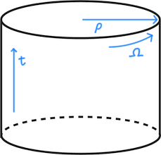
Figure 1: AdS space

The CFT primary field which is dual to the bulk scalar is ${\cal O}_{\Delta}(t,\Omega)$ with the conformal dimension $\Delta=d/2+\sqrt{m^{2}+d^{2}/4}$ on the cylinder $ds^{2}_{cyl}=-dt^{2}+d\rho^{2}+\sin^{2}(\rho)d\Omega_{d-1}^{2}$.

The BDHM relation [4],

$$\lim_{z\rightarrow 0}{\phi(t,z,\Omega)\over z^{\Delta}}\sim{\cal O}_{\Delta}(t,\Omega),\,\,\,\mbox{ where $z=\pi/2-\rho$}$$ (2.4)

is the relation between the bulk field and the CFT scalar primary field. Using this relation and the bulk equations of motion, the bulk local field is reconstructed from the CFT primary field, as in the HKLL bulk reconstruction [13], in the large $N$ limit where the bulk theory is free. Thus, in this limit, we can explicitly study the bulk local operators from the CFT viewpoint. For this study, it is more convenient to express the operators or the states in the energy eigen state basis. This was done explicitly in [26] and the relation between the bulk local operators and the CFT primary fields is clear as shown in the Appendix A.

2.2 Reconstruction of bulk local operators

Below, using the HKLL bulk reconstruction formula [13], we will see how the bulk local operator is reconstructed. The results are rather simple. For example, the bulk local state at center is given by time evolution of uniformly distributed CFT states which are localized at the fixed time. Thus, we conclude that through this kind of analysis, we understand how the bulk local operator emerges.

Let us consider the bulk local operator at the center of AdS space, i.e. $\phi(\rho=0)$, at $t=0$ and the corresponding bulk local state at the center, $\phi(\rho=0){\left|0\right\rangle}$. It was shown in [29] that this bulk state is essentially equivalent to the following CFT state: $\int_{S^{d-1}}d\Omega\,e^{i{\pi\over 2}H}{\cal O}_{\Delta}(\Omega)|0\rangle$, i.e.

$$\phi(\rho=0){\left|0\right\rangle}=\int_{S^{d-1}}d\Omega\,e^{i{\pi\over 2}H}{\cal O}_{\Delta}(\Omega)|0\rangle,$$ (2.5)

up to an overall numerical constant (Figure 2).

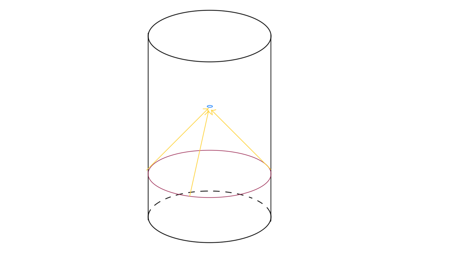
Figure 2: The blue dot represents the center ($\rho=0$) at $t=0$ where we consider the bulk local state $\phi(\rho=0){\left|0\right\rangle}$. The red circle represents the $t=-\pi/2$ slice on the boundary where we consider $\int_{S^{d-1}}d\Omega\,{\cal O}_{\Delta}(\Omega)|0\rangle$, which is equivalent to the bulk local state by the time evolution. The yellow lines represent the light-like trajectories from the $t=-\pi/2$ slice on the boundary to the center at $t=0$.

More precisely, this expression is valid only for $\Delta=d-1$ and the general expression, which includes the time-derivatives, is given in the Appendix A. This CFT state $\int_{S^{d-1}}d\Omega\,e^{i{\pi\over 2}H}{\cal O}_{\Delta}(\Omega)|0\rangle$ at $t=0$ is obtained from the CFT state $\int_{S^{d-1}}d\Omega\,{\cal O}_{\Delta}(\Omega)|0\rangle$ at $t=-\pi/2$ by the time evolution to $t=0$. (The operator $\int_{S^{d-1}}d\Omega\,{\cal O}_{\Delta}(\Omega)$ is a CFT local state averaged over the whole space and then it is invariant under the rotation.)

This equivalence, or the bulk reconstruction, has a simple picture if we regard the CFT local operators as the bulk operators on the boundary using the BDHM relation, The bulk local operator at the center is formed by the boundary operators located on $S^{d-1}$ at $t=-\pi/2$, which are reached to the bulk local operator by the (spherical symmetric) light-like rays.

We note that the bulk local operator contains arbitrary high momentum modes because it is supported on a point, thus the mass of the bulk scalar field is negligible, which is responsible for the light-like behavior.

One might think this is different from the well-known HKLL bulk reconstruction [13], in which the bulk local operator is constructed from the CFT operators on the time-interval $-\frac{\pi}{2}\leq t\leq\frac{\pi}{2}$, not just on $t=-\pi/2$. Below, we will show that the HKLL bulk reconstruction indeed give the same picture by a careful analysis. Of course, this is not surprising because the HKLL bulk reconstruction and the bulk reconstruction given in Appendix A are equivalent. The HKLL bulk reconstruction of the bulk local operator at the center is the following:

$$\phi(\rho=0,t=0)=\int_{-\frac{\pi}{2}}^{\frac{\pi}{2}}dt^{\prime}\int_{S^{d-1}}d\Omega^{\prime}\,K(\Omega^{\prime},t^{\prime}){\cal O}_{\Delta}(\Omega^{\prime},t^{\prime}),$$ (2.6)

where the smearing function $K(\Omega^{\prime},t^{\prime})$ for $d=\mbox{odd}$ is given by

$$K(\Omega,t)\sim{1\over(\cos t)^{d-\Delta}}$$ (2.7)

up to a constant depending on $\Delta$ and $d$. For $d=\mbox{even}$, the smearing function is $K(\Omega,t)\sim{\log t\over(\cos t)^{d-\Delta}}$. If $d-\Delta\geq 1$, an integration $\int dt^{\prime}K(\Omega^{\prime},t^{\prime})$ is divergent near $|t^{\prime}|=\pi/2$, which means that the contributions of the CFT local operator ${\cal O}_{\Delta}(\Omega^{\prime},t^{\prime})$ in the HKLL reconstruction (2.6) is negligible for $|t^{\prime}|<\pi/2$. Thus the time integration is localized on $t^{\prime}=\pm\pi/2$:

$$\phi(\rho=0,t=0)\sim\int_{S^{d-1}}d\Omega^{\prime}\,\left({\cal O}_{\Delta}(\Omega^{\prime},t=-\pi/2)+{\cal O}_{\Delta}(\Omega^{\prime},t=\pi/2)\right),$$ (2.8)

as shown in Figure 3. (Again, this expression is valid only for $\Delta=d-1$ and the general expression, which includes the time-derivatives, is given in the Appendix A.)

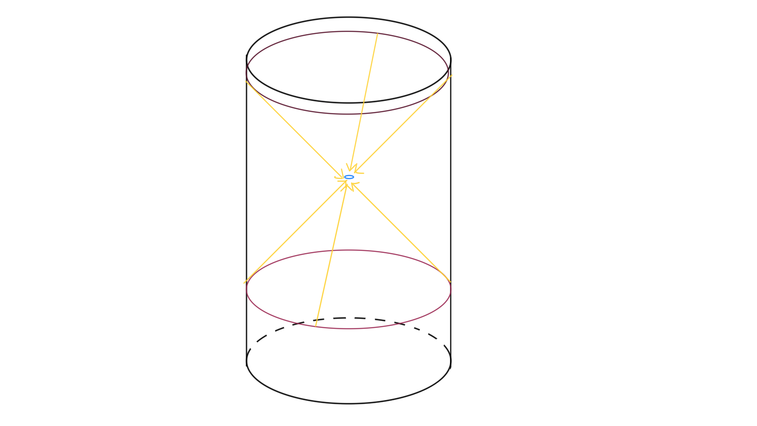
Figure 3: The bulk reconstruction by (2.8). Instead of the interval $-\pi/2\geq t\geq\pi/2$, only the contributions from the $t=\pm\pi/2$ slices are needed to reconstruct the bulk local operator.

The previous picture is obtained for the bulk local state $\phi(\rho=0,t=0){\left|0\right\rangle}$ if we notice that the CFT operator $\int_{S^{d-1}}d\Omega^{\prime}\,{\cal O}^{+}_{\Delta}(\Omega^{\prime},t)$, where ${\cal O}^{+}_{\Delta}(\Omega^{\prime},t)$ is the positive energy modes of ${\cal O}_{\Delta}(\Omega^{\prime},t)$, at $t=\pi/2$ is same as the one at $t=-\pi/2$ up to a overall constant because of the time periodicity in the large $N$ limit and the parity invariance.

Note that this localization of the integration is indeed required by the bulk causality and the BDHM relation ${\cal O}_{\Delta}(\Omega,t)\sim\phi(\rho=\pi/2,\Omega,t)$, i.e. the identification of the CFT primary operator as the bulk operator at the boundary. The bulk operator at the center $\phi(\rho=0,t=0)$ should be independent from the bulk operator at the spacetime point outside the light cone of the center $\{\rho=0,t=0\}$ however, the boundary point $\{\rho=\pi/2,\Omega,t\}$ is obviously not within the light cone for $|t|<\pi/2$. Thus, the bulk reconstruction of $\phi(\rho=0,t=0)$ should commute with any local operator constructed from ${\cal O}_{\Delta}(\Omega,t)$ for $|t|<\pi/2$. Thus, the CFT operators on ${\cal O}_{\Delta}(\Omega,t)$ for $|t|=\pi/2$ should be dominant for the reconstruction of the bulk local operator and our picture is natural and consistent with the bulk causality. In this sense, we can say that the HKLL reconstruction formula (2.6) is correct, but misleading.

For $d-\Delta<1$, the HKLL reconstruction seems to give a completely different picture because the smearing function is zero on $t=\pm\pi/2$. However, even for this case, the above picture, in which only the CFT operators on an arbitrary small region containing $t=\pm\pi/2$ are relevant, is correct as we will see in appendix A.3, essentially because $t=\pm\pi/2$ is the branch point, thus the singular point, of the hypergeometric function appeared in the HKLL reconstruction.

Next, we will consider the bulk local operator which is not at the center, $\phi(\rho,\Omega,t=0)$, and the CFT operator corresponding to it. For this, the HKLL reconstruction formula was obtained by the conformal map from the formula for the center [13]. Thus, the above picture is also true for this case. More explicitly, the reconstruction formula is same as (2.6),

$$\phi(\rho,\Omega,t=0)=\int dt^{\prime}\int d\Omega^{\prime}\,K(\rho,\Omega,\Omega^{\prime},t^{\prime}){\cal O}_{\Delta}(\Omega^{\prime},t^{\prime}),$$ (2.9)

where the integrations of $t^{\prime}$ and $\Omega^{\prime}$ were taken over the boundary points which are space-like separated from the bulk operator insertion point $\{\rho,\Omega,t=0\}$ and the smearing function is

$$K(\rho,\Omega,\Omega^{\prime},t^{\prime})\sim{1\over(d(\rho,\Omega,\Omega^{\prime},t^{\prime}))^{d-\Delta}},$$ (2.10)

where $d(\rho,\Omega,\Omega^{\prime},t^{\prime})$ is the geodesic distance between the point $\{\rho,\Omega,t=0\}$ and the boundary point $\{\rho=\pi/2,\Omega^{\prime},t^{\prime}\}$. The geodesic distances are zero for the the boundary points connected to the bulk operator insertion point by the light-like trajectories, then the integration is localized on such boundary points. This means that the bulk local operator is composed by the CFT primary operators on such boundary points and the bulk reconstruction picture above is true for this case also.

2.3 Bulk wave packet moving in a particular direction

We have seen that a bulk local state is represented by CFT primary states integrated on a space-like surface, which is regarded as a time-slice with an appropriate definition of a time. In this section we will consider CFT primary operators integrated on a small and an almost point like region, instead of the space-like surface. We will see that the bulk local state moving in a particular direction corresponds to a state obtained by acting such a CFT operator on the vacuum.

We will consider the following operator:

$$\phi_{A}\equiv\int_{S^{d-1}}d\Omega\,f_{A}(\Omega)\,e^{i{\pi\over 2}H}{\cal O}_{\Delta}(\Omega)e^{-i{\pi\over 2}H},$$ (2.11)

where $f_{A}(\Omega)$ is a function (effectively) supported on a small region $A$ in $S^{d-1}$. More explicitly, we take a small ball shaped region with radius $l_{A}$ for $A$ and the Gaussian distribution for $f_{A}(\Omega)$. If we averaged the position of $A$ over the whole space $S^{d-1}$, this operator becomes the bulk local operator at the center, as we have seen. Precisely speaking, we need to act some derivatives on ${\cal O}_{\Delta}(\Omega)$ in (2.11) as explained in Appendix A.1. Below, we will omit such derivatives for the notational simplicity.

Thus, it is natural to think $\phi_{A}$ represents a part of the bulk local operator at the center. Indeed, in [29], it was shown that the $\phi_{A}{\left|0\right\rangle}$ is a bulk (almost) local state or a wave packet at the center moving in the radial direction. Note that the bulk local operator should be smeared over a small, but larger than the Plank scale region.

Furthermore, the following operator:

$$\phi_{A}(z)\equiv\int_{S^{d-1}}d\Omega\,f_{A}(\Omega)\,e^{i{z}H}{\cal O}_{\Delta}(\Omega)e^{-i{z}H},$$ (2.12)

was shown to be a bulk wave packet moving inward in the radial direction at $\rho=\pi/2-z$, where $\pi/2\geq z>0$, and $\Omega$ is the location of the small region $A$, [29]. Of course, this CFT operator is the time evolution of the CFT operator $\int_{S^{d-1}}d\Omega\,f_{A}(\Omega)\,{\cal O}_{\Delta}(\Omega)$ at $t=-z$ to $t=0$. (Figure 4.)

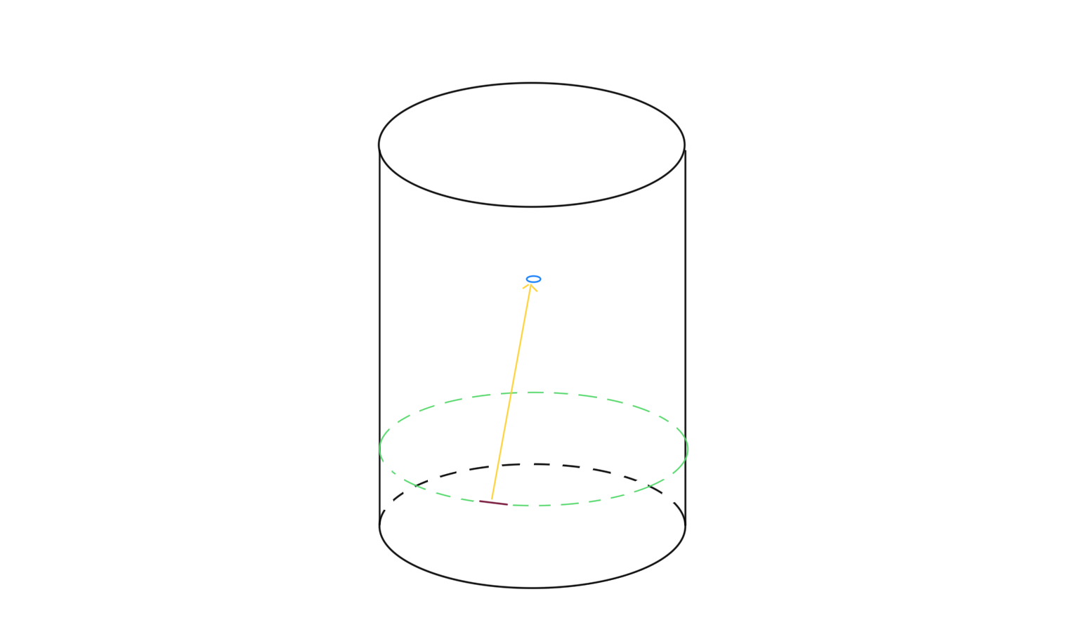
Figure 4: The bulk wave packet moving toward the center. The small region $A$, which is represented by small red curves, is on the $t=-\pi/2$ slice on the boundary, which is represented by the green dotted circle. The yellow line to the center is the light-like trajectory from $A$ and represents the wave packet.

This result also has a simple interpretation in the bulk picture as before. The CFT operator of $\phi_{A}$ is regarded as the bulk operator on the boundary smeared over the region $A$ by the Gaussian distribution, but not smeared for the radial direction. (More precisely, it should be smeared for the time-direction with some length scale which is very small, but larger than the Plank scale [29].) This is a kind of bulk wave packets. A usual wave packet is defined by choosing a particular momentum. For our case, the momentum for the angular direction is ${\cal O}(1/l_{A})$, but the momentum for the radial direction is not constrained, then most of them are much larger than $1/l_{A}$. Thus, the operator is a linear combination of wave packets and most of them are moving in the radial direction. This means that at $t=0$ the wave packet is at $\rho=-z$ and the $\phi_{A}(z)$ represents the small wave packet localized at the center moving in the radial direction.

On the other hand, in the CFT picture, the operator localized in the region $A$ at $t=-\pi/2$ is spread out spherically $(S^{d-2})$ in space ($S^{d-1}$) at $t=0$. Here, very large momentum modes up to $1/l_{A}$ are contained in the operator and this spreading is light-like [31]. Thus, the operator at $t=0$ is localized in a ”great circle” in $S^{d-1}$. For the $d=2$ case, the ”great circle” is two antipodal points in $S^{1}$. (Figure 5.)

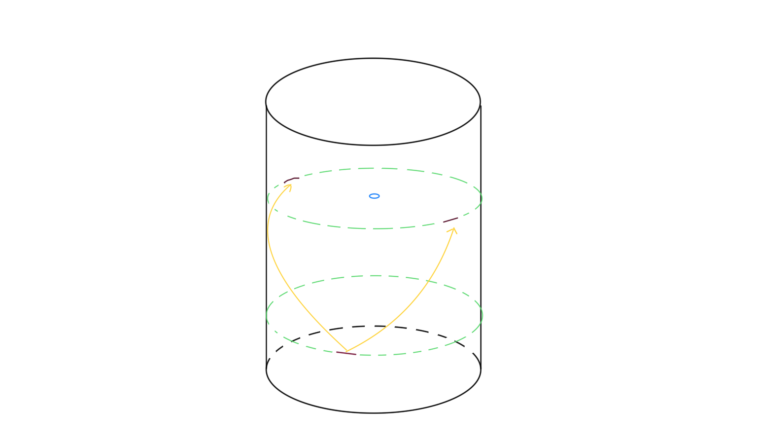
Figure 5: The CFT picture of Figure 4. Here, the two green dotted circles represent the $t=0$ and $t=-\pi/2$ slices. The two yellow curves on the boundary from $A$ to the antipodal points on the boundary are the light-like trajectories from $A$ and represent the wave packet in the CFT picture.

Even for $d>2$, if we take $A$ in the definition of $\phi_{A}$ as an ellipsoid which is squeezed in a particular direction, then the operator $\phi_{A}$ is localized on the two antipodal points in $S^{d-1}$ in the CFT picture. Furthermore, this $\phi_{A}$ is still localized at the center in the bulk picture if we take the length scales of the ellipsoid much larger than the cut-off scale (smearing) of the local operator as like the ball shaped region case.

This implies that this bulk localized wave packet is constructed as the entangled state in CFT, which can be written schematically as $({\left|1\right\rangle}\otimes{\left|0\right\rangle}+{\left|0\right\rangle}\otimes{\left|1\right\rangle})\otimes{\left|\rm others\right\rangle}$, where ${\left|1\right\rangle}$ is the one particle state, ${\left|0\right\rangle}$ is no excitation state and, the first and the second kets represent the states localized on the two antipodal points. On the other hand, a linear combination of CFT primary states (with a small number of derivatives) at two different points is a linear combination of bulk states localized on two points on the boundary, not inside, even in the bulk picture, although this is also an entangled state.

We have seen that the bulk local operator moving in the radial direction is represented by $\phi_{A}(z)$ in the CFT picture. It is easy to generalize this to the bulk local operator moving in an arbitrary direction by considering a conformal map, which maps the bulk local operator at the center to an arbitrary point, say $\rho=\rho_{1},\Omega=\Omega_{1},t=t_{1}$ [13]. This conformal map changes the $t=-\pi/2$ slice $(S^{d-1})$ on the boundary to the slice on $t=-\pi/2+\delta t(\Omega)$ where $\delta t(\Omega)$ represents the tilt in time direction. Thus, if we generalize $\phi_{A}(z)$ to

$$\phi_{A}(z) \equiv\int_{S^{d-1}}d\Omega\,f_{A}(\Omega)\,e^{i{z}H}{\cal O}_{\Delta}(\Omega,t=\delta t(\Omega))e^{-i{z}H}$$ (2.13)

$$=\int_{S^{d-1}}d\Omega\,f_{A}(\Omega)\,e^{i{(z+\delta t(\Omega))}H}{\cal O}_{\Delta}(\Omega)e^{-i{(z+\delta t(\Omega))}H},$$ (2.14)

this $\phi_{A}(z)$ represents the bulk local operator which moving from the small region $A$ on $t=-\pi/2$ slice to the point $\rho=\rho_{1},\Omega=\Omega_{1},t=t_{1}$ light-likely where $z$ parametrizes the light-like trajectory. The wave packet is at the the small region $A$ for $z=0$ and at the bulk point $\rho=\rho_{1},\Omega=\Omega_{1},t=t_{1}$ for $z=\pi/2+t_{1}$. This picture is also checked in the operator formalism as we will see in the Appendix A.2.

In summary, we have the following simple and intuitive picture of the reconstruction of the bulk local operator or state in AdS/CFT around the vacuum. The bulk local state at a spacetime point $P$ is represented by the CFT primary state integrated over $C$, where the region $C$ is the intersection of the light rays emanating from $P$ to the past and the boundary of AdS spacetime. The wave packetof the bulk local state at the point $P$ is represented by the CFT primary state integrated over $A$, where very small region $A$ is the intersection of trajectory of the wave packet to the past and the boundary of AdS spacetime. For the bulk local operator instead of the state, we just need to take into account the light rays to the future adding to ones to the past .

2.3.1 Causalities and duality

Here, we will check that the above picture is consistent with the causalities and the duality. For the light-like trajectory from a boundary point toward the center, as drawn in Figure 4 and Figure 5, it was already shown in [29] that the bulk causality is consistent with the CFT picture. Indeed, both in the CFT and bulk pictures, the (light-like) wave packets reach the boundary at the antipodal point at the same time. This result was already shown in [32] where, in AdS spacetime, any light-like trajectory from a boundary point at $t=0$ reaches the antipodal point on the boundary at $t=\pi$. Such light-like trajectory can be always on the boundary, which is realized in the CFT picture. Thus, any light-like trajectory from a boundary point in the bulk picture and the corresponding two light-like trajectories in our CFT picture reach the antipodal boundary point at same time, then this picture is consistent with the causality. Furthermore this is the only possibility for the consistent CFT dual to the bulk wave packet if we require the causalities both in the bulk and the CFT pictures. This is because the bulk wave packet on the boundary, which is realized when $t=0$ or $t=\pi$, is regarded as a wave packet composed by the CFT primary field and the speed of the propagation is bounded by the speed of light in the both pictures. This implies that in the CFT picture also, the corresponding wave packets should be on the light-like trajectories.

2.3.2 Locality in radial direction

Here, we will discuss how the locality in radial direction appears in our picture of the bulk reconstruction. Note that the discussions here are only for the free theory limit in the bulk. For the spherical symmetric states (e.g. in Figure 2), the bulk local state integrated over the sphere $S^{d-1}$ at the radial coordinate $\rho=\pi/2-z_{0}$ corresponds to the CFT primary state on the time $t=-z_{0}$ slice integrated over the sphere $S^{d-1}$. This implies that the radial locality is same as the locality in the time direction in this setup. In order to realize this, it is needed that the primary fields with different times are (almost) independent (for $-\pi/2<t<\pi/2$). This is only possible for the theory with (almost) infinite degrees of freedoms like the large $N$ gauge theory. Indeed, for the free CFT or a theory with a finite degrees of freedom, the fields with different time are related by the equation of motions and they are not independent.

For the non-spherical symmetric case, the radial location of the bulk local operator is related to the time coordinate of the CFT primary fields although the relation is not direct. The independence between CFT primary fields at different times are important for this case also. This independence means that commutator of the CFT primary fields at different times vanish. For the free CFT, the commutators of two free fields does not vanish if the one field is in the light-cone of the other field. Of course, this property is same for any CFT, however, for the non-trivial CFT, a commutator of the CFT primary fields is non-zero value on the light-cone and is diverging at $\sin t=0$ where $t$ is the time difference between the two fields, as was explicitly shown for $\Delta=d/2$ [31]. This divergence is regularized by the smearing of the local operator with a cut-off and the normalized commutator by this cut-off is effectively zero for CFT primary fields at different times.

Note that this discussion can be applied for any non-trivial CFT. The holographic CFT is special because it behaves like the generalized free field, which implies that the product of the CFT primary fields are independent each other. In the commutator or the OPE languages, this is reflected in the fact that the contribution proportional to the identity operator is dominant in the large $N$ limit. Thus, in our picture, the bulk locality in radial direction is essentially mapped to the locality in the time direction in the CFT.

2.4 Bulk operators correspond to CFT operators in a region

We have seen how bulk local operators are mapped to the CFT operators. We can also map the CFT operators supported in a region $A$ in $S^{d-1}$ on $t=0$ slice, $\{{\cal O}_{A}\}$, to the bulk operators on $t=0$ slice [29]. In particular, we will consider what is the (smallest) bulk region $a$ corresponding to the CFT region $A$, where the bulk operators corresponding to $\{{\cal O}_{A}\}$ are supported in the bulk region $a$. (Note that if the subregion duality [35][39] is correct, these bulk operators should be equivalent to $\{{\cal O}_{A}\}$, i.e. any bulk operator supported in the region $a$ should correspond to some ${\cal O}_{A}$, in the low energy approximation. Here we do not assume this version of the duality. We will call it the strong version of the subregion duality, in order to distinguish it to a version of the subregion duality where the correspondence between the density matrices is required, as we will explain later.)

We note that any CFT operator (at $t=0$) can be generated by the CFT primary operator integrated over the spacetime with a weight $f(\Omega,t)$:

$$\phi_{f}\equiv\int dt\int_{S^{d-1}}d\Omega\,f(\Omega,t){\cal O}_{\Delta}(\Omega,t),$$ (2.15)

because derivatives of the primary field can be represented by taking the distribution $f(\Omega,t)$ as derivatives of the (smeared) delta function.

Let us investigate which $\phi_{f}$ is a CFT operator supported in the region $A$. It is obvious that $\phi_{f}$ is supported in the region $A$ if $f(\Omega,t)$ is nonzero only in the causal diamond of the region $A$ in the CFT picture because of the causality (Figure 6).

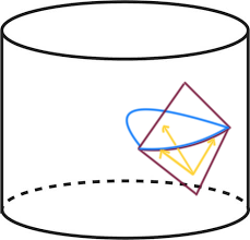
Figure 6: The red lines represent the region $A$ on $t=0$ slice and its causal diamond on the boundary. The causal wedge of $A$ on $t=0$ slice is the bulk region inside of the blue curve. The yellow lines are light-like trajectories. The one of the these lines toward the inside the bulk represents the wave packet in the causal wedge. The other two are on the boundary and represent the wave packets in the CFT picture.

More generally, as we have seen in the previous section, a small wave packet of CFT local operators at $(\Omega_{0},t_{0})$ can behave like two light-rays emitted from there to opposite directions in space $S^{d-1}$. If both of the two light rays reach the region $A$ on $t=0$ slice, this wave packet of CFT local operators is supported in the region $A$. Thus, by taking $f(\Omega,t)$ as this wave packet at $(\Omega_{0},t_{0})$, $\phi_{f}$ is an operator supported in the region $A$. It is difficult to expect other possibilities of choice of $f(\Omega,t)$ to obtain $\phi_{f}$ is an operator supported in the region $A$ because the propagation is generic other than the causality constraints. Thus, below we assume that $\phi_{f}$ is a CFT operator supported on the region $A$ only if $f(\Omega,t)$ is a linear combination of such wave packets.

2.4.1 Ball shaped region

First, we take the subregion $A$ as a ball shaped region in $S^{d-1}$. For this case, in the CFT picture, the above wave packets are in the causal diamond if the two light rays reach the region $A$ on $t=0$. Thus, $\phi_{f}$ is supported on the region $A$ only if $f(\Omega,t)$ is nonzero only in the causal diamond of the region $A$ (Figure 6).

In the bulk picture, as we have seen in the previous section, the bulk operator corresponding to such $\phi_{f}$ represents a linear combination of wave packets moving in arbitrary directions in bulk space. Such wave packets in the bulk can reach only the causal wedge of $A$ on $t=0$. This means that any CFT operator supported on the region $A$ corresponds to a bulk operator supported on the causal wedge of $A$. Note that the causal wedge (on $t=0$) is the bulk region inside the Ryu-Takayanagi surface of $A$ [34], i.e. the entanglement wedge.

2.4.2 Subregion duality, error correction code and AdS-Rindler reconstruction

It is important that there exist bulk operators supported in the causal wedge of $A$ which can not be reconstructed from CFT operators supported in the region $A$. Indeed, there are bulk light-rays or null-geodesics starting from a boundary point to another boundary point through the causal wedge of $A$ such that both of the two boundary points are not the (CFT) causal diamond of $A$. Then, the wave packets along these can not reconstructed from CFT operators supported in the region $A$. Note that in the large $N$ (free bulk theory) limit we considered in the paper, any state with a (Plank scale) cut-off of the energy, which is realized by a smearing of the local operator, can be regarded as a low energy state, and states of the bulk free theory and the CFT (which is approximated as the generalized free theory) are identical. In other words, we restricted only the low energy states in this paper. Thus, there is no alternative reconstruction from CFT operators supported in the region $A$.

This has implications for the subregion duality [35]-[39]. Indeed, this violates a strong version of the subregion duality, which claims that any bulk operator supported in the causal wedge of $A$ can be reconstructed from the low energy CFT operators supported in the region $A$, for this set-up. (We consider only the low energy CFT operators in this paper.) Problems of the strong version of subregion duality related to such null-geodesics were already raised in [30]. In [30], it was stated that some non-local operators could solve the problems although there are no concrete arguments for this. In our setup there are no such operators solving the problem because the low energy CFT spectrum is given and the operators associated to the null-geodesics are explicitly given by the CFT primary operators, which are not supported in the region $A$. Thus, the strong version of the subregion duality is not valid. Note that this duality is assumed in many papers, for example, in [41] for the entanglement wedge reconstruction.

The strongest reason to believe this strong version of the subregion duality may be the HKLL AdS-Rindler reconstruction [13], by which the correlation function of the bulk local operators in the AdS-Rindler patch is reproduced from certain CFT operators in the corresponding subregion $A$ [42]. This seems to implies that the bulk local operators can be reconstructed from CFT operators in a subregion, not in the whole space $S^{d-1}$ as we have seen. However, the HKLL AdS-Rindler reconstruction assume that the BDHM relation holds even in the AdS-Rindler patch. This assumption was recently shown to be violated because of the finite $N$ effect [44], and the HKLL AdS-Rindler reconstruction is not correct. Thus, $\phi(x)\neq\phi_{\rm Rindler}(x)$, where we denote by $\phi_{\rm Rindler}(x)$ the part of the bulk local operator $\phi(x)$ which can be reconstructed from the CFT operators supported on the Rindler subregion $A$ in the boundary. Note that the part of $\phi(x)$ which can not be reconstructed from CFT on $A$ is related to the horizon to horizon null-geodesics in [44].

Note that the quantum error correction code proposal [43] is partly based on the claim that $\phi(x)=\phi_{\rm Rindler}(x)$ in the low energy theory, thus this proposal is not realized in holographic CFTs. Even from the following discussion using the HKLL bulk reconstruction (2.6), it is easy to see that $\phi(x)=\phi_{\rm Rindler}(x)$ is not valid. By inserting (A.11) into (2.6) and integrating over the $S^{d-1}$ first, we can see that the bulk local operator at the center $\phi(\rho=0)$ only contains the modes with $l=0$, i.e. the spherical symmetric modes $a_{n00}$. These modes are generically low energy modes. On the other hand, it is obviously impossible to construct the operator, which only contains the spherical symmetric modes, from the CFT operators supported on a subregion in $S^{d-1}$. This means that $\phi_{\rm Rindler}(\rho=0)$ of the AdS-Rindler reconstruction is different from $\phi(\rho=0)$.

Of course, these discussions of the AdS-Rindler reconstruction are related to our picture in this paper. In particular, as we have seen, the wave packet reconstructed from a small subregion in CFT is a part of a bulk local operator reconstructed from a whole space $S^{d-1}$, i.e. the bulk local operator is obtained by assembling such wave packets for small subregions in whole space. The null-geodesics correspond to such wave packets. The AdS-Rindler reconstruction uses only the wave packets corresponding to the half of $S^{d-1}$.

The AdS-Rindler reconstruction and our bulk reconstruction picture lead another version of the subregion duality, in which the (low energy) CFT operators supported in region $A$ is dual to the part of bulk operators in the bulk theory in the AdS-Rindler patch $M_{A}$. We stress again that these are not equivalent to the bulk operators supported on AdS-Rindler patch $M_{A}$ in the bulk theory in the global AdS. By tracing out the states supported in $\bar{A}$, this duality becomes the correspondence between the density matrix $\rho_{A}$ of the region $A$ in CFT and the density matrix $\rho_{M_{A}}$ of the AdS-Rindler patch in the “bulk theory” which includes the part of the bulk local operators.

2.5 Disjoint regions

Now, we will take the subregion $A$ as a space which is (topologically) different from the ball-shaped space. For the concreteness of the discussion, we will take $A$ as a sum of disjoint two intervals $A_{1},A_{2}$ for $d=2$ CFT. (A ball shaped region is an interval for $d=2$.) For this case, we can apply the previous discussion on the ball shaped region to each $A_{i}$. Then, we find that there are CFT operators supported in the region $A=A_{1}\cup A_{2}$ correspond to bulk operators supported in the causal wedge of $A_{1}$ or $A_{2}$. Other than these, there are other kinds of CFT operators supported in the region $A$. Indeed, the time evolution of the CFT local operator at $(\Omega_{0},t_{0})$ to $t=0$ is supported in the region $A$ if the intersection of the light cone of $(\Omega_{0},t_{0})$ and the $t=0$ slice in CFT is contained in $A=A_{1}\cup A_{2}$. The bulk operators corresponding to such CFT operators are the wave packets emitting from $(\Omega_{0},t_{0})$ to the bulk in arbitrary directions. Then, these bulk operators are supported in the bulk region between the two minimal surfaces connecting $A_{1}$ and $A_{2}$ (Figure 7)

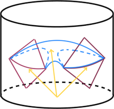
Figure 7: Two intervals (region $A$) and their causal diamonds on the boundary are represented by red lines. Inside the blue curve are the entanglement wedge and inside the dotted blue curves are causal wedges. The two light rays, represented by the yellow lines on the boundary, reach the region $A$ at $t=0$. Thus, the operator is supported on the region $A$. The other yellow line, which represents the bulk picture of them, can reach the entanglement wedge outside the causal wedges at $t=0$.

as shown in [29].

This region coincides with the entanglement wedge [35]-[37] if the sizes of $A_{i}$ are sufficiently large compared with the distance between $A_{1}$ and $A_{2}$. It had been difficult to understand how to reconstruct the bulk operators outside the causal wedge. It is interesting that we can explicitly reconstruct it here.

If the sizes of $A_{i}$ are sufficiently small, it is believed that the entanglement wedge becomes the causal wedge and these bulk operators reconstructed from the CFT operators supported in $A$ are outside the entanglement wedge of $A$. This phase transition like behavior does not appear in our case and there seem some contradictions. However, the Ryu-Takayanagi surface appears in the computation of the entanglement entropy of region $A$ using the replica trick in the path-integral, and there are no concrete arguments that this implies that the relation between the Ryu-Takayanagi surface and the bulk region in which the bulk operators corresponding to $A$ are supported. Furthermore, it is difficult to determine in which states the bulk modular Hamiltonian, which appears in the relative entropy [38], acts. Thus, there will be no contradictions between our results and the phase transition.

3 Generalization to asymptotic AdS

In this section, we will generalize our picture of the reconstruction of the bulk local state or operators to the asymptotic AdS spacetime. Here, we consider, instead of the vacuum, a CFT state ${\left|g_{\mu\nu}\right\rangle}$ which corresponds to the semi-classical asymptotic AdS spacetime background of the bulk theory. First, we will consider a part of the geometry in which the causal structure is trivial and there is no horizon for simplicity. We expect that the BDHM relation (2.4) is hold for this case also and we assume it. We also assume as usual that in the large $N$ limit the fluctuations around this background in the bulk theory is free theory on this asymptotic AdS spacetime. We only consider this perturbative approximation.

Let us consider a bulk local state at a point $p$ on a time slice ($t=0$) and the backward-time evolution of it. (Here, the time slice is defined by the dilatation operator, for example.) As in the AdS background, this evolutions is on the past light-cone of the point $p$ because the local operator contains arbitrary high-momentum modes. Then, the bulk local state is represented as the bulk local operators acting on ${\left|g_{\mu\nu}\right\rangle}$ integrated over a submanifold $M_{p}^{-}$ on the boundary of the asymptotic AdS spacetime, where $M_{p}^{-}$ is the intersection of this past light-cone and the boundary of the asymptotic AdS spacetime. Using the BDHM relation, we can replace the bulk local operators on the boundary as the CFT primary operators. Thus, the bulk local state at $p$ is reconstructed from the CFT primary operators acting on ${\left|g_{\mu\nu}\right\rangle}$ integrated over $M_{p}$ which we regard a subregion in the spacetime for CFT.

Instead of the bulk local state $\phi(x){\left|g_{\mu\nu}\right\rangle}$, we can consider bulk local operator $\phi(x)=\phi(x)^{+}+\phi(x)^{-}$ itself. Note that $\phi(x){\left|g_{\mu\nu}\right\rangle}=\phi(x)^{+}{\left|g_{\mu\nu}\right\rangle}$ determines $\phi(x)^{+}$ up to an overall phase in the large $N$ limit. In order to construct $\phi(x)=\phi(x)^{+}+\phi(x)^{-}$, we need to give this phase. Note that the time-evolution is symmetric for past and future. Thus, as for the AdS spacetime, we expect that the bulk local operator is reconstructed from the CFT primary operators integrated over $M_{p}=M_{p}^{+}\cup M_{p}^{-}$ where $M_{p}^{+}$ and $M_{p}^{-}$ is for the future and past light cones, respectively.

The bulk operator corresponding to the wave packet moving along a light-like trajectory is also realized by a CFT operator, as for the AdS spacetime. Indeed, the positive energy parts of the CFT operator $\phi_{A}(z)$ defined by (2.14), which was constructed for AdS spacetime, represents the wave packet moving into the bulk in the direction determined by the tilt $\delta t(\Omega)$ near $z=0$, i.e. on the boundary because the near the boundary the BDHM relation is assumed to be hold. Then, this represents the wave packet moving along the light-like trajectory of the asymptotic AdS geometry.

The causality and duality should be hold for the above wave packet also. Assuming the null-energy condition for the bulk theory, by the Gao-Wald theorem [32], any “fastest null geodesic” connecting two points on the boundary must lie entirely within the boundary. On the other hand, the wave packets should reach the boundary point at the same time in the both bulk and CFT pictures because of the duality and the BDHM relation. Thus, the bulk wave packet, which is on a light-like trajectory, should correspond to time-like trajectories on the boundary in the CFT picture. This is explained by the group velocity of the wave packet in the CFT picture is always lower than the speed of light in the vacuum. In the CFT picture, the asymptotic AdS spacetime is represented as the non-trivial CFT state ${\left|g_{\mu\nu}\right\rangle}$ and the speed of the wave packet will become lower in this medium. Of course, in the bulk picture this effects of medium is included in the metric and the velocity of the wave packet in the bulk is the speed of light. Thus, our picture of the bulk local operators for the asymptotic AdS spacetime is consistent with the Gao-Wald theorem [32].

3.1 Black hole

Let us consider the bulk reconstruction in the black hole in the asymptotic AdS spacetime. First, if we consider a (spherical symmetric) heavy star, then a bulk local state or a wave packet at the center of the star at $t=0$ will be reconstructed by CFT primary operators integrated on a region in $t<-\pi/2$ because of the time delay. If the star is nearer the black hole, the time delay is larger and can be arbitrary large, which means the whole past region $(t\leq 0)$ of the CFT space $S^{d-1}$ are needed to reconstruct the bulk local operators at $t=0$. This means that arbitrary large number of (approximately) independent fields are required because the bulk local operators at different points should be independent each other and different. Of course, this is impossible because $N$ is large, but finite although $N$ is formally infinite in the large $N$ expansion.

For the black hole, the bulk local states or a wave packets near the horizon, need infinitely many independent fields. This implies that the CFT can not reconstruct the bulk fields even outside the horizon. This is the same conclusion by the brick wall [52] [53] where some hypothetical boundary conditions were imposed. Here, even though we have not not imposed such boundary conditions, we conclude the shortage of the CFT states to reconstruct the bulk fields near the horizon, which strongly indicates the existence of the brick wall [52]/fuzzball [54] [55]/firewall [56] for the (single sided) black hole. Note that it is important to include the finite $N$ effects, which are the (strong) non-perturbative effects of the gravitational coupling from the bulk viewpoint, for this conclusion. Thus, this should be missed by the semi-classical analysis in the bulk.

Appendix A Map between bulk and CFT operators

In this Appendix, we will review the explicit map between the bulk and CFT operators in the energy eigen value basis [29] and show how the bulk wave packet is represented by the CFT primary operators. We also will see that only the CFT operators on $t=\pm\pi/2$ are relevant in the global HKLL reconstruction.

We expand the quantized bulk field $\phi$ with the spherical harmonics $Y_{lm}(\Omega)$,

$$\phi(t,\rho,\Omega)=\sum_{n,l,m}\left(\hat{a}_{nlm}^{\dagger}e^{i\omega_{nl}t}Y_{lm}(\Omega)+\hat{a}_{nlm}e^{-i\omega_{nl}t}Y^{*}_{lm}(\Omega)\right)\psi_{nl}(\rho),$$ (A.1)

where $\Omega$ represents the coordinates of $S^{d-1}$ and the energy eigen value $\omega_{nl}$ is given by

$$\omega_{nl}=2n+l+\Delta.$$ (A.2)

The “wave function” for the radial direction is given by

$$\psi_{nl}(\rho)=\frac{1}{{\cal N}_{nl}}\sin^{l}(\rho)\cos^{\Delta}(\rho)\,P_{n}^{l+d/2-1,\Delta-d/2}\left(\cos(2\rho)\right),$$ (A.3)

where $P_{n}^{\alpha,\beta}(x)$ is the Jacobi polynomial defined by

$$P_{n}^{\alpha,\beta}\left(x\right)={(-1)^{n}\over 2^{n}n!}(1-x)^{-\alpha}(1+x)^{-\beta}{d^{n}\over dx^{n}}\left((1-x)^{\alpha}(1+x)^{\beta}(1-x^{2})^{n}\right),$$ (A.4)

and the normalization constant ${\cal N}_{nl}$ is given by

$${\cal N}_{nl}=(-1)^{n}\sqrt{\frac{\Gamma(n+l+\frac{d}{2})\Gamma(n+1+\Delta-\frac{d}{2})}{\Gamma(n+l+\Delta)\Gamma(n+1)}}.$$ (A.5)

Note that $(-1)^{n}{\cal N}_{nl}\rightarrow 1$. for $n\rightarrow\infty$ with a fixed $l$. We will decompose the local operator in the bulk description to positive and negative energy modes as

$$\phi(t,\rho,\Omega)=\phi^{+}(t,\rho,\Omega)+\phi^{-}(t,\rho,\Omega),$$ (A.6)

where $\phi^{-}(t,\rho,\Omega)=(\phi^{+}(t,\rho,\Omega))^{\dagger}$.

Let us consider the scalar primary field ${\cal O}_{\Delta}(x)$, corresponding to $\phi(t,\rho,\Omega)$, in $CFT_{d}$ on $\mathbf{R}\times S^{d-1}$ where $\mathbf{R}$ is the time direction and the radius of $S^{d-1}$ is taken to be one. For a review of the $CFT_{d}$, see for example, [57, 58, 59]. We define the operator

$$\hat{{\cal O}}_{\Delta}=\lim_{x\rightarrow 0}{\cal O}^{+}_{\Delta}(x),$$ (A.7)

where ${\cal O}^{+}_{\Delta}(x)$ is the regular parts of ${\cal O}_{\Delta}(x)$ in $x^{\mu}\rightarrow 0$ limit which can be expanded by the polynomial of $x^{\mu}$.

The identification of the CFT states to the states of the Fock space of the scalar fields in AdS is explicitly given by the identification of the creation operators as

$$\hat{a}_{nlm}^{\dagger}=c_{nl}\,s^{\mu_{1}\mu_{2}\ldots\mu_{l}}_{(l,m)}P_{\mu_{1}}P_{\mu_{2}}\cdots P_{\mu_{l}}(P^{2})^{n}\hat{{\cal O}}_{\Delta}$$ (A.8)

where $c_{nl}$ is the normalization constant, which was given in [26], the translation operation $P^{\mu}$ act on an operator such that $P^{\mu}\phi=[\hat{P}^{\mu},\phi]$ and $s^{\mu_{1}\mu_{2}\ldots\mu_{l}}_{(l,m)}$ is the normalized rank $l$ symmetric traceless constant tensor such that $Y_{lm}(\Omega)=s^{\mu_{1}\mu_{2}\ldots\mu_{l}}_{(l,m)}x_{\mu_{1}}x_{\mu_{2}}\cdots x_{\mu_{l}}/|x|^{l}$.

Then, the bulk local operator is expressed as

$${\phi}^{+}(t=0,\rho,\Omega) =\sum_{n,l,m}\psi_{nl}(\rho)Y_{lm}(\Omega)\hat{a}_{nlm}^{\dagger}$$

$$=\sum_{n,l,m}\psi_{nl}(\rho)Y_{lm}(\Omega)c_{nl}s^{\mu_{1}\mu_{2}\ldots\mu_{l}}_{(l,m)}P_{\mu_{1}}P_{\mu_{2}}\cdots P_{\mu_{l}}(P^{2})^{n}\hat{{\cal O}}_{\Delta},$$ (A.9)

where only the CFT operators appear in the last line. It is convenient to write both of the bulk and CFT operators in the creation and annihilation operators, which are energy eigen operators. Indeed, from the BDHM relation [4] in our normalization:

$$\lim_{\rho\rightarrow\pi/2}{\phi(\rho,\Omega)\over\cos^{\Delta}(\rho)} =\sqrt{\pi\over 2}\sqrt{\Gamma(\Delta)\over\Gamma(\Delta+1-d/2)\Gamma(d/2)}{\cal O}_{\Delta}(\Omega),$$ (A.10)

we find

$${\cal O}_{\Delta}(\Omega,t)=\sum_{n,l,m}\psi_{nl}^{CFT}Y_{lm}(\Omega)e^{i\omega_{nl}t}\hat{a}_{nlm}^{\dagger}+h.c.=\sum_{n,l,m}\psi_{nl}^{CFT}\left(Y_{lm}(\Omega)e^{i\omega_{nl}t}\hat{a}_{nlm}^{\dagger}+Y^{*}_{lm}(\Omega)e^{-i\omega_{nl}t}\hat{a}_{nlm}\right),$$ (A.11)

where

$$\psi_{nl}^{CFT}\equiv\sqrt{{2\over\pi}{\Gamma(d/2)\over\Gamma(\Delta)\Gamma(\Delta+1-d/2)}}\sqrt{\Gamma(n+\Delta+1-d/2)\Gamma(n+l+\Delta)\over\Gamma(n+1)\Gamma(n+l+d/2)},$$ (A.12)

which reduces to a constant $\psi_{nl}^{CFT}=\sqrt{{2\over\pi}}$ for $\Delta=d/2$. For $n\rightarrow\infty$ with a fixed $l$, we have $\psi_{nl}^{CFT}\rightarrow\sqrt{{2\over\pi}{\Gamma(d/2)\over\Gamma(\Delta)\Gamma(\Delta+1-d/2)}}{n^{\Delta-d/2}}$.

Below we will see the relation between the bulk local operator at the origin and the CFT primary operator integrated over $S^{d-1}$. These two operators are given by

$${\phi}(t=0,\rho=0) =\sum_{n,l,m}\left(\hat{a}_{nlm}^{\dagger}Y_{lm}(\Omega)+\hat{a}_{nlm}Y^{*}_{lm}(\Omega)\right)\psi_{nl}(0)$$ (A.13)

$$=\sum_{n}(-1)^{n}\sqrt{\frac{\Gamma(n+\Delta)\Gamma(n+d/2)}{\Gamma(n+1)\Gamma(n+1+\Delta-d/2)}}\left(\hat{a}_{n00}^{\dagger}+\hat{a}_{n00}\right),$$ (A.14)

and

$$\int d\Omega\,{\cal O}_{\Delta}(\Omega,t) ={2\pi^{\frac{d}{2}}\over\Gamma(d/2)}\sum_{n}\psi_{n0}^{CFT}\left(e^{i(2n+\Delta)t}\hat{a}_{n00}^{\dagger}+e^{-i(2n+\Delta)t}\hat{a}_{n00}\right),$$ (A.15)

where we have used $Y_{00}(\Omega)=1$ and $\int d\Omega=2\pi^{d/2}/\Gamma(d/2)$. In particular, for $t=\pm\pi/2$, the latter becomes

$$\int d\Omega\,{\cal O}_{\Delta}(\Omega,t=\pm\pi/2)= \sum_{n}\sqrt{8\pi^{d-2}\over\Gamma(d/2)\Gamma(\Delta)\Gamma(\Delta+1-d/2)}\sqrt{\Gamma(n+\Delta)\Gamma(n+\Delta+1-d/2)\over\Gamma(n+1)\Gamma(n+d/2)}$$

$$\times(-1)^{n}\left(e^{\pm i\frac{\pi}{2}\Delta}\hat{a}_{n00}^{\dagger}+e^{\mp i\frac{\pi}{2}\Delta}\hat{a}_{n00}\right),$$ (A.16)

Comparing these two expressions, we find

$$\phi^{+}(t=0,\rho=0)=C_{\Delta}e^{\mp i\frac{\pi}{2}\Delta}\int d\Omega\left(F_{\Delta}(\partial_{t})\,{\cal O}^{+}_{\Delta}(\Omega,t)\right)|_{t=\pm\frac{\pi}{2}},$$ (A.17)

where

$$C_{\Delta}=\sqrt{\Gamma(d/2)\Gamma(\Delta)\Gamma(\Delta+1-d/2)\over 8\pi^{d-2}},$$ (A.18)

$$F_{\Delta}(x)={\Gamma((-ix-\Delta+d)/2)\over\Gamma((-ix+\Delta-d+2)/2)}.$$ (A.19)

We have used $F_{\Delta}(\partial_{t})e^{i(2n+\Delta)t}={\Gamma(n+d/2)\over\Gamma(n+\Delta-d/2+1)}e^{i(2n+\Delta)t}$. On other hand, we find $F_{\Delta}(\partial_{t})e^{-i(2n+\Delta)t}={\Gamma(-n-\Delta+d/2)\over\Gamma(-n-d/2+1)}e^{-i(2n+\Delta)t}$ for the annihilation modes.

From (A.17), we obtain the following relation between the the bulk local state and the CFT state:

$$\phi(t=0,\rho=0){\left|0\right\rangle}=C_{\Delta}e^{\mp i\frac{\pi}{2}\Delta}\int d\Omega\left(F_{\Delta}(\partial_{t})\,{\cal O}_{\Delta}(\Omega,t)\right)|_{t=\pm\frac{\pi}{2}}{\left|0\right\rangle}.$$ (A.20)

This relation can be simplified for $\Delta=d-1$, which implies $F_{\Delta}(x)=1$, as

$$\phi(t=0,\rho=0){\left|0\right\rangle}=\sqrt{\Gamma(d/2)^{2}\Gamma(d-1)\over 8\pi^{d-2}}e^{\mp i\frac{\pi}{2}(d-1)}\int d\Omega\,{\cal O}_{\Delta}(\Omega,t=\pm\pi/2){\left|0\right\rangle}.$$ (A.21)

This expression, which implies (2.5) and the picture given in Figure 2, was obtained in [29]. Similarly, for $\Delta=d-1-m$ where $m$ is a positive integer, the relation can be also explicitly expressed as the integration localized on $t=\pm\pi/2$ because $F_{\Delta}(x)$ is a polynomial:

$$F_{\Delta=d-1-m}(x)=\prod_{m^{\prime}=0}^{m-1}((-ix-1+m-2m^{\prime})/2).$$ (A.22)

In [62], the corresponding results for the bulk local operators were obtained using the HKLL bulk reconstruction formula. For $\Delta=d-1+m$ where $m$ is a positive integer, we find the following simple relation:

$$F^{-1}_{\Delta}(\partial_{t})\phi(t=0,\rho=0){\left|0\right\rangle}=C_{\Delta}e^{\mp i\frac{\pi}{2}\Delta}\int d\Omega\,{\cal O}_{\Delta}(\Omega,t=\pm\pi/2){\left|0\right\rangle},$$ (A.23)

where $F^{-1}_{\Delta}(x)=\prod_{m^{\prime}=0}^{m-1}((-ix-1+m-2m^{\prime})/2)$ is a polynomial of $x$.

We will consider the bulk reconstruction for generic values of $\Delta$ and see that the bulk local state is represented as the CFT primary operators only on $t=\pm\pi/2$ as in Figure 3 for these cases also, even though $F_{\Delta}$ may contain the infinitely many derivatives. We would like to express the right hand side of (A.20), $\int d\Omega\left(F_{\Delta}(\partial_{t})\,{\cal O}_{\Delta}(\Omega,t)\right)|_{t=-\frac{\pi}{2}}{\left|0\right\rangle}$, by $\int d\Omega\,{\cal O}_{\Delta}(\Omega,t){\left|0\right\rangle}$ where $-\pi/2\leq t<\pi/2$. In order to do this, first, we introduce a UV energy cut-off $\Lambda$ and consider the (1-particle) spherical symmetric state, $a^{\dagger}_{n00}{\left|0\right\rangle}$, only for $n=0,1,\ldots,\Lambda$. Denoting ${\cal O}_{\Delta}^{\Lambda}(\Omega^{\prime},t^{\prime})$ as ${\cal O}_{\Delta}(\Omega^{\prime},t^{\prime})$ with a UV energy cut-off $\Lambda$, we also introduce ${\left|{\partial}^{q}{\cal O};t\right\rangle}\equiv\int d\Omega({\partial_{t}})^{q}{\cal O}_{\Delta}^{\Lambda}(\Omega,t){\left|0\right\rangle}$ for $t=t_{s}\equiv-\frac{\pi}{2}(1-2s/(\Lambda+1))$ with $s=0,1,\ldots,\Lambda$. These form a (not-orthonormal) basis of the cut-off spherical symmetric states for fixed non-negative integer $m,q$. For $q=0$ we will use ${\left|{\cal O};t\right\rangle}={\left|{\partial}^{0}{\cal O};t\right\rangle}$. Denoting the inner products of them as $g_{s,s^{\prime}}={\left\langle{\partial}^{q}{\cal O};t_{s^{\prime}}\right|}{\cal O};t_{s}\rangle$, we can express a state ${\left|v\right\rangle}$ in the cut-off space as ${\left|v\right\rangle}=\sum_{s}{\left|{\cal O};t_{s}\right\rangle}\sum_{s^{\prime}}(g^{-1})^{ss^{\prime}}\langle{\partial}^{q}{\cal O};t_{s^{\prime}}{\left|v\right\rangle}$.

In order to estimate this, we note that, for $x\rightarrow\infty$, $F(x)\rightarrow(-ix/2)^{-\Delta+d-1}$ which is a power function of $x$. We also note that $\int d\Omega\,{\cal O}_{\Delta}(\Omega,t)\sim\sum_{n}e^{i(2n+\Delta)t}n^{\Delta-d/2}a^{\dagger}_{n00}$, where we have approximated the coefficients of $a^{\dagger}_{n00}$ as the large $n$ leading terms. Using these, we find

$$g_{s,s^{\prime}}={\left\langle{\partial}^{q}{\cal O};t_{s^{\prime}}\right|}{\cal O};t_{s}\rangle\sim \sum_{n=0}^{\Lambda}n^{2\Delta-d+q}e^{i2n(t_{s}-t_{s^{\prime}})},$$ (A.24)

for large $n$. Thus, for $|t_{s}-t_{s^{\prime}}|\mbox{ mod }\pi\leq 1/\Lambda$, we find $g_{s,s^{\prime}}={\cal O}(\Lambda^{2\Delta-d+q+1})$, which is divergent in the $\Lambda\rightarrow\infty$ limit for $\Delta>(d-1-q)/2$, and $g_{s,s^{\prime}}={\cal O}(\Lambda^{0})$ for $|t_{s}-t_{s^{\prime}}|\mbox{ mod }\pi\gg 1/\Lambda$. This implies that $|{\cal O};t_{s}\rangle$ is (almost) orthogonal to $|{\cal O};t_{s^{\prime}}\rangle$ for $|t_{s}-t_{s^{\prime}}|\mbox{ mod }\pi\gg 1/\Lambda$. Similarly, we find

$${\left\langle{\partial}^{q}{\cal O};t_{s^{\prime}}\right|}\int d\Omega\left(F_{\Delta}(\partial_{t})\,{\cal O}_{\Delta}^{\Lambda}(\Omega,t)\right)|_{t=-\frac{\pi}{2}}{\left|0\right\rangle}\sim\sum_{n=0}^{\Lambda}n^{\Delta+q-1}e^{-i2n(t^{\prime}+\pi/2)},$$ (A.25)

which is ${\cal O}(\Lambda^{\Delta+q})$ for $|t_{s^{\prime}}+\pi/2|\mbox{ mod }\pi\leq 1/\Lambda$, and it is ${\cal O}(\Lambda^{0})$ for $|t_{s^{\prime}}+\pi/2|\mbox{ mod }\pi\gg 1/\Lambda$. Now, we set ${\left|v\right\rangle}=c_{v}\int d\Omega\left(F_{\Delta}(\partial_{t})\,{\cal O}_{\Delta}^{\Lambda}(\Omega,t)\right)|_{t=-\frac{\pi}{2}}{\left|0\right\rangle}$ where the constant $c_{v}$ is determined by $||{\left|v\right\rangle}||=1$, then we find $c_{v}={\cal O}(\Lambda^{(1-d)/2})$ from (A.14). We also introduce $c_{b}=||{\left|{\cal O};t_{s}\right\rangle}||^{-1}={\cal O}(\Lambda^{(d-2\Delta-1)/2})$, which vanishes in the large $\Lambda$ limit for $\Delta>(d-1)/2$. Here we assume $\Delta>(d-1)/2$ for simplicity. Using these estimations, we obtain ${\left|v\right\rangle}=\sum_{s}c_{s}(c_{b}{\left|{\cal O};t_{s}\right\rangle})$ where $c_{s}$ is ${\cal O}(1)$ for $\pi/2-|t_{s}|\leq 1/\Lambda$. Here, we have used that $c_{b}{\left|{\cal O};t_{s}\right\rangle}$ is (almost) orthonormal. On the other hand, $c_{s}$ is ${\cal O}(\Lambda^{-\Delta})$ for $\pi/2-|t_{s}|\gg 1/\Lambda$. This means that $\int d\Omega\left(F_{\Delta}(\partial_{t})\,{\cal O}_{\Delta}(\Omega,t)\right)|_{t=-\frac{\pi}{2}}{\left|0\right\rangle}$ is localized to $t=-\pi/2$.

Instead of the bulk local state, we can reconstruct the bulk local operator. In order to do this, we first note that

$$F_{\Delta}(-x)=F_{\Delta}(x){\sin((ix+\Delta-d+2)\pi/2)\over\sin((ix-\Delta+d)\pi/2)},$$ (A.26)

where we have used $\Gamma(x)\Gamma(-x)=\pi/\sin(\pi x)$. This implies

$$F_{\Delta}(-\partial_{t})e^{i(2n+\Delta)t}={\sin(d\pi/2)\over\sin((d-2\Delta)\pi/2)}F_{\Delta}(\partial_{t})e^{i(2n+\Delta)t},$$ (A.27)

and $F_{\Delta}(\partial_{t})e^{-i(2n+\Delta)t}={\sin(d\pi/2)\over\sin((d-2\Delta)\pi/2)}F_{\Delta}(-\partial_{t})e^{-i(2n+\Delta)t}$. We define

$$F^{+}_{\Delta}(x)={\sin((d-2\Delta)\pi/2)\over\sin(d\pi/2)+\sin((d-2\Delta)\pi/2)}\left(F_{\Delta}(x)+F_{\Delta}(-x)\right),$$ (A.28)

which satisfies $F^{+}_{\Delta}(\partial_{t})e^{i(2n+\Delta)t}=F_{\Delta}(\partial_{t})e^{i(2n+\Delta)t}$ and $F^{+}_{\Delta}(-\partial_{t})e^{-i(2n+\Delta)t}=F_{\Delta}(-\partial_{t})e^{-i(2n+\Delta)t}$. We also define

$$F^{-}_{\Delta}(x)={\sin((d-2\Delta)\pi/2)\over-\sin(d\pi/2)+\sin((d-2\Delta)\pi/2)}\left(F_{\Delta}(x)-F_{\Delta}(-x)\right),$$ (A.29)

which satisfies $F^{-}_{\Delta}(\partial_{t})e^{i(2n+\Delta)t}=F_{\Delta}(\partial_{t})e^{i(2n+\Delta)t}$ and $F^{-}_{\Delta}(-\partial_{t})e^{-i(2n+\Delta)t}=-F_{\Delta}(-\partial_{t})e^{-i(2n+\Delta)t}$. Then, using the following relations,

$$\phi^{+}(t=0,\rho=0)=C_{\Delta}e^{\mp i\frac{\pi}{2}\Delta}\int d\Omega\left(F_{\Delta}(\partial_{t})\,{\cal O}^{+}_{\Delta}(\Omega,t)\right)|_{t=\pm\frac{\pi}{2}},$$ (A.30)

and

$$\phi^{-}(t=0,\rho=0)=C_{\Delta}e^{\pm i\frac{\pi}{2}\Delta}\int d\Omega\left(F_{\Delta}(-\partial_{t})\,{\cal O}^{-}_{\Delta}(\Omega,t)\right)|_{t=\pm\frac{\pi}{2}},$$ (A.31)

we find the reconstruction formula of the bulk local operator:

$$\phi(t=0,\rho=0)=\frac{C_{\Delta}}{2\cos(\frac{\pi}{2}\Delta)}\left(\int d\Omega\left(F^{+}_{\Delta}(\partial_{t})\,{\cal O}_{\Delta}(\Omega,t)\right)|_{t=\frac{\pi}{2}}+\int d\Omega\left(F^{+}_{\Delta}(\partial_{t})\,{\cal O}_{\Delta}(\Omega,t)\right)|_{t=-\frac{\pi}{2}}\right),$$ (A.32)

and

$$\phi(t=0,\rho=0)=\frac{C_{\Delta}}{2\sin(\frac{\pi}{2}\Delta)}\left(\int d\Omega\left(F^{-}_{\Delta}(\partial_{t})\,{\cal O}_{\Delta}(\Omega,t)\right)|_{t=\frac{\pi}{2}}-\int d\Omega\left(F^{-}_{\Delta}(\partial_{t})\,{\cal O}_{\Delta}(\Omega,t)\right)|_{t=-\frac{\pi}{2}}\right).$$ (A.33)

There are different expressions for the bulk local operator because ${\cal O}_{\Delta}(\Omega,t=\pi/2)$ and ${\cal O}_{\Delta}(\Omega,t=-\pi/2)$ are not independent in the large $N$ limit. In fact, there are infinitely many expressions which include the following one, which only use the CFT primary operators on $t=\pi/2$:

$$\phi(t=0,\rho=0)=C_{\Delta}\int d\Omega\left(\left(\alpha F_{\Delta}(\partial_{t})+\bar{\alpha}F_{\Delta}(-\partial_{t})\right)\,{\cal O}_{\Delta}(\Omega,t)\right)|_{t=\frac{\pi}{2}},$$ (A.34)

and the one, which only use the CFT primary operators on $t=-\pi/2$:

$$\phi(t=0,\rho=0)=C_{\Delta}\int d\Omega\left(\left(\bar{\alpha}F_{\Delta}(\partial_{t})+\alpha F_{\Delta}(-\partial_{t})\right)\,{\cal O}_{\Delta}(\Omega,t)\right)|_{t=-\frac{\pi}{2}},$$ (A.35)

where

$$\alpha=\frac{\cos(\Delta\pi/2)}{1+{\sin(d\pi/2)\over\sin((d-2\Delta)\pi/2)}}-i\frac{\sin(\Delta\pi/2)}{1-{\sin(d\pi/2)\over\sin((d-2\Delta)\pi/2)}},\,\,\,\bar{\alpha}=\frac{\cos(\Delta\pi/2)}{1+{\sin(d\pi/2)\over\sin((d-2\Delta)\pi/2)}}+i\frac{\sin(\Delta\pi/2)}{1-{\sin(d\pi/2)\over\sin((d-2\Delta)\pi/2)}}.$$ (A.36)

A.1 Bulk wave packets

Let us consider the bulk local operator at $\rho=\rho_{0}$, $\Omega=\Omega_{0}$ and $t=0$, which is ${\phi}^{+}(t=0,\rho_{0},\Omega_{0})=\sum_{n,l,m}\psi_{nl}(\rho_{0})Y_{lm}(\Omega_{0})\hat{a}_{nlm}^{\dagger}$. If we smear this bulk local operator only for the angular direction $\Omega$ for a very small short distance scale $1/M_{c}$ where $M_{c}\gg 1$, we have bulk wave packets moving in the radial direction $\rho$ as

$$\phi^{+}_{\rm smear}(\rho_{0},\Omega_{0})=\sum_{n,l,m}^{l<M_{c}}\psi_{nl}(\rho_{0})Y_{lm}(\Omega_{0})\hat{a}_{nlm}^{\dagger},$$ (A.37)

where the smearing was represented by the restriction of the angular momentum $l$ because the precise form of the smearing is not important. The dominant contributions in the summation over $n,l$ are those for $M_{c}\ll n$, which implies $l\ll n$. The asymptotic behavior of $\psi_{nl}(\rho)$ for large $n$ (with $l$ fixed) is computed, using the asymptotic behavior of Jacobi polynomial [61], as

$$\psi_{nl}(\rho)=\frac{1}{\sqrt{\pi n}}(\tan z)^{\frac{d-1}{2}}\cos\left((2n+l+\Delta)z-\frac{\pi}{2}(\Delta-\frac{d}{2}+\frac{1}{2})\right)+{\cal O}(n^{-3/2}),$$ (A.38)

where

$$z=\pi/2-\rho,$$ (A.39)

and the boundary is at $z=0$. This includes both the ingoing and outgoing waves, which correspond to the two exponentials in $\cos\left((2n+l+\Delta)z-\frac{\pi}{2}(\Delta-\frac{d}{2}+\frac{1}{2})\right)=\frac{1}{2}e^{i((2n+l+\Delta)z-\frac{\pi}{2}(\Delta-\frac{d}{2}+\frac{1}{2}))}+\frac{1}{2}e^{-i((2n+l+\Delta)z-\frac{\pi}{2}(\Delta-\frac{d}{2}+\frac{1}{2}))}$.

We will compare this with the same smearing of the CFT primary operator ${\cal O}_{\Delta}(\Omega_{0},t)=\sum_{n,l,m}\psi_{nl}^{CFT}Y_{lm}(\Omega_{0})e^{i\omega_{nl}t}\hat{a}_{nlm}^{\dagger}+h.c.$ for the angular direction $\Omega_{0}$, i.e.

$${\cal O}^{\rm smear}_{\Delta}(\Omega_{0},t)\equiv\sum_{n,l,m}^{l<M_{c}}\psi_{nl}^{CFT}Y_{lm}(\Omega_{0})e^{i\omega_{nl}t}\hat{a}_{nlm}^{\dagger}+h.c\sim\sum_{n,l,m}^{l<M_{c}}n^{\Delta-d/2}Y_{lm}(\Omega_{0})e^{i(2n+l+\Delta)t}\hat{a}_{nlm}^{\dagger}+h.c.$$ (A.40)

For $0<t<\pi/2$, we find that this smeared CFT primary operator with the time-derivatives, $(\frac{1}{2i}\frac{\partial}{\partial t})^{-\Delta+d/2-1/2}{\cal O}^{+\,{\rm smear}}_{\Delta}(\Omega_{0},t)$, is almost equivalent to the ingoing part of a bulk wave packet at $z=t$ and $\Omega=\Omega_{0}$, i.e. ${\phi}^{+}_{\rm smear}(\rho,\Omega_{0})|_{\rho=\pi/2-t}$, up to the overall normalizations. The differences are negligible if the cut-off $M_{c}$ (and the cut-off for $n$ which is not explicitly introduced in this paper, but needed for the regularization of the local operator) is large. For $0>t>-\pi/2$, it is the outgoing part of the bulk wave packet.

Note that the positive energy part of the bulk local operator at the center (A.32) is represented as $\int_{S^{d-1}}d\Omega(\frac{1}{2i}\frac{\partial}{\partial t})^{-\Delta+d-1}{\cal O}^{\rm+}_{\Delta}(\Omega,t)|_{t=\pi/2}$. On the other hand, for the wave packet, we have ${\phi}^{+}_{\rm smear}(\rho,\Omega_{0})|_{\rho=\pi/2-t}\sim(\frac{1}{2i}\frac{\partial}{\partial t})^{-\Delta+d/2-1/2}{\cal O}^{\rm smear+}_{\Delta}(\Omega,t)$ for $0<t<\pi/2$. The additional kinematical factor $(\frac{1}{2i}\frac{\partial}{\partial t})^{(1-d)/2}$ is needed because the bulk local operator is spherical and the wave packets have definite directions.

A.2 Bulk wave packet not at the center

We will study (2.14) more explicitly for $d=2$ case. For this case, the angular direction $\Omega$ is parametrized by $\varphi$ where $-\pi\leq\varphi<\pi$. Let us take $f_{A}(\Omega)\sim e^{-\varphi^{2}/(2L_{\rm smearing}^{2})}$ where $l_{\rm plank}\ll L_{\rm smearing}\ll 1$. For this small region $A$ around $\varphi=0$, we can approximate $\delta t(\Omega)\sim a\varphi$, where $a$ is a constant satisfying $|a|<1$ and we will assume $a>0$ for simplicity. We expand ${\cal O}_{\Delta}(\Omega)$ in the energy eigen basis and the spherical harmonics $e^{i\varphi m}$ for $S^{1}$ where $m\in\mathbf{Z}$. Then, the $\Omega$ integration in (2.14) for the creation operator is evaluated as

$$\int d\varphi\,e^{-\varphi^{2}/(2L_{\rm smearing}^{2})+ia\varphi(2n+|m|+\Delta)+i\varphi m}\sim e^{-(a(2n+|m|+\Delta)+m)^{2}(L_{\rm smearing})^{2}/2},$$ (A.41)

where $n$ is an analogue of the momentum for the radial direction. This is exponentially suppressed for large $n$ or $m$ except the following two conditions are satisfied: $m<0$ and

$$2an-(1-a)|m|\ll(L_{\rm smearing})^{-1}.$$ (A.42)

For $a=0$ which corresponds to the bulk local operator at the center $\rho_{1}=0$, these conditions imply that $m$ is small compared with $(L_{\rm smearing})^{-1}$, thus the angular momentum is small. For $a\rightarrow 1$ which corresponds to consider the bulk local operator close to the boundary, these conditions imply that $n$ is small, thus the wave packet is along the boundary. Between the two special cases, only the modes which satisfies $2n/m=-(1-a)/a$ approximately are dominant and we expect this represents the wave packet along the corresponding light like trajectory using the asymptotic behaver of the Jacobi polynomials [63].

A.3 HKLL bulk reconstruction for $d-\Delta<1$

In this subsection, we will consider the HKLL reconstruction (2.6),

$$\phi(\rho=0,t=0) \sim\int_{-\frac{\pi}{2}}^{\frac{\pi}{2}}dt^{\prime}\int_{S^{d-1}}d\Omega^{\prime}\,{1\over(\cos t^{\prime})^{d-\Delta}}{\cal O}_{\Delta}(\Omega^{\prime},t^{\prime})$$

$$\sim\sum_{n}\psi_{n0}^{CFT}\hat{a}_{n00}^{\dagger}\int_{-\frac{\pi}{2}}^{\frac{\pi}{2}}dt^{\prime}\,{1\over(\cos t^{\prime})^{d-\Delta}}e^{i(2n+\Delta)t^{\prime}}+h.c.,$$ (A.43)

for $d=\mbox{odd}$, but not assuming $d-\Delta\geq 1$, and will see that only the CFT operators on an arbitrary small region containing $t=\pm\pi/2$ are relevant. This localization has been seen in Appendix A already, and here, we will confirm it from the different, but equivalent expression (A.43).

In (A.43), the $t^{\prime}$-integration can be written as a Fourier transformation:

$$\int_{-\frac{\pi}{2}}^{\frac{\pi}{2}}dt^{\prime}\,{1\over(\cos t^{\prime})^{d-\Delta}}e^{i(2n+\Delta)t^{\prime}} =\int_{0}^{2{\pi}}dx\,{1\over 2|\sin(x/2)|^{d-\Delta}}e^{i(n+\Delta/2)(x-\pi)}$$ (A.44)

$$=\int_{0}^{2{\pi}}dxe^{in(x-\pi)}\left(\,{1\over 2|\sin(x/2)|^{d-\Delta}}e^{i\frac{\Delta}{2}(x-\pi)}\right),$$ (A.45)

where $t^{\prime}=(x-\pi)/2$. If we regard the integrand as a periodic function, it is singular at $x=0$. Note that it is regular if $(\Delta-d)/2$ is a non-negative integer and $e^{i\pi\Delta}=1$, but these two conditions are not consistent with $d=\mbox{odd}$. Thus, for large $n$ the contribution from the region near $x=0$ is dominant because the contributions from the smooth function are exponentially suppressed for large $n$. Because the integrand behaves near $x=0$ like $(\Theta(x)+const.)|x|^{\Delta-d}$ for $e^{i\pi\Delta}\neq 1$ or $|x|^{\Delta-d}$ for $e^{i\pi\Delta}=1$, the contribution from the region near $x=0$ for large $n$ is ${\cal O}(1/n^{\Delta-d+1})$. Combining these with $\psi_{nl}^{CFT}\rightarrow{n^{\Delta-d/2}}$, we find $\phi(\rho=0,t=0)=\sum_{n}{\cal O}(n^{d/2-1})\,\hat{a}_{n00}^{\dagger}+h.c.$. The summation $\sum_{n}{\cal O}(n^{d/2-1})$ diverges, and then the time integral of (A.43) is localized on an arbitrary small region containing $t=\pm\pi/2$.

For $d=\mbox{even}$ the smearing function includes the $\log\cos t^{\prime}$ factor and it is singular at $t^{\prime}=\pm\pi/2$ as a periodic function. Then, for this case also, we can see that the discussions for $d=\mbox{odd}$ can be applied.

Appendix B Commutator of CFT

In this appendix, we will see that the propagation of a scalar of a non-trivial CFT in the large $N$ limit is light-like as for the free theory. First, let us consider the $\Delta=d/2$ case. For this case, the v.e.v of the commutator, only which is relevant in the large $N$ limit, is given in [31] as

$${\left\langle 0\right|}[\mathcal{O}(t_{1},\Omega_{1}),\mathcal{O}(t_{2},\Omega_{2})]{\left|0\right\rangle} =\frac{2\pi^{d/2}}{\Gamma(d/2)}\frac{1}{i\sin t_{12}}\sum_{l=0}^{\infty}\cos((d/2-1+l)t_{12})\sum_{m}Y_{lm}(\Omega_{1})Y_{lm}(\Omega_{2}),$$ (B.1)

for $e^{2it_{12}}\neq 1$. Comparing with the free scalar $\mathcal{O}^{\mathrm{free}}(t_{1},\Omega_{1})$ commutator on the cylinder [31], we find

$${\left\langle 0\right|}[\mathcal{O}(t_{1},\Omega_{1}),\mathcal{O}(t_{2},\Omega_{2})]{\left|0\right\rangle} =\frac{d-2}{4}\frac{1}{\sin t_{12}}[{\partial\over\partial t_{1}}\mathcal{O}^{\mathrm{free}}(t_{1},\Omega_{1}),\mathcal{O}^{\mathrm{free}}(t_{2},\Omega_{2})],$$ (B.2)

thus up to the $\frac{1}{\sin t_{12}}$ factor, it is same as one for the free scalar. This implies that the propagation of a scalar of a non-trivial CFT is light-like.

Note that the $\Delta=d/2$ case is only special because of the computational simplicity here, thus this light-like property is expected to be hold for other value of the conformal dimension $\Delta$. Indeed, for the primary operator (A.11) in our approximation, we have $\mathcal{O}(t,\Omega){\left|0\right\rangle}=e^{-i\pi\Delta}\mathcal{O}(t+\pi,\bar{\Omega}){\left|0\right\rangle}$. where $\bar{\Omega}$ is the antipodal point of $\Omega$ in $S^{d-1}$, This means that the propagation is light-like.

References

- [1] G. ’t Hooft, “Dimensional reduction in quantum gravity,” Conf. Proc. C 930308 (1993), 284-296 [arXiv:gr-qc/9310026 [gr-qc]].
- [2] L. Susskind, “The World as a hologram,” J. Math. Phys. 36 (1995), 6377-6396 doi:10.1063/1.531249 [arXiv:hep-th/9409089 [hep-th]].
- [3] J. M. Maldacena, “The Large N limit of superconformal field theories and supergravity,” Int. J. Theor. Phys. 38 (1999) 1113 [Adv. Theor. Math. Phys. 2 (1998) 231] doi:10.1023/A:1026654312961 [hep-th/9711200].
- [4] T. Banks, M. R. Douglas, G. T. Horowitz and E. J. Martinec, “AdS dynamics from conformal field theory,” hep-th/9808016.
- [5] V. Balasubramanian, P. Kraus and A. E. Lawrence, “Bulk versus boundary dynamics in anti-de Sitter space-time,” Phys. Rev. D 59 (1999) 046003 doi:10.1103/PhysRevD.59.046003 [hep-th/9805171].
- [6] I. Heemskerk, J. Penedones, J. Polchinski and J. Sully, “Holography from Conformal Field Theory,” JHEP 0910 (2009) 079 doi:10.1088/1126-6708/2009/10/079 [arXiv:0907.0151 [hep-th]].
- [7] A. L. Fitzpatrick and J. Kaplan, “AdS Field Theory from Conformal Field Theory,” JHEP 1302 (2013) 054 doi:10.1007/JHEP02(2013)054 [arXiv:1208.0337 [hep-th]].
- [8] M. Miyaji, T. Numasawa, N. Shiba, T. Takayanagi and K. Watanabe, “Continuous Multiscale Entanglement Renormalization Ansatz as Holographic Surface-State Correspondence,” Phys. Rev. Lett. 115 (2015) no.17, 171602 doi:10.1103/PhysRevLett.115.171602 [arXiv:1506.01353 [hep-th]].
- [9] Y. Nakayama and H. Ooguri, “Bulk Locality and Boundary Creating Operators,” JHEP 1510 (2015) 114 doi:10.1007/JHEP10(2015)114 [arXiv:1507.04130 [hep-th]].
- [10] H. Verlinde, “Poking Holes in AdS/CFT: Bulk Fields from Boundary States,” arXiv:1505.05069 [hep-th].
- [11] I. Bena, “On the construction of local fields in the bulk of AdS(5) and other spaces,” Phys. Rev. D 62 (2000) 066007 doi:10.1103/PhysRevD.62.066007 [hep-th/9905186].
- [12] A. Hamilton, D. N. Kabat, G. Lifschytz and D. A. Lowe, “Local bulk operators in AdS/CFT: A Boundary view of horizons and locality,” Phys. Rev. D 73 (2006) 086003 doi:10.1103/PhysRevD.73.086003 [hep-th/0506118].
- [13] A. Hamilton, D. N. Kabat, G. Lifschytz and D. A. Lowe, “Holographic representation of local bulk operators,” Phys. Rev. D 74 (2006) 066009 doi:10.1103/PhysRevD.74.066009 [hep-th/0606141].
- [14] S. El-Showk and K. Papadodimas, “Emergent Spacetime and Holographic CFTs,” JHEP 1210 (2012) 106 doi:10.1007/JHEP10(2012)106 [arXiv:1101.4163 [hep-th]].
- [15] D. Kabat, G. Lifschytz and D. A. Lowe, “Constructing local bulk observables in interacting AdS/CFT,” Phys. Rev. D 83 (2011) 106009 doi:10.1103/PhysRevD.83.106009 [arXiv:1102.2910 [hep-th]].
- [16] D. Kabat, G. Lifschytz, S. Roy and D. Sarkar, “Holographic representation of bulk fields with spin in AdS/CFT,” Phys. Rev. D 86 (2012) 026004 doi:10.1103/PhysRevD.86.026004, 10.1103/PhysRevD.86.029901 [arXiv:1204.0126 [hep-th]].
- [17] D. Kabat and G. Lifschytz, “CFT representation of interacting bulk gauge fields in AdS,” Phys. Rev. D 87 (2013) no.8, 086004 doi:10.1103/PhysRevD.87.086004 [arXiv:1212.3788 [hep-th]].
- [18] A. L. Fitzpatrick, J. Kaplan and M. T. Walters, “Universality of Long-Distance AdS Physics from the CFT Bootstrap,” JHEP 1408 (2014) 145 doi:10.1007/JHEP08(2014)145 [arXiv:1403.6829 [hep-th]].
- [19] D. Kabat and G. Lifschytz, “Bulk equations of motion from CFT correlators,” JHEP 1509 (2015) 059 doi:10.1007/JHEP09(2015)059 [arXiv:1505.03755 [hep-th]].
- [20] D. Kabat and G. Lifschytz, “Locality, bulk equations of motion and the conformal bootstrap,” JHEP 1610 (2016) 091 doi:10.1007/JHEP10(2016)091 [arXiv:1603.06800 [hep-th]].
- [21] K. Goto, M. Miyaji and T. Takayanagi, “Causal Evolutions of Bulk Local Excitations from CFT,” JHEP 1609 (2016) 130 doi:10.1007/JHEP09(2016)130 [arXiv:1605.02835 [hep-th]].
- [22] J. W. Kim, “Explicit reconstruction of the entanglement wedge,” JHEP 1701 (2017) 131 doi:10.1007/JHEP01(2017)131 [arXiv:1607.03605 [hep-th]].
- [23] K. Goto and T. Takayanagi, “CFT descriptions of bulk local states in the AdS black holes,” JHEP 1710 (2017) 153 doi:10.1007/JHEP10(2017)153 [arXiv:1704.00053 [hep-th]].
- [24] V. K. Dobrev, “Intertwining operator realization of the AdS / CFT correspondence,” Nucl. Phys. B 553 (1999), 559-582 doi:10.1016/S0550-3213(99)00284-9 [arXiv:hep-th/9812194 [hep-th]].
- [25] M. Duetsch and K. H. Rehren, “Generalized free fields and the AdS - CFT correspondence,” Annales Henri Poincare 4 (2003) 613 doi:10.1007/s00023-003-0141-9 [math-ph/0209035].
- [26] S. Terashima, “AdS/CFT Correspondence in Operator Formalism,” JHEP 1802 (2018) 019 doi:10.1007/JHEP02(2018)019 [arXiv:1710.07298 [hep-th]].
- [27] S. S. Gubser, I. R. Klebanov and A. M. Polyakov, “Gauge theory correlators from noncritical string theory,” Phys. Lett. B 428 (1998) 105 doi:10.1016/S0370-2693(98)00377-3 [hep-th/9802109].
- [28] E. Witten, “Anti-de Sitter space and holography,” Adv. Theor. Math. Phys. 2 (1998) 253 [hep-th/9802150].
- [29] S. Terashima, “Bulk Locality in AdS/CFT Correspondence,” [arXiv:2005.05962 [hep-th]].
- [30] R. Bousso, B. Freivogel, S. Leichenauer, V. Rosenhaus and C. Zukowski, “Null Geodesics, Local CFT Operators and AdS/CFT for Subregions,” Phys. Rev. D 88 (2013), 064057 doi:10.1103/PhysRevD.88.064057 [arXiv:1209.4641 [hep-th]].
- [31] L. Nagano and S. Terashima, “A Note on Commutation Relation in Conformal Field Theory,” [arXiv:2101.04090 [hep-th]].
- [32] S. Gao and R. M. Wald, “Theorems on gravitational time delay and related issues,” Class. Quant. Grav. 17 (2000), 4999-5008 doi:10.1088/0264-9381/17/24/305 [arXiv:gr-qc/0007021 [gr-qc]].
- [33] D. Berenstein and D. Grabovsky, “The Tortoise and the Hare: A Causality Puzzle in AdS/CFT,” [arXiv:2011.08934 [hep-th]].
- [34] S. Ryu and T. Takayanagi, “Holographic derivation of entanglement entropy from AdS/CFT,” Phys. Rev. Lett. 96 (2006), 181602 doi:10.1103/PhysRevLett.96.181602 [arXiv:hep-th/0603001 [hep-th]]; “Aspects of Holographic Entanglement Entropy,” JHEP 08 (2006), 045 doi:10.1088/1126-6708/2006/08/045 [arXiv:hep-th/0605073 [hep-th]].
- [35] A. C. Wall, “Maximin Surfaces, and the Strong Subadditivity of the Covariant Holographic Entanglement Entropy,” Class. Quant. Grav. 31 (2014) no.22, 225007 doi:10.1088/0264-9381/31/22/225007 [arXiv:1211.3494 [hep-th]].
- [36] M. Headrick, V. E. Hubeny, A. Lawrence and M. Rangamani, “Causality and holographic entanglement entropy,” JHEP 12 (2014), 162 doi:10.1007/JHEP12(2014)162 [arXiv:1408.6300 [hep-th]].
- [37] B. Czech, J. L. Karczmarek, F. Nogueira and M. Van Raamsdonk, “The Gravity Dual of a Density Matrix,” Class. Quant. Grav. 29 (2012), 155009 doi:10.1088/0264-9381/29/15/155009 [arXiv:1204.1330 [hep-th]].
- [38] D. L. Jafferis, A. Lewkowycz, J. Maldacena and S. J. Suh, “Relative entropy equals bulk relative entropy,” JHEP 06 (2016), 004 doi:10.1007/JHEP06(2016)004 [arXiv:1512.06431 [hep-th]].
- [39] R. Bousso, S. Leichenauer and V. Rosenhaus, “Light-sheets and AdS/CFT,” Phys. Rev. D 86 (2012), 046009 doi:10.1103/PhysRevD.86.046009 [arXiv:1203.6619 [hep-th]].
- [40] J. Polchinski, L. Susskind and N. Toumbas, “Negative energy, superluminosity and holography,” Phys. Rev. D 60 (1999), 084006 doi:10.1103/PhysRevD.60.084006 [arXiv:hep-th/9903228 [hep-th]].
- [41] X. Dong, D. Harlow and A. C. Wall, “Reconstruction of Bulk Operators within the Entanglement Wedge in Gauge-Gravity Duality,” Phys. Rev. Lett. 117 (2016) no.2, 021601 doi:10.1103/PhysRevLett.117.021601 [arXiv:1601.05416 [hep-th]].
- [42] I. A. Morrison, “Boundary-to-bulk maps for AdS causal wedges and the Reeh-Schlieder property in holography,” JHEP 05 (2014), 053 doi:10.1007/JHEP05(2014)053 [arXiv:1403.3426 [hep-th]].
- [43] A. Almheiri, X. Dong and D. Harlow, “Bulk Locality and Quantum Error Correction in AdS/CFT,” JHEP 04 (2015), 163 doi:10.1007/JHEP04(2015)163 [arXiv:1411.7041 [hep-th]].
- [44] S. Sugishita and S. Terashima, “Rindler Bulk Reconstruction and Subregion Duality in AdS/CFT,” [arXiv:2207.06455 [hep-th]].
- [45] Y. Suzuki, T. Takayanagi and K. Umemoto, “Entanglement Wedges from the Information Metric in Conformal Field Theories,” Phys. Rev. Lett. 123 (2019) no.22, 221601 doi:10.1103/PhysRevLett.123.221601 [arXiv:1908.09939 [hep-th]]; Y. Kusuki, Y. Suzuki, T. Takayanagi and K. Umemoto, “Looking at Shadows of Entanglement Wedges,” [arXiv:1912.08423 [hep-th]].
- [46] A. Lewkowycz and J. Maldacena, “Generalized gravitational entropy,” JHEP 08 (2013), 090 doi:10.1007/JHEP08(2013)090 [arXiv:1304.4926 [hep-th]].
- [47] T. Faulkner, A. Lewkowycz and J. Maldacena, “Quantum corrections to holographic entanglement entropy,” JHEP 11 (2013), 074 doi:10.1007/JHEP11(2013)074 [arXiv:1307.2892 [hep-th]].
- [48] T. Hartman, “Entanglement Entropy at Large Central Charge,” [arXiv:1303.6955 [hep-th]].
- [49] J. Tsujimura, “A gravity dual of entanglement entropy,” [arXiv:2011.00407 [hep-th]].
- [50] S. Terashima, “Classical Limit of Large N Gauge Theories with Conformal Symmetry,” JHEP 02 (2020), 021 doi:10.1007/JHEP02(2020)021 [arXiv:1907.05419 [hep-th]].
- [51] A. Ishibashi, K. Maeda and E. Mefford, “Achronal averaged null energy condition, weak cosmic censorship, and AdS/CFT duality,” Phys. Rev. D 100 (2019) no.6, 066008 doi:10.1103/PhysRevD.100.066008 [arXiv:1903.11806 [hep-th]]. N. Iizuka, A. Ishibashi and K. Maeda, “Conformally invariant averaged null energy condition from AdS/CFT,” JHEP 03 (2020), 161 doi:10.1007/JHEP03(2020)161 [arXiv:1911.02654 [hep-th]]. N. Iizuka, A. Ishibashi and K. Maeda, “The averaged null energy conditions in even dimensional curved spacetimes from AdS/CFT duality,” JHEP 10 (2020), 106 doi:10.1007/JHEP10(2020)106 [arXiv:2008.07942 [hep-th]].
- [52] G. ’t Hooft, “On the Quantum Structure of a Black Hole,” Nucl. Phys. B 256 (1985) 727. doi:10.1016/0550-3213(85)90418-3
- [53] N. Iizuka and S. Terashima, “Brick Walls for Black Holes in AdS/CFT,” Nucl. Phys. B 895 (2015) 1 doi:10.1016/j.nuclphysb.2015.03.018 [arXiv:1307.5933 [hep-th]].
- [54] S. D. Mathur, “The Information paradox: A Pedagogical introduction,” Class. Quant. Grav. 26 (2009), 224001 doi:10.1088/0264-9381/26/22/224001 [arXiv:0909.1038 [hep-th]].
- [55] S. D. Mathur, “The Fuzzball proposal for black holes: An Elementary review,” Fortsch. Phys. 53 (2005), 793-827 doi:10.1002/prop.200410203 [arXiv:hep-th/0502050 [hep-th]].
- [56] A. Almheiri, D. Marolf, J. Polchinski and J. Sully, “Black Holes: Complementarity or Firewalls?,” JHEP 02 (2013), 062 doi:10.1007/JHEP02(2013)062 [arXiv:1207.3123 [hep-th]].
- [57] J. D. Qualls, “Lectures on Conformal Field Theory,” arXiv:1511.04074 [hep-th].
- [58] S. Rychkov, “EPFL Lectures on Conformal Field Theory in Dimensions,” doi:10.1007/978-3-319-43626-5 arXiv:1601.05000 [hep-th].
- [59] D. Simmons-Duffin, “The Conformal Bootstrap,” doi:10.1142/9789813149441-0001 arXiv:1602.07982 [hep-th].
- [60] P. Breitenlohner and D. Z. Freedman, “Positive Energy in anti-De Sitter Backgrounds and Gauged Extended Supergravity,” Phys. Lett. 115B (1982) 197. doi:10.1016/0370-2693(82)90643-8
- [61] Bai, Xiao-Xi and Zhao, Yuqiu, “A uniform asymptotic expansion for Jacobi polynomials via uniform treatment of Darboux’s method,” Journal of Approximation Theory 148 (2007) 1 doi:10.1016/j.jat.2007.02.001
- [62] S. Aoki and J. Balog, “HKLL bulk reconstruction for small ,” [arXiv:2112.04326 [hep-th]].
- [63] Chen, Lichen and Ismail, Mourad, “On Asymptotics of Jacobi Polynomials,” Siam Journal on Mathematical Analysis - SIAM J MATH ANAL. 22 (1991) doi:10.1137/0522092.