Asymptotic Incidence Rate estimation of SARS-COVID-19 via a Polya process scheme: a comparative analysis in Italy and European Countries

Abstract

During an ongoing epidemic, especially in the case of a new agent, data are partial and sparse, also affected by external factors as for example climatic effects or preparedness and response capability of healthcare structures. Despite that we showed how, under some universality assumptions, it is possible to extract strategic insights by modelling the pandemic trough a probabilistic Polya urn scheme. In the Polya framework, we provide both the distribution of infected cases and the asymptotic estimation of the incidence rate, showing that data are consistent with a general underlying process at different scales. Using European confirmed cases and diagnostic test data on COVID-19 , we provided an extensive comparison among European countries and between Europe and Italy at regional scale, for both the two big waves of infection. We globally estimated an incidence rate in accordance with previous studies. On the other hand, this quantity could play a crucial role as a proxy variable for an unbiased estimation of the real incidence rate, including symptomatic and asymptomatic cases.

Keywords COVID-19  $\cdot$ Polya urn  $\cdot$ Negative Binomial $\cdot$ Incidence Rate

1 Introduction

On December 2019, a novel coronavirus (SARS-CoV-2)-infected pneumonia (COVID-19) was first identified in Wuhan, Hubei (China). Due to the extensive spreading of the infection, on March 11, the World Health Organization (WHO) declared it a pandemic [1]. Since then, more than 80 millions of confirmed cases and about 2 millions of deaths have been reported worldwide. Just in Europe, confirmed and deaths have been respectively about 25 and 0.5 millions of cases, mostly concentrated in Russia, France, Italy, U.K. and Spain. Since the outbreak of the pandemic many national and international health organizations have collected daily data about the COVID-19 pandemic, although following different policy-making in terms of specific informations provided, temporal and geographical aggregation of data and efficiency of tests. For example, Spain, Germany, Netherlands and Sweden have provided only weekly data and few of them have provided aggregated data on a small regional scale. There are also countries that started later to provide tests or, in some cases, they didn’t report any data about performed tests (Albania, Moldova, Montenegro). Moreover, due to the emergency caused by the ongoing epidemic, helplessness in detecting concurrent causes of death and, in some cases, delays or corruptions in data reporting, have affected the database on regional and national level. Last but not least, due to the excess load of the healthcare systems and to the unknown nature of the pathogen, direct counting of the total number of infected patients (confirmed, asymptomatic and pauci-symptomatic cases) is impeded [2, 3]. This leads to a biased estimation of key indexes, as the case fatality rate (CFR) and the infection fatality rate (IFR) [4, 5, 6], usually used during a pandemic to measure the lethality of the incipient infection. Due to the above limitations, performing a rigorous analysis to assess the patterns of the epidemic, is difficult, mostly in the case of a new pathogen. Nevertheless, despite the scarcity and uncertainty of the available data, a simple analysis of empirical curves of European confirmed cases suggests some universality in the epidemic spreading. Multiple waves of infection and closed values of key indexes [7, 8, 9] observed in countries under a wide social and geographical conditions, suggest the presence of distinctive features of the infection according to same underlying process at different scales.

Here, we present an extensive analysis, of the COVID-19 pandemic spread, at national and regional scales, comparing results from 37 European countries and 21 Italian regions, for both the two big observed waves of infection. We showed that the dynamics of the COVID-19 susceptible-infection system can be appropriately modelled by a generalized Polya urn scheme, previously used in epidemiology to model disease transmission for infectious diseases like SARS or smallpox [10] and to implement more general transmission models [11]. The probabilistic Polya urn scheme [12, 13] describes the stochastic process of drawing with reinforcement from an urn, a number of balls with two different colours (here labelling healthy and infected cases) and it is able to explain important features of the COVID-19 pandemic’s scenario. So far as is known, in the limit of long time, it directly provides, both the probability density function (PDF) of infected cases and an estimation of the asymptotic composition $\rho_{\infty}$ of the urn.

In order to implement the Polya scheme, we applied a simplified multiple waves approach in which each wave of infection is considered an independent process. For each selected wave, confirmed cases observations were used to fit the Negative Binomial PDFs that govern the Polya drawings, for each selected country and region. We statistically tested PDFs resulting from our fitting, obtaining about $74\%$ of successful PDFs for European countries and about $64\%$ for Italian regions, over both the waves of infection. Within the same wave, estimated parameters resulted very close and consistent with some general underlying behaviour for a wide range of external conditions. As in mean field approximation spirit, for each wave of the infection, and for each group of data (European and Italian) we assumed the same initial conditions and the same constant reproduction number. As a consequence, both national and regional data can be considered as independent series of trials related to the same process at different scales. This enabled us to estimate the asymptotic composition $\rho_{\infty}$ of the urn, as the mean of the Beta PDF, which governs the limiting distribution of the sample average of a Polya process. In order to estimate the Beta PDF we used the time series of the empirical ratio between the cumulative number of confirmed cases and the cumulative number of performed diagnostic tests. The entire procedure has been repeated for both the two big infection waves of the pandemic, for each group of the European countries and for each group of the Italian regions. The comparative results between European and Italian spread are consistent with the assumption of universality stated for our procedure, enabling us to provide an asymptotic estimation of the incidence rate (IR), by adopting $\rho_{\infty}$ as a global variable. The computed $\rho_{\infty}$ of confirmed cases represents a very important feature in the pandemic dynamics, in that it could play a crucial role as a proxy variable to estimate the IR of the total infected cases (symptomatic and asymptomatic) on the total susceptible population, hence the total number of cases, which in turns represents a key value to get strategic information required for the public health policy-making processes [14].

2 Methodology

Hereinafter, we described how the spreading of the COVID-19 infection can be ascribed to a contagion process based on the Polya urn scheme. In its basic version, a single urn is considered, initially containing a number $N$ of balls: $w$ white balls plus $b$ black balls. A ball is drawn at random and then replaced together with a number $d$ of balls of the same color. The parameter $d$ simulates the reproducibility number, it means the average number of people which are infected when in touch with a sick person. The procedure is repeated $n$ times, with $n$ unlimited. In such a scheme it is known that, for $n\rightarrow\infty$ and large $N$, the probability mass function of drawing $m$ white balls after the $n$-th draw can be approximated by a Negative Binomial PDF $N\!B(r,p)$, with parameters $r=\frac{w}{d}$, and $p=\frac{N}{N+nd}$ [15]. Furthermore, once denoting the process by the indicator function $I_{n}$ (equal to $1$ or $0$ if the drawn ball is respectively white or not), the fraction of the total number of white balls inside the urn after $n$-th draw can be written as:

$$\rho_{n}=\frac{\rho_{0}+n\delta Z_{n}}{1+n\delta}$$ (1)

where $\delta=\frac{d}{N}$ being the normalized $d$, $\rho_{0}=\frac{w}{N}$ is the initial fraction of white balls, and

$$Z_{n}=\frac{1}{n}\sum\limits_{t=1}^{n}I_{t}$$ (2)

is the sample average of the process. It can be proved that, setting $\theta=\frac{N}{d}-r$, $\rho_{n}$ and $Z_{n}$ are martingale, both converging almost surely as $n\rightarrow\infty$ to a random variable distributed according to a Beta $B\big{(}r,\theta\big{)}$ with a mean value $\rho_{\infty}$ coinciding with the initial fraction $\rho_{0}$ of white balls [16, 17, 18]. Note that the above parametrization explicitly links the distribution of the random process with the distribution of its sample average.

The above properties can be extended to more general schemes: balls labelled with an arbitrary number of colors, different replacement rules ($d$) [18], or different number $m$ of drawn balls at once (multiple drawings)[19] and [20]. In the latter case it can be also proved that the total fraction of white balls $\rho_{n}$ are still converging to a random variables with a Beta-like distribution. This supports the idea to describe confirmed cases data by a Polya process in whatever time or geographical format they have been aggregated. In order to assure suitable conditions for implementing the entire scheme, we need to set the assumptions and statements below. Hereafter we will use the apex $g=E,I$ to label quantities respectively related to the group of the European countries or the Italian regions and the apex $\nu=1,2$ to label quantities related to the first or the second waves of infection.

2.1 Assumptions and statement

1. We assume an ideal efficiency of the diagnostic tests, it means tests are $100\%$ sensitive for detecting COVID-19 infections.

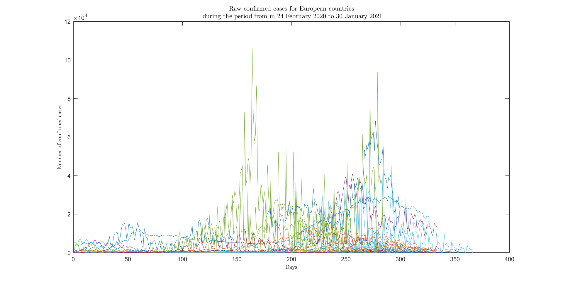
Figure 13: Confirmed cases: row data

2. Regular and persistent features, common to many countries with different levels of disease severity, highlight a general underlying dynamic of the spread of the disease. As for many countries, although with different social and geographical conditions, the presence of different peaks observed in the curve of confirmed cases (Fig.13) suggests to model the disease spread by multiple waves of infection, considering each of them as a single independent infection process. We concentrated our analysis on the two biggest waves observed in most of the considered countries.

3. We applied this multiple waves scheme describing each of the two waves by a single uni-modal distribution. In order to separate dataset of each country we selected time intervals around the two highest peaks, whose endpoints coincide with the lowest values before and after a peak. For practical calculation, we assume these values represent respectively the onset and the close of a single wave of infection although in many cases the there is an overlap between consecutive waves.

4. We restricted our analysis excluding abrupt change in dynamical conditions, and applying our procedures to consecutive waves of infection. In other words, we assume the pandemic, after a finite time interval, has exhausted its actual pathogenic load, due to natural causes or to containment rules adopted. This allows us to deal with asymptotic quantities in the limit of large time $t$.

5. We denote by $c_{n,i}^{g,\nu}$ and $s_{n,i}^{g,\nu}$ observations related respectively to the $n$-th daily number of confirmed case and $n$-th daily number of performed diagnostic test for the $i$-th European country ($g=E$ and $i=1,...,37$ ) or for the $i$-th Italian region ($g=I$ and $i=1,...,21$) during the first ($\nu=1$) or second ($\nu=2$) wave of infection.Identifying the white balls with the variable $c_{n,i}^{g,\nu}$ and the number of drawn balls, at each step $n$, with the daily tests $s_{n,i}^{g,\nu}$, we describe the infection spread by a Polya process, assuming that each time series $c_{n,i}^{g,\nu}$ follows a Negative Binomial distribution $N\!B(r_{i}^{g,\nu},p_{i}^{g,\nu})$, with parameters $r_{i}^{g,\nu}$ and $p_{i}^{g,\nu}$ defined as above for each $i$, $g$ and $\nu$.

6. We applied our procedure separately to the set of national data and to the regional one so as to analyse and compare the spreading of COVID-19 at different scales in terms of number of population and geographical size. We repeated the procedure for the first and the second wave of infection.

7. Based on the assumption 2, we assumed that, for each wave of infection, the group of European countries was approximately in the same local conditions: actually they have approximately the same initial ratio between infected and susceptible cases ($\rho_{0,i}^{E,\nu}\simeq\rho_{0}^{E,\nu}$), and the same normalized reproduction number ($\delta_{i}^{E,\nu}\simeq\delta^{E,\nu}$), independently from the $i$-th considered country. This implies that, for large $n$, since we can rewrite $r_{i}^{E,\nu}\equiv\frac{\rho_{0,i}^{E,\nu}}{\delta_{i}^{E,\nu}}$, and $p_{i}^{g,\nu}\equiv\frac{1}{1+n\delta_{i}^{E,\nu}}$, also $r_{i}^{E,\nu}\simeq r^{E,\nu}\equiv\frac{\rho_{0}^{E,\nu}}{\delta^{E,\nu}}$ and $p_{i}^{E,\nu}\simeq p^{E,\nu}\equiv\frac{1}{1+n\delta^{E,\nu}}$. In order to account these conditions, we assumed that, at fixed $\nu$, the Negative Binomials of assumption 5 can be seen as Negative Binomial compound distributions $N\!B(r_{i}^{E,\nu},p_{i}^{E,\nu})$ in which the characteristic parameters are both normally distributed with a small variance, such that $r_{i}^{E,\nu}$ and $p_{i}^{E,\nu}$ can be approximated by their mean values: $r_{i}^{E,\nu}\simeq r^{E,\nu}$ and $p_{i}^{E,\nu}\simeq p^{E,\nu}$. Finally, for each wave of infection, European countries can be represented by independent urns, each of them containing a different total number of balls, corresponding to the different population, but providing the same Negative Binomial compound distribution $N\!B(r^{E,\nu},p^{E,\nu})$.

8. Let define $R_{n,i}^{E,\nu}\equiv\frac{\sum\limits_{t=1}^{n}c_{t,i}^{g,\nu}}{\sum\limits_{t=1}^{n}s_{t,i}^{g,\nu}}$ the ratio between cumulative cases and cumulative diagnostic tests. In our scheme each $R_{n,i}^{E,\nu}$ replaces the sample average $Z_{n,i}^{E,\nu}$ of eq.2 for each process. Inspired by general results [19, 20], we assume that each $R_{n,i}^{E,\nu}$ follows a Beta limiting distribution $B\big{(}r_{i}^{E,\nu},\theta_{i}^{E,\nu}\big{)}$. On the other hand, according to the assumption 7 they can reduce to the same $B\big{(}r^{E,\nu},\theta^{E,\nu}\big{)}$, since $\theta_{i}^{E,\nu}\simeq\theta^{E,\nu}\equiv\frac{1}{\delta^{E,\nu}}-r^{E,\nu}$.

9. The previous assumptions 7-8 were stated also at regional scale, considering data related to the group of the Italian regions with different population but with the same $\rho_{0}^{I,\nu}$ and the same $\delta^{I,\nu}$, for all $i$.

Assumption 7 is the hard hypothesis of our procedure and it will verified a-posteriori by succeeding results.

2.2 Infection rate estimation based on universality assumptions

For our calculations confirmed cases and diagnostic tests data of the 37 accessible European countries were collected from 24 February 2020 to 30 January 2021. Data have reported by Humanitarian Data Exchange (HDX) database [21], that provides national data worldwide. For the Italian case, we consider all the 21 regions using data provided by the Italian Civil Protection Agency (CPA) database [22] on daily time scales. Under the above assumptions we fitted the $N\!B(r_{i}^{g,\nu},p_{i}^{g,\nu})$ PDFs for each of the 37 European selected countries and for each of the 21 Italian regions. For properly selecting observations for each wave of infection and for each country, we proceeded as described in assumption 3. In most of the countries, a multiple waves path is recognizable from daily confirmed cases curve. Although shifted by a time delay, all confirmed cases curves show a first isolated wave followed by a second or a third big wave overlapping each other and a number of smaller peaks that seem to be not ascribable to random fluctuations. We consider only the two biggest waves, locating the onset and close points simply considering the minima around each peak. The maximum likelihood estimation algorithm was used to compute the fitting parameters $r_{i}^{g,\nu}$ and $p_{i}^{g,\nu}$ . For practical calculation, we adopted the fitdist function implemented in Matlab, training the models with the confirmed cases data $c_{n,i}^{g,\nu}$. In order to select PDFs that successfully fit confirmed cases data, we performed both Kolmogorov-Smirnov (KS-test) and Chi-square test ($\chi^{2}$-test) using respectively the kstest and the chi2gof Matlab functions. As a result, over both the two waves, we were able to select a subset of European countries (about $74\%$ of successful PDFs) and a subset of Italian regions(about $64\%$ of successful PDFs) that passed both the tests. To assess the validity of our procedure we must to justify the assumption 7. To this aim, we first computed sample means and variances of the estimated parameters $r_{i}^{g,\nu}$ ($\mu_{r}^{g,\nu}$ and $\sigma_{r}^{g,\nu}$ ) and $p_{i}^{g,\nu}$ ( $\mu_{p}^{g,\nu}$ and $\sigma_{p}^{g,\nu}$), then, under normality assumption we statistically tested whether each variance $\sigma_{*}^{g,\nu}$ was significantly different from zero. A t-test was performed for each $\sigma_{*}^{g,\nu}$, using ttest Matlab function. Successful results, from all of the performed tests, allow us to approximate $r_{i}^{g,\nu}$ and $p_{i}^{g,\nu}$, according to assumption 7 and accounting for universality stated in assumption 2 and 7. Once the distributions of confirmed cases have been proved, the problem of estimating the asymptotic value $\rho_{\infty}$ reduces to compute the mean of the asymptotic distributions $B\big{(}r^{g,\nu},\theta^{g,\nu}\big{)}$. In fact, according to assumption 8, for each waves, we can consider data from each European country, or Italian region, as $i$ different sequences of trials of a process with different population but characterized by the same Beta PDF. This implies that, for each group $g$ and for each wave of infection $\nu$, we can assume $R_{n,i}^{g,\nu}$ are governed by the same $B\big{(}r^{g,\nu},\theta^{g,\nu}\big{)}$. As a result we were able to fit the four Beta PDFs by using the set of the $i$ limiting values $R_{\infty,i}^{g,\nu}=\lim_{n\to\infty}R_{n,i}^{g,\nu}$ (see Fig.14-15). A cut-off value has been also introduced to establish a finite size convergence criterion. However, in most of the cases $R_{\infty,i}^{g,\nu}$ were obtained directly by the ratio computed on the end points of each waves of infection, since they can be considered far enough to represent the limit for large times, where the stability of $R_{n,i}^{g,\nu}$ is reached. Also in this case, maximum likelihood estimation algorithm and fitdist function was adopted to estimate the parameters $r^{g,\nu}$ and $\theta^{g,\nu}$, for each Beta PDFs. KS-test and $\chi^{2}$-test were also successfully conducted to assess the performance of the estimated Beta. In order to assure the consistency of the whole procedure we tested whether each $r^{g,\nu}$, estimated by $B\big{(}r^{g,\nu},\theta^{g,\nu}\big{)}$, was significantly different from respective $\mu_{r}^{g,\nu}$ estimated by $N\!B(r_{i}^{g,\nu},p_{i}^{g,\nu})$. For each group $g$ and each wave of infection $\nu$ we implement a one-sample two tailed t-test, under the null hypothesis $\mu_{r}^{g,\nu}=r^{g,\nu}$. A two-sample two tailed t-test to simultaneously compare couples of $\mu_{r}^{g,\nu}$ with crossed $g$ and $\nu$ suggesting the invariance of $r^{g,\nu}$ under change of $\nu$ or $g$ and similarity behaviour at different scales. Finally an estimation of the mean value $\rho_{\infty}^{g,\nu}$ was obtained. All results are provided in the next sessions.

3 Results

3.1 European countries

For our calculation we restricted to the countries with total population grater than one million, selecting 40 of the 48 countries from European continent, reported in the HDX database (see Tab.1-2). We also discarded countries that did not provide diagnostic test data at all (Albania, Montenegro, Moldova). We preprocessed remaining 37 European countries, first removing inconsistent data (outliers and negative data) than selecting only observations corresponding to performed diagnostic tests. Wherever possible, data were collected on daily time scale, otherwise we smoothed weekly data, $c_{n,i}^{g,\nu}$ and $s_{n,i}^{g,\nu}$, as in the case of Germany, Spain, Netherlands, France and Ukraine. Due to different starting day of the pandemic, delays or corruptions in data reporting, four countries (Bulgaria, Cyprus, Czechia, North Macedonia ) did not provided sufficient data for the first wave of infection. As a result, we obtain two sets composed by 33 countries for the first wave and by 37 for the second wave. Fitting procedures were applied on the above two groups and both KS-test and $\chi^{2}$-test with a confidence level $\alpha=0.01$, were performed to select successful PDFs, whose p-values were reported in Tab.1-2. Resulting $i=27$ successful $N\!B(r_{i}^{E,1},p_{i}^{E,1})$ PDFs for the first wave are showed in Fig.1-3, where we reported fitted PDFs (Fig.1) and their relative CDFs (Fig.2-3). The same procedures were performed for the second wave (Fig.4-6) obtaining $i=28$ successful $N\!B(r_{i}^{E,2},p_{i}^{E,2})$. Fitting parameters $r_{i}^{E,\nu}$ and $p_{i}^{E,\nu}$ of all successful PDFs were reported in Tab.1-2 (first wave) and Tab.4-5 (second wave). In Fig.2-3 and Fig.5-6, is also reported the graphical comparison between fitted CDFs and empirical distribution functions, computed with a $95\%$ confidence interval ($\%$ c.i.). By using the successful subset of data we computed sample means and variances ($\mu_{r}^{E,\nu}$, $\sigma_{r}^{E,\nu}$ and $\mu_{p}^{E,\nu}$, $\sigma_{p}^{E,\nu}$). Excluding the two outliers values coming from Ukraine and Poland, for the first wave, we obtained $\mu_{r}^{E,1}=1.48$ ($95\%$ c.i.: $1.34-1.62$) and $\mu_{p}^{E,1}=3.17\cdot 10^{-2}$ ($95\%$ c.i.: $2.06\cdot 10^{-2}-4.28\cdot 10^{-2}$) (see Tab.3). Similar results were obtained for the second wave: $\mu_{r}^{E,2}=1.68$ ($95\%$ c.i.: $1.54-1.82$) and $\mu_{p}^{E,2}=0.04\cdot 10^{-2}$ ($95\%$ c.i.: $0.03\cdot 10^{-2}-0.05\cdot 10^{-2}$). For each wave of infection we assessed the sharpness of the normal distributions $r_{i}^{E,\nu}$ and $p_{i}^{E,\nu}0$ by using two one-sample two-tailed t-tests, with a significance level $\alpha=0.05$, under the null hypothesis that respectively $\sigma_{r}^{E,\nu}=0$ and $\sigma_{p}^{E,\nu}=0$. All tests were successful, with a p-values within the interval (0.08 - 0.6). Focusing on parameters $r_{i}^{E,\nu}$ we also note that $\mu_{r}^{E,1}$ is very closed to $\mu_{r}^{E,2}$ within the c.i., suggesting it is invariant also under change of the wave $\nu$ considered. In order to verify the latter hypothesis ($\mu_{r}^{E,1}=\mu_{r}^{E,2}$) a two-sample two-tailed t-test, with a significance level $\alpha=0.05$, was also performed with success, by using ttest2 function, and obtaining a p-value 0.09. On the contrary, concerning, the sample means $\mu_{p}^{E,\nu}$ they can’t directly compared with a target value since the parameters $p^{E,\nu}$ can’t be directly estimated from $B\big{(}r^{g,\nu},\theta^{g,\nu}\big{)}$. On the other hand, $\mu_{p}^{E,\nu}$ strongly decreases passing from the first wave to the second one. The deviation observed can be due by different values of $d$ trough $\delta^{E,\nu}$: increasing values of $\delta^{E,\nu}$ imply decreasing value of $p_{i}^{E,\nu}$ and of the relative sample means $\mu_{p}^{E,\nu}$. All these results support our assumptions (2 and 7-9) although a more detailed analysis is prevented since $\delta^{g,\nu}$ cannot be directly estimated from $p_{i}^{g,\nu}$ or $\theta^{g,\nu}$ . Once the convergence of $R_{n,i}^{E,\nu}$ was reached, for each selected country, asymptotic values of the ratio $R_{\infty,i}^{E,\nu}$ were used to fit the two Beta PDFs $B\big{(}r^{E,\nu},\theta^{E,\nu}\big{)}$, (see Fig.7). KS-test and $\chi^{2}$-test were successfully performed on both the distributions. Fitting parameters $r^{E,\nu}$ and $\theta^{E,\nu}$ related to the Beta distributions were estimated and reported in Tab.3. We found a value of $1.80$ ($95\%$ c.i.: $1.07-3.02$) for $r^{E,1}$ and $1.95$ ($95\%$ c.i.: $1.10-3.46$) for $r^{E,2}$, showing that, within the c.i., $r^{E,\nu}$ are consistent with the sample means obtained from estimated Negative Binomials. In order to complete the comparison between parameters satisfying the initial condition in assumption 7-9, a two one-sample two-tailed t-tests were conducted, testing the null hypothesis that respectively $\mu_{r}^{E,1}=r^{E,1}$ and $\mu_{r}^{E,2}=r^{E,2}$. Both tests passed successfully with a p-value respectively equal to 0.6 and 0.1. Finally we computed expected values $\rho_{\infty}^{E,\nu}=\rho_{0}^{E,\nu}$ (Tab.3). We obtained a value $\rho_{\infty}^{E,1}=0.05$ ($95\%$ c.i.: $0.03-0.07$) for the first wave and $\rho_{\infty}^{E,2}=0.11$ ($95\%$ c.i.: $0.08-0.14$) for the second one. Both results seem in good agreement with the observations provided worldwide for the incidence rate on monthly scale [ECDC] and the deviation between the two values accounts for the observed growing of the incidence rate passing from the first to the second wave of infection. Moreover, since parameters $r^{E,1}$ and $r^{E,2}$ are very close the different values resulting from incidence rate estimations $\rho_{\infty}^{E,\nu}$, are mainly due by parameters $\theta^{E,\nu}$, which pass from $\theta^{E,1}=34.92$ ($95\%$ c.i.: $21.08-57.46$) for the first wave to $\theta^{E,1}12.86$ ($95\%$ c.i.: $6.07-27.02$) for the second one. A decreasing $\theta^{E,\nu}$ means an increasing $\delta^{E,\nu}$, which corresponds to an increasing $d$, the population number being constant. This could be explained by an increasing viral load, conceivably due to the inflow of a more aggressive variant of the virus, associated with an increasing initial sick population $w$, since the parameter $r^{E,\nu}$ is proved to remain constant varying $\nu$.

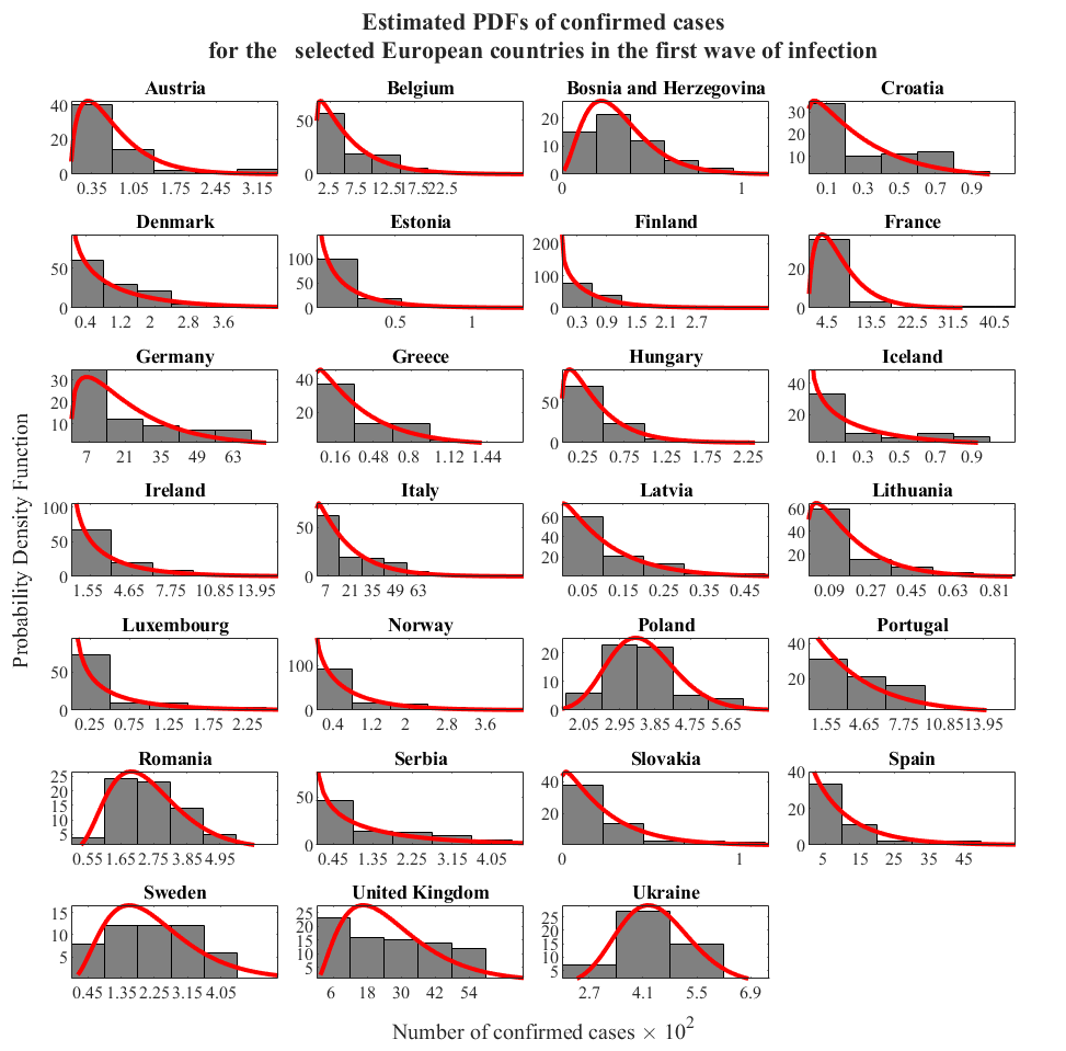
Figure 1: Negative Binomial PDFs (red line) of the confirmed cases; the group of 27 successful European countries, during the first waves of infection, was considered. Histograms of observed confirmed cases were also reported (bar plot). Black dashed lines represent upper and lower bounds, with $95\%$ c.i.

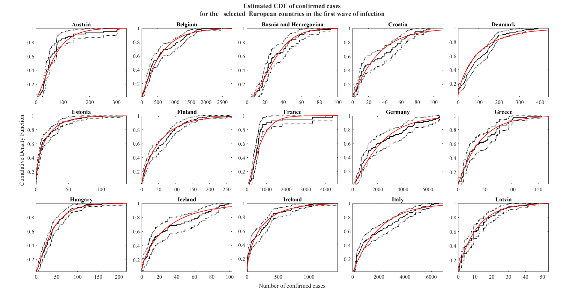
Figure 2: Negative Binomial CDFs (red line) of the confirmed cases; the group of 27 successful European countries, during the first waves of infection, was considered. Empirical CDFs of confirmed cases was reported (black line); black dashed lines represent upper and lower bounds, with $95\%$ c.i..

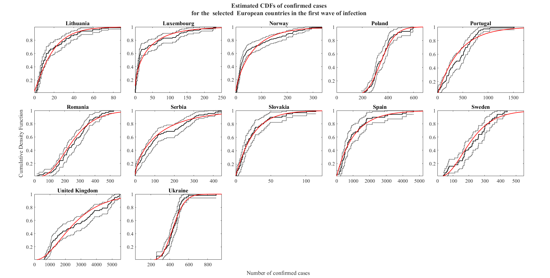
Figure 3: Negative Binomial CDFs (red line) of the confirmed cases; the group of 27 successful European countries, during the first waves of infection, was considered. Empirical CDFs of confirmed cases was reported (black line); black dashed lines represent upper and lower bounds, with $95\%$ c.i..

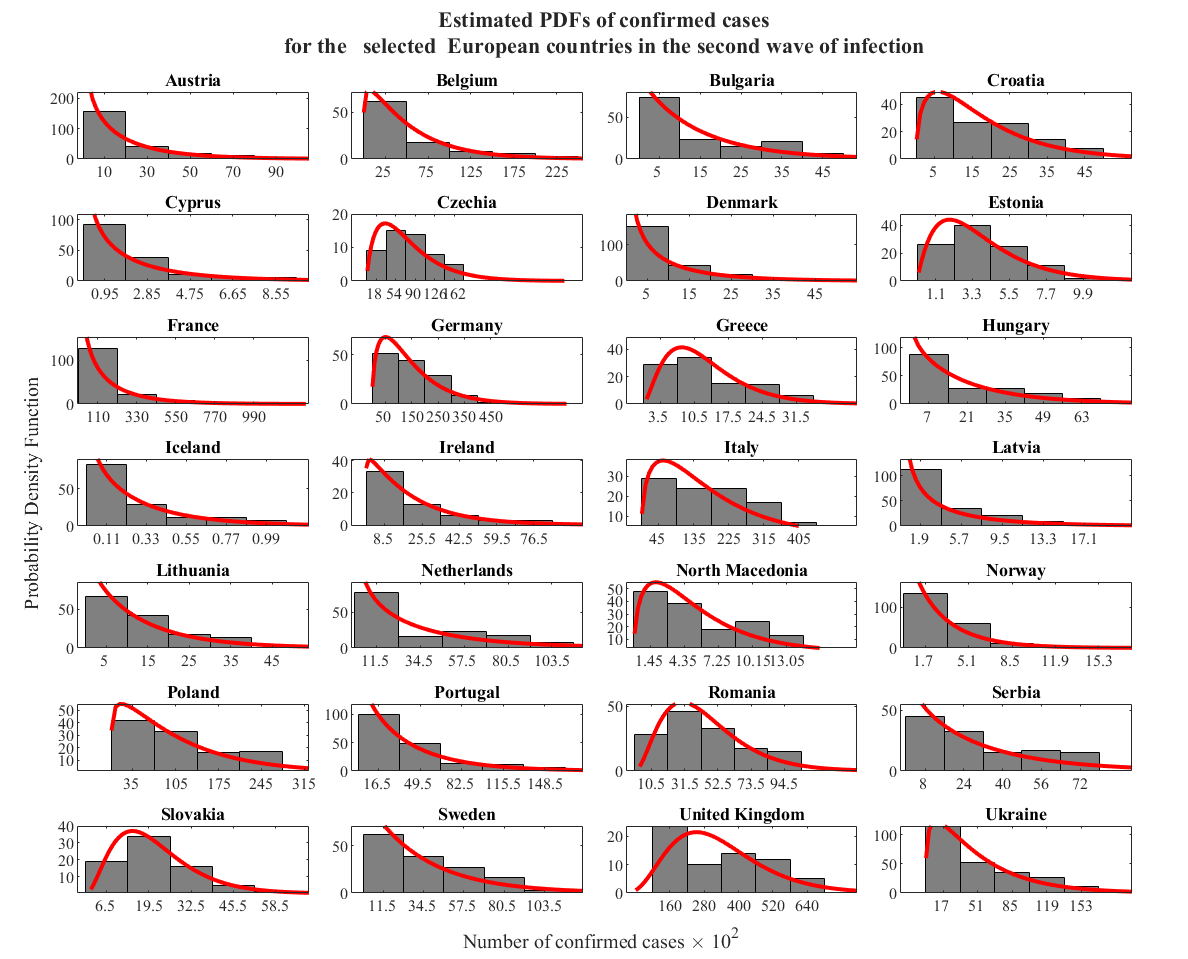
Figure 4: Negative Binomial PDFs (red line) of the confirmed cases; the group of 28 successful European countries, during the first waves of infection, was considered. Histograms of observed confirmed cases were also reported (bar plot). Black dashed lines represent upper and lower bounds, with $95\%$ c.i..

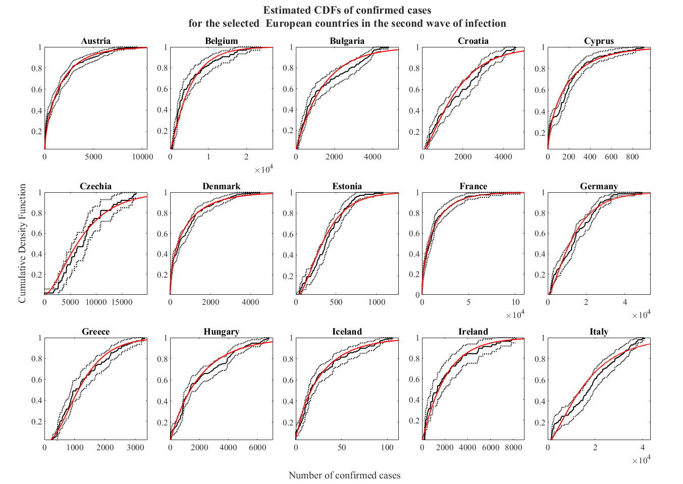
Figure 5: Negative Binomial CDFs (red line) of the confirmed cases; the group of 28 successful European countries, during the first waves of infection, was considered. Empirical CDFs of confirmed cases was reported (black line); black dashed lines represent upper and lower bounds, with $95\%$ c.i..

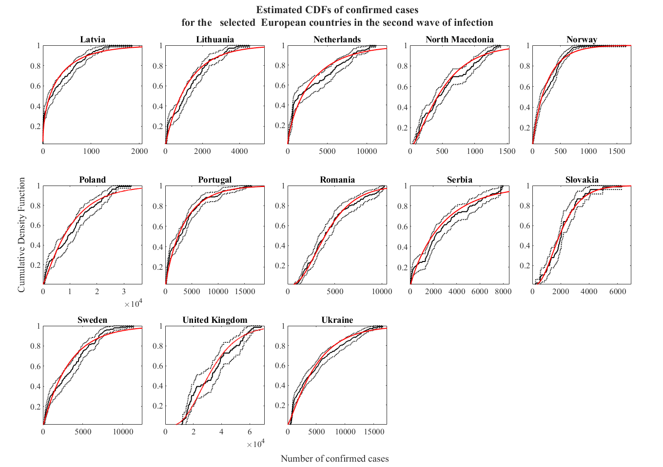
Figure 6: Negative Binomial CDFs (red line) of the confirmed cases; the group of 28 successful European countries, during the first waves of infection, was considered. Empirical CDFs of confirmed cases was reported (black line); black dashed lines represent upper and lower bounds, with $95\%$ c.i..

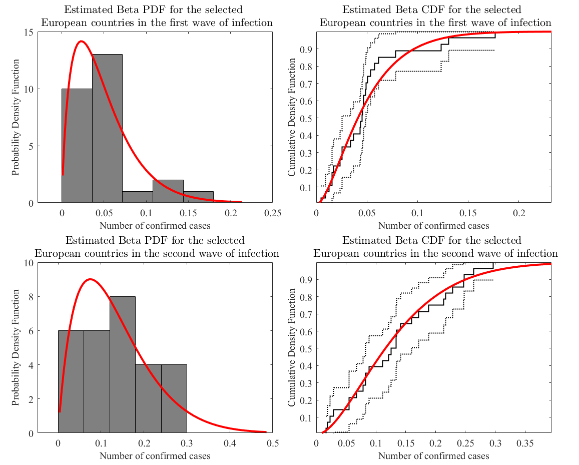
Figure 7: On the right: Beta PDFs of the ratio $R_{i,\infty}^{E,\nu}$ (red line) with relative histogram (bar plot) during the first (up) and second (down) waves of infection. On the left: CDFs corresponding to the above PDFs (red line); black dashed lines represent upper and lower bound, with $95\%$ c.i..

Countries	$\bm{r_{i}^{E,1}\pm 95\%\textbf{c.i.}}$	$\bm{p_{i}^{E,1}\pm 95\%\textbf{c.i.}}\;\bm{[10^{-2}]}$	$\bm{p-\textbf{value}}$
Austria	1.70 $\pm$ 0.57	2.33 $\pm$ 0.92	0.15
Belgium	1.11 $\pm$ 0.28	0.19 $\pm$ 0.06	0.54
Bos.-Herzeg.	3.29 $\pm$ 1.31	9.33 $\pm$ 3.62	0.72
Croatia	1.12 $\pm$ 0.36	3.44 $\pm$ 1.30	0.24
Denmark	0.70 $\pm$ 0.17	0.67 $\pm$ 0.22	0.02
Estonia	0.59 $\pm$ 0.14	3.59 $\pm$ 1.17	0.01
Finland	0.83 $\pm$ 0.19	1.48 $\pm$ 0.43	0.15
France	1.73 $\pm$ 0.70	0.25 $\pm$ 0.12	0.06
Germany	1.35 $\pm$ 0.40	0.06 $\pm$ 0.03	0.22
Greece	1.06 $\pm$ 0.35	2.57 $\pm$ 1.02	0.49
Hungary	1.30 $\pm$ 0.35	3.12 $\pm$ 0.97	0.70
Iceland	0.69 $\pm$ 0.24	2.34 $\pm$ 1.04	0.66
Ireland	0.62 $\pm$ 0.14	0.26 $\pm$ 0.09	0.38
Italy	1.04 $\pm$ 0.23	0.06 $\pm$ 0.02	0.12
Latvia	1.08 $\pm$ 0.32	8.98 $\pm$ 2.94	0.44
Lithuania	1.27 $\pm$ 0.36	6.55 $\pm$ 2.11	0.08
Luxembourg	0.50 $\pm$ 0.12	1.24 $\pm$ 0.46	0.01
Norway	0.77 $\pm$ 0.16	1.11 $\pm$ 0.33	0.01
Poland	17.57 $\pm$ 6.53	4.74 $\pm$ 1.69	0.66
Portugal	1.02 $\pm$ 0.32	0.25 $\pm$ 0.10	0.06
Romania	4.20 $\pm$ 1.38	1.59 $\pm$ 0.55	0.71
Serbia	0.62 $\pm$ 0.17	0.49 $\pm$ 0.19	0.29
Slovakia	1.10 $\pm$ 0.39	4.41 $\pm$ 1.82	0.87
Spain	0.94 $\pm$ 0.34	0.09 $\pm$ 0.05	0.32
Sweden	3.32 $\pm$ 1.27	1.46 $\pm$ 0.59	0.56
Un.Kingdom	2.57 $\pm$ 0.75	0.15 $\pm$ 0.04	0.23
Ukraine	22.04 $\pm$ 9.01	4.73 $\pm$ 1.87	0.73

Table 1: Fitting parameters $r_{i}^{E,1}$ and $p_{i}^{E,1}$ of the Negative Binomial PDFs for the selected European countries, in the first wave of infection. Best p-values resulting from both KS and $\chi^{2}$ test are also reported.

Countries	$\bm{r_{i}^{E,2}\pm 95\%\textbf{c.i.}}$	$\bm{p_{i}^{E,2}\pm 95\%\textbf{c.i.}}\;[10^{-2}]$	$\bm{p-\textbf{value}}$
Austria	0.67 $\pm$ 0.10	0.04 $\pm$ 0.01	0.04
Belgium	1.13 $\pm$ 0.28	0.03 $\pm$ 0.01	0.14
Bulgaria	0.97 $\pm$ 0.20	0.07 $\pm$ 0.02	0.30
Croatia	1.48 $\pm$ 0.34	0.09 $\pm$ 0.03	0.12
Cyprus	0.59 $\pm$ 0.12	0.31 $\pm$ 0.09	0.01
Czechia	1.79 $\pm$ 0.67	0.03 $\pm$ 0.01	0.51
Denmark	0.51 $\pm$ 0.08	0.07 $\pm$ 0.02	0.12
Estonia	2.03 $\pm$ 0.52	0.53 $\pm$ 0.16	0.13
France	0.58 $\pm$ 0.10	0.01 $\pm$ 0.01	0.77
Germany	1.54 $\pm$ 0.33	0.02 $\pm$ 0.01	0.14
Greece	2.57 $\pm$ 0.68	0.20 $\pm$ 0.06	0.34
Hungary	0.88 $\pm$ 0.16	0.05 $\pm$ 0.02	0.18
Iceland	0.77 $\pm$ 0.18	2.77 $\pm$ 0.82	0.15
Ireland	1.06 $\pm$ 0.34	0.06 $\pm$ 0.03	0.70
Italy	1.47 $\pm$ 0.37	0.01 $\pm$ 0.01	0.05
Latvia	0.46 $\pm$ 0.08	0.14 $\pm$ 0.04	0.04
Lithuania	0.90 $\pm$ 0.18	0.08 $\pm$ 0.02	0.10
Netherlands	0.72 $\pm$ 0.14	0.03 $\pm$ 0.01	0.02
Nor.Maced.	1.53 $\pm$ 0.32	0.29 $\pm$ 0.08	0.11
Norway	0.87 $\pm$ 0.15	0.34 $\pm$ 0.08	0.04
Poland	1.17 $\pm$ 0.27	0.02 $\pm$ 0.01	0.18
Portugal	0.87 $\pm$ 0.15	0.03 $\pm$ 0.01	0.06
Romania	3.02 $\pm$ 0.67	0.07 $\pm$ 0.02	0.90
Serbia	0.87 $\pm$ 0.19	0.04 $\pm$ 0.01	0.01
Slovakia	3.04 $\pm$ 0.92	0.15 $\pm$ 0.05	0.33
Sweden	1.01 $\pm$ 0.20	0.04 $\pm$ 0.01	0.05
Un.Kingdom	4.13 $\pm$ 1.35	0.02 $\pm$ 0.01	0.27
Ukraine	1.25 $\pm$ 0.20	0.03 $\pm$ 0.01	0.02

Table 2: Fitting parameters $r_{i}^{E,2}$ and $p_{i}^{E,2}$ of the Negative Binomial PDFs for the selected European countries, in the second wave of infection. Best p-values resulting from both KS and $\chi^{2}$ test are also reported.

Waves of
infection
(W.I-II)		$\bm{r^{E,\nu}\;(95\%\textbf{c.i.})}$	$\bm{\theta^{E,\nu}\;(95\%\textbf{c.i.})}$	$\bm{\rho_{\infty}^{E,\nu}\;(95\%\textbf{c.i.})}$	$\mu_{r}^{E,\nu}\;(95\%$ c.i.)	$\mu_{p}^{E,\nu}\;(95\%$ c.i.)$[10^{-2}]$
W.I		$1.80\;(1.07-3.02)$	34.92 $(21.08-57.46)$	$0.05\;(0.03-0.07)$	$1.48$ ( $1.34-1.62$)	$3.17$ ($2.06-4.28$)
W.II		$1.95\;(1.10-3.46)$	$12.86\;(6.07-27.02)$	$0.11\;(0.08-0.14)$	1.68 ( $1.54-1.82$)	0.04 ($0.03-0.05$)

Table 3: Fitting parameters $r^{E,\nu}$ and $\theta^{E,\nu}$ of the Beta PDFs for the first and second waves of infection. Mean values $\rho_{\infty}^{E,\nu}$ and p-values, resulting from both KS and $\chi^{2}$ test, are also reported.

3.2 Italy

The entire procedure described above for the European case was repeated for the 21 Italian regions, in particular the sequence of statistical tests with the same significance levels. Fig.8-11 show 14 and 13 successful Negative Binomials PDFs and CDFs, corresponding to the selected regions during respectively the first and the second wave of infection. Tab.4-5 report the estimated fitting parameters, for both the two waves. Sample means and variance of $r^{I,\nu}$ and $p^{I,\nu}$ were estimated obtaining the following results: $\mu_{r}^{I,1}=0.52$ $95\%$ c.i. $(0.39-0.65)$, $\mu_{p}^{I,1}=1.11$ $95\%$ c.i. $(0.81-1.41)$, $\mu_{r}^{I,2}=0.45$ $95\%$ c.i. $(0.37-0.53)$ and $\mu_{p}^{I,2}=0.12$ $95\%$ c.i. $(0.07-0.17)$. An analogue sequence of one-sample two-tailed t-tests on both the variances were successfully performed. Two one-sample two-tailed t-tests for comparing $\mu_{*}^{I,1}$ and $\mu_{*}^{I,2}$ were also successfully performed. Results seem internally consistent and consistent with the European scenario. However, parameters $r^{I,\nu}$ and $\theta^{I,\nu}$, estimated by the $B\big{(}r^{I,\nu},\theta^{I,\nu}\big{)}$, show some deviation from European case that need to be discussed. In fact, while $r^{I,1}$ value can be still considered in agreement with previous results, $r^{I,2}$ is clearly far from all respective value changing $g$ or $\nu$. Nevertheless, a look to the Tab.6 shows that values of $\rho_{\infty}^{I,1}=0.04$ $95\%$ c.i. $(0.02-0.06)$ and $\rho_{\infty}^{I,2}=0.07$ $95\%$ c.i. $(0.05-0.09)$ seems in agreement respectively with the first and second waves related to the European case. Actually the reason why the strong differences between values of $r^{I,2}$ estimated from the corresponding Beta and the mean values of $r_{i}^{I,2}$ obtained from the single regions, must be sought in that a small amount of data are available. Moreover, similarly to the European case (Fig.15), in the second wave the ratio $R_{i,n}^{I,2}$ have not reached yet stable values. Crossed t-tests, as described in the European case were also performed comparing all corresponding Italian and European estimated parameters with successful results.

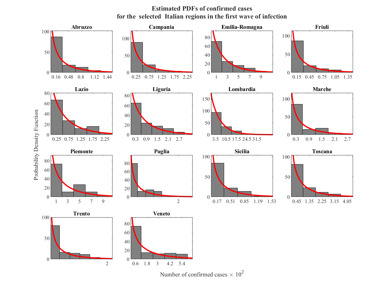
Figure 8: Negative Binomial PDFs (red line) of the confirmed cases; the group of 14 successful Italian regions, during the first waves of infection, was considered. Histograms of observed confirmed cases were also reported (bar plot). Black dashed lines represent upper and lower bounds, with $95\%$ c.i..

Figure 9: Negative Binomial CDFs (red line) of the confirmed cases; the group of 14 successful Italian regions, during the first waves of infection, was considered. Empirical CDFs of confirmed cases was reported (black line); black dashed lines represent upper and lower bounds, with $95\%$ c.i..

Figure 10: Negative Binomial PDFs (red line) of the confirmed cases; the group of 13 successful Italian regions, during the first waves of infection, was considered. Histograms of observed confirmed cases were also reported (bar plot). Black dashed lines represent upper and lower bounds, with $95\%$ c.i..

Figure 11: Negative Binomial CDFs (red line) of the confirmed cases; the group of 13 successful Italian regions, during the first waves of infection, was considered. Empirical CDFs of confirmed cases was reported (black line); black dashed lines represent upper and lower bounds, with $95\%$ c.i..

Figure 12: On the right: Beta PDFs of the ratio $R_{i,\infty}^{I,\nu}$ (red line) with relative histogram (bar plot) during the first (up) and second (down) waves of infection. On the left: CDFs corresponding to the above PDFs (red line); black dashed lines represent upper and lower bound, with $95\%$ c.i..

Countries	$\bm{r_{i}^{I,1}\pm 95\%\textbf{c.i.}}$	$\bm{p_{i}^{I,1}\pm 95\%\textbf{c.i.}\;[10^{-2}]}$	$\bm{p-\textbf{value}}$
Abruzzo	0.48 $\pm$ 0.11	1.78 $\pm$ 0.61	0.01
Campania	0.52 $\pm$ 0.12	1.32 $\pm$ 0.44	0.12
Emilia-Romagna	0.82 $\pm$ 0.18	0.37 $\pm$ 0.11	0.02
Friuli	0.51 $\pm$ 0.12	1.89 $\pm$ 0.64	0.03
Lazio	0.84 $\pm$ 0.19	1.29 $\pm$ 0.39	0.29
Liguria	0.81 $\pm$ 0.18	1.01 $\pm$ 0.30	0.11
Lombardia	0.99 $\pm$ 0.20	0.16 $\pm$ 0.04	0.19
Marche	0.50 $\pm$ 0.11	0.91 $\pm$ 0.31	0.14
Piemonte	0.65 $\pm$ 0.14	0.26 $\pm$ 0.08	0.03
Puglia	0.44 $\pm$ 0.10	1.21 $\pm$ 0.43	0.02
Sicilia	0.47 $\pm$ 0.11	1.68 $\pm$ 0.58	0.01
Toscana	0.54 $\pm$ 0.12	0.66 $\pm$ 0.21	0.16
Trento	0.41 $\pm$ 0.10	1.14 $\pm$ 0.41	0.01
Veneto	0.54 $\pm$ 0.11	0.35 $\pm$ 0.12	0.13

Table 4: Fitting parameters $r_{i}^{I,1}$ and $p_{i}^{I,1}$ of the Negative Binomial PDFs for the selected Italian regions, in the second wave of infection. Best p-values resulting from both KS and $\chi^{2}$ test are also reported.

Countries	$\bm{r_{i}^{I,2}\pm 95\%\textbf{c.i.}}$	$\bm{p_{i}^{I,2}\pm 95\%\textbf{c.i.}\;[10^{-2}]}$	$\bm{p-\textbf{value}}$
Abruzzo	0.39 $\pm$ 0.07	0.23 $\pm$ 0.07	0.02
Bolzano	0.40 $\pm$ 0.07	0.28 $\pm$ 0.08	0.01
Calabria	0.38 $\pm$ 0.07	0.34 $\pm$ 0.10	0.02
Campania	0.40 $\pm$ 0.07	0.04 $\pm$ 0.02	0.19
Lazio	0.50 $\pm$ 0.09	0.07 $\pm$ 0.02	0.01
Liguria	0.51 $\pm$ 0.09	0.19 $\pm$ 0.06	0.36
Lombardia	0.66 $\pm$ 0.11	0.03 $\pm$ 0.01	0.01
Piemonte	0.49 $\pm$ 0.07	0.06 $\pm$ 0.02	0.02
Sardegna	0.57 $\pm$ 0.10	0.34 $\pm$ 0.09	0.01
Sicilia	0.41 $\pm$ 0.07	0.09 $\pm$ 0.03	0.02
Toscana	0.42 $\pm$ 0.07	0.08 $\pm$ 0.03	0.02
Umbria	0.35 $\pm$ 0.07	0.24 $\pm$ 0.08	0.01
Veneto	0.53 $\pm$ 0.08	0.05 $\pm$ 0.01	0.01

Table 5: Fitting parameters $r_{i}^{I,2}$ and $p_{i}^{I,2}$ of the Negative Binomial PDFs for the selected Italian regions, in the second wave of infection. Best p-values resulting from both KS and $\chi^{2}$ test are also reported.

Waves of infection (W.I-II)		$\bm{r^{I,\nu}\;(95\%\textbf{c.i.})}$	$\bm{\theta^{I,\nu}\;(95\%\textbf{c.i.})}$	$\bm{\rho_{\infty}^{I,\nu}\;(95\%\textbf{c.i.})}$	$\bm{p-\textbf{value}}$
W.I		$2.85\;(1.01-6.10)$	$68.13\;(30.31-112.02)$	$0.04\;(0.02-0.06)$	0.82
W.II		$21.81\;(11.32-39.12)$	$273.82\;(115.04-401.10)$	$0.07\;(0.05-0.09)$	0.98

Table 6: Fitting parameters $r^{I,\nu}$ and $\theta^{I,\nu}$ of the Beta PDFs for the first and second waves of infection. Mean values $\rho_{\infty}^{I,\nu}$ and p-values, resulting from both KS and $\chi^{2}$ test, are also reported.

4 Conclusion

Guided by heuristic evidence of some universality property, here we propose to describe the spread of (SARS-CoV-2)-infected pneumonia (COVID-19) within a probabilistic Polya urn scheme. Under general homogeneity assumptions on initial conditions and applying a multiple waves approach, we analysed European data reported on confirmed cases and diagnostic test performed. A comparative analysis at regional and national scales was performed showing the presence of distinctive features according to the same underlying process at different scales. general characteristics can be extracted. Specific patterns and key indicators slightly depend from social or geographical conditions. On the other hand some parameter seem to hold universality properties, properly identifying COVID-19 infection. A sequence of statistical tests were performed to prove our hypothesis. Based on test results, for each wave of infection, we were able to consider data from each European country, or Italian region, as $i$ different sequences of trials of a process with different population but characterized by the same distribution for its sample average. This allows us to estimate the incidence rate $\rho_{\infty}$ by the asymptotic mean of the sample average of the process. Resulting estimation of $\rho_{\infty}^{g,\nu}$, related to the first and second wave of infection for the Italian case are broadly in line with European one and in agreement with real observations [23].

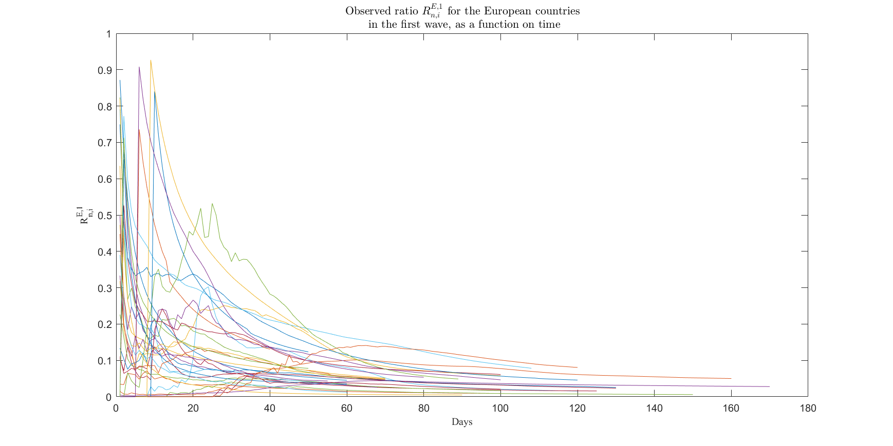
Figure 14:

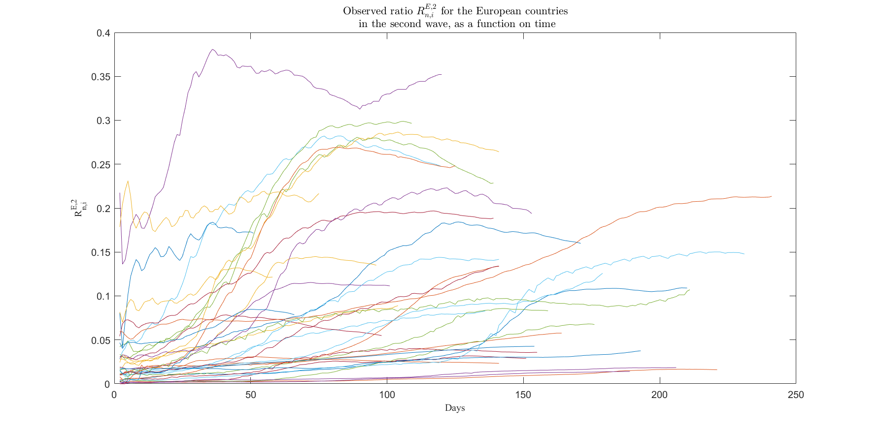
Figure 15:

5 Acknowledgement

The author would like to thank Dr. Maurizio Crippa for helpful discussion about insight of the present paper, and R. Gioia, C.E.O of H-DATA S.r.l.s. for technical support for the graphical elaborations.

References

- [1] World Health Organization. Report of the who-china joint mission on coronavirus disease 2019.
- [2] J. Papenburg, M. Baz, M. E. Hamelin et al., “Household transmission of the 2009 pandemic A/H1N1 influenza virus: elevated laboratory-confirmed secondary attack rates and evidence of asymptomatic infections”, Clinical Infectious Diseases, vol. 51, no. 9, pp. 1033–1041, (2010).
- [3] B. J. Cowling, S. Ng, E. S. K. Ma et al., “Protective efficacy of seasonal influenza vaccination against seasonal and pandemic influenza virus infection during 2009 in Hong Kong”, Clinical Infectious Diseases, vol. 51, no. 12, pp. 1370–1379, (2010).
- [4] ] J. Ma and P. Van Den Driessche, “Case fatality proportion”, Bulletin of Mathematical Biology, vol. 70, no. 1, pp.118–133, (2008).
- [5] H. Nishiura, “Case fatality ratio of pandemic influenza”, Lancet. Infect. Dis., vol. 10, no. 7, pp. 443–444, (2010).
- [6] S. N. Wood, E. C. Wit, M. Fasiolo, P. J. Green, “COVID-19 and the difficulty of inferring epidemiological parameters from clinical data”, Lancet. Infect. Dis., (2020).
- [7] T. W. Russell , J. Hellewell , C. I. Jarvis, et al., “Estimating the infection and case fatality ratio for coronavirus disease (COVID-19) using age-adjusted data from the outbreak on the Diamond Princess cruise ship, February 2020”, Euro Surveill. (2020).
- [8] R. Verity, L. C. Okell, I. Dorigatti et al., “Estimates of the severity of coronavirus disease 2019: a model-based analysis”, Lancet Infect. Dis. 2020; vol. 20, no. 6, pp. 669-677, (2020).
- [9] N. M. Ferguson et al., “Impact of non-pharmaceutical interventions (NPIs) to reduce COVID-19 mortality and healthcare demand”, Imperial College COVID-19 Response Team, (2020).
- [10] J. O. Lloyd-Smith, S. J. Schreiber, P. E. Kopp, and W. M. Getz, “Superspreading and the effect of individual variation on disease emergence”, Nature, 438, pp. 355–359, (2005).
- [11] M. Hayhoe, F. Alajaji and B. Gharesifard, “A Polya Contagion Model for Networks” in IEEE Transactions on Control of Network Systems, vol. 5, no. 4, pp. 1998-2010, (2018).
- [12] G. Polya, “Sur quelques points de la théorie des probabilités,” Annales de l’institut Henri Poincaré, vol. 1, no. 2, pp. 117–161, (1930).
- [13] F. Eggenberger and G. Polya, “ Über die statistik verketteter vorgänge,” Z. Angew. Math. Mech., vol. 3, no. 4, pp. 279–289, (1923).
- [14] M. Lipsitch, S. Riley, S. Cauchemez, A. C. Ghani, and N. M. Ferguson, “Managing and reducing uncertainty in an emerging influenza pandemic”, New England Journal of Medicine, vol. 361, no. 2, pp. 112–115, (2009).
- [15] K. Teerapabolarn, “An improved bound for negative binomial approximation with z-functions”, AKCE International Journal of Graphs and Combinatorics, 14:3, 287-294, (2017).
- [16] W. Feller, “An Introduction to Probability Theory and Its Applications”, Vol. II, 2nd edn. John Wiley, New York (1971).
- [17] N. L. Johnson, and S. Kotz, “Urn Models and Their Application”, John Wiley, New York, (1977).
- [18] S. Kotz, and N. Balakrishnan, “Advances in urn models during the past two decades”, Advances in Combinatorial Methods and Applications to Probability and Statistics, Birkhiuser, Boston, MA, pp 203-207 (1997).
- [19] D. Aoudia and F. Perron, “A New Randomized Pólya Urn Model”, Applied Mathematics, Vol. 3 No. 12A, pp. 2118-2122, (2012).
- [20] M. Chen and C. Z. Wei, “A New Urn Model”, Journal of Applied Probability at JSTOR: Vol. 42, No. 4, pp. 964-976, (2005)
- [21] Humanitarian Data Exchange, website https://data.humdata.org/event/covid-19.
- [22] Italian Civil Protection Agency, website https://github.com/pcm-dpc/COVID-19.
- [23] European Centre for Disease Prevention and Control, website https://www.ecdc.europa.eu/en/cases-2019-ncov-eueea