Dark matter Extensions of electroweak Higgs sector

Experimental signatures of a new dark matter WIMP

Abstract

The WIMP proposed here yields the observed abundance of dark matter, and is consistent with the current limits from direct detection, indirect detection, and collider experiments, if its mass is $\sim 72$ GeV/$c^{2}$. It is also consistent with analyses of the gamma rays observed by Fermi-LAT from the Galactic center (and other sources), and of the antiprotons observed by AMS-02, in which the excesses are attributed to dark matter annihilation. These successes are shared by the inert doublet model (IDM), but the phenomenology is very different: The dark matter candidate of the IDM has first-order gauge couplings to other new particles, whereas the present candidate does not. In addition to indirect detection through annihilation products, it appears that the present particle can be observed in the most sensitive direct-detection and collider experiments currently being planned.

As is well–known, there are a vast number of hypothetical dark matter candidates, most of which do not have well-defined masses or couplings, and many of which have already been ruled out by experiment. The most popular single candidate has been the lightest neutralino $\chi^{0}$ of supersymmetry (susy) [1]. But, as is also well-known, faith in this candidate has diminished during the past few years, because neither a susy dark matter WIMP nor other susy particles have been observed, despite strenuous efforts. In addition, the simplest susy models which have “natural” values for the parameters, and which are also compatible with limits from the LHC, are found to be in disagreement with both the abundance of dark matter and the limits from direct-detection experiments [2, 3, 4, 5, 6].

Here we propose an alternative candidate which in some respects resembles the neutralino, but which would open up a whole new sector with new particles and new physics which can be observed in the foreseeable future. We have named particles of this new kind “higgsons” [7, 8, 9, 10], represented by $H$, to distinguish them from Higgs bosons $h$ and the higgsinos $\widetilde{h}$ of susy. The lightest neutral particles in these three groups are $H^{0}$, $h^{0}$, and $\widetilde{h}^{0}$. We will demonstrate below that these new particles (higgsons) have very favorable features – after the theory has been reformulated in the way described below.

Many of these features are shared by the inert doublet model (IDM) – introduced long ago [11] and later proposed as an explanation of dark matter [12] – for which the phenomenology has been very extensively explored in many papers. Only a representative sample can be cited here [13, 14, 15, 16, 17, 18, 19, 20, 21, 22, 23, 24, 25, 26, 27], but the basic idea is that the Standard Model Higgs doublet is supplemented by a second doublet of scalar fields which have odd parity under a postulated new $Z_{2}$ symmetry. To avoid confusion, these fields will be distinguished by a subscript $I$:

$$\left(\begin{array}[]{c}H_{I}^{+}\\ \frac{1}{\sqrt{2}}\left(H_{I}^{0}+iA_{I}^{0}\right)\end{array}\right)\;.$$ (3)

Since each of these fields is odd with respect to the hypothetical $Z_{2}$, whereas all other fields are even, every term in the action must involve an even number of these fields. This makes the dark matter candidate $H_{I}^{0}$ stable, because it has the lowest mass. In addition, many of the successes described below for the present candidate, called $H^{0}$ here, are shared by $H_{I}^{0}$.

However, in the phenomenology of the IDM there are numerous important processes that involve first-order gauge couplings of $H_{I}^{0}$ to the other particles $A_{I}^{0}$ and $H_{I}^{\pm}$. See, e.g., Figs. 3 and 4 of [14]; Fig. 2 of [15]; Fig. 1 of [16]; Fig 4 of [18]; Figs. 9, 10, 11, 13, 14, 16, 17, 18, and 21 of [22]; Figs. 2 and 3 of [25]; Fig. 6 of [26]; Figs. 1 and 3 of [27]; and the constraints on the IDM parameters in Section 4.1 of [21], which imply that the masses of $A_{I}^{0}$ and $H_{I}^{\pm}$ should be reasonably near that of $H_{I}^{0}$.

As will be seen below, the present dark matter candidate $H^{0}$ has only second-order gauge couplings – and these are to only itself plus the gauge bosons. This results in a very different phenomenology, with a substantial reduction in the number of observable processes involved in annihilation, scattering, and creation. There are other differences: $H^{0}$ is its own antiparticle, it does not require an extra $Z_{2}$ symmetry, and it is related to Higgs bosons in a very different way.

We begin with the primitive 2-component spin 1/2 bosonic fields $\Phi_{r}$ introduced in our previous papers, which are joined in an $n$-component gauge multiplet $\widetilde{\Phi}_{r}$. (We name each multiplet $\widetilde{\Phi}_{r}$ after a typical member $\Phi_{r}$ in order to simplify the notation.) Each $\Phi_{r}$ transforms as a 2-component spinor under rotations, but is left unchanged by a boost.

It will be seen that the action for the physical fields $\Phi_{R}$, as defined below, is invariant under both rotations and boosts. The final theory is in fact fully Lorentz invariant.

For simplicity, we begin with a single (e.g. grand-unified) gauge field having covariant derivative

$$D_{\mu}=\partial_{\mu}-iA_{\mu}\quad,\quad A_{\mu}=A_{\mu}^{j}t^{j}$$ (4)

(so that the coupling constant is temporarily absorbed into $A_{\mu}$) and field strength

$$\quad F_{\mu\nu}=F_{\mu\nu}^{j}t^{j}\quad,\quad F_{\mu\nu}^{j}=\partial_{\mu}A_{\nu}^{j}-\partial_{\nu}A_{\mu}^{j}+c_{ii^{\prime}}^{j}A_{\mu}^{i}A_{\nu}^{i^{\prime}}\;.$$ (5)

Later we will specialize to the electroweak theory after symmetry breaking. Natural units $\hbar=c=1$ are used, with the $(-+++)$ convention for the metric tensor. Summations are never implied over a repeated gauge index like $r$ or $R$, but are always implied over repeated coordinate indices like $\mu,\nu=0,1,2,3$ and $k=1,2,3$, as well as the index $i$ or $j$ labeling gauge generators $t^{j}$. The same name and symbol are used for a field and the particle which is an excitation of that field.

The initial action for the new fields $\widetilde{\Phi}_{r}$ is

$$S_{r}=\int d^{4}x\,\widetilde{\Phi}_{r}^{{\dagger}}\left(x\right) D^{\mu}D_{\mu}\,\widetilde{\Phi}_{r}\left(x\right)$$

$$+\int d^{4}x\,\widetilde{\Phi}_{r}^{{\dagger}}\left(x\right)\,\overrightarrow{B}\left(x\right)\cdot\overrightarrow{\sigma}\;\widetilde{\Phi}_{r}\left(x\right)$$ (6)

where the 3-vectors $\overrightarrow{\sigma}$ and $\overrightarrow{B}$ respectively contain the Pauli matrices $\sigma^{k}$ and the “magnetic” components of the field strength tensor $F_{\mu\nu}$:

$$F_{kk^{\prime}}=-\varepsilon_{kk^{\prime}k^{\prime\prime}}B_{k^{\prime\prime}}\;.$$ (7)

(This action is derived in Ref. [7] but here is taken to be a phenomenological postulate [8].) At this point we deviate from our earlier papers by requiring all fundamental physical fields $\widetilde{\Phi}_{R}$ to satisfy Lorentz invariance. This means that the anomalous second term in (6) must disappear from the action. This can be achieved by requiring the physical fields to assume one of the two forms defined below, which are respectively called Higgs/amplitude fields and higgson fields.

Higgs/amplitude fields are defined to be those for which

$$\widetilde{\Phi}_{R}^{{\dagger}}\left(x\right)\,\overrightarrow{\sigma}\;\widetilde{\Phi}_{R}\left(x\right)=0$$ (8)

(where $\overrightarrow{\sigma}$ always implicitly multiplies an appropriate identity matrix). These fields – analogous to the Higgs/amplitude modes observed in superconductors [28] – are obtained by writing the $4n$-component $\widetilde{\Phi}_{R}$ in terms of $2n$-component fields $\widetilde{\Phi}_{r}$ and $\widetilde{\Phi}_{r^{\prime}}$ with opposite spins (and equal amplitudes):

$$\widetilde{\Phi}_{R}=\left(\begin{array}[]{c}\widetilde{\Phi}_{r}\\ \widetilde{\Phi}_{r^{\prime}}\end{array}\right)$$ (11)

so that

$$\widetilde{\Phi}_{R}^{{\dagger}}\left(x\right)\,\overrightarrow{\sigma}\,\widetilde{\Phi}_{R}\left(x\right) =\left(\begin{array}[]{cc}\widetilde{\Phi}_{r}^{{\dagger}}&\widetilde{\Phi}_{r^{\prime}}^{{\dagger}}\end{array}\right)\left(\begin{array}[]{cc}\overrightarrow{\sigma}&0\\ 0&\overrightarrow{\sigma}\end{array}\right)\left(\begin{array}[]{c}\widetilde{\Phi}_{r}\\ \widetilde{\Phi}_{r^{\prime}}\end{array}\right)$$ (17)

$$=\widetilde{\Phi}_{r}^{{\dagger}}\,\overrightarrow{\sigma}\,\widetilde{\Phi}_{r}+\widetilde{\Phi}_{r^{\prime}}^{{\dagger}}\,\overrightarrow{\sigma}\,\widetilde{\Phi}_{r^{\prime}}$$ (18)

$$=0\;.$$ (19)

In this case we write for each gauge component

$$\Phi_{R}\left(x\right)=\phi_{R}\left(x\right)\,\xi_{R}\quad\mathrm{\ with}\quad\xi_{R}^{\,{\dagger}}\,\xi_{R}=1$$ (20)

where $\xi_{R}$ has $4$ constant components and $\phi_{R}\left(x\right)$ is a $1$-component complex amplitude. Then (6) and its counterpart for $r^{\prime}$ reduce to

$$S_{R}=\int d^{4}x\,\mathcal{L}_{R}\quad,\quad\mathcal{L}_{R}=\widetilde{\phi}_{R}^{{\dagger}}\left(x\right)D^{\mu}D_{\mu}\,\widetilde{\phi}_{R}\left(x\right)$$ (21)

where $\widetilde{\phi}_{R}$ contains all the gauge components $\phi_{R}$.

In the electroweak theory, we interpret $\widetilde{\phi}_{R}$, with components $\phi_{R}^{0}$ and $\phi_{R}^{+}$, as the usual Higgs doublet (in the Higgs basis), with $\phi_{R}^{0}$ condensing and supporting Higgs boson excitations $h_{R}^{0}$:

$$\phi_{R}^{0}=v_{R}^{0}+h_{R}^{0}\quad,\quad v_{R}^{0}=\langle\phi_{R}^{0}\rangle\;.$$ (22)

We have assumed a pair of bosonic doublets $\widetilde{\Phi}_{r}$ and $\widetilde{\Phi}_{r^{\prime}}$ with the same gauge quantum numbers – i.e., (weak) isospin and hypercharge – in somewhat the same spirit as in standard susy. We choose the convention that $\widetilde{\Phi}_{r}$ has spin up and $\widetilde{\Phi}_{r^{\prime}}$ spin down for the field $\widetilde{\Phi}_{R}$ of (11) which condenses. There is then another independent field $\widetilde{\Phi}_{R^{\prime}}$ in which $\widetilde{\Phi}_{r}$ has spin down and $\widetilde{\Phi}_{r^{\prime}}$ spin up. This field has no condensate. Only the kinetic term of (6) has been treated at this point, without the potentially quite complicated terms that yield masses and further interactions.

Higgson fields are defined to be those for which

$$\Phi_{S}^{{\dagger}}\left(x\right)\,\overrightarrow{B}\;\Phi_{S}\left(x\right)=0$$ (23)

(where $\overrightarrow{B}$ implicitly multiplies a $4\times 4$ identity matrix, and the subscripts $s$ and $S$ will be used in this context to avoid confusion). This can be achieved by writing the $4$-component $\Phi_{S}$ in terms of a $2$-component field $\Phi_{s}$ and its charge conjugate $\Phi_{s}^{c}$:

$$\Phi_{S}=\frac{1}{\sqrt{2}}\left(\begin{array}[]{c}\Phi_{s}\\ \Phi_{s}^{c}\end{array}\right)\;.$$ (26)

From (5) and (7) we have

$$B_{k^{\prime\prime}}=-\varepsilon_{k^{\prime\prime}kk^{\prime}}F_{kk^{\prime}}\quad,\quad F_{kk^{\prime}}=F_{kk^{\prime}}^{j}t^{j}\;.$$ (27)

Also, $\Phi_{s}$ and $\Phi_{s}^{c}$ have opposite gauge quantum numbers – i.e. opposite expectation values for the generators $t^{j}$ (which are here treated as operators rather than matrices):

$$\Phi_{s}^{c\,{\dagger}}t^{j}\,\Phi_{s}^{c}=-\,\Phi_{s}^{{\dagger}}t^{j}\,\Phi_{s}\;.$$ (28)

It follows that

$$\Phi_{S}^{{\dagger}}\left(x\right)\,\overrightarrow{B}\,\Phi_{S}\left(x\right) =\left(\begin{array}[]{cc}\Phi_{s}^{{\dagger}}&\Phi_{s}^{c\,{\dagger}}\end{array}\right)\left(\begin{array}[]{cc}\overrightarrow{B}&0\\ 0&\overrightarrow{B}\end{array}\right)\left(\begin{array}[]{c}\Phi_{s}\\ \Phi_{s}^{c}\end{array}\right)$$ (34)

$$=\Phi_{s}^{{\dagger}}\,\overrightarrow{B}\,\Phi_{s}+\Phi_{s}^{c\,{\dagger}}\,\overrightarrow{B}\,\Phi_{s}^{c}$$ (35)

$$=0\;.$$ (36)

We have thus satisfied relativistic invariance by introducing the bosonic analog of Majorana fields.

At this point three comments are appropriate: (1) All the higgson fields $\Phi_{S}$ are charge-neutral. (2) In the following we will consider only the $\Phi_{S}$ with no condensate. (3) The lowest-mass excitation of such a field, called $H^{0}$ below, is not the only stable higgson, but it will emerge from the early universe with the highest density: The more massive particles will fall out of equilibrium earlier and be rapidly thinned out by the subsequent expansion, and they also will have larger annihilation cross-sections.

Before the addition of mass and further interaction terms, the action for any higgson field is

$$\int d^{4}x\,\Phi_{S}^{{\dagger}}\,D^{\mu}D_{\mu}\,\Phi_{S}\;.$$ (37)

(This follows from the invariance of the first term in (6) under charge conjugation.) The mass eigenstates will then have an action

$$S_{S} =\int d^{4}x\,\Phi_{S}^{{\dagger}}\left(x\right)\left(D^{\mu}D_{\mu}-m^{2}\right)\Phi_{S}\left(x\right)$$ (38)

$$=\int d^{4}x\,\mathcal{L}_{S}$$ (39)

$$\mathcal{L}_{S} =-\left[D^{\mu}\Phi_{S}\left(x\right)\right]^{{\dagger}}D_{\mu}\Phi_{S}\left(x\right)-\Phi_{S}^{{\dagger}}\left(x\right)m^{2}\,\Phi_{S}\left(x\right)$$ (40)

(after integration by parts with the assumption that the boundary terms vanish).

Since the effects of a spinor rotation cancel in (38), we can redefine $\Phi_{S}$ to have spin $0$. (If $\Phi_{S}^{(0)}$ is the value of $\Phi_{S}$ before a rotation, and the value afterward is $U_{\mathrm{rot}}\Phi_{S}^{(0)}$, with $U_{\mathrm{rot}}^{{\dagger}}U_{\mathrm{rot}}=1$, (38) is unchanged if we replace $\Phi_{S}$ by $\Phi_{S}^{(0)}$, and then rename the fields with $\Phi_{S}^{(0)}\rightarrow\Phi_{S}$.) $\Phi_{S}$ is then a scalar boson field (with a novel multicomponent structure), and the theory has the usual Lorentz invariance.

Quantization follows the same prescription as for ordinary scalar fields: For a general complex multicomponent bosonic free field with components $\Phi_{i}$ we have

$$\pi_{i}\left(x\right) =\frac{\partial\mathcal{L}}{\partial\left(\partial_{0}\Phi_{i}\left(x\right)\right)}=-\partial^{0}\Phi_{i}^{\ast}\left(x\right)=\partial_{0}\Phi_{i}^{\ast}\left(x\right)$$ (41)

$$\pi_{i}^{\ast}\left(x\right) =\frac{\partial\mathcal{L}}{\partial\left(\partial_{0}\Phi_{i}^{\ast}\left(x\right)\right)}=-\partial^{0}\Phi_{i}\left(x\right)=\partial_{0}\Phi_{i}\left(x\right)$$ (42)

(according to our $(-+++)$ convention for the metric tensor), so, with implied summation over $i$,

$$\mathcal{H} =\pi_{i}\left(x\right)\partial_{0}\Phi_{i}\left(x\right)+\pi_{i}^{\ast}\left(x\right)\partial_{0}\Phi_{i}^{\ast}\left(x\right)-\mathcal{L}$$ (43)

$$=\partial_{0}\Phi^{{\dagger}}\left(x\right)\partial_{0}\Phi\left(x\right)+\partial_{k}\Phi^{{\dagger}}\left(x\right)\partial_{k}\Phi\left(x\right)$$

$$\hskip 122.85876pt+\Phi^{{\dagger}}\left(x\right)m^{2}\Phi\left(x\right)\;.$$ (44)

In the treatment above, $\Phi$ is a classical field. In the treatment below, to avoid complicating the notation, $\Phi$ is taken to be the corresponding quantum field. It is required to satisfy the usual equal-time commutation relations:

$$\left[\Phi_{i}\left(\overrightarrow{x},x^{0}\right),\pi_{j}\left(\overrightarrow{x}^{\prime},x^{0}\right)\right]_{-}=i\,\mathbf{\delta}_{ij}\delta\left(\overrightarrow{x}-\overrightarrow{x}^{\prime}\right)\;$$ (45)

with $\pi_{j}\left(\overrightarrow{x}^{\prime},x^{0}\right)=\partial_{0}\Phi_{j}^{\ast}\left(\overrightarrow{x}^{\prime},x^{0}\right)$, and with the other relation just being the Hermitian conjugate.

To achieve this, we follow the usual procedure, first writing $\Phi$ in terms of the usual destruction and creation operators $c_{p}^{s}$ and $d_{p}^{s\,{\dagger}}$, where $s$ distinguishes states with the same 4-momentum $p$:

$$\Phi\left(x\right)=\int\frac{d^{3}p}{\left(2\pi\right)^{3}}\frac{1}{\sqrt{2p_{0}}}\sum\limits_{s}\left(c_{p}^{s}\,U_{p}^{s}\,e^{ip\cdot x}+d_{p}^{s\,{\dagger}}V_{p}^{s}\,e^{-ip\cdot x}\right)$$ (46)

with $p_{0}$ on-shell. The particle and antiparticle states are respectively $\sqrt{2p_{0}}c_{p}^{s\,{\dagger}}\left|0\right\rangle$ and $\sqrt{2p_{0}}d_{p}^{s\,{\dagger}}\left|0\right\rangle$.

We require as usual

$$\left[c_{p}^{s},c_{p^{\prime}}^{s^{\prime}\,{\dagger}}\right]_{-}=\delta^{ss^{\prime}}\left(2\pi\right)^{3}\delta\left(\overrightarrow{p}-\overrightarrow{p}^{\prime}\right)$$ (47)

$$\left[d_{p}^{s},d_{p^{\prime}}^{s^{\prime}\,{\dagger}}\right]_{-}=\delta^{ss^{\prime}}\left(2\pi\right)^{3}\delta\left(\overrightarrow{p}-\overrightarrow{p}^{\prime}\right)$$ (48)

where $\overrightarrow{p}$ is the 3-momentum, with the other commutators equaling zero. The $U_{p}^{s}$ and $V_{p}^{s}$ are orthonormal vectors satisfying

$$\sum\limits_{s}U_{p}^{s}\,U_{p}^{s\,{\dagger}}=\mathbf{1}\quad,\quad\sum\limits_{s}V_{p}^{s}\,V_{p}^{s\,{\dagger}}=\mathbf{1}$$ (49)

where $\mathbf{1}$ is the identity matrix. The above properties then imply that

$$\left[\Phi_{i}\left(\overrightarrow{x},x^{0}\right),\partial_{0}\Phi_{j}^{{\dagger}}\left(\overrightarrow{x}^{\prime},x^{0}\right)\right]_{-}$$

$$\hskip 7.22743pt=\int\frac{d^{3}p}{\left(2\pi\right)^{3}}e^{i\overrightarrow{p}\cdot\left(\overrightarrow{x}-\overrightarrow{x}^{\prime}\right)}\frac{+ip_{0}}{2p_{0}}\sum\limits_{s}\left(U_{pi}^{s}\,U_{pj}^{s\,{\dagger}}+V_{pi}^{s}\,V_{pj}^{s\,{\dagger}}\right)$$

$$\hskip 21.68121pt=i\,\mathbf{\delta}_{ij}\delta\left(\overrightarrow{x}-\overrightarrow{x}^{\prime}\right)\;.$$ (50)

The Hamiltonian is obtained from

$$H_{\Phi} =\int d^{3}x\,\mathcal{H}\left(x\right)$$ (51)

$$=\int\frac{d^{3}p}{\left(2\pi\right)^{3}}\frac{p_{0}^{2}+p_{0}^{2}}{2p_{0}}\sum\limits_{s}\left(c_{p}^{s{\dagger}}\,\,c_{p}^{s}\,+d_{p}^{s}\,d_{p}^{s{\dagger}}\right)$$ (52)

$$=\int\frac{d^{3}p}{\left(2\pi\right)^{3}}\,p_{0}\sum\limits_{s}\left(n_{p}^{s}\,+\overline{n}_{p}^{s}+1\right)$$ (53)

$$n_{p}^{s}\, =c_{p}^{s{\dagger}}\,\,c_{p}^{s}\;\,,\;\,\overline{n}_{p}^{s}=d_{p}^{s{\dagger}}\,d_{p}^{s}\;.$$ (54)

Below we will find that each complex field $\Phi$ here should actually be separated into two real fields:

$$\Phi=H+iH^{\prime}\;.$$ (55)

For each such real field the above treatment can be modified to give the same basic results with

$$d_{p}^{s}=c_{p}^{s}\quad,\quad V_{p}^{s}=U_{p}^{s\,\ast}$$ (56)

and a factor of $1/2$ in (53) for each of the two independent fields. Each higgson particle $H$ or $H^{\prime}$ is thus its own antiparticle.

Let us now specialize to the electroweak theory. The full gauge covariant derivative after symmetry-breaking is [29]

$$D_{\mu}=\partial_{\mu} -i\frac{g}{\sqrt{2}}\left(W_{\mu}^{+}T^{+}+W_{\mu}^{-}T^{-}\right)$$

$$-i\frac{g}{\cos\theta_{w}}Z_{\mu}\left(T^{3}-\sin^{2}\theta_{w}\,Q\right)-ieA_{\mu}\,Q$$ (57)

where $A_{\mu}$ is now the electromagnetic field. First consider the coupling of $\Phi_{S}$ to $Z$, which results from the Lagrangian

$$\Phi_{S}^{{\dagger}}\left(\partial^{\mu}-ig_{Z}Z^{\mu}T^{3}\right)\left(\partial_{\mu}-ig_{Z}Z_{\mu}T^{3}\right)\Phi_{S}$$

$$\hskip 14.45377pt=\Phi_{S}^{{\dagger}}\left(\partial^{\mu}\partial_{\mu}-2ig_{Z}Z^{\mu}T^{3}\partial_{\mu}-\frac{1}{4}g_{Z}^{2}Z^{\mu}Z_{\mu}\right)\Phi_{S}$$ (58)

(since $\left(T^{3}\right)^{2}=1/4$), where $g_{Z}=g/\cos\theta_{w}$. There are no terms involving $\partial^{\mu}Z_{\mu}$ etc. because

$$\partial^{\mu}Z_{\mu}=0\quad,\quad\partial^{\mu}W_{\mu}^{\pm}=0$$ (59)

follows from the equations of motion for the massive vector boson fields $Z_{\mu}$ and $W_{\mu}^{\pm}$. The simplest first-order interaction relevant to a neutral particle is then

$$\mathcal{L}_{1}^{Z}=-2i\,g_{Z}\,Z^{\mu}\Phi_{S}T^{3}\partial_{\mu}\Phi_{S}\;.$$ (60)

For each plane-wave state $-i\,\partial_{\mu}\Phi_{S}=p_{\mu}\Phi_{S}$, so $\Phi_{S}^{{\dagger}}\,T^{3}\Phi_{S}=0$ implies $\mathcal{L}_{1}^{Z}=0$ . The first-order couplings involving $W^{\mu\pm}$ also vanish:

$$\mathcal{L}_{1}^{W}=-i\sqrt{2}g\Phi_{S}\left(W^{\mu+}T^{+}+W^{\mu-}T^{-}\right)\partial_{\mu}\Phi_{S}=0\;.$$ (61)

We must then turn to the second-order interactions,

$$\mathcal{L}_{2}^{Z}=-\frac{g_{Z}^{2}}{4}\Phi_{S}^{{\dagger}}Z^{\mu}Z_{\mu}\Phi_{S}\;\;,\;\;\mathcal{L}_{2}^{W}=-\frac{g^{2}}{2}\Phi_{S}^{{\dagger}}W^{\mu+}W_{\mu}^{-}\Phi_{S}$$ (62)

(since $\left(T^{+}\right)^{2}=\left(T^{-}\right)^{2}=0$ and $T^{+}T^{-}+T^{-}T^{+}=1$).

Substitution of (55) gives, in an obvious notation (for each $S$)

$$\mathcal{L}_{H}^{Z} =-\frac{g_{Z}^{2}}{4}H^{{\dagger}}Z^{\mu}Z_{\mu}H\;\;,\;\;\mathcal{L}_{H}^{W}=-\frac{g^{2}}{2}H^{{\dagger}}W^{\mu+}W_{\mu}^{-}H$$ (63)

and the same for $H^{\prime}$. The lower-mass field is chosen to be $H$.

The lowest-mass of all higgson fields is called $H^{0}$, and its gauge interactions are given by

$$\mathcal{L}_{0}^{Z}=-\frac{g_{Z}^{2}}{4}H^{0{\dagger}}Z^{\mu}Z_{\mu}H^{0}\;\;,\;\;\mathcal{L}_{0}^{W}=-\frac{g^{2}}{2}H^{0{\dagger}}W^{\mu+}W_{\mu}^{-}H^{0}\;.$$ (64)

The particle $H^{0}$ is stable because the interactions of (64) (as well as the undetermined Higgs coupling) do not permit it to decay: If there is a single initial $H^{0}$, the final set of products must also contain $H^{0}$, since it is coupled only to itself and either two gauge bosons or the Higgs boson. $H^{0}$ can lose energy by radiating other particles, but it cannot decay. In this context, one might note that only the final (physical) Lorentz-invariant fields and action determine what processes are allowed, even if those processes are virtual.

We have performed approximate calculations of the annihilation cross-sections for the lowest-order processes involving the second-order couplings of (64), shown in Figures 1 and 2, using standard methods [29, 30]. The only new (and trivial) feature is the sums over higgson states using (49).

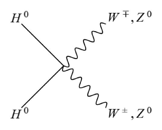
Figure 1: Annihilation into real W or Z boson pair, for $m_{H}>$ 90 GeV. These processes would produce a relic abundance of dark matter that is more than an order of magnitude too low to agree with the observed dark matter density.

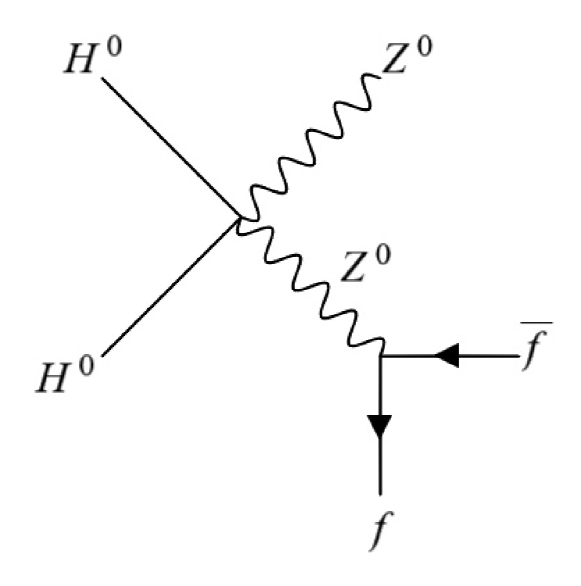
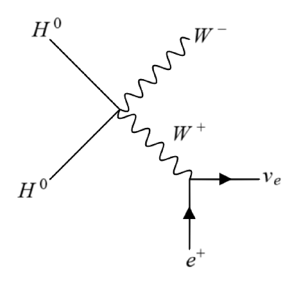
Figure 2: Left panel: Annihilation into one real and one virtual Z boson, for 90 GeV $>m_{H}>50$ GeV. There are 11 such processes for fermion-antifermion pairs $f\bar{f}$ (6 for leptons and 5 for the quarks with sufficiently low masses). Right panel: Example of annihilation into one real and one virtual W boson for 80 GeV $>m_{H}>43$ GeV. There are 18 such processes for fermion-antifermion pairs (6 for leptons and 12 for the quarks with sufficiently low masses). The total annihilation cross-section from these processes will be consistent with the observed relic abundance for $m_{H}\sim 72$ GeV.

For the processes of Fig. 1, we make the approximation that the $W$, $Z$, and $H$ masses are nearly equal ($\sim$ 80-100 GeV.). We find that the total annihilation cross-section is more than an order of magnitude too large for $m_{Z}>m_{H}>m_{W}$, and about a factor of 2 larger still for $m_{H}>m_{Z}$. (Without this approximation, the cross-sections would be even larger.) I.e., we obtain

$$\langle\sigma_{ann}v\rangle\gg\langle\sigma v\rangle_{S}\quad\ \mathrm{for}\quad m_{H}>m_{W}\approx 80\,\mathrm{GeV}$$ (65)

where $\langle\sigma v\rangle_{S}=2.2\times 10^{-26}\,\mathrm{cm}^{3}/\mathrm{s}$ is the benchmark value obtained by Steigman et al. [31] for a WIMP with mass above 10 GeV that is its own antiparticle, if the relic dark matter density is to agree with astronomical observations.

For the processes of Fig. 2, we make the approximation of neglecting the masses of the fermions (which are all small compared to $m_{Z}$, $m_{W}$, and $m_{H}$). There are 29 processes involving fermion-antifermion pairs. If $m_{H}$ is well below $m_{W}$, the total cross-section is more than an order of magnitude too small (compared again to $\langle\sigma v\rangle_{S})$.

As $m_{H}$ approaches $m_{W}$ from below, however, there is resonance-like behavior involving the $W$ propagator, and there is some value of $m_{H}$ (not precisely determined here because of the approximations described above) such that

$$\langle\sigma_{ann}v\rangle\sim\langle\sigma v\rangle_{S}\quad\mathrm{with}\quad m_{H}\sim 72\,\mathrm{GeV}\;.$$ (66)

This annihilation cross-section is consistent with the limits set by observation of gamma-ray emissions from dwarf spheroidal galaxies by Fermi-LAT [32, 33, 34], if the annihilation is treated generally rather than simplistically assumed to proceed through a single channel. For the present particle, there are 29 annihilation processes, represented by Fig. 2.

This cross-section and mass are also consistent with analyses of the gamma ray excess from the Galactic center observed by Fermi-LAT [35, 36, 37, 38, 39], and with analyses of the antiprotons observed by AMS [39, 40, 41, 42, 43], which independently have been interpreted as potential evidence of dark matter annihilation – although there are, of course, competing interpretations based on backgrounds and alternative statistical approaches. The inferred values of the particle mass and annihilation cross-section are in fact remarkably similar to those obtained here; see e.g. the abstracts of Refs. [37] and [42], and Fig. 12 of Ref. [43].

The predictions of the present theory within this context are very similar to those for the IDM if the masses of $A^{0}_{I}$ and $H^{\pm}_{I}$ are well separated from that of $H^{0}_{I}$. A very detailed analysis of the Fermi-LAT gamma-ray data, and its comparison with IDM predictions, has been given in [21]. For annihilations of a dark matter WIMP with a mass of $\sim 72$ GeV the basic qualitative conclusions are the same as above.

Collider detection of dark matter particles often focuses on creation through the $Z$, Higgs, or some hypothetical new mediator [44]. For the present particle there is no first-order coupling to the $Z$ and there are no exotic new mediators, so for this kind of process only the Higgs portal remains a possibility. CMS and ATLAS have independently placed upper limits on the branching ratio for invisible Higgs decays to particles with a total mass of $<125$ GeV [45, 46]. The present particle may have a small Higgs coupling, however, and the total mass of a pair should be $\sim$ 145 GeV. It appears that the present particle is also consistent with other collider-detection limits, and that the best possibility for observation in a collider experiment is the process depicted in Fig. 3.

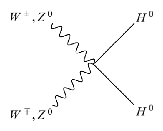
Figure 3: Collider creation through vector boson fusion.

The predicted signature for collider detection is then $\gtrsim$ 145 GeV of missing transverse energy resulting from vector boson fusion (VBF). In the present context this is a weak process, but the results of Refs. [23] and [24] (for the IDM), and [47] and [48] (for double Higgs production) suggest that observation of this process may be barely possible with a sustained run of the high-luminosity LHC, if an integrated luminosity of up to 3000 fb^-1 can be achieved. (Definitive studies may have to await a 100 TeV collider.) If there is a contribution from Higgs coupling, of course, the signal for creation of these particles will be stronger.

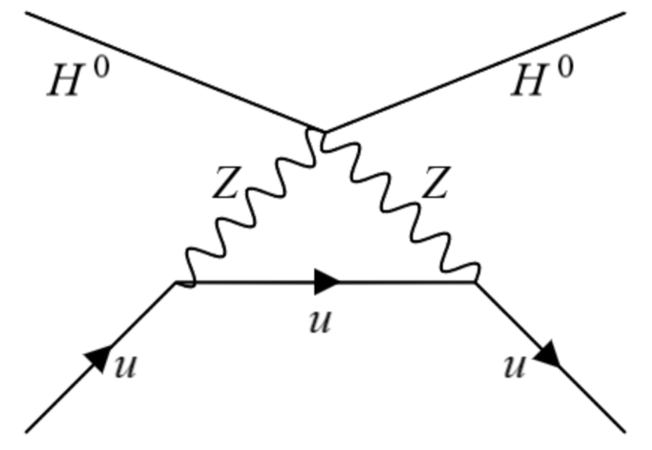
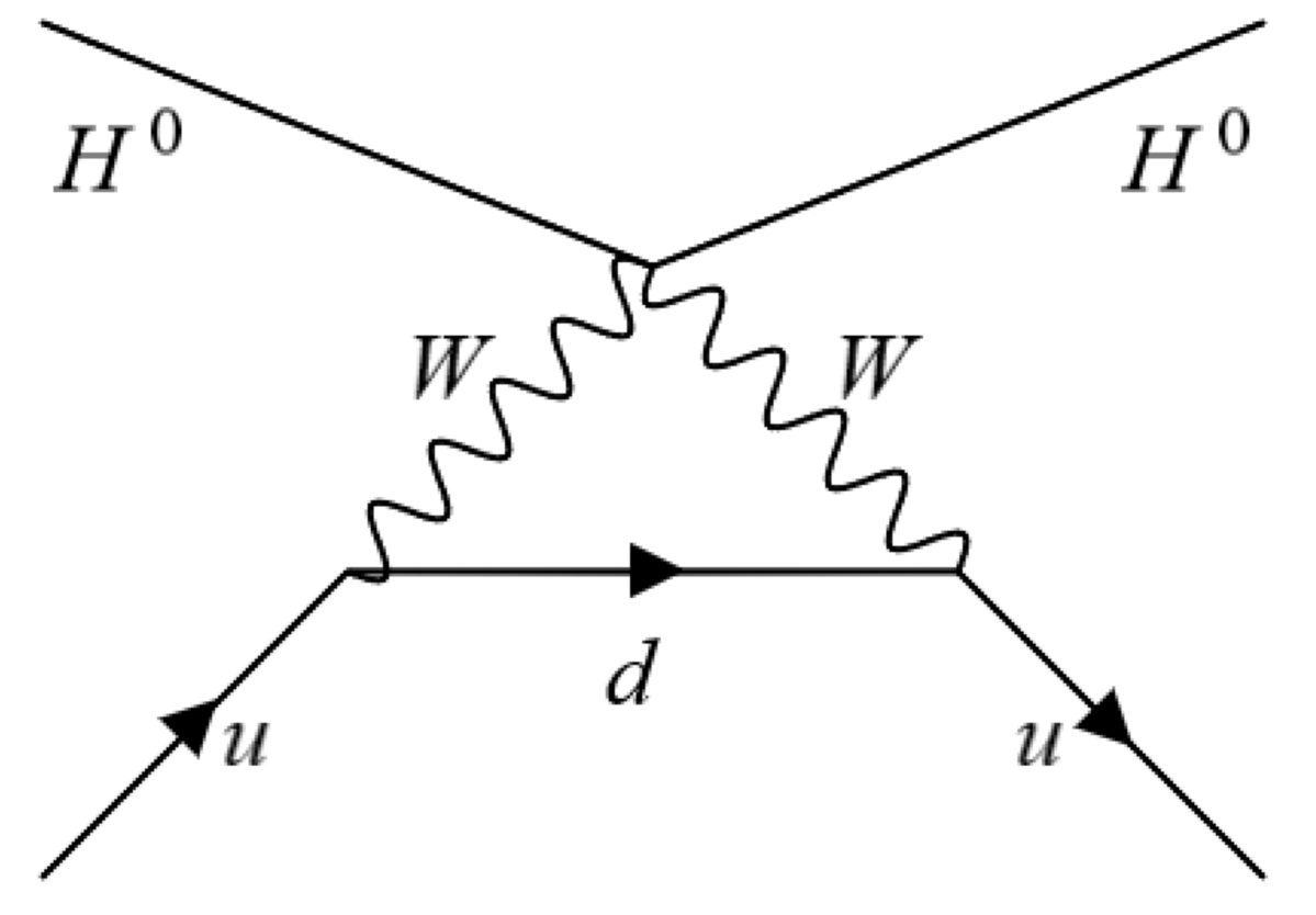
Figure 4: Scattering through loop processes, with a low but potentially accessible cross-section.

The best hope for direct detection appears to be the one-loop processes of Fig. 4, which are the same as for the IDM in Fig. 1 of [19]. The results in Figs. 2 and 3 of that paper suggest that this mechanism – scattering with an exchange of two Z or W bosons – has a cross-section not far below $10^{-11}$ pb for the present particle – perhaps barely within reach of sustained runs for the next generation of direct-detection experiments. Definitive studies would probably require even greater sensitivity, but with a cross-section still potentially attainable (and above the neutrino floor). Of course, there is again the possibility of some enhancement from Higgs exchange.

The present scenario is quite amenable to being tested by experiment and observation. For example, if the positron excess observed by AMS [49] (and other experiments) had demonstrated that the dominant dark matter particle has a mass of roughly 800 GeV or above, the much lower mass in the present scenario would have been disconfirmed. But the Planck observations have instead disconfirmed this interpretation [50]. On the other hand, the interpretation of a lower-mass dark-matter signal in the analyses cited above is quite consistent with the Planck data, and in addition is just as expected for thermal production.

We conclude with a broad comment: The behavior of spin 1/2 fermions and spin 1 gauge bosons has turned out to be far richer than originally envisioned (dating from the discovery of the electron in 1897 and the proposal of the photon in 1905), so one might anticipate further richness connected to the recent discovery of a spin 0 boson. In the present theory this boson represents the lowest-energy amplitude excitation in an extended Higgs sector.

- [1] G. Jungman, M. Kamionkowski, and K. Griest, “Supersymmetric Dark Matter”, Phys. Rept. 267, 195 (1996), arXiv:hep-ph/9506380.
- [2] Howard Baer, Vernon Barger, and Hasan Serce, “SUSY under siege from direct and indirect WIMP detection experiments”, Phys. Rev. D 94, 115019 (2016), arXiv:1609.06735 [hep-ph].
- [3] Howard Baer, Vernon Barger, Dibyashree Sengupta, and Xerxes Tata, “Is natural higgsino-only dark matter excluded?”, Eur. Phys. J. C 78, 838 (2018), arXiv:1803.11210 [hep-ph].
- [4] Leszek Roszkowski, Enrico Maria Sessolo, and Sebastian Trojanowski, “WIMP dark matter candidates and searches - current status and future prospects”, Rept. Prog. Phys. 81, 066201 (2018), arXiv:1707.06277 [hep-ph].
- [5] Howard Baer, Dibyashree Sengupta, Shadman Salam, Kuver Sinha, and Vernon Barger, “Midi-review: Status of weak scale supersymmetry after LHC Run 2 and ton-scale noble liquid WIMP searches”, arXiv:2002.03013 [hep-ph].
- [6] Xerxes Tata, “Natural Supersymmetry: Status and Prospects”, arXiv:2002.04429 [hep-ph].
- [7] R. E. Allen, “Predictions of a fundamental statistical picture”, arXiv:1101.0586 [hep-th].
- [8] Roland E. Allen and Aritra Saha, “Dark matter candidate with well-defined mass and couplings”, Mod. Phys. Lett. A 32, 1730022 (2017), arXiv:1706.00882 [hep-ph].
- [9] Roland E. Allen, “Saving supersymmetry and dark matter WIMPs – a new kind of dark matter candidate with well-defined mass and couplings”, Phys. Scr. 94, 014010 (2019), arXiv:1811.00670 [hep-ph].
- [10] Maxwell Throm, Reagan Thornberry, John Killough, Brian Sun, Gentill Abdulla, and Roland E. Allen. “Two natural scenarios for dark matter particles coexisting with supersymmetry”. Mod. Phys. Lett. A 34, 1930001 (2019), arXiv:1901.02781 [hep-ph].
- [11] Nilendra G. Deshpande and Ernest Ma, “Pattern of symmetry breaking with two Higgs doublets”, Phys. Rev. D 18, 2574 (1978).
- [12] Ernest Ma, “Verifiable radiative seesaw mechanism of neutrino mass and dark matter”, Phys. Rev. D 73, 077301 (2006), hep-ph/0601225.
- [13] Riccardo Barbieri, Lawrence J. Hall, and Vyacheslav S. Rychkov, “Improved naturalness with a heavy Higgs boson: An alternative road to CERN LHC physics”, Phys. Rev. D 74 015007 (2006), hep-ph/0603188.
- [14] Laura Lopez Honorez, Emmanuel Nezri, Josep F. Oliver, and Michel H. G. Tytgat, “The inert doublet model: an archetype for dark matter”, JCAP 02, 028 (2007), arXiv:hep-ph/0612275.
- [15] Erik Lundström, Michael Gustafsson, Joakim Edsjö, “Inert Doublet Model and LEP II Limits”, Phys. Rev. D 79, 035013 (2009), arXiv:0810.3924 [hep-ph].
- [16] Xinyu Miao, Shufang Su, and Brooks Thomas, “Trilepton Signals in the Inert Doublet Model”, Phys. Rev. D 82, 035009 (2010), arXiv:1005.0090 [hep-ph].
- [17] Laura Lopez Honorez and Carlos E. Yaguna, “The inert doublet model of dark matter revisited”, JHEP 09, 46 (2010), arXiv:1003.3125 [hep-ph].
- [18] Michael Gustafsson, Sara Rydbeck, Laura Lopez-Honorez, and Erik Lundström, “Status of the inert doublet model and the role of multileptons at the LHC”, Phys. Rev. D 86, 075019 (2012), arXiv:1206.6316 [hep-ph].
- [19] Michael Klasen, Carlos E. Yaguna, and José D. Ruiz-Álvarez, “ Electroweak corrections to the direct detection cross section of inert higgs dark matter”, Phys. Rev. D 87, 075025 (2013), arXiv:1302.1657 [hep-ph].
- [20] A. Goudelis, B. Herrmann, and O. Stål, “Dark matter in the inert doublet model after the discovery of a Higgs-like boson at the LHC”, JHEP 09, 106 (2013), arXiv:1303.3010 [hep-ph], and references therein.
- [21] Benedikt Eiteneuer, Andreas Goudelis, and Jan Heisig, “The inert doublet model in the light of Fermi-LAT gamma-ray data: a global fit analysis”, Eur. Phys. J. C 77, 624 (2017), arXiv:1705.01458 [hep-ph].
- [22] Alexander Belyaev, Giacomo Cacciapaglia, Igor P. Ivanov, Felipe Rojas-Abatte, and Marc Thomas, “Anatomy of the Inert Two Higgs Doublet Model in the light of the LHC and non-LHC Dark Matter Searches”, Phys. Rev. D 97, 035011 (2018), arXiv:1612.00511 [hep-ph], and references therein.
- [23] Bhaskar Dutta, Guillermo Palacio, Diego Restrepo, and José D. Ruiz-Álvarez, “Vector Boson Fusion in the Inert Doublet Model”, Phys. Rev. D 97, 055045 (2018), arXiv:1709.09796 [hep-ph].
- [24] Daniel Dercks and Tania Robens, “Constraining the Inert Doublet Model using Vector Boson Fusion”, Eur. Phys. J. C 79, 924 (2019), arXiv:1812.07913 [hep-ph].
- [25] Dorota Sokolowska, Jan Kalinowski, Jan Klamka, Pawel Sopicki, Aleksander Filip Żarnecki, Wojciech Kotlarski, Tania Robens, “Inert Doublet Model signatures at future colliders”, arXiv:1911.06254 [hep-ph].
- [26] A. Belyaev, T. R. Fernandez Perez Tomei, P. G. Mercadante, C. S. Moon, S. Moretti, S. F. Novaes, L. Panizzi, F. Rojas, M. Thomas, “Advancing LHC Probes of Dark Matter from the Inert 2-Higgs Doublet Model with the Mono-jet Signal”, Phys. Rev. D 99, 015011 (2019), arXiv:1809.00933 [hep-ph].
- [27] Shankha Banerjee, Fawzi Boudjema, Nabarun Chakrabarty, and Hao Sun, “Relic density of dark matter in the inert doublet model beyond leading order for the low mass region: 3. Annihilation in 3-body final state”, arXiv:2101.02167 [hep-ph].
- [28] D. Pekker and C. M. Varma, “Amplitude/Higgs Modes in Condensed Matter Physics”, Annu. Rev. Condens. Matter Phys. 6, 269 (2015), arXiv:1406.2968 [cond-mat.supr-con].
- [29] M. E. Peskin and D. V. Schroeder, An Introduction to Quantum Field Theory (Perseus, 1995).
- [30] T.-P. Cheng and L.-F. Li, Gauge theory of elementary particle physics (Oxford University Press, 1984).
- [31] G. Steigman, B. Dasgupta, and J. F. Beacom, “Precise relic WIMP abundance and its impact on searches for dark matter annihilation”, Phys. Rev. D 86 023506 (2012), arXiv:1204.3622 [hep-ph].
- [32] Rebecca K. Leane, Tracy R. Slatyer, John F. Beacom, and Kenny C. Y. Ng, “GeV-scale thermal WIMPs: Not even slightly ruled out”, Phys. Rev. D 98, 023016 (2018), arXiv:1805.10305 [hep-ph].
- [33] Shin’ichiro Ando, Alex Geringer-Sameth, Nagisa Hiroshima, Sebastian Hoof, Roberto Trotta, and Matthew G. Walker, “Structure Formation Models Weaken Limits on WIMP Dark Matter from Dwarf Spheroidal Galaxies”, Phys. Rev. D 102, 061302 (2020), arXiv:2002.11956 [astro-ph.CO].
- [34] Rebecca K. Leane, “Indirect Detection of Dark Matter in the Galaxy”, arXiv:2006.00513 [hep-ph].
- [35] Lisa Goodenough and Dan Hooper, “Possible Evidence For Dark Matter Annihilation In The Inner Milky Way From The Fermi Gamma Ray Space Telescope”, arXiv:0910.2998 [hep-ph].
- [36] Vincenzo Vitale and Aldo Morselli (for the Fermi/LAT Collaboration), “Indirect Search for Dark Matter from the center of the Milky Way with the Fermi-Large Area Telescope”, arXiv:0912.3828 [astro-ph.HE].
- [37] Christopher Karwin, Simona Murgia, Tim M. P. Tait, Troy A. Porter, and Philip Tanedo, “Dark matter interpretation of the Fermi-LAT observation toward the Galactic Center”, Phys. Rev. D 95, 103005 (2017), arXiv:1612.05687 [hep-ph], and references therein.
- [38] Rebecca K. Leane and Tracy R. Slatyer, “Revival of the Dark Matter Hypothesis for the Galactic Center Gamma-Ray Excess”, Phys. Rev. Lett. 123, 241101 (2019), arXiv:1904.08430 [astro-ph.HE], and references therein.
- [39] Alessandro Cuoco, Jan Heisig, Michael Korsmeier, and Michael Krämer, “Probing dark matter annihilation in the Galaxy with antiprotons and gamma rays”, JCAP 10, 053 (2017), arXiv:1704.08258 [astro-ph.HE].
- [40] Alessandro Cuoco, Michael Krämer, and Michael Korsmeier, “Novel dark matter constraints from antiprotons in the light of AMS-02”, Phys. Rev. Lett. 118, 191102 (2017), arXiv:1610.03071 [astro-ph.HE].
- [41] Ming-Yang Cui, Qiang Yuan, Yue-Lin Sming Tsai, and Yi-Zhong Fan, “Possible dark matter annihilation signal in the AMS-02 antiproton data”, Phys. Rev. Lett. 118, 191101 (2017), arXiv:1610.03840 [astro-ph.HE].
- [42] Ilias Cholis, Tim Linden, and Dan Hooper, “A Robust Excess in the Cosmic-Ray Antiproton Spectrum: Implications for Annihilating Dark Matter”, Phys. Rev. D 99, 103026 (2019), arXiv:1903.02549 [astro-ph.HE].
- [43] Alessandro Cuoco, Jan Heisig, Lukas Klamt, Michael Korsmeier, and Michael Krämer, “Scrutinizing the evidence for dark matter in cosmic-ray antiprotons”, Phys. Rev. D 99, 103014 (2019), arXiv:1903.01472 [astro-ph.HE].
- [44] Antonio Boveia and Caterina Doglioni, “Dark Matter Searches at Colliders”, Annu. Rev. Nucl. Part. Sci. 68, 429 (2018), arXiv:1810.12238 [hep-ex].
- [45] CMS Collaboration, “Search for invisible decays of a Higgs boson produced through vector boson fusion in proton-proton collisions at TeV”, Phys. Lett. B 793, 520 (2019), arXiv:1809.05937 [hep-ex].
- [46] M. Aaboud et al. (ATLAS Collaboration), “Combination of Searches for Invisible Higgs Boson Decays with the ATLAS Experiment” , Phys. Rev. Lett. 122, 231801 (2019), arXiv:1904.05105 [hep-ex].
- [47] Fady Bishara, Roberto Contino, and Juan Rojo, “Higgs pair production in vector-boson fusion at the LHC and beyond”, Eur. Phys. J. C 77, 481 (2017), arXiv:1611.03860 [hep-ph].
- [48] Frédéric A. Dreyer, Alexander Karlberg, Jean-Nicolas Lang, and Mathieu Pellen, “Precise predictions for double-Higgs production via vector-boson fusion”, Eur. Phys. J. C 80, 1037 (2020), arXiv:2005.13341 [hep-ph].
- [49] Dan Hooper, Ilias Cholis, Tim Linden, and Ke Fang, “HAWC Observations Strongly Favor Pulsar Interpretations of the Cosmic-Ray Positron Excess”, Phys. Rev. D 96, 103013 (2017), arXiv:1702.08436 [astro-ph.HE].
- [50] Planck Collaboration, “Planck 2018 results. VI. Cosmological parameters”, arXiv:1807.06209 [astro-ph.CO]. See Fig. 46 in particular.