Learning to Learn to be Right for the Right Reasons

Abstract

Improving model generalization on held-out data is one of the core objectives in commonsense reasoning. Recent work has shown that models trained on the dataset with superficial cues tend to perform well on the easy test set with superficial cues but perform poorly on the hard test set without superficial cues. Previous approaches have resorted to manual methods of encouraging models not to overfit to superficial cues. While some of the methods have improved performance on hard instances, they also lead to degraded performance on easy instances. Here, we propose to explicitly learn a model that does well on both the easy test set with superficial cues and hard test set without superficial cues. Using a meta-learning objective, we learn such a model that improves performance on both the easy test set and the hard test set. By evaluating our models on Choice of Plausible Alternatives (COPA) and Commonsense Explanation, we show that our proposed method leads to improved performance on both the easy test set and the hard test set upon which we observe up to 16.5 percentage points improvement over the baseline.

1 Introduction

Pre-trained language models such as BERT Devlin et al. (2019) and RoBERTa Liu et al. (2019) have enabled performance improvements on benchmarks of language understanding Wang et al. (2019a). However, improved performance is not only the result of increased ability to solve the benchmark tasks as intended, but also due to models’ increased ability to “cheat” by relying on superficial cues Gururangan et al. (2018); Sugawara et al. (2018); Niven and Kao (2019). That is, even though models may perform better in terms of benchmark scores, they often are right for the wrong reasons McCoy et al. (2019) and exhibit worse performance when prevented from exploiting superficial cues Gururangan et al. (2018); Sugawara et al. (2018); Niven and Kao (2019).

To analyze reliance on superficial cues and to evaluate methods that encourage models to be right for the right reasons, i.e., to solve tasks as intended, training instances can be divided into two categories Gururangan et al. (2018): easy training instances contain easily identifiable superficial cues, such as a word that strongly correlates with a class label so that the presence or absence of this word alone allows better-than-random prediction Niven and Kao (2019). In contrast, hard instances do not contain easily exploitable superficial cues and hence require non-trivial reasoning. Models that exploit superficial cues are characterized by a performance gap: they show high scores on easy instances, but much lower scores on hard ones.

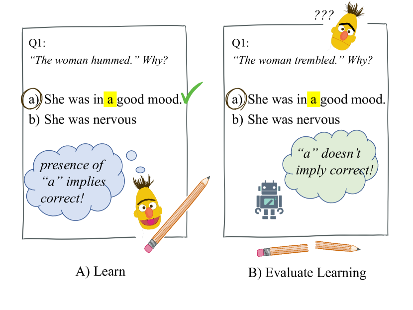
Figure 1: A modeling learning to be right for the right reason. A) shows a model wrongly learning that presence of “a” in the choice implies that the answer choice is correct. B) The models’ learning is tested after a few examples and uses this testing error to improve how it learns in the inner-loop. Hence, learning to learn to be right for the right reasons.

Previous work has aimed at countering superficial cues. A direct, if drastic, method is to completely remove easy instances from the training data via adversarial filtering Zellers et al. (2018), which leads to better performance on hard instances, but, as Gururangan et al. (2018) point out, filtering easy instances may harm performance by reducing the data diversity and size. Instead of completely removing easy instances, Schuster et al. (2019) propose a loss discounting scheme that assigns less weight to instances which likely contain superficial cues, while Belinkov et al. (2019) use adversarial training to penalize models for relying on superficial cues. A different approach, taken by Niven and Kao (2019) and Kavumba et al. (2019), is to augment datasets in a way that balances the distribution of superficial cues so that they become uninformative. Common to all these approaches is that reduced reliance on superficial cues is reflected in degraded performance on easy instances, while maintaining or increasing scores on hard instances.

Here we propose meta-learning as an alternative approach to reducing reliance on superficial cues, which, as we will show, improves performance on both easy and hard instances. Intuitively, we see reliance on superficial cues not as a defect of datasets, but as a failure to learn: If a model learns to rely on superficial cues, it will not generalize to instances without such cues, but if the model learns not to rely on such cues, this generalization will be possible. Conversely, a model that only learns how to solve hard instances may perform poorly on easy instances. Therefore, our meta-learned model learns how to generalize to both easy and hard instances. By evaluating our method on two English commonsense benchmarks, namely Choice of Plausible Alternatives (COPA) Roemmele et al. (2011) and Commonsense Explanation (Cs-Ex) Wang et al. (2019b), we show that meta-learning improves performance on both easy and hard instances and outperforms all baselines.

In summary, our contributions are:

1. We propose a meta-learning method that learns how to generalize to both easy and hard instances (§ 2),

2. We show that Commonsense Explanation Wang et al. (2019b) contain superficial cues that are easy to exploit by models (§ 3),

3. We empirically show that meta-learning a model to generalise to both easy and hard instances leads to better generalization not only on hard instances but also on easy instances (§ 4),

2 Learning to Generalize

2.1 Background

Meta-learning has been successfully applied to problems such as few-shot learning Vinyals et al. (2016); Finn et al. (2017) and continual learning Javed and White (2019); Beaulieu et al. (2020).

A meta-learning or learning to learn procedure consists of two phases. The first phase, also called meta-training, consists of learning in two nested loops. Learning starts in the inner loop where the models’ parameters are updated using the meta-training training set. At the end of the inner loop updates, the models’ inner loop learning of the task is meta-train tested in outer loop where a separate meta-training testing set is used. This is called meta-training testing. Unlike a non-meta-training process, the meta-training testing error is also used to update the model parameters, i.e., the meta-training testing error is used to improve the inner loop. Thus, learning is performed in both the inner and the outer loop, hence, learning-to-learn.

The second phase, also called meta-testing, consists only of a single loop. Model parameters are finetuned on a meta-testing training set and finally evaluated, only once, on the held out meta-testing testing set. Note that the meta-testing testing set is different from the meta-training testing set.

One of the most popular meta-learning algorithms is Model-Agnostic Meta-Learning (MAML) algorithm Finn et al. (2017). MAML is a few-shot optimization-based meta-learning algorithm whose goal is to learn initial model parameters $\theta$ for multiple related tasks such that a few gradient updates lead to optimal performance on target tasks. We choose MAML for our experiments because it is model agnostic and, hence, widely applicable.

2.2 Meta-Learning to Generalize

Our goal is to learn a model $f_{\theta}$, with parameters $\theta$, that generalizes well on both easy instances, with superficial cues, and hard instances, without superficial cues. Specifically, given a large single-task training set $D^{tr}$, we want to be able to train a model that generalizes well to both the easy test set $D^{test\_easy}$ and the hard test set $D^{test\_hard}$. To learn such a model, we require a meta-training testing set, $D^{tr_{t}est}$, which contains both easy and hard instances. Such a meta-training testing set will ensure that we evaluate the model generalization to both easy and hard instances. Optimizing only for better performance on hard instances can lead to poor generalization to easy instances Gururangan et al. (2018).

We cannot naively apply the meta-learning method designed for learning multiple few-shot tasks to a large dataset. A large dataset presents three main challenges. First, a naive meta-learning method would require using the entire training set during each inner loop update. This would make training very slow and computationally expensive. To address this problem, we use small randomly sampled batches in each inner loop. This is similar to treating each mini-batch as a single MAML task.

Second, a naive meta-learning method would require using the entire meta-training testing set for each outer loop update. This, too, would make learning very slow when the meta-training testing set is large. We address this challenge by evaluating the inner loop learning using only a small batch that is randomly drawn from the meta-training testing set.

Third, a naive meta-learning method would require storing the entire inner loop computation graph to facilitate second-order gradients’ computation. However, for large datasets and large models, such as recent pre-trained language models used in this paper, this is computationally too expensive and impractical on current hardware. To address this problem, we use first-order MAML Finn et al. (2017) that uses only the last inner-update.

We call this method of using random meta-training training batches and meta-training testing batches for meta-updates as Stochastic-Update Meta-Learning (SUML, Algorithm 1). The hyperparameter k is the number of inner loop updates performed for each outer loop update (i.e., i in Algorithm 1 ranges from 1 to k). Setting the value of k to 1 would make training unstable, much like using a batch size of 1 in standard (non-meta) training. On the other hand, a large value of k would make training slow.

Effectively, the model is meta-trained to use any batch in the training set to perform well on both the easy and the hard instances.

Algorithm 1 Stochastic-Update Meta-Learning

0:  $D^{tr}$: Training set

0:  $D^{tr\_test}$: Balanced meta-training test set

0:  $\alpha$: inner-loop step size

0:  $\beta$: outer-loop step size

1:  $\theta$: LM pretrained parameters

2:  while not done do

3:     Sample batch $D_{j}^{tr\_test}$ from $D^{tr\_test}$

4:     for $i=1,2,3,...,k$ do

5:        Sample batch $D_{i}^{tr}$ from $D^{tr}$

6:        Adapt parameters with gradient descent: $\theta_{i}=\theta_{i-1}-\alpha\nabla_{\theta}L(f_{\theta_{i-1}},D_{i}^{tr})$

7:     end for

8:     Update $\theta\leftarrow\theta-\beta\nabla_{\theta}L(f_{\theta_{k}},D_{j}^{tr\_test})$

9:  end while

3 Superficial Cues in COPA and Commonsense Explanation

3.1 Datasets

Here, we briefly describe the English commonsense datasets that we use in this paper.

Model Ensemble Data Easy Hard Overall SuperGlue Leaderboard Score:    RoBERTa-large + ALBERT-xxLarge yes COPA - - 90.8    RoBERTa-large yes COPA - - 90.6 RoBERTa-large no COPA 90.5 83.9 86.4 RoBERTa-large-adversarial no COPA 70.0 56.5 61.6 RoBERTa-large + Balanced data no B-COPA 90.0 88.1 88.8 RoBERTa-large-meta-learned (ours) no COPA 92.6 89.7 90.8 RoBERTa-base no COPA 80.0 71.3 74.6 RoBERTa-base-adversarial no COPA 76.3 57.0 64.4 RoBERTa-base no B-COPA 78.4 78.1 78.2 RoBERTa-base-meta-learned (ours) no COPA 87.9 78.4 82.0 RoBERTa-large no Cs-Ex 98.0 79.1 93.8 RoBERTa-large-adversarial no Cs-Ex 94.0 59.0 86.2 RoBERTa-large-meta-learned (ours) no Cs-Ex 98.9 87.1 96.2 RoBERTa-base no Cs-Ex 95.0 62.1 87.7 RoBERTa-base-adversarial no Cs-Ex 93.8 54.8 85.2 RoBERTa-base-meta-learned (ours) no Cs-Ex 97.6 78.6 93.4

Table 1: Accuracy on Easy and Hard instances. We report accuracy for models trained on COPA, Balanced COPA (B-COPA) and Commonsense Explanation (Cs-Ex). We also report SuperGlue Wang et al. (2019a) leaderboard scores for single task fine-tuning for reference.

Balanced COPA: The Balanced Choice of Plausible Alternatives (Kavumba et al., 2019, Balanced COPA) counters superficial cues in the answer choices of the Choice of Plausible Alternatives (Roemmele et al., 2011, COPA) by balancing token distribution between correct and wrong answer choices. Balanced COPA creates mirrored instances for each of the original instance in the training set. Concretely, for each original COPA instance shown below:

Premise: The stain came out of the shirt. What was the CAUSE of this?

a) I bleached the shirt. (Correct)

b) I patched the shirt.

Balanced COPA creates another instance that shares the same alternatives but a different manually authored premise. The wrong answer choice the original question is made correct by the new premise (refer to App. B for more examples).

Premise: The shirt did not have a hole anymore. What was the CAUSE of this?

a) I bleached the shirt.

b) I patched the shirt. (Correct)

This counters superficial cues by balancing the token distribution in the answer choices.

Commonsense Explanation: Commonsense Explanation (Cs-Ex) Wang et al. (2019b) is a multiple-choice benchmark that consists of three subtasks. Here we focus on a commonsense explanation task. Given a false statement such as He drinks apple., Cs-Ex requires a model to pick the reason why a false statement does not make sense, in this case either: a) Apple juice are very tasty and milk too; or b) Apple can not be drunk (correct); or c) Apple cannot eat a human.

3.2 Superficial cues in Cs-Ex

While COPA has already been shown to contain superficial cues by Kavumba et al. (2019), Cs-Ex has not been analyzed yet. Here, we present an analysis of superficial cues in Cs-Ex.

We fine-tuned RoBERTa-base and RoBERTa-large with contextless inputs (answers only). This reveals the models’ ability to rely on shortcuts such as different token distributions in correct and wrong answers Gururangan et al. (2018); McCoy et al. (2019).

In this setting, we expect the models’ accuracy to be nearly random if the answer choices have no superficial cues. But, we find that RoBERTa performs better than random accuracy of 33.3%. The above-random performance of RoBERTa-base (82.1%) and RoBERTa-large (85.4%) indicates that the answers of Cs-Ex contain superficial cues.

To identify the actual superficial cues a model can exploit, we collect words/unigrams that are predictive of the correct answer choice using the productivity measure introduced by Niven and Kao (2019, see definition in App. A). Intuitively, the productivity of a token expresses how precise a model would be if it based its prediction only on the presence of this token in a candidate answer. We found that the word not was highly predictive of the correct answer, followed by the word to (See details in App. A).

3.3 Easy and Hard Instances

Following previous work Gururangan et al. (2018); Kavumba et al. (2019), we split the test set of Cs-Ex into an easy and hard subset. The easy subset consists of all instances (1,572) that RoBERTa-base solved correctly across three different runs in the contextless input (answer only) setting. All the remaining instances, 449, are considered hard instances. For COPA, we use the easy and hard subset splits from Kavumba et al. (2019), which consists of 190 easy and 310 hard instances.

4 Experiments

4.1 Training Details

In our experiments, we used a recent state-of-the-art large pre-trained language model, namely RoBERTa Liu et al. (2019)—an optimized variant of BERT Devlin et al. (2019). Specifically, we used RoBERTa-base and RoBERTa-large with 110M and 355M parameters, respectively, from the publicly available Huggingface source code Wolf et al. (2019).  We ran all our experiments on a single NVIDIA Tesla V100 GPU with 16GB memory.

We used an Adam optimizer Kingma and Ba (2015) with a warm-up proportion of 0.06 and a weight decay of 0.01. We randomly split the training data into training data and validation data with a ratio of 9:1. We trained the models for a maximum of 10 epochs with early stopping based on the validation loss (full training details in App. C).

4.2 COPA

To evaluate the effectiveness of meta-learning a model to be robust against superficial cues, we compare our model that is meta-trained on 450 original COPA instances and 100 balanced meta-training testing examples with three different baselines. Specifically, we compare to:
1. A model trained on 500 original COPA instances.
2. An adversarial trained model to avoid the answer only superficial cues on 500 original COPA instances.
3. A model trained on 1000 Balanced COPA instances, manually created to counter superficial cues. In comparison, our meta-trained model uses only a small fraction of balanced instances. Effectively, our method replaces the need to have a large balanced training set with a small, 100 instances, in this case, meta-training test set.

The results show that the models trained on the original COPA perform considerably better on the easy subset (90.5%) than on the hard subset (83.9%) (Table 1). The models trained on balanced COPA improves performance on the hard subset (88.1%) but slightly degrades performance on the easy subset (90.0%). This indicates that training on Balanced COPA improves generalization on the hard instances. As expected, the performance of the adversarial trained model is lower than the vanilla baselines. This finding is similar to the result found in natural language inference Belinkov et al. (2019). Comparing our meta-trained models to the baselines, we see that meta-training improves performance on both the easy subset and hard subset. Our meta-trained models even outperform the models trained on nearly twice the training data and an ensemble of RoBERT-large. It even matches an ensemble of RoBERTa-large and ALBERT-xxlarge Lan et al. (2019). 

4.3 Commonsense Explanation

This experiment aims to investigate an automatic method of creating a meta-training testing set. Here we assume that there is no budget for manually creating a small meta-training testing set as in Balanced COPA. We created a meta-training testing set by randomly sampling 288 hard instances. Gururangan et al. (2018) pointed out that optimizing only for hard instance might lead to poor performance on easy instance. This observation motivates us to include both easy and hard instances in the meta-training testing set, with the expectation that this will ensure that performance on easy instances does not degrade. We augmented the hard instances with an equal number of randomly sampled easy instances, resulting into the final meta-training testing set with 576 instances.

The results show that the meta-trained models perform better than the baselines on both easy and hard instances (Table 1). For RoBERTa-large we see 0.9 percentage point improvement on easy instances and eight percentage points improvement on the hard instances. We see the largest gains on the RoBERTa-base with 2.6 and 16.5 percentage points on easy and hard instances, respectively. The results indicate that in the absence of a manually authored meta-training testing set without superficial cues, we can use a combination of easy and hard instances.

5 Conclusion

We propose to directly learn a model that performs well on both instances with superficial cues and instances without superficial cues via a meta-learning objective. We carefully evaluate our models, which are meta-learned to improve generalization, on two important commonsense benchmarks, finding that our proposed method considerably improves performance across all test sets.

Appendix

Appendix A Identifying Superficial Cues

We identify tokens predictive of the correct answer using productivity, as defined by Niven and Kao (2019). Let $\mathbb{T}_{j}^{(i)}$ be the set of tokens in the alternatives for data point ${i}$ with label ${j}$. The applicability ${\alpha}_{k}$ of a token $k$ counts how often this token occurs in an alternative with one label, but not the other:

$$\alpha_{k}=\sum_{i=1}^{n}\mathbbm{1}\left[\exists j,k\in\mathbb{T}_{j}^{(i)}\wedge k\notin\mathbb{T}_{\neg j}^{(i)}\right]$$

The productivity $\pi_{k}$ of a token is the proportion of applicable instances for which it predicts the correct answer:

$$\pi_{k}=\frac{\sum_{i=1}^{n}\mathbbm{1}\left[\exists j,k\in\mathbb{T}_{j}^{(i)}\wedge k\notin\mathbb{T}_{\neg j}^{(i)}\wedge y_{i}=j\right]}{\alpha_{k}}$$

The most productive tokens in Cs-Exshown in Table 2.

Appendix B Dataset

We use English datasets, namely COPA  Roemmele et al. (2011), Balanced COPA  Kavumba et al. (2019), and Commonsense Explanation  Wang et al. (2019b) for all our experiments.

B.1 Balanced COPA

The Balanced Choice of Plausible Alternatives (Kavumba et al., 2019, Balanced COPA) counters superficial cues in the answer choices by extending the training set of Choice of Plausible Alternatives (Roemmele et al., 2011, COPA) with twin questions for each of the original COPA instances. Examples of twin questions are shown below:

Example 1:
Original instance

Premise: My body cast a shadow over the grass. What was the CAUSE of this?

a) The sun was rising. (Correct)

b) The grass was cut.

Mirrored instance:

Premise: The garden looked well-groomed.. What was the CAUSE of this?

a) The sun was rising.

b) The grass was cut. (Correct)

Example 2:
Original instance

Premise: The woman tolerated her friend’s difficult behavior. What was the CAUSE of this?

a) The woman knew her friend was going through a hard time. (Correct)

b) The woman felt that her friend took advantage of her kindness.

Mirrored instance:

Premise: The woman did not tolerate her friend’s difficult behavior anymore.. What was the CAUSE of this?

a) The woman knew her friend was going through a hard time.

b) The woman felt that her friend took advantage of her kindness. (Correct)

B.2 Commonsense Explanation

Commonsense Explanation (Cs-Ex) Wang et al. (2019b) is a multiple-choice benchmark that consists of three subtasks. Here we focus on a commonsense explanation task. Given a false statement, Cs-Ex requires a model to pick the reason why a false statement does not make sense. For example:

FalseStatement: He drinks apple.

a) Apple juice are very tasty and milk too

b) Apple can not be drunk (correct)

c) Apple cannot eat a human

Appendix C Training Details

In our experiments, we use a state-of-the-art recent pre-trained language model, namely RoBERTa Liu et al. (2019), an optimized variant of BERT Devlin et al. (2019). We use RoBERTa-base and RoBERTa-large with 110M and 355M parameters respectively from the publicly available Huggingface source code Wolf et al. (2019). . We run all our experiments on a single NVIDIA Tesla V100 GPU with 16GB memory.

We use Adam Kingma and Ba (2015) with a warm-up proportion of 0.06 and a weight decay of 0.01. We randomly split the training data into training data and validation data with a ratio of 9:1. We train the models for a maximum of 10 epochs with early stopping based on the validation loss.

C.1 COPA Baselines

Dataset Word Train Dev Prod. Cov. Prod. Cov. Cs-Ex not 72 47 59 40 to 35 37 33 43

Table 2: Productivity (Prod.) and Coverage (Cov.) of the top 2 most productive tokens in each dataset. We have highlighted the most productive results. In Commonsense-Explanation, if one always picks an option with ‘not’ then one can achieve 59% with a coverage of 40% data points on the dev set.

We use grid search for hyperparameter from learning rates {1e-5, 8e-6, 6e-6, 4e-6, 2e-6, 1e-6}, batch sizes {4, 8, 16, 32, 64}, gradient accumulation {1, 2, 4, 8}, Adam $\beta_{2}$ {0.98, 0.99}, and with gradient norm clipping of 1 and no gradient norm clipping. We pick the best performing hyperparameters on the validation set.

C.2 Commonsense Explanation (Cs-Ex) Baselines

We test learning rates 1e-5, 8e-6, 6e-6, 4e-6, 2e-6 and 1e-6, Adam $\beta_{2}$ 0.99, and with gradient norm clipping of 1. For RoBERTa-base, we use batch sizes of 64 with gradient accumulation 1, and for RoBERTa-large, we use a batch size of 32 with gradient accumulation 2. We pick the best performing hyperparameters on the validation set.

C.3 Adversarial Trained Baseline

We follow the setup defined by Belinkov et al. (2019). Specifically we optimize the objective function:

$\begin{aligned} L&=L_{\mathrm{scorer}}+\lambda_{\mathrm{Loss}}L_{\mathrm{Adv}}\\ L_{\mathrm{Adv}}&=L\left(c_{\mathrm{choice}}\left(\lambda_{\mathrm{Enc}}\operatorname{GRL}_{\lambda}\left(g_{C}(C)\right),y\right)\right)\end{aligned}$ Where $L_{\mathrm{scorer}}$ is the loss of the multiple-choice scorer (or head), $GRL_{\lambda}$ is the gradient reversal layer Ganin and Lempitsky (2015), $\lambda_{\mathrm{Loss}}$ is the importance of the adversarial loss ($L_{\mathrm{Adv}}$), $\lambda_{\mathrm{Enc}}$ is the scaling factor that multiplies the gradients after reversing them, $c_{\mathrm{choice}}$ maps the answer choice representation $C$ to an output y. The goal is to obtain a representation $g_{C}(C)$ so that it is maximally informative for multiple-choice answering while simultaneously minimizes the ability of $c_{\mathrm{choice}}$ to accurately predict the correct choice (refer to Belinkov et al. (2019) for further details). We use grid search to tune hyperparameters $\lambda_{\mathrm{Enc}}$ {0.1, 0.2, 0.3, 0.4, 0.5, 0.6, 0.7, 0.8, 0.9, 1 } and $\lambda_{\mathrm{Loss}}$ {0.1, 0.2, 0.3, 0.4, 0.5, 0.6, 0.7, 0.8, 0.9, 1 } and report the best performing results on the development set.

C.4 Meta-Training

In the inner-loop, we pick the maximum batch size that fits in GPU memory. For all the experiments, we use vanilla Stochastic Gradient Descent for the inner-loop with learning rate $\alpha$ 0.01 (it worked well in the first run therefore we do not modify it for the rest of the experiments), and Adam for the outer-loop with learning rate $\beta$ 1e-5 (based on the best learning rate for the RoBERTa baseline).

References

- Beaulieu et al. (2020) Shawn Beaulieu, Lapo Frati, Thomas Miconi, Joel Lehman, Kenneth O. Stanley, Jeff Clune, and Nick Cheney. 2020. Learning to continually learn.
- Belinkov et al. (2019) Yonatan Belinkov, Adam Poliak, Stuart Shieber, Benjamin Van Durme, and Alexander Rush. 2019. On adversarial removal of hypothesis-only bias in natural language inference. In Proceedings of the Eighth Joint Conference on Lexical and Computational Semantics (*SEM 2019), pages 256–262, Minneapolis, Minnesota. Association for Computational Linguistics.
- Devlin et al. (2019) Jacob Devlin, Ming-Wei Chang, Kenton Lee, and Kristina Toutanova. 2019. BERT: Pre-training of deep bidirectional transformers for language understanding. In Proceedings of the 2019 Conference of the North American Chapter of the Association for Computational Linguistics: Human Language Technologies, Volume 1 (Long and Short Papers), pages 4171–4186, Minneapolis, Minnesota. Association for Computational Linguistics.
- Finn et al. (2017) Chelsea Finn, Pieter Abbeel, and Sergey Levine. 2017. Model-agnostic meta-learning for fast adaptation of deep networks. volume 70 of Proceedings of Machine Learning Research, pages 1126–1135, International Convention Centre, Sydney, Australia. PMLR.
- Ganin and Lempitsky (2015) Yaroslav Ganin and Victor Lempitsky. 2015. Unsupervised domain adaptation by backpropagation. In Proceedings of the 32nd International Conference on Machine Learning, volume 37 of Proceedings of Machine Learning Research, pages 1180–1189, Lille, France. PMLR.
- Gururangan et al. (2018) Suchin Gururangan, Swabha Swayamdipta, Omer Levy, Roy Schwartz, Samuel Bowman, and Noah A. Smith. 2018. Annotation artifacts in natural language inference data. In Proceedings of the 2018 Conference of the North American Chapter of the Association for Computational Linguistics: Human Language Technologies, Volume 2 (Short Papers), pages 107–112, New Orleans, Louisiana. Association for Computational Linguistics.
- Javed and White (2019) Khurram Javed and Martha White. 2019. Meta-learning representations for continual learning. In Advances in Neural Information Processing Systems, volume 32, pages 1820–1830. Curran Associates, Inc.
- Kavumba et al. (2019) Pride Kavumba, Naoya Inoue, Benjamin Heinzerling, Keshav Singh, Paul Reisert, and Kentaro Inui. 2019. When choosing plausible alternatives, clever hans can be clever. In Proceedings of the First Workshop on Commonsense Inference in Natural Language Processing, pages 33–42, Hong Kong, China. Association for Computational Linguistics.
- Kingma and Ba (2015) Diederik P. Kingma and Jimmy Ba. 2015. Adam: A method for stochastic optimization. In 3rd International Conference on Learning Representations, ICLR 2015, San Diego, CA, USA, May 7-9, 2015, Conference Track Proceedings.
- Lan et al. (2019) Zhenzhong Lan, Mingda Chen, Sebastian Goodman, Kevin Gimpel, Piyush Sharma, and Radu Soricut. 2019. Albert: A lite bert for self-supervised learning of language representations.
- Liu et al. (2019) Yinhan Liu, Myle Ott, Naman Goyal, Jingfei Du, Mandar Joshi, Danqi Chen, Omer Levy, Mike Lewis, Luke Zettlemoyer, and Veselin Stoyanov. 2019. Roberta: A robustly optimized BERT pretraining approach. CoRR, abs/1907.11692.
- McCoy et al. (2019) Tom McCoy, Ellie Pavlick, and Tal Linzen. 2019. Right for the wrong reasons: Diagnosing syntactic heuristics in natural language inference. In Proceedings of the 57th Annual Meeting of the Association for Computational Linguistics, pages 3428–3448, Florence, Italy. Association for Computational Linguistics.
- Niven and Kao (2019) Timothy Niven and Hung-Yu Kao. 2019. Probing neural network comprehension of natural language arguments. In Proceedings of the 57th Annual Meeting of the Association for Computational Linguistics, pages 4658–4664, Florence, Italy. Association for Computational Linguistics.
- Roemmele et al. (2011) Melissa Roemmele, Cosmin Adrian Bejan, and Andrew S Gordon. 2011. Choice of plausible alternatives: An evaluation of commonsense causal reasoning. In AAAI Spring Symposium on Logical Formalizations of Commonsense Reasoning, Stanford University.
- Schuster et al. (2019) Tal Schuster, Darsh Shah, Yun Jie Serene Yeo, Daniel Roberto Filizzola Ortiz, Enrico Santus, and Regina Barzilay. 2019. Towards debiasing fact verification models. In Proceedings of the 2019 Conference on Empirical Methods in Natural Language Processing and the 9th International Joint Conference on Natural Language Processing (EMNLP-IJCNLP), pages 3410–3416, Hong Kong, China. Association for Computational Linguistics.
- Sugawara et al. (2018) Saku Sugawara, Kentaro Inui, Satoshi Sekine, and Akiko Aizawa. 2018. What makes reading comprehension questions easier? In Proceedings of the 2018 Conference on Empirical Methods in Natural Language Processing, pages 4208–4219, Brussels, Belgium. Association for Computational Linguistics.
- Vinyals et al. (2016) Oriol Vinyals, Charles Blundell, Timothy Lillicrap, koray kavukcuoglu, and Daan Wierstra. 2016. Matching networks for one shot learning. In Advances in Neural Information Processing Systems, volume 29, pages 3630–3638. Curran Associates, Inc.
- Wang et al. (2019a) Alex Wang, Yada Pruksachatkun, Nikita Nangia, Amanpreet Singh, Julian Michael, Felix Hill, Omer Levy, and Samuel R. Bowman. 2019a. SuperGLUE: A stickier benchmark for general-purpose language understanding systems. arXiv preprint 1905.00537.
- Wang et al. (2019b) Cunxiang Wang, Shuailong Liang, Yue Zhang, Xiaonan Li, and Tian Gao. 2019b. Does it make sense? and why? a pilot study for sense making and explanation. In Proceedings of the 57th Annual Meeting of the Association for Computational Linguistics, pages 4020–4026, Florence, Italy. Association for Computational Linguistics.
- Wolf et al. (2019) Thomas Wolf, Lysandre Debut, Victor Sanh, Julien Chaumond, Clement Delangue, Anthony Moi, Pierric Cistac, Tim Rault, R’emi Louf, Morgan Funtowicz, and Jamie Brew. 2019. Huggingface’s transformers: State-of-the-art natural language processing. ArXiv, abs/1910.03771.
- Zellers et al. (2018) Rowan Zellers, Yonatan Bisk, Roy Schwartz, and Yejin Choi. 2018. SWAG: A large-scale adversarial dataset for grounded commonsense inference. In Proceedings of the 2018 Conference on Empirical Methods in Natural Language Processing, pages 93–104, Brussels, Belgium. Association for Computational Linguistics.