Soliton interferometry with very narrow barriers obtained from spatially dependent dressed states

Abstract

Bright solitons in atomic Bose–Einstein condensates are strong candidates for high precision matter-wave interferometry, as their inherent stability against dispersion supports long interrogation times. An analog to a beam splitter is then a narrow potential barrier. A very narrow barrier is desirable for interferometric purposes, but in a typical realisation using a blue-detuned optical dipole potential, the width is limited by the laser wavelength. We investigate a soliton interferometry scheme using the geometric scalar potential experienced by atoms in a spatially dependent dark state to overcome this limit. We propose a possible implementation and numerically probe the effects of deviations from the ideal configuration.

Bright solitons are well-known within one-dimensional mean-field models of elongated attractively-interacting Bose–Einstein condensates (BECs). They have been realized Strecker et al. (2002); Khaykovich et al. (2002); Cornish et al. (2006); Lepoutre et al. (2016); Mežnaršič et al. (2019); Di Carli et al. (2019) in BECs of several species sol , and have much-discussed potential for atomic interferometry Veretenov et al. (2007); Abdullaev and Brazhnyi (2012); Martin and Ruostekoski (2012); Helm et al. (2012); Polo and Ahufinger (2013); Cuevas et al. (2013); Helm et al. (2015); Sakaguchi and Malomed (2016); McDonald et al. (2014); Haine (2018), owing to long interrogation times enabled by their self-support against dispersion, and to the phase-sensitivity of soliton collisions Nguyen et al. (2014). Colliding solitons with potential barriers is a convenient method to create two phase-coherent solitons, and to recombine two solitons into a phase-dependent output, forming the essential elements of an interferometer. In the limit of high collisional velocity, and a barrier narrow relative to the soliton width, a single incident soliton splits into two solitons with well-defined relative phase Martin and Ruostekoski (2012); Helm et al. (2012); Polo and Ahufinger (2013). Under the same conditions two solitons colliding “head-on” at a barrier recombine with output populations dependent on the incident solitons’ relative phase Martin and Ruostekoski (2012); Helm et al. (2012). These splitting and recombination processes have recently been investigated experimentally Wales et al. (2020); in a typical setup, focused blue-detuned laser beams realize barriers on the micron scale, comparable to a typical soliton width Marchant et al. (2013); Wales et al. (2020). How to generate narrower potential barriers required for optimal interferometry remains an important question. A known method to produce subwavelength features is via rapid change over a small region of the amplitude of one of two near-resonant laser fields in an atomic $\Lambda$ configuration, which can be understood in terms of effective potentials experienced by spatially dependent dressed states Łącki et al. (2016); Jendrzejewski et al. (2016); Ge and Zubairy (2020); Subhankar et al. (2019); Bienias et al. (2020); Tsui et al. (2020); Kapale and Agarwal (2010); Dum and Olshanii (1996); Goldman et al. (2014). We propose a technique exploiting these properties to create a single narrow barrier for soliton interferometry within a quasi-one-dimensional (quasi-1D) BEC. We subject our proposal to detailed numerical analysis of both the full $\Lambda$-system and an effective single-state model, showing it to provide potentially excellent interferometric performance within an experimentally reasonable regime.

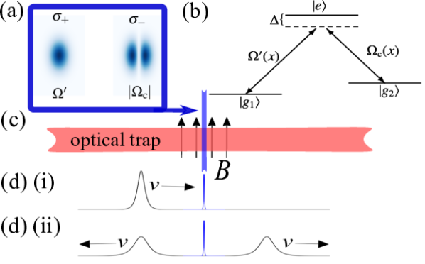
Figure 1: Proposed coherent soliton splitting scheme. (a) Profiles of differently polarized $\Omega^{\prime}$ and $\Omega_{\mathrm{c}}$ barrier-forming beams in the $x,z$ plane at $y=0$. (b) Atomic level configuration; we typically consider $\Delta=0$. (c) Schematic of an optical waveguide used to contain the solitons; a magnetic bias field $\bm{B}$ parallel to the $\Omega^{\prime}$ and $\Omega_{\mathrm{c}}$ beams provides a quantization axis. (d)(i) An initial velocity $v$ soliton propagating in the $+x$ direction (d)(ii) splits into two equal-size counterpropagating solitons.

We require three internal (hyperfine) atomic states, labelled $\ket{g_{1}}$, $\ket{g_{2}}$, and $\ket{e}$ in order of increasing energy, coupled in a $\Lambda$ configuration. We consider on-resonant couplings and neglect spontaneous decay from $\ket{e}$. The appropriate quasi-1D vector Gross–Pitaevskii equation (GPE) for a BEC of $N$ mass $m$ atoms, transversely confined by a tight harmonic trapping potential of angular frequency $\omega_{r}$, is

$$i\hbar\frac{\partial\psi_{j}}{\partial t}=-\frac{\hbar^{2}}{2m}\frac{\partial^{2}\psi_{j}}{\partial x^{2}}+\sum_{k}\left(g^{1\mathrm{D}}_{jk}|\psi_{k}|^{2}\psi_{j}+\frac{\hbar\Omega_{jk}}{2}\psi_{k}\right),$$ (1)

where $j,k\in\{g_{1},g_{2},e\}$, $g^{1\mathrm{D}}_{jk}=2\hbar\omega_{r}a_{jk}$, the probe beam Rabi frequency $\Omega_{1e}=\Omega_{e1}=\Omega^{\prime}(x)$, the control beam Rabi frequency $\Omega_{2e}=\Omega_{e2}=\Omega_{\mathrm{c}}(x)$, and all other $\Omega_{jk}=0$. The spatially-dependent coupling leads to a spatially-dependent dressed-state basis in which an artificial gauge field term appears Łącki et al. (2016); Jendrzejewski et al. (2016); Dum and Olshanii (1996) in the form of a vector potential $A=iU^{\dagger}\partial_{x}U$. This results in the geometric scalar potential

$$V(x)=\bra{d}\frac{A^{2}}{2}\ket{d}=\frac{\hbar^{2}}{2m}\left(\frac{\Omega^{\prime}\partial_{x}\Omega_{\mathrm{c}}-\Omega_{\mathrm{c}}\partial_{x}\Omega^{\prime}}{\Omega^{\prime 2}+\Omega_{\mathrm{c}}^{2}}\right)^{2}$$ (2)

for the dark state $\ket{d}$. We illustrate our scheme, using equal-width zeroth- and first-order Hermite–Gaussian modes for the probe and control beams, respectively, in Fig. 1. We express the Rabi frequencies as $\Omega^{\prime}(x)=\Omega_{0}l^{1/2}\mathop{\phi_{0}(x)}$ and $\Omega_{\mathrm{c}}(x)=\Omega_{1}l^{1/2}\mathop{\phi_{1}(x)}$, where $\phi_{0}(x)=[2/(\pi^{1/2}l)]^{1/2}\mathop{\mathrm{exp}(-x^{2}/l^{2})}$ and $\phi_{1}(x)=(2x/l)\mathop{\phi_{0}(x)}$ are normalized Hermite–Gaussian functions of width $l$. Crucially, $\Omega_{\mathrm{c}}(x)=\mathop{h(x)}\mathop{\Omega^{\prime}(x)}$, where $h(x)=x/w$ and $w=(l/2)(\Omega_{0}/\Omega_{1})$. In physical terms, $w=(\delta l/2)(P_{0}/P_{1})^{1/2}$, where $\delta$ is the ($\simeq 1$) ratio between dipole transition matrix elements, and $P_{n}$ the $n^{\mathrm{th}}$-order Hermite–Gaussian beam power. The common envelope function then cancels in the resulting dark state $\ket{d}=[\ket{g_{1}}-(w/x)\ket{g_{2}}]/[1+(w/x)^{2}]^{1/2}$ and [via Eq. (2)] the geometric scalar potential

$$V_{h}(x)=\frac{\hbar^{2}}{2mw^{2}}\frac{1}{[1+(x/w)^{2}]^{2}}.$$ (3)

Phase-locking of the two laser beams is critical (to avoid population of bright states) when $|g_{2}\rangle$ contributes significantly to $|d\rangle$ [see Fig. 3(c)], however techniques for phase-stable Raman coupling of hyperfine states are well established Zhao et al. (2020); Arias et al. (2017); Rosi et al. (2014), The $\Omega_{\mathrm{c}}$ beam can be generated using an essentially noise-free passive phase retarder Meyrath et al. (2005), or DMD Zupancic et al. (2016), and changes in optical path length between the two beams (potentially leading to phase drift) can be interferometrically stabilized if required Uehlinger et al. (2013). Active stabilization techniques Gati et al. (2006) can be used in co-locating the beams, noting that slightly unequal beam centres and widths (relative to $l$) do not cause significant qualitative change within the relevant regime of decreasing $w$.

Far from the barrier the dark state approaches $\ket{g_{1}}$, and we initialize with a soliton in this internal state. Slow (relative to internal state dynamics) passage across the barrier minimizes coupling to other dressed states; the dark state $\ket{d}$ is adiabatically followed, and the excited state $\ket{e}$ remains unpopulated, preventing spontaneous decay. This is compatible with the “sudden” passage required for interferometrically desirable high-velocity and narrow-barrier collisions, as we can choose $\Omega\equiv\Omega^{\prime}(0)=(2/\pi^{1/2})^{1/2}\Omega_{0}$, setting the timescale for internal atomic dynamics independently from the value of $w$. It is in principle always possible to set $\Omega$ sufficiently high to ensure internal dynamics faster than passage across the barrier. An approximate single-state model, assuming the atoms remain in the internal dark state with spatial profile $\psi_{d}$, leads to the scalar GPE

$$i\hbar\frac{\partial\psi_{d}}{\partial t}=\left(-\frac{\hbar^{2}}{2m}\frac{\partial^{2}}{\partial x^{2}}+V_{d}+g_{11}^{\mathrm{1D}}|\psi_{d}|^{2}\right)\psi_{d}.$$ (4)

In the idealized scenario that the scattering lengths $a_{jk}$ are all equal, Eq. (4) applies with $V_{d}=V_{h}$, consistent with in this case bright soliton solutions to Eq. (1) existing with spatial density profile independent of the internal state population distribution Malomed and Tasgal (1998); Manakov (1974). A more realistic scenario is to tune $a_{11}$ by a Feshbach resonance to a negative value to create bright solitons in state $\ket{g_{1}}$, where we assume the other scattering lengths are fixed at a background value $a_{jk}=ga_{11}$, in which case

$$V_{d}(x,|\psi_{d}|^{2})=V_{h}(x)+(g-1)\frac{2(x/w)^{2}+1}{[1+(x/w)^{2}]^{2}}g_{11}^{\mathrm{1D}}|\psi_{d}|^{2},$$ (5)

reverting to $V_{d}=V_{h}$ when $g=1$.

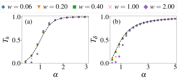
Figure 2: Bright soliton collisions with the geometric barrier $V_{h}$ [Eq. (2)] in the scalar GPE [Eq. (4)]. The plots show transmission as a function of $\alpha$ (ratio between velocity and barrier area, in units of $\hbar^{-1}$), for the barriers $V_{h}$ (a) and $V_{\delta}$ (b), and different values of the width $w$. Dashed lines in (a) and (b) show high-velocity limits for barriers $V_{\mathrm{RM}}$ and $V_{\delta}$, respectively.

We simulate the vector GPE [Eq. (1)] and scalar GPE [Eq. (4)] with periodic boundary conditions, corresponding to a quasi-1D ring trap configuration. We take ⁸⁵Rb with $\ket{g_{1}}=\ket{F=2,M_{F}-2}$ and $\ket{g_{2}}=\ket{F=2,M_{F}=0}$ coupled via the D1 line as an inspirational example. This has a wide Feshbach resonance around $B_{0}=156$ G Roberts et al. (1998); Blackley et al. (2013), which we use to tune $a_{11}\approx$-12\text{\,}\mathrm{\text{ $a_{0}$ }}$$, within the stable soliton region Cornish et al. (2006); Ruprecht et al. (1995); Roberts et al. (2001). Assuming all other scattering lengths to be equal to the background value $a_{\mathrm{bg}}=$-441\text{\,}\mathrm{\text{ $a_{0}$ }}$$ yields $g\approx 40$. To broaden our analysis, we vary $g$ between $-40$ and $40$. We work in “soliton” units of length $\hbar^{2}/m|g^{1\mathrm{D}}_{11}|N$, time $\hbar^{3}/m(g^{1\mathrm{D}}_{11}N)^{2}$, and energy $m(g^{1\mathrm{D}}_{11}N/\hbar)^{2}$ dim . Unless otherwise stated, we express quantities in these units, with total density normalized to 1. We set $l=2\sqrt{2}$ in our vector GPE simulations; for the above value of $a_{11}$, $N=2500$ and $\omega_{r}=2\pi\times$40\text{\,}\mathrm{Hz}$$, this corresponds to an SI value of $l=$2.7\text{\,}\mathrm{\SIUnitSymbolMicro m}$$ Wales et al. (2020). We assume an initial bright soliton $\psi_{1}=(1/2)\mathop{\mathrm{sech}([x+L/4]/2)}e^{ivx}$ in state $\ket{g_{1}}$, with $\psi_{2}=\psi_{e}=0$, and ring trap circumference $L=64\pi$.

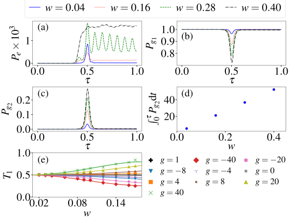
Figure 3: Bright soliton collisions with the proposed barrier configuration in the vector GPE [Eq. (1)]. (a–c) Populations as functions of time (in units of $\tau=L/2v$, the time over which the soliton moves from $-L/4$ to $L/4$) of states $\ket{e}$, $\ket{g_{1}}$, and $\ket{g_{2}}$, respectively. (d) Integrated time spent in state $\ket{g_{2}}$ as a function of $w$. In (a–d), we set $\Omega=10^{4}$ and $g=1$. (e) Transmission as a function of $w$ for different values of $g$, where we set $\Omega=10^{6}$, and fix incoming soliton velocities at values resulting in $T=0.5$ for scalar GPE simulations with $V_{h}$ barriers [Fig. 2 (a)]; solid lines show equivalent-parameter scalar GPE simulations with fully nonlinear barrier $V_{d}(x,|\psi_{d}|^{2})$ [Eq. (5)].

We first use the scalar GPE [Eq. (4)] to investigate soliton collisions with the squared-Lorentzian barrier $V_{h}$. We compare the total fraction of transmitted atoms $T$ with the analytic approximation for collisions with a same-height-and-area Rosen–Morse barrier, $V_{\mathrm{RM}}=[1/(2w^{2})]\mathop{\mathrm{sech}^{2}(4x/[\pi w])}$, in the high-velocity limit (neglecting the nonlinear term during the collision) Wales et al. (2020); Landau and Lifshitz (1959). We also compare indirectly to scalar GPE simulations with a same-area $\delta$-function barrier, $V_{d}=V_{\delta}(x)=[\pi/(4w)]\mathop{\delta(x)}$, which approach their own analytic high-velocity limit $T_{\delta}(\alpha)=\alpha^{2}/(1+\alpha^{2})$, where $\alpha=4vw/\pi$ is the rato between velocity and barrier area Holmer et al. (2007). Figure 2 shows numerical transmission curves for $V_{h}$ and $V_{\delta}$ barriers with different values of $w$ plotted against $\alpha$. As $w$ decreases, the transmission curves approach the analytic high-velocity limits for $V_{\mathrm{RM}}$ and $V_{\delta}$. How Fig. 2(a) and (b) differ illustrates an important point. Within an interferometer, an effective soliton beamsplitter should achieve $T=0.5$ in the tunneling regime, where the ratio $\gamma$ between per-atom kinetic energy and barrier height satisfies $\gamma<1$; the outgoing soliton velocities may otherwise have significantly different magnitudes owing to velocity filtering Wales et al. (2020). As collision velocities increase, we need decreasing barrier widths to remain in the tunneling regime Polo and Ahufinger (2013); Manju et al. (2018); Helm et al. (2014). The $V_{h}$ barrier width $w$ and area $\pi/(4w)$ are intrinsically inversely related, fixing the ratio $\gamma=(vw)^{2}=\left(\pi/4\right)^{2}\alpha^{2}$. Assuming $T=0.5$ occurs close to $\alpha=1$, $\gamma$ tends towards $(\pi/4)^{2}\approx 0.61$. The $\delta$-function limit $\gamma\rightarrow 0$ is therefore not attained with the $V_{h}$ barrier; as the width decreases with increasing ratio $\Omega_{1}/\Omega_{0}$, the velocity at which $T=0.5$ is nonetheless within the $\gamma<1$ tunneling regime. In Fig. 3 we investigate these same collisions using the vector GPE description [Eq. (1)] for varying $w$. We fix incoming soliton velocities at values resulting in $T=0.5$ for the scalar GPE with $V_{d}=V_{h}$ [Fig. 2(a)]. In Fig. 3(a–d) we consider equal scattering lengths ($g=1$) and characterize internal state populations as functions of time during the collision, showing the integrated time spent in state $\ket{g_{2}}$ as a function of $w$ in (d). As expected, decreasing $w$ generally reduces the populations of $\ket{g_{2}}$ and $\ket{e}$ and increases that of $\ket{g_{1}}$; the integrated time spent in state $\ket{g_{2}}$ also decreases. In Fig. 3(e) we show the transmission $T$ as a function of $w$ for a range of scattering length ratios $g$; as $w$ decreases, the effects of $g\neq 1$ reduce. The solid lines in Fig. 3(e) show results of the scalar GPE with fully nonlinear $V_{d}(x,|\psi_{d}|^{2})$ [Eq. (5)], which clearly matches the vector GPE well over the range of $g$ we explore.

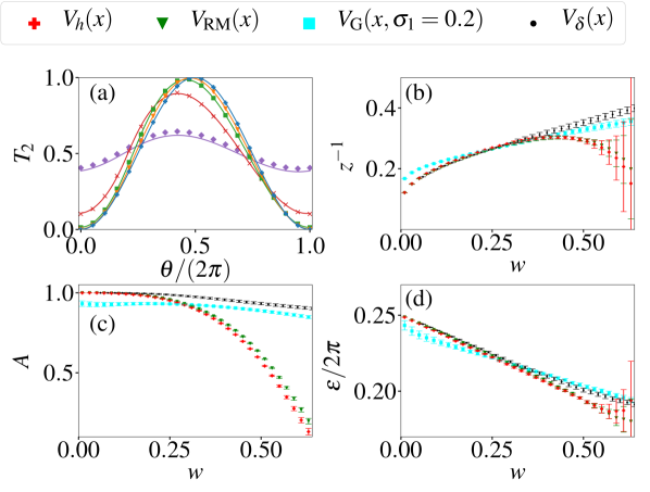
Figure 4: Bright soliton interferometry with the geometric barrier $V_{h}$ in the scalar GPE. (a) Transmission at recombination $T_{2}$ against imposed phase $\theta$ for $w=0.01$ (blue plus), $w=0.1$ (orange triangle), $w=0.2$ (green cross), $w=0.4$ (red square), and $w=0.6$ (purple diamond). (b)–(d) Fitted values [using Eq. (6)] of $z^{-1}$, $A$, and $\varepsilon$, respectively, for $V_{h}$ and for the alternative barrier shapes $V_{\mathrm{RM}}$, $V_{\delta}$, and $V_{\mathrm{G}}(\sigma=0.2)$ (see text) for varying $w$.

While various interferometric configurations are possible, we consider a conceptually simple quasi-1D ring trap with a single barrier. The barrier splits a single soliton into two equal-amplitude, equal-speed counterpropagating daughter solitons, which pass through one another and subsequently phase-sensitively recombine at the same barrier Helm et al. (2015). Imposing a relative phase $\theta$ between the daughter solitons, the fraction of atoms recombined to one side of the barrier should vary sinusoidally with $\theta$ in the high velocity and narrow barrier limit (i.e., $w\rightarrow 0$). We otherwise expect a nonlinearity-induced “skew” in the sinusoidal dependence Helm et al. (2012), and employ (generalized) Clausen functions $S_{z}(\theta)$ to empirically parametrize this effect. We fit the final population on the “transmitted” side of the barrier after the second collision (the recombination) with

$$T_{2}(\theta)=\frac{1}{2}\left[1+A\mathop{S_{z}(\theta-\varepsilon)}\right],$$ (6)

which ranges from a sawtooth function ($z=1$) to a sinusoid ($z\rightarrow\infty$). To improve fitting convergence and ensure bounded limits, we fit and present results in terms of $z^{-1}$, where smaller $z^{-1}$ corresponds to less skew fit ; Virtanen et al. (2020). The phase shift $\varepsilon$ incorporates relative phases accumulated during barrier collisions and subsequent evolution, and $A$ is the contrast or “fringe visibility.” For a $\delta$-function barrier in the high-velocity limit $z^{-1}\rightarrow 0$, $A=1$ and $\varepsilon=\pi/2$ Helm et al. (2012); Holmer et al. (2007). In Fig. 4 we show this limit is effectively reached with the $V_{h}$ barrier in the scalar GPE. We compare this scenario to the scalar GPE with alternative barriers $V_{d}=V_{\delta}(x)$, $V_{d}=V_{\mathrm{RM}}(x)$, and a narrow, fixed-width, Gaussian barrier with equal area to $V_{h}$: $V_{d}=V_{\mathrm{G}}(x;\sigma)=\{[\pi/(4w)]/[(2\pi)^{1/2}\sigma]\}\,\mathrm{exp}(-x^{2}/[2\sigma^{2}])$. For each data point a root-finding algorithm sets the initial velocity to achieve transmission $T=0.5$ at the first collision, and we model a range of imposed phases $\theta$. Figure 4(a) shows $T_{2}(\theta)$ for the $V_{h}$ barrier, directly illustrating the decrease in skew for decreasing $w$. Figures 4(b–d) show the values of $z^{-1}$, $A$, and $\varepsilon$ extracted by fitting Eq. (6) to the numerical simulations at width $w$. The $V_{h}$ barrier, and its Rosen–Morse approximant $V_{\mathrm{RM}}$, smoothly approach the ideal high-velocity $\delta$-function result of $A=1$ and $\varepsilon=\pi/2$ as $w\rightarrow 0$; note the fixed-width Gaussian barrier performs better at $w\gtrsim 0.3$, but cannot smoothly reach this result. The parameter $z^{-1}$ does not drop smoothly to zero, however at $z^{-1}<0.2$ the skew is barely resolved and the 3-parameter fit of Eq. (6) effectively over-fits in this limit.

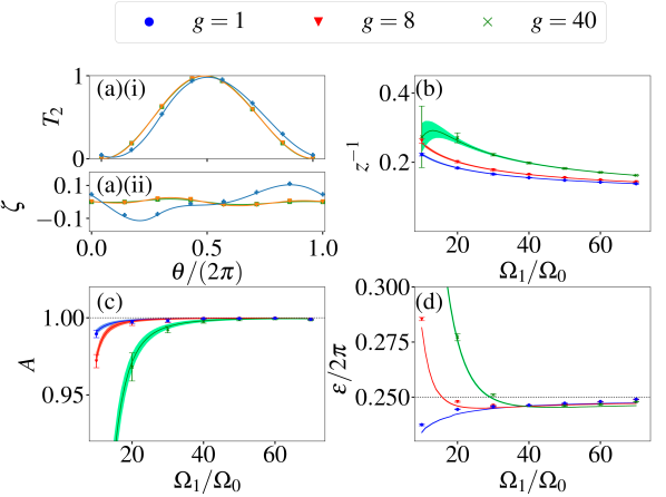
Figure 5: Bright soliton interferometry in the vector GPE [Eq. (1)]. (a)(i) Transmission at recombination $T_{2}$ against imposed phase $\theta$, and (a)(ii) difference from the ideal sinusoid $\zeta=T_{2}-(1/2)[1+\sin(\theta-\pi/2)]$, for $\Omega_{1}/\Omega_{0}=20$ (blue plus), $\Omega_{1}/\Omega_{0}=40$ (orange triangle), $\Omega_{1}/\Omega_{0}=60$ (green square), with $g=40$. (b)–(d) Values of $z^{-1}$, $A$, and $\varepsilon$, respectively, found by fitting with Eq. (6) for $g=1$, $g=8$, $g=40$. Solid lines show the fit to scalar GPE simulations with fully nonlinear barrier $V_{d}(x,|\psi|^{2})$ and equivalent parameters (shaded areas indicate error ranges). We use $\Omega=10^{4}$ for $\Omega_{1}/\Omega_{0}=$ 10, 20, 30 and $\Omega=5\times 10^{4}$ for $\Omega_{1}/\Omega_{0}=$ 40, 50, 60, 70 (see text).

In Fig. 5 we analyze the interferometer using the vector GPE [Eq. (1)] for $g=1,8,40$, presenting the results as functions of the ratio $\Omega_{1}/\Omega_{0}\equiv l/(2w)$. Due to the high computational demands of setting the initial velocities with our previously employed root-finding algorithm, we use values determined for Fig. 4 at equivalent widths $w$ for the $V_{h}$ barrier. In the ideal limit these velocities are the same, but otherwise significantly different $A$ and $\varepsilon$ values result for different $g$. Figure 5(a) shows directly the decrease in skew for $g=40$ as $\Omega_{1}/\Omega_{0}$ increases. Figure 5 (b–d) shows how the fit-extracted parameters $z^{-1}$, $A$, and $\varepsilon$ tend towards the ideal limit as $\Omega_{1}/\Omega_{0}$ increases. As in Fig. 3, solid lines show scalar GPE simulations with fully nonlinear potential $V_{d}(x,|\psi|^{2})$ (shaded areas indicate error ranges from fitting), again showing excellent agreement. We require high $\Omega$ values to keep internal state dynamics sufficiently fast relative to the collision duration as $\Omega_{1}/\Omega_{0}$ increases (values used are given in the figure caption). Extension to even higher $\Omega_{1}/\Omega_{0}$ values is in principle enabled by raising $\Omega$ further; the physically desirable strong separation of timescales makes this an increasingly challenging regime to fully simulate, however. Briefly considering off-resonant excitation and spontaneous decay, we similarly note that, in the desired regime of operation, the splitting at the barrier is a predominantly linear effect Holmer et al. (2007); Helm et al. (2012). Therefore, as an approximate model, we numerically solve the time-independent, three-state linear scattering problem for an incoming plane wave with wavenumber $k>0$ in state $\ket{g_{1}}$, and purely outgoing plane waves in every other channel. We include loss due to spontaneous decay from $|e\rangle$ by combining an imaginary term with the detuning, producing $-\Delta-i\Gamma/2$, where $\Gamma$ is the excited state linewidth. With ⁸⁵Rb parameters corresponding to the rightmost points in Fig. 5 (b–d), we find the effects of spontaneous decay and realistic detuning (equal to the linewidth) are negligible at the wavenumber $k$ required for equal splitting .

We have described a technique to create a single very narrow barrier for soliton interferometry using a geometric scalar potential Łącki et al. (2016); Jendrzejewski et al. (2016), based on two overlapping Hermite–Gaussian mode laser beams. We have used approximate scalar GPE and full vector GPE models to characterize both splitting and interferometric recombination at this barrier, demonstrating how to realize a very narrow effective barrier using moderately high laser intensity ratios. Critically, the initial equal splitting of a single soliton is then a tunneling rather than a velocity filtering process, and near-unit interferometric contrast is in principle achievable. We have also shown a scalar GPE with correctly chosen nonlinear barrier potential provides an excellent description of the system, provided the intensity of the weaker beam is sufficiently high. We hope this proposal will find practical application in the upcoming generation of matter-wave bright soliton experiments.

Additional data related to the findings reported in this paper is made available by source dat .

We thank S. L. Cornish, A. Guttridge, I. G. Hughes and A. Rakonjac for useful discussions. C.L.G. is supported by the UK EPSRC. This work made use of the Durham University Hamilton HPC Service.

References

- Strecker et al. (2002) K. E. Strecker, G. B. Partridge, A. G. Truscott, and R. G. Hulet, “Formation and propagation of matter-wave soliton trains,” Nature 417, 150 (2002).
- Khaykovich et al. (2002) L. Khaykovich, F. Schreck, G. Ferrari, T. Bourdel, J. Cubizolles, L. D. Carr, Y. Castin, and C. Salomon, “Formation of a matter-wave bright soliton,” Science 296, 1290 (2002).
- Cornish et al. (2006) S. L. Cornish, S. T. Thompson, and C. E. Wieman, “Formation of bright matter-wave solitons during the collapse of attractive Bose–Einstein condensates,” Phys. Rev. Lett. 96, 170401 (2006).
- Lepoutre et al. (2016) S. Lepoutre, L. Fouché, A. Boissé, G. Berthet, G. Salomon, A. Aspect, and T. Bourdel, “Production of strongly bound bright solitons,” Phys. Rev. A 94, 053626 (2016).
- Mežnaršič et al. (2019) T. Mežnaršič, T. Arh, J. Brence, J. Pišljar, K. Gosar, Ž Gosar, R. Žitko, E. Zupanič, and P. Jeglič, “Cesium bright matter-wave solitons and soliton trains,” Phys. Rev. A 99, 033625 (2019).
- Di Carli et al. (2019) Andrea Di Carli, Craig D. Colquhoun, Grant Henderson, Stuart Flannigan, Gian-Luca Oppo, Andrew J. Daley, Stefan Kuhr, and Elmar Haller, “Excitation modes of bright matter-wave solitons,” Phys. Rev. Lett. 123, 123602 (2019).
- (7) Strictly, such realizations are in the form of bright solitary waves, as the integrability conditions necessary for true solitons are formally not fully satisfied.
- Veretenov et al. (2007) N. Veretenov, Yu. Rozhdestvensky, N. Rosanov, V. Smirnov, and S. Federov, “Interferometric precision measurements with Bose–Einstein condensate solitons formed by an optical lattice,” Eur. Phys. J. D. 42, 455 (2007).
- Abdullaev and Brazhnyi (2012) F. Kh. Abdullaev and V. A. Brazhnyi, “Solitons in dipolar Bose-Einstein condensates with a trap and barrier potential,” J. Phys. B: At. Mol. Opt. Phys. 45, 085301 (2012).
- Martin and Ruostekoski (2012) A. D. Martin and J. Ruostekoski, “Quantum dynamics of atomic bright solitons under splitting and recollision, and implications for interferometry,” New J. Phys. 14, 043040 (2012).
- Helm et al. (2012) J. L. Helm, T. P. Billam, and S. A. Gardiner, “Bright matter-wave soliton collisions at narrow barriers,” Phys. Rev. A 85, 053621 (2012).
- Polo and Ahufinger (2013) J. Polo and V. Ahufinger, “Soliton-based matter-wave interferometer,” Phys. Rev. A 88, 053628 (2013).
- Cuevas et al. (2013) J. Cuevas, P. G. Kevrekedis, B. A. Malomed, P. Dyke, and R. G. Hulet, “Interactions of solitons with a Gaussian barrier: splitting and recombination in quasi-one-dimensional and three-dimensional settings,” New J. Phys. 15, 063006 (2013).
- Helm et al. (2015) J. L. Helm, S. L. Cornish, and S. A. Gardiner, “Sagnac interferometry using bright matter-wave solitons,” Phys. Rev. Lett. 114, 134101 (2015).
- Sakaguchi and Malomed (2016) H. Sakaguchi and B. A. Malomed, “Matter-wave soliton interferometer based on a nonlinear splitter,” New J. Phys. 18, 025020 (2016).
- McDonald et al. (2014) G. D. McDonald, C. C. N. Kuhn, K. S. Hardman, S. Bennetts, P. J. Everitt, P. A. Altin, J. E. Debs, J. D. Close, and N. P. Robins, “Bright solitonic matter-wave interferometer,” Phys. Rev. Lett. 113, 013002 (2014).
- Haine (2018) S. A. Haine, “Quantum noise in bright soliton matterwave interferometry,” New J. Phys. 20, 033009 (2018).
- Nguyen et al. (2014) J. H. V. Nguyen, P. Dyke, D. Luo, B. A. Malomed, and R. G. Hulet, “Collisions of matter-wave solitons,” Nat. Phys. 10, 918 (2014).
- Wales et al. (2020) O. J. Wales, A. Rakonjac, T. P. Billam, J. L. Helm, S. A. Gardiner, and S. L. Cornish, “Splitting and recombination of bright-solitary-matter waves,” Commun. Phys. 3, 51 (2020).
- Marchant et al. (2013) A. L. Marchant, T. P. Billam, T. P. Wiles, M. M. H. Yu, S. A. Gardiner, and S. L. Cornish, “Controlled formation and reflection of a bright solitary matter-wave,” Nat. Commun. 4, 1865 (2013).
- Łącki et al. (2016) M. Łącki, M. A. Baranov, H. Pichler, and P. Zoller, “Nanoscale “dark state” optical potentials for cold atoms,” Phys. Rev. Lett. 117, 233001 (2016).
- Jendrzejewski et al. (2016) F. Jendrzejewski, S. Eckel, T. G. Tiecke, G. Juzeliūnas, G. K. Campbell, Liang Jiang, and A. V. Gorshkov, “Subwavelength-width optical tunnel junctions for ultracold atoms,” Phys. Rev. A 94, 063422 (2016).
- Ge and Zubairy (2020) W. Ge and M. S. Zubairy, “Dark-state optical potential barriers with nanoscale spacing,” Phys. Rev. A 101, 023403 (2020).
- Subhankar et al. (2019) S. Subhankar, P. Bienias, P. Titum, T-C. Tsui, Y. Wang, A. V. Gorshkov, S. L. Rolston, and J. V. Porto, “Floquet engineering of optical lattices with spatial features and periodicity below the diffraction limit,” New J. Phys. 21, 113058 (2019).
- Bienias et al. (2020) P. Bienias, S. Subhankar, Y. Wang, T-C. Tsui, F. Jendrzejewski, T. Tiecke, G. Juzeliūnas, L. Jiang, S. L. Rolston, J. V. Porto, and A. V. Gorshkov, “Coherent optical nanotweezers for ultracold atoms,” Phys. Rev. A 102, 013306 (2020).
- Tsui et al. (2020) T-C. Tsui, Y. Wang, S. Subhankar, J. V. Porto, and S. L. Rolston, “Realization of a stroboscopic optical lattice for cold atoms with subwavelength spacing,” Phys. Rev. A 101, 041603 (2020).
- Kapale and Agarwal (2010) K. T. Kapale and G. S. Agarwal, “Subnanoscale resolution for microscopy via coherent population trapping,” Opt. Lett. 35, 2792 (2010).
- Dum and Olshanii (1996) R. Dum and M. Olshanii, “Gauge structures in atom-laser interaction: Bloch oscillations in a dark lattice,” Phys. Rev. Lett. 76, 1788 (1996).
- Goldman et al. (2014) N. Goldman, G. Juzeliūnas, P. Öhberg, and I. B. Spielman, “Light-induced gauge fields for ultracold atoms,” Rep. Prog. Phys. 77, 126401 (2014).
- Zhao et al. (2020) Yang Zhao, Shaokai Wang, Wei Zhuang, and Tianchu Li, “Raman-laser system for absolute gravimeter based on 87Rb atom interferometer,” Photonics 7, 32 (2020).
- Arias et al. (2017) N. Arias, V. Abediyeh, S. Hamzeloui, and E. Gomez, “Low phase noise beams for Raman transitions with a phase modulator and a highly birefringent crystal,” Opt. Express 25, 5290 (2017).
- Rosi et al. (2014) G. Rosi, F. Sorrentino, L. Cacciapuoti, M. Prevedelli, and G. M. Tino, “Precision measurement of the Newtonian gravitational constant using cold atoms,” Nature 510, 518 (2014).
- Meyrath et al. (2005) T. P. Meyrath, F. Schreck, J. L. Hanssen, C. S. Chuu, and M. G. Raizen, “A high frequency optical trap for atoms using Hermite–Gaussian beams,” Opt. Express 13, 2843 (2005).
- Zupancic et al. (2016) Philip Zupancic, Philipp M. Preiss, Ruichao Ma, Alexander Lukin, M. Eric Tai, Matthew Rispoli, Rajibul Islam, and Markus Greiner, “Ultra-precise holographic beam shaping for microscopic quantum control,” Opt. Express 24, 13881 (2016).
- Uehlinger et al. (2013) Thomas Uehlinger, Gregor Jotzu, Michael Messer, Daniel Greif, Walter Hofstetter, Ulf Bissbort, and Tilman Esslinger, “Artificial graphene with tunable interactions,” Phys. Rev. Lett. 111, 185307 (2013).
- Gati et al. (2006) R. Gati, M. Albiez, J. Fölling, B. Hemmerling, and M. K. Oberthaler, “Realization of a single Josephson junction for Bose–Einstein condensates,” App. Phys. B 82, 207 (2006).
- Malomed and Tasgal (1998) B. A. Malomed and R. S. Tasgal, “Internal vibrations of a vector soliton in the coupled nonlinear Schrödinger equations,” Phys. Rev. E 58, 2564 (1998).
- Manakov (1974) S. V. Manakov, “On the theory of two-dimensional stationary self-focussing of electromagnetic waves,” Sov. Phys. JETP 38, 248 (1974), [Zh. Eksp. Teor. Fiz. 65 505, (1974)].
- Roberts et al. (1998) J. L. Roberts, N. R. Claussen, J. P. Burke, C. H. Greene, E. A. Cornell, and C. E. Wieman, “Resonant magnetic field control of elastic scattering in cold 85Rb,” Phys. Rev. Lett. 81, 5109 (1998).
- Blackley et al. (2013) C. L. Blackley, C. R Le Sueur, J. M. Hutson, D. J. McCarron, M. P. Köppinger, H. W. Cho, D. L. Jenkin, and S. L. Cornish, “Feshbach resonances in ultracold 85Rb,” Phys. Rev. A 87, 033611 (2013).
- Ruprecht et al. (1995) P. A. Ruprecht, M. J. Holland, K. Burnett, and M. Edwards, “Time-dependent solution of the nonlinear Schrödinger equation for Bose-condensed trapped neutral atoms,” Phys. Rev. A 51, 4704 (1995).
- Roberts et al. (2001) J. L. Roberts, N. R. Claussen, S. L. Cornish, E. A. Donley, E. A. Cornell, and C. E. Wieman, “Controlled collapse of a Bose–Einstein condensate,” Phys. Rev. Lett. 86, 4211 (2001).
- (43) Heuristically this can be expressed as .
- Landau and Lifshitz (1959) L. D. Landau and E. M. Lifshitz, Quantum Mechanics (Non-Relativistic Theory) (Pergamon, 1959).
- Holmer et al. (2007) J. Holmer, J. Marzuola, and M. Zworski, “Fast soliton scattering by delta impurities,” Commun. Math. Phys. 274, 187 (2007).
- Manju et al. (2018) P. Manju, K. S. Hardman, M. A. Sooriyabandara, P. B. Wigley, J. D. Close, N. P. Robins, M. R. Hush, and S. S. Szigeti, “Quantum tunneling dynamics of an interacting Bose–Einstein condensate through a Gaussian barrier,” Phys. Rev. A 98, 053629 (2018).
- Helm et al. (2014) J. L. Helm, S. J. Rooney, C. Weiss, and S. A. Gardiner, “Splitting bright matter-wave solitons on narrow potential barriers: quantum to classical transition and applications to interferometry,” Phys. Rev. A 89, 033610 (2014).
- (48) In detail, using scipy.optimize.curve_fit Virtanen et al. (2020), we perform a least-squares fit to the numerical data assuming equal uncertainty in each data point, and plot one standard deviation uncertainties in the fit parameters obtained from the covariance matrix after scaling the minimized reduced statistic to .
- Virtanen et al. (2020) P. Virtanen, R. Gommers, T. E. Oliphant, M. Haberland, T. Reddy, D. Cournapeau, E. Burovski, P. Peterson, W. Weckesser, J. Bright, S. J. van der Walt, M. Brett, J. Wilson, K. J. Millman, N. Mayorov, A. R. J. Nelson, E. Jones, R. Kern, E. Larson, C. J. Carey, İ. Polat, Y. Feng, E. W. Moore, J. VanderPlas, D. Laxalde, J. Perktold, R. Cimrman, I. Henriksen, E. A. Quintero, C. R. Harris, A. M. Archibald, A. H. Ribeiro, F. Pedregosa, P. van Mulbregt, and SciPy 1.0 Contributors, “SciPy 1.0: Fundamental Algorithms for Scientific Computing in Python,” Nature Methods 17, 261 (2020).
- Note (1) Specifically, the wavenumber required for equal splitting shifts by %, and % of the incoming atom flux is lost at this wavenumber.
- (51) “Data are available through Durham University data management,” DOI:10.15128/r11j92g749r.