Multimode parity-time and loss-compensation symmetries in coupled waveguides with loss and gain

Abstract

Loss compensation via inserting gain is of fundamental importance in different branches of photonics, nanoplasmonics, and metamaterial science. This effect has found an impressive implementation in the parity-time symmetric ($\mathcal{PT}$-symmetric) structures possessing balanced distribution of loss and gain. In this work, we generalize this phenomenon to the asymmetric systems demonstrating loss compensation in the coupled multi-mode loss-gain dielectric waveguides of different radii. We show that similar to the $\mathcal{PT}$-symmetric coupled single-mode waveguides of identical radii, the asymmetric systems support the exceptional points called here the loss compensation (LC) thresholds where the frequency spectrum undergoes a transition from complex to real values. Moreover, the LC-symmetry thresholds can be obtained for dissimilar modes excited in the waveguides providing an additional degree of freedom to control the system response. In particular, changing loss and gain of asymmetric coupled waveguides, we observe loss compensation for TM and TE modes as well as for the hybrid HE and EH modes.

I Introduction

The intriguing properties of loss-gain distributions are the subject of the fast-growing field of non-Hermitian photonics. The most notable and studied class of non-Hermitian systems is the $\mathcal{PT}$-symmetric systems which possess the perfectly balanced spatial distribution of gain and loss [1, 2, 3]. $\mathcal{PT}$ symmetry guarantees the reality of non-Hermitian Hamiltonian spectra [4] that have been readily implemented and observed in the optical domain [5, 6]. Subsequently, $\mathcal{PT}$ symmetry was transferred to electronic circuits [7], acoustics [8], and time-varying (Floquet) systems [9].

The balance between loss and gain helps to solve the problem of loss compensation which is of paramount importance for the efficiency of plasmonic and metamaterial-based devices [10, 11, 12]. The loss compensation effect proved to be connected to another remarkable feature of non-Hermitian systems – the possibility of specific degeneracies called exceptional points (EPs) which were observed in photonics [13, 14] as well as in acoustics [15]. In contrast to the degeneracies of Hermitian systems (the so-called diabolic points) with coalescing eigenvalues, the EPs imply coalescence of both eigenvalues and eigenfunctions. In the $\mathcal{PT}$-symmetric systems, the EPs mark the points of phase transitions between the $\mathcal{PT}$-symmetric phase and the phase with spontaneously broken $\mathcal{PT}$ symmetry. It is important to emphasize, however, that the EPs are the general phenomenon observed also in purely passive systems (such as whispering-gallery-mode microresonators [16], ring cavities [17], and anisotropic waveguides [18]) and even in the systems with radiative loss only [19].

The EPs have become a workhorse of many recent achievements such as enhanced perturbation sensing [20, 21], novel lasing schemes [22, 23], enhanced Sagnac effect for laser gyroscopes [24, 25], simultaneous coherent perfect absorption and amplification [26, 27], asymmetric transmission [5, 28], etc. An interesting feature of EPs is their topological nature which can be revealed with their dynamical encircling in parameter space and can be used for mode switching [29], mode transfer [30], and polarization conversion [31]. Another exciting direction is the observation and utilization of the higher-order EPs, where more than two eigenmodes coalesce. Such EPs can be realized either in the systems containing three or more resonant elements [21, 32, 33] or by hybridizing several usual (second-order) EPs [34, 35]. It should be noted that the most considerations of non-Hermitian effects are limited to the single-mode case with the use of the coupled-mode theory (CMT) [36]. The multi-mode platforms provide much richer opportunities in controlling optical response and dynamics as evidenced by the examples of dispersion engineering and mode conversion in the waveguide and microresonator systems [37, 38, 39].

For the symmetric system of coupled dielectric waveguides, the full loss compensation is possible only for the perfect balance between gain and loss corresponding to the non-violated $\mathcal{PT}$-symmetry [6]. This poses rather tough and difficult-to-achieve conditions for experimental realization of the related effects [13]. On the contrary, for the asymmetric system, the full loss compensation can be reached even for the unbalanced gain and loss. By analogy with the $\mathcal{PT}$-symmetry, this generalized situation can be called the loss-compensation (LC) symmetry [40, 41]. In this paper, we propose further generalization demonstrating LC symmetry for the coupled dissimilar waveguides under excitation of the modes with the same or different azimuthal indices. In dielectric waveguides, all modes except TE and TM are hybrid, i.e., they have axial components of both electric and magnetic fields. Therefore, to analyze the system, we apply the multi-mode approach [42, 41] which allows us to obtain exact solutions of the eigenvalue problem for all possible classes of modes supported by the asymmetric guiding structure. We show that such an asymmetric structure supports specific EPs called the LC-symmetry thresholds and reached for different loss-gain ratios depending on the modes used. Thus, the mode composition of the non-Hermitian system is an additional degree of freedom useful for tuning the parameters necessary to obtain the constant-intensity modes [43, 44] and other applications.

II Multimode analytical approach

For our analysis, we use the multi-mode analytical approach [42], which was previously successfully applied to coupled systems with loss and gain [41]. Following Ref. [41], we consider a pair of coupled dielectric cylinders of the radii $R_{1}$ and $R_{2}$ placed in an ambient medium. Figure 1 shows the cross-sections of the dielectric circular waveguides with the permittivities $\varepsilon_{1}$ and $\varepsilon_{2}$, respectively (Regions I and II). The polar coordinate systems associated with the waveguides are denoted as ($r_{1},\phi_{1}$) and ($r_{2},\phi_{2}$). The waveguides are placed in the infinite uniform medium (Region III) with the real permittivity $\varepsilon_{3}\in\Re$. The permeability $\mu=\mu_{0}$ is assumed to be the same in all regions. Without loss of generality, we suppose that the first waveguide contains gain material and the second one contains lossy medium (Im$(\varepsilon_{1})<0$ and Im$(\varepsilon_{2})>0$), whereas Re$(\varepsilon_{1})>\varepsilon_{3}$ and Re$(\varepsilon_{2})>\varepsilon_{3}$.

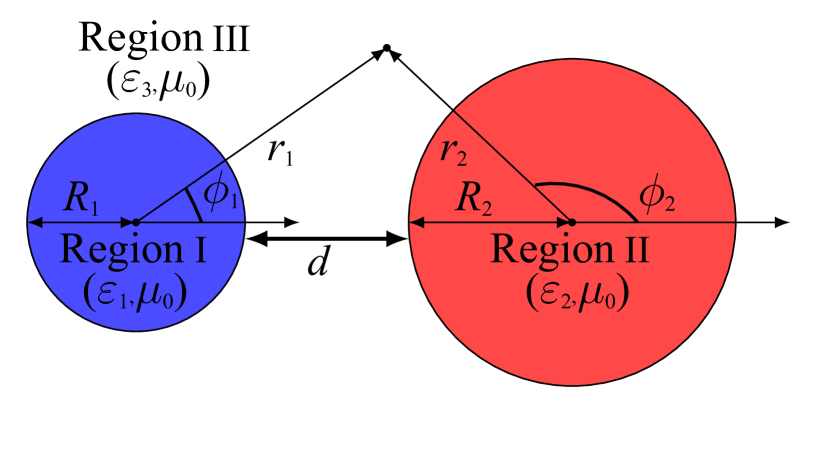
Figure 1: Geometry of unequally sized dielectric waveguides immersed in an infinite medium.

In order to solve the eigenvalue problem for this system, we write the electromagnetic fields in every region using the corresponding polar coordinates as shown in Fig. 1. For example, the $E_{z}$ and $H_{z}$ components of electromagnetic fields in the Region I are written in terms of the local coordinates $(r_{1},\phi_{1})$ as

$$\begin{split}E_{z}^{1}&=\sum_{n=-N}^{N}{A_{n}^{1}J_{n}(k_{p,1}r_{1})e^{in\phi_{1}}},\\ H_{z}^{1}&=\sum_{n=-N}^{N}{B_{n}^{1}J_{n}(k_{p,1}r_{1})e^{in\phi_{1}}},\end{split}$$ (1)

whereas in the Region II the local coordinates $(r_{2},\phi_{2})$ are used as

$$\begin{split}E_{z}^{2}&=\sum_{n=-N}^{N}{A_{n}^{2}J_{n}(k_{p,2}r_{2})e^{in\phi_{2}}},\\ H_{z}^{2}&=\sum_{n=-N}^{N}{B_{n}^{2}J_{n}(k_{p,2}r_{2})e^{in\phi_{2}}},\end{split}$$ (2)

and, finally, in the Region III we have the contributions from both local coordinate systems,

$$\begin{split}E_{z}^{3}=&\sum_{n=-N}^{N}{C_{n}^{1}H_{n}^{(1,2)}(k_{p,3}r_{1})e^{in\phi_{1}}}\\ &+\sum_{n=-N}^{N}{C_{n}^{2}H^{(1,2)}_{n}(k_{p,3}r_{2})e^{in\phi_{2}}},\\ H_{z}^{3}=&\sum_{n=-N}^{N}{D_{n}^{1}H^{(1,2)}_{n}(k_{p,3}r_{1})e^{in\phi_{1}}}\\ &+\sum_{n=-N}^{N}{D_{n}^{2}H^{(1,2)}_{n}(k_{p,3}r_{2})e^{in\phi_{2}}}.\end{split}$$ (3)

Here $\{A_{n}^{1},A_{n}^{2},B_{n}^{1},B_{n}^{2},C_{n}^{1},C_{n}^{2},D_{n}^{1},D_{n}^{2}\}$ are the unknown amplitudes of azimuthal harmonics, $k_{p,i}^{2}=k^{2}_{i}-k_{z}^{2}$, $k_{i}=k_{0}\varepsilon_{r_{i}}$ $(i=1,2,3)$, $\varepsilon_{r_{i}}=\varepsilon_{i}/\varepsilon_{0}$ is the relative permittivity, $k_{0}^{2}=\omega^{2}\varepsilon_{0}\mu_{0}$, $J_{n}(\cdot)$ is the Bessel function, $H_{n}^{(1)}(\cdot)$ and $H_{n}^{(2)}(\cdot)$ are the Hankel functions of the first and second kind, respectively, and the field factor of the form $\exp{[-i(\omega t-k_{z}z)]}$ is assumed and omitted. The choice of the Hankel function is governed by the boundary conditions for the fields in the Region III, as follows: $E_{z}^{3}\rightarrow 0$ and $H_{z}^{3}\rightarrow 0$ for $r_{1},r_{2}\rightarrow\infty$.

Since the derivation of other field components is cumbersome, it is relegated to the Appendix. We only note that the Maxwell equations and Eqs. (1)-(3) allow us to obtain the expressions for the electromagnetic field components $E_{\phi}$ and $H_{\phi}$ in every Region. The unknown coefficients $\{A_{n}^{1},A_{n}^{2},B_{n}^{1},B_{n}^{2},C_{n}^{1},C_{n}^{2},D_{n}^{1},D_{n}^{2}\}$ and $k_{z}$ can be obtained from the dispersion relation derived using the continuity conditions for the tangential fields at the boundary surfaces $r_{1}=R_{1}$ and $r_{2}=R_{2}$ (see Appendix).

III TM and TE modes

III.1 Single waveguide modes

Our aim is to demonstrate the possibility of full loss compensation for the coupled dielectric waveguides with gain and loss supporting different modes with an arbitrary value of azimuthal index. The dispersion relations of coupled waveguides will tend to the dispersion relations of independent waveguides with increasing distance between them. Therefore, we are interested in the crossing points of the dispersion curves of two independent cylinders. The dispersion curves for the lowest-order modes of a single waveguide are shown in Fig. 2. Changing the radius or permittivity of another cylinder, one can observe the shift of its dispersion curves with respect to the curves of the first one. Thus, for any pair of modes, we can find their crossing points at a required frequency $f$ and longitudinal wavenumber $k_{z}/k_{0}$. We will show further that these crossing points are convenient for the realization of full loss compensation at the certain values of gain-loss parameter and distance between the cylinders.

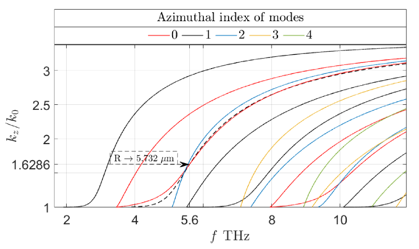
Figure 2: Lowest-order modes of the circular dielectric waveguide with $\epsilon_{r}=12$ and $R=10$ $\mu$m

Let us consider, for the moment, the family of transverse electric TE_0m and transverse magnetic TM_0m modes of the circular cylindrical waveguide. As representatives of these modes, we choose the set {TM₀₁, TM₀₂, TE₀₁, TE₀₂}. For example, for the TM₀₁ (TE₀₁) mode, we can choose an arbitrary solution of the dispersion relation ($f$; $k_{z}/k_{0}$). Then, we increase the cylinder radius to obtain same solution for the TM₀₂ (TE₀₂) mode. The initial and increased radii of the waveguide can serve as a first approximation to find the conditions of loss compensation for the coupled cylinders with gain and loss. For instance, according to Fig. 2, the values $f=5.6$ THz and $k_{z}/k_{0}=1.6286$ correspond to the TM₀₁ (TE₀₁) mode of the waveguide with $\epsilon_{r1}=12$ and $R_{1}=10$ $\mu$m and to the TM₀₂ (TE₀₁) mode of the waveguide with $\epsilon_{r2}=12$ and $R_{2}=18.93$ $\mu$m ($R_{2}=16.305$ $\mu$m).

III.2 Symmetric coupled waveguides: $\mathcal{PT}$ symmetry

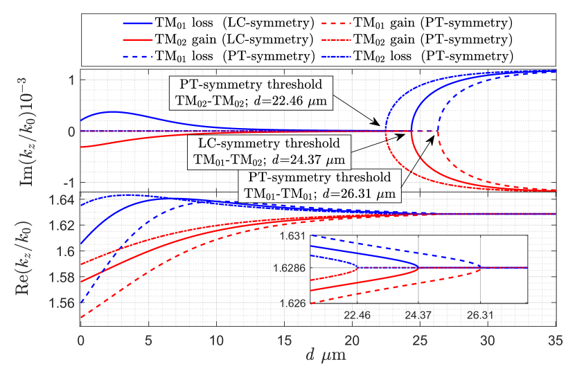
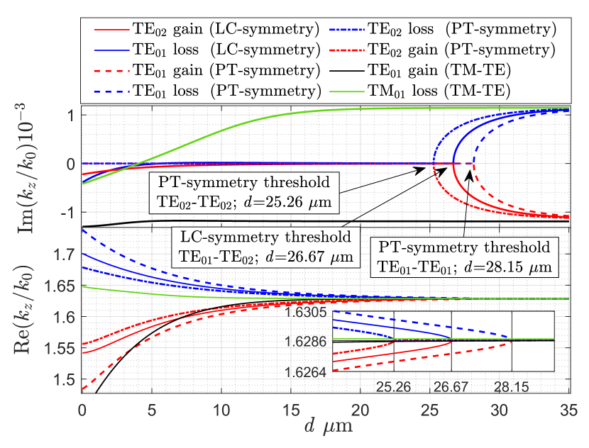
Figure 3: The real and imaginary parts of the eigenvalues $k_{z}/k_{0}$ for the TM modes as a function of the distance $d$ between the coupled waveguides. LC- and $\mathcal{PT}$-symmetry thresholds of TM-type modes are shown with arrows.

Figure 4: The real and imaginary parts of the eigenvalues $k_{z}/k_{0}$ for the TE modes as a function of the distance $d$ between the coupled waveguides. LC- and $\mathcal{PT}$-symmetry thresholds of TM-type modes are shown with arrows.

We start with the case of symmetric system consisting of the coupled waveguides with the same radii and permittivities, i.e., $R_{1}=R_{2}$ and $\epsilon_{r1}=\epsilon_{r2}$. In the case of balanced loss and gain, when the loss tangents have the same absolute value, $\tan{\delta_{1}}=-\tan{\delta_{2}}$, this system is a $\mathcal{PT}$-symmetric one. $\mathcal{PT}$-symmetric systems can exist in two states: a $\mathcal{PT}$-symmetric state with the loss exactly compensated by gain, and the broken-$\mathcal{PT}$-symmetry state with the violated compensation. In our case, the transition between these states can be realized by changing the distance between the cylinders. The point of transition where the $\mathcal{PT}$ symmetry gets broken is the EP, where the modes of the system are degenerate. For example, in Fig. 4, the dashed and dash-dotted lines correspond to the TM₀₁ and TM₀₂ modes of the coupled waveguides with balanced gain and loss (the parameters are $R_{1}=R_{2}=10$ $\mu$m, $\epsilon_{r1}=\epsilon_{r2}=12$, $\tan{\delta_{1}}=-\tan{\delta_{2}}=5\cdot 10^{-4}$ for TM₀₁ and $R_{1}=R_{2}=18.93$ $\mu$m, $\epsilon_{r1}=\epsilon_{r2}=12$, $\tan{\delta_{1}}=-\tan{\delta_{2}}=4.05\cdot 10^{-4}$ for TM₀₂), whereas in Fig. 4, the dashed and dash-dotted lines correspond to the TE₀₁ and TE₀₂ modes of the system with another set of parameters ($R_{1}=R_{2}=7.48$ $\mu$m, $\epsilon_{r1}=\epsilon_{r2}=12$, $\tan{\delta_{1}}=-\tan{\delta_{2}}=5\cdot 10^{-4}$ for TE₀₁ and $R_{1}=R_{2}=16.305$ $\mu$m, $\epsilon_{r1}=\epsilon_{r2}=12$, $\tan{\delta_{1}}=-\tan{\delta_{2}}=4.09\cdot 10^{-4}$ for TE₀₂, respectively). The EPs are denoted as the $\mathcal{PT}$-symmetry thresholds, since below these points (for distances smaller than the threshold one) the eigenvalues $k_{z}/k_{0}$ become purely real and the system falls into the $\mathcal{PT}$-symmetric state. This state is preserved to the very connection of the cylinders at $d=0$. It is important to note that due to the symmetry of the system, the full loss compensation via the $\mathcal{PT}$-symmetric state formation is observed only for the identical modes of both waveguides.

III.3 Asymmetric coupled waveguides: LC symmetry

Although $\mathcal{PT}$-symmetric systems allow perfect loss compensation, it is often problematic to reach the ideal symmetry and the ideal loss-gain balance in realistic situations. Here, we show that loss compensation can be obtained in asymmetric systems with unequal coupled waveguides. Such situation can be described as LC symmetry [40], which has much in common with $\mathcal{PT}$ symmetry (e.g., the existence of EPs), but at the same time, the requirements for system symmetry are strongly relaxed. Moreover, LC symmetry is reached for a pair of different modes as will be illustrated further.

Let us take the loss tangent of the first cylinder equal to $\tan{\delta_{1}}=5\cdot 10^{-4}$ corresponding to the value for silicon [45]. Changing the gain tangent $\tan{\delta_{2}}$ and the distance between the cylinders $d$, we can obtain the full loss compensation at the target frequency $f=5.6$ THz and wavenumber $k_{z}/k_{0}=1.6286$. For the TE₀₁ and TE₀₂ modes, the EP which we call the LC-symmetry threshold is reached at the system parameters as follows: $R_{1}=7.48$ $\mu$m, $R_{2}=16.305$ $\mu$m, $\epsilon_{r1}=\epsilon_{r2}=12$, $d=26.67$ $\mu$m, $\tan{\delta_{2}}=-4.05\cdot 10^{-4}$) (see Fig. 5, green and black lines). For the modes TM₀₁ and TM₀₂, the EP is reached at $d=24.37$ $\mu$m and $\tan{\delta_{2}}=-4.05\cdot 10^{-4}$ (see Fig. 5, blue and red lines). Similarly to the $\mathcal{PT}$-symmetry threshold, the LC-symmetry threshold corresponds to the purely real eigenvalues $k_{z}/k_{0}$. This approach can be utilized to obtain the EPs of full loss compensations for other pairs of modes as well.

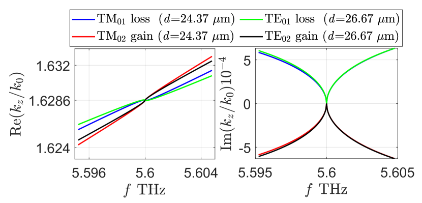
Figure 5: EPs corresponding to the LC symmetry for the pairs of modes TM₀₁-TM₀₂ and TE₀₁-TE₀₂.

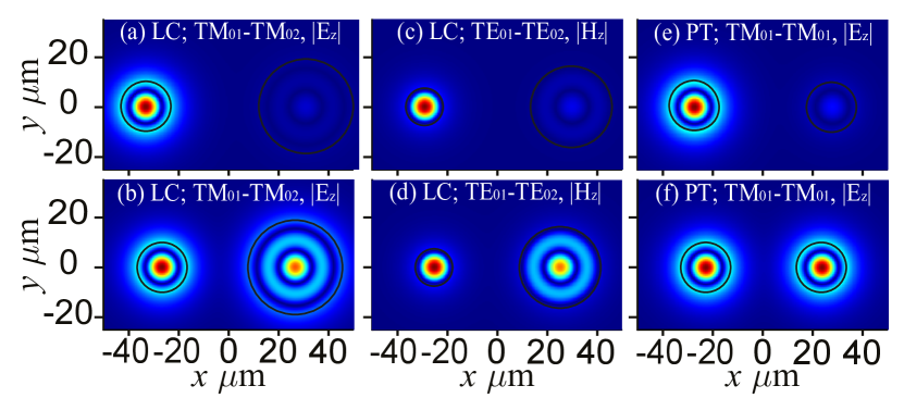
Figure 6: (a), (c) Electric $|E_{z}|$ and Magnetic $|H_{z}|$ field components corresponding to the broken LC-symmetry case for TM₀₁ and TE₀₁ loss modes at distance $d=35~{}\mu$m. (b), (d) Electric $|E_{z}|$ and Magnetic $|H_{z}|$ field components corresponding to the LC-symmetry thresholds of TM₀₁-TM₀₂ and TE₀₁-TE₀₂ mode pairs at distances $d=24.37~{}\mu$m and $d=26.67~{}\mu$m. (e), (f) Electric field $|E_{z}|$ corresponding to the asymmetry and $\mathcal{PT}$-symmetry cases of TM₀₁-TM₀₁ mode pairs at distances $d=35~{}\mu$m and $d=26.31~{}\mu$m.

In Figs. 4 and 4, the LC-symmetry thresholds are shown for the TM-type and TE-type modes, respectively, and compared to the $\mathcal{PT}$-symmetry thresholds. One can see that the LC-symmetry thresholds for the different modes (for example, TM₀₁ and TM₀₂) lie between the $\mathcal{PT}$-symmetry thresholds for the corresponding individual modes. The main difference with the $\mathcal{PT}$-symmetric case is that the eigenvalues for the asymmetric waveguides do not remain real below the LC-symmetry threshold. In fact, full loss compensation is realized only in a single point. The position of this point – LC-symmetry threshold – depends on the loss tangent and the frequency at which the dispersion curves cross. An example of electric and magnetic field distributions at the LC-symmetry threshold and dots of broken symmetry for dissimilar waveguides are shown in Figs. 6(b) and 6(d) and Figs. 6(a) and 6(c) as compared to the distributions at the $\mathcal{PT}$-symmetry thresholds and case of broken $\mathcal{PT}$-symmetry for the identical waveguides in Fig. 6(f) and 6(e). The smaller the loss tangent and the nearer the crossing to the cutoff frequency, the larger the distance between the waveguides corresponding to the threshold [41].

Thus, the LC-symmetry threshold in the asymmetric system allows one to fully compensate the loss for the unbalanced gain and loss of the individual cylinders. This effect can be considered as a generalization of $\mathcal{PT}$-symmetric loss compensation, since both the dispersion curves and the behavior of electromagnetic fields show that the nature of loss compensation phenomenon in asymmetric systems is similar to the $\mathcal{PT}$ symmetry in symmetric ones.

IV Hybrid modes: LC-symmetry

IV.1 Modes with the same azimuthal index

We have shown above how LC and $\mathcal{PT}$ symmetries can be observed by coupling either TM or TE modes of the pair of cylindrical waveguides. However, when one mode is TM one and another is TE one, we cannot obtain an EP due to the weak coupling between the modes of different types (see Fig. 4, green and pink lines). In order to get around this problem, in this section, we consider the possibility of LC symmetry for the hybrid modes, which can be treated as a linear superposition of the corresponding TE and TM modes. These modes having both the electric and magnetic field components in the longitudinal direction can be either of HE type (magnetic component dominates) or EH type (electric component dominates).

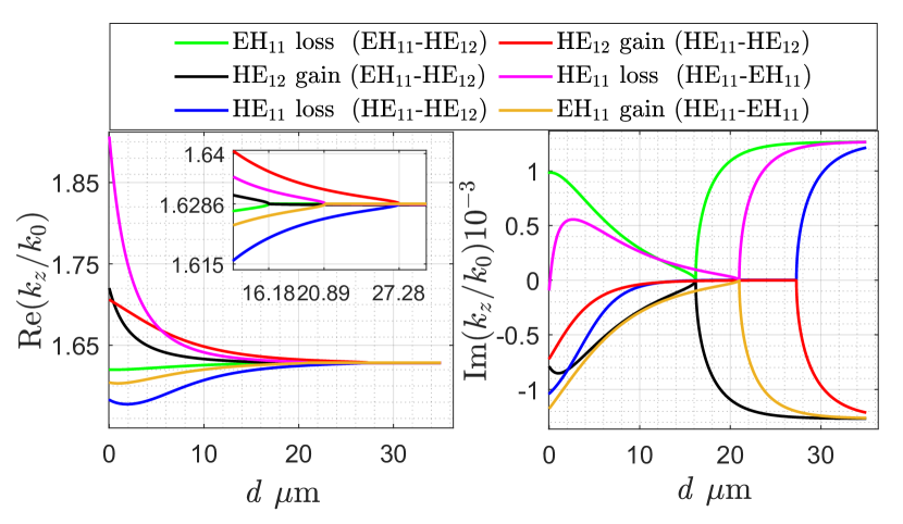
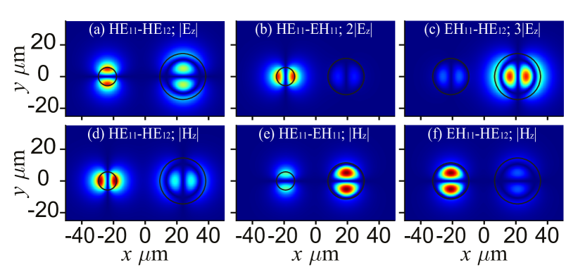
Figure 7: LC symmetry for the hybrid modes with the azimuthal index $1$.

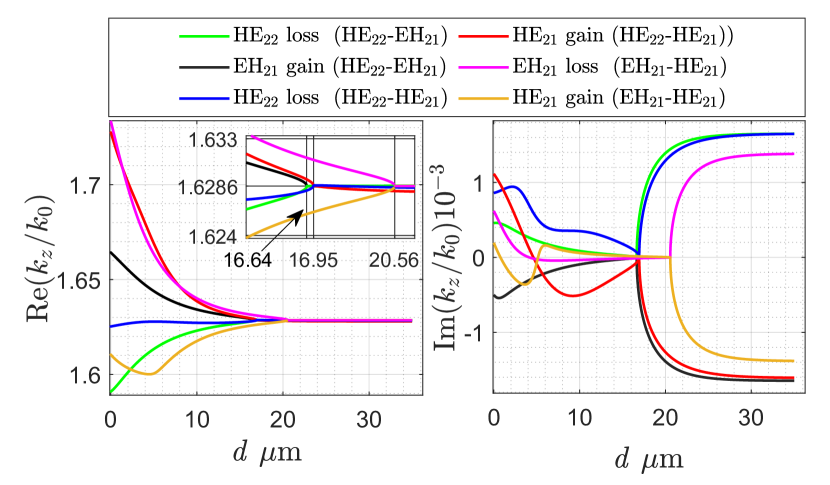
Figure 8: (a), (b), (c) Electric field $|E_{z}|$ corresponding to the LC-symmetry thresholds of HE₁₁-HE₁₂, HE₁₁-EH₁₁ and EH₁₁-HE₁₂ mode pairs; (d), (e), (f) The corresponding magnetic field $|H_{z}|$.

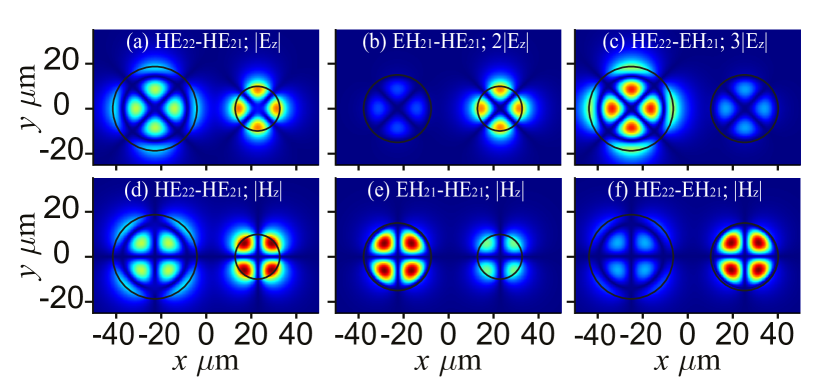
Figure 9: LC-symmetry of hybrid modes with the azimuthal index $2$.

Figure 10: (a), (b), (c) Electric field $|E_{z}|$ corresponding to the LC-symmetry thresholds of HE₂₂-HE₂₁, EH₂₁-HE₂₁ and HE₂₂-EH₂₁ mode pairs; (d), (e), (f) The corresponding magnetic field $|H_{z}|$.

We tune the dispersion curves for two cylinders to obtain the LC-symmetry thresholds of hybrid modes for the same parameters ($f=5.6$ THz and $k_{z}/k_{0}=1.6286$) as for the TM and TE modes. As previously, we start from the modes of the individual waveguide and shift the dispersion curves by changing the radius to get the required mode at the target frequency and wavenumber. For example, we obtain the hybrid mode HE₁₁ at $f=5.6$ THz and $k_{z}/k_{0}=1.6286$ for the cylinder with $R=5.732$ $\mu$m (see Fig. 2, dashed line).

Let us consider the class of hybrid modes with azimuthal index $1$ focusing in particular on the modes HE₁₁, EH₁₁ and HE₁₂ (see Fig. 2, black lines). We are interested in the LC symmetry between the mode pairs HE₁₁-EH₁₁, HE₁₁-HE₁₂ and EH₁₁-HE₁₂ with the first mode corresponding to the cylinder with loss (Region I) and the second mode corresponding to the cylinder with gain (Region II). As shown in Fig. 10, the LC-symmetry thresholds exist for all the mode pairs mentioned above and for the system parameters as follows:

• HE₁₁-EH₁₁ – {$R_{1}=5.732$ $\mu$m, $R_{2}=11.44$ $\mu$m, $\epsilon_{r1}=\epsilon_{r2}=12$, $\tan{\delta_{1}}=5\cdot 10^{-4}$, $\tan{\delta_{2}}=-4.91\cdot 10^{-4}$};

• HE₁₁-HE₁₂ – {$R_{1}=5.732$ $\mu$m, $R_{2}=14.487$ $\mu$m, $\epsilon_{r1}=\epsilon_{r2}=12$, $\tan{\delta_{1}}=5\cdot 10^{-4}$, $\tan{\delta_{2}}=-4.33\cdot 10^{-4}$};

• EH₁₁-HE₁₂ – {$R_{1}=11.44$ $\mu$m, $R_{2}=14.487$ $\mu$m, $\epsilon_{r1}=\epsilon_{r2}=12$, $\tan{\delta_{1}}=4.91\cdot 10^{-4}$, $\tan{\delta_{2}}=-4.33\cdot 10^{-4}$}.

We see that the LC-symmetry thresholds are reached for different distances between waveguides for every pair of modes: $d=20.89$ $\mu$m for HE₁₁-EH₁₁; $d=27.28$ $\mu$m for HE₁₁-HE₁₂; and $d=16.18$ $\mu$m for EH₁₁-HE₁₂. The field profiles shown in Fig. 10 prove that there are nonzero $E_{z}$ and $H_{z}$ in both cylinders as expected for the hybrid modes (although contribution of electric or magnetic field can strongly differ).

As to the hybrid modes with the azimuthal index $2$, we choose the mode pairs as follows: HE₂₂-EH₂₁, HE₂₂-HE₂₁ and EH₂₁-HE₂₁. Now, unlike previous cases, the radius of the waveguide with loss should be taken larger than the radius of the cylinder with gain. For the parameters of the corresponding LC-symmetry thresholds, shown in Figs. 10 and 10, we have:

• HE₂₂-EH₂₁ – {$R_{1}=18.7$ $\mu$m, $R_{2}=15$ $\mu$m, $\epsilon_{r1}=\epsilon_{r2}=12$, $\tan{\delta_{1}}=5\cdot 10^{-4}$, $\tan{\delta_{2}}=-5.95\cdot 10^{-4}$};

• HE₂₂-HE₂₁ – {$R_{1}=18.7$ $\mu$m, $R_{2}=9.91$ $\mu$m, $\epsilon_{r1}=\epsilon_{r2}=12$, $\tan{(\delta_{1})}=5\cdot 10^{-4}$, $\tan{(\delta_{2})}=-4.65\cdot 10^{-4}$};

• EH₂₁-HE₂₁ – {$R_{1}=15$ $\mu$m, $R_{2}=9.91$ $\mu$m, $\epsilon_{r1}=\epsilon_{r2}=12$, $\tan{\delta_{1}}=5\cdot 10^{-4}$, $\tan{\delta_{2}}=-4\cdot 10^{-4}$}.

The distances between the waveguides corresponding to these thresholds are: $d=16.64$ $\mu$m for HE₂₂-EH₂₁; $d=16.95$ $\mu$m for HE₂₂-HE₂₁; and $d=20.56$ $\mu$m for EH₂₁-HE₂₁. The results in Figs. 10-10 evidence that the full loss compensation can be realized for the arbitrary hybrid modes with the same azimuthal index. The structure of the modes influence only which of the cylinders should have larger radius – the lossy or the gainy one.

IV.2 Modes with different azimuthal indices

In this subsection, we study the possibility of LC symmetry in the coupled waveguides with loss and gain tuned to the modes with different azimuthal indices. The fundamental difference to the cases considered above is the necessity to take into account the larger number of azimuthal harmonics. For the identical azimuthal indices from the previous subsection, one can obtain the LC-symmetry threshold with just one harmonic, i.e., leaving a single term in the sums of Eqs. (1)-(3). On the contrary, for the modes with different azimuthal indices, several harmonics are needed due to weak coupling between the fields (similar to the TM-TE pair).

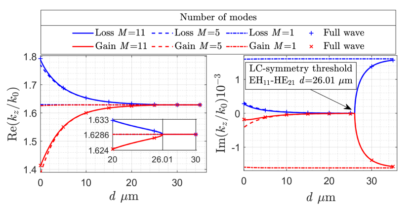
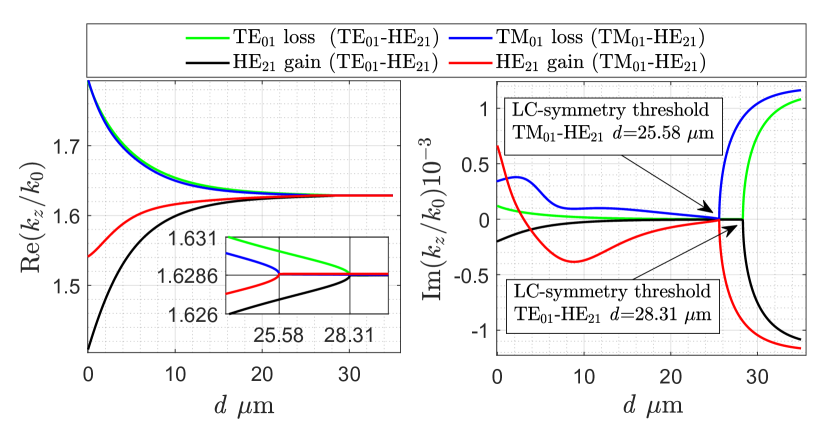
Figure 11: LC symmetry for the hybrid modes EH₁₁-HE₂₁ having different azimuthal indices.

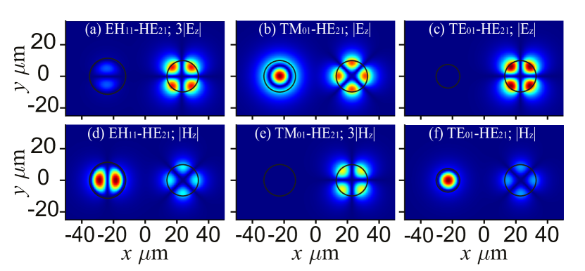
Figure 12: LC symmetry for the circularly symmetric TM₀₁, TE₀₁ and hybrid HE₂₁ modes.

Figure 13: (a), (b), (c) Electric field $|E_{z}|$ corresponding to the LC-symmetry thresholds of EH₁₁-HE₂₁, TM₀₁-HE₂₁ and TE₀₁-HE₂₁ mode pairs; (d), (e), (f) The corresponding magnetic field $|H_{z}|$.

As an example, let us consider the hybrid modes HE₂₁ and EH₁₁. For their dispersion curves to cross at $f=5.6$ THz and $k_{z}/k_{0}=1.6286$, the radii of the cylinders should be $R_{1}=11.44$ $\mu$m and $R_{2}=9.91$ $\mu$m. Figure 13 shows how the number of azimuthal harmonics in Eqs. (1)-(3) influences the possibility of the loss compensation phenomenon for these modes. In this figure, $M=2N+1$ is the number of terms took into account in the field sums. We see that the LC-symmetry threshold is observed for the values $\tan{\delta_{1}}=6.23\cdot 10^{-4}$ and $\tan{\delta_{2}}=-4.65\cdot 10^{-4}$ at the distance $d=26.01$ $\mu$m between the waveguides only for $M\geq 5$, i.e., the minimal set of harmonics includes the terms with $n=\{0,\pm 1,\pm 2\}$. This result is confirmed by the comparison with the independent full-wave calculation using COMSOL Multiphysics^® software (see symbols in Fig. 13). The required number of harmonics becomes larger for very close cylinders (near $d=0$) in order to save the consistency between the analytical and numerical methods as demonstrated with the calculations for $M=11$ in Fig. 13. Further, we omit the comparison with the full-wave simulations, since we are interested mainly in the region close to the LC-symmetry thresholds where the consistency is perfect even for relatively small $M$.

Since the hybrid modes can be coupled to the symmetric TM and TE modes, we analyze the loss compensation for such situations as well. For the pair TM₀₁-HE₂₁, for example, the LC-symmetry threshold can be reached at $d=25.58$ $\mu$m, whereas it is $d=28.31$ $\mu$m for TE₀₁-HE₂₁ (see Fig. 13). The parameters of the system should be taken as follows:

• TM₀₁-HE₂₁ – {$R_{1}=10$ $\mu$m, $R_{2}=9.91$ $\mu$m, $\epsilon_{r1}=\epsilon_{r2}=12$, $\tan{\delta_{1}}=5\cdot 10^{-4}$, $\tan{\delta_{2}}=-3.44\cdot 10^{-4}$};

• TE₀₁-HE₂₁ – {$R_{1}=7.48$ $\mu$m, $R_{2}=9.91$ $\mu$m, $\epsilon_{r1}=\epsilon_{r2}=12$, $\tan{\delta_{1}}=5\cdot 10^{-4}$, $\tan{\delta_{2}}=-3.32\cdot 10^{-4}$};

Note that for the TM₀₁-HE₂₁ pair at the LC-symmetry threshold, the longitudinal electric field $E_{z}$ is excited in both cylinders [Fig. 13(b)], whereas the longitudinal magnetic field $H_{z}$ exists only in the second one due to the HE₂₁ mode [Fig. 13(e)]. The opposite is true for the TE₀₁-HE₂₁ pair: $E_{z}$ is absent in the first cylinder [Fig. 13(c)], but $H_{z}$ is present in both waveguides [Fig. 13(f)].

V Conclusion

We employ the multi-mode analytical approach to study the $\mathcal{PT}$ and LC symmetries in the dielectric cylindrical waveguides with gain and loss. It is shown that for any predetermined frequency, one can realize the loss compensation by tuning the waveguides to the proper modes and to the proper radii. For the modes of either TM or TE nature, we can reach loss compensation either in the $\mathcal{PT}$-symmetric phase (when the waveguides have identical radii) or at the LC-symmetry threshold (when the waveguides are dissimilar). The loss compensation is also possible in the situations involving the hybrid modes with identical or different azimuthal indices. By tuning the waveguides radii, we obtained the LC-symmetry thresholds for a wide number of mode pairs, namely {HE-HE, HE-EH, HE-TM, HE-TE}. The results are illustrated with the profiles of $E_{z}$ and $H_{z}$ components of electromagnetic field at the corresponding EPs (LC- and $\mathcal{PT}$-symmetry thresholds) and corroborated by comparing with the full-wave simulations.

Our results show that the loss compensation phenomenon in loss-gain systems is the general effect taking place even in asymmetric systems, such as coupled dielectric waveguides of different radii. Tuning the waveguides to the desired modes simply by changing the distance between them and their radii allows to build the lossless system starting from the arbitrary values of gain and loss. These results significantly expand the understanding of the concepts of LC and $\mathcal{PT}$ symmetry and can be applied for the experimental implementation of new types of optical devices.

Appendix: Derivation of transverse field components

The transverse field components $(E_{r},H_{r},E_{\phi},H_{\phi})$ in all regions can be readily expressed in terms of axial components Eqs. (1)-(3) from the Maxwell equations. The $\phi$-components of the fields in the first cylinder (Region I) can be derived as:

$$\begin{split}E_{\phi}^{1}&=\frac{1}{k_{p,1}^{2}}\sum_{n}{\left[-\frac{k_{z}n}{r_{1}}A_{n}^{1}J_{n}(k_{p,1}r_{1})-i\omega\mu_{0}B_{n}^{1}k_{p,1}J^{\prime}_{n}(k_{p,1}r_{1})\right]e^{in\phi_{1}}},\\ H_{\phi}^{1}&=\frac{1}{k_{p,1}^{2}}\sum_{n}{\left[i\omega\epsilon_{1}k_{p,q}A_{n}^{1}J^{\prime}_{n}(k_{p,1}r_{1})-\frac{k_{z}n}{r_{1}}B_{n}^{1}J_{n}(k_{p,1}r_{1})\right]e^{in\phi_{1}}},\end{split}$$ (4)

The $\phi$-components of the fields inside the second cylinder (Region II):

$$\begin{split}E_{\phi}^{2}&=\frac{1}{k_{p,2}^{2}}\sum_{n}{\left[-\frac{k_{z}n}{r_{2}}A_{n}^{2}J_{n}(k_{p,2}r_{2})-i\omega\mu_{0}B_{n}^{2}k_{p,q}J^{\prime}_{n}(k_{p,2}r_{2})\right]e^{in\phi_{2}}},\\ H_{\phi}^{2}&=\frac{1}{k_{p,2}^{2}}\sum_{n}{\left[i\omega\epsilon_{2}k_{p,2}A_{n}^{2}J^{\prime}_{n}(k_{p,2}r_{2})-\frac{k_{z}n}{r_{2}}B_{n}^{2}J_{n}(k_{p,2}r_{2})\right]e^{in\phi_{2}}},\end{split}$$ (5)

For derivation of the fields in the Region III, we connect the coordinates $(r_{1},\phi_{1})$ and $(r_{2},\phi_{2})$ using the Graf addition theorem:

$$\begin{split}B_{n}(r_{1})e^{\pm in\phi_{1}}=\sum_{k=-N}^{N}{B_{n+k}(h)J_{k}(r_{2})e^{\mp ik\phi_{2}}}e^{\pm ik\pi},\\ B_{n}(r_{2})e^{\pm in\phi_{2}}=\sum_{k=-N}^{N}{B_{n+k}(h)J_{k}(r_{1})e^{\mp ik\phi_{1}}}e^{\pm in\pi},\end{split}$$ (6)

where $B_{n}(\cdot)$ is the $n$-th order cylindrical function and $h$ is the distance between the centers of two cylinders ($h=d+R_{1}+R_{2}$) (see Fig. 1). The $\phi$-components of the fields outside the cylinders in coordinates $(r_{1},\phi_{1})$ are:

$$\begin{split}E_{\phi}^{3}(r_{1},\phi_{1})=&\frac{1}{k_{p,3}^{2}}\sum_{n}\left\{-\frac{k_{z}n}{r_{1}}\left[C_{n}^{1}H_{n}^{(1,2)}(k_{p,3}r_{1})e^{in\phi_{1}}+\sum_{k}{C_{n}^{2}H_{n+k}^{(1,2)}(k_{p,3}h)J_{k}(k_{p,3}r_{1})e^{-ik\phi_{1}}e^{in\pi}}\right]-\right.\\ &\left.-i\omega\mu_{0}B_{n}^{2}k_{p,3}\left[D_{n}^{1}H_{n}^{{}^{\prime}(1,2)}(k_{p,3}r_{1})e^{in\phi_{1}}+\sum_{k}{D_{n}^{2}H_{n+k}^{(1,2)}(k_{p,3}h)J^{\prime}_{k}(k_{p,3}r_{1})e^{-ik\phi_{1}}e^{in\pi}}\right]\right\},\\ H_{\phi}^{3}(r_{1},\phi_{1})=&\frac{1}{k_{p,3}^{2}}\sum_{n}\left\{i\omega\epsilon_{3}k_{p,3}\left[C_{n}^{1}H_{n}^{{}^{\prime}(1,2)}(k_{p,3}r_{1})e^{in\phi_{1}}+\sum_{k}{C_{n}^{2}H_{n+k}^{(1,2)}(k_{p,3}h)J^{\prime}_{k}(k_{p,3}r_{1})e^{-ik\phi_{1}}e^{in\pi}}\right]\right.-\\ &-\left.\frac{k_{z}n}{r_{1}}\left[D_{n}^{1}H_{n}^{(1,2)}(k_{p,3}r_{1})e^{in\phi_{1}}+\sum_{k}{D_{n}^{2}H_{n+k}^{(1,2)}(k_{p,3}h)J_{k}(k_{p,3}r_{1})e^{-ik\phi_{1}}e^{in\pi}}\right]\right\},\end{split}$$ (7)

The $\phi$-components of the fields in the Region III in the coordinates $(r_{2},\phi_{2})$ are:

$$\begin{split}E_{\phi}^{3}(r_{2},\phi_{2})=&\frac{1}{k_{p,3}^{2}}\sum_{n}\left\{-\frac{k_{z}n}{r_{2}}\left[\sum_{k}{C_{n}^{1}H_{n+k}^{(1,2)}(k_{p,3}h)J_{k}(k_{p,3}r_{2})e^{ik(\pi-\phi_{2})}}+C_{n}^{2}H_{n}^{(1,2)}(k_{p,3}r_{2})e^{in\phi_{2}}\right]-\right.\\ &\left.-i\omega\mu_{0}k_{p,3}\left[\sum_{k}{D_{n}^{1}H_{n+k}^{(1,2)}(k_{p,3}h)J^{\prime}_{k}(k_{p,3}r_{2})e^{ik(\pi-\phi_{2})}}+D_{n}^{2}H_{n}^{{}^{\prime}(1,2)}(k_{p,3}r_{2})e^{in\phi_{2}}\right]\right\},\\ H_{\phi}^{3}(r_{2},\phi_{2})=&\frac{1}{k_{p,3}^{2}}\sum_{n}\left\{i\omega\epsilon_{3}k_{p,3}\left[\sum_{k}{C_{n}^{1}H_{n+k}^{(1,2)}(k_{p,3}h)J^{\prime}_{k}(k_{p,3}r_{2})e^{ik(\pi-\phi_{2})}}+C_{n}^{2}H_{n}^{{}^{\prime}(1,2)}(k_{p,3}r_{2})e^{in\phi_{2}}\right]\right.-\\ &-\left.\frac{k_{z}n}{r_{2}}\left[\sum_{k}{D_{n}^{1}H_{n+k}^{(1,2)}(k_{p,3}h)J_{k}(k_{p,3}r_{2})e^{ik(\pi-\phi_{2})}}+D_{n}^{2}H_{n}^{(1,2)}(k_{p,3}r_{2})e^{in\phi_{2}}\right]\right\},\end{split}$$ (8)

The explicit form of the dispersion relation is the condition of zero determinant of the following system of equations:

$$\begin{split}\tilde{A}_{m}^{1}J_{m}(k_{p,1}r_{1})=\tilde{C}_{m}^{1}H_{m}^{(1,2)}(k_{p,3}r_{1})+\sum_{n}{\tilde{C}_{n}^{2}H_{m-n}^{(1,2)}(k_{p,3}h)J_{m}(k_{p,3}r_{1})},\\ B_{m}^{1}J_{m}(k_{p,1}r_{1})=D_{m}^{1}H_{m}^{(1,2)}(k_{p,3}r_{1})+\sum_{n}{D_{n}^{2}H_{m-n}^{(1,2)}(k_{p,3}h)J_{m}(k_{p,3}r_{1})},\\ \tilde{A}_{m}^{2}J_{m}(k_{p,2}r_{2})=\sum_{n}{\tilde{C}_{n}^{1}H_{m-n}^{(1,2)}(k_{p,3}h)J_{m}(k_{p,3}r_{2})}+\tilde{C}_{m}^{2}H_{m}^{(1,2)}(k_{p,3}r_{2}),\\ B_{m}^{2}J_{m}(k_{p,2}r_{2})=\sum_{n}{D_{n}^{1}H_{m-n}^{(1,2)}(k_{p,3}h)J_{m}(k_{p,3}r_{2})}+D_{m}^{2}H_{m}^{(1,2)}(k_{p,3}r_{2}),\\ \frac{1}{k_{p,1}^{2}}\left[-\frac{k_{z}m}{r_{1}}\tilde{A}_{m}^{1}J_{m}(k_{p,1}r_{1})-ik_{0}B_{m}^{1}k_{p,1}J^{\prime}_{m}(k_{p,1}r_{1})\right]=\\ =\frac{1}{k_{p,3}^{2}}\left\{-\frac{k_{z}m}{r_{1}}\left[\tilde{C}_{m}^{1}H_{m}^{(1,2)}(k_{p,3}r_{1})+\sum_{n}{\tilde{C}_{n}^{2}H_{m-n}^{(1,2)}(k_{p,3}h)J_{m}(k_{p,3}r_{1})}\right]\right.-\\ -\left.ik_{0}k_{p,3}\left[D_{m}^{1}H_{m}^{{}^{\prime}(1,2)}(k_{p,3}r_{1})+\sum_{n}{D_{n}^{2}}H_{m-n}^{(1,2)}(k_{p,3}h)J^{\prime}_{m}(k_{p,3}r_{1})\right]\right\},\\ \frac{1}{k_{p,1}^{2}}\left[ik_{0}\epsilon_{1}k_{p,1}\tilde{A}_{m}^{1}J^{\prime}_{m}(k_{p,1}r_{1})-\frac{k_{z}m}{r_{1}}B_{m}^{1}J_{m}(k_{p,1}r_{1})\right]=\\ =\frac{1}{k_{p,3}^{2}}\left\{ik_{0}\epsilon_{3}k_{p,3}\left[\tilde{C}_{m}^{1}H_{m}^{{}^{\prime}(1,2)}(k_{p,3}r_{1})+\sum_{n}{\tilde{C}_{n}^{2}H_{m-n}^{(1,2)}(k_{p,3}h)J^{\prime}_{m}(k_{p,3}r_{1})}\right]\right.-\\ -\left.\frac{k_{z}m}{r_{1}}\left[D_{m}^{1}H_{m}^{(1,2)}(k_{p,3}r_{1})+\sum_{n}{D_{n}^{2}}H_{m-n}^{(1,2)}(k_{p,3}h)J_{m}(k_{p,3}r_{1})\right]\right\},\\ \frac{1}{k_{p,2}^{2}}\left[-\frac{k_{z}m}{r_{2}}\tilde{A}_{m}^{2}J_{m}(k_{p,2}r_{2})-ik_{0}B_{m}^{2}k_{p,2}J^{\prime}_{m}(k_{p,2}r_{2})\right]=\\ =\frac{1}{k_{p,3}^{2}}\left\{-\frac{k_{z}m}{r_{2}}\left[\sum_{n}{\tilde{C}_{n}^{1}H_{m-n}^{(1,2)}(k_{p,3}h)J_{m}(k_{p,3}r_{2})}+\tilde{C}_{m}^{2}H_{m}^{(1,2)}(k_{p,3}r_{2})\right]\right.-\\ -\left.ik_{0}k_{p,3}\left[\sum_{n}{D_{n}^{1}}H_{m-n}^{(1,2)}(k_{p,3}h)J^{\prime}_{m}(k_{p,3}r_{2})+D_{m}^{2}H_{m}^{{}^{\prime}(1,2)}(k_{p,3}r_{2})\right]\right\},\\ \frac{1}{k_{p,2}^{2}}\left[ik_{0}\epsilon_{2}k_{p,2}\tilde{A}_{m}^{2}J^{\prime}_{m}(k_{p,2}r_{2})-\frac{k_{z}m}{r_{2}}B_{m}^{2}J_{m}(k_{p,2}r_{2})\right]=\\ =\frac{1}{k_{p,3}^{2}}\left\{ik_{0}\epsilon_{3}k_{p,3}\left[\sum_{n}{\tilde{C}_{n}^{1}H_{m-n}^{(1,2)}(k_{p,3}h)J^{\prime}_{m}(k_{p,3}r_{2})}+\tilde{C}_{m}^{2}H_{m}^{{}^{\prime}(1,2)}(k_{p,3}r_{2})\right]\right.-\\ -\left.\frac{k_{z}m}{r_{2}}\left[\sum_{n}{D_{n}^{1}}H_{m-n}^{(1,2)}(k_{p,3}h)J_{m}(k_{p,3}r_{2})+D_{m}^{2}H_{m}^{(1,2)}(k_{p,3}r_{2})\right]\right\}.\end{split}$$ (9)

Here $\tilde{A}_{n}^{1,2}=\sqrt{\epsilon_{0}/\mu_{0}}A_{n}^{1,2}$, $\tilde{C}_{n}^{1,2}=\sqrt{\epsilon_{0}/\mu_{0}}C_{n}^{1,2}$.

References

- Zyablovsky et al. [2014] A. A. Zyablovsky, A. P. Vinogradov, A. A. Pukhov, A. V. Dorofeenko, and A. A. Lisyansky, PT-symmetry in optics, Phys. Usp. 57, 1063 (2014).
- Feng et al. [2017] L. Feng, R. El-Ganainy, and L. Ge, Non-Hermitian photonics based on parity–time symmetry, Nat. Photon. 11, 752 (2017).
- El-Ganainy et al. [2018] R. El-Ganainy, K. G. Makris, M. Khajavikhan, Z. H. Musslimani, S. Rotter, and D. N. Christodoulides, Non-Hermitian physics and PT symmetry, Nat. Phys. 14, 11 (2018).
- Bender and Boettcher [1998] C. M. Bender and S. Boettcher, Real spectra in non-Hermitian hamiltonians having PT symmetry, Phys. Rev. Lett. 80, 5243 (1998).
- Makris et al. [2008] K. G. Makris, R. El-Ganainy, D. N. Christodoulides, and Z. H. Musslimani, Beam dynamics in PT symmetric optical lattices, Phys. Rev. Lett. 100, 103904 (2008).
- Rüter et al. [2010] C. E. Rüter, K. G. Makris, R. El-Ganainy, D. N. Christodoulides, M. Segev, and D. Kip, Observation of parity–time symmetry in optics, Nat. Phys. 6, 192 (2010).
- Schindler et al. [2011] J. Schindler, A. Li, M. C. Zheng, F. M. Ellis, and T. Kottos, Experimental study of active lrc circuits with symmetries, Phys. Rev. A 84, 040101 (2011).
- Zhu et al. [2014] X. Zhu, H. Ramezani, C. Shi, J. Zhu, and X. Zhang, -symmetric acoustics, Phys. Rev. X 4, 031042 (2014).
- Chitsazi et al. [2017] M. Chitsazi, H. Li, F. M. Ellis, and T. Kottos, Experimental realization of floquet -symmetric systems, Phys. Rev. Lett. 119, 093901 (2017).
- Hess et al. [2012] O. Hess, J. B. Pendry, S. A. Maier, R. F. Oulton, J. M. Hamm, and K. L. Tsakmakidis, Active nanoplasmonic metamaterials, Nat. Mater. 11, 573 (2012).
- Krasnok and Alù [2020] A. Krasnok and A. Alù, Active nanophotonics, Proceedings of the IEEE 108, 628 (2020).
- Novitsky et al. [2017] D. V. Novitsky, V. R. Tuz, S. L. Prosvirnin, A. V. Lavrinenko, and A. V. Novitsky, Transmission enhancement in loss-gain multilayers by resonant suppression of reflection, Phys. Rev. B 96, 235129 (2017).
- Özdemir et al. [2019] Ş. K. Özdemir, S. Rotter, F. Nori, and L. Yang, Parity-time symmetry and exceptional points in photonics, Nat. Mater. 18, 783 (2019).
- Miri and Alù [2019] M.-A. Miri and A. Alù, Exceptional points in optics and photonics, Science 363, 10.1126/science.aar7709 (2019).
- Ding et al. [2016] K. Ding, G. Ma, M. Xiao, Z. Q. Zhang, and C. T. Chan, Emergence, coalescence, and topological properties of multiple exceptional points and their experimental realization, Phys. Rev. X 6, 021007 (2016).
- Jiang and Xiang [2020] T. Jiang and Y. Xiang, Perfectly-matched-layer method for optical modes in dielectric cavities, Phys. Rev. A 102, 053704 (2020).
- Wang et al. [2020] X.-Y. Wang, F.-F. Wang, and X.-Y. Hu, Waveguide-induced coalescence of exceptional points, Phys. Rev. A 101, 053820 (2020).
- Gomis-Bresco et al. [2019] J. Gomis-Bresco, D. Artigas, and L. Torner, Transition from Dirac points to exceptional points in anisotropic waveguides, Phys. Rev. Research 1, 033010 (2019).
- Abdrabou and Lu [2019] A. Abdrabou and Y. Y. Lu, Exceptional points for resonant states on parallel circular dielectric cylinders, J. Opt. Soc. Am. B 36, 1659 (2019).
- Chen et al. [2017] W. Chen, Ş. K. Özdemir, G. Zhao, J. Wiersig, and L. Yang, Exceptional points enhance sensing in an optical microcavity, Nature 548, 192 (2017).
- Hodaei et al. [2017] H. Hodaei, A. U. Hassan, S. Wittek, H. Garcia-Gracia, R. El-Ganainy, D. N. Christodoulides, and M. Khajavikhan, Enhanced sensitivity at higher-order exceptional points, Nature 548, 187 (2017).
- Feng et al. [2014] L. Feng, Z. J. Wong, R.-M. Ma, Y. Wang, and X. Zhang, Single-mode laser by parity-time symmetry breaking, Science 346, 972 (2014).
- Hodaei et al. [2014] H. Hodaei, M.-A. Miri, M. Heinrich, D. N. Christodoulides, and M. Khajavikhan, Parity-time–symmetric microring lasers, Science 346, 975 (2014).
- Hokmabadi et al. [2019] M. P. Hokmabadi, A. Schumer, D. N. Christodoulides, and M. Khajavikhan, Non-Hermitian ring laser gyroscopes with enhanced Sagnac sensitivity, Nature 576, 70 (2019).
- Lai et al. [2019] Y.-H. Lai, Y.-K. Lu, M.-G. Suh, Z. Yuan, and K. Vahala, Observation of the exceptional-point-enhanced Sagnac effect, Nature 576, 65 (2019).
- Longhi [2010] S. Longhi, -symmetric laser absorber, Phys. Rev. A 82, 031801 (2010).
- Wong et al. [2016] Z. J. Wong, Y.-L. Xu, J. Kim, K. O’Brien, Y. Wang, L. Feng, and X. Zhang, Lasing and anti-lasing in a single cavity, Nat. Photon. 10, 796 (2016).
- Novitsky et al. [2018] D. V. Novitsky, A. Karabchevsky, A. V. Lavrinenko, A. S. Shalin, and A. V. Novitsky, symmetry breaking in multilayers with resonant loss and gain locks light propagation direction, Phys. Rev. B 98, 125102 (2018).
- Doppler et al. [2016] J. Doppler, A. A. Mailybaev, J. Böhm, U. Kuhl, A. Girschik, F. Libisch, T. J. Milburn, P. Rabl, N. Moiseyev, and S. Rotter, Dynamically encircling an exceptional point for asymmetric mode switching, Nature 537, 76 (2016).
- Liu et al. [2020] Q. Liu, S. Li, B. Wang, S. Ke, C. Qin, K. Wang, W. Liu, D. Gao, P. Berini, and P. Lu, Efficient mode transfer on a compact silicon chip by encircling moving exceptional points, Phys. Rev. Lett. 124, 153903 (2020).
- Hassan et al. [2017] A. U. Hassan, B. Zhen, M. Soljačić, M. Khajavikhan, and D. N. Christodoulides, Dynamically encircling exceptional points: Exact evolution and polarization state conversion, Phys. Rev. Lett. 118, 093002 (2017).
- Wang et al. [2019] S. Wang, B. Hou, W. Lu, Y. Chen, Z. Q. Zhang, and C. T. Chan, Arbitrary order exceptional point induced by photonic spin–orbit interaction in coupled resonators, Nat. Commun. 10, 832 (2019).
- Zhong et al. [2020] Q. Zhong, J. Kou, Ş K.. Özdemir, and R. El-Ganainy, Hierarchical construction of higher-order exceptional points, Phys. Rev. Lett. 125, 203602 (2020).
- Ryu et al. [2019] J. Ryu, S. Gwak, J. Kim, H.-H. Yu, J.-H. Kim, J.-W. Lee, C.-H. Yi, and C.-M. Kim, Hybridization of different types of exceptional points, Photon. Res. 7, 1473 (2019).
- Zhang and Chan [2019] X.-L. Zhang and C. T. Chan, Dynamically encircling exceptional points in a three-mode waveguide system, Comm. Phys. 2, 63 (2019).
- Huang [1994] W.-P. Huang, Coupled-mode theory for optical waveguides: an overview, J. Opt. Soc. Am. A 11, 963 (1994).
- Dai et al. [2012] D. Dai, Y. Tang, and J. E. Bowers, Mode conversion in tapered submicron silicon ridge optical waveguides, Opt. Express 20, 13425 (2012).
- Zhang et al. [2015] Z. Zhang, X. Hu, and J. Wang, On-chip optical mode exchange using tapered directional coupler, Sci. Rep. 5, 16072 (2015).
- Kim et al. [2017] S. Kim, K. Han, C. Wang, J. A. Jaramillo-Villegas, X. Xue, C. Bao, Y. Xuan, D. E. Leaird, A. M. Weiner, and M. Qi, Dispersion engineering and frequency comb generation in thin silicon nitride concentric microresonators, Nat. Commun. 8, 372 (2017).
- Klimov et al. [2018] V. V. Klimov, I. V. Zabkov, D. V. Guzatov, and A. P. Vinogradov, Loss compensation symmetry in dimers made of gain and lossy nanoparticles, Laser Phys. Lett. 15, 035901 (2018).
- Hlushchenko et al. [2020] A. V. Hlushchenko, V. I. Shcherbinin, D. V. Novitsky, and V. R. Tuz, Loss compensation symmetry in a multimode waveguide coupler, Laser Phys. Lett. 17, 116202 (2020).
- White et al. [2002] T. P. White, B. T. Kuhlmey, R. C. McPhedran, D. Maystre, G. Renversez, C. Martijn de Sterke, and L. C. Botten, Multipole method for microstructured optical fibers. I. Formulation, J. Opt. Soc. Am. B 19, 2322 (2002).
- Kominis et al. [2016] Y. Kominis, T. Bountis, and S. Flach, The asymmetric active coupler: Stable nonlinear supermodes and directed transport, Sci. Rep. 6, 33699 (2016).
- Kominis et al. [2017] Y. Kominis, T. Bountis, and S. Flach, Stability through asymmetry: Modulationally stable nonlinear supermodes of asymmetric non-hermitian optical couplers, Phys. Rev. A 95, 063832 (2017).
- Lamb [1996] J. W. Lamb, Miscellaneous data on materials for millimetre and submillimetre optics, Int. J. Infrared Millimeter Waves 17, 1997–2034 (1996).