Identification of high-energy astrophysical point sources via hierarchical Bayesian nonparametric clustering
Address for correspondence: sottosanti@stat.unipd.it)
Abstract
The light we receive from distant astrophysical objects carries information about their origins and the physical mechanisms that power them. The study of these signals, however, is complicated by the fact that observations are often a mixture of the light emitted by multiple localized sources situated in a spatially-varying background. A general algorithm to achieve robust and accurate source identification in this case remains an open question in astrophysics.
This paper focuses on high-energy light (such as X-rays and -rays), for which observatories can detect individual photons (quanta of light), measuring their incoming direction, arrival time, and energy. Our proposed Bayesian methodology uses both the spatial and energy information to identify point sources, that is, separate them from the spatially-varying background, to estimate their number, and to compute the posterior probabilities that each photon originated from each identified source. This is accomplished via a Dirichlet process mixture while the background is simultaneously reconstructed via a flexible Bayesian nonparametric model based on B-splines. Our proposed method is validated with a suite of simulation studies and illustrated with an application to a complex region of the sky observed by the Fermi Gamma-ray Space Telescope.
1 Introduction
Astronomy aims to extend our knowledge of the physical processes that underlie the wide variety of phenomena that exist in the Universe. Electromagnetic radiation, that is, light, is the primary carrier of astronomical information from the Universe to us. The nature of cosmic objects is imprinted in the light that they emit and that we subsequently detect. However, photons (that is, quanta of light) do not bear labels telling us what object they originated from. In fact, when it reaches Earth, light is characterized by only 6 numbers: its time of arrival and energy (measured in eV111An eV (electronvolt) is a unit of energy commonly used in particle physics. It gives the kinetic energy acquired by an electron when accelerated from rest across a potential difference of 1 volt. The symbol GeV denotes an energy of eV.), and its two dimensional directions of provenance and polarization (a unit vector perpendicular to the direction of travel indicating the oscillation plane of the electromagnetic wave). This article focuses on high-energy light (e.g., X-rays and -rays), where we may hope to measure a subset of these properties for individually detected photons. At lower energies (e.g., optical, infrared, radio waves), photon properties are averaged over an area of the sky. In both cases, the resulting astronomical dataset is generally the realization of a mixture model in which light generated by multiple sources is blended together in a single image or collection of detected photons.
The light received from a region of the sky is the result of the superposition of different physical sources. A basic distinction, and an important one for astronomers, is between localized and diffuse sources: localized sources are those whose angular size, as viewed from the Earth, is much smaller than the angular resolution of the detector. A localized source appears as a sharply defined region of high intensity. The prototypical example is a star, which nearly always appears as a so-called “point source” in an astronomical image. In contrast, diffuse sources appear as extended regions of variable intensity across a portion of the sky. An important example in -ray astronomy are the clouds of gas in the Milky Way, which emit -ray photons as cosmic rays collide with the hydrogen and helium that make up the clouds.
The necessary first step in many physics analyses is the the identification of distinct astrophysical sources — a procedure called “source extraction”. The goal of source extraction is to detect new astronomical objects and infer basic properties such as their location and the energy distribution of the light they emit. Once sources are identified, they can be further studied by restricting the analysis to the region or collection of photons that are attributed to them. Conversely, separating point sources from a diffuse background is essential to study the physical processes which give rise to the diffuse background itself.
From a statistical perspective, identifying a source means quantifying the evidence of its presence in an observed region of the sky and placing constraints on its location and properties. In X-ray and -ray astronomy, the data consist of an event list giving the measured sky coordinates, energy, and arrival time of each photon detected by the instrument. The distribution of the sky coordinates of the events forms an image and the distribution of energies forms a spectrum.
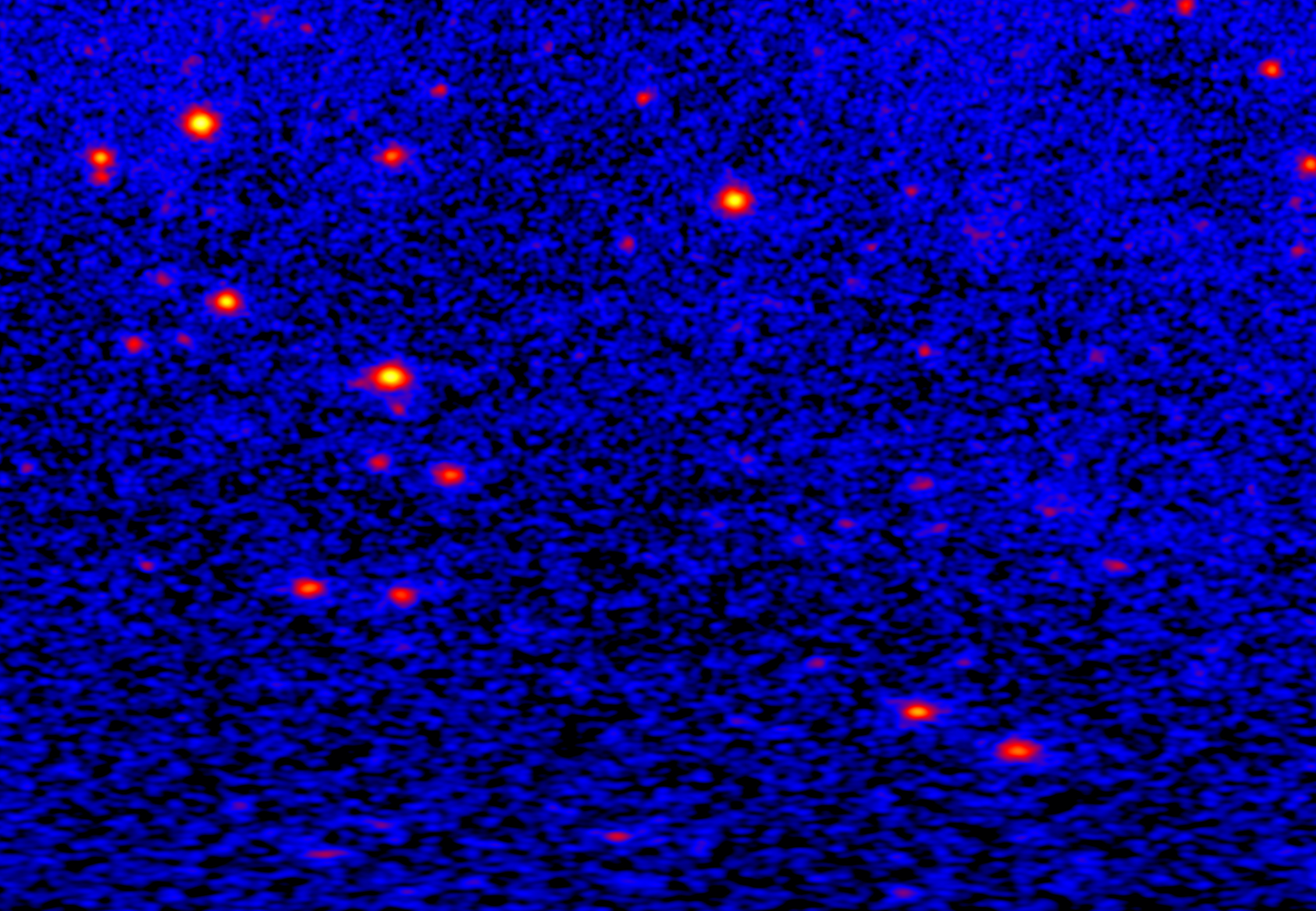
Identifying point sources is challenging for several reasons: the sky coordinates are noisy estimates, interesting sources may be faint and emit only a few photons, and point sources are embedded in a diffuse background, generally a significant component of the data. The intensity of the background and measurement error in the recorded sky coordinates of the photons both vary with location and energy, that is, across the joint domain of the image and the spectrum. Directions in the sky near the Galactic plane, for example, have a high level of emission from diffuse gas clouds, whereas emission at high Galactic latitudes is dominated by a more or less isotropic -ray background component due to the integrated emission of all the faint sources along each line of sight through the Universe, as shown in Figure 1. The process of source extraction is generally easier in the latter region where the background can be more simply modeled as a spatially uniform process.
1.1 Astrophysical source extraction
Source extraction has attracted a growing interest both in the astronomical and the statistical literature. In the last twenty years, new technologies have massively increased the precision of detectors and the size of the data sets they generate. Astronomical images now contain multitudes of localized sources over vast regions of the sky. Previously manual or ad hoc analyses are now impractical and introduce uncontrolled biases into the statistical characterization of populations of sources. The resulting rich new data resources pose significant statistical challenges and have stimulated the development of new statistical techniques and advanced computational methods.
Hobson et al. (2010) differentiate methods according to whether they are designed to extract a single source or multiple sources simultaneously. While the former subject has received considerable attention since the early 1990s (Kraft et al., 1991; Mattox et al., 1996; van Dyk et al., 2001; Protassov et al., 2002; Park et al., 2006; Weisskopf et al., 2007; Knoetig, 2014), the latter has attracted a growing interest only recently, partially because of its higher computational cost. For example, see Savage and Oliver, (2007), Guglielmetti et al. (2009), Primini and Kashyap (2014) and Jones et al. (2015) for X-ray data and Acero et al. (2015) and Selig et al. (2015) for -ray data. Simultaneous multiple source extraction is preferable over single-source extraction in cases where sources overlap spatially in images, a case in which single-source extraction would yield misleading results.
All source extraction methods must account for the presence of a diffuse background emission in the data. When the background is low or relatively constant over the region of interest, its spatial and energy components can be modelled as uniform (e.g. Jones et al., 2015; Meyer et al., 2021); alternatively, one can consider the Bayesian aperture-photometry approach of Primini and Kashyap (2014) for low-counts images. However, for multiple sources extraction methods the modeling of the background is more challenging, since the intensity of the background can vary across the region of interest, as shown in Figure 1. For example, Guglielmetti et al. (2009) use a Poisson-based mixture model with thin-plate splines for the background of X-ray count images with intense and prominent background contamination.
In contrast to the data-driven methods above, an alternative approach is to adopt a physics-based model for the diffuse background emission. For instance, Acero et al. (2016) define a physical model of the Milky Way based on approximate knowledge of the distribution of gas in the Galactic disk, the locations and properties of sources of cosmic rays, dust maps, etc. Combined with physics models for cosmic ray diffusion and high-energy particle physics, they generate “templates” for the approximate -ray emission expected from various components. A final background model is then found by fitting these templates to the full-sky -ray data collected by the Fermi Large Area Telescope (LAT). The method has been widely used to analyse the data collected by the Fermi LAT to build detailed catalogues of sources, the latest of which is presented in Abdollahi et al., (2020). Additionally, the physics-based templates can be used, for example, in conjunction with the method of Stein et al. (2015) to detect unknown structures added to a known image (e.g., a known background). Nonetheless, because the physics model is incomplete, the resulting templates are statistically inconsistent with the observed all-sky data and residuals between model and data are incorporated into the background model according to an ad hoc procedure. Therefore, the Fermi model may inadvertently subsume some point sources into its background estimate, masking their signal in subsequent analyses. In addition, this tool provides only a point estimate of the background morphology, without any measure of uncertainty.
As a completely data-driven approach to characterize the diffuse background in photon observations, Selig and Enßlin (2015) propose their own empirical background reconstruction based on Information Field Theory, an alternative approach to the one of Acero et al. (2016). This tool is exploited by Selig et al. (2015) to analyse the Fermi LAT sky. The most recent background fit of the Galactic center in -rays, provided by Abazajian et al., (2020), shows that a proper treatment of the Fermi LAT data at their highest energies is fundamental to improve the understanding of the diffuse background component. The resulting inferences on physical process of interest (for example, the presence of a diffuse emission due to dark matter) can strongly depend on the accuracy of the source extraction procedure. Most available simultaneous sources extraction methods require specification of the number of sources in advance (Savage and Oliver,, 2007; Ray et al., 2011) or are computationally limited to a maximum number of sources detectable (Primini and Kashyap, 2014). An alternative approach, which also does not require the specification of the number of sources in advance, but only applies to spatially well-separated sources, is Feroz and Hobson, (2008). This is a nested sampling method which exploits Bayesian model comparison to detect and characterise multiple modes in the marginal distribution of the data. The recent work of Jones et al. (2015), which inspired this paper, considers a Bayesian extraction method based on a finite mixture model where the number of sources is inferred; see also Daylan et al., (2017). Computationally, the model is fit using reversible-jump Markov chain Monte Carlo (MCMC) (Richardson and Green,, 1997).
1.2 Main goals and outline
In this work we propose a novel, fully data-driven approach to simultaneously extract the signal of high-energy point sources and reconstruct the diffuse background emission that extends over a region of the sky. The method exploits both the spatial coordinates and the energy of the photons to probabilistically allocate them to sources. These probabilities can then be used in secondary analyses in place of an absolute classification. We utilize Bayesian nonparametric modelling to overcome the limitations of the existent approaches to locating sources in a map that is highly contaminated by background. In particular, our proposed method: i) automatically determines the unknown number of point sources in the map; ii) probabilistically clusters the photons into these sources according to their sky coordinates and energy; and iii) flexibly estimates the underlying intensity of the background emission without relying on either a previous physical understanding or empirical reconstructions of the background map.
Our approach exploits the advantages of mixture modelling and extends the model of Jones et al. (2015) by using an infinite mixture induced by a Dirichlet process (DP) prior (Ferguson, 1973). In addition, we use Gibbs sampling algorithms for Bayesian nonparametric methods (Müller et al., 2015) which deliver better scaling properties with the mixture size than Green’s reversible-jump MCMC, thus providing practical advantages in model fitting. Along with source extraction, our method simultaneously reconstructs the background using a flexible model – a central advantage, as a poor background choice may lead to misleading results such as the identification of spurious sources, or the incorrect absorption of sources into the background. Jones et al. (2015) employ a uniform model both for the background map and spectrum. However, this assumption is inappropriate for heavily contaminated regions such as those close to the Galactic plane. Costantin et al., (2020) extend the model of Jones et al. (2015) using a bivariate exponential distribution for the background map. However, their method is designed for the analysis of a particular field and cannot be directly applied more generally. Additionally, their method does not account for irregularities in the background and thus may result in a large number of false detections. Our innovative solution is to model the background component by combining Bayesian nonparametric techniques with B-splines to fully reconstruct the background morphology over the map. Previous comparable approaches (Denison et al., 1998; Biller, 2000; DiMatteo et al., 2001; Sharef et al., 2010) adopt reversible-jump MCMC to select the active spline functions. Other competitive models based on splines require solving minimization problems, which in practice might be unfeasible (Guglielmetti et al., 2009; Schellhase and Kauermann, 2012). By contrast, we adopt faster Gibbs sampling algorithms for fitting our Bayesian nonparametric model.
This paper is structured in six sections. Section 2 presents our novel Bayesian nonparametric mixture model for signal extraction with high background contamination, first addressing spatial data only, that is, ignoring energy, and then extended to jointly model spatial data and spectra. Section 3 recasts the model as a mixture of DP mixtures and presents our Gibbs sampler. The model is validated in Section 4 with a suite of simulation studies, first illustrating the method and then demonstrating the advantage of including spectral data. An application to a region of the sky using Fermi LAT data is presented in Section 5 and discussion appears in Section 6. Technical details of the Gibbs sampling algorithm are presented in Appendix A, and additional results related to our simulation studies appear in Appendix B.
2 The statistical model
Let index a collection of photons (that is, events) with sky coordinates and energy .
2.1 The spatial model
As each event may originate either from a point source or from background, we formalize a mixture model for the sky coordinates,
| (1) |
where and are the unknown density functions for the sky coordinates of source events and background events, with parameters and , respectively. Finally, is a mixing parameter, which follows a distribution, where is a known hyperparameter. We collect the unknown parameters in .
2.2 The spatial source model
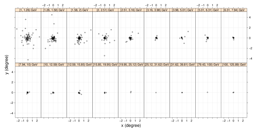
We begin with a model for the recorded sky coordinates of photons from source , with location . Although we only consider point-like sources, due to measurement noise the observed sky coordinates form a distribution around the true source location. This distribution is called the Point Spread Function (PSF). The shape of the PSF varies with photon energy: qualitatively, the Fermi LAT instrument measures more accurately the arrival direction of high-energy photons (i.e., in this case the PSF concentrates more tightly around the true source location), while the PSF of low-energy photons has a larger spread. Additionally, high-energy photons are generically rarer than low-energy photons, as the flux from astrophysical sources generally follows a negative power law with energy (sometimes with exponential cut-offs past a certain energy threshold, though the details are unimportant here). The Fermi LAT PSF (Ackermann et al., 2012) is tabulated so that gives the probability that a photon with energy and true sky coordinates is recorded in the instrumental pixel containing . Here, the instrumental pixel is the smallest addressable unit, measured in degrees, into which the area of the whole sky map is subdivided. Figure 2 uses simulated data to illustrate how the distribution of the recorded sky coordinates for a point source observed with the Fermi LAT varies with photon energy.
Formulating a model based on the PSF for multiple sources requires care because (a) the total number of sources is unknown, (b) the sources have different intensities, and (c) no a priori information on the sources’ locations is available. To address these issues, we propose the following model:
| (2) |
where is a DP prior with concentration parameter and base measure . Model (2) is known as a DP mixture and formulates by mixing the kernel PSF with respect to the unknown measure . is the prior distribution for and is assumed to be uniform over the map . (For a review of Bayesian nonparametrics, see Müller et al. (2015)).
2.3 The spatial background model
In (1), in the density of background photons across the image. As mentioned in Section 1, high-energy astrophysics images can be heavily contaminated by a non-uniform background (both in spatial location and energy). Because the background is the result of several astronomical phenomena that cannot be predicted from first principles, no analytical distribution is available. We therefore propose a flexible nonparametric solution based on B-splines.
The B-spline basis function of order is defined on a vector of knots ,
| (3) |
where is the vector with element removed. Starting from , a basis of order is defined recursively from the bases of smaller orders. By construction, (3) is always positive between and and zero elsewhere. Although is unimodal for , it can assume many different shapes depending on the location of the knots and can be normalised to the density function ; see de Boor (2001) for a full review. We define the bivariate density
where and denote the knots of the longitude and of the latitude B-splines, respectively; thus, and , for . Here we use splines of order 4 as they ensure sufficient flexibility without requiring too many knots. We then model the background as
| (4) |
This is an infinite mixture of normalised B-spline functions induced by a DP prior, but in practice a sample of photons from the background leads to a finite mixture with at most components. The base measure, , is the prior distribution for the sets of longitude and latitude knots. The ordering of the knots is maintained by assuming the middle knot is uniformly distributed over the limits of the map, e.g., , and that the remaining knots are conditionally uniformly distributed over their appropriate ranges. Specifically, given , we assume and ; given , we assume and given we assume ; likewise for , but replacing and with and .
2.4 The joint spatial-spectral model
We wish to extend Model (1) to jointly model both the sky coordinates and energies of the photons. Astrophysical sources typically have power-law spectra (e.g., Acero et al., 2015), where the number of emitted photons decreases with energy according to , where . Therefore, we propose Pareto distributions for both the source and background energies, that is,
| (5) | ||||
where and is a Pareto density with shape parameter , scale parameter , and support ; we set , the lower limit of the instrumental energy range. We specify and to exploit the conjugacy between the Gamma and the Pareto distributions.
Equation (5) ignores two effects. First, not all photons that arrive at the telescope from a fixed direction are detected with the same probability. Very often this detection probability depends on energy and is quantified by the effective area of the detector (which is a function of energy). Second, as with direction , photon energies are measured with uncertainty. Ideally, in (5) should be replaced with
| (6) |
where is the true photon energy, is the intrinsic energy spectrum of the source or background component, is the exposure (effective area integrated over the observation time), and is the probability density function of the observed energy given the true energy. This is straightforward to implement but introduces a performance penalty. In our application to the Fermi LAT in Sections 4 and 5, we use an energy range where the effective area is approximately constant and in which the energy uncertainty is relatively small, around 10%. Thus, the approximation implicit in (5) is a good one. Alternatively, (5) can be interpreted as modelling the observed energy spectrum, rather than the true spectrum, as a power-law. The parameter then potentially loses its physical meaning. However, for broad energy ranges, small energy uncertainty, and intrinsic power-law spectra, the observed power-law index equals the intrinsic index.
Model (5) specifies a common Pareto distribution for the spectra of all the sources. In practice, however, we expect the source spectra to differ. As we illustrate in Section 4.3, even with this simplifying assumption, the Joint Spatial-Spectral Model defined in Formula (5) out-performs the Spatial Model defined in (1) in classification accuracy.
In practice, the Joint Spatial-Spectral Model can be used for a preliminary analysis to attribute photons to the several sources and background. The photons associated with a particular detected source can then be analyzed in a source-specific secondary analysis using a more sophisticated spectral model. Another practical advantage of the Joint Spatial-Spectral Model is that it has only two additional free parameters and therefore does not excessively increase the size of the parameter space, relative to the Spatial Model.
Figure 3 represents the Spatial and the Joint Spatial-Spectral Models with a direct acyclic graph (DAG, Lauritzen and Spiegelhalter,, 1988). The indicator variable, , in Figure 3 specifies whether photon originates from a source or from the background. The spatial source model, , is represented on the left of Figure 3, where the location parameter is sampled from a random probability measure . Finally, the true sky coordinates of photon is convolved with the to obtain their observed location . The background model, , is represented on the right of Figure 3. The parameters are sampled from . The sky coordinates of background photons, , are generated according to . For the Joint Spatial-Spectral Model, , follows a Pareto distribution with scale for source photons and with scale for background photons.
The discreteness of random probability measures sampled from DP priors (Ferguson, 1973; Blackwell, 1973) means we observe only distinct values among the , and only values among the , with and . Thus, source photons with the same value of the model parameters naturally divide into clusters that correspond to sources. In this way, both the Spatial Model and the Joint Spatial-Spectral Model produce two levels of clustering: first photons are split between sources and background as quantified by , and second source photons are split among the sources, as determined by the model parameters.
2.5 Smoothing the background model
We are concerned with two opposing types of potential errors: the first occurs when groups of background photons are clustered spatially so as to mimic the signal from a point source; the second error occurs when the signal from a point source is attributed to the background. While the former cannot be eliminated, the latter might be incurred by excessive flexibility in the B-spline functions when combined with the DP: an excessively flexible background model may absorb sources, treating them as sharp background irregularities. In practice and based on physics arguments, we expect the diffuse background to be spatially much smoother than the sources, and aim for sharp spatial variations in the image to be attributed to a source, rather than to a background feature. To enforce a degree of spatial smoothness in the fitted background, we impose restrictions on the variance of its kernel density, given in (4).
Using results in Carlson (1991), the variance of a random variable, , with density is
| (7) |
recall that denotes the knots. We require this variance to be greater than a certain threshold in order to constrain the knots, and b, and discourage overly sharp spatial variability in . Specifically, we require
| (8) |
for each component, where and have units of degrees and are tuned to control the smoothness of the background. If and are too small, the background model can easily mimic point sources, which are then missed. If instead they are too large, the model is excessively smooth and cannot capture real variation in the background, leading to spurious point source detections.
When an approximate background model is available from a previous analysis, we propose to tune and by simulating a background image from this model and fitting it with the background-only model, in (4). This fit should yield a reasonable range for and and thus the lower bounds stipulated by (8). For example, and could be set to the twentieth percentile of the posterior distribution of and , respectively. In Section 4, we use the background model of Acero et al. (2016), which yields a common value of and equal to . An alternative approach is to set the two lower limits and using the known PSF of the instrument. The rationale is that the density of observed photons is given by the convolution of the true density distribution of incoming photons with the PSF. The typical angular uncertainty on the direction of an incoming photon is quantified by the 68%-containment angle (about 1° for the Fermi LAT at 1 GeV energy, though this value is generally energy-dependent). Therefore, we expect any cluster of observed photons to spread out at least to size . This yields a principled choice of . This approach has the advantage that it does not require an approximate background model and is purely based on the known characteristics of the instrument.
2.6 A mixture of DP mixtures
We generalize Model (1) to a mixture of DP mixtures with more than two components. This enables us to present more general algorithms for posterior sampling in Section 3. Specifically, let be a collection of independent data from the mixture of DP mixtures,
| (9) |
| (10) |
where and is a fixed value. Model (1) derives directly from (9) by setting , , , , , , , and . A special case of Model (9)-(10) has been considered by Do et al., (2005) when both and are Gaussian densities.
3 Posterior inference and computation
3.1 Posterior analysis
We present MCMC techniques that exploit the models in Section 2 to (a) locate regions of the map with substantial evidence for point sources, and (b) estimate the number of sources in each region, and the sky coordinates and intensity of each source. We also develop a post-processing routine to handle the multimodal nature of the posterior distributions. The multimodality, however, is not merely a technical hurdle, but rather, different modes may correspond to unique scientific interpretations of the data. We will treat this aspect in Section 3.4.
3.2 A Collapsed Gibbs sampler for the mixture of DP mixtures
When , (9)-(10) simplifies to a standard DP mixture and we can obtain a sample from its posterior distribution using the sampler of MacEachern and Müller, (1998). This method is based on the Blackwell-MacQueen scheme and incorporates earlier samplers proposed by Escobar (1994), Escobar and West (1995), and Bush and MacEachern, (1996). See also Müller and Rodriguez (2013, Section 3.3.1) for a review of the method. MacEachern and Müller’s algorithm is a collapsed Gibbs sampler (Liu,, 1994) in that it targets the posterior distribution marginalized over the mixture measure . We deploy the same strategy in our extension to the case where , marginalizing over both mixture weights, , in the first level mixture in (9) and the mixture measures, , in the second level mixture in (10); see the pseudo-code in Algorithm 1.
The more general case requires us to account for the two levels of clustering described, for , in Section 2.4. Specifically, the first level of clustering is formalized by the finite mixture in (9) and indexed by the vector , where if event is associated with . The second level is formalized by the continuous mixture in (10) and indexed by the vectors , where if event is associated with component of the finite representation of the mixture for in (10). Finally, if . In Algorithm 1, we use a superscript to denote quantities sampled during iteration .
The first three steps of Algorithm 1 are run for each of the observations. Step 1 updates each by assigning each event to one of the components of the mixture in (9). Step 2 updates each by assigning each event to one of the components of the (finite version) of mixture in (10), or adds a new component to the model; this uses Algorithm 8 of Neal (2000). Step 3 sets for , and removes any empty clusters. Finally, Step 4 updates each set of model parameters according to a kernel with stationary distribution equal to (LABEL:formula:limitDistribution_algorithm) given in Step 4.
Although Algorithm 1 is a collapsed Gibbs sampler and does not provide a posterior sample of or , we can easily obtain their sample after running the algorithm. Conditional on the other unknowns, follows a Dirichlet distribution (Richardson and Green,, 1997) and we can sample the second-level mixture weights of the existing components with sequences of Beta draws using the stick-breaking updating formula (Müller and Rodriguez, 2013, Section 3.4).
3.3 A collapsed Gibbs sampler for the Joint Spatial-Spectral Model
Because the spectral components of the joint model in (5) do not fall under the general framework of (9)-(10), Algorithm 1 must be adapted to fit our Joint Spatial-Spectral Model. To do this, Algorithm 2 replaces Step 4 of Algorithm 1 with Steps 4 and 5: the former to update the source locations, , and the knots, , the latter to update the Pareto parameters, , of the spectral models. Each parameter is sampled in turn from its conditional posterior distribution.
Specifically, Step 4 updates each set of parameters from the spatial source model and the spatial background model. Each source location is updated using a Metropolis algorithm with a Gaussian jumping rule centered at the current iteration and with variance-covariance matrix . In our simulations, yields an acceptance rate of around 0.4. Each knot of the background model in is updated by drawing from its conditional posterior distribution given the other knots using a rejection sampler with a uniform proposal distribution. Before accepting the knots, we check that condition in (8) holds; details appear in Appendix A.
3.4 Post-processing
MCMC samplers for mixture models are prone to label switching, that is, the swapping of mixture component indices in the evolving Markov chain (Frühwirth-Schnatter,, 2011). Without correction, this leads to multiple artificial modes in the posterior distribution of the model parameters. In our numerical studies, label switching arises in both the DP mixtures and . Multimodality can also arise when the first level mixture labels switch repetitively, causing DP mixture components to be added or removed (in Steps 2 and 3 of Algorithm 1, respectively).
To enable mixture-component-specific parameter inference, we propose Algorithm 3 for post-processing. Algorithm 3 determines regions of the map that are likely to contain sources by relabelling the location parameters in the Markov chain. As a by-product, the algorithm also addresses the label switching issue.
Step 1 of Algorithm 3 pools the chains of posterior draws of all the source locations, , and tabulates them together in a grid of pixels of given size. Step 2 collects the highest local maxima (a local maximum is a pixel which has more counts than in any of its 8 neighbors) and labels them as the regions . Let be the number of sources in the -th region. Step 3 computes the posterior probability that at least one source is in as
| (12) |
where ‘’ denotes the conditioning on the data. If , for some threshold (e.g., ), Steps 4 - 5 enlarge by adding adjacent pixels contained in the square of pixels around the local maximum pixel until ; alternatively, if the size of grows to a certain size (e.g., a square of pixels), no further pixels are added. In Sections 4 and 5, which are based on the Fermi LAT data, we will set because of the narrow PSF. Even for wider PSF, we advice against a large value for as excessively large regions are of little use. Finally, Step 6 sets if , and if is not contained in any of the regions .
In some cases, for some , meaning two source locations drawn in the same MCMC iteration are assigned to the same region. The conditional posterior probability of the number of sources in , given that there is at least one source, is
For instance, is the probability that contains the signal of multiple overlapping sources, assuming the presence of at least one source in .
Finally, we consider MCMC iterations with the same value of when conducting mixture-component-specific parameter inference. For example, conditional on , the set of draws is a posterior sample of the location of the only source contemplated in region .
4 Simulation Studies
We demonstrate our methods on simulation-based experiments of increasing complexity. We simulate the region of the -ray sky, as observed by the Fermi LAT, surrounding the dwarf spheroidal galaxy Hydrus I (Koposov et al.,, 2018). The center of the region is south of the Galactic Plane, relatively far from the complex diffuse emission arising from the Galactic Disk.
4.1 Simulation model
Although our inferential model uses the continuous measured positions and energies of the photons, it is most convenient to simulate data in discrete spatial and energy bins. The spatial region is divided into pixels of size . The energy range (1 GeV to 316 GeV) is divided into 25 -equispaced bins of size . We generate simulated photon counts in a 3-dimensional array, , where the first two indices correspond to spatial pixel and the third corresponds to energy. The centroid of spatial bin (that is, the arithmetic mean of the bin limits) is denoted , while is the centroid of energy bin (geometric mean of the bin limits). After generating photon counts in each bin, the individual photons are assigned positions and energies equal to the centroid of the bin they occupy. The spatial and energy bins are fine enough that this discretization has a minimal impact compared to a fully continuous sampling of photon positions and energies.
Let be the number of simulated sources, with locations . The photon counts in array element are simulated as
| (13) |
where is the expected simulated photon count from the source located at and is the expected photon count from the background. In order to conduct realistic experiments, we simulate the source emissions using the Fermi LAT PSF and a power-law spectral model,
| (14) |
where denotes the amplitude of source and controls its brightness (that is, the total flux of photons reaching the detector), denotes the spectral shape of source and controls the distribution of its photon energies, and denotes the exposure of energy bin and combines the duration of the observation and the instrument’s effective area.
Here, the point spread function, denotes the probability that a photon with location and energy is recorded in the spatial pixel centered at . The background expectation is given by the model developed by Acero et al. (2016) and shown in Appendix B, Figure 12(a). Both the PSF and background expectation map are prepared as described in Section 5.4 of Koposov et al., (2018).
In our experiments we consider the energy range above 1 GeV, where the effective area of the Fermi LAT is essentially constant in energy and the measurement uncertainty for photon energies is small. Thus, we need not incorporate the refinement to the spectral model given in (6). However, when we fit Model (1), which ignores photon energies, the simulation and inference model are mismatched. Still, we may expect reasonable performance because, for power-law spectra (), the data are dominated by lower-energy photons, around 1 GeV in our case. Therefore, to a first approximation, the resulting inference on the spatial location of a source can be expected to be similar to the case in which all photons have the same energy. We explore in Section 4.3 the performance improvement when we include the additional energy information in our model.
4.2 An illustrative demonstration
As a first illustrative example, we simulate 9 equally bright sources, all with the same amplitude, , common spectral shape, (), and with a moderate level of background emission generated from the model of Acero et al. (2016).
Simulation under (13) yielded 25,140 photons, corresponding approximately to an observation period of 9.4 years. To reduce computation time, we work with a dataset of 10,000 randomly selected counts from this simulation, which would be observed over a period of approximately 3.7 years. The final binned map of photons is shown in left panel of Figure 4; the sources are labelled from 1 to 9 in longitude ordering.
In this section, we conduct inference only under the Spatial Model, postponing comparisons with the Joint Spatial-Spectral Model to Section 4.3. To fit the Spatial Model, we must set the hyperparameters of the DPs. The concentration parameters and control the number of components of the mixtures and , respectively: the larger the concentration parameter, the more components the DP tends to add to the fitted model. We want a prior set-up that favours the inclusion of new sources, allowing for a reasonably large , which therefore limits the increase of the background mixture size . Müller and Rodriguez (2013, Section 3.1.2) specifies that , and, from our model, and . By setting , our inference models assumes that all photon have equal chances a priori of coming from the sources or from the background. Additionally, we encourage to be larger than setting and . With this set-up, the a priori expectation of the number of sources is approximately 16, and the expectation of the number of background components is approximately 12. Additional simulation experiments show that, due to the large size of the simulated dataset, the final conclusions do not change appreciably if we vary the prior set-up.
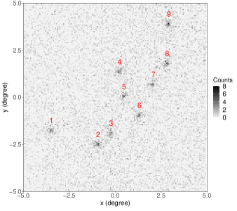
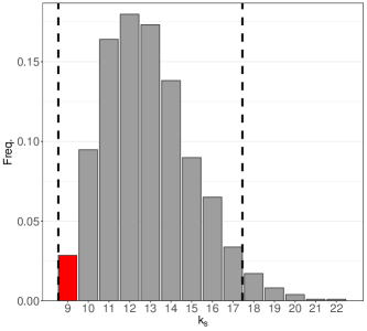


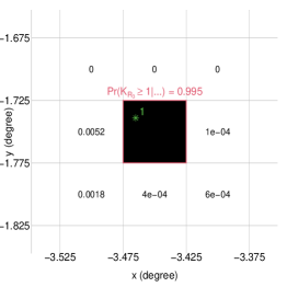


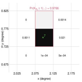
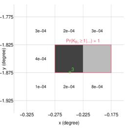
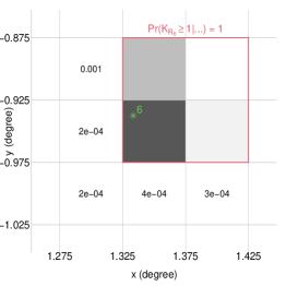

We run four separate Markov chains of length 10,000 in parallel using Algorithm 1, and discard the first three quarters of each as burn-in. The remaining draws are then combined to obtain a final posterior sample of the model parameters. The right panel of Figure 4 displays the posterior distribution of the number of sources, , and the 95% highest posterior density (HPD) interval (dashed vertical lines). The HPD interval indicates that there are between 9 and 17 sources, with a maximum a posteriori estimate of 12. Deploying Algorithm 3 using the same grid of pixels of size used to simulate the data, we examine the 12 distinct regions of the map, : Figure 5 shows these regions, delimited by red lines, together with their surrounding pixels. For every region, , that is, the probability that the region contains overlapping sources is negligible. Pixels within the regions are colour-coded according to the posterior distribution of , given for all . If follows that, if consists of a single pixel, the probability distribution of is concentrated within that pixel.
The first nine regions of Figure 5 contain the nine actual locations of the simulated sources (indicated by green stars); the probabilities under our model are , for . By contrast, the last three regions do not include any of the simulated point sources, and indeed the posterior probability that each contains a source is small, i.e., , for .
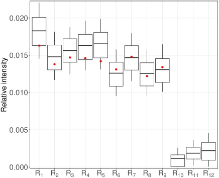
Figure 6 displays the posterior distribution of the relative intensities of the sources, which equal the product of and DP weights of , within the 12 regions. Red points denote the simulated proportion of photons generated by the 9 sources. Seven of the nine true proportions fall within the 68% HPD intervals, with the remaining two falling within the 95% HPD intervals. These results validate the capability of our method to identify sources in a relatively simple context.
4.3 More challenging simulations and model comparison
We carry out three additional simulation experiments to evaluate the ability of our method to identify sources in scenarios of growing complexity. In particular, we test whether including energy information substantially improves performance. We simulate 3 datasets (scenarios), each containing 15 point sources. The locations of the sources do not change across the datasets. Scenario 1 is simulated with and for ; this is thus identical to the illustrative example in Section 4.2 but with a larger number of sources. Scenario 2 is simulated with , for each , but different values of , sampled at random from the third Fermi LAT catalogue (3FGL) (Acero et al., 2015). This scenario provides a check of the importance of inference model misspecification in the spectral domain; recall that, unlike this simulation model, our inference model assumes that all point sources share the same spectral shape parameter. Scenario 3 is simulated with varying source brightnesses by setting to a sequence of 15 equispaced values between and , while , for each . Scenario 3 is useful to assess the performance of the Joint Spatial-Spectral Model relative to the simpler Spatial Model. Moderate contamination is simulated from the same background model used in Section 4.2 and added to the three datasets. Finally, the simulated photon counts are again thinned to 10,000 by random sampling in order to reduce the computational cost. The three maps and the background model used to generate the contamination appear in Appendix B, Figure 12.
We fit both the Spatial Model and the Joint Spatial-Spectral Model to all three simulation scenarios using the same hyperparameters and MCMC settings as in Section 4.2. For inference, we set the prior distribution of to , so that the a priori mode of is one and its shortest 95%-probability interval is (0, 3). This choice reflects the actual knowledge on sources with power-law spectra, which are known to have a shape parameter , that corresponds to in our Pareto model. We further set the prior of to , which has a priori approximately the same mode of , but twice the size of the 95% HPD interval. This choice reflects the lack of knowledge that we have on the spectral shape parameter of the background.
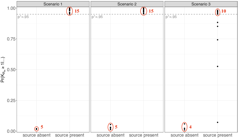
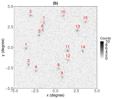
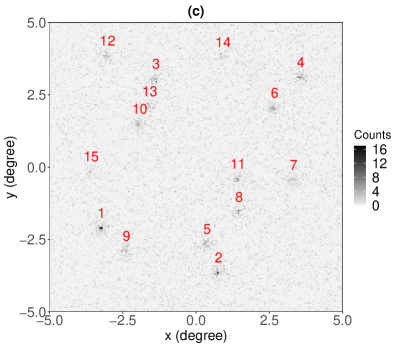
The results are shown in Figure 7. In Scenario 1, the 15 sources are identified with large probability (, as in Algorithm 3). Five 5 spurious regions also appear, but with very small probability of containing a source. Similar results are obtained for Scenario 2. For Scenario 3, 10 of the 15 sources are identified with probability above the threshold ; however, the remaining 5 sources are detected with probabilities less than , meaning that the model struggles to detect faint signals.
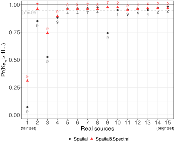
We do not display results from Scenario 1 and 2 from the Joint Spatial-Spectral Model as they are similar to those from Spatial Model; however, results for Scenario 3 differ substantially and worth exploring in detail. For Scenario 3, both models identify actual sources from the simulation along with spurious sources; Figure 8 displays only the actual sources. The x-axis sorts the regions in increasing order of source amplitude (so, corresponds to the source with the smallest amplitude, , and to the largest amplitude, ), and the y-axis gives , the probability of the region containing a source. Black circles are the probabilities under the Spatial Model, and red triangles under Joint Spatial-Spectral Model. Finally, the colored labels give the region sizes, expressed in number of pixels.
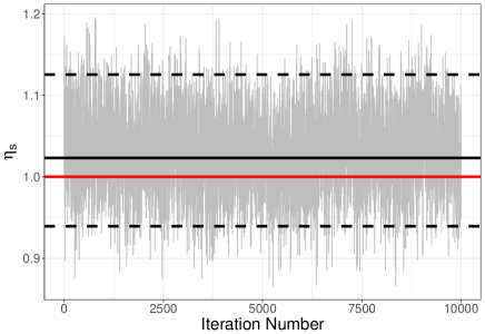
We notice that the Joint Spatial-Spectral Model performs considerably better than the Spatial Model in three different aspects. First, it recovers a higher proportion of the 15 sources and with high probability; 12 regions have probability , against the 10 regions from the Spatial Model with probability . Second, it returns smaller (that is, better localized) regions, allowing for a more precise evaluation of the source locations. Finally, it correctly extracts the true shape parameter of the sources , as demonstrated by the posterior traceplot of (see Figure 13 in Appendix B). This result is particularly notable, showing that the fitted source spectrum is consistent with the spectra used to generate the data even though both the image and spectral models of the background are misspecified. In addition to the actual simulation sources, the Joint Spatial-Spectral Model detects 4 spurious sources; however, their probability is low. (see left panel of Figure 13 in Appendix B).
To conclude, we confirm the ability of our inferential models to identify sources under scenarios of various complexity. Scenario 3 confirms that, like in Jones et al. (2015), the inclusion of energy brings noteworthy improvements in the accuracy of the source detection. These results encourage future extensions of the Joint Spatial-Spectral Model, which would, for example, account for sources with different shape parameters or extend the energy range by explicitly including the energy-dependent effective area.
5 Application to Fermi-LAT data
In this section, we apply our methods to -ray data collected over a 9.4 year period by the Fermi LAT from a region surrounding the newly discovered dwarf galaxy Antlia 2 (Torrealba et al.,, 2019), a potentially interesting target for dark matter-induced -ray emission. This region is relatively close to the Galactic plane, and therefore subject to significant diffuse background processes that have strong gradients across the field of view. A first background model developed by the Fermi Collaboration (Acero et al., 2016) is made up of an isotropic component plus a diffuse component representing diffuse galactic emission. The physical processes that give rise to the diffuse emission are difficult to model and we do not expect the Fermi background model to capture all the detailed morphological and spectral characteristics of the true background. Therefore, a method independent from the Fermi background model would be more suitable for estimating the noise component of the data.
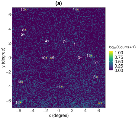
The original Fermi dataset contains the photons from a region of spatial pixels of size , across 30 energy pixels in the range . To reduce computational cost, we restricted our attention to an area at the centre of the image of size pixels, and we removed photons with energies less than . The resultant dataset consists of 23,897 photons and is illustrated in Figure 9(a). Strong emission from the Galactic plane is visible at the bottom of the map; this background emission progressively diminishes toward northern latitudes (top of the figure), away from the Galactic plane. The latest Fermi LAT source catalogue (4FGL) (Abdollahi et al.,, 2020) reports 16 sources in this area, denoted by red circles and labelled in ascending order according to their expected photon count in the energy range . Thus, we expect the smallest photon count from Source 1, and the largest from Source 16.
We fit both the Spatial Model and the Joint Spatial-Spectral Model with the same prior set-up described in Section 4.3. For both models, we run four separate Markov chains, each of length 10,000, and discard the first three quarters of each chain as burn-in. The remainder are combined to form a posterior sample of size 10,000. The simulations were implemented in the R language and environment for statistical computing (R Core Team,, 2020). The four chains were run in parallel on the departmental computer cluster and took approximately one day to produce the results.

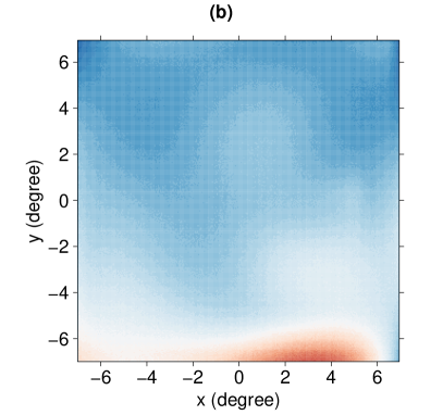
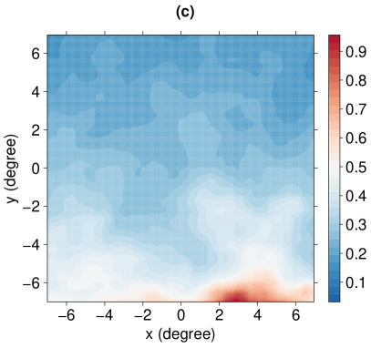
Figure 9(b) shows the posterior expected counts per pixel from background under our B-spline DP mixture. We generate this map by simulating, for every iteration of the posterior sample, photon counts from (4) with parameters evaluated at iteration , and then binning them into the grid of pixels. Averaging across the 10,000 iterations of the posterior sample gives a Monte Carlo estimate of the posterior expected pixel counts. In contrast, Figure 9(c) shows the expected photon counts under the Fermi collaboration model, which is a single “best-fit” model to the entire -ray sky. The two panels broadly agree in identifying (i) a prominent contamination from the nearby Galactic plane at southern latitudes (bottom of the images), (ii) some moderate and more uniform background areas in the middle of the maps, and (iii) a considerably reduced background contribution moving to northern latitudes (top of the images). Nevertheless, our method gives substantially lower expected counts in the bottom-right corner of the map than does the Fermi model. This discrepancy occurs because our model fit indicates two potential sources in this region, whereas the Fermi background model subsumes these potential sources. We return to this point below. Our expected background, shown in Figure 9(b), also appears smoother than the Fermi background of Figure 9(c). This is because our model adapts to the varying background morphology, unlike the fixed Fermi model, which pixel-wise estimates the background without uncertainty. Under our mixture model we have access not just to the marginal expected pixel counts but to the joint distribution of counts in all pixels, allowing us, for example, to explore spatial correlations in the background structure. Additionally, the detailed, small-scale features in the Fermi background map (Figure 9(c)) are not detected in the -ray data. Rather, they correspond to patterns of gas clumps present in templates (see Section 1.1). By contrast, our B-spline background model only includes “features” that can be inferred from the -ray data.
Both the Spatial Model and the Joint Spatial-Spectral Model detect nine of the 16 sources listed by the Fermi catalogue (IDs 8-16), see Figure 10. The Joint Spatial-Spectral Model performs considerably better than the Spatial Model, providing higher posterior probabilities and smaller regions for eight sources. (The only exception is Source 12.) This result is encouraging, especially considering that, according to Abdollahi et al., (2020), the sources in questions have substantially different spectral shapes, which is something that our Joint Spatial-Spectral Model does not account for.


Although we do not detect Sources 1-7, Abdollahi et al., (2020) reports that these sources are of low brightness ( for the brightest of them), and their spectra have a steep power-law (). Thus, we expect a small number of photons from each, and mostly at low energies. We may detect these sources if we include photons with energies less than 1 GeV as done in Abdollahi et al., (2020).
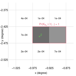
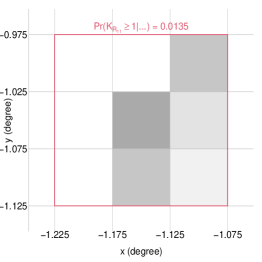
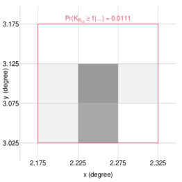
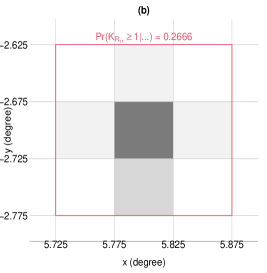
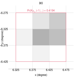
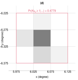
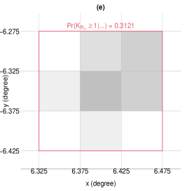
Our analysis identified four additional point sources not recorded in the Fermi catalogue; details are given in Figure 11. In particular, both the Spatial Model and the Joint Spatial-Spectral Model indicate the presence of points sources in the same regions in the bottom-right corner of the map. The first appears in Figure 11(a) and Figure 11(d), with probabilities of 0.43 and 0.48 respectively. The second appears in Figure 11(c) and Figure 11(e) with probabilities of 0.42 and 0.31. The third region discovered by the Spatial Model (Figure 11(b)) has presumably recovered a faint signal from Source 6, as it is away from its catalogue location (see Figure 9(a)). However, we conclude there is no source in this region as its probability is only 0.26. Lastly, there is a third region in the bottom-right corner of the map indicated by the Joint Spatial-Spectral Model (Figure 11(f)): since its probability of including a source is 0.13, we consider it spurious.
6 Discussion
We present an innovative approach to extract point sources in highly contaminated high-energy (-ray and X-ray) photon-count maps using both spatial and spectral information. The methods exploit advanced Bayesian nonparametric techniques in a way that simultaneously identifies point sources and fits the background contamination. A physics-based constraint on the background parameter space is imposed to reduce the possibility that the signal of some sources is attributed to the background. Our mixture of DP mixture models is fitted to the data via Markov chain Monte Carlo simulation. In addition, we developed a post-processing algorithm that conducts inference on component-specific parameters, even when some posterior distributions are multimodal, and handles the well-known label switching problem in mixture models. We further illustrated its working with examples drawn from real astrophysical applications.
We proposed two models: the first exploits only the spatial information of the photons, the second extends it in a simple manner by including the energy, as well, under the simplifying assumptions that all sources share the same power-law spectrum. The two models exhibited good detection performance on several simulation experiments of growing complexity, and revealed only few spurious clusters which could be easily recognised using the posterior probability of corresponding to real sources computed with the proposed algorithm for posterior analysis. Simulation experiments have also shown that the extended model is better suited to extracting point sources when they all share a similar spectral shape parameter.
Finally, we carried out the analysis of a real-case dataset, a map of photons collected by the Fermi LAT space observatory around the newly discovered galaxy Antlia-2. As revealed by the comparison with the Fermi collaboration background model (Acero et al., 2016), our B-spline DP mixture is able to reconstruct the background morphology, thus demonstrating its ability to detect and separate point sources from background emission in highly contaminated maps. We successfully extracted the signal of 9 sources, whose presence was already known from the last Fermi catalogue, and we identified additional regions where point sources may be present, and which do not coincide with any known source. The Joint Spatial-Spectral Model model performed considerably better than the Spatial Model even if the discovered sources are known to have different spectral parameters. Our results from both simulated experiments and real-case data definitely encourage future extensions of the Joint Spatial-Spectral Model model in two different directions: first, allowing the source DP mixture to model the spectrum of multiple sources with different spectral parameters, and second, providing ad adequate model for the background energy.
With respect to the finite mixture approach of Jones et al. (2015), DP mixtures have both conceptual and computational advantages. Considering that the number of components in Bayesian nonparametric mixtures is potentially infinite, a larger number of records usually implies a larger size of the mixture. Thus, a DP-based model looks more appropriate than a finite mixture as, with sky surveys, new data become available and may guide to the identification of new sources that could not be recognized before. Moreover, the available algorithms for nonparametric Bayes models look more efficient for posterior inference and scale the mixture size faster than the reversible jump algorithm.
Appendix A Gibbs sampler for B-spline knots
Let , with , be the coordinates of the longitude for photons which are bounded into the interval . Let us assume they distribute according to the density , with a five-dimensional vector of longitude knots. At the -th iteration of the MCMC algorithm, the full-conditional density of is
where if , if and if . Furthermore, is the vector without its -th element. Recall the base measure given in Section 2.3. Then, for :
-
1.
let be the lower and the upper bounds of given by Table 1, and
-
2.
draw and . If
and satisfies the constraint on the B-spline variance (8), then . Otherwise, reject and repeat Step 2.
The same sampling scheme can be adopted to draw also from the posterior distribution of the latitude knots b by replacing with .
| Knot | Left bound | Right bound |
Appendix B Additional results from Section 4.2

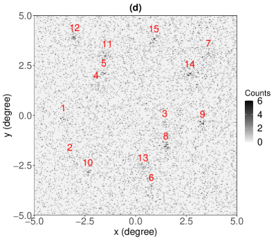
This section contains some additional graphs related to the simulation experiments conducted in Section 4.3. Figure 12(a) shows the expected photon counts of the background model by Acero et al. (2016) which we used to simulate the background data for the experiments of Sections 4.2 and 4.3. Panels (b-d) show the three simulated datasets of Section 4.3. The sources in the three scenario are labelled with different criteria. In Scenario 1, they are labelled from 1 to 15 according to increasing longitude. In Scenario 2, they are labelled according to the spectral shape parameter : Source 1 has the shallowest spectrum () and Source 15 has the steepest spectrum (). Last, in Scenario 3, Source 1 is the faintest source () and Source 15 the brightest () one.
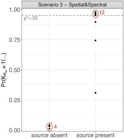
The left panel of Figure 13 displays the regions discovered under the Joint Spatial-Spectral Model for Scenario 3, differentiated according to whether they do (“source present”) or do not (“source absent”) include a real source. The right panel displays the traceplot of obtained from a MCMC run of length 10,000. The red line is the spectral shape parameter of the 15 simulated sources, rescaled by 1 to match the parametrization of the Pareto density function (in fact, ). The posterior mode and the 95% HPD interval are also displayed using solid and dashed black lines, respectively.
Acknowledgements
The authors thank Antonio Canale and Michele Guindani for their many useful discussions and constructive comments. This project was supported by SID grant “Advanced statistical modelling for indexing celestial objects” (BIRD185983) awarded by the Department of Statistical Sciences of the University of Padova. This work was conducted in collaboration with the CHASC International Astrostatistics Center. CHASC is supported by NSF DMS-18-11308, DMS-18-11083, and DMS-18-11661. We thank CHASC members for many helpful discussions. DvD’s and RT’s work was supported in part by a Marie-Skodowska-Curie RISE (H2020-MSCA-RISE-2015-691164, H2020-MSCA-RISE-2019-873089) Grants provided by the European Commission. RT’s work was partially supported by STFC under grant number ST/T000791/1.
References
- Abazajian et al., (2020) Abazajian, K. N., Horiuchi, S., Kaplinghat, M., Keeley, R. E., and Macias, O. (2020). Strong constraints on thermal relic dark matter from Fermi-LAT observations of the Galactic Center. Physical Review D, 102(4):043012.
- Abdollahi et al., (2020) Abdollahi, S., Acero, F., Ackermann, M., Ajello, M., Atwood, W., Axelsson, M., Baldini, L., Ballet, J., Barbiellini, G., Bastieri, D., et al. (2020). Fermi large area telescope fourth source catalog. The Astrophysical Journal Supplement Series, 247(1):33.
- Acero et al. (2015) Acero, F., Ackermann, M., Ajello, M., Albert, A., Atwood, W., Axelsson, M., Baldini, L., Ballet, J., Barbiellini, G., Bastieri, D. et al. (2015) Fermi large area telescope third source catalog. The Astrophysical Journal Supplement Series 218(2), 23–63.
- Acero et al. (2016) Acero, F., Ackermann, M., Ajello, M., Albert, A., Baldini, L., Ballet, J., Barbiellini, G., Bastieri, D., Bellazzini, R., Bissaldi, E. et al. (2016) Development of the model of galactic interstellar emission for standard point-source analysis of Fermi large area telescope data. The Astrophysical Journal Supplement Series 223(2), 26–48.
- Ackermann et al. (2012) Ackermann, M., Ajello, M., Albert, A., Allafort, A., Atwood, W., Axelsson, M., Baldini, L., Ballet, J., Barbiellini, G., Bastieri, D. et al. (2012) The Fermi large area telescope on orbit: event classification, instrument response functions, and calibration. The Astrophysical Journal Supplement Series 203(1), 4–73.
- Biller (2000) Biller, C. (2000) Adaptive Bayesian regression splines in semiparametric generalized linear models. Journal of Computational and Graphical Statistics 9(1), 122–140.
- Blackwell (1973) Blackwell, D. (1973) Discreteness of Ferguson selections. Annals of Statistics 1, 356–358.
- Bush and MacEachern, (1996) Bush, C. A. and MacEachern, S. N. (1996). A semiparametric Bayesian model for randomised block designs. Biometrika, 83(2), 275–285.
- Carlson (1991) Carlson, B. C. (1991) -splines, hypergeometric functions, and Dirichlet averages. Journal of Approximation Theory 67(3), 311–325.
- Costantin et al., (2020) Costantin, D., Sottosanti, A., Brazzale, A. R., Bastieri, D., and Fan, J. (2020). Bayesian mixture modelling of the high-energy photon counts collected by the Fermi Large Area Telescope. Statistical Modelling, 0(0):1471082X20947222.
- Daylan et al., (2017) Daylan, T., Portillo, S. K., and Finkbeiner, D. P. (2017). Inference of unresolved point sources at high galactic latitudes using probabilistic catalogs. The Astrophysical Journal, 839(1):4.
- de Boor (2001) de Boor, C. (2001) A practical guide to splines. Revised edition, volume 27 of Applied Mathematical Sciences. Springer-Verlag, New York.
- Denison et al. (1998) Denison, D. G. T., Mallick, B. K. and Smith, A. F. M. (1998) Automatic Bayesian curve fitting. Journal of the Royal Statistical Society Series B 60(2), 333–350.
- DiMatteo et al. (2001) DiMatteo, I., Genovese, C. R. and Kass, R. E. (2001) Bayesian curve-fitting with free-knot splines. Biometrika 88(4), 1055–1071.
- Do et al., (2005) Do, K.-A., Müller, P., and Tang, F. (2005). A Bayesian mixture model for differential gene expression. Journal of the Royal Statistical Society Series C, 54(3), 627–644.
- Escobar (1994) Escobar, M. D. (1994) Estimating normal means with a Dirichlet process prior. Journal of the American Statistical Association 89(425), 268–277.
- Escobar and West (1995) Escobar, M. D. and West, M. (1995) Bayesian density estimation and inference using mixtures. Journal of American Statistical Association 90(430), 577–588.
- Ferguson (1973) Ferguson, T. S. (1973) A Bayesian analysis of some nonparametric problems. Annals of Statistics 1, 209–230.
- Feroz and Hobson, (2008) Feroz, F. and Hobson, M. P. (2008). Multimodal nested sampling: an efficient and robust alternative to Markov Chain Monte Carlo methods for astronomical data analyses. Monthly Notices of the Royal Astronomical Society, 384(2), 449–463.
- Frühwirth-Schnatter, (2011) Frühwirth-Schnatter, S. (2011). Dealing with label switching under model uncertainty. In Mixtures: estimation and applications, Wiley Ser. Probab. Stat., pages 213–239. Wiley, Chichester.
- Guglielmetti et al. (2009) Guglielmetti, F., Fischer, R. and Dose, V. (2009) Background–source separation in astronomical images with Bayesian probability theory – I. The method. Monthly Notices of the Royal Astronomical Society 396(1), 165–190.
- Hobson et al. (2010) Hobson, M. P., Jaffe, A. H., Liddle, A. R., Mukherjee, P. and Parkinson, D. (eds) (2010) Bayesian methods in cosmology. Cambridge University Press, Cambridge.
- Jones et al. (2015) Jones, D. E., Kashyap, V. L. and van Dyk, D. A. (2015) Disentangling overlapping astronomical sources using spatial and spectral information. The Astrophysical Journal 808(2), 137–160.
- Knoetig (2014) Knoetig, M. L. (2014) Signal discovery, limits, and uncertainties with sparse on/off measurements: An objective Bayesian analysis. The Astrophysical Journal 790(2), 106–113.
- Koposov et al., (2018) Koposov, S. E., Walker, M. G., Belokurov, V., Casey, A. R., Geringer-Sameth, A., Mackey, D., Da Costa, G., Erkal, D., Jethwa, P., Mateo, M., Olszewski, E. W., and Bailey, J. I. (2018). Snake in the Clouds: a new nearby dwarf galaxy in the Magellanic bridge. Monthly Notices of the Royal Astronomical Society, 479(4), 5343–5361.
- Kraft et al. (1991) Kraft, R. P., Burrows, D. N. and Nousek, J. A. (1991) Determination of confidence limits for experiments with low numbers of counts. The Astrophysical Journal 374(1), 344–355.
- Lauritzen and Spiegelhalter, (1988) Lauritzen, S. L. and Spiegelhalter, D. J. (1988). Local computations with probabilities on graphical structures and their application to expert systems. Journal of the Royal Statistical Society Series B, 50(2), 157–224. With discussion.
- Liu, (1994) Liu, J. S. (1994). The collapsed Gibbs sampler in Bayesian computations with applications to a gene regulation problem. Journal of the American Statistical Association, 89(427), 958–966.
- MacEachern and Müller, (1998) MacEachern, S. N. and Müller, P. (1998). Estimating Mixture of Dirichlet Process Models. Journal of Computational and Graphical Statistics, 7(2), 223–238.
- Mattox et al. (1996) Mattox, J. R., Bertsch, D., Chiang, J., Dingus, B., Digel, S., Esposito, J., Fierro, J., Hartman, R., Hunter, S., Kanbach, G. et al. (1996) The likelihood analysis of EGRET data. The Astrophysical Journal 461, 396–407.
- Meyer et al. (2021) Meyer, A. D., van Dyk, D. A., Kashyap, V. L., Campos, L. F., Jones, D. E., Siemiginowska, A., Meng, X.-L., and Zezas, A. (2021) Probabilistic disentanglement of overlapping x-ray sources by space, time, and energy. Preprint
- Müller et al. (2015) Müller, P., Quintana, F. A., Jara, A. and Hanson, T. (2015) Bayesian nonparametric data analysis. Springer Series in Statistics. Springer, Cham.
- Müller and Rodriguez (2013) Müller, P. and Rodriguez, A. (2013) Nonparametric Bayesian inference. Volume 9 of NSF-CBMS Regional Conference Series in Probability and Statistics. Institute of Mathematical Statistics, Beachwood, OH; American Statistical Association, Alexandria, VA.
- Neal (2000) Neal, R. M. (2000) Markov chain sampling methods for Dirichlet process mixture models. Journal of Computational and Graphical Statistics 9(2), 249–265.
- Park et al. (2006) Park, T., Kashyap, V. L., Siemiginowska, A., van Dyk, D. A., Zezas, A., Heinke, C. and Wargelin, B. J. (2006) Bayesian estimation of hardness ratios: Modeling and computations. The Astrophysical Journal 652(1), 610–628.
- Primini and Kashyap (2014) Primini, F. A. and Kashyap, V. L. (2014) Determining x-ray source intensity and confidence bounds in crowded fields. The Astrophysical Journal 796(1), 24–37.
- Protassov et al. (2002) Protassov, R., van Dyk, D. A., Connors, A., Kashyap, V. L. and Siemiginowska, A. (2002) Statistics, handle with care: detecting multiple model components with the likelihood ratio test. The Astrophysical Journal 571(1), 545–559.
- Ray et al. (2011) Ray, P. S., Kerr, M., Parent, D., Abdo, A., Guillemot, L., Ransom, S., Rea, N., Wolff, M., Makeev, A., Roberts, M. et al. (2011) Precise -ray timing and radio observations of 17 Fermi -ray pulsars. The Astrophysical Journal Supplement Series 194(2), 17–44.
-
R Core Team, (2020)
R Core Team (2020). R: A Language and Environment for Statistical Computing. R Foundation for Statistical Computing, Vienna, Austria.
https://www.R-project.org/ - Richardson and Green, (1997) Richardson, S. and Green, P. J. (1997). On Bayesian analysis of mixtures with an unknown number of components. Journal of the Royal Statistical Society Series B, 59(4), 731–792.
- Savage and Oliver, (2007) Savage, R. S. and Oliver, S. (2007). Bayesian Methods of Astronomical Source Extraction. The Astrophysical Journal, 661(2), 1339–1346.
- Schellhase and Kauermann (2012) Schellhase, C. and Kauermann, G. (2012) Density estimation and comparison with a penalized mixture approach. Computational Statistics 27(4), 757–777.
- Selig and Enßlin (2015) Selig, M. and Enßlin, T. A. (2015) Denoising, deconvolving, and decomposing photon observations. Derivation of the D3PO algorithm. Astronomy & Astrophysics 574, A74.
- Selig et al. (2015) Selig, M., Vacca, V., Oppermann, N. and Enßlin, T. A. (2015) The denoised, deconvolved, and decomposed Fermi -ray sky-An application of the D3PO algorithm. Astronomy & Astrophysics 581, A126.
- Sharef et al. (2010) Sharef, E., Strawderman, R. L., Ruppert, D., Cowen, M. and Halasyamani, L. (2010) Bayesian adaptive B-spline estimation in proportional hazards frailty models. Electronic Journal of Statitics 4, 606–642.
- Stein et al. (2015) Stein, N. M., van Dyk, D. A., Kashyap, V. L. and Siemiginowska, A. (2015) Detecting unspecified structure in low-count images. The Astrophysical Journal 813(1), 66–80.
- Torrealba et al., (2019) Torrealba, G., Belokurov, V., Koposov, S. E., Li, T. S., Walker, M. G., Sanders, J. L., Geringer-Sameth, A., Zucker, D. B., Kuehn, K., Evans, N. W., and Dehnen, W. (2019). The hidden giant: discovery of an enormous Galactic dwarf satellite in Gaia DR2. Monthly Notices of the Royal Astronomical Society, 488(2).
- van Dyk et al. (2001) van Dyk, D. A., Connors, A., Kashyap, V. L. and Siemiginowska, A. (2001) Analysis of energy spectra with low photon counts via Bayesian posterior simulation. The Astrophysical Journal 548(1), 224–243.
- Weisskopf et al. (2007) Weisskopf, M. C., Wu, K., Trimble, V., O’Dell, S. L., Elsner, R. F., Zavlin, V. E. and Kouveliotou, C. (2007) A Chandra search for coronal x-rays from the cool white dwarf gd 356. The Astrophysical Journal 657(2), 1026–1036.