Development of Advanced Linearized Gyrokinetic Collision Operators Using a Moment Approach

Abstract

The derivation and numerical implementation of a linearized version of the gyrokinetic (GK) Coulomb collision operator (Jorge R. et al., J. Plasma Phys. 85, 905850604 (2019)) and of the widely-used linearized GK Sugama collision operator (Sugama H. et al., Phys. Plasmas 16, 112503 (2009)) is reported. An approach based on a Hermite-Laguerre moment expansion of the perturbed gyrocenter distribution function is used, referred to as gyro-moment expansion. This approach allows considering arbitrary perpendicular wavenumber and expressing the two linearized GK operators as a linear combination of gyro-moments where the expansion coefficients are given by closed analytical expressions that depend on the perpendicular wavenumber and on the temperature and mass ratios of the colliding species. The drift-kinetic (DK) limits of the GK linearized Coulomb and Sugama operators are also obtained. Comparisons between the gyro-moment approach and the DK Coulomb and GK Sugama operators in the continuum GK code GENE are reported, focusing on the ion-temperature-gradient instability and zonal flow damping, finding an excellent agreement. It is confirmed that stronger collisional damping of the zonal flow residual by the Sugama GK model compared to the GK linearized Coulomb (Pan Q. et al., Phys. Plasmas 27, 042307 (2020)) persists at higher collisionality. Finally, we show that the numerical efficiency of the gyro-moment approach increases with collisionality, a desired property for boundary plasma applications.

1 Introduction

Understanding the plasma dynamics of the tokamak boundary is necessary to address some of the most crucial problems fusion is facing today and, for instance, to ensure the success of future devices, such as ITER (Shimada et al., 2007; Holtkamp, 2009). In fact, the boundary region, which extends from the external part of the closed flux surface region (typically referred to as the edge) to the scrape-off layer (SOL) where the magnetic field lines intercept the machine vessel walls, sets the particle and heat exhaust, helium ash removal and the overall confinement of the device. Most often, drift-reduced fluid models (see, e.g., (Zeiler et al., 1997)) implemented in a number of simulation codes (Dudson et al., 2009; Tamain et al., 2016; Halpern et al., 2016; Paruta et al., 2018; Zhu et al., 2018; Stegmeir et al., 2019; Giacomin et al., 2020) are used to simulate SOL turbulence. However, the applicability of Braginskii-like fluid models is questionable to describe the whole boundary region, since they assume $k_{\parallel}\lambda_{mpf}\ll 1$ and $k_{\perp}\rho_{i}\ll 1$, where $k_{\parallel}$ and $k_{\perp}$ are the parallel and perpendicular components of the wavevector $\bm{k}$ to the equilibrium magnetic field lines, $\lambda_{mfp}$ is the electron mean free path, and $\rho_{i}$ is the ion Larmor radius. In particular, the $k_{\parallel}\lambda_{mpf}\ll 1$ assumption is expected to no longer be satisfied in larger and hotter machines near and inside of the edge, like ITER (Holtkamp, 2009). For this reason, an enormous effort is being carried out by the fusion community to extend core gyrokinetic (GK) codes, which are based on PIC or grid-based methods (Dimits et al., 1996; Idomura et al., 2003; Görler et al., 2011; Villard et al., 2013; Chang et al., 2017), to simulate the boundary region. However, despite large recent progress, the application of core GK models and codes in the boundary region is challenged, for instance, by the nature of collisions. Collisions are expected to play an important role in the boundary region as they can substantially affect the properties of trapped electron (TEM) and ion temperature gradient (ITG) modes (Belli & Candy, 2017), the suppression of short wavelength structure (Barnes et al., 2009), TEM turbulent fluxes, the damping of zonal flows (Pan et al., 2020, 2021), and the growth rate of pedestal microtearing modes (Pan et al., 2021).

An accurate description of binary Coulomb collisions dominated by small angle deflection is provided by the nonlinear Fokker-Planck operator, that we refer to as the Coulomb collision operator (Rosenbluth et al., 1957). The nonlinear Coulomb collision operator is an integro-differential operator that acts on the full particle distribution function. Because of the complexity of the nonlinear Coulomb collision operator, its version linearized around a Maxwellian distribution function is usually considered (Rosenbluth et al., 1957; Helander & Sigmar, 2002; Hazeltine & Meiss, 2003). However, despite being simpler than the nonlinear collision operator, the numerical implementation of the linearized Coulomb collision operator is still challenging. This inherent difficulty primarily stems in the evaluation of the component of the linearized collision operator that contains velocity space integrals of the perturbed distribution function. As a matter of fact, it is only recently that the implementation of a linearized GK Coulomb collision operator has been reported in the GK GENE code (Pan et al., 2020, 2021).

Because of the complexity associated with dealing with the Coulomb collision operator, simplified model collision operators have been developed (Dougherty, 1964; Hirshman & Sigmar, 1976; Abel et al., 2008; Sugama et al., 2009, 2019). In particular, Sugama et al. (2009) derived an approximated linearized collision operator, that we refer to as the Sugama operator, extending the work of Abel et al. (2008) to multiple ion species plasmas. This operator is designed such that it conserves particle, momentum and energy and, in addition, it fulfils the self-adjoint relations for unlike-species, a useful property when solving collisional transport problems based on the drift-kinetic equation (Rosenbluth et al., 1972). While the Sugama operator have been tested in neoclassical and turbulent studies at low collisionalities (Nakata et al., 2015; Nunami et al., 2015), its deviation with respect to the Coulomb operator (Crandall et al., 2020; Pan et al., 2020, 2021) is expected to increase when applied at higher collisionalities, such as the ones in the plasma boundary. We remark that the first GK Coulomb operators with exact field terms rather than simplified models, including finite Larmor radius effects, were formulated in Li & Ernst (2011); Madsen (2013); Pan & Ernst (2019); Jorge et al. (2019).

Advanced numerical algorithms have been developed for the implementation of these collision operators (Xu & Rosenbluth, 1991; Dimits & Cohen, 1994; Barnes et al., 2009; Landreman & Ernst, 2012, 2013; Nakata et al., 2015; Hager et al., 2016; Belli & Candy, 2017; Crandall et al., 2020; Pan et al., 2020), since numerical errors can potentially yield spurious noise and break the conservation laws producing artificial instabilities. Among the different numerical schemes, Monte-Carlo techniques are used in some PIC codes (Xu & Rosenbluth, 1991; Dimits & Cohen, 1994; Kolesnikov et al., 2010), while GK continuum codes and some PIC codes adopt velocity-space grid-based discretization method (Dorf et al., 2014; Hager et al., 2016; Pan et al., 2020; Crandall et al., 2020). We remark that, recently, a novel conservative discontinuous Galerkin method has been developed and applied to a nonlinear Dougherty collision operator in Francisquez et al. (2020), and present the potential of being generalized to more advanced collision operators. Novel spectral methods have yielded significant improvements in accuracy and speed in neoclassical and gyrokinetic codes (Landreman & Ernst, 2012, 2013; Held et al., 2015; Belli & Candy, 2017). Also, orthogonal polynomials expansion techniques have been used in the numerical treatment of velocity-space derivatives (Donnel et al., 2019).

Recently, to provide a theoretical and numerical framework able to predict and study efficiently the dynamics of the boundary region, a GK model valid at an arbitrary level of collisionality has been developed by Frei et al. (2020). This model is based on expanding the full distribution function on a Hermite-Laguerre polynomial basis. By projecting the GK equation onto the same basis, the evolution of the distribution function is reduced to the one of the coefficients of its expansion, referred to as gyro-moments. To describe collisional effects, while Frei et al. (2020) presents a nonlinear full-F GK Dougherty collision operator for like-species, a nonlinear full-F Coulomb collision operator has been derived in Jorge et al. (2019) using the same Hermite-Laguerre gyro-moment approach. This operator is valid at arbitrary wavelengths perpendicular to the magnetic field, and arbitrary mass and temperature ratios. Coupled with the full-F nonlinear GK operator in Jorge et al. (2019), the gyro-moment hierarchy in Frei et al. (2020) reduces, in the DK limit, to an improved set of Braginskii-like fluid equations where only the lowest order gyro-moments are considered (Jorge et al., 2017), while a progressively more detailed kinetic representation is obtained by increasing the number of gyro-moments.

The goal of the present paper is twofold. First, we derive the linearized GK Coulomb collision and the GK Sugama operators within the Hermite-Laguerre gyro-moment expansion. For treating the case of the GK Coulomb collision operator, we leverage the techniques introduced by Jorge et al. (2019). Using a spherical harmonic moment expansion technique of the particle distribution function, we perform the gyro-average of the linearized Coulomb operator analytically, removing the fast particle gyro-motion, and project the result onto the Hermite-Laguerre basis. One of the advantages of the Hermite-Laguerre decomposition is that it allows one to reduce velocity integrals in the linearized collision operators, which are treated numerically in, e.g., (Pan et al., 2020; Crandall et al., 2020), to closed algebraic expressions that depend only on the perpendicular wavenumber, on the temperature and mass ratios of the colliding species and on the gyro-moments. The DK limits of the GK Coulomb and Sugama operators are also derived. Second, expressed in a form suitable for a numerical treatment, we implement these operators in a numerical simulation code. We test and compare the GK Sugama and DK Coulomb collision operators against the widely-used gyrokinetic continuum code GENE (Jenko et al., 2000), focusing on the ITG linear growth rate and collisional zonal flow damping. We report a good agreement with GENE, and show, in particular, that the new linearized GK Sugama produces a larger collisional damping of the ZF residual compared to the GK Coulomb. Finally, we illustrate the numerical efficiency of the gyro-moment approach against GENE as the collisionality increases, a desired property for boundary plasma applications. We remark that, while only valid for small deviations from equilibrium, the linearized GK operator presented in this work opens the way to a future numerical implementation of the full-F nonlinear GK Coulomb operator (Jorge et al., 2019).

The structure of the paper is the following. We first introduce the gyro-moment approach to the linearized gyrokinetic model in Section 2. In Section 3, we derive the Hermite-Laguerre expansion the linearized GK Coulomb and GK Sugama operators that we express in terms of gyro-moments. We describe the numerical implementations of the collision operators in Fig. 3. Then, we test the linearized GK collision operators considering the ion-temperature-gradient (ITG) instability and collisional damping of the zonal flow (ZF) residual in Section 5. By performing direct results comparisons with GENE, Section 6 illustrates the numerical efficiency of the gyro-moment approach as the collisionality increases. We conclude in Section 7.

2 Gyrokinetic Model Equation

We consider the electrostatic gyrokinetic Boltzmann equation in the presence of magnetic field, density and temperature gradients. We use the gyrocenter phase-space coordinates $\bm{Z}=(\bm{R},\mu,v_{\parallel},\theta)$, where $\bm{R}=\bm{r}-\bm{\rho}_{a}$ is the gyrocenter position (with $a$ the species index), with $\bm{r}$ the particle position and $\bm{\rho}_{a}(\bm{R},\mu,\theta)=\bm{b}\times\bm{v}/\Omega_{a}$ the gyroradius of species $a$ ($\bm{b}=\bm{B}/B$ and $\Omega_{a}=q_{a}B/m_{a}$), $\mu=m_{a}v_{\perp}^{2}/[2B(\bm{R})]$ is the magnetic moment, $v_{\parallel}=\bm{b}\cdot\bm{v}$ is the component of the velocity parallel to the magnetic field, and $\theta$ is the gyroangle. We linearize the GK Boltzmann equation by assuming that the gyrocenter distribution function of species $a$, $F_{a}=F_{a}(\bm{R},\mu,v_{\parallel})$, is a perturbed Maxwellian, that is $F_{a}=F_{Ma}+\textsl{g}_{a}$, with $\textsl{g}_{a}=\textsl{g}_{a}(\bm{R},\mu,v_{\parallel},t)$, the perturbation with respect to the local Maxwellian distribution function $F_{Ma}=Ne^{-s_{\parallel a}^{2}-x_{a}}/(\pi^{3/2}v_{Ta}^{3})$ such that $\textsl{g}_{a}/F_{Ma}\ll 1$,, with $N=N_{i}(\bm{R})=N_{e}(\bm{R})$ the background gyrocenter density, $s_{\parallel a}=v_{\parallel}/v_{Ta}(\bm{R})$, $x_{a}=\mu B(\bm{R})/T_{a}(\bm{R})$, and $v_{T_{a}}^{2}(\bm{R})=2T_{a}(\bm{R})/m_{a}$ the thermal velocity based on the equilibrium temperature $T_{a}(\bm{R})$. The linearized electrostatic GK Boltzmann equation that describes the time evolution of $\textsl{g}_{a}(\bm{k},t)=\int d\bm{R}\textsl{g}_{a}(\bm{R},t)e^{-i\bm{R}\cdot\bm{k}}$ can be written as (Hazeltine & Meiss, 2003)

$$\frac{\partial}{\partial t}\textsl{g}_{a} +i\omega_{Ba}h_{a}+v_{\parallel}\gradient_{\parallel}h_{a}-\frac{\mu}{m_{s}}(\bm{b}\cdot\gradient B)\frac{\partial}{\partial v_{\parallel}}h_{a}-i\omega_{Ta}^{*}J_{0}(b_{a}\sqrt{x_{a}})\phi F_{Ma}=\sum_{b}\mathcal{C}_{ab},$$ (1)

where $\phi=\phi(\bm{k},t)$ is the Fourier component of the electrostatic potential and we introduce the nonadiabatic part, $h_{a}=h_{a}(\bm{k},\mu,v_{\parallel},t)$, of the perturbed gyrocenter distribution function $\textsl{g}_{a}$, that is

$$h_{a}=\textsl{g}_{a}+\frac{q_{a}}{T_{a}}F_{Ma}J_{0}(b_{a}\sqrt{x_{a}})\phi.$$ (2)

In Eq. 1, we define $\gradient_{\parallel}=\bm{b}\cdot\gradient$, $\omega_{Ba}=v_{Ta}^{2}(x_{a}+2s_{\parallel a}^{2})\omega_{B}/(2\Omega_{a})$, with $\omega_{B}=\left(\bm{b}\times\gradient\ln B\right)\cdot\bm{k}$, and $\omega_{Ta}^{*}=\left[\omega_{N}+\omega_{T_{a}}\left(x_{a}+s_{\parallel a}^{2}-3/2\right)\right]$, with $\omega_{N}=\bm{b}\times\gradient\ln N\cdot\bm{k}/B$ and $\omega_{T_{a}}=\bm{b}\times\gradient\ln T_{a}\cdot\bm{k}/B$ . Finite Larmor radius (FLR) effects are taken into account through the zeroth order Bessel function, $J_{0}(b_{a}\sqrt{x_{a}})$, where $b_{a}=k_{\perp}v_{T_{a}}/\Omega_{a}$ is the normalized perpendicular wavevector, with $k_{\perp}=|\bm{k}-(\bm{b}\cdot\bm{k})\bm{b}|$. On the right hand-side of Eq. 1, we define the linearized gyrokinetic collision operator between species $a$ and $b$, $\mathcal{C}_{ab}=\mathcal{C}_{ab}(\bm{R},\mu,v_{\parallel})$,

$$\mathcal{C}_{ab}=\left<C_{ab}\right>_{\bm{R}}=\frac{1}{2\pi}\int_{0}^{2\pi}d\theta C_{ab},$$ (3)

that describes the effects of small angle Coulomb collisions between particle species $a$ and $b$. While the linearized collision operator $C_{ab}$ is the focus of Section 3, we remark that $\left<\dots\right>_{\bm{R}}=\int_{0}^{2\pi}d\theta\dots/(2\pi)$ denotes the gyro-average operator evaluated at the gyrocenter position (the subscript $\bm{R}$ indicates that the integral over the gyroangle should be computed holding $\bm{R}$ constant). We remark that the linearized GK collision operator is defined as a function of the gyrocenter phase-space, i.e. $\mathcal{C}_{ab}=\mathcal{C}_{ab}(\bm{R},\mu,v_{\parallel})$, and it is therefore gyrophase independent.

The linearized Boltzmann equation is closed by the gyrokinetic quasi-neutrality condition that determines self-consistently the electrostatic potential,

$$\sum_{a}\frac{q_{a}^{2}}{T_{a}}\left[1-\Gamma_{0}(a_{a})\right]\phi=\sum_{a}q_{a}\int d\mu dv_{\parallel}d\theta\frac{B}{m_{a}}J_{0}(b_{a}\sqrt{x_{a}})\textsl{g}_{a}$$ (4)

where $a_{a}=b_{a}^{2}/2$, and $\Gamma_{0}(x)=I_{0}(x)e^{-x}$ with $I_{0}$ the modified Bessel function.

In order to approach the solution of the GK system, Eqs. 1 and 4, we use an Hermite-Laguerre moment expansion of the gyrocenter perturbed distribution function $\textsl{g}_{a}$ (Mandell et al., 2018; Frei et al., 2020). Then, by projecting Eq. 1 onto the complete Hermite-Laguerre basis polynomials, we reduce its dimensionality removing the $(\mu,v_{\parallel})$ dependence. More precisely, we decompose the perturbed gyrocenter distribution function, $\textsl{g}_{a}$, onto a set of Hermite-Laguerre polynomials (Jorge et al., 2017, 2019; Frei et al., 2020),

$$\textsl{g}_{a}=\sum_{p=0}^{\infty}\sum_{j=0}^{\infty}N_{a}^{pj}\frac{H_{p}(s_{\parallel a})L_{j}(x_{a})}{\sqrt{2^{p}p!}}F_{Ma},$$ (5)

where the Hermite-Laguerre velocity moments of $\textsl{g}_{a}$ are defined as

$$N_{a}^{pj}=\frac{1}{N_{a}}\int d\mu dv_{\parallel}d\theta\frac{B}{m_{a}}\textsl{g}_{a}\frac{H_{p}(s_{\parallel a})L_{j}(x_{a})}{\sqrt{2^{p}p!}},$$ (6)

with $N_{a}=\int d\mu dv_{\parallel}d\theta B\textsl{g}_{a}/m_{a}$ the gyrocenter density. In Eq. 5, we introduce the Hermite and Laguerre polynomials, $H_{p}$ and $L_{j}$, via their Rodrigues’ formulas (Gradshteyn & Ryzhik, 2014)

$$H_{p}(x) =(-1)^{p}e^{x^{2}}\frac{d^{p}}{dx^{p}}\left(e^{-x^{2}}\right),$$ (7)

$$L_{j}(x) =\frac{e^{x}}{j!}\frac{d^{j}}{dx^{j}}\left(e^{-x}x^{j}\right),$$ (8)

and we note their orthogonality relations over the intervals, $]-\infty,\infty[$ weighted by $e^{-x^{2}}$, and $[0,+\infty[$ weighted by $e^{-x}$, respectively,

$$\int_{-\infty}^{\infty}dxH_{p}(x)H_{p^{\prime}}(x)e^{-x^{2}} =2^{p}p!\sqrt{\pi}\delta_{p}^{p^{\prime}},$$ (9)

$$\quad\int_{0}^{\infty}dxL_{j}(x)L_{j^{\prime}}(x)e^{-x} =\delta_{j}^{j^{\prime}}.$$ (10)

We denote the Hermite-Laguerre coefficients, $N_{a}^{pj}$ in Eq. 5, as the gyro-moments. We remark that any function, $f=f(\mu,v_{\parallel})$, that satisfies

$$\int d\mu dv_{\parallel}d\theta\frac{B}{m_{a}}|f|^{2}e^{-s_{\parallel a}^{2}-x_{a}}<+\infty,$$ (11)

can be decomposed onto the orthogonal basis defined by the Hermite-Laguerre polynomials (Wong, 1998). This is, in particular, fulfilled by the perturbed gyrocenter distribution function $g_{a}$, and also by its nonadiabatic part, $h_{a}$.

We now project Eqs. 1 and 4 onto the Hermite-Laguerre polynomial basis. For this purpose, we note that the Bessel function $J_{0}$ (appearing in both Eqs. 1 and 4 and arising from finite Larmor radius (FLR) effects) and, more generally $J_{m}$, with $m>0$, can be conveniently expanded onto associated Laguerre polynomials, $L^{m}_{n}(x)=(-1)^{m}d^{m}L_{n+m}(x)/dx^{m}$, such as (Gradshteyn & Ryzhik, 2014)

$$J_{m}(b_{a}\sqrt{x_{a}})=\left(\frac{b_{a}\sqrt{x_{a}}}{2}\right)^{m}\sum_{n=0}^{\infty}\frac{n!\mathcal{K}_{n}(b_{a})}{(n+m)!}L^{m}_{n}(x_{a}),$$ (12)

where we introduce the velocity-independent expansion coefficients

$$\mathcal{K}_{n}(b_{a})=\frac{1}{n!}\left(\frac{b_{a}}{2}\right)^{2n}e^{-b_{a}^{2}/4}.$$ (13)

We refer to $\mathcal{K}_{n}(b_{a})$ as the $nth$-order kernel function, with velocity-independent argument $b_{a}$ (Frei et al., 2020). In fact, Eq. 12 allows us to isolate the velocity dependence, $\sqrt{x_{a}}$, appearing in the argument of the Bessel function $J_{m}$ from fluid quantities such as $b_{a}$.

Multiplying the gyrokinetic Boltzmann equation, Eq. 1, by the basis element $BH_{p}(s_{\parallel a})L_{j}(x_{a})/\sqrt{2^{p}p!}$, and integrating over the velocity space yields the gyro-moment hierarchy equation,

$$\frac{\partial}{\partial t}N_{a}^{pj}+v_{Ta}\gradient_{\parallel}\left(\sqrt{\frac{p+1}{2}}n_{a}^{p+1j}+\sqrt{\frac{p}{2}}n_{a}^{p-1j}\right)$$

$$-v_{Ta}\gradient_{\parallel}\ln B\left[(j+1)\sqrt{p+1}n_{a}^{p+1j}+(j+1)\sqrt{p}n_{a}^{p-1j}-j\sqrt{p+1}n_{a}^{p+1j-1}-j\sqrt{p}n_{a}^{p-1j-1}\right]$$

$$+\frac{T_{a}i\omega_{B}}{q_{a}B}\left[\sqrt{(p+1)(p+2)}n_{a}^{p+2j}+(2p+1)n_{a}^{pj}+\sqrt{p(p-1)}n_{a}^{p-2j}\right.$$

$$\left.+(2j+1)n_{a}^{pj}-jn_{a}^{pj-1}-(j+1)n_{a}^{pj+1}\right]$$

$$+v_{Ta}\gradient_{\parallel}\ln B\sqrt{\frac{p}{2}}\left[(2j+1)n_{a}^{p-1j}-(j+1)n_{a}^{p-1j+1}-jn_{a}^{p-1j-1}\right]$$

$$-i\phi\left\{\mathcal{K}_{j}\delta_{p}^{0}\omega_{N}+\omega_{T_{a}}\left[\mathcal{K}_{j}\left(\frac{\delta_{p}^{2}}{\sqrt{2}}-\delta_{p}^{0}\right)+\delta_{p}^{0}\left((2j+1)\mathcal{K}_{j}-j\mathcal{K}_{j-1}-(j+1)\mathcal{K}_{j+1}\right)\right]\right\}$$

$$=\sum_{b}\mathcal{C}_{ab}^{pj},$$ (14)

where we define $\mathcal{C}_{ab}^{pj}=\mathcal{C}_{ab}^{pj}(\bm{R},t)$ as the Hermite-Laguerre gyro-moment expansion of the linearized GK collision operator $\mathcal{C}_{ab}$,

$$\mathcal{C}_{ab}^{pj}=\int d\theta d\mu dv_{\parallel}\frac{B}{m_{a}}\frac{H_{p}(s_{\parallel a})L_{j}(x_{a})}{\sqrt{2^{p}p!}}\mathcal{C}_{ab}.$$ (15)

In Section 2, the nonadiabatic gyro-moment $n_{a}^{pj}$, are defined by

$$n_{a}^{pj}=\frac{1}{N_{a}}\int d\mu dv_{\parallel}d\theta\frac{B}{m_{a}}h_{a}\frac{H_{p}(s_{\parallel a})L_{j}(x_{a})}{\sqrt{2^{p}p!}},$$ (16)

and can be expressed in terms of the gyro-moments $N_{a}^{pj}$ by projecting Eq. 2 onto the Hermite-Laguerre basis, yielding

$$n_{a}^{pj}=N^{pj}_{a}+\frac{q_{a}}{T_{a}}\mathcal{K}_{j}\phi\delta_{p}^{0}.$$ (17)

Finally, the GK quasineutrality condition projected onto the Hermite-Laguerre basis is expressed as

$$\sum_{a}\frac{q_{a}^{2}}{T_{a}}\left(1-\sum_{n=0}^{\infty}\mathcal{K}_{n}^{2}(b_{a})\right)\phi=\sum_{a}q_{a}N_{a}\sum_{n=0}^{\infty}\mathcal{K}_{n}(b_{a})N_{a}^{0n}.$$ (18)

The linearized gyro-moment hierarchy, Section 2, with the GK quasineutrality condition Eq. 18, describes the evolution of the gyro-moments as it results from the interplay of Landau damping, magnetic gradient drifts, magnetic trapping and, finally, the driving density and temperature gradients, $\omega_{N}$ and $\omega_{Ta}$. Collisional effects are expressed by the collisional gyro-moment of the GK collision operator $\mathcal{C}_{ab}^{pj}$ defined in Eq. 15. Contrary to the GK Boltzmann equation, given in Eq. 1, that depends on the phase space coordinates, the gyro-moment hierarchy, Section 2, constitutes an infinite system of fluid-like equations for the variables $N_{a}^{pj}$, which are only functions of the Fourier mode wavevector $\bm{k}$ and time $t$.

We remark that Section 2 is equivalent to the previous Hermite-Laguerre moment hierarchy derived by Mandell et al. (2018), where the probabilist’s Hermite polynomials, $He_{p}(x)$, are used instead, defined by $He_{p}(x)=2^{-p/2}H_{p}(x/2)$ (with $H_{p}(x)$ in Eq. 7), albeit with collisional effects modelled by a linearized GK Dougherty operator (Dougherty, 1964), which is characterized by a sparse Hermite-Laguerre representation.

3 Linearized Collision Operator Models

In general, a linearized collision operator between particles of species $a$ and $b$, $C_{ab}$, is obtained by linearizing a nonlinear collision operator, $C_{ab}^{NL}$. Nonlinear collision operators are usually defined on the full particle distribution function expressed in the particle phase-space $(\bm{r},\bm{v})$. This is because collisions occur at the particle position $\bm{r}$ (rather than at the gyrocenter position $\bm{R}$). Given $f_{Ma}=f_{Ma}(\bm{r},\bm{v})$, the particle Maxwellian distribution function of species $a$, and $f_{a}=f_{a}(\bm{r},\bm{v})$ its small amplitude perturbation, $f_{a}/f_{Ma}\ll 1$, the linearized collision operator, $C_{ab}=C_{ab}(\bm{r},\bm{v})=C_{ab}(f_{a},f_{b})$, can be expressed as

$$C_{ab}=C_{ab}^{T}+C_{ab}^{F},$$ (19)

where we introduce the test component of the linearized collision operator, $C_{ab}^{T}=C_{ab}^{T}(\bm{r},\bm{\bm{v}})=C_{ab}^{T}(f_{a}(\bm{r},\bm{\bm{v}}))=C^{NL}(f_{a},f_{Mb})$, and the field component, $C_{ab}^{F}=C_{ab}^{F}(\bm{r},\bm{\bm{v}})=C_{ab}^{F}(f_{b}(\bm{r},\bm{\bm{v}}))=C^{NL}(f_{Ma},f_{b})$. Local conservation properties of the collision operator constraint the test and field components. In fact, while particle conservation is satisfied by both test and field components (Xu & Rosenbluth, 1991), such that

$$\int d\bm{v}C_{ab}^{T}=\int d\bm{v}C_{ab}^{F}=0,$$ (20)

the momentum and energy conservations require that

$$\int d\bm{v}m_{a}\bm{v}C_{ab}^{T}+\int d\bm{v}m_{b}\bm{v}C_{ba}^{F}=0,$$ (21)

$$\int d\bm{v}m_{a}v^{2}C_{ab}^{T}+\int d\bm{v}m_{b}v^{2}C_{ba}^{F}=0,$$ (22)

respectively. We remark that the velocity integrals in Eqs. 20, 21 and 22 are evaluated at constant $\bm{r}$, and that local conservation laws do not hold in the gyrocenter coordinates $(\bm{R},\mu,v_{\parallel},\theta)$, because of the difference between the gyrocenter and particle positions, being $\bm{r}-\bm{R}=\bm{\rho}_{a}(\bm{R},\mu,\theta)$. As an example of the implication of the difference between $\bm{r}$ and $\bm{R}$, we consider the zeroth-order gyro-moment of the GK linearized collision operator. In Fourier-space and performing the velocity at constant $\bm{R}$, one has

$$\int d\bm{v}\left<C^{T}_{ab}(\bm{r},\bm{v})\right>_{\bm{R}} =2\pi\int d\bm{k}\int dv_{\parallel}d\mu\frac{B}{m_{a}}\left<e^{i\bm{k}\cdot\bm{\rho}_{a}}C^{T}_{ab}(\bm{k},\mu,v_{\parallel},\theta)\right>_{\bm{R}}e^{i\bm{k}\cdot\bm{R}}$$

$$=2\pi\int d\bm{k}\sum_{j=0}^{\infty}\int dv_{\parallel}d\mu\frac{B}{m_{a}}\left<\frac{(i\bm{k}\cdot\bm{\rho}_{a})^{j}}{j!}C^{T}_{ab}(\bm{k},\mu,v_{\parallel},\theta)\right>_{\bm{R}}e^{i\bm{k}\cdot\bm{R}}.$$ (23)

Since $C_{ab}^{T}$ conserves particles, i.e. $\int d\bm{v}C_{ab}^{T}=0$, we expect only the $j=0$ term in the $j$ sum to vanish when the gyro-averaged is performed, and the $j\neq 0$ terms to give finite contributions as the particle gyro-radius $\bm{\rho}_{a}=\bm{\rho}_{a}(\bm{R},\mu,\theta)$ depends on the the gyro-angle $\theta$. In fact, Section 3 does not vanish, and the linearized GK collision operator yields classical gyro-diffusion in gyrocenter phase-space. On the other hand, in the DK limit, where finite $\bm{k}\cdot\bm{\rho}_{a}$ effects in the collision operator are neglected, i.e. $\left<C_{ab}(\bm{r},\bm{v})\right>_{\bm{R}}\simeq\left<C_{ab}(\bm{R},\bm{v})\right>_{\bm{R}}$, the local conservation laws, in Eqs. 20, 21 and 22, for the gyrocenter positions are satisfied.

In the following of the present section, we derive the Hermite-Laguerre expansion of two advanced linearized GK collision operators, that are the linearized GK Coulomb collision operator (Jorge et al., 2019) and the linearized GK Sugama collision operator (Sugama et al., 2009). First, following the procedure outlined in Jorge et al. (2019) in Sec. 3.1, we derive the linearized GK Coulomb collision operator using a spherical harmonic moment expansion. This allows us to perform the gyro-average and the expansion of the Coulomb collision operator in terms of gyro-moments analytically at arbitrary order in the perpendicular wavenumber. We also obtain the DK limit by explicitly taking the zeroth gyroradius limit, i.e. $\bm{k}\cdot\bm{\rho}_{a}\to 0$. Similarly, we project the GK Sugama collision operator (Sugama et al., 2009) onto the Hermite-Laguerre basis in Sec. 3.2, and derive its DK limit.

3.1 Linearized Gyrokinetic Coulomb Collision Operator

Starting from the nonlinear Coulomb collision operator, the test component of the linearized Coulomb collision operator around a local particle Maxwellian distribution function, $f_{Mb}$, is given in the particle pitch-angle coordinates $(\bm{r},v,\xi,\theta)$ (with $v$ the modulus of $\bm{v}$ and $\xi=v_{\parallel}/v$ the pitch angle) by (Rosenbluth et al., 1957; Helander & Sigmar, 2002; Hazeltine & Meiss, 2003)

$$C^{T}_{ab}(f_{a}) =\frac{m_{a}\nu_{ab}v_{Ta}}{n_{b}}\left[\left(\frac{2\partial_{v}G(f_{Mb})}{v^{2}}+\left(1-\frac{m_{a}}{m_{b}}\right)\partial_{v}H(f_{Mb})\right)\partial_{v}f_{a}\right.$$

$$\left.-\frac{1}{v^{3}}\partial_{v}G(f_{Mb})\mathcal{L}^{2}f_{a}+\partial_{v}^{2}G(f_{Mb})\partial^{2}_{v}f_{a}+\frac{m_{a}}{m_{b}}8\pi f_{Mb}f_{a}\right].$$ (24)

In sec. 3.1, we introduce the Rosenbluth potentials $H(f)=2\int d\bm{v}^{\prime}f(\bm{v}^{\prime})/u$ and $G(f)=\int d\bm{v}^{\prime}f(\bm{v}^{\prime})u$ (with $u=|\bm{v}-\bm{v}^{\prime}|$), the collision frequency between species $a$ and $b$, $\nu_{ab}=4\sqrt{\pi}N_{b}q_{a}^{2}q_{b}^{2}\ln\Lambda/(3m_{a}^{1/2}T_{a}^{3/2})]$, and the spherical angular operator $\mathcal{L}^{2}f=\partial_{v}(v^{2}\partial_{v}f)-v^{2}\gradient_{\bm{v}}^{2}f$. Finally, we note that the thermal velocity is defined as $v_{Ta}^{2}=2T_{a}/m_{a}$. When evaluated with a Maxwellian distribution function, analytical expressions of the Rosenbluth potentials can be obtained, and are given by $H(f_{Mb})=2n_{b}\erf(s_{b})/v$, and $G(f_{Mb})=n_{b}v_{Tb}\left[\left(1+2s_{b}^{2}\right)\erf(s_{b})/s_{b}+\erf^{\prime}(s_{b})\right]/2$, with $s_{b}=v/v_{Tb}$, the error function, $\erf(x)=2\int_{0}^{x}dse^{-s^{2}}/\sqrt{\pi}$, and its derivative, $\erf^{\prime}(x)=2e^{-x^{2}}/\sqrt{\pi}$.

The field component of the linearized Coulomb collision operator, expressed in the particle coordinates $(\bm{r},v,\xi,\theta)$, is

$$C^{F}_{ab}(f_{b})=\frac{2\nu_{ab}v_{Ta}f_{Ma}}{n_{b}}\left[2s_{a}^{2}\partial_{v}^{2}G(f_{b})-H(f_{b})-\left(1-\frac{m_{a}}{m_{b}}\right)v\partial_{v}H(f_{b})+\frac{m_{a}}{m_{b}}4\pi v_{Ta}^{2}f_{b}\right].$$ (25)

We refer to subsections 3.1 and 25, respectively, as the exact test and field components of the Coulomb collision operator between species $a$ and $b$ (Rosenbluth et al., 1957). We remark that, while the test component, sec. 3.1, contains velocity derivatives evaluated at constant $\bm{r}$, the field component, Eq. 25, has additional velocity-space integrals contained in the Rosenbluth potential to evaluate holding $\bm{r}$ constant.

Since the gyrocenter coordinate transformation mixes spatial and velocity coordinates, such as $\bm{r}=\bm{R}+\bm{\rho}_{a}(\bm{R},\mu,\theta)$), and challenges the analytical and numerical treatments of the exact field component, ad hoc field components have been developed to implement collisional effects in GK codes (Abel et al., 2008; Sugama et al., 2009, 2019). Following closely the method adopted in Jorge et al. (2019), we overcome the difficulty associated with the evaluation of the exact Coulomb collision operator by using a spherical harmonic moment expansion of the particle distribution function. Ultimately, this allows us to evaluate the exact test and field components of the linearized gyro-averaged Coulomb collision operator, $\mathcal{C}_{ab}=\left<C_{ab}\right>_{\bm{R}}$, at arbitrary order in the perpendicular wavenumber.

3.1.1 Spherical Harmonics Moment Expansion and Gyro-average

In order to derive an expression of the linearized Coulomb collision operator ready for an expansion in the Hermite-Laguerre basis, following Ji & Held (2006) and Jorge et al. (2019), the perturbed particle distribution function of species $a$, $f_{a}=f_{a}(\bm{x},\bm{v})$, is expanded in spherical harmonics basis as

$$f_{a}=\sum_{p=0}^{\infty}\sum_{j=0}^{\infty}\frac{f_{Ma}}{\sigma_{j}^{p}}\mathsfbi{M}_{a}^{pj}\cdot\mathsfbi{Y}^{p}(\bm{s}_{a})L_{j}^{p+1/2}(s_{a}^{2})$$

with $\sigma_{j}^{p}=p!(p+j+1/2)!/[2^{p}(p+1/2)!j!]$ and $\bm{s}_{a}=\bm{v}/v_{Ta}$. We remark that the quantities $\mathsfbi{M}_{a}^{pj}$ are defined below in Eq. 31. In sec. 3.1.1, the velocity space basis, $\mathsfbi{Y}^{p}(\bm{s}_{a})L_{j}^{p+1/2}(s_{a}^{2})$, is the product between associated Laguerre polynomials, $L_{j}^{p+1/2}(s_{s}^{2})$, defined as (Gradshteyn & Ryzhik, 2014)

$$L_{j}^{p+1/2}(x)=\sum_{l=0}^{j}L_{jl}^{p}x^{l},$$ (26)

with

$$L_{jl}^{p}=\frac{(-1)^{l}(p+j+1/2)!}{(j-l)!(l+p+1/2)!l!},$$ (27)

and the $p$th-order traceless symmetric spherical harmonic tensors, $\mathsfbi{Y}^{p}(\bm{s}_{a})$. The spherical harmonic tensors have the property that $\gradient_{\bm{v}}^{2}\mathsfbi{Y}^{p}=0$, such that $\mathcal{L}^{2}\mathsfbi{Y}^{p}=p(p+1)\mathsfbi{Y}^{p}$ and $\mathsfbi{Y}^{p}(\bm{v})=v^{p}\mathsfbi{Y}^{p}(\hat{\bm{v}})$ ($\hat{\bm{v}}=\bm{v}/v$) (Jorge et al., 2019), and can be explicitly defined by introducing the spherical harmonic basis, $\bm{e}^{pm}$, that satisfies the orthogonality relation $\bm{e}^{pm}\cdot\bm{e}^{pm^{\prime}}=(-1)^{m}\delta_{-m}^{m^{\prime}}$ (Snider, 2017). The expression of the spherical harmonic tensors, $\mathsfbi{Y}^{p}(\bm{s}_{a})$, on that basis is

$$\mathsfbi{Y}^{p}(\bm{s}_{a})=s_{a}^{p}\sqrt{\frac{2\pi^{3/2}p!}{2^{p}(p+1/2)!}}\sum_{m=-p}^{p}Y_{p}^{m}(\xi,\theta)\bm{e}^{pm},$$ (28)

where

$$Y_{p}^{m}(\xi,\theta)=\sqrt{\frac{(2p+1)(p-|m|)!}{4\pi(p+|m|)!}}P_{p}^{m}(\xi)e^{im\theta},$$ (29)

are scalar harmonic functions, with $P_{p}^{m}(\xi)=(-1)^{m}(1-\xi^{2})^{{m/2}}d^{m}P_{p}(\xi)/d\xi^{m}$ the associated Legendre polynomials, being with $P_{p}(\xi)=d^{p}[(\xi^{2}-1)^{p}]/d\xi^{p}/[2^{p}p!]$ the Legendre polynomial (Gradshteyn & Ryzhik, 2014). We remark that Eq. 28 is particularly useful to perform analytically the gyro-average of the Coulomb collision operator since the $\theta$ dependence of $\mathsfbi{Y}^{p}$ is isolated in $Y_{p}^{m}(\xi,\theta)$. The spherical harmonic basis, used in the expansion, given in sec. 3.1.1, satisfies the orthogonality relation (Snider, 2017)

$$\int d\bm{s}e^{-s^{2}}L_{j}^{p+1/2}(s^{2})\mathsfbi{Y}^{p^{\prime}}(\bm{s})L_{j^{\prime}}^{p^{\prime}+1/2}(s^{2})\mathsfbi{Y}^{p}(\bm{s})\cdot\mathsfbi{T}^{p}=\delta_{pp^{\prime}}\delta_{jj^{\prime}}\pi^{3/2}\sigma^{p}_{j}\mathsfbi{T}^{p},$$ (30)

with $\mathsfbi{T}^{p}$ an arbitrary $p$-th order tensor. We note that the dot product, appearing in subsections 3.1.1 and 30, between two $p$-th order tensors, $\mathsfbi{T}^{p}$ and $\bm{R}^{p}$, i.e. $\mathsfbi{T}^{p}\cdot\bm{R}^{p}$, yields a scalar.

Projecting the spherical harmonic basis and using sec. 3.1.1, one deduces that the expansion coefficient $\mathsfbi{M}_{a}^{pj}=\mathsfbi{M}_{a}^{pj}(\bm{r})$, defined as the spherical harmonic particle moments of species $a$, are given by

$$\mathsfbi{M}_{a}^{pj}=\frac{1}{n_{a}}\int d\bm{v}f_{a}\mathsfbi{Y}^{p}(\bm{s}_{a})L_{j}^{p+1/2}(s_{a}^{2}),$$ (31)

with $n_{a}$ is the particle density background of species $a$, with $n_{a}=N_{a}$.

Using the spherical harmonics particle moment expansion of $f_{b}$, one can obtain the spherical particle moment expansion of the Rosenbluth potentials, $H(f_{b})$ and $G(f_{b})$ (Jorge et al., 2019),

$$H(f_{b}) =\frac{4n_{b}}{v_{Tb}}\sum_{p=0}^{\infty}\sum_{j=0}^{\infty}\sum_{m=0}^{j}\frac{L_{jm}^{p}}{\sigma_{p}^{j}}\frac{\mathsfbi{Y}^{p}(\hat{\bm{s}}_{b})\cdot\mathsfbi{M}_{b}^{pj}}{2p+1}\left[\frac{I_{-}^{2p+2m+2}}{s_{b}^{p+1}}+s_{b}^{p}I_{+}^{2m+1}\right],$$ (32a)

$$G(f_{b}) =2n_{b}v_{Tb}\sum_{p=0}^{\infty}\sum_{j=0}^{\infty}\sum_{l=0}^{j}\frac{L_{jl}^{p}}{\sigma_{j}^{p}}\frac{\mathsfbi{M}_{b}^{pj}\cdot\mathsfbi{Y}^{p}(\hat{\bm{s_{b}}})}{(2p+1)}$$

$$\times\left[\frac{1}{(2p+3)}\left(\frac{I_{-}^{2p+2l+4}}{s_{b}^{p+1}}+s_{b}^{p+2}I_{+}^{2l+1}\right)-\frac{1}{(2p-1)}\left(\frac{I_{-}^{2p+2l+2}}{s_{b}^{p-1}}+s_{b}^{p}I_{+}^{2l+3}\right)\right],$$ (32b)

with $\hat{\bm{s}_{a}}=\bm{s}_{a}/s_{a}$ and the upper and lower incomplete gamma functions defined by $I_{-}^{k}=\int_{0}^{x}dss^{(k-1)/2}e^{-s}/\sqrt{\pi}$ and $I_{+}^{k}=\int_{x}^{\infty}dss^{(k-1)/2}e^{-s}/\sqrt{\pi}$, respectively. In deriving Eq. 32, the associated Laguerre polynomials, $L_{j}^{p+1/2}(s_{b}^{2})$, are expanded using Eq. 26.

The velocity derivatives of the Rosenbluth potentials appearing in the field component of the Coulomb collision operator, Eq. 25, can be analytically evaluated using Eq. 32, and are given by

$$\frac{\partial}{\partial s_{b}}H_{b}(f_{b}) =\frac{4n_{b}}{v_{Tb}}\sum_{p=0}^{\infty}\sum_{j=0}^{\infty}\sum_{m=0}^{j}\frac{L_{jm}^{p}}{\sigma_{p}^{j}}\frac{\mathsfbi{Y}^{p}(\hat{\bm{s}}_{b})\cdot\mathsfbi{M}_{b}^{pj}}{2p+1}\left[-(p+1)\frac{I_{-}^{2p+2m+2}}{s_{b}^{p+2}}+ps_{b}^{p-1}I_{+}^{2m+1}\right],$$ (33a)

$$\frac{\partial^{2}}{\partial s_{b}^{2}}G_{b}(f_{b}) =2n_{b}v_{Tb}\sum_{p=0}^{\infty}\sum_{j=0}^{\infty}\sum_{l=0}^{j}\frac{L_{jl}^{p}}{\sigma_{j}^{p}}\frac{\mathsfbi{M}_{b}^{pj}\cdot\mathsfbi{Y}^{p}(\hat{\bm{s_{b}}})}{(2p+1)}\left[\frac{(p+1)(p+2)}{(2p+3)}\left(\frac{I_{-}^{2p+2l+4}}{s_{b}^{p+3}}+s_{b}^{p}I_{+}^{2l+1}\right)\right.$$

$$\left.-\frac{p(p-1)}{(2p-1)}\left(\frac{I_{-}^{2p+2l+2}}{s_{b}^{p+1}}+s_{b}^{p-2}I_{+}^{2l+3}\right)\right],$$ (33b)

respectively. The spherical harmonic expansion of $f_{a}$, sec. 3.1.1, can also be inserted into the test component of the Coulomb operator, given in sec. 3.1. This finally yields the spherical harmonic moment expansion of the test and field components of the linearized Coulomb collision operator $C_{ab}$,

$$C^{T}_{ab} =\sum_{p=0}^{\infty}\sum_{j=0}^{\infty}\frac{f_{Ma}}{\sigma_{j}^{p}}\mathsfbi{M}_{a}^{pj}\cdot\mathsfbi{Y}^{p}(\hat{\bm{v}})\nu_{ab}^{Tpj},$$ (34a)

$$C^{F}_{ab} =\sum_{p=0}^{\infty}\sum_{j=0}^{\infty}\frac{f_{Ma}}{\sigma_{j}^{p}}\mathsfbi{M}_{b}^{pj}\cdot\mathsfbi{Y}^{p}(\hat{\bm{v}})\nu_{ab}^{Fpj},$$ (34b)

where the test and field speed functions, $\nu_{ab}^{Tpj}$ and $\nu_{ab}^{Fpj}$, are defined in Appendix A. We remark that the $v$ dependence of $C_{ab}^{T}$ and $C_{ab}^{F}$ is entirely contained in the speed functions, while the angular $(\theta,\xi)$ dependence is isolated in the spherical harmonic tensor $\mathsfbi{Y}^{p}(\hat{\bm{v}})$.

We now focus on evaluating the gyro-average of the test component of the linearized Coulomb operator in Eq. 34a. Since the gyro-average of $C_{ab}$, which appears in the linearized GK equation Eq. 1, is performed at constant $\bm{R}$, the spatial dependence of $\mathsfbi{M}^{pj}_{a}(\bm{r})$ is first expressed as a function of $\bm{R}$. Since $\bm{r}=\bm{R}+\bm{\rho}_{a}$, the gyro-average can be carried out in Fourier space by observing that $\mathsfbi{M}_{a}^{pj}(\bm{r})=\int d\bm{k}\mathsfbi{M}_{a}^{pj}e^{i\bm{k}\cdot\bm{\rho}_{a}}e^{i\bm{k}\cdot\bm{R}}$ and by using the Jacobi-Anger identity to express the phase factor difference $e^{i\bm{k}\cdot\bm{\rho}_{a}}=\sum_{n}i^{n}J_{n}(b_{a}\sqrt{x_{a}})e^{in\theta}$ (Gradshteyn & Ryzhik, 2014). Thus, in Fourier space, the linearized test component of the Coulomb collision operator at $\bm{R}$ can be written as

$$C_{ab}^{T}=\sum_{p=0}^{\infty}\sum_{p=j}^{\infty}\sum_{n=-\infty}^{\infty}\frac{F_{Ma}}{\sigma_{j}^{p}}\mathsfbi{M}_{a}^{pj}\cdot\mathsfbi{Y}^{p}(\hat{\bm{v}})i^{n}J_{n}(b_{a}\sqrt{x_{a}})e^{in\theta}\nu_{ab}^{Tpj}.$$ (35)

By expanding the spherical tensors, $\mathsfbi{Y}^{p}$ appearing in Eq. 35, as shown in Eq. 28, one obtains

$$\left<C_{ab}^{T}\right>_{\bm{R}} =\sum_{p=0}^{\infty}\sum_{j=0}^{\infty}\sum_{m=-p}^{p}\sum_{n=-\infty}^{\infty}\frac{1}{\sigma^{p}_{j}}\sqrt{\frac{2\pi^{3/2}p!}{2^{p}(p+1/2)!}}F_{Ma}\nu_{ab}^{Tpj}i^{n}J_{n}(b_{a}\sqrt{x_{a}})$$

$$\times\left<e^{in\theta}Y_{p}^{m}(\xi,\theta)\right>_{\bm{R}}\mathsfbi{M}_{a}^{pj}\cdot\bm{e}^{pm}.$$ (36)

The scalar harmonic functions $Y_{p}^{m}(\xi,\theta)$ can then be expanded in terms of associated Legendre polynomials $P_{p}^{m}(\xi)$, as indicated by Eq. 29. Thus, sec. 3.1.1 can be written as

$$\left<C_{ab}^{T}\right>_{\bm{R}} =\sum_{p=0}^{\infty}\sum_{j=0}^{\infty}\sum_{m=-p}^{p}\frac{1}{\sigma^{p}_{j}}F_{Ma}\nu_{ab}^{Tpj}i^{m}J_{m}(\sqrt{x_{a}}b_{a})\sqrt{\frac{\pi^{1/2}p!}{2^{p}(p-1/2)!}}$$

$$\times\sqrt{\frac{(p-|m|)!}{(p+|m|)!}}P_{p}^{m}(\xi)\mathsfbi{M}_{a}^{pj}\cdot\bm{e}^{pm}.$$ (37)

We remark that the same gyro-average procedure can be applied to the field component. In fact, the gyro-average of the field component is given by sec. 3.1.1, having replaced $\nu_{ab}^{Tpj}(v)$ by $\nu_{ab}^{Fpj}(v)$ and $\mathsfbi{M}^{pj}_{a}$ by $\mathsfbi{M}^{pj}_{b}$, i.e.

$$\left<C_{ab}^{F}\right>_{\bm{R}} =\sum_{p=0}^{\infty}\sum_{j=0}^{\infty}\sum_{m=-p}^{p}\frac{1}{\sigma^{p}_{j}}F_{Ma}\nu_{ab}^{Fpj}i^{m}J_{m}(\sqrt{x_{a}}b_{a})\sqrt{\frac{\pi^{1/2}p!}{2^{p}(p-1/2)!}}$$

$$\times\sqrt{\frac{(p-|m|)!}{(p+|m|)!}}P_{p}^{m}(\xi)\mathsfbi{M}_{b}^{pj}\cdot\bm{e}^{pm}.$$ (38)

3.1.2 Gyrokinetic Hermite-Laguerre Expansion

Sec. 3.1.1 and sec. 3.1.1 are in a suitable form for the projection onto the Hermite-Laguerre basis, $\mathcal{C}_{ab}^{lk}=\mathcal{C}_{ab}^{lk}(\bm{k},t)$, defined Eq. 15. We focus first on the expression for the test component in sec. 3.1.1. This yields

$$\mathcal{C}_{ab}^{Tlk} =\mathcal{C}_{ab}^{Tlk}(\bm{k},t)=\sum_{p=0}^{\infty}\sum_{j=0}^{\infty}\sum_{m=-p}^{p}\frac{1}{\sigma^{p}_{j}}i^{m}\sqrt{\frac{\pi^{1/2}p!}{2^{p}(p-1/2)!}}\sqrt{\frac{(p-|m|)!}{(p+|m|)!}}\mathsfbi{M}_{a}^{pj}\cdot\bm{e}^{pm}\frac{I_{abm}^{Tlkpj}}{\sqrt{2^{l}l!}},$$ (39)

where we introduce,

$$I_{abm}^{Tlkpj}=\int d\bm{v}F_{Ma}\nu_{ab}^{Tpj}J_{m}(\sqrt{x_{a}}b_{a})P_{p}^{m}(\xi)H_{l}(s_{\parallel a})L_{k}(x_{a}),$$ (40)

A similar expression can be obtained for the field component, $\mathcal{C}_{ab}^{Flk}$, having replaced $\nu_{ab}^{Tpj}$ by $\nu_{ab}^{Fpj}$ in Eq. 40, and $\mathsfbi{M}_{a}^{pj}$ by $\mathsfbi{M}_{b}^{pj}$ in Eq. 39. In order to express the Hermite-Laguerre projection of the linearized GK Coulomb collision operator, given in Eq. 39, in a closed analytical form in terms of gyro-moment, the spherical harmonic particle moments, $\mathsfbi{M}_{a}^{pj}$, defined in Eq. 31, must be written as a function of the gyro-moments $N_{a}^{pj}$, and the velocity integral contained in Eq. 40 must be evaluated.

As a first step, we relate the spherical harmonics particle moments, $\mathsfbi{M}_{a}^{pj}$ in Eq. 31, to the gyro-moments $N_{a}^{pj}$ defined in Eq. 6. To proceed, we transform the velocity space integral in Eq. 31 to a phase-space integral, i.e.

$$\mathsfbi{M}_{a}^{pj}(\bm{r})=\frac{1}{n_{a}}\int d\bm{v}\int d\bm{r}^{\prime}\delta(\bm{r}-\bm{r}^{\prime})f_{a}(\bm{r}^{\prime},\bm{v})\mathsfbi{Y}^{p}(\bm{s}_{a})L_{j}^{p+1/2}(s_{a}^{2}).$$ (41)

The coordinate transformation $\bm{r}^{\prime}=\bm{r}^{\prime}(\bm{R},\mu,\theta)=\bm{R}+\bm{\rho}_{a}(\mu,\theta)$ in Eq. 42 allows us to write

$$\mathsfbi{M}_{a}^{pj}(\bm{r})=\frac{1}{n_{a}}\int d\theta d\mu dv_{\parallel}d\bm{R}\frac{B}{m_{a}}\delta(\bm{r}-\bm{R}-\bm{\rho}_{a})f_{a}(\bm{r}^{\prime},\bm{v})\mathsfbi{Y}^{p}(\bm{s}_{a})L_{j}^{p+1/2}(s_{a}^{2}),$$ (42)

where $f_{a}(\bm{r}^{\prime},\bm{v})=f_{a}(\bm{r}^{\prime}(\bm{R},\mu,\theta),\bm{v}(\mu,v_{\parallel},\theta))$. We now aim to express the perturbed particle distribution function, $f_{a}(\bm{r}^{\prime},\bm{v})$, in terms of the perturbed gyrocenter distribution function, $\textsl{g}_{a}(\bm{R},\mu,v_{\parallel})$. The scalar invariance of the total particle and gyrocenter distribution functions yields

$$f_{a}(\bm{r}^{\prime},\bm{v})=\textsl{g}_{a}(\bm{R},\mu,v_{\parallel})+F_{Ma}(\bm{R},\mu,v_{\parallel})-f_{Ma}(\bm{r}^{\prime},\bm{v}).$$ (43)

Since the gyrocenter coordinates $(\bm{R},\mu,v_{\parallel},\theta)$ are obtained through a perturbative coordinate transformation from the particle phase-space $(\bm{r},\bm{v})$, within a perturbation approach known as Lie-transform perturbation method (Cary, 1981; Brizard & Mishchenko, 2009; Frei et al., 2020)), the functional form of any function $F$, defined on $(\bm{R},\mu,v_{\parallel},\theta)$, can be expressed in terms of the functional form of a function $f$, defined on $(\bm{r},\bm{v})$, by $f=\mathcal{T}F$, where the operator $\mathcal{T}$ is known as the pull-back operator (Frei et al., 2020). Taking the case of $f=f_{Ma}$ and $F=F_{Ma}$ such that $f_{Ma}=\mathcal{T}F_{Ma}$ in Eq. 43, and at the leading order in $\epsilon\sim e\phi/T_{e}\ll 1$, one derives that the perturbed particle and gyrocenter distribution functions are related by

$$f_{a}(\bm{r}^{\prime},\bm{v}) =\textsl{g}_{a}(\bm{R},\mu,v_{\parallel})-\frac{q_{a}}{T_{a}}\left(\phi(\bm{r}^{\prime})-\left<\phi\right>_{\bm{R}}(\bm{R})\right)F_{Ma}.$$ (44)

Since $\phi-\left<\phi\right>_{\bm{R}}\sim(k_{\perp}\rho_{s})^{2}e\phi/T_{e}$, the last term in Eq. 44 can be omitted in DK collision operators but, in general, it cannot be neglected in GK collisional theories, that consider $k_{\perp}\rho_{s}\sim 1$. The difference between the particle and gyrocenter Maxwellian distribution functions (Madsen, 2013) leads to polarization effects in the collision operator (Xu & Rosenbluth, 1991; Dimits & Cohen, 1994). On the other hand, we remark that polarization effects are neglected in the nonlinear full-F GK Coulomb collision operator developed in Jorge et al. (2019), where it is assumed that $\epsilon_{\nu}e\phi/T_{e}\ll\epsilon^{2}$ (with $\epsilon_{\nu}\sim\nu_{ii}/\Omega_{i}\sim\epsilon^{2}$), an ordering that we do not consider here (the same ordering is considered in the nonlinear gyrokinetic Dougherty collision operator derived in Frei et al. (2020)). We also note that polarization effects are also neglected in the linearized GK Coulomb operator developed in Li & Ernst (2011). Using Eq. 44 in the definition of the spherical harmonics particle moments given in Eq. 31, we can write

$$\mathsfbi{M}_{a}^{pj}(\bm{r}) =\mathsfbi{m}_{a}^{pj}(\bm{r})+\sum_{i=1}^{2}\mathsfbi{m}^{pj}_{a\phi i}(\bm{r}),$$ (45)

with

$$\mathsfbi{m}_{a}^{pj}(\bm{r}) =\frac{1}{N_{a}}\int d\theta d\mu dv_{\parallel}\frac{B}{m_{a}}\left<\textsl{g}_{a}\mathsfbi{Y}^{p}(\bm{s}_{a})\right>_{\bm{r}}^{\dagger}L_{j}^{p+1/2}(s_{a}^{2}),$$ (46a)

$$\mathsfbi{m}^{pj}_{a\phi 1}(\bm{r}) =-\frac{q_{a}}{N_{a}T_{a}}\int d\theta d\mu dv_{\parallel}\frac{B}{m_{a}}\left<\phi(\bm{R}+\bm{\rho}_{a})\mathsfbi{Y}^{p}(\bm{s}_{a})\right>^{\dagger}_{\bm{r}}L_{j}^{p+1/2}(s_{a}^{2})F_{Ma},$$ (46b)

$$\mathsfbi{m}^{pj}_{a\phi 2}(\bm{r}) =\frac{q_{a}}{N_{a}T_{a}}\int d\theta d\mu dv_{\parallel}\frac{B}{m_{a}}\left<\left<\phi\right>_{\bm{R}}(\bm{R})\mathsfbi{Y}^{p}(\bm{s}_{a})\right>^{\dagger}_{\bm{r}}L_{j}^{p+1/2}(s_{a}^{2})F_{Ma},$$ (46c)

where we introduce the adjoint gyro-average operator at the particle position $\bm{r}$,

$$\left<\xi\right>_{\bm{r}}^{\dagger}=\int_{0}^{2\pi}\frac{d\theta}{2\pi}\int d\bm{R}\delta(\bm{R}+\bm{\rho}_{a}-\bm{r})\xi(\bm{R},v_{\parallel},\mu,\theta),$$ (47)

defined over any gyrocenter phase-space function $\xi$. We remark that the operator in Eq. 47 is the adjoint of the gyro-average operator at constant $\bm{R}$, such that $\int d\bm{R}\left<\chi\right>_{\bm{R}}\xi=\int d\bm{x}\left<\xi\right>^{\dagger}_{\bm{r}}\chi$, and plays a central role in polarization and magnetization effects in the field equations of GK theories (Frei et al., 2020).

We now focus on evaluating the velocity integrals in $\mathsfbi{m}_{a}^{pj}$ defined Eq. 46a. As a first step, we compute $\left<\textsl{g}_{a}\mathsfbi{Y}^{p}(\bm{s}_{a})\right>_{\bm{r}}^{\dagger}$ in Fourier-space, such that

$$\mathsfbi{m}_{a}^{pj}(\bm{r}) =\frac{1}{N_{a}}\int d\bm{k}\int d\theta d\mu dv_{\parallel}\frac{B}{m_{a}}\textsl{g}_{a}(\bm{k},\mu,v_{\parallel})\int_{0}^{2\pi}\frac{d\theta^{\prime}}{2\pi}e^{-\bm{k}~\cdot\bm{\rho}_{a}^{\prime}}\mathsfbi{Y}^{p}(\bm{s}_{a}^{\prime})L_{j}^{p+1/2}(s_{a}^{2})e^{i\bm{k}\cdot\bm{r}}$$

$$=\frac{1}{N_{a}}\sum_{n=-\infty}^{\infty}(-i)^{n}\int d\bm{k}\int d\theta d\mu dv_{\parallel}\frac{B}{m_{a}}\textsl{g}_{a}(\bm{k},\mu,v_{\parallel})J_{n}(b_{a}\sqrt{x_{a}})$$

$$\times\int_{0}^{2\pi}\frac{d\theta^{\prime}}{2\pi}e^{in\theta^{\prime}}\mathsfbi{Y}^{p}(\bm{s}_{a}^{\prime})L_{j}^{p+1/2}(s_{a}^{2})e^{i\bm{k}\cdot\bm{r}},$$ (48)

where we use the Jacobi-Anger identity and where the $\bm{\rho}_{a}^{\prime}$ and $\bm{s}_{a}^{\prime}$ notation indicate that these quantities have to be evaluated at $\theta^{\prime}$. The velocity integrals in sec. 3.1.2 can be performed by expanding the Bessel functions $J_{n}$ into associated Laguerre polynomials, thanks to Eq. 12, and by using the definition of the gyro-moment, given in Eq. 6. A basis transformation between associated Legendre and Laguerre polyomials to Hermite and Laguerre polynomials is necessary to express $\mathsfbi{m}_{a}^{pj}$ as a function of the gyro-moments $N_{a}^{pj}$. This basis transformation (and its inverse) can be expressed as (Jorge et al., 2019),

$$s_{s}^{p}P_{p}^{m}(\xi)L_{j}^{p+1/2}(s_{s}^{2}) =\sum_{l=0}^{p+m+2j}\sum_{k=0}^{j+\lfloor(p+m)/2\rfloor}T_{pjm}^{lk}H_{l}(s_{\parallel s})L_{k}(x_{s})x_{s}^{m/2},$$ (49a)

$$H_{l}(s_{\parallel s})L_{k}(x_{s})x_{s}^{m/2} =\sum_{p=0}^{l+m+2k}\sum_{j=0}^{k+\lfloor(l+m)/2\rfloor}(T^{-1})^{pjm}_{lk}s_{s}^{p}P_{p}^{m}(\xi)L_{j}^{p+1/2}(s_{s}^{2}),$$ (49b)

where the closed analytical expression of the coefficients $T_{pjm}^{lk}$ can be found in Jorge et al. (2019), and the coefficients $(T^{-1})^{pjm}_{lk}$ of the inverse basis transformation, Eq. 49b, are given by

$$(T^{-1})^{pjm}_{lk} =\frac{\sqrt{\pi}2^{l}l!j!(p+1/2)}{(j+p+1/2)!}\frac{(p-m)!}{(p+m)!}\times\sum_{k^{\prime}=0}^{\min(j+\lfloor(p+m)/2\rfloor,m+k)}T_{pjm}^{lk^{\prime}}d^{m}_{0kk^{\prime}}[l\leq p+m+2j].$$ (50)

with $[\cdot]$ the Iverson bracket, defined by $[A]=1$ if $A$ is true, and $0$ otherwise. The basis transformation given by Eq. 49a yields the gyro-moment expansion

$$\mathsfbi{m}_{a}^{pj}=\mathsfbi{m}_{a}^{pj}(\bm{k})=\sqrt{\frac{\pi^{1/2}p!}{2^{p}(p-1/2)!}}\sum_{m=-p}^{p}(-i)^{m}\sqrt{\frac{(p-|m|)!}{(p+|m|)!}}\mathcal{M}_{a}^{pjm}\bm{e}^{pm},$$ (51)

where we introduce,

$$\mathcal{M}_{a}^{pjm}=\sum_{g=0}^{p+|m|+2j}\sum_{h=0}^{j+\lfloor(p+|m|)/2\rfloor}\sum_{n=0}^{\infty}\sum_{s_{1}=0}^{n+|m|+h}d_{nhs_{1}}^{|m|}T_{pj|m|}^{gh}\frac{n!\sqrt{2^{g}g!}}{(n+|m|)!}\left(\frac{b_{a}}{2}\right)^{|m|}\mathcal{K}_{n}(b_{a})N_{a}^{gs_{1}}.$$ (52)

In Eq. 52, the numerical coefficients $d_{nks_{1}}^{|m|}$, which arise from the product between Laguerre and associated Laguerre polynomials,

$$L_{n}^{m}(x)L_{k}(x)x^{m}=\sum_{s=0}^{n+m+k}d^{m}_{nks}L_{s}(x),$$ (53)

are given by the closed formula (Jorge et al., 2019),

$$d_{nks}^{m}=\sum_{n_{1}=0}^{n}\sum_{k_{1}=0}^{k}\sum_{s_{1}=0}^{s}L_{kk_{1}}^{-1/2}L_{nn_{1}}^{m-1/2}L_{ss_{1}}^{-1/2}(n_{1}+k_{1}+s_{1}+m)!,$$ (54)

with the coefficients $L_{jl}^{p}$ defined in Eq. 27.

We now turn to the polarization term in Eq. 45, i.e. $\mathsfbi{m}_{a\phi 1}^{pj}$ and $\mathsfbi{m}_{a\phi 2}^{pj}$ defined in Eqs. 46b and 46c, respectively. Following the same steps considered in the evaluation of $\mathsfbi{m}_{s}^{pj}$, we first compute the terms in $\left<\phi(\bm{R}+\bm{\rho}_{a})\mathsfbi{Y}^{p}(\bm{s}_{a})\right>_{\bm{r}}^{\dagger}$ and $\left<\left<\phi\right>_{\bm{R}}(\bm{R})\mathsfbi{Y}^{p}(\bm{s}_{a})\right>_{\bm{r}}^{\dagger}$. Using the coordinate transformation $\bm{r}=\bm{R}+\bm{\rho}_{a}$, we obtain

$$\left<\phi(\bm{R}+\bm{\rho}_{a})\mathsfbi{Y}^{p}(\bm{s}_{a})\right>_{\bm{r}}^{\dagger}=\phi(\bm{r})\left<\mathsfbi{Y}^{p}(\bm{s}_{a})\right>_{\bm{r}}^{\dagger},$$ (55)

while using the Jacobi-Anger identity

$$\left<\left<\phi\right>_{\bm{R}}(\bm{R})\mathsfbi{Y}^{p}(\bm{s}_{a})\right>_{\bm{r}}^{\dagger}=\int d\bm{k}\sum_{n=-\infty}^{\infty}(-i)^{n}\phi(\bm{k})J_{0}(b_{a}\sqrt{x_{a}})J_{n}(b_{s}\sqrt{x_{s}})\left<e^{in\theta}\mathsfbi{Y}^{p}(\bm{s}_{a})\right>_{\bm{r}}^{\dagger}e^{i\bm{k}\cdot\bm{r}}.$$ (56)

Equation 55 and Eq. 56 allow us to perform analytically the velocity integrals contained in Eqs. 46b and 46c. We first use the orthogonality relation, given in Eq. 30, and expand $\mathsfbi{Y}^{p}$ in associated Legendre polynomials with Eq. 28, while expressing the Bessel functions in associated Laguerre polynomials according to Eq. 12. Finally, we use the basis transformation given in Eq. 49a. This yields

$$\mathsfbi{m}_{a\phi 1}^{pj} =-\frac{q_{a}\phi}{T_{a}}\delta_{p}^{0}\delta_{j}^{0}\bm{e}^{p0},$$ (57a)

$$\mathsfbi{m}_{a\phi 2}^{pj} =\frac{q_{a}\phi}{T_{a}}\sum_{m^{\prime}=-p}^{p}(-i)^{m^{\prime}}\sqrt{\frac{\pi^{1/2}p!}{2^{p}(p-1/2)!}}\sqrt{\frac{(p-|m^{\prime}|)!}{(p+|m^{\prime}|)!}}\mathcal{\Pi}^{pjm^{\prime}}_{a}\bm{e}^{pm^{\prime}},$$ (57b)

where we introduce the coefficients

$$\mathcal{\Pi}^{pjm^{\prime}}_{a}=\sum_{h=0}^{j+\lfloor(p+|m^{\prime}|)/2\rfloor}\sum_{s=0}^{\infty}\sum_{s^{\prime}=0}^{s+|m^{\prime}|+h}T^{0h}_{pj|m^{\prime}|}\left(\frac{b_{a}}{2}\right)^{|m^{\prime}|}\frac{s!\mathcal{K}_{s}(b_{a})\mathcal{K}_{s^{\prime}}(b_{a})}{(s+|m^{\prime}|)!}d^{|m^{\prime}|}_{shs^{\prime}}.$$ (58)

The electrostatic potential $\phi$, appearing in Eq. 57, can be self-consistently expressed as a function of $N_{a}^{pj}$ using the gyrokinetic quasineutrality condition, Eq. 18.

As a last step, we compute the velocity integral in $I_{abm}^{Tlkpj}$ defined in Eq. 40. To proceed, we first expand the Bessel functions $J_{m}$ in terms of associated Laguerre polynomials, according to Eq. 12, and use the inverse basis transformation given in Eq. 49b, to obtain

$$I_{abm}^{Tlkpj}=\sum_{n=0}^{\infty}\sum_{f=0}^{n+k}\sum_{g=0}^{l+m+2f}\sum_{h=0}^{f+\lfloor(l+m)/2\rfloor}(T^{-1})^{ghm}_{lf}\overline{d}^{m}_{nkf}$$ (59)

$$\times\int d\bm{v}F_{Ma}s_{a}^{g}L_{h}^{g+1/2}(s_{a}^{2})\nu_{ab}^{Tpj}P_{p}^{m}(\xi)P_{g}^{m}(\xi),$$ (60)

where the product of associated Laguerre and Laguerre polynomials is expressed as a single series of Laguerre polynomial thanks to (Jorge et al., 2019),

$$L_{n}^{m}(x_{a})L_{k}(x_{a})=\sum_{f=0}^{n+k}\overline{d}^{m}_{nkf}L_{f}(x_{a}),$$ (61)

where

$$\overline{d}^{m}_{nkf}=\sum_{n_{1}=0}^{n}\sum_{k_{1}=0}^{k}\sum_{f_{1}=0}^{f}L_{kk_{1}}^{-1/2}L_{nn_{1}}^{m-1/2}L_{ff_{1}}^{-1/2}(n_{1}+k_{1}+f_{1})!.$$ (62)

Finally, using the orthogonality relations (Gradshteyn & Ryzhik, 2014)

$$\int_{-1}^{1}d\xi P_{p}^{m}(\xi)P_{g}^{m}(\xi)=\frac{2\delta_{g}^{p}}{(2p+1)}\frac{(p+m)!}{(p-m)!},$$ (63)

and $\bm{e}^{pm}\cdot\bm{e}^{pm^{\prime}}=(-1)^{m}\delta_{-m}^{m^{\prime}}$ (Snider, 2017), the Hermite-Laguerre expansion of the linearized GK Coulomb collision operator, $\mathcal{C}_{ab}^{lk}=\mathcal{C}_{ab}^{lk}(\bm{k},t)$, is obtained

$$\mathcal{C}_{ab}^{lk}=\mathcal{C}^{Tlk}_{ab0}+\mathcal{C}^{Flk}_{ab0}+\sum_{i=1}^{2}\left(\mathcal{C}^{Tlk}_{ab\phi i}+\mathcal{C}^{Flk}_{ab\phi i}\right)$$ (64)

with the Hermite-Laguerre expansion of the test and field components, $\mathcal{C}^{Tlk}_{ab0}$ and $\mathcal{C}^{Flk}_{ab0}$, given by

$$\mathcal{C}_{ab0}^{Tlk} =\sum_{p=0}^{\infty}\sum_{j=0}^{\infty}\sum_{n=0}^{\infty}\sum_{f=0}^{k+n}\sum_{m=0}^{p}\sum_{t=0}^{f+\lfloor(l+m)/2\rfloor}\ \frac{a_{m}}{\sigma^{p}_{j}}\frac{2^{p}(p!)^{2}}{(2p)!}\frac{\overline{d}_{nkf}^{m}}{(2p+1)}$$

$$\times\frac{\left(T^{-1}\right)^{ptm}_{lf}}{\sqrt{2^{l}l!}}\frac{n!\mathcal{K}_{n}(b_{a})}{(n+m)!}\left(\frac{b_{a}}{2}\right)^{m}\mathcal{M}_{a}^{pjm}\overline{\nu}_{ab}^{Tpjt}\left[p\leq l+m+2f\right],$$ (65)

$$\mathcal{C}_{ab0}^{Flk} =\sum_{p=0}^{\infty}\sum_{j=0}^{\infty}\sum_{n=0}^{\infty}\sum_{f=0}^{k+n}\sum_{m=0}^{p}\sum_{t=0}^{f+\lfloor(l+m)/2\rfloor}\frac{a_{m}}{\sigma^{p}_{j}}\frac{2^{p}(p!)^{2}}{(2p)!}\frac{\overline{d}_{nkf}^{m}}{(2p+1)}$$

$$\times\frac{\left(T^{-1}\right)^{ptm}_{lf}}{\sqrt{2^{l}l!}}\frac{n!\mathcal{K}_{n}(b_{a})}{(n+m)!}\left(\frac{b_{a}}{2}\right)^{m}\mathcal{M}_{b}^{pjm}\overline{\nu}_{ab}^{Fpjt}\left[p\leq l+m+2f\right],$$ (66)

respectively, and the associated polarization contributions,

$$\mathcal{C}^{Tlk}_{ab\phi 1} =-\frac{q_{a}}{T_{a}}\phi\sum_{n=0}^{\infty}\sum_{s=0}^{n+k}\sum_{h=0}^{s+\lfloor l/2\rfloor}d_{nks}^{0}\mathcal{K}_{n}(b_{a})\frac{\left(T^{-1}\right)^{0h0}_{ls}}{\sqrt{2^{l}l!}}\overline{\nu}_{ab}^{T00h},$$ (67a)

$$\mathcal{C}^{Flk}_{ab\phi 1} =-\frac{q_{b}}{T_{b}}\phi\sum_{n=0}^{\infty}\sum_{s=0}^{n+k}\sum_{h=0}^{s+\lfloor l/2\rfloor}d_{nks}^{0}\mathcal{K}_{n}(b_{a})\frac{\left(T^{-1}\right)^{0h0}_{ls}}{\sqrt{2^{l}l!}}\overline{\nu}_{ab}^{F00h},$$ (67b)

$$\mathcal{C}_{ab\phi 2}^{Tlk} =\frac{q_{a}}{T_{a}}\phi\sum_{p=0}^{\infty}\sum_{j=0}^{\infty}\sum_{m=0}^{p}\sum_{n=0}^{\infty}\sum_{f=0}^{n+k}\sum_{t=0}^{f+\lfloor(l+m)/2\rfloor}\frac{a_{m}}{\sigma_{p}^{j}}\frac{2^{p}(p!)^{2}}{(2p)!}\frac{1}{(2p+1)}\frac{\mathcal{\Pi}_{a}^{pjm}}{\sqrt{2^{l}l!}}$$

$$\times\overline{d}^{m}_{nkf}\frac{n!\mathcal{K}_{n}(b_{a})}{(n+m)!}\left(\frac{b_{a}}{2}\right)^{m}(T^{-1})^{ptm}_{lf}\overline{\nu}_{ab}^{Tpjt}\left[p\leq l+m+2f\right],$$ (67c)

$$\mathcal{C}_{ab\phi 2}^{Flk} =\frac{q_{b}}{T_{b}}\phi\sum_{p=0}^{\infty}\sum_{j=0}^{\infty}\sum_{m=0}^{p}\sum_{n=0}^{\infty}\sum_{f=0}^{n+k}\sum_{t=0}^{f+\lfloor(l+m)/2\rfloor}\frac{a_{m}}{\sigma_{p}^{j}}\frac{2^{p}(p!)^{2}}{(2p)!}\frac{1}{(2p+1)}\frac{\mathcal{\Pi}_{b}^{pjm}}{\sqrt{2^{l}l!}}$$

$$\times\overline{d}^{m}_{nkf}\frac{n!\mathcal{K}_{n}(b_{a})}{(n+m)!}\left(\frac{b_{a}}{2}\right)^{m}(T^{-1})^{ptm}_{lf}\overline{\nu}_{ab}^{Fpjt}\left[p\leq l+m+2f\right].$$ (67d)

where $a_{m}=2$ for $m\geq 1$ while $a_{0}=1$. In subsections 3.1.2, 66 and 67, we introduce the velocity-integrated speed functions

$$\overline{\nu}_{ab}^{Tpjt} =\sum_{d=0}^{t}L_{td}^{p}\overline{\nu}_{*ab}^{Tpjd},$$ (68)

$$\overline{\nu}_{ab}^{Fpjt} =\sum_{d=0}^{t}L_{td}^{p}\overline{\nu}_{*ab}^{Fpjd},$$ (69)

where $\overline{\nu}_{*ab}^{Tpjd}=\int d\bm{v}s_{a}^{p+2d}\nu_{ab}^{Tpj}F_{Ma}$ and $\overline{\nu}_{*ab}^{Fpjd}=\int d\bm{v}s_{a}^{p+2d}\nu_{ab}^{Fpj}F_{Ma}$. Closed analytical expressions for $\overline{\nu}_{ab*}^{Tpjd}$ and $\overline{\nu}_{ab*}^{Fpjd}$ are reported in Appendix A. We remark that the Hermite-Laguerre expansions of the test and field components, subsections 3.1.2 and 66 respectively, can be further written in terms of the gyro-moments using the definition of $\mathcal{M}_{a}^{pjm}$ and $\mathcal{M}_{b}^{pjm}$ given in Eq. 52. The remaining quantities in subsections 3.1.2, 66 and 67 are numerical coefficients.

Equation 64, with subsections 3.1.2, 66 and 67, define the gyro-moment expansion of the linearized GK Coulomb collison operator. This operator is valid for arbitrary mass and temperature ratios. It retains FLR effects associated with the difference between the particle and gyrocenter positions, $\bm{r}$ and $\bm{R}$, at arbitrary perpendicular wavenumber. These enter explicitly in the linearized GK Coulomb collision operator through terms proportional to $b_{s}^{m}\mathcal{K}_{n}(b_{s})$ in the test and field components. Coupled with the quasineutrality equation, Eq. 18, and the definitions of the different numerical factors appearing in subsections 3.1.2 and 66, $\mathcal{C}_{ab}^{lk}$ can be numerically implemented, and be used as a collision operator model in the linearized gyro-moment hierarchy, Section 2, to describe collisions between like and unlike species.

3.1.3 Drift-Kinetic Limit of Coulomb Collision Operator

The DK limit of the GK linearized Coulomb collision operator, given in Eq. 64, can be deduced by neglecting the FLR effects in the test and field components as well as the polarization terms. For instance, in the zero gyroradius limit, Eq. 44 reduces to $f_{a}=\textsl{g}_{a}$. In addition, the gyro-moment expansion of the spherical harmonic particle moments, $\mathsfbi{M}_{a}^{pj}$, given in Eq. 45, reduces to

$$\mathsfbi{M}_{a}^{pj}=\sqrt{\frac{\pi^{1/2}p!}{2^{p}(p-1/2)!}}\mathcal{M}_{a}^{pj}\bm{e}^{p0},$$ (70)

where

$$\mathcal{M}_{a}^{pj}=\sum_{g=0}^{p+2j}\sum_{h=0}^{j+\lfloor p/2\rfloor}T_{pj}^{gh}\sqrt{2^{g}g!}N_{a}^{gh}$$ (71)

Neglecting also FLR effects in sec. 3.1.1, such that $\left<C_{ab}(\bm{r},\bm{v})\right>_{\bm{R}}\simeq\left<C_{ab}(\bm{R},\bm{v})\right>_{\bm{R}}$, and projecting the resulting expression onto the Hermite-Laguerre basis, we obtain the linearized DK Coulomb collision operator with the test and field components given by

$$\mathcal{C}_{ab}^{Tlk}= \sum_{j=0}^{\infty}\sum_{p=0}^{l+2k}\sum_{t=0}^{k+\lfloor l/2\rfloor}\sum_{d=0}^{t}\frac{2^{p}(p!)^{2}}{(2p)!\sigma_{j}^{p}}\frac{L_{td}^{p}}{(2p+1)}\frac{\left(T^{-1}\right)^{pt}_{lk}}{\sqrt{2^{l}l!}}\mathcal{M}_{a}^{pj}\overline{\nu}_{*ab}^{Tpjd},$$ (72)

$$\mathcal{C}_{ab}^{Flk}= \sum_{j=0}^{\infty}\sum_{p=0}^{l+2k}\sum_{t=0}^{k+\lfloor l/2\rfloor}\sum_{d=0}^{t}\frac{2^{p}(p!)^{2}}{(2p)!\sigma_{j}^{p}}\frac{L_{td}^{p}}{(2p+1)}\frac{\left(T^{-1}\right)^{pt}_{lk}}{\sqrt{2^{l}l!}}\mathcal{M}_{b}^{pj}\overline{\nu}_{*ab}^{Fpjd},$$ (73)

respectively. Equation 72 can also be obtained by taking explicitly the zero gyroradius limit of Eq. 64. We remark that the DK linearized Coulomb collision operator obtained here is equivalent to the DK collision operator derived in Jorge et al. (2018).

3.2 Gyrokinetic Sugama Collision Operator

The Sugama collision operator model (Sugama et al., 2009) is an advanced model collision operator that approximates the full linearized Coulomb collision operator such that it conserves particle, momentum, and energy. It also satisfies the H-theorem and is subject to the self-adjoint relations for the test and field components, i.e.

$$\int d\bm{v}\frac{f_{a}}{f_{Ma}}C_{ab}^{T}\left(g_{a}\right) =\int d\bm{v}\frac{g_{a}}{f_{Ma}}C_{ab}^{T}\left(f_{a}\right),$$ (74a)

$$T_{a}\int d\bm{v}\frac{f_{a}}{f_{Ma}}C_{ab}^{F}\left(f_{b}\right) =T_{b}\int d\bm{v}\frac{f_{b}}{f_{Mb}}C_{ba}^{F}\left(f_{a}\right).$$ (74b)

The Sugama collision operator model extends the Abel et al. (2008) collision operator to the general case of collisions between different species, and reduces to it in the case of like-species, i.e. $a=b$. We remark that, because the difference with the Sugama and Coulomb operator is expected to increase at high collisionality, the Sugama operator was recently improved and extended to the regime of high-collisionality in Sugama et al. (2019). In this work, we focus on the original Sugama operator, presented in Sugama et al. (2009), but remark that the gyro-moment expansion can be applied also to the improved Sugama by following the same analytical procedure detailed below.

In the particle coordinates $(\bm{r},v,\xi,\theta)$, the test component of the Sugama collision operator, $C_{ab}^{T}(f_{a})=C_{ab}^{T}(\bm{r},\bm{v})$ is defined by

$$C_{ab}^{T}(f_{a})=C_{ab}^{S}(f_{a})+\sum_{n=1}^{3}X^{n}_{ab}$$ (75)

where

$$C_{ab}^{S}(f_{a})=-\nu_{ab}^{D}(v)\mathcal{L}^{2}f_{a}+\frac{1}{v^{2}}\frac{\partial}{\partial v}\left(\nu_{ab}^{\parallel}(v)v^{4}F_{aM}\frac{\partial}{\partial v}\left(\frac{f_{a}}{f_{aM}}\right)\right),$$ (76)

and

$$X_{ab}^{1} =2(\theta_{ab}-1)f_{Ma}\left[\frac{m_{a}}{T_{a}}\frac{1}{n_{a}}\int d\bm{v}^{\prime}\bm{v}^{\prime}C_{ab}^{S}(f_{a})\cdot\bm{v}+\left(s_{a}^{2}-\frac{3}{2}\right)\frac{1}{n_{a}}\int d\bm{v}\frac{2}{3}s_{a}^{2}C_{ab}^{S}(f_{a})\right],$$ (77)

$$X_{ab}^{2} =2(\theta_{ab}-1)\left[\frac{m_{a}}{T_{a}}\bm{u}_{a}(f_{a})\cdot C_{ab}^{S}(f_{Ma}\bm{v})+\frac{\delta T_{a}(f_{a})}{T_{a}}C_{ab}^{S}(f_{Ma}s_{a}^{2})\right],$$ (78)

$$X_{ab}^{3} =-\frac{2\cdot 4\nu_{ab}}{3\sqrt{\pi}}f_{Ma}\frac{\chi(\theta_{ab}-1)^{2}}{(1+\chi^{2})^{1/2}}\left[\frac{m_{a}}{T_{a}}\bm{v}\cdot\bm{u}_{a}(f_{a})+\frac{\delta T_{a}(f_{a})}{T_{a}}\left(s_{a}^{2}-\frac{3}{2}\right)\frac{2}{(1+\chi^{2})}\right],$$ (79)

with $\bm{u}_{a}(f_{a})=\int d\bm{v}\bm{v}f_{a}/n_{a}$, $\delta T_{a}(f_{a})=T_{a}\int d\bm{v}f_{a}\left(2s_{a}^{2}/3-1\right)/n_{a}$, $\theta_{ab}=\sqrt{(\tau+\chi^{2})/(1+\chi^{2})}$, $\tau=T_{a}/T_{b}$, $\chi=v_{Ta}/v_{Tb}=\sqrt{\tau/\sigma}$ and $\sigma=m_{a}/m_{b}$. In Eq. 75, we introduce the pitch-angle scattering (also denoted as deflection) and energy diffusion frequencies defined by $\nu_{ab}^{D}(v)=\nu_{ab}\left[\erf(s_{b})-\Phi(s_{b})\right]/s_{a}^{3}$ and $\nu_{ab}^{\parallel}(v)=2\nu_{ab}\Phi(s_{b})/s_{a}^{3}$, respectively, with $\Phi(x)=\left[\erf(x)-x\erf^{\prime}(x)\right]/(2x^{2})$ the Chandrasekhar function. The closed analytical expressions for $C_{ab}^{S}(f_{Ma}\bm{v})$ and $C_{ab}^{S}(s_{a}^{2}f_{Ma})$ appearing in Eq. 78 are given by (Sugama et al., 2009)

$$C_{ab}^{S}(f_{Ma}\bm{v}) =-\left(1+\chi^{2}\right)f_{Ma}\nu_{ab}^{\parallel}(v)s_{a}^{2}\bm{v},$$ (80a)

$$C_{ab}^{S}(s_{a}^{2}f_{Ma}) =-\nu_{ab}f_{Ma}\frac{2}{\chi^{2}s_{a}}\left[\erf(s_{b})-s_{b}\left(1+\chi^{2}\right)\erf^{\prime}(s_{b})\right].$$ (80b)

We remark that $C_{ab}^{S}$, given in Eq. 76, is actually equivalent to the test component of the linearized Coulomb operator in sec. 3.1, for the case of like-species collisions. More precisely, $C_{ab}^{S}$ in Eq. 76 is obtained by using the analytical equilibrium Rosenbluth potentials, $H(f_{Mb})$ and $G(f_{Mb})$, in sec. 3.1 and neglecting the term proportional to $(1-T_{a}/T_{b})$.

The field component of the Sugama collision operator is constructed from the test component $C_{ab}^{T}$, in Eq. 75, such that the local conservation laws, Eqs. 20, 21 and 22, and the self-adjoint relations, Eq. 74, are satisfied. Sugama et al. (2009) shows that this is the case if the field component, $C_{ab}^{F}(f_{b})=C_{ab}^{F}(\bm{r},\bm{v})$, is given by

$$C_{ab}^{F}(f_{b})=-\frac{m_{a}\bm{V}_{ab}(f_{b})}{T_{a}}\cdot C_{ab}^{T}\left(f_{Ma}\bm{v}\right)-W_{ab}(f_{b})C_{ab}^{T}(f_{Ma}s_{a}^{2}),$$ (81)

where $C_{ab}^{T}$ is test component of the Sugama collision operator, given in Eq. 75. From Eq. 75, one has

$$C_{ab}^{T}(f_{Ma}\bm{v}) =-\theta_{ab}\left(1+\chi^{2}\right)\frac{4\nu_{ab}}{3\sqrt{\pi}}f_{Ma}\bm{v}\left[\frac{3\sqrt{\pi}}{2}\frac{\Phi(s_{b})}{s_{a}}+\frac{\chi(\theta_{ab}-1)}{(1+\chi^{2})^{3/2}}\right],$$ (82a)

$$C_{ab}^{T}(f_{Ma}s_{a}^{2}) =-\frac{4\nu_{ab}}{3\sqrt{\pi}}\theta_{ab}f_{Ma}\left[\frac{3\sqrt{\pi}}{2}\frac{1}{\chi^{2}s_{a}}\left\{\erf(s_{b})-s_{b}\erf^{\prime}(s_{b})(1+\chi^{2})\right\}\right.$$

$$\left.+\frac{2\chi(\theta_{ab}-1)}{(1+\chi^{2})^{3/2}}\left(s_{a}^{2}-\frac{3}{2}\right)\right].$$ (82b)

The quantities, $\bm{V}_{ab}[f_{b}]$ and $W_{ab}[f_{b}]$, appearing in Eq. 81, are defined by

$$\bm{V}_{ab}[f_{b}] =\frac{m_{b}}{\gamma_{ab}}\int d\bm{v}\frac{f_{b}}{f_{Mb}}C_{ba}^{T}\left(f_{Mb}\bm{v}\right),$$ (83)

$$W_{ab}[f_{b}] =\frac{T_{b}}{\eta_{ab}}\int d\bm{v}\frac{f_{b}}{f_{Mb}}C_{ba}^{T}(f_{Mb}s_{b}^{2}),$$ (84)

where $\gamma_{ab}$ and $\eta_{ab}$ are given by

$$\gamma_{ab} =-\frac{4\nu_{ab}}{3\sqrt{\pi}}\frac{n_{a}m_{a}\chi}{(1+\chi^{2})^{3/2}}\left(\frac{T_{a}}{T_{b}}+\chi^{2}\right),$$ (85)

$$\eta_{ab} =-\frac{4\nu_{ab}}{3\sqrt{\pi}}\frac{3\chi n_{a}T_{a}}{(1+\chi^{2})^{5/2}}\left(\frac{T_{a}}{T_{b}}+\chi^{2}\right).$$ (86)

We remark that $C_{ba}^{T}(f_{Mb}\bm{v})$ and $C_{ba}^{T}(f_{Mb}s_{b}^{2})$ correspond to $C_{ab}^{T}(f_{Ma}\bm{v})$ and $C_{ab}^{T}(f_{Ma}s_{a}^{2})$, given in Eq. 82, with $a$ replaced by $b$.

In order to express the linearized GK Sugama collision operator in the gyrocenter phase-space coordinates $(\bm{R},\mu,v_{\parallel},\theta)$, Sugama et al. (2009) considers the nonadiabatic part $h_{a}$ of the perturbed particle distribution function $f_{a}$, which is defined by

$$f_{a}(\bm{r},\bm{v})=h_{a}(\bm{R},\mu,v_{\parallel})-\frac{q_{a}}{T_{a}}\phi(\bm{r})f_{Ma}.$$ (87)

Then, to evaluate the velocity derivatives contained Eq. 75 on $h_{a}$ and to perform the gyro-average, the gyrokinetic transformation (Xu & Rosenbluth, 1991; Abel et al., 2008)

$$\mathcal{C}^{T}_{ab}=\left<e^{i\bm{k}\cdot\bm{\rho}_{a}}C^{T}_{ab}(h_{a}e^{-i\bm{k}\cdot\bm{\rho}_{a}})\right>_{\bm{R}}.$$ (88)

is used. This yields the test component of the GK Sugama operator $\mathcal{C}_{ab}^{T}=\mathcal{C}_{ab}^{T}(\bm{k},\mu,v_{\parallel})$,

$$\mathcal{C}_{ab}^{T} =C_{ab}^{S}(h_{a})+R^{\perp}_{ab}+\sum_{n=1}^{3}\overline{X}_{ab}^{n},$$ (89)

with $C_{ab}^{S}$ defined in Eq. 76 and

$$R_{ab}^{\perp} =-\frac{k_{\perp}^{2}}{4\Omega_{a}^{2}}h_{a}\left[\nu_{ab}^{D}(v)\left(2v_{\parallel}^{2}+v_{\perp}^{2}\right)+\nu_{ab}^{\parallel}(v)v_{\perp}^{2}\right],$$ (90)

$$\overline{X}_{ab}^{1} =\left(\theta_{ab}-1\right)F_{Ma}\left[J_{0}s_{\parallel a}\mathcal{R}_{ab}^{\parallel 1}+J_{1}\sqrt{x_{a}}\mathcal{R}_{ab}^{\parallel 2}+J_{0}\left(s_{a}^{2}-\frac{3}{2}\right)\mathcal{R}_{ab}^{\parallel 3}\right],$$ (91)

$$\overline{X}_{ab}^{2} =\left(\theta_{ab}-1\right)\left[v_{Ta}C_{ab}^{S}(F_{Ma}m_{a}v_{\parallel}/T_{a})\left(J_{0}\overline{u}_{\parallel a}+J_{1}\frac{v_{\perp}}{v_{\parallel}}\overline{u}_{\perp a}\right)+J_{0}C_{ab}^{S}(F_{Ma}s_{a}^{2})\overline{T}_{a}\right],$$ (92)

$$\overline{X}_{ab}^{3} =-F_{Ma}\frac{8\nu_{ab}(\theta_{ab}-1)^{2}\chi}{3\sqrt{\pi}(1+\chi^{2})^{1/2}}\left[J_{0}s_{\parallel a}\overline{u}_{\parallel a}+J_{1}\sqrt{x_{a}}\overline{u}_{\perp a}+\frac{J_{0}}{1+\chi^{2}}\left(s_{a}^{2}-\frac{3}{2}\right)\overline{T}_{a}\right],$$ (93)

with

$$\mathcal{R}_{ab}^{\parallel 1} =\frac{1}{n_{a}}\int d\bm{v}J_{0}\frac{h_{a}}{F_{Ma}}C_{ab}^{S}(F_{Ma}m_{a}v_{\parallel}/T_{a}),$$ (94a)

$$\mathcal{R}_{ab}^{\parallel 2} =\frac{1}{n_{a}}\int d\bm{v}J_{1}\frac{h_{a}}{F_{Ma}}\frac{v_{\perp}}{v_{\parallel}}C_{ab}^{S}(F_{Ma}m_{a}v_{\parallel}/T_{a}),$$ (94b)

$$\mathcal{R}_{ab}^{\parallel 3} =\frac{1}{n_{a}}\int d\bm{v}J_{0}\frac{h_{a}}{F_{Ma}}\frac{2}{3}C_{ab}^{S}(F_{Ma}s_{a}^{2}),$$ (94c)

and

$$\overline{u}_{\parallel a} =\frac{1}{n_{a}}\int d\bm{v}J_{0}h_{a}s_{\parallel a},$$ (95a)

$$\overline{u}_{\perp a} =\frac{1}{n_{a}}\int d\bm{v}J_{1}\sqrt{x_{a}}h_{a},$$ (95b)

$$\overline{T}_{a} =\frac{1}{n_{a}}\int d\bm{v}J_{0}h_{a}\frac{2}{3}\left(s_{a}^{2}-\frac{3}{2}\right),$$ (95c)

being $J_{0}=J_{0}(b_{a}\sqrt{x_{a}})$ and $J_{1}=J_{1}(b_{a}\sqrt{x_{a}})$.

The GK field component of the Sugama operator $\mathcal{C}_{ab}^{T}=\mathcal{C}_{ab}^{T}(\bm{k},\mu,v_{\parallel})$, expressed in terms of $h_{b}$, is also obtained by applying the transformation in Eq. 88 to Eq. 81. It yields,

$$\mathcal{C}_{ab}^{F} =-C_{ab}^{T}(F_{Ma}v_{\parallel})J_{0}\overline{V}_{\parallel ab}-C_{ab}^{T}(F_{Ma}v_{\parallel})J_{1}\frac{v_{\perp}}{v_{\parallel}}\overline{V}_{ab\perp}-C_{ab}^{T}(F_{Ma}s_{a}^{2})J_{0}\overline{W}_{ab},$$ (96)

where

$$\overline{V}_{\parallel ab} =\frac{m_{a}m_{b}}{\gamma_{ab}T_{a}}\int d\bm{v}J_{0}\frac{h_{b}}{F_{Mb}}C_{ba}^{T}(F_{Mb}v_{\parallel}),$$ (97a)

$$\overline{V}_{\perp ab} =\frac{m_{a}m_{b}}{T_{a}\gamma_{ab}}\int d\bm{v}J_{1}\frac{h_{b}}{F_{Mb}}\frac{v_{\perp}}{v_{\parallel}}C_{ba}^{T}\left(F_{bM}v_{\parallel}\right),$$ (97b)

$$\overline{W}_{ab} =\frac{T_{b}}{\eta_{ab}}\int d\bm{v}J_{0}\frac{h_{b}}{F_{Mb}}C_{ba}^{T}\left(F_{Mb}s_{b}^{2}\right).$$ (97c)

3.2.1 Gyrokinetic Hermite-Laguerre Expansion

We now perform the Hermite-Laguerre expansion of the test and field components of the GK Sugama collision operator given in Eqs. 89 and 96, respectively. Since the GK Sugama operator is formulated in terms of $h_{a}$, the Hermite-Laguerre expansion is written in terms of the nonadiabatic part of the gyro-moments $n_{a}^{pj}$, defined in Eq. 16, which can be expressed as a function of the gyro-moments $N_{a}^{pj}$, thanks to Eq. 17.

The Hermite-Laguerre expansion of the test part of the GK Sugama collision operator is obtained by projecting Eq. 89 onto the Hermite-Laguerre basis. The velocity integrals necessary for the projection are performed analytically in pitch-angle coordinates using the basis transformation from Hermite-Laguerre polynomials to Legendre and associated Laguerre polynomials given in Eqs. 49a and 49b. It is found that the gyro-moment expansion of the test component of the GK Sugama operator is given by

$$\mathcal{C}_{ab}^{Tlk}=\mathcal{C}_{ab}^{Slk}+R_{ab}^{\perp lk}+\sum_{n=1}^{3}\overline{X}^{nlk}_{ab},$$ (98)

where

$$\mathcal{C}_{ab}^{Slk} =\sum_{j=0}^{\infty}\sum_{p=0}^{l+2k}\sum_{h=0}^{k+\lfloor l/2\rfloor}\sum_{g=0}^{p+2j}\sum_{r=0}^{j+\lfloor p/2\rfloor}\sum_{d=0}^{h}\frac{2^{p}(p!)^{2}}{(2p)!}\frac{L_{hd}^{p}\left(T^{-1}\right)^{ph}_{lk}}{\sigma_{p}^{j}\sqrt{2^{l}l!}}\frac{T_{pj}^{gr}\sqrt{2^{g}g!}}{(2p+1)}\overline{\nu}_{*ab}^{Spjd}n_{a}^{gr},$$ (99)

and

$$R_{ab}^{\perp lk} =-\frac{b_{a}^{2}}{4}\sum_{p=0}^{\infty}\sum_{j=0}^{\infty}\sum_{g=0}^{l+2k}\sum_{h=0}^{k+\lfloor l/2\rfloor}\sum_{r=0}^{p+2j}\sum_{s=0}^{j+\lfloor p/2\rfloor}\frac{\left(T^{-1}\right)^{gh}_{lk}}{\sqrt{2^{l}l!}}\frac{\left(T^{-1}\right)^{rs}_{pj}}{\sqrt{2^{p}p!}}\mathcal{A}_{ab\perp}^{gr}n_{a}^{pj}.$$ (100)

The details of the calculations leading to the expressions of $\mathcal{C}_{ab}^{Slk}$ and $R_{ab}^{lk}$, given in Eq. 99 and Eq. 100 respectively, are reported in Appendix B. In Eq. 99, the Sugama velocity-integrated speed function is introduced, $\overline{\nu}_{*ab}^{Spjd}=\overline{\nu}_{*ab}^{\parallel pjd}-p(p+1)\overline{\nu}_{*ab}^{Dpjd}$ (expressions for $\overline{\nu}_{*ab}^{Dpjd}$ and $\overline{\nu}_{*ab}^{\parallel pjd}$ can be found in Eqs. 152 and 153, respectively). In Eq. 100, we introduce the coefficients

$$\mathcal{A}_{ab\perp}^{gr}=\sum_{s_{1}=0}^{s}\sum_{h_{1}=0}^{h}L^{r}_{ss_{1}}L^{g}_{hh_{1}}\mathcal{\alpha}_{ab\perp}^{grs_{1}h_{1}},$$ (101)

with

$$\mathcal{\alpha}_{ab\perp}^{grs_{1}h_{1}} =\frac{\delta_{g}^{r}}{(2g+1)}\left(\overline{\nu}_{ab}^{\parallel g+2+s_{1}+h_{1}}+\overline{\nu}_{ab}^{Dg+2+s_{1}+h_{1}}\right)$$

$$+\frac{d_{g}^{r}}{2}\left(\overline{\nu}_{ab}^{D(g+r)/2+2+s_{1}+h_{1}}-\overline{\nu}_{ab}^{\parallel(g+r)/2+2+s_{1}+h_{1}}\right),$$ (102)

where

$$d_{g}^{r}=\begin{cases}\dfrac{2(r+1)(r+2)}{(2r+1)(2r+3)(2r+5)},&\mbox{for }g=r+2\\ \dfrac{2(2r^{2}+2r-1)}{(2r-1)(2r+1)(2r+3)},&\hbox{for }g=r\\ \dfrac{2r(r-1)}{(2r-3)(2r-1)(2r+1)},&\hbox{for }g=r-2\end{cases}$$ (103)

and the speed integrated energy and deflection functions, $\overline{\nu}_{ab}^{\parallel k}=4\int_{0}^{\infty}ds_{a}s_{a}^{2k}\nu_{ab}^{\parallel}(v)e^{-s_{a}^{2}}/\sqrt{\pi}$ and $\overline{\nu}_{ab}^{Dk}=4\int ds_{a}e^{-s^{2}}s_{a}^{2k}\nu_{ab}^{D}(v)/\sqrt{\pi}$, with closed analytical expressions,

$$\overline{\nu}_{ab}^{\parallel k} =\frac{4\nu_{ab}}{\sqrt{\pi}\chi^{2}}\left(E_{ab}^{k-3}-\chi e_{ab}^{k-2}\right),$$ (104a)

$$\overline{\nu}_{ab}^{Dk} =\frac{4\nu_{ab}}{\sqrt{\pi}}\left[E_{ab}^{k-2}-\frac{1}{2\chi^{2}}E_{ab}^{k-3}+\frac{1}{2\chi}e_{ab}^{k-2}\right],$$ (104b)

respectively. Finally, the $\overline{X}_{ab}^{nlk}$ terms in Eq. 98 are defined by

$$\overline{X}^{1lk}_{ab} =\left(\theta_{ab}-1\right)\left[\mathcal{U}_{\parallel}^{lk}\mathcal{R}_{ab}^{\parallel 1}+\mathcal{U}_{\perp}^{lk}\mathcal{R}_{ab}^{\parallel 2}+\mathcal{T}_{\perp}^{lk}\mathcal{R}_{ab}^{\parallel 3}\right],$$ (105a)

$$\overline{X}^{2lk}_{ab} =\left(\theta_{ab}-1\right)\left(\mathcal{F}_{ab0\parallel}^{lk}\overline{u}_{\parallel a}+\mathcal{F}_{ab1\parallel}^{lk}\overline{u}_{\perp a}+\mathcal{F}_{abE}^{lk}\overline{T}_{a}\right),$$ (105b)

$$\overline{X}^{3lk}_{ab} =-\frac{8\nu_{ab}(\theta_{ab}-1)^{2}\chi}{3\sqrt{\pi}(1+\chi^{2})^{1/2}}\left[\mathcal{U}_{\parallel}^{lk}\overline{u}_{\parallel a}+\mathcal{U}_{\perp}^{lk}\overline{u}_{\perp a}+\frac{1}{1+\chi^{2}}\mathcal{T}_{\perp}^{lk}\overline{T}_{a}\right],$$ (105c)

where we introduce

$$\mathcal{R}_{ab}^{\parallel 1} =-\sum_{p=0}^{\infty}\sum_{j=0}^{\infty}\sum_{n=0}^{\infty}\sum_{s=0}^{n+j}\sum_{h=0}^{s+\lfloor p/2\rfloor}\sum_{h_{1}=0}^{h}L_{hh_{1}}^{1}d_{njs}^{0}\frac{\left(T^{-1}\right)^{1h}_{ps}}{\sqrt{2^{p}p!}}\frac{2(1+\chi^{2})}{3}\overline{\nu}_{ab}^{\parallel 3+h_{1}}\mathcal{K}_{n}(b_{a})n_{a}^{pj},$$ (106a)

$$\mathcal{R}_{ab}^{\parallel 2} =-\sum_{p=0}^{\infty}\sum_{j=0}^{\infty}\sum_{n=0}^{\infty}\sum_{s=0}^{n+j+1}\sum_{h=0}^{s+\lfloor p/2\rfloor}\sum_{h_{1}=0}^{h}L_{hh_{1}}^{0}d_{njs}^{1}\frac{\left(T^{-1}\right)^{0h}_{ps}}{\sqrt{2^{p}p!}}\frac{(1+\chi^{2})}{(n+1)}\overline{\nu}_{ab}^{\parallel 2+h_{1}}b_{a}\mathcal{K}_{n}(b_{a})n_{a}^{pj},$$ (106b)

$$\mathcal{R}_{ab}^{\parallel 3} =-\frac{16\nu_{ab}}{3\chi^{2}\sqrt{\pi}}\sum_{p=0}^{\infty}\sum_{j=0}^{\infty}\sum_{n=0}^{\infty}\sum_{s=0}^{n+j}\sum_{h=0}^{s+\lfloor p/2\rfloor}\sum_{h_{1}=0}^{h}L_{hh_{1}}^{0}d_{njs}^{0}\frac{\left(T^{-1}\right)^{0h}_{ps}}{\sqrt{2^{p}p!}}\mathcal{K}_{n}(b_{a})$$

$$\times\left[E_{ab}^{h_{1}}-\chi(1+\chi^{2})e_{ab}^{h_{1}+1}\right]n_{a}^{pj},$$ (106c)

and

$$\mathcal{U}_{\parallel}^{lk} =\mathcal{K}_{k}(b_{a})\frac{\delta_{l}^{1}}{\sqrt{2}},$$ (107)

$$\mathcal{U}_{\perp}^{lk} =\frac{b_{a}}{2}\left(\mathcal{K}_{k}(b_{a})-\mathcal{K}_{k-1}(b_{a})\right)\delta_{l}^{0},$$ (108)

$$\mathcal{T}_{\perp}^{lk} =\left(\frac{\delta_{l}^{2}}{\sqrt{2}}-\delta_{l}^{0}\right)\mathcal{K}_{k}+\delta_{l}^{0}\left[(2k+1)\mathcal{K}_{k}-k\mathcal{K}_{k-1}-(k+1)\mathcal{K}_{k+1}\right].$$ (109)

In Eq. 105b, we define

$$\mathcal{F}_{ab0\parallel}^{lk} =-\frac{2\left(1+\chi^{2}\right)}{3}\sum_{n=0}^{\infty}\sum_{s=0}^{n+k}\sum_{r=0}^{l+2s}\sum_{t=0}^{s+\lfloor l/2\rfloor}\sum_{t_{1}=0}^{t}d_{nks}^{0}L^{1}_{tt_{1}}\frac{\left(T^{-1}\right)^{1t}_{ls}}{\sqrt{2^{l}l!}}\delta_{r}^{1}\mathcal{K}_{n}(b_{a})\overline{\nu}_{ab}^{\parallel 3+t_{1}},$$ (110a)

$$\mathcal{F}_{ab1\parallel}^{lk} =-2\left(1+\chi^{2}\right)\sum_{n=0}^{\infty}\sum_{s=0}^{n+k+1}\sum_{t=0}^{s+\lfloor l/2\rfloor}\sum_{t_{1}=0}^{t}d_{nks}^{1}L_{tt_{1}}^{0}\frac{\left(T^{-1}\right)^{0t}_{ls}}{\sqrt{2^{l}l!}}\frac{b_{a}\mathcal{K}_{n}(b_{a})}{(n+1)}\overline{\nu}_{ab}^{\parallel 2+t_{1}},$$ (110b)

$$\mathcal{F}_{abE}^{lk} =-\frac{8\nu_{ab}}{\chi^{2}\sqrt{\pi}}\sum_{n=0}^{\infty}\sum_{s=0}^{n+k}\sum_{t=0}^{s+\lfloor l/2\rfloor}\sum_{t_{1}=0}^{t}d_{nks}^{0}\frac{\left(T^{-1}\right)^{0t}_{ls}}{\sqrt{2^{l}l!}}\mathcal{K}_{n}(b_{a})L_{tt_{1}}^{0}\left[E_{ab}^{t_{1}}-\chi(1+\chi^{2})e_{ab}^{t_{1}+1}\right],$$ (110c)

with

$$\overline{u}_{\parallel a} =\sum_{j=0}^{\infty}\mathcal{K}_{j}(b_{a})\frac{n_{a}^{1j}}{\sqrt{2}},$$ (111a)

$$\overline{u}_{\perp a} =\frac{b_{a}}{2}\sum_{j=0}^{\infty}\mathcal{K}_{j}(b_{a})\left(n_{a}^{0j}-n_{a}^{0j+1}\right),$$ (111b)

$$\overline{T}_{a} =\frac{2}{3}\sum_{j=0}^{\infty}\mathcal{K}_{j}(b_{a})\left[\frac{n_{a}^{2n}}{\sqrt{2}}+2jn_{a}^{0j}-jn_{a}^{0j-1}-(j+1)n_{a}^{0j+1}\right].$$ (111c)

In deriving Eqs. 106 and 110, the closed expressions of $C_{ab}^{S}(f_{Ma}\bm{v})$ and $C_{ab}^{S}(s_{a}^{2}f_{Ma})$, given in Eq. 80, are used.

We now consider the Hermite-Laguerre expansion of the field component of the GK Sugama operator given in Eq. 96. Similarly to the test part of the collision operator, we multiply Eq. 96 by the Hermite-Laguerre basis and integrate the result over the velocity space in pitch-angle coordinates using the basis transformation from Hermite-Laguerre polynomials to Legendre and associated Laguerre polynomials, expressed in Eqs. 49a and 49b. This yields

$$\mathcal{C}_{ab}^{Flk}=-\overline{\mathcal{V}}_{\parallel ab}^{lk}\overline{V}_{\parallel ab}-\overline{\mathcal{V}}_{\perp ab}^{lk}\overline{V}_{\perp ab}-\overline{W}_{ab}\overline{\mathcal{W}}_{ab}^{lk},$$ (112)

where we introduce

$$\overline{\mathcal{V}}_{\parallel ab}^{lk} =-\frac{4\theta_{ab}(1+\chi^{2})}{3\sqrt{\pi}}\sum_{n=0}^{\infty}\sum_{s=0}^{n+k}\frac{d_{nks}^{0}}{\sqrt{2^{l}l!}}\mathcal{K}_{n}(b_{a})\mathcal{V}_{ab}^{ls},$$ (113a)

$$\overline{\mathcal{V}}_{\perp ab}^{lk} =\sum_{n=0}^{\infty}\sum_{s=0}^{n+k+1}\frac{d_{nks}^{1}}{\sqrt{2^{l}l!}}\frac{b_{a}\mathcal{K}_{n}(b_{a})}{2(n+1)}\mathcal{I}_{ab}^{ls},$$ (113b)

$$\overline{\mathcal{W}}_{ab}^{lk} =\sum_{n=0}^{\infty}\sum_{s=0}^{n+k}\frac{d_{nks}^{0}}{\sqrt{2^{l}l!}}\mathcal{K}_{n}(b_{a})\mathcal{W}_{ab}^{ls},$$ (113c)

with

$$\mathcal{V}_{ab}^{lk} =\frac{4\nu_{ab}}{3\sqrt{\pi}}\sum_{h=0}^{k+\lfloor l/2\rfloor}\sum_{h_{1}=0}^{h}L_{hh_{1}}^{1}\left(T^{-1}\right)_{lk}^{1h}\left[\frac{1}{\chi^{2}}\left(E_{ab}^{h_{1}}-\chi e_{ab}^{h_{1}+1}\right)+\frac{2\chi(\theta_{ab}-1)(3/2+h_{1})!}{3\sqrt{\pi}(1+\chi^{2})^{3/2}}\right]$$

$$\times\left[l>0\cup k>0\right],$$ (114)

$$\mathcal{I}_{ab}^{ls} =-\frac{4\nu_{ab}\theta_{ab}(1+\chi^{2})}{\chi^{2}\sqrt{\pi}}\sum_{h=0}^{s+\lfloor l/2\rfloor}\left(T^{-1}\right)^{0h}_{ls}\sum_{h_{1}=0}^{h}L_{hh_{1}}^{0}\left(E_{ab}^{h_{1}-1}-\chi e_{ab}^{h_{1}}\right)$$

$$-\frac{\nu_{ab}\chi\theta_{ab}}{3\sqrt{\pi}}\frac{(\theta_{ab}-1)}{(1+\chi^{2})^{1/2}}\delta_{l}^{0}\delta_{s}^{0},$$ (115)

$$\mathcal{W}_{ab}^{lk} =-\frac{8\nu_{ab}\theta_{ab}}{\chi^{2}\sqrt{\pi}}\sum_{h=0}^{k+\lfloor l/2\rfloor}\sum_{h_{1}=0}^{h}L_{hh_{1}}^{0}\left(T^{-1}\right)_{lk}^{0h}\left(E_{ab}^{h_{1}}-\chi(1+\chi^{2})e_{ab}^{h_{1}+1}\right)$$

$$-\frac{8\nu_{ab}\theta_{ab}}{3\sqrt{\pi}}\frac{\chi(\theta_{ab}-1)}{(1+\chi^{2})^{3/2}}\left(2\delta_{l}^{2}\delta_{k}^{0}-\delta_{l}^{0}\delta_{k}^{1}\right).$$ (116)

Finally, performing the velocity integrals in Eq. 97 using the gyro-moment expansion for $h_{b}$ and the expressions of $C_{ba}^{T}(F_{Mb}v_{\parallel})$ and $C_{ba}^{T}(F_{Mb}s_{b}^{2})$, given in Eq. 82, yields

$$\overline{V}_{\parallel ab} =-\sigma\tau\theta_{ba}\frac{2m_{b}}{\gamma_{ab}}\left(1+1/\chi\right)\sum_{p=0}^{\infty}\sum_{j=0}^{\infty}\sum_{n=0}^{\infty}\sum_{s=0}^{n+j}\frac{d_{njs}^{0}}{\sqrt{2^{p}p!}}\mathcal{K}_{n}(b_{b})n_{b}^{pj}\mathcal{V}_{ba}^{ps},$$ (117)

$$\overline{V}_{\perp ab} =\frac{2m_{b}}{\chi\gamma_{ab}}\sum_{p=0}^{\infty}\sum_{j=0}^{\infty}\sum_{n=0}^{\infty}\sum_{s=0}^{n+j+1}\frac{d^{1}_{njs}}{\sqrt{2^{p}p!}}\frac{b_{b}}{2(n+1)}\mathcal{K}_{n}(b_{b})n_{b}^{pj}\mathcal{I}_{ba}^{ps},$$ (118)

$$\overline{W}_{ab} =\frac{T_{b}}{\eta_{ab}}\sum_{p=0}^{\infty}\sum_{j=0}^{\infty}\sum_{n=0}^{\infty}\sum_{s=0}^{j+n}\frac{d_{njs}^{0}}{\sqrt{2^{p}p!}}\mathcal{K}_{n}(b_{b})n_{b}^{pj}\mathcal{W}_{ba}^{ps}.$$ (119)

The Hermite-Laguerre expansion of the test and the field components $\mathcal{C}_{ab}^{Tlk}$ and $\mathcal{C}_{ab}^{Flk}$, given in Eqs. 98 and 112 respectively, can also be expressed in terms of $N_{a}^{pj}$ thanks to Eq. 17. Similarly to the linearized GK Coulomb operator, collisional FLR effects enter through the terms proportional to $\mathcal{K}_{n}(b_{a})$.

3.2.2 Drift-kinetic Limit of the Sugama Collision Operator

We now consider the DK limit of the GK Sugama collision operator. This limit can be deduced by neglecting FLR effects in Eq. 98 and Eq. 112, which appear through the kernel functions $\mathcal{K}_{n}(b_{a})$. In addition, $f_{a}=\textsl{g}_{a}$ follows from Eq. 44 in the DK limit, such that $n_{a}^{pj}=N_{a}^{pj}$. Hence, we obtain the DK limit of the Hermite-Laguerre expansion of the test component,

$$\mathcal{C}_{ab}^{Tlk}=\mathcal{C}_{ab}^{Slk}+\sum_{n=1}^{3}X_{ab}^{nlk},$$ (120)

where $\mathcal{C}_{ab}^{Slk}$ is given by Eq. 99 with $n_{a}^{pj}=N_{a}^{pj}$, and

$$X_{ab}^{1lk} =2(\theta_{ab}-1)\left[-(1+\chi^{2})\sqrt{2}\delta_{l}^{1}\delta_{k}^{0}\sum_{p,j}\frac{I_{ab1}^{\parallel pj}}{\sqrt{2^{p}p!}}N_{a}^{pj}+\frac{2}{3}\left(\frac{\delta_{l}^{2}\delta_{k}^{0}}{\sqrt{2}}-\delta_{k}^{1}\delta_{l}^{0}\right)\sum_{p,j}\frac{I_{ab2}^{pj}}{\sqrt{2^{p}p!}}N_{a}^{pj}\right],$$ (121a)

$$X_{ab}^{2lk} =2(\theta_{ab}-1)\left[-\frac{\left(1+\chi^{2}\right)}{\sqrt{2^{l}l!}}\frac{2u_{\parallel a}}{v_{Ta}}I_{ab1}^{\parallel lk}+\frac{\delta T_{a}}{T_{a}}\frac{I_{ab2}^{lk}}{\sqrt{2^{l}l!}}\right],$$ (121b)

$$X_{ab}^{3lk} =-(\theta_{ab}-1)^{2}\frac{2\cdot 4\nu_{ab}}{3\sqrt{\pi}}\left[\frac{\sqrt{2}\chi}{(1+\chi^{2})^{1/2}}\frac{u_{\parallel a}}{v_{Ta}}\delta_{l}^{1}\delta_{k}^{0}+\frac{\delta T}{T_{a}}\frac{2\chi}{(1+\chi^{2})^{3/2}}\left(\frac{\delta_{l}^{2}\delta_{k}^{0}}{\sqrt{2}}-\delta_{l}^{0}\delta_{k}^{1}\right)\right],$$ (121c)

where $u_{\parallel a}/v_{Ta}=N_{a}^{10}/\sqrt{2}$ and $\delta T_{a}/T_{a}=(\sqrt{2}N_{a}^{20}-2N_{a}^{01})/3$. In Eq. 121, we define

$$I_{ab1}^{\parallel lk} =\frac{1}{3}\sum_{h=0}^{k+\lfloor l/2\rfloor}\sum_{h_{1}=0}^{h}L_{hh_{1}}^{1}\left(T^{-1}\right)_{lk}^{1h}\overline{\nu}_{ab}^{\parallel h_{1}+3}\left[l>0\cup k>0\right],$$ (122)

$$I_{ab2}^{lk} =-\frac{8\nu_{ab}}{\chi^{2}\sqrt{\pi}}\sum_{h=0}^{k+\lfloor l/2\rfloor}\sum_{h_{1}=0}^{h}L^{0}_{hh_{1}}\left(T^{-1}\right)_{lk}^{0h}\left[E_{ab}^{h_{1}}-\chi\left(1+\chi^{2}\right)e_{ab}^{h_{1}+1}\right].$$ (123)

Similar considerations lead to the DK limit of the Hermite-Laguerre gyro-moment expansion of the field component, given in Eq. 112, that is

$$\mathcal{C}_{ab}^{Flk} =-\frac{4\theta_{ab}\theta_{ba}}{\chi\sigma}\frac{m_{a}}{\gamma_{ab}}\frac{(1+\chi^{2})}{\sqrt{2^{l}l!}}\sum_{p=0}^{\infty}\sum_{j=0}^{\infty}\frac{(1+1/\chi^{2})}{\sqrt{2^{p}p!}}\mathcal{V}_{ab}^{lk}\mathcal{V}_{ba}^{pj}N_{b}^{pj}$$

$$-\frac{1}{\sqrt{2^{l}l!}}\frac{2}{\tau}\frac{T_{a}}{\eta_{ab}}\sum_{p=0}^{\infty}\sum_{j=0}^{\infty}\frac{N_{b}^{pj}}{\sqrt{2^{p}p!}}\mathcal{W}_{ab}^{lk}\mathcal{W}_{ba}^{pj}.$$ (124)

4 Numerical implementations

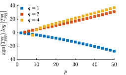
Figure 1: Magnitude (with sign) of the coefficients of the basis transformation $T_{pqq}^{qq}$ in Eq. 49a as a function of $p$ when $q=1$, $2$, and $4$.

Within the adopted Hermite-Laguerre gyro-moment method, the numerical evaluation of the collision operators leads to the calculation of large sums of algebraic coefficients such as the ones appearing, for example, in sec. 3.1.2. In the numerical implementation of the gyrokinetic pseudo-spectral method proposed by (Mandell et al., 2018) where a GK Dougherty collision operator is considered, a closed analytical formula is used for the lowest order coefficients from the products between Laguerre polynomials (such as $d_{hs_{1}}^{0}$ and $\overline{d}_{0kf}^{0}$ defined in Eqs. 54 and 62 respectively). On the other hand, a Fourier dealiased scheme is employed to numerically compute the integral representation of the higher order coefficients. This method can be generalized to obtain $\overline{d}_{nkf}^{m}$ and $d_{n^{\prime}hs_{1}}^{m}$, but it is unpractical for the basis transformation coefficients $T^{lk}_{pjm}$ that appear in the operators considered here. This is because of the rapid increase in magnitude of these coefficients and the enhancement of the oscillatory nature of the basis functions (such as the Hermite polynomials) with the order of the polynomials basis. In fact, due to the presence of positive and negative numerical coefficients of different magnitude that eventually cancel each other, the Hermite-Laguerre formulation of the present collision models is highly sensitive to round off errors. This becomes particularly pronounced as the order of the polynomials basis increases. As an example, Fig. 1 displays the magnitude (with sign) of a few of the basis transformation coefficients, in particular $T_{pqq}^{qq}$ defined in Eq. 49a. An increase of $40$ orders is observed by going from $p=1$ to polynomials of order $p=50$. We note that similar issues are observed in the numerical implementation of spectral methods based on generalized Laguerre polynomials in the energy variable $v^{2}$ (Belli & Candy, 2011). In addition, it should be mentioned that convergence tends to be relatively slow when using Laguerre polynomials in $v^{2}$ because they have very similar shapes for the bulk of the distribution (Landreman & Ernst, 2013). As a matter of fact, we find that the use of double and/or quadruple precision is not sufficient to carry out the evaluation of the coefficients required for the Coulomb and Sugama operators.

To avoid spurious unphysical effects associated to precision loss in the linearized collision operators, we evaluate the closed analytical expressions of the numerical coefficients and perform the sums numerically using a multiple precision arithmetic package. To avoid redundancy, the species-independent numerical coefficients that depend on the mass and temperature ratios of the colliding species ($\overline{\nu}_{*ab}^{Tpjt}$, $\overline{\nu}_{*ab}^{Fpjt}$ and $\overline{\nu}_{*ab}^{Spjd}$ defined in Appendices A and B) are computed once and stored. Then, given the normalized perpendicular wavenumber $b_{a}$, the mass and temperature ratios, the GK linearized collision operators can be obtained by performing linear combinations of the previously computed numerical coefficients.

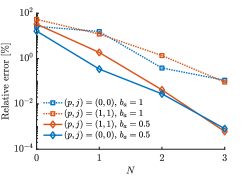
Figure 2: Relative error of the diagonal elements, (blue lines) $(p,j)=(0,0)$ and (orange lines) $(p,j)=(1,1)$, of the GK Coulomb [see Fig. 3], when (solid) $b_{a}=0.5$ and (dotted) $b_{a}=1$, as a function of $N$. The relative error is measured with respect to the $N=4$.

Because of FLR effects, infinite sums arise in the GK Coulomb and Sugama operators from the expansion of the Bessel functions, $J_{m}$, in terms of associated Laguerre [see Eq. 12]. These sums appear in the Hermite-Laguerre projections, such as the ones in sec. 3.1.2 and Eq. 106. For their numerical implementations, we truncate these sums at a finite $N>0$. While a large number of terms in the FLR terms might a priori be needed for a good convergence, the nature of the kernel function, $\mathcal{K}_{n}$ defined in Eq. 13, ensures that only a small number of terms contribute in the sums at a given perpendicular wavenumber. This is because the kernel functions $\mathcal{K}_{n}$ decreases rapidly with $n$, as $\mathcal{K}_{n}\sim 1/n!$ for large $n$ for all $b_{a}$, and $\mathcal{K}_{n}\sim b_{a}^{2n}/n!$ when $b_{a}\ll 1$ (Frei et al., 2020). Additionally, since the maximum of $\mathcal{K}_{n}$ occurs at $b_{a}=2\sqrt{n}$, as a rule of thumb, one can choose $N$ such that $N>b_{a}^{2}/4$. Figure 2 displays the relative error of the diagonals elements of the GK Coulomb operator corresponding to the gyro-moments (blue lines) $(p,j)=(0,0)$ and (orange lines) $(p,j)=(1,1)$, for typical values of the normalized perpendicular wavenumber in the ion gyroscale when (solid lines) $b_{a}=0.5$ and (dotted lines) $b_{a}=1$, as a function of $N$. The relative error is computed with respect to the $N=4$ case. As observed, the error decreases linearly with $N$, and it is of the order of $\lesssim 0.1\%$ or smaller at $N=3$, when $b_{a}=1$. A similar behaviour is found with the GK Sugama operator.

Finally, we discuss the coupling between gyro-moments introduced by the GK Coulomb collision operator. By mapping the gyro-moments into a one dimensional array, the GK Coulomb operator can be represented in matrix form, relating the projection of the collision operator with the gyro-moments. Given $(P_{a},J_{a})<\infty$, we can construct the collisional matrix by defining the one dimensional gyro-moment array as $[N_{a}^{00},N_{a}^{01},N_{a}^{02},\dots,N_{a}^{0J},N_{a}^{10},N_{a}^{11},N_{a}^{12},\dots,N_{a}^{P_{a}0},\dots,N_{a}^{P_{a}J_{a}}]^{T}$ and the one dimensional index $\bar{l}(p,j)=(J_{a}+1)p+1+j$. Figure 3 displays the block matrix obtained from the GK Coulomb collision operator for like-species when $b_{a}=0.5$ for $(p,j)\leq(P_{a},J_{a})$. It is visible that, the $p$th Hermite blocks is coupled with the $l=p+2n$ block (with $n$ a positive integer). We remark that the block structure of the matrix representing the Coulomb collision operator results from the vanishing basis transformation coefficients $T^{lk}_{pjm}$. Notice also the negative elements in the diagonal with a magnitude that increases with $\bar{l}$ at fixed $p$, yielding damping of higher order gyro-moments. A similar block matrix is obtained for the GK Sugama.

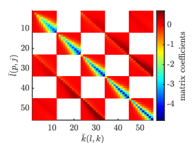
Figure 3: Block matrix obtained from the GK Coulomb collision operator for like-species when $b_{a}=0.5$. We show, on the vertical axis, the one-dimensional index $\bar{l}(p,j)=(J_{a}+1)p+1+j$ and, on the horizontal axis, the one-dimensional index $\bar{k}(l,k)=(J_{a}+1)l+1+k$.

5 Numerical Tests

This section presents the numerical tests and benchmarks of the implementation of the GK Coulomb and Sugama collision operators. First, we numerically investigate the linear growth rate of the ion-temperature gradient (ITG) instability in Sec. 5.1. For this test, we consider both the linearized GK Coulomb and Sugama collision operators and various perpendicular wavenumbers and levels of collisionality. As a second test, in Sec. 5.2, we address the collisional damping of zonal flows (ZF). We benchmark our results against the DK linearized Coulomb and GK Sugama collision operators (Crandall et al., 2020) currently available in the public release of the gyrokinetic continuum code GENE (Jenko et al., 2000), finding good agreement.

5.1 Ion-Temperature Gradient Instability

Belonging to the class of ion-gyroscale gradient-driven drift-wave instability, the ion temperature gradient (ITG) mode is widely recognised as the main candidate to explain the level of anomalous ion heat transport observed experimentally in the tokamak core (Garbet et al., 2004). As a matter of fact, the collisionless theory of ITG mode in core conditions is well established and documented (see, e.g, Romanelli, 1989; Hahm & Tang, 1989; Romanelli & Briguglio, 1990; Chen et al., 1991). On the other hand, the role of the ITG mode is less clear in the edge and in the SOL region due to the limitation of Braginskii-like fluid models that are most often applied in these regions (Hallatschek & Zeiler, 2000; Mosetto et al., 2015). While a complete collisional theory of ITG modes using the gyro-moment approach will be subject of a future publication, we consider here the slab growth rate of this mode, as a function of the collisionality and the perpendicular wavenumber, when the GK Coulomb and Sugama collision operators are used. We also perform a comparison with GENE.

We focus on a shearless slab configuration and measure the relative strength of the ion temperature and density gradients by the dimensionless parameter $\eta=L_{N}/L_{T_{i}}$, where $L_{N}=\left|\gradient_{\perp}\ln N\right|^{-1}$ and $L_{T_{i}}=\left|\gradient_{\perp}\ln T_{i}\right|^{-1}$. We assume that the electrons are adiabatic, and consider only like-species collisions, $C_{i}=C_{ii}$, neglecting the ion-electron collisions since they occur on a time scale larger by a factor $O(\sqrt{m_{i}/m_{e}})$ than the ion-ion collisions. We neglect magnetic gradient drifts and particle trapping, considering therefore the slab ITG branch. We define the normalized ion-ion collisionality by the parameter $\nu=L_{N}\nu_{ii}/c_{s}$, with $c_{s}^{2}=T_{e}/m_{i}$ the ion sound speed, and we impose $T_{e}=T_{i}$. We normalize the perpendicular wavenumber, $k_{\perp}$, to $\rho_{s}=c_{s}/\Omega_{i}$ and the linear growth rate $\gamma$ to $c_{s}/L_{N}$. The parallel wavenumber is fixed at $k_{\parallel}=0.1/L_{N}$. We solve the gyro-moment hierarchy, in Section 2, with $(P,J)=(20,8)$ for the ion species by applying a closure by truncation such that $N_{i}^{pj}=0$ for $(p,j)>(P,J)$. We have carefully checked that the considered number of ion gyro-moments provide a sufficient resolution of the velocity space for the numerical tests carried out in this section. We note the slab ITG mode relies mainly on parallel dynamics and thus emphasizes the faster convergence of the Hermite expansion in $v_{\parallel}$ relative to the Laguerre expansion.

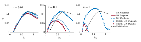
Figure 4: Comparisons between the GK Coulomb (solid blue lines) and GK Sugama (solid red lines) operator models, given in Eq. 72 and Eqs. 98 and 112, and GENE (markers), as a function of the perpendicular wavenumber, $k_{\perp}$ for different collisionalities. The collisionless solution (dotted lines) is shown for comparison. A good agreement is found with the GENE operators. Here, $\eta=3$.

The numerical results are shown in Fig. 4. We consider the full linearized GK Coulomb collision operator given in Eq. 64, and the GK Sugama collision operator, with test and field components defined in Eqs. 98 and 112, respectively. The temperature gradient strength is fixed at $\eta=3$, and a scan in the perpendicular wavenumber $k_{\perp}$ is performed at different collisionalities. The GK Coulomb is represented by the solid blue lines, and the GK Sugama by the red solid lines, while their DK limits are shown for comparison by the dashed lines. Markers represent GENE results with the DK Coulomb and GK Sugama. First of all, we note that a good agreement is found between our results and GENE. We have also successfully compared the DK Sugama operator model with GENE (comparison not shown). This shows the ability of the gyro-moment approach to accurately describe FLR collisional damping in advanced GK collision operators. From a more physical perspective, we observe that the GK Sugama yields an underestimate of the ITG growth rate (of the order of $15\%$ or less) compared to GK Coulomb for wavelengths smaller than the one corresponding to the peak growth rate. We also note, by comparing the DK operators, that FLR collisional effects provide a strong damping and that the DK Sugama follows closely the DK Coulomb, similar to results obtained for TEMs (Pan et al., 2020, 2021). In principle, comparison with the GK Coulomb operator in GENE (Pan et al., 2020) is also possible when it becomes publicly available.

To conclude our analysis of the ITG mode, we illustrate the effect of the collisional polarization terms in the GK Coulomb collision operator, expressed by $\sum_{i=1}^{2}(\mathcal{C}^{Tlk}_{ab\phi i}+\mathcal{C}^{Flk}_{ab\phi i})$ appearing in Eq. 67. We remark that $\mathcal{C}^{Tlk}_{aa\phi 1}+\mathcal{C}^{Flk}_{aa\phi 1}=0$ for like-species, such that only the $\mathcal{C}^{Tlk}_{aa\phi 2}$ and $\mathcal{C}^{Flk}_{aa\phi 2}$ terms in the polarization contribute in the GK linearized Coulomb operator. We perform a scan of the growth rate at a fixed collisionality ($\nu=0.1$), as a function of the perpendicular wavenumber $k_{\perp}$ for different temperature gradient strengths $\eta$. The results are shown in Fig. 5 where the growth rates with the GK Coulomb that include and exclude the polarization terms are shown by the solid black and red lines, respectively. It is observed that the collisional polarization terms have a negligible effect on the ITG peak growth rate. On the other hand, the difference increases up to $15\%$ for short wavelengths.

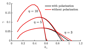
Figure 5: Effects of polarization given in Eq. 67 in the GK Coulomb collision operator on the ITG growth rate for different temperature gradients as the function of the perpendicular wavenumber $k_{\perp}$ when $\nu=0.1$.

5.2 Collisional Damping of Zonal Flow

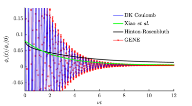
Figure 6: Collisional ZF damping using (blue solid line) the DK Coulomb collision operator given in Eq. 72 and (red solid with markers) the GENE results. The Hinton-Rosenbluth collisional damping, Eq. 125, is shown by the black line, and the collisional damping predicted by Xiao et al. (2007), given in Eq. 126, is plotted by the solid green. A good agreement is found between GENE results and gyro-moment approach. Here, the parameters are $k_{r}=0.05$, $\epsilon=0.1$, $q=1.4$ and $\nu_{i*}=3.1$.

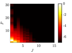
Figure 7: Modulus of the normalized Hermite-Laguerre spectrum of the zonal flow residual at $\nu t=10$ taken from Fig. 6 on a logarithmic scale.

Zonal flows (ZF) can reduce the particle and heat exhaust from the core in magnetised plasma confinement devices (Hasegawa et al., 1979; Hammett et al., 1993). These self-generated, primarily poloidal and axisymmetric, flows help to shear apart structures that propagate radially, caused by the growth of an instability driven by, e.g., a steep pressure gradient. In fact, ZF regulate and, ultimately, can suppress the turbulent transports driven by, e.g., ITG and trapped electron modes (Candy & Waltz, 2003; Ernst et al., 2004).

The collisionless damping of self-generated ZF driven by ITG turbulence to a non vanishing residual in the large radial wavelength limit has been addressed and calculated by Rosenbluth & Hinton (1998), in a seminal work that considers a large aspect ratio and circular flux surface geometry. Later, including the effects of ion collisions modelled by a pitch angle scattering operator, Hinton & Rosenbluth (1999) showed that the ZF component of the electrostatic potential, $\phi_{z}(t)$, decays to a smaller values than the one predicted by the collisionless theory on long time scales. Hinton-Rosenbluth’s analytical prediction,

$$\frac{\phi_{z}(t)}{\phi_{z}(0)}=\varpi\exp\left(\varpi^{2}\alpha^{2}t\right)\left[1-\text{erf}\left(\varpi\alpha t^{1/2}\right)\right],$$ (125)

has been the subject of numerous tests and benchmarks of gyrokinetic codes (see, e.g., Idomura et al., 2008; Merlo et al., 2016). In Eq. 125, we introduce $\varpi=1/(1+1.61q^{2}/\sqrt{\epsilon})$ and $\alpha=3\pi q^{2}\bar{\nu}^{1/2}/(\epsilon\Lambda^{3/2})$, where $\Lambda\simeq\ln[16(\epsilon/\bar{\nu}t)^{1/2}]$ and $\bar{\nu}=0.61\nu_{ii}$. In addition, $\epsilon$ is the local inverse aspect ratio and $q$ is the safety factor. As an extension of the work by Hinton & Rosenbluth (1999) to arbitrary collisionality, Xiao et al. (2007) retains the velocity dependence of the deflection frequency, $\nu_{ii}^{D}(v)$, appearing in the pitch angle scattering operator, as well as a momentum restoring field component, in the limit of ZF with perpendicular wavelength larger than the ion poloidal Larmor radius. In fact, Xiao et al. (2007) shows that the time dependence of the collisional decay of the ZF residual is predicted by

$$\frac{\phi_{z}(t)}{\phi_{z}(0)}=\frac{\beta}{1+\beta}\left[1+\frac{1-\Theta}{\Theta+\beta}e^{-(1+\beta)\Gamma\nu_{ii}t/[\Theta+\beta]}\right],$$ (126)

with $\beta=\epsilon^{2}/q^{2}$, $\Theta=1.635\epsilon^{3/2}+\epsilon^{2}/2+0.360\epsilon^{5/2}$ and $\Gamma=0.4(1.46\sqrt{\epsilon}+1.32\epsilon)$. Since the pitch angle scattering is the dominant collisional damping process in large aspect ratio tokamak (Hinton & Rosenbluth, 1999), energy diffusion - neglected in Eq. 126 - is expected to play a subdominant role. Equation 126 provides an accurate analytical estimate to benchmark the ZF collisional damping using the DK Coulomb and DK Sugama collision operators.

As a test of the implementation of the collisional gyro-moment hierarchy, given in Section 2, we consider a shearless, toroidal circular concentric flux surface geometry, with an initial zonal density perturbation radially varying with a wavevector $\bm{k}=k_{r}\gradient r$. Density and temperature equilibrium gradients are neglected. A finite number of ion gyro-moments, $(P,J)=(30,15)$, are evolved and electrons are assumed adiabatic. We consider a level of ion-ion neoclassical collisionality that is in the Pfirsch-Schluter regime, i.e. $\nu_{i*}\simeq 3.1$. In this parameter regime, collisions smear out fine structures in $v_{\parallel}$, which develop at low collsionality because of passing ions and finite orbit width effects and might require a larger number of gyro-moments (Idomura et al., 2008).

Figure 6 shows the ZF collisional damping predicted by the gyro-moment approach (blue solid line) using the DK Coulomb collision operator and its comparison with GENE results (red line with cross markers). We also plot Hinton and Rosenbluth’s, Eq. 125, and Xiao’s, Eq. 126, predictions. An excellent match is observed between the gyro-moment approach and GENE simulation. In addition, the collisional ZF damping agrees with the analytical prediction, given in Eq. 126. Ultimately, the Hermite-Laguerre spectrum at $t=10/\nu_{ii}$, in Fig. 7, reveals that the velocity space dependence of the ion distribution function is well resolved. We remark that the decay of the spectrum is slower along the Hermite direction compared to the Laguerre direction. This is primarily because of the the ballistic mode response of the passing ion population (Idomura et al., 2008).

We now focus on the collisional ZF damping when the linearized GK Coulomb and GK Sugama collision operators are considered. The results are shown in Fig. 8, for $k_{r}=0.1$ (left) and $k_{r}=0.5$ (right). The ZF damping by the GK Sugama operator is compared with GENE. Other parameters are the same as in Fig. 6. The GK Coulomb collision operator yields a smaller collisional damping of the ZF residual than the one predicted by the GK Sugama. The same qualitative result was obtained in (Pan et al., 2020, 2021), but in the low collisionality banana regime. We remark that the GK Sugama agrees well with GENE simulations. The observed difference between GK Coulomb and Sugama operators in the ZF residual collisional damping suggests that higher ion particle and heat fluxes can be expected in nonlinear simulations that use the GK Sugama operator rather than the GK Coulomb, particularly in the $\nu_{i*}\gtrsim 1$ Pfirsch-Schlüter regime. However, the opposite trend in TEM turbulence was observed in Pan et al. (2021).

Furthermore, we note that larger oscillations in the gyro-moment approach are observed compared to GENE when $k_{r}$ increases. This is related to the large number of gyro-moments required to accurately resolve the resonant passing particle dynamics and finite orbit width effects during the geodesic mode oscillation. The low resolution does not influence the collisional damping of the ZF residual.

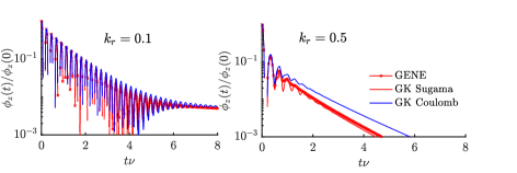
Figure 8: Collisional ZF damping using (blue solid line) the GK Coulomb collision operator, given in Eq. 64, (red solid) the GK Sugama, given in Eq. 98, and (red solid with markers) GENE when (left) $k_{r}=0.1$ and (right) $k_{r}=0.5$. Others parameters are the same in as Fig. 6.

6 Convergence Test

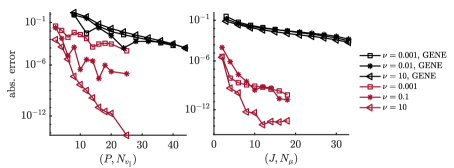
Figure 9: Absolute error of the ITG linear growth rate as a function of the number of gyro-moments, $(P,J)$ (red), and the number of velocity-space grid points, $(N_{v_{\parallel}},N_{\mu})$ used in GENE (black), for increasing collisionality regimes. We display, on the same horizontal axis, the gyro-moment and GENE errors as a function of the discretization along the parallel direction given by $P$ for the gyro-moment method and $N_{v_{\parallel}}$ for GENE (left panel), and as a function of the discretization along the perpendicular direction given by $J$ for the gyro-moment method and $N_{\mu}$ for GENE (right panel), respectively. Collisions are modelled by the DK Coulomb operator. Here, $k_{\perp}=0.5$, $k_{\parallel}=0.1$ and $\eta=3$.

The numerical tests in Section 5 illustrate the ability of the gyro-moment approach to model collisional effects using advanced linearized GK collision operators. Additionally, the direct comparisons with the GK continuum GENE code show that the Hermite-Laguerre approach is able to resolve the velocity dependence of the distribution functions in the presence of collisions, as shown in Fig. 7, with a finite number of gyro-moments even when a simple closure by truncation is adopted.

As we now show, the number of gyro-moments necessary to describe the distribution function decreases with the collisionality, as collisions provide a natural way to smear out any sharp velocity space structures and damp the higher order gyro-moments in the Hermite-Laguerre spectrum. Thus, in the high collisional regime, only the lowest order gyro-moments are necessary, while, as the collisionality decreases, a larger number of gyro-moments is necessary to resolve the essential kinetic effects in order to retrieve the collisionless solution [see, e.g., dotted black line in Fig. 4]. We remark that the presence of kinetic effects related to, e.g., finite magnetic gradient drifts, passing ions, particle trapping and finite orbit width can highly affect the velocity space structures, and ultimately deteriorates the convergence of the Hermite-Laguerre spectrum, when collisions are subdominant. These fine scale structures require a fine velocity space resolution.

Contrary to velocity space grid methods, the Hermite-Laguerre gyro-moment approach features a spectral convergence rate. This convergence rate is faster than any algebraic schemes that characterize the grid methods (Boyd, 2001), though some basis functions converge faster than others, depending on the velocity space structure present in the distribution function (Landreman & Ernst, 2013). To illustrate the convergence properties of the gyro-moment method, we compute the absolute error on the ITG growth rate as a function of the ion Hermite-Laguerre resolution $(P,J)$. Similarly, by using GENE, we consider convergence study with the number of velocity-space grid points, defined by $N_{v_{\parallel}}$ and $N_{\mu}$ (with $N_{v_{\parallel}}$ the number of grid points in the parallel velocity space direction $v_{\parallel}$, and $N_{\mu}$ the number of grid points in the perpendicular velocity space direction $\mu$) for different collisionality using the DK Coulomb collision operator. We first note that the difference between the most resolved growth rate evaluated by GENE and by the gyro-moment method is less than $3\%$ in all cases. The results are shown in Fig. 9 ($k_{\perp}=0.5$, $k_{\parallel}=0.1$ and $\eta=3$). The convergence with respect to the parallel and perpendicular velocity direction refinement are plotted on the left and on the right panel, respectively.

As observed in Fig. 9, the gyro-moment approach features a convergence rate in both velocity-space directions that is sensitive to the collisionality $\nu$ (as discussed above), while the velocity-space grid method, used in GENE, shows a convergence rate that is much less sensitive to $\nu$. In fact, while in both methods, fewer number of gyro-moments and grid points in velocity-space is required in the high collisional regime as the perturbed distribution function does not feature sharp velocity-space structures, the effect of collision is much stronger on the number of gyro-moments required than on grid points. While the increase of the convergence rate of the gyro-moment method with $\nu$ is clearly visible in Fig. 9, we notice that the GENE error also decreases with the collisionality $\nu$, but is much less visible. We remark that, in the case of slab ITG mode, the perturbed distribution function does not feature sharp velocity-space structures which appear, e.g., in the ballistic mode response from passing particles and in the trapping of particles in velocity-space (Idomura et al., 2008). However, preliminary studies show that the same conclusion on the convergence rate of the gyro-moment approach can be made even if stronger kinetic drives are present. Thus, the convergence study we carried out suggest that the gyro-moment approach offers a particularly efficient numerical scheme to simulate the plasma boundary, where the collisionality is larger (with respect to the strength of velocity space structure drive) than in the core, compared to a finite difference. A careful analysis of the description of fine velocity-space structure using the gyro-moment approach will be subject of a future publication.

7 Conclusion

In this work, we report on the derivation and numerical implementation of a linearized version of a full-F nonlinear gyrokinetic Coulomb collision operator (Jorge et al., 2019) based on an Hermite-Laguerre moment decomposition of the perturbed gyrocenter distribution function. Thanks to a spherical harmonic moment expansion technique, the gyro-average of the linearized Coulomb collision operator is analytically evaluated, projected onto the Hermite-Laguerre basis, and ultimately expressed in terms of gyro-moments. The obtained linearized gyrokinetic Coulomb collision operator is valid at arbitrary perpendicular wavenumber, and at arbitrary mass and temperature ratios of the colliding species. Within the same formalism, we have projected the linearized gyrokinetic Sugama collision operator (Sugama et al., 2009) onto the same basis. Additionally, neglecting the finite Larmor radius effects, the DK Coulomb and DK Sugama collision operators are deduced. One of the main advantages of the Hermite-Laguerre decomposition coupled with a basis transformation is that velocity integrals in the linearized GK collision operator models can be evaluated analytically, while a numerical approach is needed in continuum gyrokinetic codes (Crandall et al., 2020; Pan et al., 2020). It follows that the collision operators are expressed as linear combinations of gyro-moments, where the coefficients are only functions of perpendicular wavenumber, mass and temperature ratios. These coefficients can be evaluated numerically thanks to closed analytical formulas.

The implementation of the collision operator is described and numerical tests focused on the ITG growth rates and collisional ZF damping are reported. In particular, we show that the collisional damping of the ZF residual, predicted by the GK Sugama operator, is larger than the one obtained using the GK Coulomb operator. This points out that, since ZF residual plays an important role in the self-regulation of turbulent transport, the choice of collision operator might affect the predicitions of the nonlinear level of particle and heat fluxes. Additionally, the gyro-moment approach is tested and benchmarked, for the first time, against the continuum gyrokinetic code GENE (Jenko et al., 2000), reporting an excellent agreements between the DK Coulomb and GK Sugama operator. The comparisons between spectral and velocity space grid approach to collisional gyrokinetic modelling illustrate the main advantage of the Hermite-Laguerre approach, i.e. its ability to reduce the number of required gyro-moments, as the plasma collisionality increases. This hints that the gyro-moment formulation provides an ideal framework for the development of a multi-fidelity scheme to simulate the turbulent plasma dynamics in the boundary region of tokamak devices where collisions play an important role and cannot be ignored (Frei et al., 2020).

Finally, we remark that the Hermite-Laguerre expansion presented here can be easily applied to other gyrokinetic collision operators, such as the improved GK Sugama operator (Sugama et al., 2019). Ultimately, it allows for comparisons between collision operator models over a wide range of physical phenomena.

8 Acknowledgement

The authors acknowledge helpful discussions with S. Brunner and P. Donnel. The authors thank the anonymous reviewers whose suggestions helped improve and clarify this work. The simulations presented herein were carried out in part at the Swiss National Supercomputing Center (CSCS) under the project ID s882 and in part on the CINECA Marconi supercomputer under the GBSedge project. This research was supported in part by the Swiss National Science Foundation, and has been carried out within the framework of the EUROfusion Consortium and has received funding from the Euratom research and training programme 2014 - 2018 and 2019 - 2020 under grant agreement No 633053. The views and opinions expressed herein do not necessarily reflect those of the European Commission.

9 Declaration of Interests

The authors report no conflict of interest.

Appendix A Coulomb Speed Functions

We report the analytical expressions of the speed functions, $\nu_{ab}^{Tpj}$ and $\nu_{ab}^{Fpj}$, appearing in Eq. 34a. The speed function $\nu_{ab}^{Tpj}$ associated with the test component of the Coulomb operator is given by

$$\nu_{ab}^{Tpj}=\sum_{l=0}^{j}L_{jl}^{p}\nu_{*ab}^{Tpjl}$$ (127)

with

$$\nu_{*ab}^{Tpjl}=\chi\nu_{ab}s_{a}^{2l+p}\sum_{n=0}^{2}\left[\frac{\erf(s_{b})}{s_{b}}\frac{a^{pl}_{abn}}{s_{a}^{2n}}+\erf^{\prime}(s_{b})\frac{a_{abn}^{{}^{\prime}pl}}{s_{a}^{2n}}\right],$$ (128)

where we introduce the coefficients

$$a_{ab0}^{pl} =-\frac{4\sigma(\tau-1)}{\tau},$$ (129a)

$$a^{pl}_{ab1} =4\frac{\sigma}{\tau}l(\tau-2)-p(p-2\sigma+\frac{4\sigma}{\tau}+1),$$ (129b)

$$a_{ab2}^{pl} =\frac{\sigma}{\tau}\left[4l^{2}+4l(p-1)+\frac{3}{2}p(p-1)\right],$$ (129c)

$$a^{{}^{\prime}pl}_{ab0} =\frac{4(\tau-1)(\sigma+\tau)}{\tau},$$ (129d)

$$a^{{}^{\prime}pl}_{ab1} =-2(p+2l)\left[\frac{\sigma}{\tau}(\tau-2)-1\right],$$ (129e)

$$a_{ab2}^{{}^{\prime}pl} =-\frac{\sigma}{\tau}\left[4l^{2}+4l(p-1)+\frac{3}{2}p(p-1)\right],$$ (129f)

with $\sigma=m_{a}/m_{b}$, $\tau=T_{a}/T_{b}$, and $\chi=v_{Ta}/v_{Tb}=\sqrt{\tau/\sigma}$. Using Eq. 128, a closed analytical expression for

$$\overline{\nu}_{*ab}^{Tpjd}=\int d\bm{v}s_{a}^{p+2d}\nu_{ab}^{Tpj}F_{Ma}$$ (130)

can be derived. Performing the integral over the speed $v$ variable, one obtains

$$\overline{\nu}_{*ab}^{Tpjd}=\sum_{j_{1}=0}^{j}L_{jj_{1}}^{p}\sum_{n=0}^{2}\left[a_{abn}^{pj_{1}}\alpha_{Eab}^{dj_{1}np}+a_{abn}^{{}^{\prime}pj_{1}}\alpha_{eab}^{dj_{1}np}\right],$$ (131)

where we introduce the quantities

$$\alpha_{Eab}^{dj_{1}np} =\frac{4\nu_{ab}}{\sqrt{\pi}}E_{ab}^{d+j_{1}+p-n},$$ (132)

$$\alpha_{eab}^{dj_{1}np} =\frac{4\chi\nu_{ab}}{\sqrt{\pi}}e_{ab}^{d+j_{1}+p-n+1},$$ (133)

with

$$e_{ab}^{k} =\int_{0}^{\infty}ds_{a}s_{a}^{2k}\erf^{\prime}(s_{b})e^{-s_{a}^{2}}=\frac{(k-1/2)!}{(-1/2)!(1+\chi^{2})^{k+1/2}},$$ (134a)

$$E_{ab}^{k} =\int_{0}^{\infty}ds_{a}s_{a}^{2k+1}\erf(s_{b})e^{-s_{a}^{2}}=\frac{\chi}{2}\sum_{j=0}^{k}\frac{k!}{j!}e_{ab}^{j}.$$ (134b)

The speed function $\nu_{ab}^{Fpj}$ associated with the field component of the Coulomb operator is given by

$$\nu_{ab}^{Fpj}=\sum_{l=0}^{j}L_{jl}^{p}\nu_{*ab}^{Fpjl},$$ (135)

with

$$\nu_{*ab}^{Fpjl} =\frac{\nu_{ab}}{\chi}\sum_{n=0}^{1}\left[s_{b}^{p+2(l+n)}b_{abn}^{{}^{\prime}pl}\erf^{\prime}(s_{b})+I_{+}^{2l+1}s_{b}^{p+2n}b_{+abn}^{pl}+b_{-abn}^{pl}\frac{I_{-}^{2(p+l+1)}}{s_{b}^{p+1-2n}}\right],$$ (136)

where

$$b_{ab0}^{{}^{\prime}pl} =4\frac{\tau^{2}}{\sigma},$$ (137a)

$$b_{ab1}^{{}^{\prime}pl} =-8\frac{(p^{2}+p-1)}{(2p-1)(2p+3)},$$ (137b)

$$b_{+ab0}^{pl} =-8\frac{p(p-1)(l+1)}{(2p+1)(2p-1)}-\frac{\tau 8(1+p-\sigma p)}{\sigma(2p+1)},$$ (137c)

$$b_{+ab1}^{pl} =\frac{8(p+1)(p+2)}{(2p+1)(2p+3)},$$ (137d)

$$b_{-ab0}^{pl} =\frac{4(p+1)(p+2)(2p+2l+3)}{(2p+1)(2p+3)}+\frac{8\chi^{2}(p-\sigma p-\sigma)}{(2p+1)},$$ (137e)

$$b_{-ab1}^{pl} =-8\frac{p(p-1)}{(2p+1)(2p-1)}.$$ (137f)

Using Eq. 136, a closed analytical expression for

$$\overline{\nu}_{*ab}^{Fpjd}=\int d\bm{v}s_{a}^{p+2d}\nu_{ab}^{Fpj}F_{Ma},$$ (138)

can be obtained by performing the integral over the speed variable $s_{a}$, yielding

$$\overline{\nu}_{*ab}^{Fpjd}=\sum_{j_{1}=0}^{j}L_{jj_{1}}^{p}\sum_{n=0}^{1}\left[b_{abn}^{{}^{\prime}pj_{1}}\beta_{eab}^{pdnj_{1}}+b_{+abn}^{pj_{1}}\beta_{+eab}^{pdnj_{1}}+b_{-abn}^{pj_{1}}\beta_{-Eeab}^{pdnj_{1}}\right],$$ (139)

where we introduce

$$\beta_{eab}^{pdnj_{1}} =\frac{4\nu_{ab}}{\sqrt{\pi}}\chi^{p+2j_{1}+2n-1}e_{ab}^{p+1+d+j_{1}+n},$$ (140)

$$\beta_{+eab}^{pdnj_{1}} =\frac{4\nu_{ab}}{\sqrt{\pi}}\chi^{p+2n-1}\sum_{j_{2}=0}^{j_{1}}\frac{\chi^{2j_{2}}j_{1}!}{j_{2}!}\frac{e_{ab}^{p+n+1+d+j_{2}}}{2},$$ (141)

$$\beta_{-Eeab}^{pdnj_{1}} =\frac{4\nu_{ab}}{\sqrt{\pi}}\chi^{2n-p-2}\left[\frac{(p+j_{1}+1/2)!}{(1/2)!}\frac{E_{ab}^{d+n}}{2}\right.$$

$$\left.-\sum_{j_{2}=0}^{p+j_{1}}\frac{\chi^{2j_{2}+1}(p+j_{1}+1/2)!}{(j_{2}+1/2)!}\frac{e_{ab}^{d+n+j_{2}+1}}{2}\right].$$ (142)

Appendix B Hermite-Laguerre Expansion of $C_{ab}^{S}$ and $R^{\perp}_{ab}$

We report the details of the Hermite-Laguerre expansion of $C_{ab}^{S}$, $R^{\perp}_{ab}$, $\mathcal{C}_{ab}^{Slk}$ and $R^{\perp lk}_{ab}$ given in Eqs. 99 and 100, that appear in the test component of the linearized gyrokinetic Sugama operator, Eq. 98. The derivation below can be used as an example to derive the Hermite-Laguerre expansions of the remaining terms in the GK Sugama collision operator given in Eq. 105 and Eq. 113.

In order to obtain the gyro-moment expansion of $C_{ab}^{S}$ given in Eq. 76, we first expand $h_{a}$ as

$$h_{a}=\sum_{p=0}^{\infty}\sum_{j=0}^{\infty}\frac{F_{Ma}c_{p}}{\sigma_{j}^{p}}\mathcal{H}_{a}^{pj}s_{a}^{p}P_{p}(\xi)L_{j}^{p+1/2}(s_{a}^{2}),$$ (143)

with $c_{p}=\sqrt{\pi^{1/2}p!/[2^{p}(p-1/2)!]}$, and $\mathcal{H}_{a}^{pj}$ defined by

$$\mathcal{H}_{a}^{pj}=c_{p}\int d\bm{v}h_{a}s_{a}^{p}P_{p}(\xi)L_{j}^{p+1/2}(s_{s}^{2}).$$ (144)

Using the basis transformation, Eq. 49 with $m=0$, the coefficients $H_{a}^{pj}$ are related to the nonadiabatic moments $n_{a}^{lk}$ by

$$\mathcal{H}_{a}^{pj}=c_{p}\sum_{g=0}^{p+2j}\sum_{h=0}^{j+\lfloor p/2\rfloor}T_{pj}^{gh}\sqrt{2^{g}g!}n_{a}^{gh}.$$ (145)

We remark that $c_{p}s_{a}^{p}P_{p}(\xi)=\left<\mathsfbi{Y}^{p}\right>_{\bm{R}}\cdot\bm{\bm{e}}^{p0}$ (or equivalently $\left<\mathsfbi{Y}^{p}\right>_{\bm{r}}\cdot\bm{\bm{e}}^{p0}$, as the spatial dependence of $\mathsfbi{Y}^{p}$ on $\bm{s}_{a}=\bm{v}/v_{Ts}(\bm{R})$ is neglected), and is motivated by the fact that the velocity space derivatives, contained in Eq. 75, can be easily evaluated using the pitch angle and energy variables $(\xi,s_{a})$. In fact, inserting Eq. 143 into Eq. 75 and expanding the associated Laguerre polynomials in monomial basis thanks to Eq. 26 yield

$$C_{ab}^{S}(h_{a}) =\sum_{p,j}\frac{F_{aM}c_{p}}{\sigma^{p}_{j}}\mathcal{H}_{a}^{pj}P_{p}(\xi)\nu_{ab}^{Spj}(v),$$ (146)

where the speed dependent frequency, $\nu_{ab}^{Spj}(v)=\nu_{ab}^{\parallel pj}(v)-p(p+1)\nu_{ab}^{Dpj}(v)$, with

$$\nu_{ab}^{\parallel pj}(v) =\nu_{ab}\sum_{j_{1}=0}^{j}L_{jj_{1}}^{p}s_{a}^{p+2j_{1}}\sum_{n=0}^{1}\left[\erf(s_{b})s_{a}^{-(3+2n)}\alpha_{abe}^{pj_{1}n}+\erf^{\prime}(s_{b})\alpha_{abE}^{pj_{1}n}s_{a}^{-2(n+1)}\right],$$ (147)

with

$$\alpha_{abE}^{pj_{1}0} =-\frac{2\sigma}{\tau}(p+2j_{1}),$$ (148a)

$$\alpha_{abE}^{pj_{1}1} =\frac{\sigma}{\tau}(p+2j_{1})(2j_{1}+p-2),$$ (148b)

$$\alpha_{abe}^{pj_{1}0} =\frac{2}{\chi}(p+2j_{1})\left(1+\chi^{2}\right),$$ (148c)

$$\alpha_{abe}^{pj_{1}1} =\frac{1}{\chi}(p+2j_{1})\left(2-2j_{1}-p\right),$$ (148d)

and

$$\nu_{ab}^{Dpj}(v) =\nu_{ab}\sum_{j_{1}=0}^{j}L_{jj_{1}}^{p}s_{a}^{p+2j_{1}}\nu_{ab}^{D}(v),$$ (149)

Multiplying Eq. 146 by the Hermite-Laguerre basis, using the basis transformation in Eq. 49b with $m=0$, and performing the velocity integrals in the pitch angle coordinates yields

$$C_{ab}^{Slk}=\sum_{j=0}^{\infty}\sum_{p=0}^{l+2k}\sum_{h=0}^{k+\lfloor l/2\rfloor}\sum_{d=0}^{h}\frac{c_{p}}{\sigma_{p}^{j}}\frac{L_{hd}^{p}\left(T^{-1}\right)^{ph}_{lk}}{\sqrt{2^{l}l!}}\frac{1}{(2p+1)}\mathcal{H}_{a}^{pj}\overline{\nu}_{*ab}^{Spjd},$$ (150)

where the speed integrated frequency $\overline{\nu}_{*ab}^{Spjd}$ is defined by

$$\overline{\nu}_{*ab}^{Spjd} =\int d\bm{v}F_{aM}s_{a}^{p+2d}\nu_{ab}^{Spj}(v)$$

$$=\overline{\nu}_{*ab}^{\parallel pjd}-p(p+1)\overline{\nu}_{*ab}^{Dpjd},$$ (151)

with $\overline{\nu}_{*ab}^{Dpjd}=\int d\bm{v}F_{aM}s_{a}^{p+2d}\nu_{ab}^{Dpj}(v)$ and $\overline{\nu}_{*ab}^{\parallel pjd}=\int d\bm{v}F_{aM}s_{a}^{p+2d}\nu_{ab}^{\parallel pj}(v)$. We derive the closed analytical expressions of $\overline{\nu}_{*ab}^{Dpjd}$ and $\overline{\nu}_{*ab}^{\parallel pjd}$ using Eq. 134, yielding

$$\overline{\nu}_{*ab}^{Dpjd} =\frac{4\nu_{ab}}{\sqrt{\pi}}\sum_{j_{1}=0}^{j}L_{jj_{1}}^{p}\left[E_{ab}^{p+d+j_{1}-1}-\frac{1}{2\chi^{2}}E_{ab}^{p+d+j_{1}-2}+\frac{1}{2\chi}e_{ab}^{p+d+j_{1}-1}\right],$$ (152)

and

$$\overline{\nu}_{*ab}^{\parallel pjd}=\frac{4\nu_{ab}}{\sqrt{\pi}}\sum_{j_{1}=0}^{j}L_{jj_{1}}^{p}\sum_{n=0}^{1}\left[\alpha_{abE}^{pj_{1}n}E_{ab}^{p+d+j_{1}-n-1}+\alpha_{abe}^{pj_{1}n}e_{ab}^{p+d+j_{1}-n}\right],$$ (153)

respectively. Finally, expressing the coefficients $\mathcal{H}_{a}^{pj}$ appearing in Eq. 150 in terms of $n_{a}^{lk}$ thanks to Eq. 145, the gyro-moment expansion of $C_{ab}^{S}$, i.e. $\mathcal{C}_{ab}^{Slk}$ given in Eq. 99, is obtained.

We now aim to derive Eq. 100 defined by

$$R_{ab}^{\perp lk}=-\frac{k_{\perp}^{2}}{4\Omega_{a}^{2}}\int d\bm{v}\frac{H_{l}(s_{\parallel a})L_{k}(x_{a})}{\sqrt{2^{p}p!}}h_{a}\left[\nu_{ab}^{D}(v)\left(2v_{\parallel}^{2}+v_{\perp}^{2}\right)+\nu_{ab}^{\parallel}(v)v_{\perp}^{2}\right].$$ (154)

Because of the speed $(v)$ dependence of the deflection and energy diffusion frequencies, $\nu_{ab}^{D}(v)$ and $\nu_{ab}^{\parallel}(v)$ respectively, the velocity integral in Eq. 154 can be computed in pitch angle coordinates. To this aim, we use the Hermite-Laguerre expansion of the non-adiabatic part of the distribution function, $h_{a}$ [see Eq. 16], which can be written in terms of Legendre and associated Laguerre polynomials thanks to the basis transformation in Eq. 49b with $m=0$, such that

$$h_{a}=\sum_{p=0}^{\infty}\sum_{j=0}^{\infty}\sum_{r=0}^{p+2j}\sum_{s=0}^{j+\lfloor p/2\rfloor}F_{Ma}n_{a}^{pj}\frac{\left(T^{-1}\right)^{rs}_{pj}}{\sqrt{2^{p}p!}}s_{a}^{r}P_{r}(\xi)L_{s}^{r+1/2}(s_{a}^{2}).$$ (155)

Using again the same basis transformation in Eq. 154 with Eq. 155 yields

$$R_{ab}^{\perp lk} =-\frac{k_{\perp}^{2}}{4\Omega_{a}}\sum_{p=0}^{\infty}\sum_{j=0}^{\infty}\sum_{g=0}^{l+2k}\sum_{h=0}^{k+\lfloor l/2\rfloor}\sum_{r=0}^{p+2j}\sum_{s=0}^{j+\lfloor p/2\rfloor}\sum_{s_{1}=0}^{s}\sum_{h_{1}=0}^{h}L^{r}_{ss_{1}}L^{g}_{hh_{1}}\frac{\left(T^{-1}\right)^{gh}_{lk}}{\sqrt{2^{l}l!}}\frac{\left(T^{-1}\right)^{rs}_{pj}}{\sqrt{2^{p}p!}}N_{a}^{pj}$$

$$\times\frac{2}{\sqrt{\pi}}\int d\xi\int ds_{a}e^{-s_{a}^{2}}s_{a}^{r+g+4+2s_{1}+2h_{1}}P_{r}(\xi)P_{g}(\xi)$$

$$\times\left[\nu_{ab}^{D}(v)\left(\xi^{2}+1\right)+\nu_{ab}^{\parallel}(v)(1-\xi^{2})\right].$$ (156)

Finally, using the Legendre orthogonality relation and the identity given by respectively,

$$\int d\xi P_{g}(\xi)P_{r}(\xi)=\frac{2\delta_{g}^{r}}{2g+1},$$ (157)

$$\int d\xi P_{g}(\xi)P_{r}(\xi)\xi^{2}=d_{g}^{r},$$ (158)

with $d_{g}^{r}$ defined in Eq. 103, and introducing the speed integrated frequencies, $\overline{\nu}_{ab}^{\parallel k}=4\int_{0}^{\infty}ds_{a}s_{a}^{2k}\nu_{ab}^{\parallel}(v)e^{-s_{a}^{2}}/\sqrt{\pi}$ and $\overline{\nu}_{ab}^{Dk}=4\int ds_{a}e^{-s^{2}}s_{a}^{2k}\nu_{ab}^{D}(v)/\sqrt{\pi}$ with closed formulas found in Eq. 104, the Hermite-Laguerre expansion of $R_{ab}^{\perp}$, i.e. $R_{ab}^{\perp lk}$ is derived and is given in Eq. 100.

References

• Abel et al. (2008) Abel, I. G., Barnes, M., Cowley, S. C., Dorland, W. & Schekochihin, A. A. 2008 Linearized model Fokker-Planck collision operators for gyrokinetic simulations. i. theory. Physics of Plasmas 15 (12), 122509.
• Barnes et al. (2009) Barnes, M., Abel, I. G., Dorland, W., Ernst, D. R., Hammett, G. W., Ricci, P., Rogers, B. N., Schekochihin, A. A. & Tatsuno, T. 2009 Linearized model Fokker–Planck collision operators for gyrokinetic simulations. ii. numerical implementation and tests. Physics of Plasmas 16 (7), 072107.
• Belli & Candy (2011) Belli, E. A. & Candy, J. 2011 Full linearized Fokker–Planck collisions in neoclassical transport simulations. Plasma physics and controlled fusion 54 (1), 015015.
• Belli & Candy (2017) Belli, E. A. & Candy, J. 2017 Implications of advanced collision operators for gyrokinetic simulation. Plasma Physics and Controlled Fusion 59 (4), 045005.
• Boyd (2001) Boyd, J. P. 2001 Chebyshev and Fourier spectral methods. Courier Corporation.
• Brizard & Mishchenko (2009) Brizard, A. J. & Mishchenko, A. 2009 Guiding-center recursive Vlasov and Lie-transform methods in plasma physics. Journal of Plasma Physics 75 (3), 675.
• Candy & Waltz (2003) Candy, J. & Waltz, R. E. 2003 Anomalous transport scaling in the diii-d tokamak matched by supercomputer simulation. Physical review letters 91 (4), 045001.
• Cary (1981) Cary, J. R. 1981 Lie transform perturbation theory for Hamiltonian systems. Physics Reports 79 (2), 129.
• Chang et al. (2017) Chang, C. S., Ku, S, Tynan, G. R., Hager, R., Churchill, R. M., Cziegler, I., Greenwald, M., Hubbard, AE & Hughes, J. W. 2017 Fast low-to-high confinement mode bifurcation dynamics in a tokamak edge plasma gyrokinetic simulation. Physical Review Letters 118 (17), 175001.
• Chen et al. (1991) Chen, L., Briguglio, S. & Romanelli, F. 1991 The long-wavelength limit of the ion-temperature gradient mode in tokamak plasmas. Physics of Fluids B: Plasma Physics 3 (3), 611–614.
• Crandall et al. (2020) Crandall, P., Jarema, D., Doerk, H., Pan, Q., Merlo, G., Görler, T., Navarro, A. Bañón, Told, D., Maurer, M. & Jenko, F. 2020 Multi-species collisions for delta-f gyrokinetic simulations: Implementation and verification with gene. Computer Physics Communications 255, 107360.
• Dimits & Cohen (1994) Dimits, A. M. & Cohen, B. I. 1994 Collision operators for partially linearized particle simulation codes. Phys. Rev. E 49, 709.
• Dimits et al. (1996) Dimits, A. M., Williams, T. J., Byers, J. A. & Cohen, B. I. 1996 Scalings of ion-temperature-gradient-driven anomalous transport in tokamaks. Physical review letters 77 (1), 71.
• Donnel et al. (2019) Donnel, P., Garbet, X., Sarazin, Y., Grandgirard, V., Asahi, Y., Bouzat, N., Caschera, E, Dif-Pradalier, G., Ehrlacher, C., Ghendrih, P. & others 2019 A multi-species collisional operator for full-f global gyrokinetics codes: Numerical aspects and verification with the Gysela code. Computer Physics Communications 234, 1.
• Dorf et al. (2014) Dorf, M. A., Cohen, R. H., Dorr, M, Hittinger, J. & Rognlien, T. D. 2014 Progress with the COGENT edge kinetic code: Implementing the Fokker-Planck collision operator. Contributions to Plasma Physics 54 (4-6), 517.
• Dougherty (1964) Dougherty, J. P. 1964 Model Fokker-Planck equation for a plasma and its solution. The Physics of Fluids 7 (11), 1788.
• Dudson et al. (2009) Dudson, B. D., Umansky, M. V., Xu, X. Q., Snyder, P. B. & Wilson, H. R. 2009 Bout++: A framework for parallel plasma fluid simulations. Computer Physics Communications 180 (9), 1467.
• Ernst et al. (2004) Ernst, D. R., Bonoli, P. T., Catto, P. J., Dorland, W., Fiore, CL, Granetz, RS, Greenwald, M, Hubbard, AE, Porkolab, M, Redi, MH & others 2004 Role of trapped electron mode turbulence in internal transport barrier control in the alcator c-mod tokamak. Physics of Plasmas 11 (5), 2637.
• Francisquez et al. (2020) Francisquez, M., Bernard, T. N., Mandell, N. R., Hammett, G. W. & Hakim, A. 2020 Conservative discontinuous Galerkin scheme of a gyro-averaged dougherty collision operator. Nuclear Fusion 60 (9), 096021.
• Frei et al. (2020) Frei, B. J., Jorge, R. & Ricci, P. 2020 A gyrokinetic model for the plasma periphery of tokamak devices. Journal of Plasma Physics 86 (2), 905860205.
• Garbet et al. (2004) Garbet, X., Mantica, P., Angioni, C, Asp, E, Baranov, Y, Bourdelle, C, Budny, R, Crisanti, F, Cordey, G, Garzotti, L & others 2004 Physics of transport in tokamaks. Plasma Physics and Controlled Fusion 46 (12B), B557.
• Giacomin et al. (2020) Giacomin, M., Stenger, L. N. & Ricci, P. 2020 Turbulence and flows in the plasma boundary of snowflake magnetic configurations. Nuclear Fusion 60 (2), 024001.
• Görler et al. (2011) Görler, Tobias, Lapillonne, Xavier, Brunner, Stephan, Dannert, Tilman, Jenko, Frank, Aghdam, Sohrab Khosh, Marcus, Patrick, McMillan, Ben F, Merz, Florian, Sauter, Olivier & others 2011 Flux-and gradient-driven global gyrokinetic simulation of tokamak turbulence. Physics of Plasmas 18 (5), 056103.
• Gradshteyn & Ryzhik (2014) Gradshteyn, I. S. & Ryzhik, I. M. 2014 Table of integrals, series, and products. Academic press.
• Hager et al. (2016) Hager, R., Yoon, E. S., Ku, S., D’Azevedo, Eduardo F., Worley, Patrick H. & Chang, C.-S. 2016 A fully non-linear multi-species Fokker-Planck-landau collision operator for simulation of fusion plasma. Journal of Computational Physics 315, 644.
• Hahm & Tang (1989) Hahm, T. S. & Tang, W. M. 1989 Properties of ion temperature gradient drift instabilities in h-mode plasmas. Physics of Fluids B: Plasma Physics 1 (6), 1185–1192.
• Hallatschek & Zeiler (2000) Hallatschek, K. & Zeiler, A. 2000 Nonlocal simulation of the transition from ballooning to ion temperature gradient mode turbulence in the tokamak edge. Physics of Plasmas 7 (6), 2554.
• Halpern et al. (2016) Halpern, F., Ricci, P., Jolliet, S., Loizu, J., Morales, J., Mosetto, A., Musil, F., Riva, F., Tran, T.-H. & Wersal, C. 2016 The gbs code for tokamak scrape-off layer simulations. Journal of Computational Physics 315, 388.
• Hammett et al. (1993) Hammett, G. W., Beer, M. A., Dorland, W., Cowley, S. C. & Smith, S. A. 1993 Developments in the gyrofluid approach to tokamak turbulence simulations. Plasma physics and controlled fusion 35 (8), 973.
• Hasegawa et al. (1979) Hasegawa, A., Maclennan, C. G & Kodama, Y. 1979 Nonlinear behavior and turbulence spectra of drift waves and rossby waves. The Physics of Fluids 22 (11), 2122.
• Hazeltine & Meiss (2003) Hazeltine, R. D. & Meiss, J. D. 2003 Plasma confinement. Courier Corporation.
• Helander & Sigmar (2002) Helander, P. & Sigmar, D. J. 2002 Collisional transport in magnetized plasmas cambridge university press.
• Held et al. (2015) Held, E. D., Kruger, S. E., Ji, J.-Y., Belli., E. A. & Lyons, B. C. 2015 Verification of continuum drift kinetic equation solvers in nimrod. Physics of Plasmas 22 (3), 032511.
• Hinton & Rosenbluth (1999) Hinton, F. L. & Rosenbluth, M. N. 1999 Dynamics of axisymmetric (E × B) and poloidal flows in tokamaks. Plasma Physics and Controlled Fusion 41 (3A).
• Hirshman & Sigmar (1976) Hirshman, S. P. & Sigmar, D. J. 1976 Approximate Fokker-Planck collision operator for transport theory applications. Physics of Fluids 19 (10), 1532.
• Holtkamp (2009) Holtkamp, N. 2009 The status of the iter design. Fusion Engineering and Design 84 (2-6), 98.
• Idomura et al. (2008) Idomura, Y., Ida, M., Kano, T., Aiba, N. & Tokuda, S. 2008 Conservative global gyrokinetic toroidal full-f five-dimensional vlasov simulation. Computer Physics Communications 179 (6), 391.
• Idomura et al. (2003) Idomura, Y., Tokuda, S. & Kishimoto, Y. 2003 Global gyrokinetic simulation of ion temperature gradient driven turbulence in plasmas using a canonical maxwellian distribution. Nuclear Fusion 43 (4), 234.
• Jenko et al. (2000) Jenko, F., Dorland, W., Kotschenreuther, M. & Rogers, B. N. 2000 Electron temperature gradient driven turbulence. Physics of plasmas 7 (5), 1904.
• Ji & Held (2006) Ji, J.-Y. & Held, E. D. 2006 Exact linearized Coulomb collision operator in the moment expansion. Physics of plasmas 13 (10), 102103.
• Jorge et al. (2019) Jorge, R., Frei, B. J. & Ricci, P. 2019 Nonlinear gyrokinetic Coulomb collision operator. Journal of Plasma Physics 85 (6), 905850604.
• Jorge et al. (2017) Jorge, R., Ricci, P. & Loureiro, N. F. 2017 A drift-kinetic analytical model for scrape-off layer plasma dynamics at arbitrary collisionality. Journal of Plasma Physics 83 (6).
• Jorge et al. (2018) Jorge, R., Ricci, P. & Loureiro, N. F. 2018 Theory of the drift-wave instability at arbitrary collisionality. Physical review letters 121 (16), 165001.
• Kolesnikov et al. (2010) Kolesnikov, R. A., Wang, W. X., Hinton, F. L., Rewoldt, G. & Tang, W. M. 2010 Drift-kinetic simulation of neoclassical transport with impurities in tokamaks. Physics of Plasmas 17 (2), 022506.
• Landreman & Ernst (2012) Landreman, M. & Ernst, D. R. 2012 Local and global fokker–planck neoclassical calculations showing flow and bootstrap current modification in a pedestal. Plasma Physics and controlled fusion 54 (11), 115006.
• Landreman & Ernst (2013) Landreman, M. & Ernst, D. R. 2013 New velocity-space discretization for continuum kinetic calculations and fokker–planck collisions. Journal of Computational Physics 243, 130.
• Li & Ernst (2011) Li, B. & Ernst, D. R. 2011 Gyrokinetic Fokker-Planck collision operator. Physical Review Letters 106 (19).
• Madsen (2013) Madsen, J. 2013 Full-f gyrofluid model. Physics of Plasmas 20 (7), 072301.
• Mandell et al. (2018) Mandell, N. R., Dorland, W. & Landreman, M. 2018 Laguerre–Hermite pseudo-spectral velocity formulation of gyrokinetics. Journal of Plasma Physics 84 (1).
• Merlo et al. (2016) Merlo, G., Sauter, O., Brunner, S., Burckel, A., Camenen, Y., Casson, F. J., Dorland, W., Fable, E., Görler, T., Jenko, F. & others 2016 Linear multispecies gyrokinetic flux tube benchmarks in shaped tokamak plasmas. Physics of plasmas 23 (3), 032104.
• Mosetto et al. (2015) Mosetto, A., Halpern, F. D., Jolliet, S., Loizu, J. & Ricci, P. 2015 Finite ion temperature effects on scrape-off layer turbulence. Physics of Plasmas 22 (1), 012308.
• Nakata et al. (2015) Nakata, M., Nunami, M., Watanabe, T.-H. & Sugama, H. 2015 Improved collision operator for plasma kinetic simulations with multi-species ions and electrons. Computer Physics Communications 197, 61–72.
• Nunami et al. (2015) Nunami, M., Nakata, M., Watanabe, T.-H. & Sugama, H. 2015 Development of linearized collision operator for multiple ion species in gyrokinetic flux-tube simulations. Plasma and Fusion Research 10, 1403058–.
• Pan & Ernst (2019) Pan, Qingjiang & Ernst, Darin R 2019 Gyrokinetic landau collision operator in conservative form. Physical Review E 99 (2), 023201.
• Pan et al. (2020) Pan, Q., Ernst, D. R. & Crandall, P. 2020 First implementation of gyrokinetic exact linearized Landau collision operator and comparison with models. Physics of Plasmas 27 (4), 042307.
• Pan et al. (2021) Pan, Q., Ernst, D. R. & Hatch., D. R 2021 Importance of gyrokinetic exact fokker-planck collisions in fusion plasma turbulence. Physical Review E 103 (5), L051202.
• Paruta et al. (2018) Paruta, P., Ricci, P., Riva, F., Wersal, C., Beadle, C. & Frei, B. 2018 Simulation of plasma turbulence in the periphery of diverted tokamak by using the gbs code. Physics of Plasmas 25 (11), 112301.
• Romanelli (1989) Romanelli, F. 1989 Ion temperature-gradient-driven modes and anomalous ion transport in tokamaks. Physics of Fluids B: Plasma Physics 1 (5), 1018–1025.
• Romanelli & Briguglio (1990) Romanelli, F. & Briguglio, S. 1990 Toroidal semicollisional microinstabilities and anomalous electron and ion transport. Physics of Fluids B: Plasma Physics 2 (4), 754–763.
• Rosenbluth et al. (1972) Rosenbluth, M. N., Hazeltine, R. D. & Hinton, F. L. 1972 Plasma transport in toroidal confinement systems. The Physics of Fluids 15 (1), 116–140.
• Rosenbluth & Hinton (1998) Rosenbluth, M. N. & Hinton, F. L. 1998 Poloidal flow driven by ion-temperature-gradient turbulence in tokamaks. Physical Review Letters 80 (4), 724–727.
• Rosenbluth et al. (1957) Rosenbluth, M. N., MacDonald, W. M. & Judd, D. L. 1957 Fokker-Planck equation for an inverse-square force. Physical Review 107 (1), 1.
• Shimada et al. (2007) Shimada, M., Campbell, D. J., Mukhovatov, V., Fujiwara, M., Kirneva, N., Lackner, K., Nagami, M., Pustovitov, V. D., Uckan, N., Wesley, J. & others 2007 Progress in the iter physics basis-chapter 1: overview and summary. Nuclear Fusion 47, S1.
• Snider (2017) Snider, R. F. 2017 Irreducible Cartesian Tensors. De Gruyter Studies in Mathematical Physics 1. De Gruyter.
• Stegmeir et al. (2019) Stegmeir, A., Ross, A .and Body, T, Francisquez, M., Zholobenko, W., Coster, D., Maj, O., Manz, P., Jenko, F., Rogers, B. N. & others 2019 Global turbulence simulations of the tokamak edge region with grillix. Physics of Plasmas 26 (5), 052517.
• Sugama et al. (2019) Sugama, H., Matsuoka, S., Satake, S., Nunami, M. & Watanabe, T.-H. 2019 Improved linearized model collision operator for the highly collisional regime. Physics of Plasmas 26 (10), 102108.
• Sugama et al. (2009) Sugama, H., Watanabe, T.-H. & Nunami, M. 2009 Linearized model collision operators for multiple ion species plasmas and gyrokinetic entropy balance equations. Physics of Plasmas 16 (11), 112503.
• Tamain et al. (2016) Tamain, P., Bufferand, H., Ciraolo, G., Colin, C., Galassi, D., Ghendrih, P., Schwander, F. & Serre, E. 2016 The tokam3x code for edge turbulence fluid simulations of tokamak plasmas in versatile magnetic geometries. Journal of Computational Physics 321, 606.
• Villard et al. (2013) Villard, L., Angelino, P., Bottino, A., Brunner, S., Jolliet, S., McMillan, B. F., Tran, T.-M. & Vernay, T. 2013 Global gyrokinetic ion temperature gradient turbulence simulations of ITER. Plasma Physics and Controlled Fusion 55 (7), 074017.
• Wong (1998) Wong, M. W. 1998 The Weyl Transform. Springer.
• Xiao et al. (2007) Xiao, Y., Catto, P. J. & Molvig, K. 2007 Collisional damping for ion temperature gradient mode driven zonal flow. Physics of Plasmas 14 (3).
• Xu & Rosenbluth (1991) Xu, X. Q. & Rosenbluth, M. N. 1991 Numerical simulation of ion-temperature-gradient-driven modes. Physics of Fluids B: Plasma Physics 3 (3), 627.
• Zeiler et al. (1997) Zeiler, a., Drake, J. F. & Rogers, B. 1997 Nonlinear reduced Braginskii equations with ion thermal dynamics in toroidal plasma. Physics of Plasmas 4 (6), 2134.
• Zhu et al. (2018) Zhu, B., Francisquez, M. & Rogers, B. N. 2018 GDB: A global 3D two-fluid model of plasma turbulence and transport in the tokamak edge. Computer Physics Communications 232, 46.