tcFFT: Accelerating Half-Precision FFT through Tensor Cores

Abstract.

Fast Fourier Transform (FFT) is an essential tool in scientific and engineering computation. The increasing demand for mixed-precision FFT has made it possible to utilize half-precision floating-point (FP16) arithmetic for faster speed and energy saving. Specializing in lower precision, NVIDIA Tensor Cores can deliver extremely high computation performance. However, the fixed computation pattern makes it hard to utilize the computing power of Tensor Cores in FFT. Therefore, we developed tcFFT to accelerate FFT with Tensor Cores. Our tcFFT supports batched 1D and 2D FFT of various sizes and it exploits a set of optimizations to achieve high performance: 1) single-element manipulation on Tensor Core fragments to support special operations needed by FFT; 2) fine-grained data arrangement design to coordinate with the GPU memory access pattern. We evaluated our tcFFT and the NVIDIA cuFFT in various sizes and dimensions on NVIDIA V100 and A100 GPUs. The results show that our tcFFT can outperform cuFFT 1.29x-3.24x and 1.10x-3.03x on the two GPUs, respectively. Our tcFFT has a great potential for mixed-precision scientific applications.

1. Introduction

Fast Fourier transform (FFT) is essential in many scientific and engineering applications, including large-scale simulations (Cheng et al., 2020), time series (Watson and Spedding, 1982), waveform analysis (Biwer et al., 2019), electronic structure calculations (Haynes and Côté, 2000), and image processing (Després and Jia, 2017). Due to its wide range of applications, improving the performance of FFT is of great significance. Many efforts have been made from algorithm and hardware aspects. Lots of optimized implementations of FFT have been proposed on the CPU platform (Frigo and Johnson, 1998; Gholami et al., 2015), the GPU platform (Chen et al., 2010; Nukada et al., 2012) and other accelerator platforms (Park et al., 2013; Liu et al., 2014; Schwaller et al., 2017).

The demand for mixed-precision FFT is also increasing, while half precision (FP16) is gaining popularity with its faster speed and energy saving ability (Markidis et al., 2018). Most of the popular FFT frameworks such as cuFFT, FFTW for ARM (Arm Performance Libraries), Vulkan FFT, include support for half precision besides single and double precision. And a noticeable number of scientific applications use half-precision FFT. The gravitational wave data analysis software pyCBC (Biwer et al., 2019) and the cosmological large-scale structure N-body code CUBE (Yu et al., 2018; Cheng et al., 2020) use half precision to speed up the long-length FFT calculation. Medical image restoration applications (Maaß et al., 2011; Després and Jia, 2017) use lower precision or mixed precision to speed up the computation of batched 2D FFT. Specializing in lower precision, NVIDIA Tensor Cores can deliver extremely high performance which makes it worthwhile to take on the challenge of designing and implementing novel FFT algorithms on them.

However, there are still following challenges to accelerate FFT with Tensor Cores which are specialized for GEMM operations. The first challenge is how to efficiently support FFT’s special operations on Tensor Cores. Second, memory can easily become the bottleneck of FFT algorithms due to their modest arithmetic intensity and unique memory access pattern. To give full play to the computation performance of Tensor Cores, the algorithm needs to be well-designed in data arrangement. Third, FFTs of different sizes use different kernels. Large size FFTs use more complicated kernels. Therefore, it is difficult to obtain a relatively consistent optimization effect on various FFT sizes.

Several approaches (Sorna et al., 2018; Cheng et al., 2018; Durrani et al., 2021) have been proposed for using Tensor Cores in the computation of FFT. Sorna (Sorna et al., 2018) and Cheng (Cheng et al., 2018) gived the theoretical basis and an example implementation which resorted to cuBlas to utilize Tensor Cores. But the performance of their implementation is far inferior to cuFFT. In Durran’s poster (Durrani et al., 2021), their implementation with Tensor Core WMMA APIs outperformed cuFFT, but only on the basic small size 1D FFT. They did not deal with the memory bottleneck caused by the unique memory access pattern of large size or multidimensional FFT, and there is still considerable room for improvement in their method to support FFT’s special operations.

We designed and implemented tcFFT, the first FFT library on Tensor Cores which supports batched 1D and 2D FFT in a wide range of sizes with high performance, and it is open-source at https://github.com/given_in_the_official_version. It can outperform cuFFT in common half-precision FFT applied scenarios (Biwer et al., 2019; Yu et al., 2018; Cheng et al., 2020; Maaß et al., 2011; Després and Jia, 2017) and uses the similar interface to cuFFT. We have overcome the key challenges in implementing such a universal size supported FFT library with two major novel techniques. (1) First, FFT’s special operations, complex matrix accesses and element-wise multiplications, are not natively support by Tensor Cores. This reduces the benefits of using Tensor Cores. To perform these operations more efficiently, we proposed a method to operate Tensor Core fragments with single element granularity according to the map of matrix elements into each thread’s registers. (2) Second, merging processes of large size or 2D FFT require strided memory accesses, and uncoalesced strided global memory accesses are quite inefficient on GPU. Besides using shared memory to reduce the number of global memory accesses, we redesigned the data layout in memory and implemented a continuous memory access pattern with variable size. This pattern can ensure that there are sufficient continuous elements when accessing the data.

In summary, this paper makes the following contributions.

• We developed tcFFT to accelerate FFT on Tensor Cores with high performance, which supports batched 1D and 2D FFT of various sizes. (Sec 3).

• We propose two major novel techniques to imporve its performance: a) a single-element manipulation on Tensor Core fragments to efficiently support special operations needed by FFT (Sec 4.1); b) a special design for data arrangement and a continuous memory access pattern with variable size to alleviate the memory bottleneck (Sec 4.2);

• We evaluate tcFFT on NVIDIA Volta and Ampere GPUs. On V100, it achieves 1.90x speedup on average on 1D FFTs and 1.29x-3.24x speedup on 2D FFTs over half-precision kernels on CUDA cores from cuFFT. On A100, it achieves 1.24x on average and 1.10x-3.03x, respectively (Sec 5).

2. Background

2.1. FFT in Matrix Form

Fast Fourier transform is an efficient algorithm to compute the discrete Fourier transform(DFT) of a sequence. The DFT converts an N-point sequence into a same-length sequence, according to the following equation, where $x$ denotes the original sequence and $X$ denotes its DFT:

(1) $$X[k]=\sum_{n=0}^{N-1}x[n]\times e^{-j2\pi nk/N}$$

This process can be viewed as a matrix-vector multiplication between the DFT matrix and the original sequence. The computational complexity of this process is $O(N^{2})$. The DFT is useful in many fields, but computing it directly from the definition is often too slow to be practical. One of the most widely used FFT algorithm, Cooley-Tukey FFT algorithm, reduce the computational complexity to $O(Nlog(N))$. This algorithm can calculate the DFT of an N-point sequence from $N_{1}$ DFTs of its $N/N_{1}$-point subsequences according to equation 2 which can be used recursively until the size of the subsequences is 1. The basic flow of the algorithm has three steps:

1. Divide the original N-point sequence into $N_{1}$ subsequences of length $N_{2}$ which equals $N/N_{1}$.

2. Use Cooley-Tukey FFT algorithm on each $N_{2}$-point subsequence recursively.

3. Combine $N_{1}$ subsequences to get the DFT of the original N-point sequence, according to equation 2.

The above radix-$N_{1}$ Cooley-Tukey algorithm reduces the computational complexity to $O(N_{1}N\log_{N_{1}}{N})$. $\log_{N_{1}}{N}$ is the number of the major recurrences and ${N_{1}}N$ is the number of operations in each iteration, where $N_{1}$ usually takes the value 2 or 4 to simplify the calculation in traditional implementations of FFT.

(2) $$X[k]= \sum_{m=0}^{N_{1}-1}W_{N}^{mk}X_{m}[k\ mod\ N_{2}]$$

We call step (3) of the original algorithm a merging process for the rest of the paper. It is the core of FFT. The complete FFT algorithm consists of multiple merging processes. The merging process can be expressed in the form of matrix as equation 3. It is rewritten from equation 2 according to the periodicity of $W_{N}^{mk}$.

(3) $$X_{out}=F_{N_{1}}\cdot(T_{N_{1}N_{2}}\odot X_{in})\\$$

where, $\cdot$ denotes matrix product, $\odot$ denotes element-wise product. $X_{out}$ represents the matrix form of the output N-point DFT of the original sequence. The matrix is $N_{1}\times N_{2}$ and is shown as follows:

$$X_{out}=\begin{bmatrix}X[0]&X[1]&\cdots&X[N_{2}-1]\\ X[N_{2}]&X[N_{2}+1]&\cdots&X[2N_{2}-1]\\ \vdots&\vdots&&\vdots\\ X[(N_{1}-1)N_{2}]&X[(N_{1}-1)N_{2}+1]&\cdots&X[N_{1}N_{2}-1]\\ \end{bmatrix}$$

$F_{N_{1}}$ denotes the $N_{1}\times N_{1}$ radix-$N_{1}$ DFT matrix. It can fit well in the Tensor Cores when $N_{1}$ is 16. $T_{N_{1}N_{2}}$ is an $N_{1}\times N_{2}$ twiddle factor matrix, it has the same size as $X_{out}$ and $X_{in}$. $F_{N_{1}}$ and $T_{N_{1}N_{2}}$ are shown as follows:

$$F_{N_{1}}=\begin{bmatrix}W_{N_{1}}^{0}&W_{N_{1}}^{0}&\cdots&W_{N_{1}}^{0}\\ W_{N_{1}}^{0}&W_{N_{1}}^{1}&\cdots&W_{N_{1}}^{N_{1}-1}\\ \vdots&\vdots&&\vdots\\ W_{N_{1}}^{0}&W_{N_{1}}^{N_{1}-1}&\cdots&W_{N_{1}}^{(N_{1}-1)(N_{1}-1)}\\ \end{bmatrix}$$

$$T_{N_{1}N_{2}}=\begin{bmatrix}W_{N}^{0}&W_{N}^{0}&\cdots&W_{N}^{0}\\ W_{N}^{0}&W_{N}^{1}&\cdots&W_{N}^{N_{2}-1}\\ \vdots&\vdots&&\vdots\\ W_{N}^{0}&W_{N}^{N_{1}-1}&\cdots&W_{N}^{(N_{1}-1)(N_{2}-1)}\\ \end{bmatrix}$$

$X_{in}$ denotes the input $N_{1}$ $N_{2}$-point DFT sequences as follows:

$$X_{in}=\begin{bmatrix}X_{0}[0]&X_{0}[1]&\cdots&X_{0}[N_{2}-1]\\ X_{1}[0]&X_{1}[1]&\cdots&X_{1}[N_{2}-1]\\ \vdots&\vdots&&\vdots\\ X_{N_{1}-1}[0]&X_{N_{1}-1}[1]&\cdots&X_{N_{1}-1}[N_{2}-1]\\ \end{bmatrix}$$

, where $X_{m}$ dentoes the DFT of the m-th $(N_{2}-1)$-point sampling subsequence of original $x$. $x_{m}[n]=x[nN_{1}+m]$, for all $0\leq n\leq N_{2}-1$. $X_{m}$ is calculated in the previous iteration.

The above content describes how the FFTs of $N_{1}$ short sequences are converted into the FFT of a long sequence through matrix multiplication and element-wise multiplication in a merging process. Since the FFT of a sequence of length one is itself, the FFT of the original sequence can be obtained through this process of $\log_{N_{1}}{N}$ times.

2.2. Tensor Cores

Tensor Cores are special computing units introduced from NVIDIA Volta microarchitectures which perform mixed-precision matrix-multiply-and-accumulate operation. Different from CUDA Cores, Tensor Cores provide a compute primitive of matrix-matrix rather than scalar-scalar. For example, Tesla V100 contains 640 Tensor Cores. Each Tensor Core can perform the operation $D=A\cdot B+C$ in one GPU clock cycle, where all matrices are $4\times 4$ matrices. The precision of matrices $A$ and $B$ are FP16, while The precision of matrices $C$ and $D$ may be FP16 or FP32.

Tesla V100 and A100 deliver groundbreaking performance with half-precision or mixed-precision matrix multiply through Tensor Cores, which is shown in Table 1. Tensor Cores have their own local memory consisting of fragments. Matrices are loaded and stored in fragments, allowing data sharing across registers (NVIDIA, 2017). Existing work reveals that fragments will use register memory from the hardware perspective (Jia et al., 2018, 2019; Yan et al., 2020).

Table 1. Performance of Tensor Cores on V100 and A100.

Performance	Tesla V100	Tesla A100
Peak FP64	7.8 teraFLOPS	9.7 teraFLOPS
Peak FP32	15.7 teraFLOP	19.5 teraFLOPS
FP16 Tensor Core	125 teraFLOPS	312 teraFLOPS

3. tcFFT

3.1. Architecture

Figure 1. The complete execution prcocess of tcFFT: First, create a plan based on the dimensions and the size of the input data. This plan selects an optimal set of merging kernels from the pre-implemented merging kernel collection. Then, the execution function is called with the plan and the original data as input. In the execution function, the previously determined merging kernels are executed in turn in multiple iterations and multiple types of memory in GPU is fully utilized to increase the reuse of data.

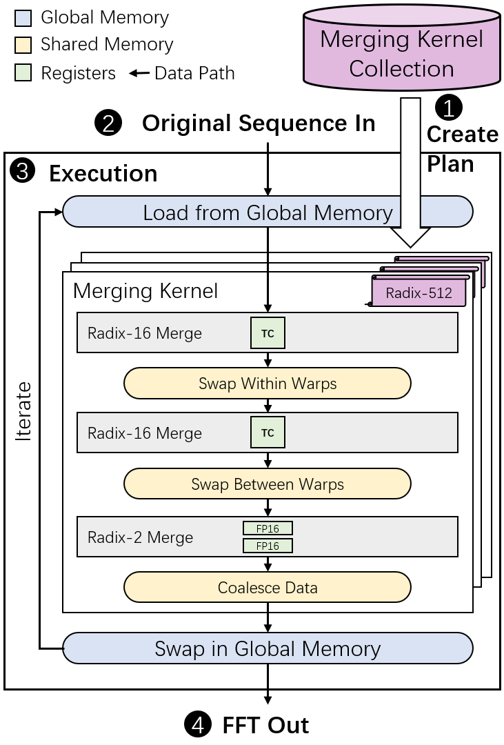
Modeled after FFTW and cuFFT, tcFFT uses a simple configuration mechanism called a plan. A plan chooses a series of optimal radix-X merging kernels. Then, when the execution function is called, actual transform takes place following the plan. Figure 1 shows the complete process of performing an FFT. First, a function is called to create a plan based on the dimension and the size of the input data. This plan selects an optimal set of merging kernels from the pre-implemented merging kernel collection. Then, the execution function is called with the plan and the original data as input. In the execution function, the previously determined merging kernels are executed in turn in multiple iterations. Meantime, multiple types of memory in GPU is fully utilized to increase the reuse of data. After all iterations are executed, the FFT of the original sequence is obtained.

By decomposing the FFT process into a series of merging kernels, we improved the code reusability and also greatly reduced the workload of subsequent performance-related optimization work.

Support FFTs of all power-of-two sizes. We have developed a series of merging kernels of different radices to support FFTs of all power-of-two sizes. The radices of these kernels cover all powers of 2 from 16 to 8192 and larger size FFTs can be realized by combining these basic kernels. Tensor Cores only provide computing power for computing $16\times 16\times 16$ GEMM, which can be used in power-of-16 radices. To implement more radices, smaller radices should be introduced. We introduced radix 2 and radix 4, for their DFT matrices only have 0, 1 and -1, and have high computational efficiency. They are computed using FP16 CUDA Cores and account for a small proportion in the total calculation time.

By implementing a collection of merging kernels of a lot of sizes, we enable tcFFT to support FFTs of all power-of-two lengths.

Support batched FFT and 2D FFT. Batched FFT and 2D FFT are of vital importance in application scenarios. 2D FFT performs FFT on each dimension of 2D sequences in turn. It can be implemented by strided batched FFT. Take a 2D FFT on an $N_{1}\times N_{2}$ row-major matrix as an example, an $N_{1}$ batch of $N_{2}$-point FFT is applied on the $N_{1}$ rows and then an $N_{2}$ batch of strided $N_{1}$-point FFT is applied on the $N_{1}$ columns. The order of these two processes can be changed but strided batched FFT is essential.

We have implemented merging kernels that support batch and strided data. Batched FFT and 2D FFT can be implemented by calling them with proper parameters. tcFFT has the following plan functions for batched 1D and 2D FFTs:

• tcfftPlan1D (tcfftHandle *plan, int nx, int batch): This function is used to create a configuration to execute FFT on a batch of 1D sequences of equal length. nx gives the length and batch is the number of sequences.

• tcfftPlan2D (tcfftHandle *plan, int nx, int ny, int batch): This function is used for FFT on batched 2D sequences. nx gives the size of the first dimension and ny is the size of the second dimension. The data are stroed in row-major, which means that the second dimension continues in memory.

These functions can create plans for batched 1D FFT and 2D FFT. They pre-selected a series of optimal merging kernels of different radices for the special size.

3.2. Merging Kernels

Input: $N_{1}\times 512$ FFTs of size $N_{2}$

Output: $N_{1}$ FFTs of size $512N_{2}$

1 $F_{16\times 16}\leftarrow$ Load Radix-16 DFT Matrix;

2 $Tw_{16\times N_{2}}\leftarrow$ Prepare Twiddle Factors while read Input;

3 Consider input data as $32N_{1}$ $In_{16\times N_{2}}$ matrices;

4

5foreach $In_{16\times N_{2}matrix}$ do

6       foreach $InFrag_{16\times 16}$ in $In_{16\times N_{2}}$ do

             /* Parallel by Warps */

7             $TwFrag_{16\times 16}\leftarrow$ load a fragment from $Tw_{16\times N_{2}}$;

             $InFrag_{16\times 16}\leftarrow InFrag_{16\times 16}\odot TwFrag_{16\times 16}$ ;

              // on FP16 units

             $OutFrag_{16\times 16}\leftarrow F_{16\times 16}\cdot InFrag_{16\times 16}$ ;

              // on Tensor Cores

8             Store $OutFrag_{16\times 16}$ to intermediate data;

9            

10       end foreach

11      

12 end foreach

13

14$Tw_{16\times 16N_{2}}\leftarrow$ Prepare Twiddle Factors;

15 Consider intermediate data as $2N_{1}$ $In_{16\times 16N_{2}}$ matrices;

16

17foreach $In_{16\times 16N_{2}matrix}$ do

18       foreach $InFrag_{16\times 16}$ in $In_{16\times 16N_{2}}$ do

             /* Parallel by Warps */

19             $TwFrag_{16\times 16}\leftarrow$ load a fragment from $Tw_{16\times 16N_{2}}$;

             $InFrag_{16\times 16}\leftarrow InFrag_{16\times 16}\odot TwFrag_{16\times 16}$ ;

              // on FP16 units

             $OutFrag_{16\times 16}\leftarrow F_{16\times 16}\cdot InFrag_{16\times 16}$ ;

              // on Tensor Cores

20             Store $OutFrag_{16\times 16}$ to intermediate data;

21            

22       end foreach

23      

24 end foreach

25

26$F_{2\times 2}\leftarrow$ Load Radix-2 DFT Matrix;

27 $Tw_{2\times 256N_{2}}\leftarrow$ Prepare Twiddle Factors;

28 Consider intermediate data as $N_{1}$ $In_{2\times 256N_{2}}$ matrices;

29

30foreach $In_{2\times 256N_{2}matrix}$ do

31       foreach $InFrag_{2\times 1}$ in $In_{2\times 256N_{2}}$ do

             /* Parallel by Threads */

32             $TwFrag_{2\times 1}\leftarrow$ load a fragment from $Tw_{2\times 256N_{2}}$;

             $InFrag_{2\times 1}\leftarrow InFrag_{2\times 1}\odot TwFrag_{2\times 1}$ ;

              // on FP16 units

             $OutFrag_{2\times 1}\leftarrow F_{2\times 2}\cdot InFrag_{2\times 1}$ ;

              // on Tensor Cores

33             Store $OutFrag_{2\times 1}$ to output data;

34            

35       end foreach

36      

37 end foreach

Algorithm 1 Radix-512 merging kernel

Algorithm 1 shows the radix-512 batched merging kernel. It takes $N_{1}$ groups of data as input. There are 512 FFT sequences of size $N_{2}$ in each group, and they will be merged into one FFT sequence of size $512N_{2}$. The merging kernel contains three sub-merging processes. Line 1-11 and line 12-21 are two radix-16 sub-merging processes accelerated by Tensor Cores and line 22-32 is a radix-2 sub-merging process. Radix-16 sub-merging kernel is the base of tcFFT.

Radix-16 sub-merging kernel. Radix-16 merging kernel is the base of tcFFT, because a $16\times 16$ matrix can fill a Tensor Core fragment, bringing the highest computational efficiency. We treat the $X_{out}$ matrix and the $X_{in}$ matrix as multiple $16\times 16$ matrices, which can be calculated in parallel. A radix-16 sub-merging kernel can execute a radix-16 merging process described by the equation $X_{out}=F_{N_{1}}\cdot(T_{N_{1}N_{2}}\odot X_{in})$ from section 2.1. Radix-16 merging process combines FFTs of 16 sequences into an FFT of a sequence of 16 times the length. Strided data layout is also supported, and we will optimize the efficiency of memory accesses in section 4.2.

As shown in line 1-11 in algorithm 1, the sub-merging process firstly loads the radix-16 DFT matrix and calculates twiddle factors while reading input. These matrices are divided into $16\times 16$ fragments and distributed to the GPU warps for parallelization. Then wraps execute matrix-multiplication with Tensor Cores and element-wise multiplication with FP16 CUDA Cores on these fragments. After that, all fragments are put together, and $N_{1}\times 512$ FFT sequences of size $N_{2}$ are merged into $N_{1}\times 32$ FFT sequences of size $16N_{2}$. Throughout the sub-merging process, intermediate results are stored in the Tensor Core fragments, we will discuss how to manipulate them efficiently in section 4.1.

Combine multiple mergings. The $\log{N}$ merging processes of the FFT algorithm requires $\log{N}$ times of memory accesses, and the arithmetic intensity of an original merging process is not large enough. To reduce the times of global memory accesses and increase the arithmetic intensity, a complete merging kernel consists of multiple sub-merging processes and uses shared memory to exchange data in the middle.

The range of data exchange taking place in the whole FFT process has different scales. Take radix-512 merging kernel as an example, after the first radix-16 merging, each warp can exchange data internally through shared memory, for it holds all the elements needed. This can be done without synchronization. After the second radix-16 merging, data are exchanged between warps also through shared memory, but a block-range synchronization is needed. After the second radix-2 merging, data exchanges between blocks are needed, which can only be done through global memory.

We implemented merging kernels so that global memory accesses are performed only when necessary and only unavoidable synchronizations are introduced. This implementation achieves the purpose of reducing bandwidth requirements and increasing arithmetic intensity.

4. Performance Optimization

4.1. Optimizations to Tensor Cores

FFT requires complex-matrix access and element-wise multiplication operations. However, they can not be performed efficiently when the data is stored as a Tensor Core fragment due to the limitations of Tensor Core APIs.

The limitations of Tensor Core APIs. NVIDIA provides Warp Matrix Multiply Accumulate (WMMA) APIs for leveraging Tensor Cores to accelerate matrix problems of the form $D=A\cdot B+C$. There are four functions as follows (NVIDIA, 2021):

• load_matrix_sync: All warp lanes loads a matrix fragment from memory, synchronously.

• store_matrix_sync: All warp lanes stores a matrix fragment to memory, synchronously.

• fill_fragment: Fill a matrix fragment with a constant value.

• mma_sync: All warp lanes perform the warp-synchronous matrix multiply-accumulate operation $D=A\cdot B+C$ or the in-place operation, $C=A\cdot B+C$.

where a fragment is an overloaded class containing a tile of a matrix distributed across registers of all threads in the warp.

However, more operations are needed to execute FFT efficiently. (1) First, the data for FFT is usually stored in complex form. Therefore, in the stage of complex-matrix loading and storing, the input fragment of a complex matrix needs to be reformatted into an imaginary matrix fragment and a real matrix fragment. (2) Second, in the stage of computation, an element-wise multiplication operation is necessary to calculate $T_{N_{1}N_{2}}\odot X_{in}$ in equation 3.

These two operations can only be done after the fragment is stored from registers to shared memory with WMMA APIs. But it is inefficient to do so, considering that eight Tensor Core units in one SM processor are capable of performing eight $4\times 4\times 4$ matrix-multiply-and-accumulate operation in one GPU clock cycle.

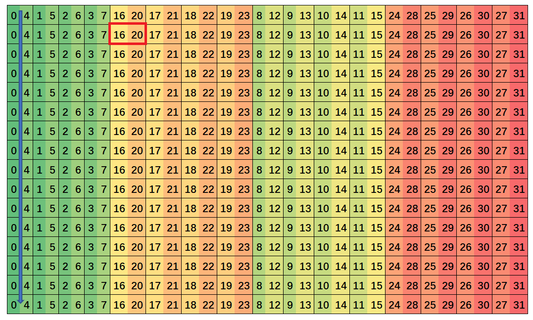
A more flexible way to work with Tensor Cores. NVIDIA does provide a method to access an individual fragment element but this can only be done uniformly, because we don’t know which elements are stored in each thread. Prior work has showed some of these element distributed maps on specific GPU models. However, these maps differ when fragment parameters change and differ on different GPU models. So we developed a tool to help obtain specific maps when needed. The map of a half datatype, $16\times 16\times 16$ shape, row-major layout, matrix_b type fragment on V100 is shown in figure 2. It is used to store tiles from the input data matrix in tcFFT. The $16\times 16$ matrix in the figure represents the matrix tile stored in this fragment. The numbers in the matrix indicate which threads in the warp store the element, for example, 16 and 20 in the second row and fifth column indicate that threads 16 and 20 have stored the element $InFrag_{2,5}$. The arrow in the first column shows the order of elements stored in thread 0, 4.

With the above maps, specified individual fragment element can be accessed. This individual element access is implemented using the fragment class member fragment::num_elements and the class member fragment::x[num_elements]. The first one keeps the num of fragment elements in this thread and the second one stores them in the above order.

Figure 2. The map of the input fragment used in tcFFT on V100: The $16\times 16$ matrix in the figure represents the matrix tile stored in this fragment. The numbers in the matrix indicate which threads in the warp store the element, for example, 16 and 20 in the second row and fifth column indicate that threads 16 and 20 have stored element $InFrag_{2,5}$. The arrow in the first column shows the order of elements stored in thread 0, 4.

Implementing FFT’s special operations efficiently. With the above method, we implemented efficient element-wise multiplications and complex matrix accesses to accelerate tcFFT. Moreover, we interleaved these two operations to hide latency.

Algorithm 2 demonstrates this process. The calc_eid function takes the fragment element map and the thread ID in a warp as parameters and returns the element id in the matrix tile. Then the thread can load the element from memory while calculating the corresponding twiddle factor and performs a complex multiplication after that. Finally, the result is assigned to the Tensor Core fragments. This process replaces the original complex matrix decomposition and element-wise multiplication operations performed in shared memory.

/* Complex-matrix access and element-wise multiplication in a thread view */

Input: fragment element map

1 fragment frag_in_real;

2 fragment frag_in_imag;

3 for $i\leftarrow 0$ to $frag\_in\_real.num\_elements-1$ do

4       eid $\leftarrow$ calc_eid (threadId, i, map);

5       half2 twiddle $\leftarrow$ get_twi(block_start, warp_start, eid);

6       half2 in_ele $\leftarrow$ In[block_start+warp_start+eid];

7       in_ele = cMul(in_ele, twiddle);

8       frag_in_real.x[i] $\leftarrow$ ele.x;

9       frag_in_imag.x[i] $\leftarrow$ ele.y;

10      

11 end for

Algorithm 2 FFT’s special operations

By developing a tool to help find the map of matrix elements into each thread’s fragment, we extended the programming methods of Tensor Cores, gained individual fragment element control, and showed how to use this method to optimize the tcFFT library. The effect of this optimization is shown and discussed in section 5.

4.2. Alleviate the Memory Bottleneck

Memory can easily become the bottleneck of FFT algorithms on GPU for two reasons: First, the original $\log{N}$ merging processes of FFT algorithm require $\log{N}$ times of global memory accesses, and the arithmetic intensity of a single merging is small. Second, merging processes in FFT require strided memory accesses, and uncoalesced strided accesses are quite inefficient on GPU. For the first problem, we have combined multiple mergings when designing tcFFT. This reduces the times of global memory accesses and increases the arithmetic intensity. For the second problem, we redesigned the data layout and memory access pattern as follows.

(a) Original out-of-place merging with a fixed data order

(b) tcFFT’s in-place merging with a changing data order; two adjacent butterflies are joined and warps can access memory with continuous size 2.

Figure 3. tcFFT’s in-place and coalesced memory access pattern: the last radix-2 merging process of an 8-point sequence as an example.

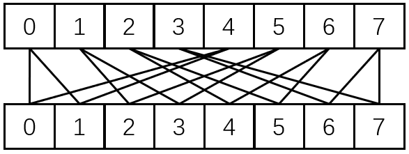
In-place computation data layout. We first used an in-place computation data layout before coalescing memory accesses. Merging is an out-of-place process when data is stored in a fixed order in multiple iterations. Figure 3(a) shows the last radix-2 merging process of an 8-point sequence as an example. The upper is the output, and the lower is the input. A pair of output elements is stored with a stride length 4. When implemented on GPU, an out-of-place algorithm requires twice the size of shared memory. This limits the continuous size that can be achieved by coalescing.

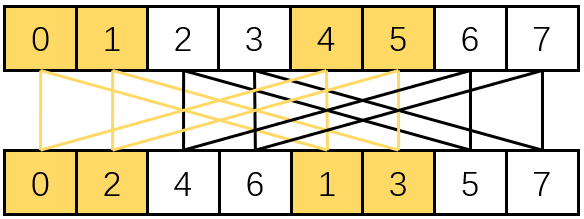
tcFFT stores data in a changing order in multiple iterations, figure 3(b) shows the same merging process in tcFFT. It rearranges the original sequence according to parity. This allows the process to be executed in place. This rearrangement is executed recursively in multiple iterations to ensure that all mergings are in-place. The actual rearrangements are based on larger changing radices, although the principle is the same.

Table 2. Achievable Global Memory Bandwidth under Different Continuous Size

Cont. Sizes	Cont. Bytes	Mem. TP. (GB/s)	BLKs
4	16	208.09	8
8	32	384.58	8
16	64	553.48	6
32	128	836.25	3
64	256	715.83	1

Coalesced global memory accesses. After in-place computation is implemented, a merging process includes multiple butterflies as shown in figure 3(b). Memory access in each butterfly is strided, but we can join adjacent butterflies together. In the figure, two adjacent butterflies are joined and warps can access memory with continuous size 2. Actually, in tcFFT, different continuous sizes are used for different radices.

Increasing the continuous size will increase continuity in memory access, but a bigger size makes a kernel use more shared memory and results in fewer concurrent blocks. To achieve higher performance, a proper continuous size is necessary. For radix-256 merging process as an example, the achievable global memory throughputs under different continuous sizes are shown in table 2. From the table, we can find that the achievable memory throughput increases as the continuous size increases when it is no more than 32. It is reasonable for the largest cache line size on GPU is 128 bytes. After that, the bandwidth drops instead. This is because that when the size exceeds 32, the number of concurrent blocks on a streaming multiprocessor reduces to one, and this will make the latency generated by block synchronization unable to be hidden.

5. Evaluation

5.1. Experimental Setup

Methods. We compare tcFFT with NVIDIA cuFFT which is the state-of-the-art FFT library on GPU. Other GPU FFT libraries are either not open source or slower than cuFFT. The version of cuFFT we used is 11.0 released in Aug. 2020. As of the time of this writing, it is the latest version on our testing DGX-2 platform and DGX-A100 platform. We compare them in terms of accuracy and performance. We show the performance of batched 1D and 2D FFTs of adequate sizes on Tesla V100 GPU and Tesla A100 GPU to evaluate the generalization of our algorithm.

Platform We measured the performance of tcFFT on two platforms, as shown in Table 3, including two generations of NVIDIA GPUs (Volta, and Ampere microarchitectures).

Table 3. Platform Information.

Platform	Volta	Ampere
GPU	Tesla V100	Tesla A100
CPU	Intel Xeon 8168	AMD Rome 7742
OS	CentOS 7	CentOS 7
CUDA	11.0	11.0
Peak FP16 (CUDA Core)	31.4 TFlops	78 TFlops
Peak FP16 (Tensor Core)	125 TFlops	312 TFlops
Memory Bandwidth	900 GB/sec	1555 GB/sec

TestCase. In the 1D performance test, we measured batched 1D FFTs of short length, moderate length and long length, from 256 to 134,217,728. For each length, we used a batch size big enough to fully utilize all the Streaming Multiprocessors and Tensor Cores. As for 2D FFT, we measured the six common lengths with adequate batch size. In the follow-up batch size test, we fixed the length, and then measured the performance versus different batch sizes. For all the tests, the input sequences were generated randomly in the interval -1.0 to 1.0.

Performance Metric. In the performance tests, the data are first transferred from CPU to GPU and a plan is created. Then, the execute function are executed thousands of times and the average performance is reported. The time spent on the data transferring and plan creating are not counted, for a plan can be reused during the whole life of real applications. We use radix-2 equivalent Trillion Floating Point Operations per Second (TFLOPS) as the Performance metric, because the total number of calculations depends on the specific radix. It can be calculated with equation 4.

(4) $$\small TFLOPS=\frac{6\times 2\times\log_{2}{N}\times N\times N\_Batch\times RepeatingTimes}{TotalTime\times 10^{12}}$$

where N denotes the length of a sequence and N_Batch denotes the num of sequences.

Precision Metric. tcFFT uses different FFT radices in the divide-and-conquer progress from common FFT algorithms, which influences the result to some degree, so we compare the relative error which is defined as equation 5.

(5) $$\small RelativeError(X)=\frac{1}{N}\sum_{i=0}^{N}\left|\frac{X_{double}[i]-X[i]}{x_{double}}\right|$$

where $X_{double}$ denotes the sequence calculated by the FFTW library in double precision. It is used as the standard result.

5.2. Precision

Table 4 shows the average relative error comparison between our tcFFT and cuFFT in 1D and 2D cases.

Table 4. Average relative error of 1D and 2D FFT, comparison between cuFFT and tcFFT

	cuFFT-1D	tcFFT-1D	cuFFT-2D	tcFFT-2D
Relative Error	1.78$\pm$0.5%	1.76$\pm$0.5%	1.65$\pm$0.1%	1.65$\pm$0.1%

tcFFT uses different merging radices from cuFFT, and the calculation processes of the two libraries differ. However, from the table, we can find that comparing with the standard result calculated by double precision FFTW, the error of the two libraries is at the same level. Although in theory, tcFFT uses matrix multiplication as the basic operator, which has better error control. But the complete progress of FFT consists of multiple mergings. It is equivalent to performing multiple matrix multiplications in turn and storing intermediate results in half precision. The storage of intermediate results is the main source of error. This process is similar in our tcFFT and cuFFT.

5.3. Overall Speedup

(a) on V100

(b) on A100

Figure 4. Performance of 1D FFT of different sizes on two platforms.

(a) on V100

(b) on A100

Figure 5. Performance of 2D FFT of different sizes on two platforms.

(a) 1D FFT

(b) 2D FFT

Figure 6. Global memory bandwidth of 1D and 2D FFT of different sizes on V100.

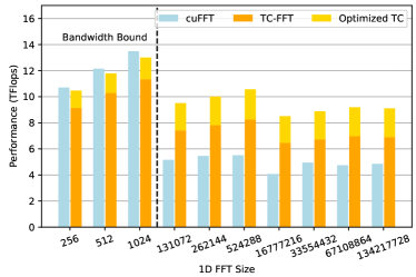
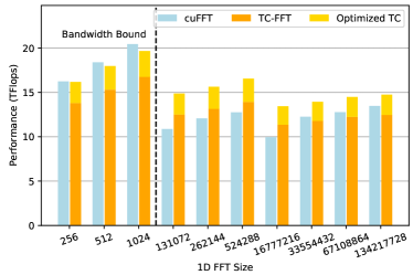
1D FFT. Figure 4(a) shows the performance comparison between our tcFFT and cuFFT on V100. As shown in the figure, the result can be roughly divided into two parts, bandwidth-bound cases and other cases. In the bandwidth-bound cases, a single sequence is short enough to be completely put into the shared memory and the core merging kernels is simple with no need of block-range thread synchronizations. Calculations can be totally overlap with memory accesses and the performance is mainly limited by the global memory bandwidth. In these cases, the memory throughput of cuFFT is close to the theoretical bandwidth peak, and our tcFFT can reach 96.4% to 97.8% performance of cuFFT. When the FFT size grows, the core merging kernels begin to use thread synchronizations which makes some calculations no longer overlap with memory accesses. In these cases, the time spent on the calculation begins to affect the overall performance and our tcFFT can achieve a minimum 1.84x speedup and an average 1.90x speedup compared with cuFFT. Figure 4(b) shows the results on A100. The results has the similar pattern to those on V100. In the bandwidth-bound cases, our tcFFT can achieve 96.1% to 99.7% performance of cuFFT. In other cases, it can achieve an average of 1.24x speedup. The benefits on A100 are less than those on V100. One reason is that, compared to V100, A100 has 2.5x half-precision computing power but only a 1.7x global memory bandwidth. As a result, optimized FFT algorithm that resorts to more computing power can only bring less performance gain.

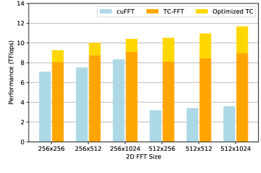
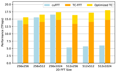
2D FFT. Figure 5(a) shows the performance of doing FFT of batched 2D sequences on V100. 2D FFT performs 1D FFTs in turn on each dimension of the data. Like cuFFT and FFTW, tcFFT use row-major order to store 2D sequences. This means that the data in the first dimension does not continue in memory and the FFT along this dimension is the main performance factor. When the size of the first dimension is 256, tcFFT is faster than cuFFT by 1.29x on average. And when the first dimension is 512 tcFFT is faster by 3.24x on average. Like long length 1D FFT, mergings along the first dimension require thread synchronizations, so this benefit comes from both improvement in calculation speed and our data arrangement design. Figure 5(b) shows the results on A100, similar to the situation of 1D FFT, performance improvement brought by tcFFT on A100 is also less than than on V100. However, tcFFT is still faster than cuFFT by 3.03x when the first dimension is 512.

The above results show that, in bandwidth-bound cases, tcFFT can use up almost all the bandwidth. And in non-bandwidth-bound cases, tcFFT can outperform cuFFT by a notable margin across different GPU architectures. This significant benefit comes from the extremely high computation power of Tensor Cores and our novel kernel optimizations.

5.4. Analysis

Since similar patterns are shown on V100 and A100, we will focus on the results on V100 in the following analysis.

(a) 1D FFT: 131072

(b) 2D FFT: $512\times 256$

Figure 7. Performance of 1D and 2D FFT of different batch sizes on V100.

Benefit of optimizations to Tensor Cores. We extended the programming methods of Tensor Cores with the fragment storage map, gained element-level control over Tensor Core fragments, and used this method to optimize tcFFT. With element-level control, tcFFT can accomplish element-wise multiplication and complex-matrix accesses without use of shared memory. This greatly reduces the latency of these operations. We shows the performance benefits of this optimization in both figure 4 and figure 5 with Optimized TC label. From the figures, we can find this optimization brings 1.15x-1.32x speedup.

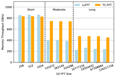
Benefit of data arrangement redesign. Figure 6(a) shows the global memory throughput of different size 1D FFTs. In the figure, we divide the sizes of 1D FFTs into three parts: short, moderate, and long, according to the required stride lengths of memory accesses. FFTs of larger sizes require longer stride lengths and use merging kernels with less computation overlap, so their memory throughput is lower. In short cases, thanks to our redesign of data arrangement and the memory access pattern, the memory throughput of tcFFT is close to the peak global memory bandwidth, and in other cases, tcFFT can outperform cuFFT nearly 2x.

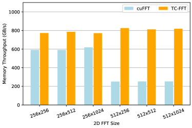
Things are similar in 2D FFT cases. Figure 6(b) shows the global memory throughput of different size 2D FFTs. The elements in the first dimension of 2D FFTs are scattered in the memory. From the figure, we can find that tcFFT obviously exceeds cuFFT in all the cases and when the size of the first dimension increases the performance of cuFFT drops a lot while that of tcFFT almost remains the same.

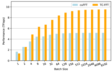
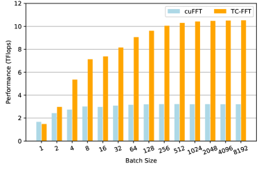
Performance of small batch sizes. The performance results above are measured with a batch size big enough to fully utilize the GPU resources. Here we give the performance results of smaller batch sizes. Figure 7(a) shows the performance comparison between our tcFFT and cuFFT when transforming batched 1D 131072-point sequences. tcFFT is faster than cuFFT when batch size is larger than 4, and the speedup ratio gradually increases. Figure 7(b) shows the performance of batched 2D $512\times 256$ FFTs. tcFFT begins to outperform cuFFT when batch size is 2. This result shows that tcFFT also performs well on small batch sizes.

6. Related Work

Accelerating HPC workload through AI-specific hardware, such as Tensor Cores, has attracted many research efforts. This work is broadly related to the researches under three topics:

Utilizing Tensor Cores for dense linear algebra. Some work utilized Tensor Cores to accelerate dense linear algebra in the performance critical steps (Abdelfattah et al., 2020; Haidar et al., 2017; Yan et al., 2020; Mukunoki et al., 2020). Haidar (Haidar et al., 2018) utilized Tensor Cores to accelerate LU factorization which solves a system of equations. EGEMM-TC (Feng et al., 2021) used precision recovery GEMM on Tensor Cores to accelerate some scientific applications. Most of the existing work focused on GEMM, convolution, or other dense linear algebra which meet the primitive of Tensor Cores. In contrast, tcFFT exploits Tensor Cores in FFT which is more challenging to be re-expressed with matrix-matrix operators.

Exploiting Tensor Cores in FFT. Sorna (Sorna et al., 2018) and Cheng (Cheng et al., 2018) gived the theoretical basis of using Tensor Cores in FFT and their example implementation resorted to cuBlas to utilized Tensor Cores. But the performance of their implementation was far inferior to cuFFT. Durran (Durrani et al., 2021) has proposed an optimized 1D FFT algorithm in their poster. Their implementation with Tensor Core WMMA APIs outperformed cuFFT and used shared memory to improved the arithmetic intensity, but only on the basic small size 1D FFT. They did not deal with the memory bottleneck caused by the unique memory access pattern of large size or multidimensional FFT, and there is still considerable room for improvement in their method to support FFT’s special operations. Different from prior work, our experimental results show that tcFFT can achieve higher performance than cuFFT in 1D and 2D FFT of universal sizes.

Implementing ditributed FFT on Heterogeneous System. Several approaches have been proposed for large size ditributed FFT on heterogeneous systems. Some work, like PFFT (Pippig, 2013) and P3DFFT (Pekurovsky, 2012), focused on how to implement distributed FFT in the highly efficient and scalable way. heFFTe (Ayala et al., 2020; Ayala et al., 2019) built a multi-node communication model for distributed FFT and achieved more than 2× speedup for the whole FFT computation. Their work focuses on the optimization of communication between computing nodes, and tcFFT can be integrated to accelerate the FFT on each node.

7. Conclusion

We design and implement tcFFT which utilizes Tensor Cores to accelerate half-precision FFT in both 1D and 2D forms of various sizes. And we exploit a set of optimizations to efficiently support FFT’s special operations and to alleviate memory bottleneck. We evaluate tcFFT and the NVIDIA cuFFT in various sizes and dimensions on the latest two generations of NVIDIA GPUs, V100 and A100. The results show that our tcFFT can outperform cuFFT 1.29x-3.24x and 1.10x-3.03x on the two GPUs, respectively. tcFFT shows a great potential to use this AI-specific hardware to accelerate FFT and the methods of tcFFT can be generalized to higher precision on higher precision Matrix Operation Units.

We have identified three major avenues for future work. First, the current version of tcFFT achieves a significant performance improvement, while it only supports half-precision. Follow-up efforts can be made to support higher precision on higher precision Matrix Operation Units; Second, tcFFT has no consideration of precision recovery. We will try to introduce some precision recovery algorithms to improve the precision of tcFFT on low precision Matrix Operation Units; Finally, as tcFFT can provide a significant speedup, we will use tcFFT in some real-world scientific applications to further confirm that tcFFT can extend the usage of Tensor Core in scientific computing.

References

- (1)
- Abdelfattah et al. (2020) Ahmad Abdelfattah, Hartwig Anzt, Erik G Boman, Erin Carson, Terry Cojean, Jack Dongarra, Mark Gates, Thomas Grützmacher, Nicholas J Higham, Sherry Li, et al. 2020. A survey of numerical methods utilizing mixed precision arithmetic. arXiv preprint arXiv:2007.06674 (2020).
- Ayala et al. (2020) Alan Ayala, Stanimire Tomov, Azzam Haidar, and Jack Dongarra. 2020. heffte: Highly efficient fft for exascale. In International Conference on Computational Science. Springer, 262–275.
- Ayala et al. (2019) Alan Ayala, Stanimire Tomov, Xi Luo, Hejer Shaeik, Azzam Haidar, George Bosilca, and Jack Dongarra. 2019. Impacts of Multi-GPU MPI collective communications on large FFT computation. In 2019 IEEE/ACM Workshop on Exascale MPI (ExaMPI). IEEE, 12–18.
- Biwer et al. (2019) Christopher Michael Biwer, Collin D Capano, Soumi De, Miriam Cabero, Duncan A Brown, Alexander H Nitz, and Vivien Raymond. 2019. PyCBC Inference: A Python-based parameter estimation toolkit for compact binary coalescence signals. Publications of the Astronomical Society of the Pacific 131, 996 (2019), 024503.
- Chen et al. (2010) Yifeng Chen, Xiang Cui, and Hong Mei. 2010. Large-scale FFT on GPU clusters. In Proceedings of the 24th ACM International Conference on Supercomputing. 315–324.
- Cheng et al. (2020) Shenggan Cheng, Hao-Ran Yu, Derek Inman, Qiucheng Liao, Qiaoya Wu, and James Lin. 2020. CUBE–Towards an Optimal Scaling of Cosmological N-body Simulations. In 2020 20th IEEE/ACM International Symposium on Cluster, Cloud and Internet Computing (CCGRID). IEEE, 685–690.
- Cheng et al. (2018) Xiaohe Cheng, Anumeena Sorna, Eduardo D’Azevedo, Kwai Wong, and Stanimire Tomov. 2018. Accelerating 2D FFT: Exploit GPU Tensor Cores through Mixed-Precision. In The International Conference for High Performance Computing, Networking, Storage, and Analysis (SC’18), ACM Student Research Poster, Dallas, TX.
- Després and Jia (2017) Philippe Després and Xun Jia. 2017. A review of GPU-based medical image reconstruction. Physica Medica 42 (2017), 76–92.
- Durrani et al. (2021) Sultan Durrani, Muhammad Saad Chughtai, Abdul Dakkak, Wen-mei Hwu, and Lawrence Rauchwerger. 2021. FFT blitz: the tensor cores strike back. In Proceedings of the 26th ACM SIGPLAN Symposium on Principles and Practice of Parallel Programming. 488–489.
- Feng et al. (2021) Boyuan Feng, Yuke Wang, Guoyang Chen, Weifeng Zhang, Yuan Xie, and Yufei Ding. 2021. EGEMM-TC: accelerating scientific computing on tensor cores with extended precision. In Proceedings of the 26th ACM SIGPLAN Symposium on Principles and Practice of Parallel Programming. 278–291.
- Frigo and Johnson (1998) Matteo Frigo and Steven G Johnson. 1998. FFTW: An adaptive software architecture for the FFT. In Proceedings of the 1998 IEEE International Conference on Acoustics, Speech and Signal Processing, ICASSP’98 (Cat. No. 98CH36181), Vol. 3. IEEE, 1381–1384.
- Gholami et al. (2015) Amir Gholami, Judith Hill, Dhairya Malhotra, and George Biros. 2015. AccFFT: A library for distributed-memory FFT on CPU and GPU architectures. arXiv preprint arXiv:1506.07933 (2015).
- Haidar et al. (2018) Azzam Haidar, Stanimire Tomov, Jack Dongarra, and Nicholas J Higham. 2018. Harnessing GPU tensor cores for fast FP16 arithmetic to speed up mixed-precision iterative refinement solvers. In SC18: International Conference for High Performance Computing, Networking, Storage and Analysis. IEEE, 603–613.
- Haidar et al. (2017) Azzam Haidar, Panruo Wu, Stanimire Tomov, and Jack Dongarra. 2017. Investigating half precision arithmetic to accelerate dense linear system solvers. In Proceedings of the 8th Workshop on Latest Advances in Scalable Algorithms for Large-Scale Systems. 1–8.
- Haynes and Côté (2000) Peter D Haynes and Michel Côté. 2000. Parallel fast Fourier transforms for electronic structure calculations. Computer physics communications 130, 1-2 (2000), 130–136.
- Jia et al. (2019) Zhe Jia, Marco Maggioni, Jeffrey Smith, and Daniele Paolo Scarpazza. 2019. Dissecting the NVidia Turing T4 GPU via microbenchmarking. arXiv preprint arXiv:1903.07486 (2019).
- Jia et al. (2018) Zhe Jia, Marco Maggioni, Benjamin Staiger, and Daniele P Scarpazza. 2018. Dissecting the NVIDIA volta GPU architecture via microbenchmarking. arXiv preprint arXiv:1804.06826 (2018).
- Liu et al. (2014) Yi-Qun Liu, Yan Li, Yun-Quan Zhang, and Xian-Yi Zhang. 2014. Memory Efficient Two-Pass 3D FFT Algorithm for Intel® Xeon Phi TM Coprocessor. Journal of Computer Science and Technology 29, 6 (2014), 989–1002.
- Maaß et al. (2011) Clemens Maaß, Matthias Baer, and Marc Kachelrieß. 2011. CT image reconstruction with half precision floating-point values. Medical physics 38, S1 (2011), S95–S105.
- Markidis et al. (2018) Stefano Markidis, Steven Wei Der Chien, Erwin Laure, Ivy Bo Peng, and Jeffrey S Vetter. 2018. Nvidia tensor core programmability, performance & precision. In 2018 IEEE International Parallel and Distributed Processing Symposium Workshops (IPDPSW). IEEE, 522–531.
- Mukunoki et al. (2020) Daichi Mukunoki, Katsuhisa Ozaki, Takeshi Ogita, and Toshiyuki Imamura. 2020. DGEMM using tensor cores, and its accurate and reproducible versions. In International Conference on High Performance Computing. Springer, 230–248.
- Nukada et al. (2012) Akira Nukada, Kento Sato, and Satoshi Matsuoka. 2012. Scalable multi-gpu 3-d fft for tsubame 2.0 supercomputer. In SC’12: Proceedings of the International Conference on High Performance Computing, Networking, Storage and Analysis. IEEE, 1–10.
- NVIDIA (2017) NVIDIA. 2017. Programming Tensor Cores in CUDA 9. Website. https://devblogs.nvidia.com/programming-tensor-cores-cuda-9/.
- NVIDIA (2021) NVIDIA. 2021. CUDA C++ Programming Guide. Website. https://docs.nvidia.com/cuda/cuda-c-programming-guide/index.html.
- Park et al. (2013) Jongsoo Park, Ganesh Bikshandi, Karthikeyan Vaidyanathan, Ping Tak Peter Tang, Pradeep Dubey, and Daehyun Kim. 2013. Tera-scale 1D FFT with low-communication algorithm and Intel® Xeon Phi™ coprocessors. In Proceedings of the International Conference on High Performance Computing, Networking, Storage and Analysis. 1–12.
- Pekurovsky (2012) Dmitry Pekurovsky. 2012. P3DFFT: A framework for parallel computations of Fourier transforms in three dimensions. SIAM Journal on Scientific Computing 34, 4 (2012), C192–C209.
- Pippig (2013) Michael Pippig. 2013. PFFT: An extension of FFTW to massively parallel architectures. SIAM Journal on Scientific Computing 35, 3 (2013), C213–C236.
- Schwaller et al. (2017) Benjamin Schwaller, Barath Ramesh, and Alan D George. 2017. Investigating TI KeyStone II and quad-core ARM Cortex-A53 architectures for on-board space processing. In 2017 IEEE High Performance Extreme Computing Conference (HPEC). IEEE, 1–7.
- Sorna et al. (2018) Anumeena Sorna, Xiaohe Cheng, Eduardo D’azevedo, Kwai Won, and Stanimire Tomov. 2018. Optimizing the fast fourier transform using mixed precision on tensor core hardware. In 2018 IEEE 25th International Conference on High Performance Computing Workshops (HiPCW). IEEE, 3–7.
- Watson and Spedding (1982) W Watson and Trevor A Spedding. 1982. The time series modelling of non-Gaussian engineering processes. Wear 83, 2 (1982), 215–231.
- Yan et al. (2020) Da Yan, Wei Wang, and Xiaowen Chu. 2020. Demystifying tensor cores to optimize half-precision matrix multiply. In 2020 IEEE International Parallel and Distributed Processing Symposium (IPDPS). IEEE, 634–643.
- Yu et al. (2018) Hao-Ran Yu, Ue-Li Pen, and Xin Wang. 2018. CUBE: an information-optimized parallel cosmological N-body algorithm. The Astrophysical Journal Supplement Series 237, 2 (2018), 24.