Hierarchical adaptive low-rank format with applications to discretized PDEs

Abstract

A novel compressed matrix format is proposed that combines an adaptive hierarchical partitioning of the matrix with low-rank approximation. One typical application is the approximation of discretized functions on rectangular domains; the flexibility of the format makes it possible to deal with functions that feature singularities in small, localized regions. To deal with time evolution and relocation of singularities, the partitioning can be dynamically adjusted based on features of the underlying data. Our format can be leveraged to efficiently solve linear systems with Kronecker product structure, as they arise from discretized partial differential equations (PDEs). For this purpose, these linear systems are rephrased as linear matrix equations and a recursive solver is derived from low-rank updates of such equations. We demonstrate the effectiveness of our framework for stationary and time-dependent, linear and nonlinear PDEs, including the Burgers’ and Allen-Cahn equations.

1 Introduction

Low-rank based data compression can sometimes lead to a dramatic acceleration of numerical simulations. A striking example is the solution of two-dimensional elliptic PDEs on rectangular domains with smooth source terms. In this case, the (structured) discretization of the source term and the solution lead to matrices that allow for excellent low-rank approximations. Under suitable assumptions on the differential operator, one can recast the corresponding discretized PDE as a matrix equation [20, 24]. In turn, this yields the possibility to facilitate efficient algorithms for matrix equations with low-rank right-hand side [7, 4]. However, in many situations of interest the smoothness property is not present in the whole domain. A typical instance are solutions that feature singularities along curves, while being highly regular elsewhere. This renders a global low-rank approximation ineffective. Adaptive discretization schemes, such as the adaptive finite element method, are one way to handle such situations. In this work, we will focus on a purely algebraic approach.

During the last decades, there has been significant effort in developing hierarchical low-rank formats that apply low-rank approximation only locally. These formats recursively partition the matrix into blocks that are either represented as a low-rank matrix or are sufficiently small to be stored as a dense matrix. These techniques are usually applied in the context of operators with a discretization known to feature low-rank off-diagonal blocks, such as integral operators with singular kernel [5]. The use of these formats for representing the solution itself has also been proposed [9, 18] but its applicability is limited by the fact that the location of the singularities needs to be known beforehand in order to define a suitable admissibility criterion [10, 11, 5]. This makes the format too inflexible to treat time-dependent problems for which the region of non-smoothness evolves over time. In the context of tensors, it has been recently proposed a bottom-up approach to identify a partitioning of the domain and perform a piecewise compression of a target tensor by means of local high-order singular value decompositions [8]. A very different and promising approach proceeds by forming high-dimensional tensors from a quantization of the function and applying the so called QTT compression format; see [14] and the references therein.

In this paper, we propose a new format that automatically adapts the choice of the hierarchical partitioning and the location of the low-rank blocks without requiring the use of an admissibility criterion. The admissibility is decided on the fly by the success or failure of low-rank approximation techniques. We call this format Hierarchical Adaptive Low-Rank (HALR) matrices.

This work focuses on the application of HALR matrices to the following class of time-dependent PDEs:

$$\begin{cases}\frac{\partial u}{\partial t}=Lu+f(t,u,\nabla u)&(x,y)\in\Omega,\quad t\in[0,T_{\max}]\\ u(x,y,0)=u_{0}(x,y)\quad\end{cases}$$ (1)

where $\Omega\subset\mathbb{R}^{2}$ is a rectangular domain, $L$ is a linear differential operator, $f$ is nonlinear and (1) is coupled with appropriate boundary conditions in space. Discretizing (1) in time with the IMEX Euler method [1] and in space with, e.g., finite differences leads to

$$(I-\Delta tL_{n})\mathbf{u}_{n,\ell+1}=\mathbf{u}_{n,\ell}+\Delta t(\mathbf{f}_{n,\ell}+\mathbf{b}_{n,\ell}),$$ (2)

where $L_{n}$ represents the discretization of the operator $L$, $\mathbf{u}_{n,\ell}$ and $\mathbf{f}_{n,\ell}$ are the discrete counterparts of $u$ and $f$ at time $t_{\ell}:=\ell\Delta t$, $\ell\in\mathbb{N}$, and $\mathbf{b}_{n,\ell}$ accounts for the boundary conditions. When using finite differences on a tensor grid, it is natural to reshape the vectors $\mathbf{u}_{n,\ell},\mathbf{f}_{n,\ell},\mathbf{b}_{n,\ell}$ into matrices $U_{n,\ell}$, $F_{n,\ell}$, $B_{n,\ell}$. In our examples, the matrix $L_{n}$ will often take the form $L_{n}=I\otimes A_{1,n}+A_{2,n}\otimes I$, a structure that is sometimes referred as having splitting-rank $2$ [24] and which allows to rephrase the linear system (2) as a linear matrix equation.

As a more specific guiding example, let us consider the two-dimensional Burgers’ equation over the unit square:

$$\frac{\partial u}{\partial t}=K\left(\frac{\partial^{2}u}{\partial x^{2}}+\frac{\partial^{2}u}{\partial y^{2}}\right)-u\cdot\left(\frac{\partial u}{\partial x}+\frac{\partial u}{\partial y}\right)\qquad(x,y)\in\Omega:=(0,1)^{2},$$ (3)

with $K>0$. Under suitably chosen boundary conditions, the solution of (3) is given by $u(x,y,t)=\left[1+\exp\left(\frac{x+y-t}{2K}\right)\right]^{-1}$; see [17, Example 3]. For a fixed time $t$, the snapshot $u_{t}:=u(\cdot,\cdot,t)$ describes a transition between two levels across the line $x+y=t$. For a small coefficient $K$ the transition becomes quite sharp, see Figure 1.

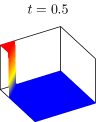
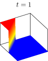
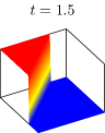
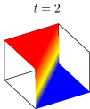
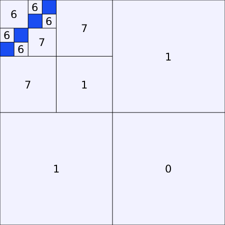
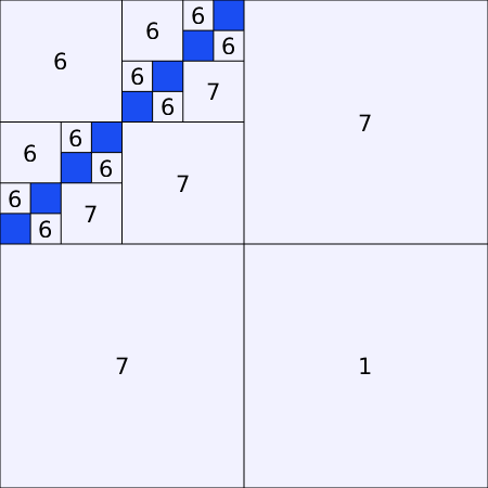
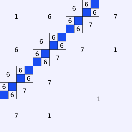
Figure 1: Top: Snapshots of $u(x,y,t)=\left[1+\exp\left(\frac{x+y-t}{2K}\right)\right]^{-1}$ for $t=0.5,1,1.5,2$ and $K=0.001$. Bottom: Corresponding block low-rank structure of $U_{n,\ell}^{\mathrm{sol}}$ for $n=4096$; the numbers indicate the rank of the corresponding block while full rank blocks are colored in blue.

Let $U_{n,\ell}^{\mathrm{sol}}$ be the matrix collecting the samples of $u_{t_{\ell}}$ on an equispaced 2D lattice; $U_{n,\ell}^{\mathrm{sol}}$ has a time dependent rank structure. More specifically, the submatrices of $U_{n,\ell}^{\mathrm{sol}}$ corresponding to subdomains which are far away from $x+y=t_{\ell}$ are numerically low-rank because they contain samples of a smooth function over a rectangular domain; see the lower part of Figure 1. Therefore, an efficient representation strategy for the solution of $\eqref{eq:burgers}$ needs to adapt the block low-rank structure of $U_{n,\ell}^{\mathrm{sol}}$ according to $\ell$.

In this work, we develop techniques for:

1. Computing a HALR representation for the discretization of a function explicitly given in terms of a black-box evaluation function.

2. Solving the linear system (2) by exploiting the HALR structure in the right-hand-side and the decomposition $L_{n}=I\otimes A_{1,n}+A_{2,n}\otimes I$.

Task (i) yields structured representations for the initial condition $\mathbf{u}_{n,0}$ and the source term $\mathbf{f}_{n,\ell}$. Taken together, Tasks (i) and (ii) allow to efficiently compute the matricized solution $U_{n,\ell+1}$ of (2). The assumption on the discretized operator in (ii) is satisfied for $L=\frac{\partial^{2}}{\partial x^{2}}+\frac{\partial^{2}}{\partial y^{2}}$ and enables us to rephrase (2) as the matrix equation

$$\left(\frac{1}{2}I-\Delta tA_{1,n}\right)U_{n,\ell+1}+U_{n,\ell+1}\left(\frac{1}{2}I-\Delta tA_{2,n}^{T}\right)=\Delta tF_{n,\ell}+U_{n,\ell}+B_{n,\ell}.$$ (4)

The paper is organized as follows; in Section 2 we introduce HALR matrices and discuss their arithmetic. Section 2.4 focuses on solving matrix equations of the form (4) where the right-hand-side is represented in the HALR format. There, we propose a divide-and-conquer method whose cost scales comparably to the memory resources used for storing the right-hand-side. In Section 3 we address the problems of constructing and adapting HALR representations. In particular, Section 3.3 considers the following scenario: given a parameter $\mathsf{maxrank}$, determine the partitioning that provides the biggest reduction of the storage cost and uses low-rank blocks of rank bounded by $\mathsf{maxrank}$. In Section 4 we incorporate HALR matrices into integration schemes for PDEs and we perform numerical tests that demonstrate the computational benefits of our approach. Conclusions are drawn in Section 5.

1.1 Notation

To simplify the statements of some definitions we introduce the following compact notation for intervals of consecutive integers:

$$\llbracket i_{l},i_{r}\rrbracket:=\{i_{l},i_{l}+1,\dots,i_{r}\}\subseteq\mathbb{N},\quad\text{ for }0<i_{l}\leq i_{r}.$$

In addition, we write $\llbracket i_{l},i_{r}\rrbracket<\llbracket i_{l}^{\prime},i_{r}^{\prime}\rrbracket$ if $i_{r}<i_{l}^{\prime}$ and we use the symbol $\sqcup$ to indicate the union of disjointed sets.

2 HALR

We are concerned with matrix partitioning described by quad-trees, i.e. trees with four branches at each node. More explicitly, given a matrix $A$ we consider the block partitioning

$$A=\begin{bmatrix}A_{11}&A_{12}\\ A_{21}&A_{22}\end{bmatrix}$$ (5)

where the blocks $A_{ij}$ can be either dense blocks, low-rank matrices, or recursively partitioned. The cases of interest are those where large portions of the matrix are in low-rank form. This is in the spirit of well established hierarchical low-rank formats such as $\mathcal{H}$-matrices [11] and $\mathcal{H}^{2}$-matrices [5]. To formalize our deliberations, we first provide the definition of a quad-tree cluster.

Definition 2.1.

Let $m,n\in\mathbb{N}$. A tree $\mathcal{T}$ is called quad-tree cluster for $\llbracket 1,m\rrbracket\times\llbracket 1,n\rrbracket$ if

• the root node is $\llbracket 1,m\rrbracket\times\llbracket 1,n\rrbracket$,

• each node $I$ is a subset of $\llbracket 1,m\rrbracket\times\llbracket 1,n\rrbracket$ of the form

  $$I=I_{r}\times I_{c}:=\llbracket m_{1},m_{2}\rrbracket\times\llbracket n_{1},n_{2}\rrbracket.$$

• each non leaf node $I=I_{r}\times I_{c}$ has $4$ children $I_{11},I_{12},I_{21},I_{22}$, that are of the form $I_{ij}=I_{r_{i}}\times I_{c_{j}}$ such that $I_{r}=I_{r_{1}}\sqcup I_{r_{2}}$, $I_{c}=I_{c_{1}}\sqcup I_{c_{2}}$, and $I_{r_{1}}<I_{r_{2}}$, $I_{c_{1}}<I_{c_{2}}$.

• Each leaf node is labeled either as dense or low-rank.

The depth of $\mathcal{T}$ is the maximum distance of a node from the root.

An example of a quad-tree cluster of depth $4$ is given in Figure 2; this induces the block structure of a $16\times 16$ matrix shown in the bottom part of the figure. This block structure is formalized in the following definition.

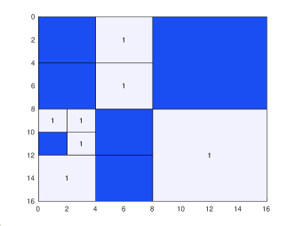
Figure 2: Example of a quad-tree cluster of depth $4$ and the induced partitioning on the matrix. The leaf nodes labeled as dense correspond to dense blocks colored in blue. The leaf nodes labeled as low-rank are taken of rank $1$ and correspond to the blocks colored in gray.

Definition 2.2.

Let $A\in\mathbb{C}^{m\times n}$ and $\mathcal{T}$ be a quad-tree cluster for $\llbracket 1,m\rrbracket\times\llbracket 1,n\rrbracket$.

1. Given $k\in\mathbb{N}$, $A$ is said to be a $(\mathcal{T},k)$ Hierarchical Adaptive Low-Rank (HALR) matrix, in short $(\mathcal{T},k)$-HALR, if for every leaf node $I_{r}\times I_{c}$ of $\mathcal{T}$ labeled as low-rank, the submatrix $A(I_{r},I_{c})$ has rank at most $k$.

2. The smallest integer $k$ for which $A$ is $(\mathcal{T},k)$-HALR is called the $\mathcal{T}$-HALR rank of $A$.

There are close connections between $(\mathcal{T},k)$-HALR matrices and $\mathcal{H}$-matrices [11]. More precisely, any $\mathcal{H}$-matrix with low-rank blocks of rank at most $k$ and with binary row and column cluster trees is a $(\mathcal{T},k)$-HALR matrix. In this case the quad-tree cluster is obtained from the Cartesian product of the row and column cluster trees. The HODLR format [10] is a special case discussed in more detail in Section 2.3. On the other hand, Definition 2.1 allows to build quad-tree clusters that can not be written as subsets of any Cartesian product of a row and a column cluster trees. For instance, we might have two nodes (not having the same father) with column indices $I_{c},I_{c^{\prime}}$ such that $I_{c}\cap I_{c^{\prime}}\neq\emptyset$ and $I_{c}\not\subseteq I_{c^{\prime}}$, $I_{c^{\prime}}\not\subseteq I_{c}$. This makes the HALR class slightly more general than $\mathcal{H}$-matrices.

In the next sections we will describe operations involving HALR matrices and we will tacitly assume to have access to their structured representations, i.e. the quad-tree clusters and the low-rank factors of the low-rank leaves. How to retrieve the HALR representation of a given matrix will be discussed in Section 3.

2.1 Matrix-vector product

In complete analogy with the $\mathcal{H}$-matrix arithmetic, the HALR structure allows to perform the matrix-vector product efficiently by relying on the block-recursive procedure described in Algorithm 1.

1:procedure HALR_MatVec($A$, $v$)

2:     if $A$ is a leaf node then

3:         return $Av$ $\triangleright$ Exploiting low-rank structure if present

4:     else

5:         Partition $v=\begin{bmatrix}v_{1}\\ v_{2}\end{bmatrix}$

6:         return $\begin{bmatrix}\textsc{HALR{}\_MatVec}(A_{11},v_{1})+\textsc{HALR{}\_MatVec}(A_{12},v_{2})\\ \textsc{HALR{}\_MatVec}(A_{21},v_{1})+\textsc{HALR{}\_MatVec}(A_{22},v_{2})\end{bmatrix}$

7:     end if

8:end procedure

Algorithm 1 Matrix-vector product with an HALR matrix $A$

In the particular case when the cluster only contains the root, $A$ itself is either low-rank (of rank $k$) or dense and Algorithm 1 requires $\mathcal{O}((m+n)k)$ and $\mathcal{O}(mn)$ flops, respectively. We remark that this cost corresponds to the memory required for storing $A$. This statement holds in more generality.

Lemma 2.3.

Let $A\in\mathbb{C}^{m\times n}$ be a $(\mathcal{T},k)$-HALR, and $v\in\mathbb{C}^{n}$ a vector. Computing $Av$ by Algorithm 1 requires $\mathcal{O}(S)$ flops, where $S$ is the memory required to store $A$.

Proof.

The result is shown by induction on the depth of $\mathcal{T}$. By the discussion above, the claim is true when $\mathcal{T}$ consists of a single node. If the result holds for trees of depth up to $d$, and $\mathcal{T}$ has depth $d+1$, the cost for $Av$ is dominated by the cost of the $4$ recursive calls to HALR_MatVec. Using the induction assumption, it follows that the cost for these calls sums up to $\mathcal{O}(S)$. ∎

2.2 Arithmetic operations

We proceed by analyzing the interplay between the quad-tree cluster partitioning and the usual matrix operations. If $A$ is a given $(\mathcal{T},k)$-HALR  we can define the transpose of $\mathcal{T}$ as the natural cluster tree for $A^{T}$.

Definition 2.4.

Let $m,n\in\mathbb{N}$ and $\mathcal{T}$ a quad-tree cluster for $\llbracket 1,m\rrbracket\times\llbracket 1,n\rrbracket$. The transposed quad-tree cluster $\mathcal{T}^{T}$ is defined as the quad-tree cluster on $\llbracket 1,n\rrbracket\times\llbracket 1,m\rrbracket$ obtained from $\mathcal{T}$ by:

1. replacing each node $I_{r}\times I_{c}$ with $I_{c}\times I_{r}$

2. swapping the subtrees at $I_{12}$ and $I_{21}$ for every non-leaf node.

Clearly, $A$ is $(\mathcal{T},k)$-HALR if and only if $A^{T}$ is $(\mathcal{T}^{T},k)$-HALR.

Remark 2.5.

In the following, we want to regard a subtree of $\mathcal{T}$ again as a quad-tree cluster. For such a subtree to satisfy Definition 2.1, we tacitly shift its root $\llbracket m_{1},m_{2}\rrbracket\times\llbracket n_{1},n_{2}\rrbracket$ to $\llbracket 1,m_{2}-m_{1}\rrbracket\times\llbracket 1,n_{2}-n_{1}\rrbracket$ and, analogously, all other nodes in the subtree. In the opposite direction, when connecting a tree to a leaf of $\mathcal{T}$, we shift the root (and the other nodes) of the tree such that it matches the index set of the leaf.

Now, let us focus on arithmetic operations between HALR matrices. When dealing with binary operations, we need to ensure some compatibility between the sizes of the hierarchical partitioning in order to unambiguously define the partitioning of the result. To this aim, we introduce the notions of row and column compatibility, which will be used in the next section for characterizing matrix products and additions.

Definition 2.6.

Given $m_{A},n_{A},m_{B},n_{B}\in\mathbb{N}$, let $\mathcal{T}_{A},\mathcal{T}_{B}$ be quad-tree clusters for $\llbracket 1,m_{A}\rrbracket\times\llbracket 1,n_{A}\rrbracket$ and $\llbracket 1,m_{B}\rrbracket\times\llbracket 1,n_{B}\rrbracket$, respectively.

• $\mathcal{T}_{A}$ and $\mathcal{T}_{B}$, with roots $I_{A}$ and $I_{B}$, are said to be row-compatible if one of the following two conditions are satisfied:

  1. $\mathcal{T}_{A}$ or $\mathcal{T}_{B}$ only contains the root, and $m_{A}=m_{B}$.

  2. For every $i,j=1,2$ the subtrees at $(I_{A})_{ij}$ and $(I_{B})_{ij}$ are row-compatible.

• $\mathcal{T}_{A}$ and $\mathcal{T}_{B}$ are said column-compatible if $\mathcal{T}_{A}^{T}$ and $\mathcal{T}_{B}^{T}$ are row-compatible.

• $\mathcal{T}_{A}$ and $\mathcal{T}_{B}$ are said compatible if they are both row- and column-compatible.

Intuitively, two quad-trees $\mathcal{T}_{A}$ and $\mathcal{T}_{B}$ are row (resp. column) compatible if taking the same path in $\mathcal{T}_{A}$ and $\mathcal{T}_{B}$ yields index sets with the same number of row (resp. column) indices.

According to Definition 2.6, compatibility does not depend on the labeling of the leaf nodes. Moreover, two clusters can be compatible even if they have different depths (or contain subtrees of different depths). The following definition introduces a partial ordering among compatible trees. This will be used to define the intersection between quad-tree clusters, which in turn allows us to characterize the natural partitioning of binary matrix operations involving $A$ and $B$.

Definition 2.7.

Let $\mathcal{T}_{A},\mathcal{T}_{B}$ be compatible quad-tree clusters for $\llbracket 1,m\rrbracket\times\llbracket 1,n\rrbracket$. We write $\mathcal{T}_{A}\leq\mathcal{T}_{B}$ if one of the following conditions is satisfied

1. $\mathcal{T}_{A}$ only contains the root labeled as low-rank.

2. $\mathcal{T}_{B}$ only contains the root labeled as dense.

3. For every $i,j=1,2$ the subtrees $(\mathcal{T}_{A})_{ij}$ and $(\mathcal{T}_{B})_{ij}$ at $(I_{A})_{ij}$ and $(I_{B})_{ij}$, respectively, verify $(\mathcal{T}_{A})_{ij}\leq(\mathcal{T}_{B})_{ij}$.

The idea behind Definition 2.7 is that $\mathcal{T}_{A}\leq T_{B}$ implies that a $(\mathcal{T}_{A},k)$-HALR matrix has a stronger structure than an $(\mathcal{T}_{B},k)$-HALR one. In fact, any $(\mathcal{T}_{A},k)$-HALR is also a $(\mathcal{T}_{B},k)$-HALR for all $\mathcal{T}_{B}\geq\mathcal{T}_{A}$. A low-rank matrix itself corresponds to the format with the strongest structure. Based on this, we define the intersection between $\mathcal{T}_{A}$ and $\mathcal{T}_{B}$ as the strongest structure among the ones which are weaker than both $\mathcal{T}_{A}$ and $\mathcal{T}_{B}$.

Definition 2.8.

Let $\mathcal{T}_{A},\mathcal{T}_{B}$ be compatible quad-tree clusters for $\llbracket 1,m\rrbracket\times\llbracket 1,n\rrbracket$. Their intersection $\mathcal{T}:=\mathcal{T}_{A}\cap\mathcal{T}_{B}$ is defined recursively as follows:

1. If $\mathcal{T}_{A}$ (resp. $\mathcal{T}_{B}$) only contain the root labeled as low-rank then $\mathcal{T}_{A}\cap\mathcal{T}_{B}=\mathcal{T}_{B}$ (resp. $\mathcal{T}_{A}\cap\mathcal{T}_{B}=\mathcal{T}_{A}$).

2. If $\mathcal{T}_{A}$ or $\mathcal{T}_{B}$ only contain the root labeled as dense then $\mathcal{T}_{A}\cap\mathcal{T}_{B}$ is a tree that only contains the root labeled as dense.

3. If $\mathcal{T}_{A}$ and $\mathcal{T}_{B}$ contain more than one node then their intersection is constructed by connecting the subtrees $\mathcal{T}_{ij}=(\mathcal{T}_{A})_{ij}\cap(\mathcal{T}_{B})_{ij}$, $i,j=1,2$, to the root $I=I_{A}=I_{B}$.

Remark 2.9.

The neutral element for the intersection is given by the quad-tree $\mathcal{T}$ only containing the root labeled as low-rank, that is, a low-rank matrix.

We now make use of the notions defined above to infer the structure of $A+B$ from the ones of $A$ and $B$.

Lemma 2.10.

Let $A,B\in\mathbb{C}^{m\times n}$ be $(\mathcal{T}_{A},k_{A})$-HALR and $(\mathcal{T}_{B},k_{B})$-HALR, respectively. If $\mathcal{T}_{A},\mathcal{T}_{B}$ are compatible then $A+B$ is $(\mathcal{T}_{A}\cap\mathcal{T}_{B},k_{A}+k_{B})$-HALR.

Proof.

We recall that the sum of two matrices of rank at most $k_{A}$ and $k_{B}$, respectively, has rank at most $k_{A}+k_{B}$. The statement follows from traversing the tree $T_{A}\cap\mathcal{T}_{B}$; for every leaf in the tree for which both submatrices of $A$ and $B$ are low rank, the resulting submatrix in $A+B$ will have rank at most $k_{A}+k_{B}$. ∎

It is instructive to consider two special cases. First, if $\mathcal{T}_{A}=\mathcal{T}_{B}$, then $A+B$ shares the same quad-tree cluster (with higher rank). Second, in view of Remark 2.9, if $A$ is low rank then $A+B$ has the same structure as $B$, with a rank increase by (at most) the rank of $A$.

The proof of Lemma 2.10 suggests a recursive procedure that is summarized in Algorithm 2. An inductive argument analogous to the one used for Lemma 2.3 shows that the complexity of Algorithm 2 is bounded by two times the cost of storing a $(\mathcal{T}_{A}\cap\mathcal{T}_{B},k_{A}+k_{B})$-HALR matrix. Note that this estimate can be reduced by exploiting the fact that Line 5 is executed at no cost by simply appending the low-rank factors of $A,B$. For example, when $A$ is a rank-$k_{A}$ matrix the cost reduces to $k_{A}$ times the number of entries in the dense blocks of $B$, which equals the storage needed for a $(\mathcal{T}_{B},0)$-HALR matrix

1:procedure HALR_Sum($A$, $B$)

2:     if $A$ and/or $B$ are leaf nodes labeled as dense then

3:         return the dense matrix $A+B$

4:     else if $A$ and $B$ are leaf nodes labeled as low-rank then

5:          return a low-rank factorization of $A+B$

6:     else

7:         If $A$ (resp. $B$) is a low-rank leaf, partition it according to $B$ (resp. $A$)

8:         return $\begin{bmatrix}\textsc{HALR{}\_Sum}(A_{11},B_{11})&\textsc{HALR{}\_Sum}(A_{12},B_{12})\\ \textsc{HALR{}\_Sum}(A_{21},B_{21})&\textsc{HALR{}\_Sum}(A_{22},B_{22})\end{bmatrix}$

9:     end if

10:end procedure

Algorithm 2 Sum of HALR matrices

For a matrix product $A\cdot B$ of HALR matrices, it is natural to assume that $A^{T}$ and $B$ are row compatible. Assuming that $\mathcal{T}_{A}$ and $\mathcal{T}_{B}$ denote, as usual, the quad-tree clusters of $A$ and $B$, the matrix product $A\cdot B$ stored in the HALR format is computed with the following procedure:

1. If $\mathcal{T}_{A}$ (resp. $\mathcal{T}_{B}$) only contains the root labeled as low-rank, then the resulting tree only contains the root labeled as low-rank and its factorization is obtained efficiently from the one of $A$ (resp. $B$); otherwise

2. if $\mathcal{T}_{A}$ (resp. $\mathcal{T}_{B}$) only contains the root labeled as dense, then $A\cdot B$ is computed in dense arithmetic and the resulting tree only contains the root labeled as dense; otherwise

3. we partition

   $$A=\begin{bmatrix}A_{11}&A_{12}\\ A_{21}&A_{22}\\ \end{bmatrix},\qquad B=\begin{bmatrix}B_{11}&B_{12}\\ B_{21}&B_{22}\\ \end{bmatrix},\qquad C=AB=\begin{bmatrix}C_{11}&C_{12}\\ C_{21}&C_{22}\\ \end{bmatrix},$$

   determine recursively $A_{ik}B_{kj}$ along with their clusters $\mathcal{T}_{ijk}$ for $i,j,k=1,2$, and set $C_{ij}=A_{i1}B_{1j}+A_{i2}B_{2j}$ with cluster $\mathcal{T}_{ij1}\cap\mathcal{T}_{ij2}$.

We note that it is difficult to predict a priori the quad-tree cluster of $AB$ because even if $A$ and $B$ contain many low-rank blocks, the structure may be completely lost in $AB$; see the example reported in Figure 3. Also computing $A\cdot B$ may cost significantly more than the storage cost of the outcome, e.g., when $A$ and $B$ are dense matrices. On the other hand, in Section 2.3 we will show that if one of the two factors happens to be a HODLR matrix then the cost of computing $A\cdot B$ and its quad-tree structure are predictable.

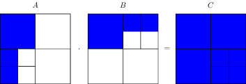
Figure 3: Example of loss of structure when computing the matrix-matrix multiplication. The blue region correspond to nodes labeled as dense, and the empty regions to nodes labeled as low-rank.

2.3 HODLR matrices

HODLR matrices are special cases of HALR matrices; all the off-diagonal blocks have low rank. To formalize this notion, we adopt the definition given in [15], rephrased in the formalism of quad-tree clusters.

Definition 2.11.

A quad-tree cluster $\mathcal{T}_{p}^{(H)}$ of depth $p$ is said to be a HODLR cluster if either $p=1$ and $\mathcal{T}_{p}^{(H)}$ only contains the root labeled as dense, or if the children $I_{ij}$ at the root of $\mathcal{T}_{p}^{(H)}$ satisfy:

• $I_{12}$ and $I_{21}$ are leaf nodes labeled as low-rank.

• the subtrees at $I_{11}$ and $I_{22}$ are HODLR clusters of depth $p-1$.

We say that a matrix is $(\mathcal{T}_{p}^{(H)},k)$-HODLR if it is $(\mathcal{T}_{p}^{(H)},k)$-HALR. The smallest integer $k$ for which a matrix $A$ is $(\mathcal{T}_{p}^{(H)},k)$-HODLR is called the HODLR rank of $A$.

An example of a HODLR cluster is reported in Figure 4. A crucial property of HODLR matrices is that they are block diagonal up to a low-rank correction. This allows to predict the structure of a product of HALR matrices whenever one of the factors is, in fact, a HODLR matrix.

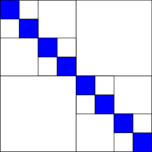
Figure 4: Example of partitioning induced by a HODLR-cluster of depth $3$.

Lemma 2.12.

Let $A\in\mathbb{C}^{m\times m}$ be a $(\mathcal{T}^{(H)}_{p_{A}},k_{A})$-HODLR matrix and $B\in\mathbb{C}^{m\times n}$ be a $(\mathcal{T},k_{B})$-HALR matrix of depth $p_{B}$. If $A^{T}$ and $B$ are row compatible and $p_{A}\geq p_{B}$, then $A\cdot B$ is a $(\mathcal{T},k_{B}+(p_{A}-1)\cdot k_{A})$-HALR matrix. Similarly, if $C$ is an $n\times n$ $(\mathcal{T}_{p_{C}}^{(H)},k_{C})$-HODLR matrix and $p_{C}\geq p_{B}$ then $B\cdot C$ is a $(\mathcal{T},k_{B}+(p_{C}-1)\cdot k_{C})$-HALR matrix

Proof.

We prove only the first statement, the second can be obtained by transposition. We proceed by induction on $p_{A}$; if $p_{A}=1$, then $A$ is composed of a single dense block. Since $p_{B}\leq p_{A}$, $B$ is also composed of a single block, either labeled as low-rank or dense. Both structures are preserved when multiplying with $A$.

Suppose that the claim is valid for $p_{A}-1\geq 1$. If $\mathcal{T}$ is composed of a single node, the claim is valid. Otherwise, by decomposing $A$ in its diagonal and off-diagonal parts, we may write

$$\begin{bmatrix}A_{11}&A_{12}\\ A_{21}&A_{22}\\ \end{bmatrix}\begin{bmatrix}B_{11}&B_{12}\\ B_{21}&B_{22}\\ \end{bmatrix}=\underbrace{\begin{bmatrix}A_{11}B_{11}&A_{11}B_{12}\\ A_{22}B_{21}&A_{22}B_{22}\\ \end{bmatrix}}_{M_{D}}+\underbrace{\begin{bmatrix}A_{12}B_{21}&A_{12}B_{22}\\ A_{21}B_{11}&A_{21}B_{12}\\ \end{bmatrix}}_{M_{O}}.$$ (6)

In view of the induction step, each block of $M_{D}$ is a $(\mathcal{T}_{ij},k_{B}+(p_{A}-2)k_{A})$-HALR matrix, for $i,j=1,2$, where $\mathcal{T}_{ij}$ are the quad-tree clusters associated with the first level of $\mathcal{T}$. In particular, $M_{D}$ is $(\mathcal{T},k_{B}+(p_{A}-2)k_{A})$-HALR. Finally, note that all the blocks of $M_{O}$ have rank bounded by $k_{A}$, and therefore $M_{O}$ is $(\mathcal{T},k_{A})$-HALR. We conclude that $AB=M_{D}+M_{O}$ is $(\mathcal{T},k_{B}+(p_{A}-1)k_{A})$-HALR. ∎

The complexity of multiplying by a HODLR matrix can be bounded in terms of the storage of the other factor.

Lemma 2.13.

Under the assumptions of Lemma 2.12 the cost of computing $A\cdot B$ is $\mathcal{O}(S(n_{\min}+k_{A}(p_{A}-1)))$ where $S$ is the storage cost of $B$ and $n_{\min}$ is an upper bound on the size of the dense diagonal blocks of $A$.

Proof.

For $p_{A}=1$, $A$ is a square matrix of size at most $n_{\min}$ while $B$ has low rank or is dense. In both cases, it directly follows that the cost of multiplication is $\mathcal{O}(Sn_{\min})$.

For the induction step, we recall the splitting (6) of $A\cdot B$ into two terms $M_{D}$ and $M_{O}$. The term $M_{O}$ is a product between $B$ and a matrix of rank (at most) $2k_{A}$, which, according to Lemma 2.3, requires $c_{v}Sk_{A}$ operations for some constant $c_{v}$. The term $M_{D}$ consists of four products $A_{ii}B_{ij}$, where $A_{ij}$ is a HODLR matrix of depth $p_{A}-1$ and $B_{ij}$ is a HALR matrix. By induction, there is a constant $c\geq c_{v}+2$ such that the cost for each of these four multiplications is bounded by $cS_{ij}(n_{\min}+k_{A}(p_{A}-2))$ operations, where $S_{ij}$ denotes the storage cost of $B_{ij}$. Adding the corresponding rank-$k_{A}$ submatrix of $M_{O}$ requires at most $2S_{ij}k_{A}$ operations, as discussed after Lemma 2.10. Therefore, the cost for computing the block $(i,j)$ of the product $A\cdot B$ is bounded by $cS_{ij}(n_{\min}+k_{A}(p_{A}-1))$. Summing over $i,j$ concludes the proof. ∎

Remark 2.14.

When performing arithmetic operations between HALR matrices, or HODLR and HALR matrices, it is often observed that the numerical rank of the blocks in the outcome is significantly less than the worst case scenario depicted in Lemma 2.10 and 2.13. Hence, it is advisable to perform a recompression stage, see [11, Algorithm 2.17, p. 33], when expanding low-rank factorizations, such as in line 5 of Algorithm 2.

2.4 Solving Sylvester equations with HODLR coefficients and HALR right-hand-side

As pointed out in the introduction, when dealing with PDEs defined on a rectangular two-dimensional domain, one frequently encounters linear matrix equations of the form

$$AX+XB=C,$$ (7)

with square matrices $A,B$ and a right-hand side $C$ of matching size. To simplify the discussion we will assume that $A$ and $B$ are of equal size $n$. As $A,B$ stem from the discretization of a 1D differential operator, they are typically $(\mathcal{T}_{p}^{(H)},k)$-HODLR for some small $k$. In contrast to our previous work [15], where we assumed $C$ to be HODLR as well, we now consider the more general setting when $C$ is $(\mathcal{T},k_{C})$-HALR. In the following, we require that $\mathcal{T}_{p}^{(H)}$ is compatible with $\mathcal{T}$ and $p\geq p_{C}$, where $p_{C}$ denotes the depth of $\mathcal{T}$.

The particular case when $C$ is a dense matrix will be discussed in further detail in Section 2.4.1. For the moment, we let DenseRHS_Sylv denote the algorithm chosen for this case. If, instead, $C$ is low-rank, well-studied low-rank solvers are available, such as Krylov subspace methods and ADI (see [23] for a survey). Under suitable conditions on the spectra of $A$ and $B$ and given a low-rank factorization of $C$, these solvers return an approximation to the solution $X$ in factorized low-rank format. Since the specific choice of the low-rank solver is not crucial for the following discussion, we refer to this routine as LowRankRHS_Sylv.

The equation (7) can be solved recursively using an extension of our divide-and-conquer approach [15] for HODLR matrices $C$. If $\mathcal{T}$ only contains the root and, hence, $C$ is composed of a single block, we use either DenseRHS_Sylv (if $C$ is dense) or LowRankRHS_Sylv (if $C$ is low-rank). Otherwise, we partition (7) according to the four children of the root of $\mathcal{T}$:

$$\begin{bmatrix}A_{11}&A_{12}\\ A_{21}&A_{22}\\ \end{bmatrix}\begin{bmatrix}X_{11}&X_{12}\\ X_{21}&X_{22}\\ \end{bmatrix}+\begin{bmatrix}X_{11}&X_{12}\\ X_{21}&X_{22}\\ \end{bmatrix}\begin{bmatrix}B_{11}&B_{12}\\ B_{21}&B_{22}\\ \end{bmatrix}=\begin{bmatrix}C_{11}&C_{12}\\ C_{21}&C_{22}\\ \end{bmatrix}.$$

In the spirit of [15], we first solve the equation associated with the diagonal blocks of $A$ and $B$:

$$\begin{bmatrix}A_{11}&0\\ 0&A_{22}\\ \end{bmatrix}\begin{bmatrix}\widetilde{X}_{11}&\widetilde{X}_{12}\\ \widetilde{X}_{21}&\widetilde{X}_{22}\\ \end{bmatrix}+\begin{bmatrix}\widetilde{X}_{11}&\widetilde{X}_{12}\\ \widetilde{X}_{21}&\widetilde{X}_{22}\\ \end{bmatrix}\begin{bmatrix}B_{11}&0\\ 0&B_{22}\\ \end{bmatrix}=\begin{bmatrix}C_{11}&C_{12}\\ C_{21}&C_{22}\\ \end{bmatrix},$$ (8)

which is equivalent to solving the four decoupled equations

$$A_{ii}\widetilde{X}_{ij}+\widetilde{X}_{ij}B_{jj}=C_{ij},\qquad i,j=1,2,\qquad\widetilde{X}:=\begin{bmatrix}\widetilde{X}_{11}&\widetilde{X}_{12}\\ \widetilde{X}_{21}&\widetilde{X}_{22}\\ \end{bmatrix},$$ (9)

where, by recursion, $\widetilde{X}$ can be represented in the $\mathcal{T}$-HALR format. Letting $\delta X:=X-\widetilde{X}$ and subtracting (8) from (7), we obtain

$$A\delta X+\delta XB=-\begin{bmatrix}0&A_{12}\\ A_{21}&0\end{bmatrix}\widetilde{X}-\widetilde{X}\begin{bmatrix}0&B_{12}\\ B_{21}&0\end{bmatrix},$$

which is a Sylvester equation with right-hand-side of rank at most $4k$. In turn, $\delta X$ is computed using LowRankRHS_Sylv, and $X=\widetilde{X}+\delta X$ is retrieved performing a low-rank update. Note that the Sylvester equations in (9) have again HODLR coefficients and HALR right-hand-side, with the depth decreased by one. Applying this step recursively yields the divide-and-conquer scheme reported in Algorithm 3. Note that, the approximate solution returned by Algorithm 3 retains the HALR format, with the quad-tree cluster $\mathcal{T}$ inherited from $C$.

1:procedure D&C_Sylv($A,B,C$)

2:     if $p_{C}=1$ then

3:         if $C$ is low-rank then

4:              return LowRankRHS_Sylv($A,B,C$)

5:         else

6:              return DenseRHS_Sylv($A,B,C$)

7:         end if

8:     else

9:         for $i,j=1,2$ do

10:              $\widetilde{X}_{ij}\leftarrow\textsc{D\&C\_Sylv}(A_{ii},B_{jj},C_{ij}$)

11:         end for

12:         $\widetilde{C}\leftarrow-\begin{bmatrix}0&A_{12}\\ A_{21}&0\end{bmatrix}\widetilde{X}-\widetilde{X}\begin{bmatrix}0&B_{12}\\ B_{21}&0\end{bmatrix}$

13:         $\delta X\leftarrow\textsc{LowRankRHS\_Sylv}(A,B,\widetilde{C})$

14:         return $\begin{bmatrix}\widetilde{X}_{11}&\widetilde{X}_{12}\\ \widetilde{X}_{21}&\widetilde{X}_{22}\\ \end{bmatrix}+\delta X$

15:     end if

16:end procedure

Algorithm 3 Divide-and-conquer approach for solving $AX+XB=C$.

In practice, LowRankRHS_Sylv in lines 4 and 13 uses low-rank factorizations of the matrices $C$ and $\widetilde{C}$, and returns the solutions in factorized form. The low-rank factors of $C$ at line 4 are given as $C$ is a leaf node of an HALR matrix. At line 4 they are easily retrieved using the low-rank factorizations of the off-diagonal blocks of $A$ and $B$ that are stored in their HODLR representations; see [15, Section 3.1] for more details. When $X$ is assembled by its blocks in line 14, an HALR structure with the appropriate tree is created.

2.4.1 Sylvester equation with dense right-hand-side

1:procedure DenseRHS_Sylv($A,B,C$)

2:     if $p_{A}=p_{B}=1$ then

3:         return DenseSolver_Sylv($A,B,C$)

4:     else

5:         Partition $C$ according to the partitioning of $A,B$:

6:         $C\leftarrow\begin{bmatrix}C_{11}&C_{12}\\ C_{21}&C_{22}\\ \end{bmatrix}\qquad$ $C_{ij}$ dense for all $i,j$

7:         for $i,j=1,2$ do

8:              $\widetilde{X}_{ij}\leftarrow\textsc{DenseRHS\_Sylv}(A_{ii},B_{jj},C_{ij}$)

9:         end for

10:         $\widetilde{C}\leftarrow-\begin{bmatrix}0&A_{12}\\ A_{21}&0\end{bmatrix}\widetilde{X}-\widetilde{X}\begin{bmatrix}0&B_{12}\\ B_{21}&0\end{bmatrix}$

11:         $\delta X\leftarrow\textsc{LowRankRHS\_Sylv}(A,B,\widetilde{C})$

12:         return $\begin{bmatrix}\widetilde{X}_{11}&\widetilde{X}_{12}\\ \widetilde{X}_{21}&\widetilde{X}_{22}\\ \end{bmatrix}+\delta X$

13:     end if

14:end procedure

Algorithm 4

We now consider the solution of a Sylvester equation (7) with dense $C$ and HODLR coefficients $A,B$. This is needed in Line 6 of Algorithm 3, but it may also be of independent interest.

For small $n$ (say, $n\leq 200$), it is most efficient to convert $A$ and $B$ to dense matrices, and use a standard dense solver, such as the Bartels-Stewart method or RECSY [13], requiring $\mathcal{O}(n^{3})$ operations.

For large $n$, we will see that it is more efficient to use a recursive approach instead of a dense solver. For this purpose, we partition $C$ into a block matrix in accordance with the row partition of $A$ and the column partition of $B$. More specifically, if the size of the minimal blocks in the partitioning of $A$ and $B$ is $n_{\min}$ and $n=2^{p}n_{\min}$, we represent $C$ as a $\frac{n}{n_{\min}}\times\frac{n}{n_{\min}}$ block matrix, that is, a $(\mathcal{T},0)$-HALR of depth $p$ with all leaf nodes labeled as dense. Then (7) is solved recursively in analogy to Algorithm 3. The resulting procedure is summarized in Algorithm 4, where DenseSolver_Sylv indicates the standard dense solver.

2.4.2 Complexity analysis of the D&C Sylvester solvers

In order to perform a complexity analysis we need to make a simplifying assumption on the convergence of the low-rank Sylvester solver, which usually depends on several features of the problem, such as the spectrum of $A$ and $B$.

Assumption 1

The computational cost of LowRankRHS_Sylv for $AX+XB=C$ is $\mathcal{O}(k_{C}kn\log n+k^{2}n\log^{2}n)$, where $n$ is the size of $A,B$, and $k$ their HODLR rank, and $k_{C}$ is the rank of $C$. The rank of $X$ is $O(k_{C})$.

Assumption 1 is satisfied, for example, if the extended Krylov subspace method [22] converges to fixed (high) accuracy in $\mathcal{O}(1)$ iterations and the LU factors of $A$ and $B$ are HODLR matrices of HODLR rank $\mathcal{O}(k)$. This requires the solution of a linear system with $A$ and $B$ in each iteration, via precomputing accurate approximations of the LU decompositions of $A$, $B$ at the beginning with cost $\mathcal{O}(k^{2}n\log^{2}n)$. In other situations, e.g., when the number of steps and/or the number of linear systems per step depend logarithmically on $n$ in order to reach a fixed accuracy, Assumption 1 and the following discussion can be easily adjusted by adding $\log n$ factors.

Before analyzing the more general Algorithm 3, it is instructive to first focus on Algorithm 4. We note that Algorithm 4 solves $(\frac{n}{n_{\min}})^{2}$ dense Sylvester equations of size $n_{\min}$ and, at each level $j=0,\ldots,p-1$, as well as $4^{j}$ Sylvester equations of size $\frac{n}{2^{j}}$ and with right-hand-sides of rank at most $4k$. In addition, computing the low-rank factorization at line 10 requires $\mathcal{O}(\frac{n^{2}}{4^{j}}k)$ operations, amounting to a total cost of $\mathcal{O}(n^{2})$. Under Assumption 1, LowRankRHS_Sylv solves the equations at level $j$ with a cost bounded by $\mathcal{O}(\frac{k^{2}n\log^{2}n}{2^{j}})$. Hence, the total computational cost is $\mathcal{O}(n^{2}(n_{\min}+k^{2}\log^{2}n))$. For large $n$ and moderate $k$, we can therefore expect that Algorithm 4 is faster than a dense solver of complexity $\mathcal{O}(n^{3})$.

The following lemma estimates the cost of Algorithm 3 for a general HALR matrix $C$, which reduces to our previous estimates in the two extreme cases: $\mathcal{O}(k_{C}kn\log n+k^{2}n\log^{2}n)$ if $C$ is low-rank and $\mathcal{O}(n^{2}n_{\min}+k^{2}n^{2}\log^{2}n)$ algorithm if $C$ is dense.

Lemma 2.15.

Consider the Sylvester equation $AX+XB=C$ with $(\mathcal{T}_{p}^{(H)},k)$-HODLR matrices $A,B\in\mathbb{C}^{n\times n}$ and a $(\mathcal{T},k_{C})$-HALR matrix $C\in\mathbb{C}^{n\times n}$, with a quad-tree cluster $\mathcal{T}$ that is compatible with $\mathcal{T}_{p}^{(H)}$ and has depth $p_{C}\leq p$. Suppose that $p\sim\log(n)$, and let $n_{\min}$ denote the size of minimal blocks in $A,B$. If Assumption 1 holds, then the cost of Algorithm 3 for computing the solution $X$ is $\mathcal{O}(S(n_{\min}+k^{2}\log^{2}n))$, where $S$ is the storage required for $C$.

Proof.

We prove the result by induction on $p_{C}$. For $p_{C}=1$, the result holds following the discussion above, because $S=n^{2}$ if $C$ is dense and $S=2k_{C}n$ if $C$ is low-rank.

As the induction step is similar to the proof of Lemma 2.13, we will keep it briefer. When $p_{C}>1$, Algorithm 3 consists of four stages:

1. Solution of $A_{ii}\widetilde{X}_{ij}+\widetilde{X}_{ij}B_{jj}=C_{ij}$, for $i,j=1,2$.
   By the induction hypothesis, each solve is $\mathcal{O}(S_{ij}(n_{\min}+k^{2}\log^{2}n))$, where $S_{ij}$ denotes the storage of $C_{ij}$ and, hence, the total cost is $\mathcal{O}(S(n_{\min}+k^{2}\log^{2}n))$.

2. Computation of the right-hand-side in line 12.
   This computation involves $4k$ matrix-vector products with $\widetilde{X}$. After $p-1$ recursive steps, the storage for $\widetilde{X}$ is at most the one for $C$ plus the one for storing the $p-1$ low-rank updates, which amounts to $\mathcal{O}(S+kpn)$ according to Assumption 1. Hence, by Lemma 2.3, the cost of this step is $\mathcal{O}(Sk+k^{2}pn)$.

3. Solution of Sylvester equation in line 13.
   Because the rank of the right-hand side is bounded by $4k$, the cost of this step step is $\mathcal{O}(k^{2}n\log^{2}n)$.

4. Update of $\widetilde{X}$ in line 14.
   The cost of this step is $\mathcal{O}(Sk+k^{2}pn)$, the storage of $\widetilde{X}$ times the rank of $\delta X$.

The total cost is dominated by the cost of Step 1, because one can easily prove by induction that $pn$ is bounded by $\mathcal{O}(S)$. This completes the proof. ∎

Note that it is not the HALR rank $k_{C}$ but the storage cost $S$ of the right-hand-side $C$ that appears explicitly in the complexity bound of Lemma 2.15. The advantage of using $S$ instead of an upper bound induced by $k_{C}$ is that it allows us to better explain why isolated relatively high ranks can still be treated efficiently.

We remark that when $A$ and $B$ are banded, e.g. when they arise from the discretization of 1D differential operators, Algorithm 3 can be executed without computing the HODLR representations of $A$ and $B$. Indeed, the low-rank factorizations of the off-diagonal blocks at line 12 are easily retrieved on the fly and one can implement a solver of Sylvester equations that exploits the sparse structure of $A,B$, in LowRankRhs_Sylv.

2.5 HALR matrices in hm-toolbox

The hm-toolbox[19] available at https://github.com/numpi/hm-toolbox is a MATLAB toolbox for working conveniently with HODLR and HSS matrices via the classes hodlr and hss, respectively. We have added functionality for HALR matrices to the toolbox. A new class halr has been introduced, which stores a $(\mathcal{T},k)$-HALR matrix $A$ as an object with the following properties:

• sz is a $1\times 2$ vector with the number of rows and columns of the matrix $A$.

• F contains a dense representation of $A$ if it corresponds to a leaf node labeled as dense.

• U, V contain the low-rank factors of $A$ if it corresponds to a leaf node labeled as low-rank.

• admissible is a Boolean flag that is set to true for leaf nodes labeled as low-rank.

• A11, A21, A12, A22 contain $4$ halr objects corresponding to the children of $A$.

The toolbox implements operations between halr objects, such as Algorithms 1–2 and matrix multiplication, as well as the Sylvester equation solver described in Section 2.4. Similar to hodlr and hss, when arithmetic operations are performed recompression (e.g., low-rank approximation) is applied in order to limit storage while ensuring a relative accuracy. More specifically, an estimate of the norm of the result $C=A\ \mathrm{op}\ B$ is computed beforehand, and recompressions are performed using a tolerance $\epsilon\cdot\lVert C\rVert$, where $\epsilon$ is a global tolerance.

3 Construction via adaptive detection of low-rank blocks

In this section we deal with task (i) described in the introduction, that is: given a function handle $f:\llbracket 1,m\rrbracket\times\llbracket 1,n\rrbracket\rightarrow\mathbb{C}$ construct an HALR representation of $A=(a_{ij})_{i,j}\in\mathbb{C}^{m\times n}$ such that $a_{ij}=f(i,j)$.

3.1 Low-rank approximation

We start by considering a simpler problem, the (global) approximation of $A$ with a low-rank matrix. Several methods have been proposed for this problem [12, 2, 25, 21], which target different scenarios. In the following sections we will often need to determine if a matrix is sufficiently low-rank in the sense that it can be approximated, within a certain accuracy, with a matrix of rank bounded by $\mathsf{maxrank}$. For this purpose, we assume the availability of a procedure $(U,V,\mathrm{flag})=\mathrm{LRA}(A,\mathsf{maxrank},\epsilon)$ that returns a low-rank factorization $A\approx UV^{T}$, of rank at most $\mathsf{maxrank}$. The returned flag indicates whether the approximation verifies $\lVert A-UV^{T}\rVert\lesssim\epsilon$.

In our implementation, we will rely on the adaptive cross approximation (ACA) algorithm with partial pivoting [2], which only requires the evaluation of a few matrix rows and columns selected by the algorithm. The parameter $\epsilon$ is used in the heuristic stopping criterion of the method, which in practice usually ensures the requirement on the absolute error stated above. When aiming at a relative accuracy $\epsilon_{\mathsf{rel}}$, we need to set $\epsilon=\epsilon_{\mathsf{rel}}\lVert A\rVert$; if $\lVert A\rVert$ is not available, it is estimated during the first ACA steps. The cost of ACA for returning an approximation of rank $k$ is $\mathcal{O}((k^{2}+kc_{A})(m+n))$ where $c_{A}$ is the cost of evaluating one entry of $A$. The approximation is returned in factorized form as a product of $m\times k$ and $k\times n$ matrices and therefore the storage cost is $\mathcal{O}(k(m+n))$.

Depending on the features of $A$, other choices for the procedure LRA might be attractive. For instance, if the matrix-vector product by $A$ and $A^{T}$ can be performed efficiently (for instance when $A$ is sparse), then a basis for the column range of $A$ can be well-approximated by taking matrix-vector products with a small number of random vectors, and this can be used to construct an approximate low-rank factorization as described in [12]. The methodology described in the following sections can be adapted to this context, by replacing the procedure LRA.

3.2 HALR approximation with prescribed cluster

Letting $\mathcal{T}$ denote a prescribed quad-tree cluster on $\llbracket 1,m\rrbracket\times\llbracket 1,n\rrbracket$, we consider the problem of approximating $A$ within a certain tolerance $\epsilon$, with a $(\mathcal{T},k)$-HALR $\widetilde{A}$ for some, hopefully small $k$. A straightforward strategy for building $\widetilde{A}$ is to perform the following operations on its blocks:

1. for a leaf node labeled low-rank, run LRA (without limitation on the rank) to approximate the block in factored form;

2. for a leaf node labeled dense, assemble and explicitly store the whole block;

3. for a non-leaf node, proceed recursively with its children.

To avoid an overestimation of the ranks for blocks of relatively small norm, we first approximate the norm of the entire matrix with the norm of a rough approximation of $A$ obtained by running LRA for a small value of $\mathsf{maxrank}$.

3.3 HALR approximation with prescribed maximum rank

We now discuss the problem at the heart of HALR: Given an integer $\mathsf{maxrank}$ determine a quad-tree cluster $\mathcal{T}$ and an $(\mathcal{T},\widetilde{k})$-HALR matrix $\widetilde{A}$ such that $\widetilde{k}\leq\mathsf{maxrank}$ and $\lVert A-\widetilde{A}\rVert\leq\epsilon$. Moreover, we ideally want $\mathcal{T}$ to be minimal in the sense that if $\hat{A}$ is another $(\hat{\mathcal{T}},\hat{k})$-HALR approximating $A$ within the tolerance $\epsilon$, and $\hat{k}\leq\mathsf{maxrank}$, then $\hat{\mathcal{T}}\not<\mathcal{T}$. In this context, we consider all the trees (or subtrees) that contain only dense leaves to be equivalent to a single dense node.

We propose to compute $\mathcal{T}$ and $\widetilde{A}$ with the following greedy algorithm:

1. We apply LRA limited by $\mathsf{maxrank}$ to the matrix $A$. If this is successful, as indicated by the returned flag, then $\mathcal{T}$ is set to a tree with a single node that is labeled low-rank and contains the approximation returned by LRA.

2. If LRA fails and the size of $A$ is smaller than a fixed parameter $n_{\min}$ then $\mathcal{T}$ is set to a tree with a single node labeled as dense and the matrix is formed explicitly.

3. Otherwise we split $A$ in $4$ blocks of nearly equal sizes and we proceed recursively on each block. Then:

   • If the $4$ blocks are all leaves labeled as dense, then we merge them into a single dense block.

   • Otherwise, we attach to the root of $\mathcal{T}$ the four subtrees resulting from the recursive calls.

The whole procedure is summarized in Algorithm 5.

1:procedure HALR_Adaptive($A,\mathsf{maxrank},\epsilon$)

2:     $(m,n)\leftarrow\textsc{size}(A)$

3:     $(U,V,\mathrm{flag})\leftarrow\textsc{LRA}(A,\mathsf{maxrank},\epsilon)$

4:     if LRA succeeds then

5:         $H.U\leftarrow U$, $H.V\leftarrow V$, $H.\mathrm{admissible}=1$

6:     else

7:         if $\min\{m,n\}\leq n_{\min}$ then

8:              $H.F\leftarrow A$, $H.\mathrm{admissible}=0$

9:         else

10:              $H.\mathrm{admissible}=0$, $m_{1}\leftarrow\lceil\frac{m}{2}\rceil,n_{1}\leftarrow\lceil\frac{n}{2}\rceil$

11:              $H.A_{11}=\textsc{HALR{}\_Adaptive}(A(1:m_{1},1:n_{1}),\mathsf{maxrank},\epsilon)$

12:              $H.A_{21}=\textsc{HALR{}\_Adaptive}(A(m_{1}+1:m,1:n_{1}),\mathsf{maxrank},\epsilon)$

13:              $H.A_{12}=\textsc{HALR{}\_Adaptive}(A(1:m_{1},n_{1}+1:n),\mathsf{maxrank},\epsilon)$

14:              $H.A_{22}=\textsc{HALR{}\_Adaptive}(A(m_{1}+1:m,n_{1}+1:n),\mathsf{maxrank},\epsilon)$

15:              if $A_{ij}$ are labeled as dense for $i,j=1,2$ then

16:                  $H.F\leftarrow\left[\begin{array}[]{cc}H.A11.F&H.A12.F\\ H.A21.F&H.A22.F\\ \end{array}\right]$

17:                  $H.A_{ij}\leftarrow[\ ]$ $\triangleright$ Remove the children

18:              end if

19:         end if

20:     end if

21:end procedure

Algorithm 5 Approximation of a matrix $A$ using the greedy construction of the quad-tree cluster $\mathcal{T}$. The (absolute) approximation accuracy is determined by $\epsilon$.

3.4 Refining an existing partitioning

As operations are performed on a $(\mathcal{T},k_{A})$-HALR matrix $A$, its low-rank properties may evolve and it can be beneficial to readjust the tree $\mathcal{T}$ accordingly by making use of Algorithm 5. More specifically, we refine $\mathcal{T}$ by performing the following steps from bottom to top:

1. Algorithm 5 with maximum rank $\mathsf{maxrank}$ is applied to each leaf node and the leaf node is replaced with the outcome.

2. A node with $4$ children that are dense leaf nodes is merged into a single dense leaf node.

3. For a node with $4$ children that are low-rank leaf nodes, we form the low-rank matrix obtained by merging them. If its numerical rank is bounded by $\mathsf{maxrank}$, we replace the node with a low-rank block. Otherwise, the node remains unchanged.

The procedure is summarized in Algorithm 6; to decide whether to merge four low-rank blocks in (iii), we make use of the method CompressFactors that computes a reduced truncated singular value decomposition of $UV^{T}$; this requires $\mathcal{O}(k^{2}(m+n)+k^{3})$ flops, where $k$ is the number of columns of $U,V$, see [11, Algorithm 2.17, p. 33].

In the next sections, Algorithm 6 is regularly used to deal with situations where a matrix $B$ is obtained from operating with $\ell$ HALR matrices $A_{1},\ldots,A_{\ell}$ and its tree is initially set to the intersection of the cluster trees of $A_{1},\ldots,A_{\ell}$. A relevant special case is the one where only $A_{1}$ is a general HALR matrix and all the other matrices are low-rank; in this case the initial tree for $B$ is the one of $A_{1}$.

1:procedure RefineCluster($A,\mathsf{maxrank},\epsilon$)

2:     if A is leaf node then

3:         $A\leftarrow\textsc{HALR{}\_Adaptive}(A,\mathsf{maxrank},\epsilon)$

4:     else

5:         $A.A_{ij}\leftarrow\textsc{RefineCluster}(A.A_{ij},\mathsf{maxrank},\epsilon)$ for $i,j=1,2$.

6:         if $A.A_{ij}$ are dense leaf nodes for $i,j=1,2$ then

7:              $A.F\leftarrow\begin{bmatrix}A.A_{11}.F&A.A_{12}.F\\ A.A_{21}.F&A.A_{22}.F\\ \end{bmatrix}$

8:         end if

9:         if $A.A_{ij}$ are low-rank leaf nodes for $i,j=1,2$ then

10:              $U\leftarrow\begin{bmatrix}A.A_{11}.U&A.A_{12}.U&&\\ &&A.A_{21}.U&A.A_{22}.U\end{bmatrix}$

11:              $V\leftarrow\begin{bmatrix}A.A_{11}.V&&A.A_{21.V}\\ &A.A_{12}.V&&A.A_{22}.V\\ \end{bmatrix}$

12:              $(U,V)\leftarrow\textsc{CompressFactors}(U,V,\epsilon)$ $\triangleright$ [11, Algorithm 2.17, p. 33]

13:              if $\mathrm{rank}(UV^{T})\leq\mathsf{maxrank}$ then

14:                  $(A.U,A.V)\leftarrow(U,V)$

15:                  $A.\mathrm{admissible}\leftarrow 1$

16:                  $A.A_{ij}\leftarrow[\ ]$ for $i,j=1,2$

17:              end if

18:         end if

19:     end if

20:end procedure

Algorithm 6

4 Numerical examples

In Sections 2 and 3 we have developed all the tools needed to implement an efficient implicit time integration scheme for the reaction diffusion equation (1), provided that the discretization of the operator $L$ has the Kronecker sum structure $I\otimes A_{n}+B_{n}\otimes I$. In the following, we describe in detail how to put all pieces together for the representative case of the Burgers’ equation. Then we provide numerical tests for other problems that can be treated similarly. The experiments have been run on a server with two Intel(R) Xeon(R) E5-2650v4 CPU with 12 cores and 24 threads each, running at 2.20 GHz, using MATLAB R2017a with the Intel(R) Math Kernel Library Version 11.3.1. In all case studies, the relative truncation threshold has been set to $\epsilon_{\mathsf{rel}}=10^{-8}$.

4.1 Burgers’ equation

We consider the following Burgers’ equation [17, Example 3] with Dirichlet boundary conditions:

$$\begin{cases}\displaystyle\frac{\partial u}{\partial t}=K\left(\frac{\partial^{2}u}{\partial x^{2}}+\frac{\partial^{2}u}{\partial y^{2}}\right)-u\cdot\left(\frac{\partial u}{\partial x}+\frac{\partial u}{\partial y}\right)=0&(x,y)\in\Omega=(0,2)\times(0,2),\\ \displaystyle u(x,y,t)=\frac{1}{1+\text{exp}((x+y-t)/2K)}&\text{for }t=0\text{ or }(x,y)\in\partial\Omega,\end{cases}$$

for $K=0.001$. We make use of a uniform finite differences discretization in space, with step $h=\frac{2}{n-1}$, combined with a Euler IMEX method for the discretization in time with step $\Delta t=5\cdot 10^{-4}$. This yields

$$\left(\frac{1}{2}I-\Delta tA_{n}\right)U_{n,\ell+1}+U_{n,\ell+1}\left(\frac{1}{2}I-\Delta tA_{n}\right)=U_{n,\ell}+\Delta t(F_{n,\ell}+B_{n,\ell}),$$ (10)

where, denoting with $\circ$ the Hadamard (component-wise) product, we have set

$$F_{n,\ell} :=U_{n,\ell}\circ\left[D_{n,\ell}U_{n,\ell}+U_{n,\ell}D_{n,\ell}^{T}+(e_{n}v_{n,\ell}^{T}+v_{n,\ell}e_{n}^{T})/h\right], (v_{n,\ell})_{j}=u(jh,2,\ell\Delta t),$$

$$B_{n,\ell} :=(e_{1}w_{n,\ell+1}^{T}+w_{n,\ell+1}e_{1}^{T}+e_{n}v_{n,\ell+1}^{T}+v_{n,\ell+1}e_{n}^{T})/h^{2}, (w_{n,\ell})_{j}=u(jh,0,\ell\Delta t)$$

and

$$A_{n}=\frac{1}{h^{2}}\begin{bmatrix}-2&1\\ 1&-2&\ddots\\ &\ddots&\ddots&1\\ &&1&-2\end{bmatrix},\qquad D_{n,\ell}=\frac{1}{h}\begin{bmatrix}-1&1\\ &\ddots&\ddots\\ &&\ddots&1\\ &&&-1\end{bmatrix}.$$

Note that $\mathrm{rank}(B_{n,\ell})\leq 4$. The time stepping procedure is reported in Algorithm 7.

1:procedure Burgers_IMEX($n$, $\Delta t$, $T_{\max}$)

2:     $h\leftarrow\frac{2}{n-1}$

3:     $\left(U_{n,0}\right)_{ij}\leftarrow u(ih,jh,0)$

4:     $t\leftarrow 0$, $\ell\leftarrow 0$

5:     while $t\leq T_{\max}$ do

6:         $F_{n,\ell}\leftarrow U_{n,\ell}\circ\left[D_{n,\ell}U_{n,\ell}+U_{n,\ell}D_{n,\ell}^{T}+(e_{n}v_{n,\ell}^{T}+v_{n,\ell}e_{n}^{T})/h\right]$

7:         $B_{n,\ell}\leftarrow(e_{1}w_{n,\ell+1}^{T}+w_{n,\ell+1}e_{1}^{T}+e_{n}v_{n,\ell+1}^{T}+v_{n,\ell+1}e_{n}^{T})/h^{2}$

8:         $R\leftarrow U_{n,\ell}+\Delta t(F_{n,\ell}+B_{n,\ell})$

9:         $U_{n,\ell+1}\leftarrow\textsc{Lyap}(\frac{1}{2}I-\Delta tA_{n},R)$$\triangleright$ Solve the Lyapunov equation (10)

10:         $t\leftarrow t+\Delta t$,   $\ell\leftarrow\ell+1$

11:     end while

12:end procedure

Algorithm 7 Time stepping procedure for the Burgers’ equation

If Algorithm 7 is executed with standard dense numerical linear algebra each time step requires $\mathcal{O}(n^{3})$ flops and $\mathcal{O}(n^{2})$ storage. In order to exploit the additional structure observed in Figure 1 we propose to maintain the HALR representations of the matrices $F_{n,\ell}$ and $U_{n,\ell}$. In particular:

1. At line 3 we employ Algorithm 5 to retrieve a quad-tree cluster tree $\mathcal{T}$ and a $(\mathcal{T},\widetilde{k})$-HALR representation of $U_{n,0}$. The rank $\widetilde{k}$ satisfies $\widetilde{k}\leq\mathsf{maxrank}$.

2. In place of lines 6–8 we compute a $(\mathcal{T},k_{R})$-HALR representation for $R$ using the algorithm described in Section 3.2. More specifically, we force the quad-tree cluster to be the one of $U_{n,\ell}$. We remark that an efficient handle function for evaluating the entries of $R$ is obtained by leveraging the HALR structure of $F_{n,\ell},U_{n,\ell}$ and the low-rank structure of $B_{n,\ell}$.

3. We refine the cluster tree of $R$ using Algorithm 6. During this process, the truncation is performed according to a relative threshold $\epsilon_{\mathsf{rel}}=10^{-5}$, comparable with the accuracy of the time integration method. This avoids taking into account the increase of the rank caused by the accumulation of the errors.

4. Since the Lyapunov equation (10) has HODLR coefficients and HALR right-hand-side we employ Algorithm 3 for its solution at line 9. Consequently, the matrix $U_{n,\ell+1}$ inherits the same quad-tree cluster of $R$.

Note that the refinement of the cluster at step (iii) is the only operation that can modify the quad-tree cluster used to represent the solution. The test has been repeated for $\mathsf{maxrank}=25,50,75,100$. In Table 1 we report the total computational time (labeled as $T_{\mathrm{tot}}$), and the maximum memory consumption for storing the solution in each run, measured in MB. We also report the total time spent solving Lyapunov equations (phase $(iv)$, labeled as $T_{\mathrm{lyap}}$) and approximating the right-hand-side and adapting the HALR structure (phases $(ii)$–$(iii)$, labeled as $T_{\mathrm{adapt}})$. These two phases accounts for most of the computational cost (between $85\%$ and $90\%$); the solution of the Lyapunov equation is the most expensive operation. The ratio $T_{\mathrm{lyap}}/T_{\mathrm{adapt}}$ seems to grow with $n$, and is around $2$ at $n=16384$.

Figure 5 describes in detail the case $\mathsf{maxrank}=50$. The solution at time $t=0$ has a low-rank structure; the region where the shock happens is confined to the origin in $[0,2]^{2}$. After some iterations, the shock moves causing an increase in the rank required to approximate the solution, and the method switches to the HALR structure. When the time approaches $t=3.75$, the solution becomes numerically low-rank again, because the shock moves close to top-right corner of $[0,2]^{2}$. This progression is reported in the top part of Figure 5, which shows the time required for each iteration, and the structure adopted by the method. We remark that since the 1D Laplacian can be diagonalized via the sine transform, Algorithm 7 can be efficiently implemented also without exploiting the local low-rank structure. In particular, the iteration cost becomes $\mathcal{O}(n^{2}\log(n))$. In the left part of Table 2 we have reported the times required by a dense version of Algorithm 7 for integrating (3) where any hierarchical structure is ignored, and the Lyapunov equations are solved by diagonalizing the Laplace operator using the FFT; for this case, we have also reported the average time for solving the Lyapunov equation via fast diagonalization; we see that leveraging the HALR structure makes the algorithm faster since dimension 8192.

The bottom plot of Figure 5 shows the absolute approximation error in the discrete $l^{2}$-norm, computed comparing the numerical solution with the true solution $u(x,y,t)=\left[1+\exp\left(\frac{x+y-t}{2K}\right)\right]^{-1}$. The error curve associated with the implementation of Algorithm 7 in dense arithmetic matches the one reported in Figure 5 confirming that the low-rank truncations have negligible effects on the computed solution. We remark that the displayed errors come from the discretization, and are not introduced by the low-rank approximations in the blocks: we have verified the computations using dense unstructured matrices, obtaining the same results.

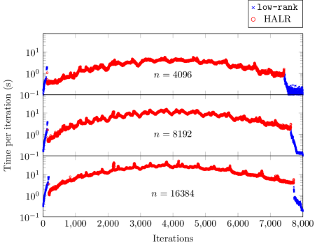
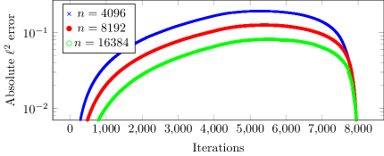
Figure 5: Top figure: time required for solving the Lyapunov equation and the adaptive approximation at each iteration; the iterations marked as low-rank correspond to the case where the matrix has the trivial partitioning with only one block labeled as low-rank; bottom figure: approximation error during the iteration, obtained computing the $l^{2}$-norm of the difference with the exact solution. The reported timings are for $\mathsf{maxrank}=50$, and $n=4096$, $n=8192$, and $n=16384$. The reported errors are absolute; for comparison, note that the $\ell^{2}$ norm of the solution grows monotonically from $0$ to $1$ in the time interval $[0,4]$, as the solution converges pointwise to $1$.

$\mathsf{maxrank}=25$ $\mathsf{maxrank}=50$ $n$ $T_{\mathrm{tot}}$ (s) $T_{\mathrm{lyap}}$ (s) $T_{\mathrm{adapt}}$ (s) Mem. $T_{\mathrm{tot}}$ (s) $T_{\mathrm{lyap}}$ (s) $T_{\mathrm{adapt}}$ (s) Mem. $4096$ $\mathbf{20057.6}$ $9742.6$ $7256.7$ $13.1$ $22334.0$ $10604.3$ $7767.4$ $\mathbf{10.3}$ $8192$ $\mathbf{54659}$ $29231.1$ $17104.5$ $17.8$ $57096.9$ $32116.9$ $17346.2$ $\mathbf{16.4}$ $16384$ $132238.3$ $80762.6$ $36539.2$ $\mathbf{25.3}$ $\mathbf{119130.4}$ $76431.5$ $31011.5$ $35.3$ $\mathsf{maxrank}=75$ $\mathsf{maxrank}=100$ $n$ $T_{\mathrm{tot}}$ (s) $T_{\mathrm{lyap}}$ (s) $T_{\mathrm{adapt}}$ (s) Mem. $T_{\mathrm{tot}}$ (s) $T_{\mathrm{lyap}}$ (s) $T_{\mathrm{adapt}}$ (s) Mem. $4096$ $26727.0$ $12915.1$ $8923.3$ $10.8$ $29383.2$ $14174.7$ $10362.5$ $12.1$ $8192$ $59340.9$ $33756.1$ $18825.8$ $22.4$ $63150.1$ $34108.4$ $22163.0$ $24.8$ $16384$ $119602.0$ $71187.1$ $35398.9$ $46.5$ $125688.6$ $71050.3$ $40701.3$ $50.4$

Table 1: Time and storage required for integrating the Burgers’ equation from $t=0$ to $t=4$, for different values of $n$ and of $\mathsf{maxrank}$. The best times and memory usage for a given $n$ are reported in bold. The reported memory is measured in Megabytes (MB), and is the maximum memory consumption for storing the solution during the iterations. The reported timings are the cumulative ones for $8000$ time steps.

FFT-based algorithms
Burgers Allen-Cahn $n$ $T_{\mathrm{tot}}$ (s) Avg. $T_{\mathrm{lyap}}$ (s) $T_{\mathrm{tot}}$ (s) Avg. $T_{\mathrm{lyap}}$ (s) $4096$ $18094$ $2.26$ $174.97$ $0.44$ $8192$ $70541$ $8.82$ $847.3$ $2.12$ $16384$ $295507$ $36.94$ $2967$ $7.42$

Table 2: Time required for integrating the Burgers’ equation and the Allen-Cahn equation, for different values of $n$, relying on sine and cosine transforms. The time step is chosen as in the experiments using the HALR structure.

4.2 Allen-Cahn equation

The Allen-Cahn equation is a reaction-diffusion equation which describes a phase separation process. It takes the following form:

$$\begin{cases}\displaystyle\frac{\partial u}{\partial t}+\nu\left(-\Delta\right)u=g(u)&\text{in }\Omega,\\[8.0pt] \displaystyle\frac{\partial u}{\partial\vec{n}}=0&\text{on }\partial\Omega,\\[8.0pt] u(x,y,0)=u_{0}(x,y),\end{cases}$$ (11)

where $\nu=5\cdot 10^{-5}$ is the mobility, $\Omega=[0,1]^{2}$ and the source term is the cubic function $g(u):=u(u-0.5)(1-u)$. This test problem is described in [6]. For a fixed choice of $(x,y)$, the solution $u(x,y,t)$ converges either to $1$ or $0$ for most points inside the domain as $t\to\infty$.

We discretize the problem with the IMEX implicit Euler method in time and centered finite differences in space, exactly as in the Burger’s equation example. The only difference is that in this problem we are considering Neumann boundary conditions instead of Dirichlet.

In this example we choose the initial (discrete) solution randomly, distributed as $u(x_{i},y_{j},0)\sim N(\frac{1}{2},1)$, with every grid point independent of the others. Integrating the system yields a model for spinodal decompositions [6]. We remark that with this choice the matrix $U_{n,0}$ has no low-rank structure, and will be treated as a dense matrix. On the other hand, during the time evolution, the smoothing effect of the Laplacian makes the solution $U_{n,\ell}$ well-approximable by low-rank matrices, at least locally (see Figure 6). For even larger $\ell$, the solution converges to either $0$ or $1$, giving rise to several “flat regions”, which can be approximated by low-rank blocks, and the structure $U_{n,\ell}$ can be efficiently memorized using a $(\mathcal{T},k)$-HALR representation.

We have integrated the solution for $t\in[0,40]$, using $\Delta t=0.1$, and grid sizes from $1024$ up to $16384$. The simulation has been run for $\mathsf{maxrank}=25,50,75,100$. The time and storage used for the integration has been reported in Table 3, analogously to the Burgers’ equation case. Note that here the maximum memory consumption is always attained at $t=0$, where the solution is stored as a dense matrix.

Figure 6 and 7 focus on the case $n=4096$ and $\mathsf{maxrank}=50$. The evolution in time of the solution and of the corresponding HALR structure are reported in Figure 6.

$t=0.3$

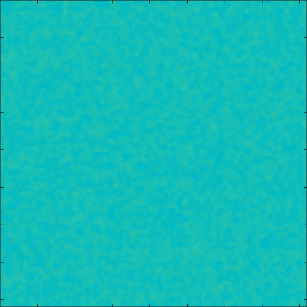
$t=0.5$

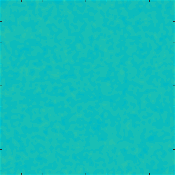
$t=18.0$

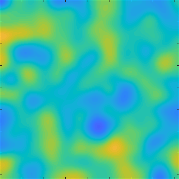
$t=35.0$

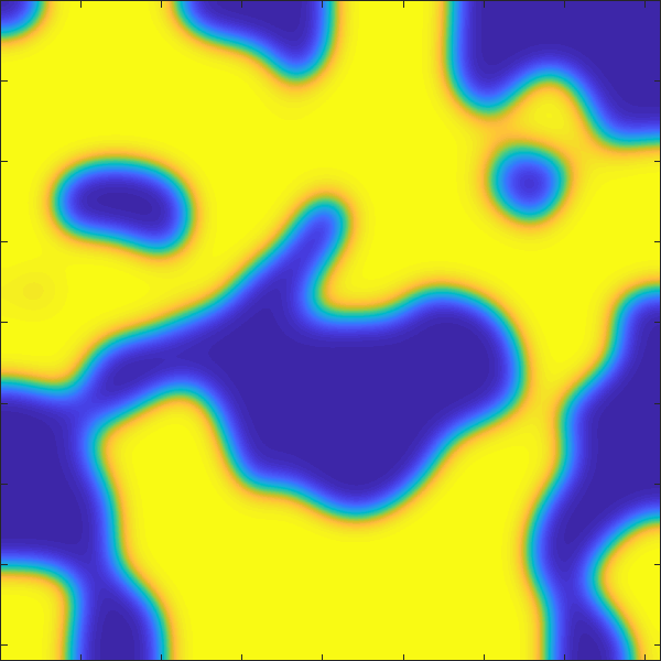
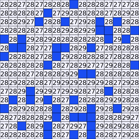
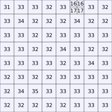
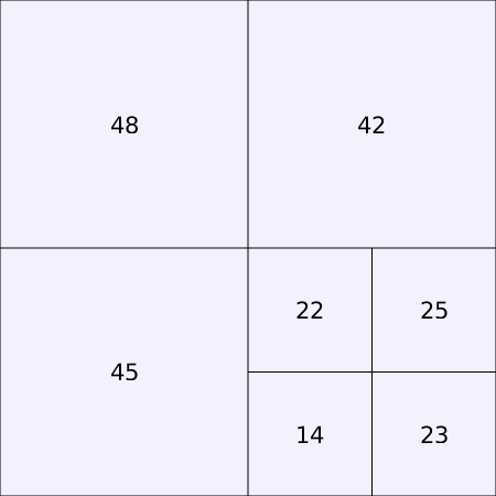
Figure 6: Evolution of the structure and the solution at different time steps.

The initial structure is a tree with a single node labeled as dense, and the HALR representation can be used already at time $0.3$. Then, the solution becomes (numerically) low-rank at time $6.7$ (with rank approximately $50$); the third image in Figure 6 shows the low-rank structure at time $t=18$. Later, as the phase separation happens, the representation becomes again HALR, and stabilizes at the format shown in the fourth figure. The time required for each iteration, and the structure adopted is reported in Figure 7. Analogously to the Burgers’ example, the 1D Laplacian with Neumann boundary conditions can diagonalized via the cosine transform providing a dense method with iteration cost $\mathcal{O}(n^{2}\log(n))$. In the right part of Table 2, we have reported the times required by the dense method for integrating (11) and the average time for solving the Lyapunov equation via fast diagonalization; we see that exploiting the structure makes the HALR approach faster from dimension 16384.

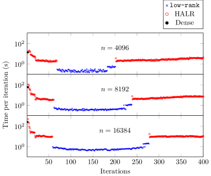
Figure 7: Execution time per iteration for the Allen-Cahn problem. The reported timings are for $\mathsf{maxrank}=50$, and $n=4096$, $n=8192$, and $n=16384$.

$\mathsf{maxrank}=25$ $\mathsf{maxrank}=50$ $n$ $T_{\mathrm{tot}}$ (s) $T_{\mathrm{lyap}}$ (s) $T_{\mathrm{adapt}}$ (s) Mem. $T_{\mathrm{tot}}$ (s) $T_{\mathrm{lyap}}$ (s) $T_{\mathrm{adapt}}$ (s) Mem. $1024$ $277.1$ $153.0$ $124.1$ $8.0$ $317.6$ $197.1$ $120.5$ $8.0$ $2048$ $1080.6$ $733.7$ $346.9$ $32.0$ $713.9$ $561.0$ $152.9$ $32.0$ $4096$ $1754.2$ $1479.8$ $274.4$ $128.0$ $900.7$ $701.5$ $199.2$ $128.0$ $8192$ $3702.4$ $3202.8$ $499.5$ $512.0$ $1823.7$ $1428.9$ $394.7$ $512.0$ $16384$ $7704.5$ $6392.1$ $1312.4$ $2048.0$ $3688.1$ $2765.7$ $922.5$ $2048.0$ $\mathsf{maxrank}=75$ $\mathsf{maxrank}=100$ $n$ $T_{\mathrm{tot}}$ (s) $T_{\mathrm{lyap}}$ (s) $T_{\mathrm{adapt}}$ (s) Mem. $T_{\mathrm{tot}}$ (s) $T_{\mathrm{lyap}}$ (s) $T_{\mathrm{adapt}}$ (s) Mem. $1024$ $229.6$ $151.1$ $78.4$ $8.0$ $\mathbf{187.9}$ $118.9$ $69.0$ $8.0$ $2048$ $430.9$ $338.2$ $92.7$ $32.0$ $\mathbf{346.9}$ $252.0$ $94.9$ $32.0$ $4096$ $619.7$ $444.2$ $175.4$ $128.0$ $\mathbf{505.2}$ $325.6$ $179.6$ $128.0$ $8192$ $1424.5$ $1036.0$ $388.4$ $512.0$ $\mathbf{1147.4}$ $731.0$ $416.3$ $512.0$ $16384$ $2899.1$ $1982.0$ $917.1$ $2048.0$ $\mathbf{2336.8}$ $1331.8$ $1005.0$ $2048.0$

Table 3: Time and storage required for integrating the Allen-Cahn equation from $0$ to $40$, for different values of $n$ and of $\mathsf{maxrank}$. The best times for a given $N$ are reported in bold. The reported memory is measured in Megabytes (MB), and is the maximum memory consumption for storing the solution during the iterations.

4.3 Inhomogeneous Helmholtz equation

Let us consider the following Helmholtz equation with Neumann boundary conditions on the square $\Omega:=[-1,1]^{2}$:

$$\begin{cases}\Delta u+ku+f=0\\ \displaystyle\frac{\partial u}{\partial\vec{n}}=0&\text{on }\partial\Omega\end{cases},\qquad\left\{\begin{array}[]{l}k(x,y):=2500\cdot e^{-50\left|x^{2}+(y+1)^{2}-\frac{1}{4}\right|}\\ f(x,y):=\frac{e^{-x^{2}-y^{2}}}{100}\end{array}\right..$$ (12)

The chosen coefficient $k(x,y)$ is negligible outside of a semi annular region centered in $(0,-1)$; the source term $f$ is concentrated around the origin. The numerical solution of (12), reported in Figure 8, is well approximated in the HALR format which refines the block low rank structure in the region where $k$ takes the larger values.

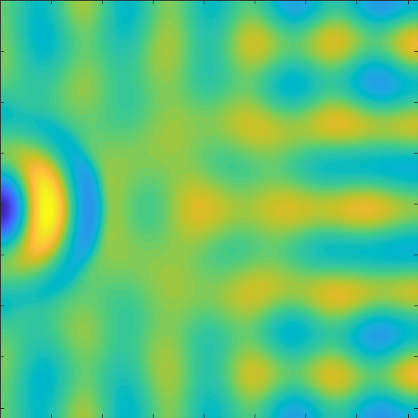
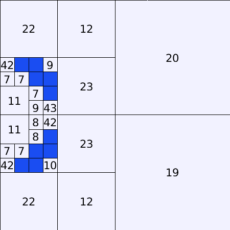
Figure 8: Solution of the Helmholtz equation (12) discretized on a $4096\times 4096$ grid (left) and its representation in the HALR format (right), with $\mathsf{maxrank}=50$.

The usual finite difference discretization of (12) provides the $n^{2}\times n^{2}$ linear system

$$\left(A\otimes I+I\otimes A+D_{k}\right)\mathrm{vec}(X)+\mathrm{vec}(F)=0,$$ (13)

where $A$ is the 1D Laplacian matrix with Neumann boundary conditions, $D_{k}$ is the diagonal matrix containing the evaluations of $k(x,y)$ at the grid points and $F$ contains the analogous evaluations of the source term. Note that, omitting the matrix $D_{k}$, (13) can be solved as a Lyapunov equation. In the spirit of numerical methods for generalized matrix equations [3], we propose to solve (13) with a structured GMRES iteration using the Lyapunov solver as preconditioner; more specifically we store all the (matricized) vectors generated by the GMRES in the HALR format. If necessary (when the rank grows) we adjust the partitioning of the latter via Algorithm 6. The inner product between vectors are computed using the block recursive procedure described in Algorithm 9, which returns the trace of $A^{T}B$ for two HALR matrices $A$ and $B$. Finally, the solution is constructed as a linear combination of HALR matrices. The whole procedure is reported in Algorithm 8.

1:procedure PGMRES($A$, $K$, $F$, $\mathsf{tol}$, $\mathsf{maxrank}$)$\triangleright$ $\operatorname{diag}(\mathrm{vec}(K))=D_{k}$

2:     $B\leftarrow\textsc{Lyap}(A,F)$

3:     $U_{1}\leftarrow B/\lVert B\rVert_{F}$

4:     for $j=1,2,\dots$ do

5:         $R=AU_{j}+U_{j}A^{T}+K\circ U_{j}$

6:         $R\leftarrow\textsc{Repartition}(R,\mathsf{maxrank})$

7:         $W\leftarrow\textsc{Lyap}(A,R)$

8:         for $s=1,\dots,j$ do

9:              $H_{s,j}\leftarrow\textsc{Dot}(W,U_{s})$$\triangleright$ Trace of $W^{T}U_{s}$, see Algorithm 9

10:              $W\leftarrow W-H_{s,j}\cdot U_{s}$

11:         end for

12:         $H_{j+1,j}\leftarrow\lVert W\rVert_{F}$, $U_{j+1}\leftarrow W/\lVert W\rVert_{F}$

13:         $y\leftarrow\lVert B\rVert_{F}H^{\dagger}e_{1}$

14:         if $\lVert Hy-\lVert B\rVert_{F}e_{1}\rVert<\mathsf{tol}\cdot\lVert B\rVert_{F}$ then

15:              break

16:         end if

17:     end for

18:     return $\sum_{j}y_{j}U_{j}$

19:end procedure

Algorithm 8 Structured and preconditioned GMRES iteration for (12)

1:procedure Dot($A$, $B$)

2:     if $A$ and $B$ are leaf nodes or at least one is low-rank then

3:         return $\mathrm{Trace}(A^{T}B)$$\triangleright$ Exploiting the low-rank structure of $A$ or $B$, if any

4:     else

5:         if $A$ is dense or $B$ is dense then

6:              Set the partitioning of $A$ and $B$ equal to the finest of the two.

7:         end if

8:         return Dot($A_{11},B_{11}$) + Dot($A_{12},B_{12}$)+Dot($A_{21},B_{21}$)+Dot($A_{22},B_{22}$)

9:     end if

10:end procedure

Algorithm 9 Trace inner product for two HALR matrices

Equation (12) has been solved for different grid sizes with $\mathsf{maxrank}=50$. The time and memory consumption are reported in Table 4. The storage needed for the solution scales linearly with $n$. In addition, the table contains the number of iterations needed by the preconditioned GMRES to reach the relative tolerance $\mathsf{tol}=10^{-4}$. We note that the number of iterations grows very slowly as the grid size increases. The time required depends on many factors, such as the distribution of the ranks and the complexity of the structure in the basis generated by the GMRES; we just remark that it grows subquadratically for this example. In future work we plan to explore the use of restarting mechanisms and other truncation strategies in order to optimize the approach.

$\mathsf{maxrank}=50$ $n$ $T_{\mathrm{tot}}$ (s) $T_{\mathrm{lyap}}$ (s) $T_{\mathrm{adapt}}$ (s) It. Mem. $1024$ $72.83$ $42.82$ $11.39$ $25$ $1.72$ $2048$ $231.92$ $161.35$ $24.25$ $26$ $3.73$ $4096$ $603.03$ $362.22$ $75.74$ $26$ $8.18$ $8192$ $1773.6$ $982.37$ $244.54$ $26$ $16.68$ $16384$ $5884$ $3065$ $1044.4$ $28$ $33.3$

Table 4: Time and storage required for solving the inhomogeneous Helmholtz equation (12), for different values of $n$ and $\mathsf{maxrank}=50$. The reported memory is measured in Megabytes (MB), and refers to the storage of the solution.

5 Conclusions

In this work, we have proposed a new format for storing matrices arising from 2D discretization of functions which are smooth almost everywhere, with localized singularities. Low-rank decompositions, which are effective for globally smooth functions, become ineffective in this case. The proposed structure automatically adapts to the matrix, and requires no prior information on the location of the singular region. The storage and complexity interpolates between dense and low-rank matrices, based on the structure, with these two cases as extrema.

We demonstrated techniques for the efficient adaptation of the structure in case of moving singularities, with the aim of tracking time-evolution of 2D PDEs; the examples show that the proposed techniques can effectively detect changes in the structure, and ensure the desired level of accuracy. We developed efficient Lyapunov and Sylvester solvers for matrix equations with HALR right-hand-side and HODLR coefficients. This case is of particular interest, as it often arises in discretized PDEs. Several numerical experiments demonstrate both the effectiveness and the flexibility of the approach.

The proposed format may be generalized to discretization of 3D functions by swapping quadtrees with octrees, making the necessary adjustments, and choosing a suitable low-rank format for the blocks. Similar ideas to the ones presented in this work may be used to detect the hierarchical structure in an adaptive way, and to adjust the structure in time. However, devising an efficient Sylvester solver remains challenging. Despite the existence of low-rank solvers for linear systems with Kronecker structure in the Tucker format [16] exploiting the hierarchical structure introduces major difficulties, which we plan to investigate in future work.

References

- [1] Uri M Ascher, Steven J Ruuth, and Raymond J Spiteri. Implicit-explicit Runge-Kutta methods for time-dependent partial differential equations. Applied Numerical Mathematics, 25(2-3):151–167, 1997.
- [2] Mario Bebendorf. Approximation of boundary element matrices. Numerische Mathematik, 86(4):565–589, 2000.
- [3] Peter Benner and Tobias Breiten. Low rank methods for a class of generalized lyapunov equations and related issues. Numerische Mathematik, 124(3):441–470, 2013.
- [4] Peter Benner, Ren-Cang Li, and Ninoslav Truhar. On the ADI method for Sylvester equations. Journal of Computational and Applied Mathematics, 233(4):1035–1045, 2009.
- [5] Steffen Börm. Data-sparse approximation of non-local operator by -matrices. Linear Algebra Appl., 422(2-3):380–403, 2007.
- [6] Kevin Burrage, Nicholas Hale, and David Kay. An efficient implicit fem scheme for fractional-in-space reaction-diffusion equations. SIAM Journal on Scientific Computing, 34(4):A2145–A2172, 2012.
- [7] Vladimir Druskin, Leonid Knizhnerman, and Valeria Simoncini. Analysis of the rational Krylov subspace and ADI methods for solving the lyapunov equation. SIAM Journal on Numerical Analysis, 49(5):1875–1898, 2011.
- [8] Virginie Ehrlacher, Laura Grigori, Damiano Lombardi, and Hao Song. Adaptive hierarchical subtensor partitioning for tensor compression. SIAM Journal on Scientific Computing, 43(1):A139–A163, 2021.
- [9] Lars Grasedyck. Existence of a low rank or -matrix approximant to the solution of a Sylvester equation. Numerical Linear Algebra with Applications, 11(4):371–389, 2004.
- [10] W. Hackbusch, B. N. Khoromskij, and R. Kriemann. Hierarchical matrices based on a weak admissibility criterion. Computing, 73(3):207–243, 2004.
- [11] Wolfgang Hackbusch. Hierarchical matrices: algorithms and analysis, volume 49 of Springer Series in Computational Mathematics. Springer, Heidelberg, 2015.
- [12] Nathan Halko, Per-Gunnar Martinsson, and Joel A Tropp. Finding structure with randomness: Probabilistic algorithms for constructing approximate matrix decompositions. SIAM review, 53(2):217–288, 2011.
- [13] I. Jonsson and B. Kågström. Recursive blocked algorithm for solving triangular systems. I. One-sided and coupled Sylvester-type matrix equations. ACM Trans. Math. Software, 28(4):392–415, 2002.
- [14] Vladimir Kazeev and Christoph Schwab. Quantized tensor-structured finite elements for second-order elliptic PDEs in two dimensions. Numer. Math., 138(1):133–190, 2018.
- [15] Daniel Kressner, Stefano Massei, and Leonardo Robol. Low-rank updates and a divide-and-conquer method for linear matrix equations. SIAM Journal on Scientific Computing, 41(2):A848–A876, 2019.
- [16] Daniel Kressner and Christine Tobler. Low-rank tensor krylov subspace methods for parametrized linear systems. SIAM Journal on Matrix Analysis and Applications, 32(4):1288–1316, 2011.
- [17] Wenyuan Liao. A fourth-order finite-difference method for solving the system of two-dimensional Burgers’ equations. Internat. J. Numer. Methods Fluids, 64(5):565–590, 2010.
- [18] Stefano Massei, Davide Palitta, and Leonardo Robol. Solving rank-structured sylvester and lyapunov equations. SIAM Journal on Matrix Analysis and Applications, 39(4):1564–1590, 2018.
- [19] Stefano Massei, Leonardo Robol, and Daniel Kressner. hm-toolbox: Matlab software for HODLR and HSS matrices. SIAM Journal on Scientific Computing, 42(2):C43–C68, 2020.
- [20] Davide Palitta and Valeria Simoncini. Matrix-equation-based strategies for convection–diffusion equations. BIT Numerical Mathematics, 56(2):751–776, 2016.
- [21] Horst D Simon and Hongyuan Zha. Low-rank matrix approximation using the Lanczos bidiagonalization process with applications. SIAM Journal on Scientific Computing, 21(6):2257–2274, 2000.
- [22] V. Simoncini. A new iterative method for solving large-scale Lyapunov matrix equations. SIAM J. Sci. Comput., 29(3):1268–1288, 2007.
- [23] V. Simoncini. Computational methods for linear matrix equations. SIAM Rev., 58(3):377–441, 2016.
- [24] Alex Townsend and Sheehan Olver. The automatic solution of partial differential equations using a global spectral method. Journal of Computational Physics, 299:106–123, 2015.
- [25] Eugene Tyrtyshnikov. Incomplete cross approximation in the mosaic-skeleton method. Computing, 64(4):367–380, 2000.
- [26] Jianlin Xia, Shivkumar Chandrasekaran, Ming Gu, and Xiaoye S Li. Fast algorithms for hierarchically semiseparable matrices. Numerical Linear Algebra with Applications, 17(6):953–976, 2010.