Regularized Nonlinear Regression for Simultaneously Selecting and Estimating Key Model Parameters

Abstract

In system identification, estimating parameters of a model using limited observations results in poor identifiability. To cope with this issue, we propose a new method to simultaneously select and estimate sensitive parameters as key model parameters and fix the remaining parameters to a set of typical values. Our method is formulated as a nonlinear least squares estimator with $L_{1}$-regularization on the deviation of parameters from a set of typical values. First, we provide consistency and oracle properties of the proposed estimator as a theoretical foundation. Second, we provide a novel approach based on Levenberg-Marquardt optimization to numerically find the solution to the formulated problem. Third, to show the effectiveness, we present an application identifying a biomechanical parametric model of a head position tracking task for 10 human subjects from limited data. In a simulation study, we analyze the bias and variance of estimated parameters. In an experimental study, our method improves the model interpretation by reducing the number of parameters to be estimated while maintaining variance accounted for (VAF) at above 82.5$\%$. Moreover, the variance of estimated parameters is reduced by 71.1$\%$ as compared to that of the estimated parameters without ${L}_{1}$-regularization. Our method is 54 times faster than the standard simplex-based optimization to solve the regularized nonlinear regression.

1 Introduction

In parameter estimation, a model is considered to be identifiable when a unique set of parameters is specified for given measurement data. However, when the data is limited, estimating unknown parameters of a model results in poor identifiability gutenkunst2007universally . In such a case, small changes in the data could result in very different estimated parameters, for example, a rather randomly chosen local minimum out of multiple local minima lund2019global ; ramadan2018selecting . The resulted overfitting impairs the model parsimony and generalizability pitt2002good . The overfitted model may yield good results with a training data set used to estimate parameters, but it may yield poor estimates with a new test data set. Moreover, this issue becomes worse when parameters are estimated from the data corrupted by random noise geman1992neural.

A biomechanical model often has unknown parameters to be estimated with limited data due to unavailable internal states and the non-invasive nature of human data collection little2010parameter . For a limited observation data set, one way for improving identifiability is to build a parsimonious model by lumping a large number of parameters into a small number of lumped parameters do2018appearance . Such a parsimonious model has better interpretability and provides higher estimation accuracy for arbitrary data babyak2004you .

As a way to build a parsimonious model, the Least absolute shrinkage and selection operator (Lasso) was first introduced in tibshirani1996regression and then further developed in zou2005regularization ; tibshirani2005sparsity ; yuan2006model ; zou2006adaptive . The Lasso is typically used to select sensitive parameters among parameters of a linear model. A sensitive parameter subset is considered to have relatively large impact on the output of the model. That is, small changes in the sensitive parameters result in large changes in the model response tibshirani1988sensitive .

To formally introduce the Lasso, we suppose that we have $(\bm{x}_{i},y_{i}),i\in\{1,\cdots,n\}$ where $\bm{x}_{i}=[x_{i}^{[1]},\cdots,x_{i}^{[p]}]$ and $y_{i}=f({\bm{x}_{i}};\bm{\theta}_{0})+\epsilon_{i}$. $f({\bm{x}_{i}};\bm{\theta}_{0})$ is a function, which depends on the true parameter vector $\bm{\theta}_{0}$. $\epsilon_{i}$ is independent and identically distributed with $\mathbb{E}(\epsilon)=0$ and $Var(\epsilon_{i})=\sigma^{2}$. Without loss of generality, we assume that the true parameter vector $\bm{\theta}_{0}=[\theta_{01},\theta_{02},...,\theta_{0s},\theta_{0s+1},...,\theta_{0p}]^{T}$ has the first $s$ entries non-zero. That is, $\theta_{0k}\neq 0$, for $1\leq k\leq s$ and $\theta_{0k}=0$, for $s+1\leq k\leq p$. Finally, when $f({\bm{x}_{i}};\bm{\theta}_{0})={\bm{x}_{i}\bm{\theta}_{0}}$, we consider the following linear least squares problem with $L_{1}$-regularization.

$$\hat{\bm{\theta}} =\arg\min\limits_{\theta}\left[\|\bm{y}-\bm{X}\bm{\theta}\|^{2}_{2}+n\lambda\sum_{k=1}^{p}|\theta_{k}|\right],$$ (1)

where $\bm{X}=[\bm{x}_{1},\bm{x}_{2},\cdots,\bm{x}_{n}]\in\mathbb{R}^{n\times p}$ is the input. $\bm{y}=[y_{1},y_{2},\cdots,y_{n}]^{T}\in\mathbb{R}^{n\times 1}$ is the observation vector. In (1), the hyperparameter $\lambda>0\in\mathbb{R}$ determines the amount of regularization. The Lasso shrinks more number of parameters toward 0 as $\lambda$ increases in general. Moreover, insensitive parameters are shrunk to 0 if $\lambda$ is sufficiently large zou2006adaptive . The remaining parameters, which are not shrunk to 0, are considered sensitive parameters ramadan2018selecting . In this paper, we consider the sensitive parameters as key model parameters. The ${L}_{1}$-regularization methods and weighted least squares method were used to select nonlinear auto regressive with exogenous variables (NARX) models qin2012selection . The Lasso was used to remove insensitive parameters when all unknown parameters are to be non-negative kump2012variable . The modified Lasso was proposed for the nonlinear induction motor identification problem, which deals with a similar problem to our study rasouli2012reducing . However, they do not provide consistency and the asymptotic normality results. The modified principal component analysis (PCA) based on the Lasso was proposed for dimension reduction jolliffe2003modified . To select and estimate sensitive parameters of a model, sensitive parameters were selected based on parameter estimation variances predicted by the Fisher information matrix ramadan2018selecting ; ramadan2019feasibility .

In this paper, our objective is to develop a regularized nonlinear parameter estimation method for a model with unknown parameters using a limited data set. Thus, we formulate the model parameter estimation problem as a nonlinear least squares problem with $L_{1}$-regularization as follows.

$$\hat{\tilde{\bm{\theta}}}= \arg\min\limits_{{\tilde{\bm{\theta}}}}\left[\|\bm{y}-{f}(\bm{X};\tilde{\bm{\theta}})\|^{2}_{2}+n\lambda\sum_{k=1}^{p}|\tilde{\theta}_{k}|\right],$$ (2)

where ${\tilde{\bm{\theta}}}:=\bm{\theta}-{\bar{\bm{\theta}}}$ and ${\bar{\bm{\theta}}}$ is the set of typical values. Note that these values may be obtained as the mean values of $\bm{\theta}$ based on preliminary information or estimation. The details of (2) are introduced in Section 3. In our preliminary work, we developed a parameter selection method for system identification with application to head-neck position tracking and reported the model parameter estimates kyubaek2019penalized .

The contributions of the paper are as follows. First, we consider nonlinear regression with a generalized penalty function that includes an ${L}_{1}$-penalty function and provide its consistency and oracle properties (i.e., convergence to the correct sparsity and asymptotic normality) in Section 2. To the best of the authors’ knowledge, our work is the first to provide such analysis for nonlinear regression with a generalized penalty function. For example, convergence properties for various penalized linear regression have been discussed johnson2008penalized ; fan2001scad . Note that we do not assume the distribution of errors, which is different from the assumption of fan2001scad . In Section 3, we then reformulate the regularized nonlinear regression for simultaneously selecting and estimating key model parameters by defining $\tilde{\theta}_{k}$ in (2) as the deviation of the k-th parameter from its nominal value. Next, we improve the optimization algorithm of rasouli2012reducing to numerically solve the nonlinear least squares problem. Finally, to show the effectiveness, we present an application identifying a biomechanical parametric model of a head-neck position tracking task from limited data in simulation and experimental studies. In a simulation study, our algorithm reduces the variance of most parameter estimates as well as the bias. In an experimental study, the variance of selected sensitive parameters is reduced by $71.1\%$ on average while maintaining the goodness of fit at above $82.5\%$. In addition, our method is 54 times faster as compared to the Lasso with the brute force optimization, e.g., the standard simplex-based optimization we presented recently ramadan2018selecting .

2 Consistency and Oracle Properties

We propose a penalized nonlinear regression approach for parameter selection and estimation. First of all, we adopt the following equivalent nonlinear least squares estimator with a generalized penalty function from (2):

$$\hat{\bm{\theta}}_{n}=\arg\min_{\bm{\theta}\in D}\left[\bm{Q}_{n}(\bm{\theta}):=\bm{S}_{n}(\bm{\theta})+n\sum^{p}_{k=1}p_{\lambda_{n}}(|\theta_{k}|)\right],$$ (3)

where $\bm{S}_{n}(\bm{\theta})=\sum^{n}_{i=1}\left(y_{i}-f({\bm{x}_{i}};\bm{\theta})\right)^{2}$. The first term in $\bm{Q}_{n}(\cdot)$ corresponds to nonlinear least squares estimation, and the second term, $p_{\lambda_{n}}(\cdot)$ is the penalty function used for parameter selection. $\lambda_{n}$ in the penalty function is a nonnegative regularization parameter. Note that we consider a generalized penalty function in (3). The appropriate choice of the penalty function, including $L_{1}$-regularization, is further investigated in the assumption  2.

Without loss of generality, we assume only a few parameters are non-zero, such that the true parameter vector $\bm{\theta}_{0}=[\theta_{01},\theta_{02},...,\theta_{0s},\theta_{0s+1},...,\theta_{0p}]$ has the first $s$ entries non-zero. That is, $\theta_{0k}\neq 0$, for $1\leq k\leq s$ and $\theta_{0k}=0$, for $s+1\leq k\leq p$. For the nonlinear function $f(\cdot;\cdot)$ in (3), we further consider the following assumptions.

Assumption 1

(Nonlinear function)

1. The true parameter $\bm{\theta}_{0}$ is in the interior of the bounded parameter set $\Theta$, and $f({\bm{x}_{i}};\bm{\theta})$ is twice differentiable with respect to $\bm{\theta}$ near $\bm{\theta}_{0}$ for all $i$.

2. Let $\bm{f}_{k}(\bm{\theta})=\left(\frac{\partial{f(\bm{x}_{1},\bm{\theta})}}{\partial\theta_{k}},\ldots,\frac{\partial f(\bm{x}_{n},\bm{\theta})}{\partial\theta_{k}}\right)^{T}$ and ${\bm{\dot{F}}}(\bm{\theta})=(\bm{f}_{1},...,\bm{f}_{p})$. Then, there exists a positive definite matrix $\Gamma$ such that $\frac{1}{n}{\bm{\dot{F}}}(\bm{\theta}_{0})^{T}{\bm{\dot{F}}}(\bm{\theta}_{0})\rightarrow\Gamma$ as $n\rightarrow\infty$.

3. As $n\rightarrow\infty$ and $\|\bm{\theta}_{1}-\bm{\theta}_{0}\|\rightarrow 0$,

   $${\bm{\dot{F}}}(\bm{\theta}_{1})^{T}{\bm{\dot{F}}}(\bm{\theta}_{1})\left({\bm{\dot{F}}}(\bm{\theta}_{0})^{T}{\bm{\dot{F}}}(\bm{\theta}_{0})\right)^{-1}\rightarrow I$$

   uniformly, where $I$ is the identity matrix

4. There exists a $\delta>0$ such that

   $$\limsup_{n\rightarrow\infty}\frac{1}{n}\sum^{n}_{i=1}\sup_{\|\bm{\theta}-\bm{\theta}_{0}\|\leq\delta}\left(\frac{\partial^{2}f(\bm{x}_{i};\bm{\theta})}{\partial\theta_{k}\partial\theta_{s}}\right)^{2}<\infty$$

For the penalty function $p_{\lambda_{n}}(\cdot)$ in (3), we further consider the following assumptions.

Assumption 2

(Penalty function) The first and second derivative of the penalty function $p_{\lambda_{n}}(\cdot)$ denoted by $q_{\lambda_{n}}(\cdot)$ and $q^{\prime}_{\lambda_{n}}(\cdot)$ have the following properties:

1. For a nonzero fixed $\theta$,

   $$\lim_{n\to\infty}n^{1/2}q_{\lambda_{n}}(|\theta|)=0,\lim_{n\to\infty}q^{\prime}_{\lambda_{n}}(|\theta|)=0.$$

2. For any $M>0$,

   $$\lim_{n\to\infty}n^{1/2}\inf_{|\theta|\leq Mn^{-1/2}}q_{\lambda_{n}}(|\theta|)\rightarrow\infty.$$

Remark 1

Assumption 2 is satisfied for several well known penalty functions, e.g., SCAD, Adaptive Lasso, and Hard penalty with proper choices of $\lambda_{n}$. Assumption 2-(1) is satisfied for $L_{1}$-regularization with a proper choice of $\lambda_{n}$. The details are discussed in johnson2008penalized .

The following theorem shows the existence of a local minimizer of $\bm{Q}_{n}(\bm{\theta})$ with the order of $O_{p}(n^{-1/2})$.

Lemma 1

Under Assumptions 1 and 2-(1), for any $\eta>0$, there exists a positive constant $C$ that makes, for large enough n,

$$P\left(\inf_{\|\bm{v}\|=C}\bm{Q}_{n}(\bm{\theta}_{0}+n^{-1/2}\bm{v})-\bm{Q}_{n}(\bm{\theta}_{0})>0\right)>1-\eta,$$

where $\bm{Q}_{n}(\bm{\theta})=\bm{S}_{n}(\bm{\theta})+n\sum^{p}_{k=1}p_{\lambda_{n}}(|\theta_{k}|)$.

Theorem 1

Under the assumptions in Lemma 1, there exists, with probability tending to 1, a root-n-consistent local minimizer $\hat{\bm{\theta}}$ of $\bm{Q}_{n}(\bm{\theta})$, that is, $\|\hat{\bm{\theta}}-\bm{\theta}_{0}\|=O_{p}(n^{-1/2})$.

Next theorem shows oracle properties (i.e., convergence to the correct sparsity and asymptotic normality) of the estimator on the true set.

Theorem 2

Assume that $\hat{\bm{\theta}}=(\hat{\theta}_{k})^{p}_{k=1}$ is the local minimizer of $\bm{Q}_{n}(\bm{\theta})$ with the root-n-consistency. If Assumptions 1 and 2 hold,

• for the set $M_{k}=\{\omega:\hat{\theta}_{k}\neq 0\}$,  $s+1\leq k\leq p$,

  $$P(M_{k})~{}\rightarrow~{}0$$

• For $\hat{\bm{\theta}}_{11}=(\hat{\theta}_{1},\hat{\theta}_{2},...,\hat{\theta}_{s})^{T}$, ${\bm{\theta}}_{01}=({\theta}_{01},{\theta}_{02},...,{\theta}_{0s})^{T}$,

  $$n^{1/2}(2\Gamma_{11})({\hat{\bm{\theta}}}_{11}-\bm{\theta}_{01}+(2\Gamma_{11})^{-1}b_{n})~{}\stackrel{{\scriptstyle d}}{{\longrightarrow}}~{}N(0,2\Gamma_{11}\sigma^{2}),$$

  where $b_{n}=(q_{\lambda_{n}}({|\theta_{01}|)\text{sgn}(\theta}_{01}),q_{\lambda_{n}}({|\theta_{02}|)\text{sgn}(\theta}_{02}),...$, $q_{\lambda_{n}}(|\theta_{0s}|)\text{sgn}(\theta_{0s}))^{T}$ and $\Gamma_{11}$ is the first $s\times s$ submatrix of $\Gamma$.

The proofs of Lemma 1 and Theorem 1 are given in Appendix A and Appendix B, respectively and the proof of Theorem 2 is given in Appendix C.

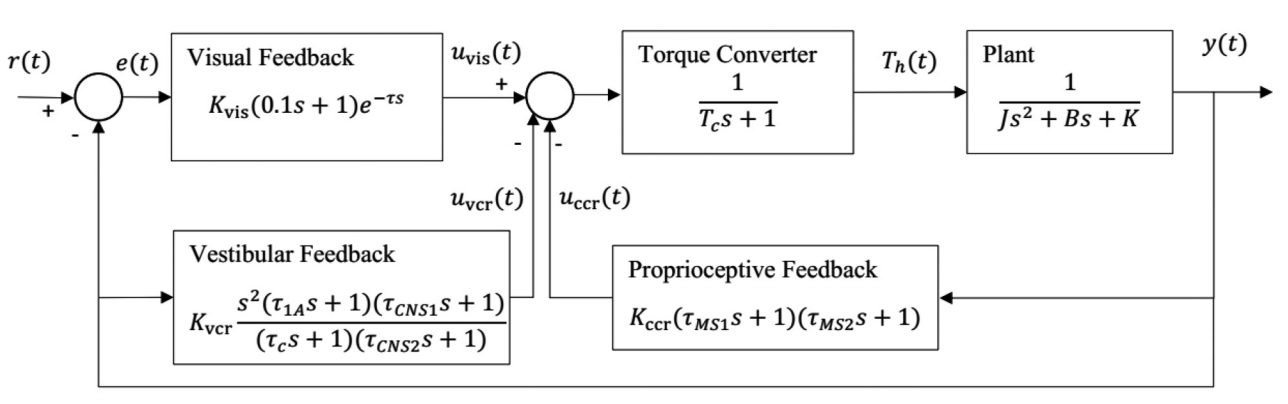
Figure 1: Sensorimotor control block diagram for the head-neck system ramadan2018selecting

3 Application to Head Position Tracking

In this section, we evaluate our approach to solve the nonlinear least squares problem with $L_{1}$-regularization from simulation and experimental studies of a biomechanical parametric model of a head-neck position tracking task in ramadan2018selecting . The reliability of the head-neck position tracking task to quantify head-neck motor control is demonstrated in popovich2015quantitative . As compared to the Levenberg optimization algorithm in rasouli2012reducing , our method implements the Levenberg-Marquardt optimization algorithm to numerically solve our nonlinear least squares problem with $L_{1}$-regularization. The Levenberg-Marquardt optimization uses the diagonal elements of the hessian matrix approximation to overcome the slow convergence problem when the value of the damping factor is large more1978levenberg . The details of our algorithm are shown in Appendix D and Table 3.

Additionally, in order to simultaneously select and estimate key model parameters of the head-neck system, we reformulate the Lasso penalty function as ${L}_{1}$-regularization on the deviation of parameters from a set of typical values. In this paper, we adopt the mean of the nominal parameter values obtained from preliminary estimation as the set of typical values. Therefore, our method simultaneously selects and estimates only sensitive parameters while fixing insensitive parameters onto the mean of the nominal parameter values. In order to compare with the method of ramadan2018selecting , we set the number of sensitive parameters to 5. In this case, we increase the regularization hyperparameter value until we obtain 5 sensitive parameters. The goodness of fit is quantitatively evaluated by variance accounted for (VAF). VAF represents how much the experimental data can be explained by a fitted regression model. VAF is formally defined as follows.

$${\text{VAF}}(\bm{\theta})(\%)=\left[1-\frac{\sum^{n}_{i=1}(y_{i}-\hat{y}_{i}(\bm{\theta}))^{2}}{\sum^{n}_{i=1}y_{i}^{2}}\right]\times 100$$

Table 1: The neurophysiological parameters of the head position model. All the information is obtained from ramadan2018selecting

Parameters		Max	Min	Description
$\bm{\theta}$	$K_{vis}[\frac{Nm}{rad}]$	$10^{3}$	50	Visual feedback gain
	$K_{vcr}[\frac{Nms^{2}}{rad}]$	$10^{4}$	500	Vestibular feedback gain
	$K_{ccr}[\frac{Nm}{rad}]$	300	1	Proprioceptive feedback gain
	$\tau[s]$	0.4	0.1	Visual feedback delay
	$\tau_{1A}[s]$	0.2	0.01	Lead time constant of the irregular vestibular afferent neurons
	$\tau_{CNS1}[s]$	1	0.05	Lead time constant of the central nervous system
	$\tau_{C}[s]$	5	0.1	Lag time constant of the irregular vestibular afferent neurons
	$\tau_{CNS2}[s]$	60	5	Lag time constant of the central nervous system
	$\tau_{MS1}[s]$	1	0.01	First lead time constant of the neck muscle spindle
	$\tau_{MS2}[s]$	1	0.01	Second lead time constant of the neck muscle spindle
	$B[\frac{Nm}{rad}]$	5	0.1	Intrinsic damping
	$K[\frac{Nm}{rad}]$	5	0.1	Intrinsic stiffness
$\bm{\theta_{fixed}}$	$J[kgm^{2}]$	0.0148	0.0148	Head inertia
	$T_{c}[s]$	0.1	0.1	Torque converter time constant

3.1 Subjects

10 healthy subjects participated in the experimental study. They did not have any history of neck pain lasting more than three days or any neurological motor control impairments. The Michigan State University’s Biomedical and Health Institutional Review Board approved the test protocol. The subjects signed an informed consent before participating in the experiment ramadan2018selecting ; ramadan2019feasibility .

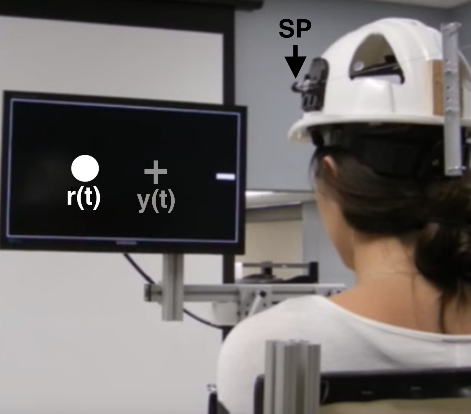
Figure 2: The experimental setup for the head-neck position tracking task. $r(t)$ is the reference command signal, and $y(t)$ is the measured head rotation angle, and SP indicates one of string potentiometers on both sides of the helmet.

3.2 Parametric model

Fig. 1 shows the block diagram of the head-neck system for position tracking. This is a representative physiological feedback control model peng1996dynamical ; chen2002modeling . The model consists of 14 parameters. As shown in Table 1, 2 out of 14 parameters are set to fixed values from peng1996dynamical . The remaining 12 parameters to be estimated are:

$$\begin{split}\bm{\theta}=[{K}_{vis}\ {K}_{vcr}\ {K}_{ccr}\ \tau\ \tau_{1A}\ \tau_{CNS1}\\ \tau_{C}\ \tau_{CNS2}\ \tau_{MS1}\ \tau_{MS2}\ {B}\ {K}]\end{split}$$

The remaining 12 parameters have the lower and upper bounds from ramadan2018selecting and are normalized using min-max normalization in order to ignore the scale differences between parameters.

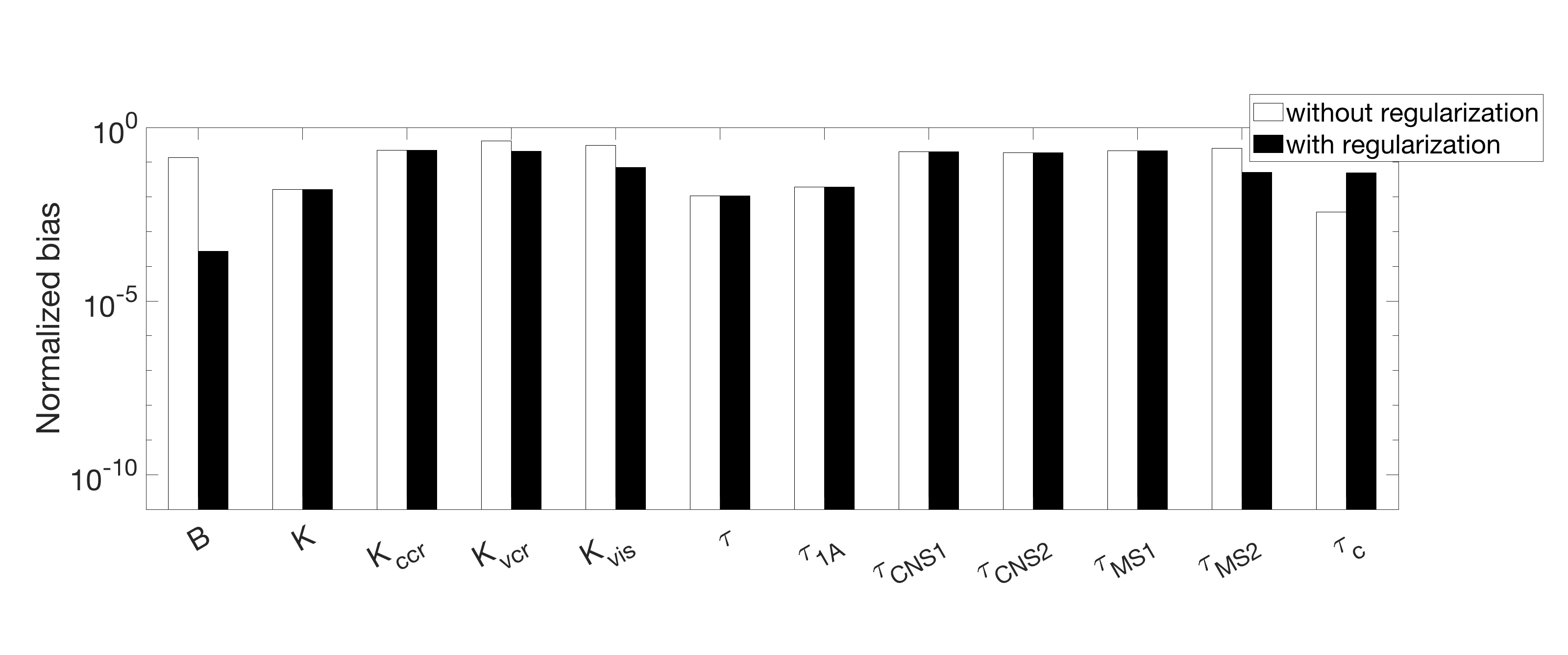
(a)

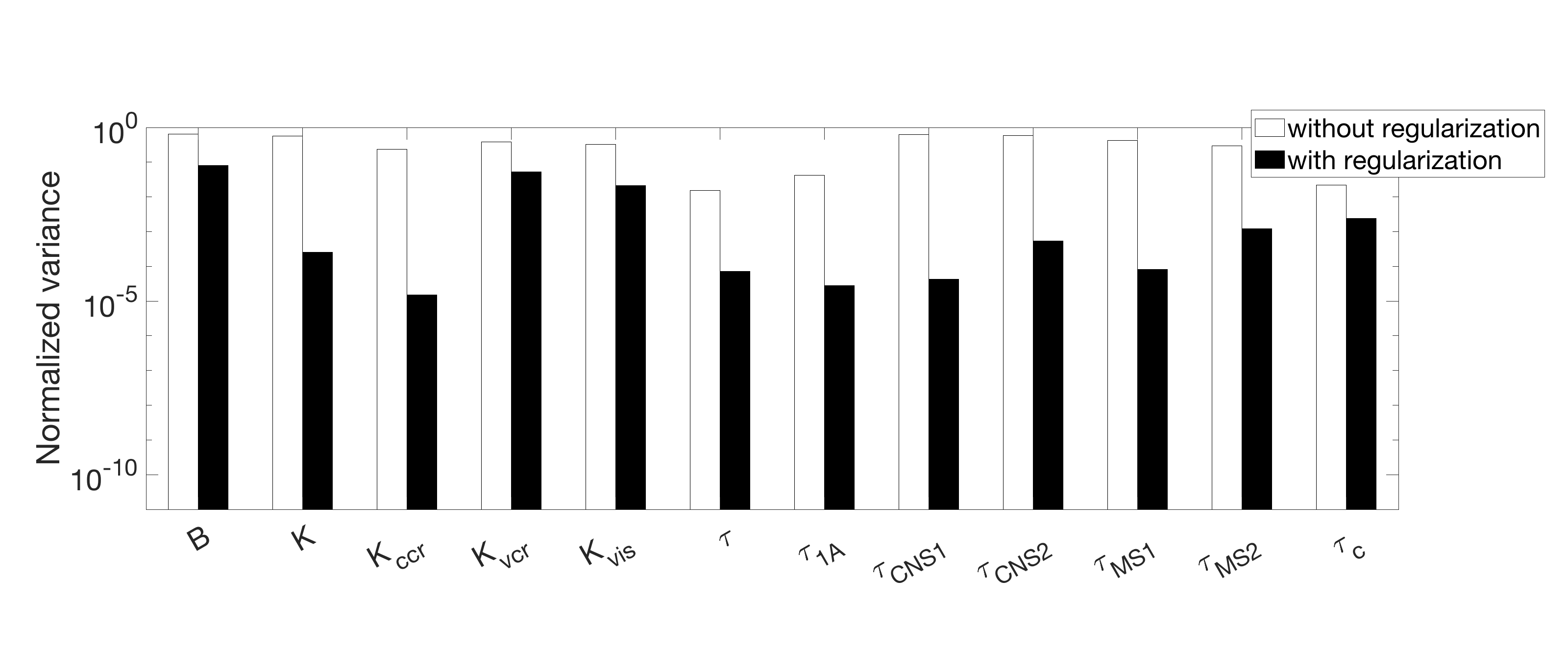
(b)

Figure 3: The bias (a) and variance (b) of estimated parameters in the simulation studies. Comparing our method with a nonlinear least squares problem without ${L}_{1}$-regularization (white bar), we set the mean of nominal parameters (black bar) obtained from preliminary estimation as a set of typical values. The y-axis is a logarithmic scale.

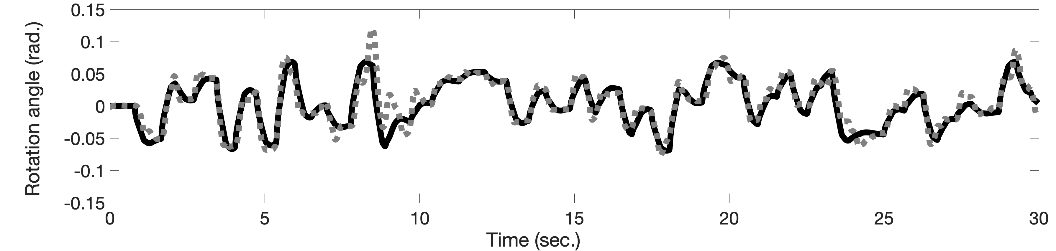
(a) Subject 1

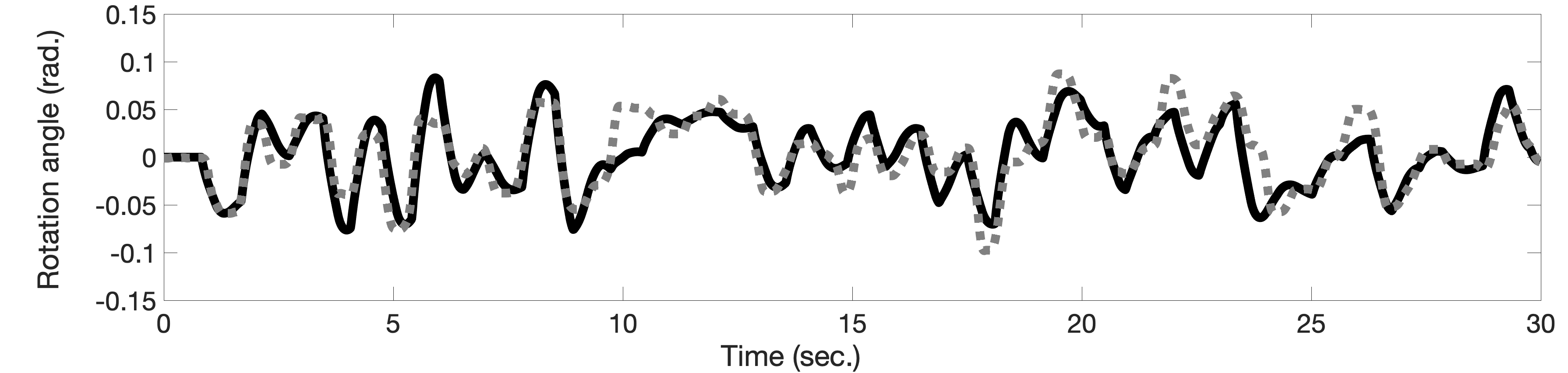
(b) Subject 2

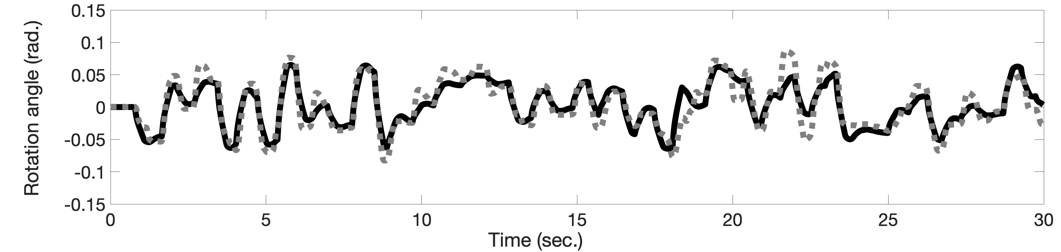
(c) Subject 3

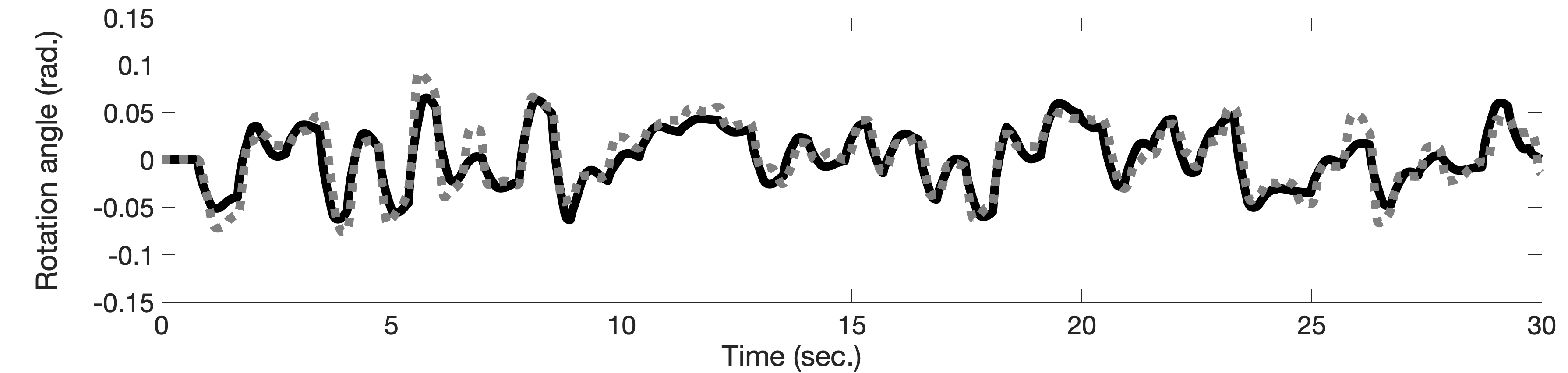
(d) Subject 4

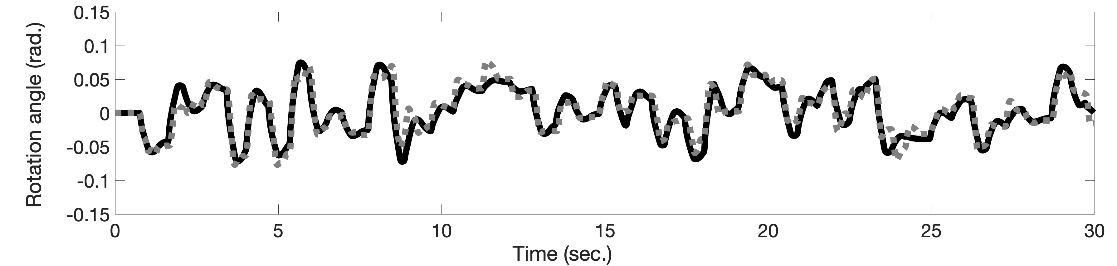
(e) Subject 5

Figure 4: The curve fitting with 10 experimental cases. Solid lines represent estimated responses from the fitted models and dotted lines represent measured responses.

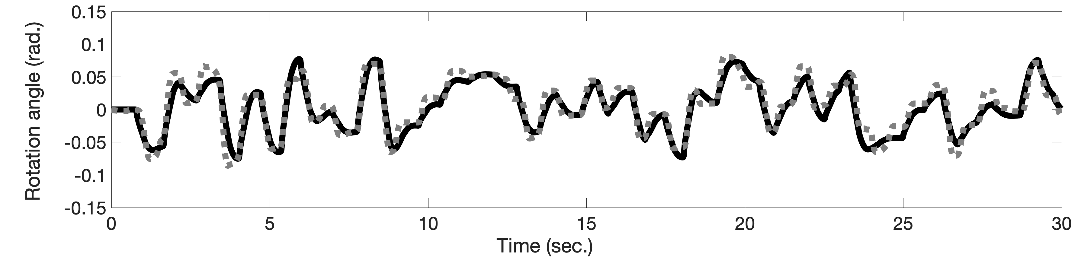
(f) Subject 6

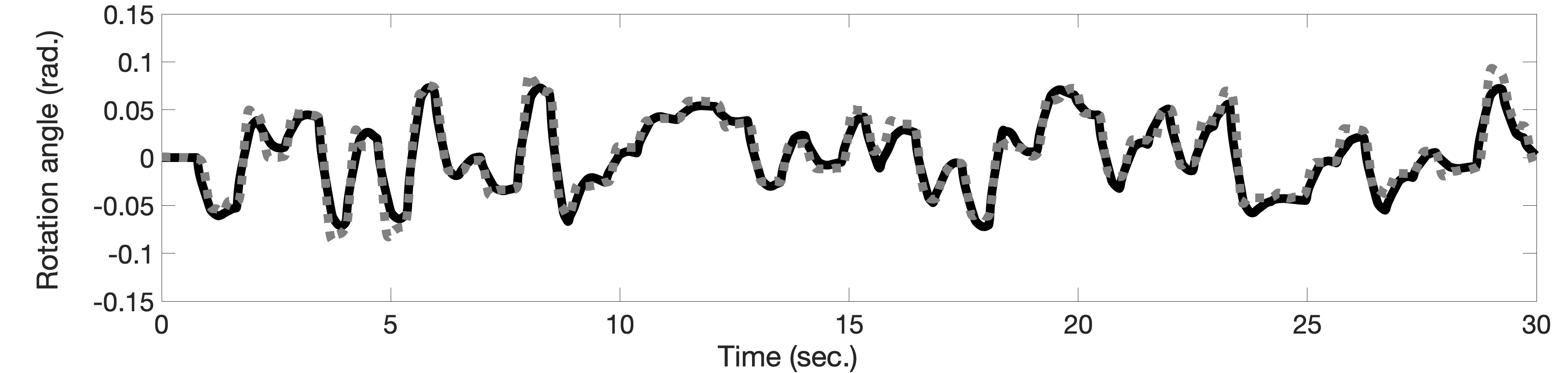
(g) Subject 7

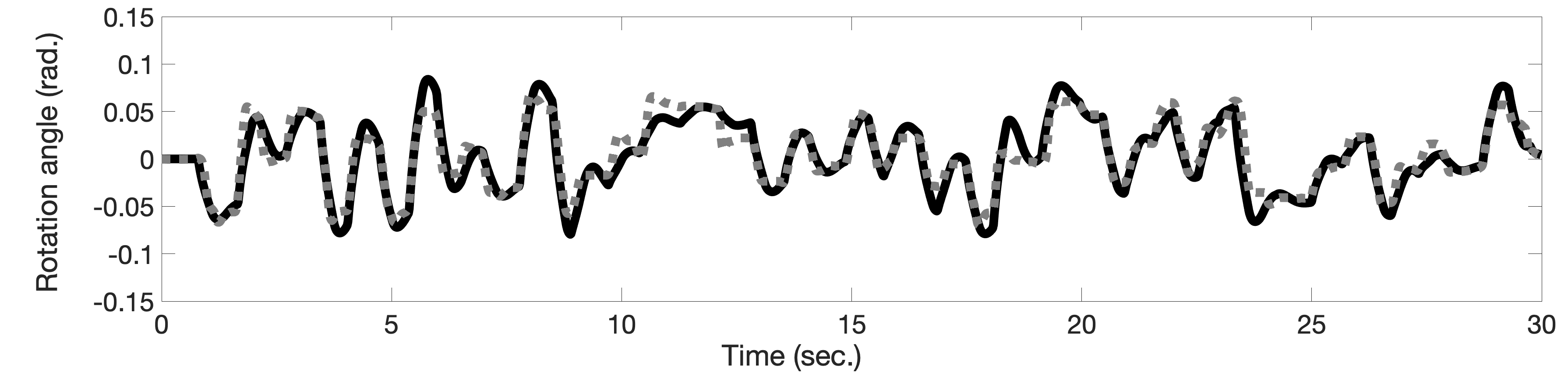
(h) Subject 8

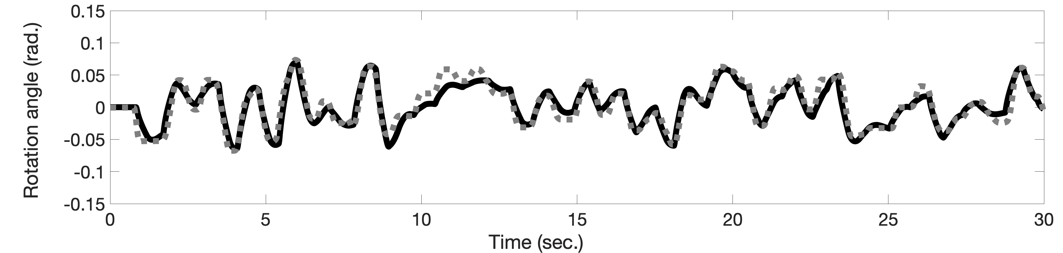
(i) Subject 9

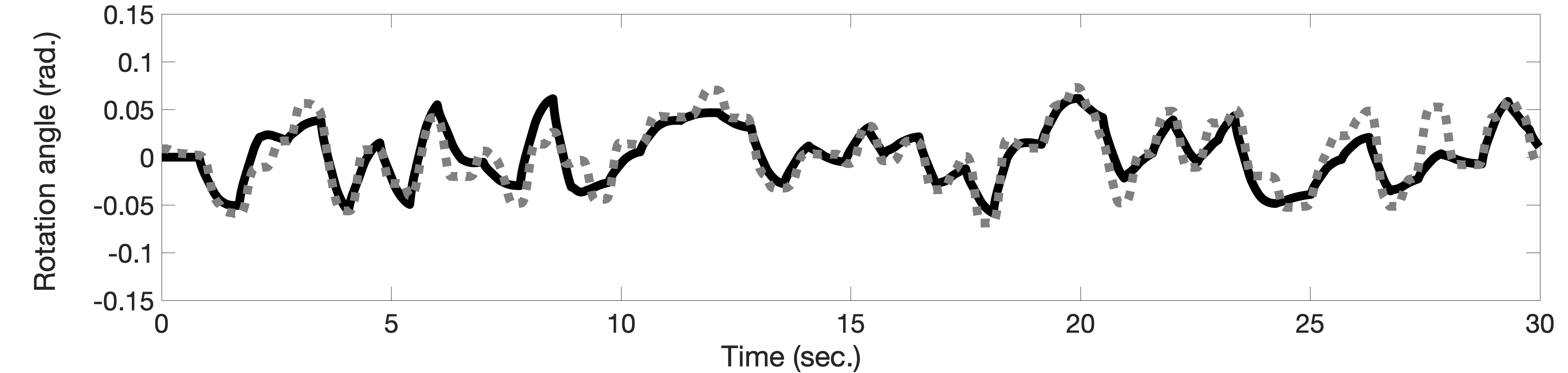
(j) Subject 10

Figure 4: The curve fitting with 10 experimental cases (continued). Solid lines represent estimated responses from the fitted models and dotted lines represent measured responses.

Subject	Improvement ($\%$)
1	69.25
2	65.79
3	74.83
4	89.36
5	87.44
6	65.02
7	53.62
8	77.70
9	63.44
10	67.62
Avg.	71.41

Table 2: Improvement on the variance of estimated parameters in an experiment study. The given values are $(1-\frac{{\sigma}^{2,\text{Lasso}}}{{\sigma}^{2,\text{All}}})\times 100$. ${\sigma}^{2,\text{Lasso}}$ is the variance of estimated parameters obtained from our method, and ${\sigma}^{2,\text{All}}$ is the variance of estimated parameters without regularization.

3.3 The Experiment

As shown in Fig. 2, each subject wears a helmet attached with two string potentiometers measuring the axial rotation of the head. Subjects rotated their heads about the vertical axis to track the command signals on the display. The command signal $r(t)$ is a pseudorandom sequence of steps with random step durations and amplitudes. The angle of the signal is bounded between $\pm 4^{\circ}$. The output signal $y(t)$ is the head rotation angle. Each subject performed three 30-second trials, and the sampling rate was 60 Hz ramadan2018selecting .

3.4 Simulation study

In this section, we analyze the bias and variance of estimated parameters from a simulation study with the known true parameters for comparison. First, we generate the simulated data $(\bm{x},\bm{y})$ where $\bm{x}\in\mathbb{R}^{1800\times 1}$ and $\bm{y}\in\mathbb{R}^{1800\times 1}$, which are the input and observation vectors, respectively. Additionally, we obtain 20 sets of nominal parameter values from preliminary estimation performed 20 times over all three trials for each subject. Finally, we evaluate our method by setting the mean of 20 sets of nominal parameter values as a set of typical values. In Fig. 3, as compared to the nonlinear least squares estimator without ${L}_{1}$-regularization, except for $\tau_{c}$, the biases of the other parameters were decreased by $28.0\%$ on average. In addition, the variances of all estimated parameters were decreased by $96.1\%$ on average.

3.5 In vivo experimental study

In this section, the variances of estimated parameters from our method are compared with the result of the standard simplex-based optimization in ramadan2018selecting . All parameters are pushed further toward the mean of nominal parameter values obtained from preliminary estimation as the regularization hyperparameter increases. The regularization hyperparameter increases until 5 sensitive parameters are selected. After selecting a sensitive parameter subset for each subject, we select the most frequent subset among all subjects for the fair comparison with ramadan2018selecting . The Lasso in ramadan2018selecting selected 5 parameters of $[{K}_{vcr}\ {K}_{ccr}\ \tau_{1A}\ \tau_{c}\ \tau_{CNS2}]$ as the most frequent subset of sensitive parameters, and the subset of $[{K}_{ccr}\ \tau\ \tau_{1A}\ \tau_{c}\ \tau_{CNS2}]$ was selected by our method. As a result, 4 out of 5 sensitive parameters $[{K}_{ccr}\ \tau_{1A}\ \tau_{c}\ \tau_{CNS2}]$ are selected by both methods.

Second, we evaluate our method based on the goodness of fit measured by variance accounted for (VAF). All values are given as mean $\pm$ standard deviation across subjects. The goodness of fit of our method ($\text{VAF}=82.5\%\pm 8.3\%$) over 10 subjects is almost equal to that of the Lasso ($\text{VAF}=83.3\%\pm 7.3\%$ ) in ramadan2018selecting . Without ${L}_{1}$-regularization, $\text{VAF}=84.9\%\pm 0.1\%$ over all subjects. In Fig. 4, for all subjects, the estimated responses are almost same as the measured responses, and the estimated responses are smoother than the measured responses.

Third, as shown in Table 2, the variance of estimated parameters is reduced by 71.4$\%$ on average across parameters and subjects as compared to those of estimated parameters without regularization.

Finally, we compute the average computation time using the “timeit” function from $MATLAB$ (The MathWorks Inc., Natick, MA, U.S.A.). The average computation time of our method for a subject is 54 times faster than that of the Lasso with the standard simplex-based optimization in ramadan2018selecting . In particular, the average computation time of our method across subjects is 5.6 seconds per trial, and that of the Lasso in ramadan2018selecting is 302.0 seconds per trial.

4 Discussion

We provided consistency and oracle properties (i.e., convergence to the correct sparsity and asymptotic normality) for a nonlinear regression approach with a generalized penalty function. As a result, we proved the existence of a local minimizer and the convergence to the sparse unknown parameters for the penalized nonlinear least squares estimator. It is important to note that for the first time, we have proved convergence properties of the penalized nonlinear least squares estimator, as compared to previous studies johnson2008penalized ; wu1981asymptotic ; fan2001scad .

In the simulation study, we showed that the bias and variance of estimated parameters of our method were decreased as compared to those of estimated parameters without ${L}_{1}$-regularization. When we set the mean of nominal parameter values as the typical values for non-selected estimates, the variance significantly was decreased. In addition, although the ${L}_{1}$-regularization is known to induce biased estimates, the bias with our method also slightly was decreased except for one parameter with the increased bias. The reason might be that our method pushes all parameters toward the mean of nominal parameter values obtained from 20 preliminary estimation. Therefore, if we set the appropriate values as the typical values, we could achieve lower values of bias and variance errors.

In the experimental study, our proposed method was compared with the Lasso in ramadan2018selecting using three performance criteria. First, we confirmed that the proposed method simultaneously selected and estimated sensitive parameters in the nonlinear model. As a result, five parameters were selected and estimated in our method, and the remaining parameters were fixed to the mean of nominal parameters obtained from preliminary estimation. With our method, 4 out of 5 sensitive parameters were the same as those selected in ramadan2018selecting . This result showed that our method behaved similarly in sensitive parameter selection by ramadan2018selecting using the Fisher information matrix. Selected sensitive parameters may vary slightly depending on the performance of the optimizer and the condition of initial points. However, they have not changed much over repeated randomized realizations. In addition, we presented VAF to quantitatively evaluate the goodness of fit of the estimated model. From the standard nonlinear least squares problem without ${L}_{1}$-regularization, VAF was about 84.9$\%$, and our method achieved about 82.5$\%$. Hence, the goodness of fit of the model estimated from our method was similar to that of model estimated from the standard nonlinear least squares problem without ${L}_{1}$-regularization although only 5 selected parameters were used for estimation in our method. Moreover, as shown in Fig. 4, most curve fitting errors occur around the peak points, which shows the limitation of the presented dynamics models that do not perfectly reflect the real physiological head-neck control processes. This could be due to the switching of human control strategies with sudden changes in head-neck orientations chen2002modeling .

Next, the model identifiability was improved by sensitive parameter selection from our method. The variance of estimated 12 parameters is reduced by $71.1\%$ on average. In general, when the number of parameters to be estimated is large with limited data, the model has poor (or lack of) identifiability. Therefore, through our method with key parameter selection, i.e., the nonlinear least squares problem with $L_{1}$-regularization on the deviation of parameters from the mean of the nominal parameter values, the uniqueness of the estimated solution can be ensured even for an original problem with a lack of identifiability due to limited data.

Finally, the average computation time of our method was 54 times faster than that of the Lasso with the brute force optimization algorithm in ramadan2018selecting . Our method reduced the computation time by eliminating large inverse matrix computation by modifying a Jacobian formulation as a minimization formulation.

5 Conclusions

In this paper, we tackled a parameter estimation problem with limited data by formulating it as a nonlinear least squares estimator with $L_{1}$-regularization.

We effectively improved the model identifiability by applying the Lasso to the nonlinear least squares problem. As asymptotic results, we provided consistency and oracle properties for a nonlinear regression approach with a generalized penalty function. Based on these results, we proposed a novel solution to our problem by solving the nonlinear least squares problem with ${L}_{1}$-regularization on the deviation of parameters from the nominal values in order to simultaneously select and estimate model parameters.

From simulation and experimental studies, we successfully demonstrated that the proposed method simultaneously selected and estimated sensitive parameters, improved the model identifiability by reducing the variance of estimated parameters and took a much shorter computation time than that of the Lasso in ramadan2018selecting .

Future work would be to apply our method to other clinical patient-specific calibration of the disease models do2018prediction ; zhang2019patient .

Conflict of interest

The authors declare that they have no conflict of interest.

Appendix A Proof of Lemma 1

We first find the lower bound of $\bm{Q}_{n}(\bm{\theta}_{0}+n^{-1/2}\bm{v})-\bm{Q}_{n}(\bm{\theta}_{0})$.

$$\bm{Q}_{n}(\bm{\theta}_{0}+n^{-1/2}\bm{v})-\bm{Q}_{n}(\bm{\theta}_{0})$$

$$=\bm{S}_{n}(\bm{\theta}_{0}+n^{-1/2}\bm{v})-\bm{S}_{n}(\bm{\theta}_{0})$$

$$~{}~{}~{}+n(\sum^{p}_{k=1}p_{\lambda_{n}}(|\theta_{0k}+n^{-1/2}v_{k}|)-\sum^{p}_{k=1}p_{\lambda_{n}}(|\theta_{0k}|))$$

$$=n^{-1/2}\left(\nabla\bm{S}_{n}(\bm{\theta}_{0})\right)^{T}\bm{v}+\frac{1}{2}n^{-1}\bm{v}^{T}\nabla^{2}\bm{S}_{n}(\bm{\theta}^{*})\bm{v}$$

$$~{}~{}~{}+n\left(\sum^{s}_{k=1}p_{\lambda_{n}}(|\theta_{0k}+n^{-1/2}v_{k}|)-\sum^{s}_{k=1}p_{\lambda_{n}}(|\theta_{0k}|)\right)$$

$$~{}~{}~{}+n\sum^{p}_{k=s+1}p_{\lambda_{n}}(|\theta_{0k}+n^{-1/2}v_{k}|),\text{where}$$

$$~{}~{}~{}\hbox{$\bm{\theta}^{*}=(\theta^{*}_{1},\theta^{*}_{2},\ldots,\theta^{*}_{p})$ lies between $\bm{\theta}_{0}+n^{-1/2}\bm{v}$ and $\bm{\theta}_{0}$},$$

$$=n^{-1/2}\left(\nabla\bm{S}_{n}(\bm{\theta}_{0})\right)^{T}\bm{v}+\frac{1}{2}n^{-1}v^{T}\nabla^{2}\bm{S}_{n}(\bm{\theta}^{*})v$$

$$~{}~{}+n\left(\sum^{s}_{k=1}q_{\lambda_{n}}(|\theta^{*}_{0k}|)\text{sgn}(\theta^{*}_{0k})n^{-1/2}v_{k}\right)$$

$$~{}~{}+n\sum^{p}_{k=s+1}p_{\lambda_{n}}(|\theta_{k}+n^{-1/2}v|)$$

$$\geq n^{-1/2}(\nabla\bm{S}_{n}(\bm{\theta}_{0}))^{T}\bm{v}+\frac{1}{2}n^{-1}v^{T}\nabla^{2}\bm{S}_{n}(\bm{\theta}^{*})(v)$$

$$~{}~{}+n\left(\sum^{s}_{k=1}q_{\lambda_{n}}(|\theta^{*}_{0k}|)\text{sgn}(\theta^{*}_{0k})n^{-1/2}v_{k}\right)$$

$$:=\mathbb{A}+\mathbb{B}+\mathbb{C}.$$

For the sake of simplicity,
we define ${\bm{d}}=(d_{1}(\bm{\theta},\bm{\theta}^{\prime}),...,d_{n}(\bm{\theta},\bm{\theta}^{\prime}))$, where $d_{i}(\bm{\theta},\bm{\theta}^{\prime})=f({\bm{x}}_{i};\bm{\theta})-f({\bm{x}}_{i};\bm{\theta}^{\prime})$. For the term $\mathbb{A}$,

$$n^{-1/2}(\nabla\bm{S}_{n}(\bm{\theta}_{0}))^{T}\bm{v}$$

$$~{}~{}~{}=-2n^{-1/2}\bm{v}^{T}\bm{\dot{F}}(\bm{\theta}_{0})\bm{\epsilon},$$

$$~{}~{}~{}=-2\bm{v}^{T}\left[\bm{F}_{n}^{1/2}\left(\bm{\dot{F}(\theta_{0})}^{T}\bm{\dot{F}(\theta_{0})}\right)^{-1/2}\bm{\bm{\dot{F}}}(\bm{\theta}_{0})^{T}\bm{\epsilon}\right],$$

$$~{}~{}~{}\hbox{where }\bm{F}_{0}=\frac{1}{n}\bm{\dot{F}(\theta_{0})}^{T}\bm{\dot{F}(\theta_{0})}.$$

By Assumption 1, $\bm{F}_{0}^{1/2}\ \rightarrow\ \Gamma^{1/2}$ and we claim that,

$$\left(\bm{\dot{F}}(\bm{\theta}_{0})^{T}{\bm{\dot{F}}}(\bm{\theta}_{0})\right)^{-1/2}{\bm{\dot{F}}}(\bm{\theta}_{0})^{T}{\bm{\epsilon}}~{}\stackrel{{\scriptstyle d}}{{\longrightarrow}}N(0,\sigma^{2}I).$$

The claim follows from the lemma 2.1 in huber1973robust . The condition for the lemma in our setting is

$$\left\|\bm{\dot{F}}(\bm{\theta}_{0})\left(\bm{\dot{F}}(\bm{\theta}_{0})^{T}{\bm{\dot{F}}}(\bm{\theta}_{0})\right)^{-1/2}\right\|_{\infty}\rightarrow 0$$

where $\|A\|_{\infty}$ denote the maximum absolute value of all elements of matrix $A$. Since $\bm{\dot{F}}(\bm{\theta}_{0})$ is an $n\times p$ matrix and $\left(\bm{\dot{F}}(\bm{\theta}_{0})^{T}{\bm{\dot{F}}}(\bm{\theta}_{0})\right)^{-1/2}$ is a $p\times p$ matrix,

$$\left\|\bm{\dot{F}}(\bm{\theta}_{0})\left(\bm{\dot{F}}(\bm{\theta}_{0})^{T}{\bm{\dot{F}}}(\bm{\theta}_{0})\right)^{-1/2}\right\|_{\infty}$$

$$\leq p\left\|\left(\bm{\dot{F}}(\bm{\theta}_{0})^{T}{\bm{\dot{F}}}(\bm{\theta}_{0})\right)^{-1/2}\right\|_{\infty}\left\|\bm{\dot{F}}(\bm{\theta}_{0})\right\|_{\infty}$$

$$=pn^{-1/2}\left\|\bm{F}_{0}^{-1/2}\right\|_{\infty}\left\|\bm{\dot{F}}(\bm{\theta}_{0})\right\|_{\infty}$$

$$=O\left(\frac{p}{\sqrt{n}}\right).$$

The first and second conditions from Assumption 1 imply the last equality. Therefore, we have

$$-2\bm{v}^{T}\left[\bm{F}_{0}^{1/2}\left(\bm{\dot{F}(\theta_{0})}^{T}\bm{\dot{F}(\theta_{0})}\right)^{-1/2}\bm{\bm{\dot{F}}}(\bm{\theta}_{0})^{T}\bm{\epsilon}\right]$$ (1)

$$~{}\stackrel{{\scriptstyle d}}{{\longrightarrow}}~{}N(0,4\sigma^{2}\bm{v}^{T}\Gamma\bm{v}).$$

For the term $\mathbb{B}$,

$$\frac{1}{2}n^{-1}\bm{v}^{T}\nabla^{2}\bm{S}_{n}(\bm{\theta}^{*})\bm{v}$$

$$=n^{-1}\bm{v}^{T}\left\{\left({\bm{\dot{F}}}(\bm{\theta}^{*})^{T}{\bm{\dot{F}}}(\bm{\theta}^{*})\right)+{\bm{{\ddot{F}}}}(\bm{\theta}^{*})^{T}(I\otimes(\bm{d}-\bm{\epsilon}))\right\}\bm{v}$$

$$=\bm{v}^{T}\left[\frac{\left({\bm{\dot{F}}}(\bm{\theta_{0}})^{T}{\bm{\dot{F}}}(\bm{\theta_{0}})\right)}{n}\bm{Z}^{-1}_{n}\bm{v}\right],\hbox{where}$$

$$~{}~{}~{}\bm{Z}_{n}=\left\{\left({\bm{\dot{F}}}(\bm{\theta}^{*})^{T}{\bm{\dot{F}}}(\bm{\theta}^{*})\right)+{\bm{{\ddot{F}}}}(\bm{\theta}^{*})^{T}(I\otimes(\bm{d}-\bm{\epsilon})\right\}^{-1}n\bm{F}_{0}.$$

If we show $\bm{Z_{n}}^{-1}\stackrel{{\scriptstyle p}}{{\rightarrow}}I$, with Assumption 1, we obtain

$$\mathbb{A}+\mathbb{B}~{}\stackrel{{\scriptstyle d}}{{\longrightarrow}}~{}N(\bm{v}^{T}\Gamma\bm{v},4\sigma^{2}\bm{v}^{T}\Gamma\bm{v}).$$ (2)

$\bm{Z_{n}}^{-1}$ can be rewritten as,

$$\bm{Z_{n}^{-1}} =\left(n\bm{F}_{0}\right)^{-1}\left\{\left({\bm{\dot{F}}}(\bm{\theta}^{*})^{T}{\bm{\dot{F}}}(\bm{\theta}^{*})\right)+\bm{{\ddot{F}}}(\bm{\theta}^{*})^{T}(I\otimes(\bm{d}-\bm{\epsilon})\right\}$$

$$=\left(n\bm{F}_{0}\right)^{-1}\left({\bm{\dot{F}}}(\bm{\theta}^{*})^{T}{\bm{\dot{F}}}(\bm{\theta}^{*})\right)+\left(n\bm{F}_{0}\right)^{-1}\bm{{\ddot{F}}}(\bm{\theta}^{*})^{T}(I\otimes\bm{d})$$

$$-\left(n\bm{F}_{0}\right)^{-1}\bm{{\ddot{F}}}(\bm{\theta}^{*})^{T}(I\otimes\bm{\epsilon}).$$

By Assumption 1, the first term converges to $I$ almost surely. By the conditions 1, 2, and 4 of Assumption 1 and Cauchy-Schwarz inequality, the second term converges to zero almost surely. For the last term, it is enough to show that

$$\frac{1}{n}\bm{f_{ks}}(\bm{\theta})^{T}\bm{\epsilon}\ \stackrel{{\scriptstyle p}}{{\longrightarrow}}0$$ (3)

uniformly on $S-\{\theta\in\Theta:\|\theta-\theta_{0}\|\leq\delta\}$ with probability 1, because of the conditions 1 and 2 of Assumption 1. Then, by the condition 4 of Assumption 1, (3.17) can be shown in a manner similar to that of wu1981asymptotic For the term $\mathbb{C}$, by Assumption 2 for a fixed $s<\infty$,

$$\left(n^{1/2}\sum^{s}_{k=1}q_{\lambda_{n}}(|\theta^{*}_{0k}|)\text{sgn}(\theta^{*}_{0k})v_{k}\right)~{}\longrightarrow~{}0.$$ (4)

Thus, combined (2) with (4), we have

$$\mathbb{A}+\mathbb{B}+\mathbb{C}~{}\stackrel{{\scriptstyle d}}{{\longrightarrow}}~{}N(\bm{v}^{T}\Gamma\bm{v},4\sigma^{2}\bm{v}^{T}\Gamma\bm{v}),$$

which leads to the desired result for large enough $C$.

Appendix B Proof of Theorem 1

By Lemma 1 and the continuity of $\bm{Q}_{n}(\cdot)$, we obtain Theorem 1.

Appendix C Proof of Theorem 2

Proof of (i)
First, we break $M_{k}$ into two sets:

$$M_{k} =\left\{\omega:\hat{\theta}_{k}\neq 0,|\hat{\theta}_{k}|\geq Cn^{-1/2}\right\}$$

$$~{}~{}~{}~{}+\left\{\omega:\hat{\theta}_{k}\neq 0,|\hat{\theta}_{k}|<Cn^{-1/2}\right\}$$

$$=:E_{n}+F_{n}.$$

Then, it is enough to show for any $\epsilon>0$, $P(E_{n})<\epsilon/2$ and $P(F_{n})<\epsilon/2$. For any $\epsilon>0$, we can show $P(E_{n})<\epsilon/2$ for large enough $n$ because of the consistency.

To verify $P(F_{n})<\epsilon/2$ for large enough $n$, we first show $n^{1/2}q_{\lambda_{n}}(|\hat{\theta}_{k}|)=O_{p}(1)$ on the set $F_{n}$. Note that

$$n^{-1/2}\nabla\bm{S}_{n}(\bm{\theta})-n^{-1/2}\nabla\bm{S}_{n}(\bm{\theta}_{0})$$

$$=n^{-1/2}\nabla^{2}\bm{S}_{n}(\bm{\theta}^{**})(\bm{\theta}-\bm{\theta}_{0})$$

$$=n^{1/2}\frac{\left({\bm{\dot{F}}}(\bm{\theta}^{**})^{T}{\bm{\bm{\dot{}}{F}}}(\bm{\theta}^{**})\right)}{n}\bm{Z}^{-1}_{n}(\bm{\theta}-\bm{\theta}_{0})=O_{p}(1),$$

where $\bm{\theta}^{**}$ lies between $\bm{\theta}$ and $\bm{\theta}_{0}$. Since $\frac{1}{n}{\bm{\dot{F}}}(\bm{\theta}^{**})^{T}{\bm{\dot{F}}}(\bm{\theta}^{**})~{}\stackrel{{\scriptstyle p}}{{\longrightarrow}}~{}\Gamma$, $\bm{Z}^{-1}_{n}~{}\stackrel{{\scriptstyle p}}{{\longrightarrow}}~{}I$ and $\|\bm{\theta}-\bm{\theta}_{0}\|=O_{p}(n^{-1/2}).$ Thus, we have

$$\sup_{\|\theta-\theta_{0}\|\leq Cn^{-1/2}}\|n^{-1/2}\nabla\bm{S}_{n}(\bm{\theta})-n^{-1/2}\nabla\bm{S}_{n}(\bm{\theta}_{0})\|=O_{p}(1).$$ (1)

Combining (1) with $\|n^{-1/2}\nabla S_{n}(\theta_{0})\|=O_{p}(1)$, we have

$$\|n^{-1/2}\nabla\bm{S}_{n}(\bm{\theta})\|=O_{p}(1)$$ (2)

for $\bm{\theta}$ which satisfies $\|\bm{\theta}-\bm{\theta}_{0}\|\leq Cn^{-1/2}.$ Since $\hat{\bm{\theta}}$ is the local minimizer of $\bm{Q}_{n}(\bm{\theta})$ with the root-n-consistent, we attain

$${}n^{1/2}q_{\lambda_{n}}(|\hat{\theta}_{k}|)=O_{p}(1)$$ (3)

from

$$n^{-1/2}\frac{\partial\bm{Q}_{n}(\bm{\theta})}{\partial\theta_{k}}\Big{|}_{\bm{\theta}=\hat{\bm{\theta}}}$$

$$~{}~{}~{}~{}~{}~{}~{}~{}~{}~{}~{}~{}~{}~{}~{}=n^{-1/2}\frac{\partial\bm{S}_{n}(\bm{\theta})}{\partial\theta_{k}}\Big{|}_{\bm{\theta}=\hat{\bm{\theta}}}+n^{1/2}q_{\lambda_{n}}(|\hat{\theta_{k}}|)\text{sgn}(\hat{\theta}_{k}).$$

Therefore, there exists $M^{\prime}$ such that, for large enough $n$,

$$P\{\omega:\hat{\theta}_{k}\neq 0,|\hat{\theta}_{k}|<Cn^{-1/2},n^{1/2}q_{\lambda_{n}}(|\hat{\theta}_{k}|)>M^{\prime}\}<\epsilon/2.$$

In addition, by the second assumption of Assumption 2,

$$\{\omega:\hat{\theta}_{k}\neq 0,|\hat{\theta}_{k}|<Cn^{-1/2},n^{1/2}q_{\lambda_{n}}(|\hat{\theta}_{k}|)>M^{\prime}\}$$

$$~{}~{}~{}~{}~{}~{}~{}~{}~{}~{}~{}~{}~{}~{}~{}~{}~{}~{}~{}~{}~{}~{}~{}~{}=\{\omega:\hat{\theta}_{k}\neq 0,|\hat{\theta}_{k}|<Cn^{-1/2}\}$$

for the large enough $n$, which leads to $P(F_{n})<\epsilon/2$ for large enough $n$.

Proof of (ii)
By the Taylor expansion,

$$n^{-1/2}\nabla\bm{Q}_{n}(\hat{\bm{\theta}}) = n^{-1/2}\nabla\bm{S}_{n}(\hat{\bm{\theta}})+n^{-1/2}{\bm{q}}_{\lambda_{n}}(\hat{\bm{\theta}})\cdot\text{sgn}(\hat{\bm{\theta}})$$

$$= n^{-1/2}\left(\nabla\bm{S}_{n}(\bm{\theta}_{0})+\nabla^{2}\bm{S}_{n}(\bm{\theta}^{**})(\hat{\bm{\theta}}-\bm{\theta}_{0})\right)$$

$$~{}+n^{1/2}{\bm{q}}_{\lambda_{n}}(\hat{\bm{\theta}})\cdot\text{sgn}(\hat{\bm{\theta}})$$

where ${\bm{q}}_{\lambda_{n}}(\hat{\bm{\theta}})\cdot\text{sgn}(\hat{\bm{\theta}})=\left(q_{\lambda_{n}}(|\hat{\theta}_{1}|)\text{sgn}(\hat{\theta}_{1}),..,q_{\lambda_{n}}(|\hat{\theta}_{p}|)\times\right.$ $\left.\text{sgn}(\hat{\theta}_{p})\right)^{T}.$ Since $\hat{\bm{\theta}}$ is the local minimizer of $\bm{Q}_{n}({\bm{\theta}})$, $\nabla\bm{Q}_{n}(\hat{\bm{\theta}})=0$ so that

$$n^{-1/2}(-\nabla\bm{S}_{n}({\bm{\theta}_{0}}))= n^{-1}\nabla^{2}S_{n}(\bm{\theta}^{**})\left(n^{1/2}(\hat{\bm{\theta}}-\bm{\theta}_{0})\right)$$

$$+n^{1/2}{\bm{q}}_{\lambda_{n}}(\hat{\bm{\theta}})\cdot\text{sgn}(\hat{\bm{\theta}}).$$

Finally,

$$n^{1/2}2\Gamma_{11}({\hat{\bf{\bm{\theta}}}}_{11}-\bm{\theta}_{01}+(2\Gamma_{11})^{-1}b_{n})~{}\stackrel{{\scriptstyle d}}{{\longrightarrow}}~{}N(0,4\Gamma_{11}\sigma^{2}),$$

because $n^{-1}\nabla^{2}\bm{S}_{n}(\bm{\theta}^{**})\stackrel{{\scriptstyle p}}{{\longrightarrow}}2\Gamma$, $n^{-1/2}(-\nabla\bm{S}_{n}({\bm{\theta}_{0}}))\stackrel{{\scriptstyle d}}{{\longrightarrow}}$ $N({\bm{0}},4\Gamma\sigma^{2})$ and the consistency of $\hat{\bm{\theta}}$.

Appendix D Nonlinear least squares estimator with ${L}_{1}$-regularization.

In order to apply the Lasso to the nonlinear least squares problem, we reformulate the Levenberg-Marquardt (LM) optimization algorithm as a linear least squares problem as follow.

$${\hat{\tilde{\bm{\theta}}}}^{j+1} =\min\limits_{{\tilde{\bm{\theta}}}}\|\bm{\Lambda}{\tilde{\bm{\theta}}}^{j+1}-\bm{\Lambda}{\tilde{\bm{\theta}}}^{j}+\bm{J}^{T}{\tilde{\bm{r}}}({\tilde{\bm{\theta}}}^{j})\|^{2}_{2}$$ (1)

$$\quad\ s.t.\ \sum^{p}_{k=1}|\tilde{\theta}^{j+1}_{k}|\leq{T}_{\theta},$$

where ${\tilde{\bm{\theta}}}^{j+1}={\tilde{\bm{\theta}}}^{j}+\Delta\bm{\theta},\Delta\bm{\theta}=-\bm{\Lambda}^{-1}\bm{J}^{T}{\tilde{\bm{r}}}({\tilde{\bm{\theta}}}^{j}),\bm{\Lambda}=(\bm{J}^{T}\bm{J}+\mu\text{diag}(\bm{J}^{T}\bm{J}))$. The residual vector ${\tilde{\bm{r}}}({\tilde{\bm{\theta}}}^{j})=\bm{r}({\tilde{\bm{\theta}}}^{j}+{\bar{\bm{\theta}}})=\bm{r}(\bm{\theta}^{j})=\bm{y}-{f}(\bm{X};\bm{\theta}^{j})$. ${T}_{\theta}$ is the regularization hyperparameter. The sum of the deviation of parameters from the mean of the nominal parameter values is less than or equal to the regularization hyperparameter ${T}_{\theta}$. The damping factor $\mu$ affects the efficiency and the convergence stability cui2017new . $\bm{J}$ is the Jacobian matrix which consists of all first-order partial derivatives of the residual vector with respect to the parameters, evaluated for ${\tilde{\bm{\theta}}}={\tilde{\bm{\theta}}}^{j}$ as follows.

$$\bm{J}:=\frac{\partial{\tilde{\bm{r}}}({\tilde{\bm{\theta}}}^{j})}{\partial{\tilde{\bm{\theta}}}^{j}}$$

In addition, as compared with the conventional Lasso fixing insensitive parameters to 0, our method simultaneously selects and estimates only sensitive parameters while fixing insensitive parameters onto the mean of the nominal parameter values ${\bar{\bm{\theta}}}$.

Table 3: The algorithm of sensitive parameter selection using our method

Input:	(1) Experimental Data and Dynamical Model (2) Vector of Normalized Values (${\bar{\bm{\Phi}}}$), where the Mean of Nominal Parameter Values is ${\bar{\bm{\theta}}}$ (3) Desired Optimal Number of Sensitive Parameters (${{n}^{*}}$) (4) The Regularization Hyperparameter ${T}_{\theta}$
Output:	(1) A Subset of the Sensitive Parameters ($\hat{\tilde{\bm{\theta}}}$)
1:$\text{NumParams}=0$ 2:${T}_{\theta}=1.0$ 3:while $\text{NumParams}\hskip 5.0pt!={{n}^{*}}$ do 4:   repeat 5:      Solve (1) in Appendix D 6:   until $\tilde{\bm{\Phi}}$ convergences 7:   for $i=1:n$ do 8:      if $\hat{\tilde{\bm{\Phi}}}(i)>0.001$ then 9:         NumParams = NumParams + 1 10:      end if 11:   end for 12:   if $\text{NumParams}\hskip 5.0pt!={{n}^{*}}$ then 13:      ${T}_{\theta}={T}_{\theta}-\frac{\text{NumParams}-{{n}^{*}}}{i+{n}^{*}}$ 14:   end if 15:end while 16:${\hat{\tilde{\bm{\theta}}}}$, where a subset of the normalized sensitive parameters is $\hat{\tilde{\bm{\Phi}}}$

References

- (1) Babyak, M.A.: What you see may not be what you get: a brief, nontechnical introduction to overfitting in regression-type models. Psychosomatic medicine 66(3), 411–421 (2004)
- (2) Chen, K.J., Keshner, E., Peterson, B., Hain, T.: Modeling head tracking of visual targets. Journal of Vestibular Research 12(1), 25–33 (2002)
- (3) Cui, M., Zhao, Y., Xu, B., Gao, X.w.: A new approach for determining damping factors in levenberg-marquardt algorithm for solving an inverse heat conduction problem. International Journal of Heat and Mass Transfer 107, 747–754 (2017)
- (4) Do, H.N., Choi, J., Lim, C.Y., Maiti, T.: Appearance-based localization of mobile robots using group lasso regression. Journal of Dynamic Systems, Measurement, and Control 140(9), 091016 (2018)
- (5) Do, H.N., Ijaz, A., Gharahi, H., Zambrano, B., Choi, J., Lee, W., Baek, S.: Prediction of abdominal aortic aneurysm growth using dynamical gaussian process implicit surface. IEEE Transactions on Biomedical Engineering (2018)
- (6) Fan, J., Li, R.: Variable selection via nonconcave penlized likelihood and its oracla properties. Journal of the American Statistical Association 96(456), 1348–1360 (2001)
- (7) Gutenkunst, R.N., Waterfall, J.J., Casey, F.P., Brown, K.S., Myers, C.R., Sethna, J.P.: Universally sloppy parameter sensitivities in systems biology models. PLoS computational biology 3(10), e189 (2007)
- (8) Huber, P.J., et al.: Robust regression: asymptotics, conjectures and monte carlo. The Annals of Statistics 1(5), 799–821 (1973)
- (9) Johnson, B.A., Lin, D., Zeng, D.: Penalized estimating functions and variable selection in semiparametric regression models. Journal of the American Statistical Association 103(482), 672–680 (2008)
- (10) Jolliffe, I.T., Trendafilov, N.T., Uddin, M.: A modified principal component technique based on the lasso. Journal of computational and Graphical Statistics 12(3), 531–547 (2003)
- (11) Kump, P., Bai, E.W., Chan, K.S., Eichinger, B., Li, K.: Variable selection via rival (removing irrelevant variables amidst lasso iterations) and its application to nuclear material detection. Automatica 48(9), 2107–2115 (2012)
- (12) Kyubaek, Y., Jongeun, C.: Penalized nonlinear regression with application to head-neck position tracking. In: ASME 2019 Dynamic Systems and Control Conference. American Society of Mechanical Engineers Digital Collection (in press)
- (13) Little, M.P., Heidenreich, W.F., Li, G.: Parameter identifiability and redundancy: theoretical considerations. PloS one 5(1), e8915 (2010)
- (14) Lund, A., Dyke, S.J., Song, W., Bilionis, I.: Global sensitivity analysis for the design of nonlinear identification experiments. Nonlinear Dynamics 98(1), 375–394 (2019)
- (15) Moré, J.J.: The levenberg-marquardt algorithm: implementation and theory. In: Numerical analysis, pp. 105–116. Springer (1978)
- (16) Peng, G., Hain, T., Peterson, B.: A dynamical model for reflex activated head movements in the horizontal plane. Biological cybernetics 75(4), 309–319 (1996)
- (17) Pitt, M.A., Myung, I.J.: When a good fit can be bad. Trends in cognitive sciences 6(10), 421–425 (2002)
- (18) Popovich Jr, J.M., Reeves, N.P., Priess, M.C., Cholewicki, J., Choi, J., Radcliffe, C.J.: Quantitative measures of sagittal plane head–neck control: A test–retest reliability study. Journal of biomechanics 48(3), 549–554 (2015)
- (19) Qin, P., Nishii, R., Yang, Z.J.: Selection of narx models estimated using weighted least squares method via gic-based method and l 1-norm regularization methods. Nonlinear Dynamics 70(3), 1831–1846 (2012)
- (20) Ramadan, A., Boss, C., Choi, J., Reeves, N.P., Cholewicki, J., Popovich, J.M., Radcliffe, C.J.: Selecting sensitive parameter subsets in dynamical models with application to biomechanical system identification. Journal of biomechanical engineering 140(7), 074503 (2018)
- (21) Ramadan, A., Choi, J., Cholewicki, J., Reeves, N.P., Popovich, J.M., Radcliffe, C.J.: Feasibility of incorporating test-retest reliability and model diversity in identification of key neuromuscular pathways during head position tracking. IEEE transactions on neural systems and rehabilitation engineering (2019)
- (22) Rasouli, M., Westwick, D., Rosehart, W.: Reducing induction motor identified parameters using a nonlinear lasso method. Electric Power Systems Research 88, 1–8 (2012)
- (23) Tibshirani, R.: Regression shrinkage and selection via the lasso. Journal of the Royal Statistical Society. Series B (Methodological) pp. 267–288 (1996)
- (24) Tibshirani, R., Saunders, M., Rosset, S., Zhu, J., Knight, K.: Sparsity and smoothness via the fused lasso. Journal of the Royal Statistical Society: Series B (Statistical Methodology) 67(1), 91–108 (2005)
- (25) Tibshirani, R., Wasserman, L.A.: Sensitive parameters. Canadian Journal of Statistics 16(2), 185–192 (1988)
- (26) Wu, C.F.: Asymptotic theory of nonlinear least squares estimation. The Annals of Statistics pp. 501–513 (1981)
- (27) Yuan, M., Lin, Y.: Model selection and estimation in regression with grouped variables. Journal of the Royal Statistical Society: Series B (Statistical Methodology) 68(1), 49–67 (2006)
- (28) Zhang, L., Jiang, Z., Choi, J., Lim, C.Y., Maiti, T., Baek, S.: Patient-specific prediction of abdominal aortic aneurysm expansion using bayesian calibration. IEEE Journal of Biomedical and Health Informatics (2019)
- (29) Zou, H.: The adaptive lasso and its oracle properties. Journal of the American statistical association 101(476), 1418–1429 (2006)
- (30) Zou, H., Hastie, T.: Regularization and variable selection via the elastic net. Journal of the Royal Statistical Society: Series B (Statistical Methodology) 67(2), 301–320 (2005)