Reduced order models for Lagrangian Hydrodynamics

Abstract

As a mathematical model of high-speed flow and shock wave propagation in a complex multimaterial setting, Lagrangian hydrodynamics is characterized by moving meshes, advection-dominated solutions, and moving shock fronts with sharp gradients. These challenges hinder the existing projection-based model reduction schemes from being practical. We develop several variations of projection-based reduced order model techniques for Lagrangian hydrodynamics by introducing three different reduced bases for position, velocity, and energy fields. A time-windowing approach is also developed to address the challenge imposed by the advection-dominated solutions. Lagrangian hydrodynamics is formulated as a nonlinear problem, which requires a proper hyper-reduction technique. Therefore, we apply the over-sampling DEIM and SNS approaches to reduce the complexity due to the nonlinear terms. Finally, we also present both a posteriori and a priori error bounds associated with our reduced order model. We compare the performance of the spatial and time-windowing reduced order modeling approaches in terms of accuracy and speed-up with respect to the corresponding full order model for several numerical examples, namely Sedov blast, Gresho vortices, Taylor-Green vortices, and triple-point problems.

1 Introduction

Physical simulations are key to developments in science, engineering, and technology. Many physical processes are mathematically modeled by time-dependent nonlinear partial differential equations. In many applications, the analytical solution of such problems can not be obtained, and numerical methods are developed to approximate the solutions efficiently. However, subject to the complexity of the model problem and the size of the problem domain, the computational cost can be prohibitively high. It may take a long time to run one forward simulation even with high performance computing. In decision-making applications where multiple forward simulations are needed, such as parameter study, design optimization [1, 2, 3, 4], optimal control [5, 6], uncertainty quantification [7, 8], and inverse problems [9, 8], the computationally expensive simulations are not desirable. To this end, a reduced order model (ROM) can be useful in this context to obtain sufficiently accurate approximate solutions with considerable speed-up compared to a corresponding full order model (FOM).

Many model reduction schemes have been developed to reduce the computational cost of simulations while minimizing the error introduced in the reduction process. Most of these approaches seek to extract an intrinsic solution subspace for condensed solution representation by a linear combination of reduced basis vectors. The reduced basis vectors are extracted from performing proper orthogonal decomposition (POD) on the snapshot data of the FOM simulations. The number of degrees of freedom is then reduced by substituting the ROM solution representation into the (semi-)discretized governing equation. These approaches take advantage of both the known governing equation and the solution data generated from the corresponding FOM simulations to form linear subspace reduced order models (LS-ROM). Example applications include, but are not limited to, the nonlinear diffusion equations [10, 11], the Burgers equation and the Euler equations in small-scale [12, 13, 14], the convection–diffusion equations [15, 16], the Navier–Stokes equations [17, 18], rocket nozzle shape design [19], flutter avoidance wing shape optimization [20], topology optimization of wind turbine blades [21], lattice structure design [22], porous media flow/reservoir simulations [23, 24, 25, 26], computational electro-cardiology [27], inverse problems [28], shallow water equations [29, 30], Boltzmann transport problems [31], computing electromyography [32], spatio-temporal dynamics of a predator–prey system [33], acoustic wave-driven microfluidic biochips [34], and Schrödinger equation [35]. Survey papers for the projection-based LS-ROM techniques can be found in [36, 37].

In spite of successes of the classical LS-ROM in many applications, these approaches are limited to the assumption that the intrinsic solution space falls into a subspace with a small dimension, i.e., the solution space has a small Kolmogorov $n$-width. This assumption is violated in advection-dominated problems, such as sharp gradients, moving shock fronts, and turbulence, which hinders these model reduction schemes from being practical. Our goal in this paper is to develop an efficient reduced order model for hydrodynamics simulation. Some reduced order model techniques for hydrodynamics or turbulence models in the literature include [38, 39, 40, 41, 42, 43, 44], which are mostly built on the Eulerian formulation, i.e., the computational mesh is stationary with respect to the fluid motion. In contrast, numerical methods in the Lagrangian formulation, which are characterized by a computational mesh that moves along with the fluid velocity, are developed for better capturing the shocks and preserving the conserved quantities in advection-dominated problems. It therefore becomes natural to develop Lagrangian-based reduced order models to overcome the challenges posed by advection-dominated problems. Some existing work in this research direction include [15, 45], where a Lagrangian POD and dynamic mode decomposition (DMD) reduced order model are introduced respectively for the one-dimensional nonlinear advection-diffusion equation. We remark that there are some similarities and differences between our work and [15] in using POD for developing Lagrangian-based reduced order models. It is important to note that our work is based on the more complicated and challenging two-dimensional or three-dimensional compressible Euler equations. Additionally, the reduced bases are built independently for each state variable in our work, while a single basis is built for the whole state in [15]. Furthermore, we introduce the time-windowing concept so as to ensure adequate ROM speed-up by decomposing the time frame into small time windows and building a temporally-local ROM for each window.

Recently, there have been many attempts to develop efficient ROMs for the advection-dominated or sharp gradient problems. The attempts can be divided mainly into two categories. The first category enhances the solution representability of the linear subspace by introducing some special treatments and adaptive schemes. A dictionary-based model reduction method for the approximation of nonlinear hyperbolic equations is developed in [46], where the reduced approximation is obtained from the minimization of the residual in the $L_{1}$ norm for the reduced linear subspace. In [47], a fail-safe $h$-adaptive algorithm is developed. The algorithm enables ROMs to be incrementally refined to capture the shock phenomena which are unobserved in the original reduced basis through a-posteriori online enrichment of the reduced-basis space by decomposing a given basis vector into several vectors with disjoint support. The windowed least-squares Petrov–Galerkin model reduction for dynamical systems with implicit time integrators is introduced in [48, 49], which can overcome the challenges arising from the advection-dominated problems by representing only a small time window with a local ROM. Another active research direction is to exploit the sharp gradients and represent spatially local features in ROM, such as the online adaptivity bases and adaptive sampling approach [50] and the shock reconstruction surrogate approach [51]. In [52], an adaptive space-time registration-based model reduction is used to align local features of parameterized hyperbolic PDEs in a fixed one-dimensional reference domain. Some new approaches have been developed for aligning the sharp gradients by using a superposition of snapshots with shifts or transforms. In [53], the shifted proper orthogonal decomposition (sPOD) introduces time-dependent shifts of the snapshot matrix in POD in an attempt to separate different transport velocities in advection-dominated problems. The practicality of this approach relies heavily on accurate determination of shifted velocities. In [54], an iterative transport reversal algorithm is proposed to decompose the snapshot matrix into multiple shifting profiles. In [55], inspired by the template fitting [56], a high resolution transformed snapshot interpolation with an appropriate behavior near singularities is considered.

The second category replaces the linear subspace solution representation with the nonlinear manifold, which is a very active research direction. Recently, a neural network-based reduced order model is developed in [57] and extended to preserve the conserved quantities in the physical conservation laws [58]. In these approaches, the weights and biases in the neural network are determined in the training phase, and existing numerical methods, such as finite difference and finite element methods, are utilized. However, since the nonlinear terms need to be updated every time step or Newton step, and the computation of the nonlinear terms still scale with the FOM size, these approaches do not achieve any speed-up with respect to the corresponding FOM. Recently, Kim, et al., have achieved a considerable speed-up with the nonlinear manifold reduced order model [59, 60], but it was only applied to small problems. Manifold approximations via transported subspaces in [61] introduced a low-rank approximation to the transport dynamics by approximating the solution manifold with a transported subspace generated by low-rank transport modes. However, their approach is limited to one-dimensional problem setting. In [62], a depth separation approach for reduced deep networks in nonlinear model reduction is presented, in which the reduced order model is composed with hidden layers with low-rank representation.

In this paper, we present an alternative reduced order model technique for advection-dominated problems. We consider the advection-dominated problems arising in compressible gas dynamics. The Euler equation is used to model the high-speed flow and shock wave propagation in a complex multimaterial setting, and numerically solved in a moving Lagrangian frame, where the computational mesh is moved along with the fluid velocity. In computational fluid dynamics, the Lagrangian method is widely used to model different fluid phenomena, for instance, the immersed boundary method [63, 64, 65] for fluid-structure interaction, the Lagrangian particle tracking method [66, 67] for turbulence, and the Arbitrary Lagrangian-Eulerian method [68, 69, 70] for general deformation problems. In [71], a general framework of high-order curvilinear finite elements and adaptive time stepping of explicit time integrators is proposed for numerical discretization of the Lagrangian hydrodynamics problem over general unstructured two-dimensional and three-dimensional computational domains. Using general high-order polynomial basis functions for approximating the state variables, and curvilinear meshes for capturing the geometry of the flow and maintaining robustness with respect to mesh motion, the method achieves high-order accuracy. On the other hand, a modification is made to the second-order Runge-Kutta method to compensate for the lack of total energy conservation in standard high-order time integration techniques. The introduction of an artificial viscosity tensor further generates the appropriate entropy and ensures the Rankine-Hugoniot jump conditions at a shock boundary. Although the method shows great capability and lots of advantages, forward simulations can be computationally very expensive, especially in three-dimensional applications with high-order finite elements over fine meshes. It is therefore desirable to develop efficient ROM techniques for the Lagrangian hydrodynamics simulation.

We adopt a time-windowing approach for reduced order modeling of Lagrangian hydrodynamics. The time-windowing approach is introduced to handle the difficulties arising from advection-dominated problems. Two different time window division mechanisms will be considered, namely by the physical time or the number of snapshots. Several techniques of construction of offset variables which serve as reference points in the time windows will be introduced. For a given time window, proper orthogonal decomposition is used to extract the dominant modes in solution representability, and an oversampling hyper-reduction technique is employed to reduce the complexity due to the nonlinear terms in the governing equations. We will present error estimates to theoretically justify our method and numerical examples to exhibit the capabilities of our method. For the purpose of reproducible research, open source codes are available as a branch of the Laghos GitHub repository and libROM GitHub repository.

The main contributions of this paper are summarized as follows:

• We present a parametric time-windowing reduced order model for Lagrangian hydrodynamics.

• We follow the SNS procedure in [13] to derive an efficient hyper-reduction technique for the compressible Euler equations.

• We introduce a new mechanism of decomposing the time domain in adaptive time stepping schemes to ensure uniform reduced order model size.

• We introduce different procedures of offset variables which serve as reference points in the time windows.

• We derive several error bounds for the reduced order model of Lagrangian hydrodynamics.

• We present numerical results of the reduced order model on two-dimensional or three-dimensional compressible Euler equations.

1.1 Organization of the paper

In Section 2, we introduce the semidiscrete Lagrangian conservation laws. A projection-based ROM is described in Section 3, and the time-windowing approach is introduced in Section 4. A posteriori and a priori error bounds are derived for our Lagrangian hydrodynamics ROM in Section 5. Numerical results are presented in Section 6, and the conclusion is summarized in Section 7. In Appendix A, Laghos command line options are provided for each of the numerical experiments presented.

2 Lagrangian hydrodynamics

We consider the system of Euler equations of gas dynamics in a Lagrangian reference frame [72], assuming no external body force is exerted:

(2.1) $$\text{momentum conservation}: \rho\frac{dv}{dt} =\nabla\cdot\sigma$$

$$\text{mass conservation}: \dfrac{1}{\rho}\frac{d\rho}{dt} =-\nabla\cdot v$$

$$\text{energy conservation}: \rho\frac{de}{dt} =\sigma:\nabla v$$

$$\text{equation of motion}: \frac{dx}{dt} =v.$$

Here, $\frac{d}{dt}=\frac{\partial}{\partial t}+v\cdot\nabla$ is the material derivative, $\rho$ denotes the density of the fluid, $x$ and $v$ denote the position and the velocity of the particles in a deformable medium $\Omega(t)$ in the Eulerian coordinates, $\sigma$ denotes the deformation stress tensor, and $e$ denotes the internal energy per unit mass. These physical quantities can be treated as functions of the time $t$ and the particle $\widetilde{x}\in\widetilde{\Omega}=\Omega(0)$. In gas dynamics, the stress tensor is isotropic, and we write $\sigma=-pI+\sigma_{a}$, where $p$ denotes the thermodynamic pressure, and $\sigma_{a}$ denotes the artificial viscosity stress. The thermodynamic pressure is described by the equation of state, and can be expressed as a function of the density and the internal energy. In our work, we focus on the case of polytropic ideal gas with an adiabatic index $\gamma>1$, which yields the equation of state

(2.2) $$p=(\gamma-1)\rho e.$$

The system is prescribed with an initial condition and a boundary condition $v\cdot n=g$, where $n$ is the outward normal unit vector on the domain boundary. Moreover, a set of problem parameters $\boldsymbol{\mu}\in\mathsf{D}$ determines certain physical data in the system of Euler equations (2.1), and therefore the physical quantities are parametrized with the data $\boldsymbol{\mu}$.

2.1 Spatial discretization

Following [71], we adopt a spatial discretization for (2.1) using a kinematic space $\mathcal{V}\subset[H^{1}(\widetilde{\Omega})]^{d}$ for approximating the position and the velocity, and a thermodynamic space $\mathcal{E}\subset L_{2}(\widetilde{\Omega})$ for approximating the energy. The density can be eliminated, and the equation of mass conservation can be decoupled from (2.1). We assume high-order finite element (FEM) discretization in space, so that the finite dimensions $N_{\mathcal{V}}$ and $N_{\mathcal{E}}$ are the global numbers of FEM degrees of freedom in the corresponding discete FEM spaces. For more details, see [71]. The FEM coefficient vector functions for velocity and position are denoted as $\boldsymbol{v},\boldsymbol{x}:[0,t_{f}]\times\mathsf{D}\rightarrow\mathbb{R}^{N_{\mathcal{V}}}$, and the coefficient vector function for energy is denoted as $\boldsymbol{e}:[0,t_{f}]\times\mathsf{D}\rightarrow\mathbb{R}^{N_{\mathcal{E}}}$. The semidiscrete Lagrangian conservation laws can be expressed as a nonlinear system of differential equations in the coefficients with respect to the bases for the kinematic and thermodynamic spaces:

(2.3) $$\text{momentum conservation}: \boldsymbol{M}_{\mathcal{V}}\frac{d\boldsymbol{v}}{dt} =-\boldsymbol{F}(\boldsymbol{v},\boldsymbol{e},\boldsymbol{x};\boldsymbol{\mu})\cdot\boldsymbol{1}$$

$$\text{energy conservation}: \boldsymbol{M}_{\mathcal{E}}\frac{d\boldsymbol{e}}{dt} =\boldsymbol{F}(\boldsymbol{v},\boldsymbol{e},\boldsymbol{x};\boldsymbol{\mu})^{T}\cdot\boldsymbol{v}$$

$$\text{equation of motion}: \frac{d\boldsymbol{x}}{dt} =\boldsymbol{v}.$$

Let $\boldsymbol{w}\equiv(\boldsymbol{v};\boldsymbol{e};\boldsymbol{x})^{T}\in\mathbb{R}^{N}$, $N=2N_{\mathcal{V}}+N_{\mathcal{E}}$, be the hydrodynamic state vector. Then the semidiscrete conservation equation of (2.3) can be written in a compact form as

(2.4) $$\frac{d\boldsymbol{w}}{dt}=\mathsf{F}(\boldsymbol{w},t;\boldsymbol{\mu}),$$

where the nonlinear force term, $\mathsf{F}:\mathbb{R}^{N}\times\mathsf{D}\rightarrow\mathbb{R}^{N}$, is defined as

(2.5) $$\mathsf{F}(\boldsymbol{w};\boldsymbol{\mu}) \equiv\begin{pmatrix}\mathsf{F}_{v}(\boldsymbol{v},\boldsymbol{e},\boldsymbol{x})\\ \mathsf{F}_{e}(\boldsymbol{v},\boldsymbol{e},\boldsymbol{x})\\ \mathsf{F}_{x}(\boldsymbol{v},\boldsymbol{e},\boldsymbol{x})\end{pmatrix}\equiv\begin{pmatrix}-\boldsymbol{M}_{\mathcal{V}}^{-1}\mathsf{F}^{\mathfrak{1}}\\ \boldsymbol{M}_{\mathcal{E}}^{-1}\mathsf{F}^{tv}\\ \boldsymbol{v}\end{pmatrix},$$

where $\mathsf{F}^{\mathfrak{1}}:\mathbb{R}^{N}\times\mathsf{D}\rightarrow\mathbb{R}^{N_{\mathcal{V}}}$ and $\mathsf{F}^{tv}:\mathbb{R}^{N}\times\mathsf{D}\rightarrow\mathbb{R}^{N_{\mathcal{E}}}$ are nonlinear vector functions that are defined respectively as

(2.6) $$\mathsf{F}^{\mathfrak{1}} \equiv\boldsymbol{F}\cdot\boldsymbol{1}, \mathsf{F}^{tv} \equiv\boldsymbol{F}^{T}\cdot\boldsymbol{v}.$$

2.2 Time integrators

In order to obtain a fully discretized system of equations, one needs to apply a time integrator. We consider two different explicit Runge-Kutta schemes: the RK2-average and RK4 schemes. The temporal domain is discretized as $\{t_{n}\}_{n=0}^{N_{t}}$, where $t_{n}$ denotes a discrete moment in time with $t_{0}=0$, $t_{N_{t}}=t_{f}$, and $t_{n-1}<t_{n}$ for $n\in{\rm Nature}{N_{t}}$, where ${\rm Nature}{N}\equiv\{1,\ldots,N\}$. The computational domain at time $t_{n}$ is denoted as $\Omega^{n}\equiv\Omega(t_{n})$. We denote the quantities of interest defined on $\Omega^{n}$ with a subscript $n$.

2.2.1 The RK2-average scheme

The midpoint Runge–Kutta second-order scheme is written as

(2.7) $$\boldsymbol{w}_{n+\frac{1}{2}} =\boldsymbol{w}_{n}+\frac{\Delta t_{n}}{2}\mathsf{F}(\boldsymbol{w}_{n}), \boldsymbol{w}_{n+1} =\boldsymbol{w}_{n}+\Delta t_{n}\mathsf{F}(\boldsymbol{w}_{n+\frac{1}{2}}),$$

where $\Delta t_{n}\equiv t_{n+1}-t_{n}$. In practice, the midpoint RK2 scheme can be unstable even for simple test problems. Therefore, the following RK2-average scheme is used:

(2.8) $$\boldsymbol{v}_{n+\frac{1}{2}} =\boldsymbol{v}_{n}-(\Delta t_{n}/2)\boldsymbol{M}_{\mathcal{V}}^{-1}\mathsf{F}^{\mathfrak{1}}_{n}, \boldsymbol{v}_{n+1} =\boldsymbol{v}_{n}-\Delta t_{n}\boldsymbol{M}_{\mathcal{V}}^{-1}\mathsf{F}^{\mathfrak{1}}_{n+\frac{1}{2}},$$

(2.9) $$\boldsymbol{e}_{n+\frac{1}{2}} =\boldsymbol{e}_{n}+(\Delta t_{n}/2)\boldsymbol{M}_{\mathcal{E}}^{-1}\mathsf{F}^{tv}_{n}, \boldsymbol{e}_{n+1} =\boldsymbol{e}_{n}+\Delta t_{n}\boldsymbol{M}_{\mathcal{E}}^{-1}\bar{\mathsf{F}}^{tv}_{n+\frac{1}{2}},$$

(2.10) $$\boldsymbol{x}_{n+\frac{1}{2}} =\boldsymbol{x}_{n}+(\Delta t_{n}/2)\boldsymbol{v}_{n+\frac{1}{2}}, \boldsymbol{x}_{n+1} =\boldsymbol{x}_{n}+\Delta t_{n}\bar{\boldsymbol{v}}_{n+\frac{1}{2}},$$

where the state $\boldsymbol{w}_{n}=(\boldsymbol{v}_{n};\boldsymbol{e}_{n};\boldsymbol{x}_{n})^{T}\in\mathbb{R}^{N}$ is used to compute the updates

(2.11) $$\mathsf{F}^{\mathfrak{1}}_{n} =\left(\boldsymbol{F}(\boldsymbol{w}_{n})\right)\cdot\boldsymbol{1}, \mathsf{F}^{tv}_{n} =\left(\boldsymbol{F}(\boldsymbol{w}_{n})\right)^{T}\cdot\boldsymbol{v}_{n+\frac{1}{2}},$$

in the first stage. Similarly, $\boldsymbol{w}_{n+\frac{1}{2}}=(\boldsymbol{v}_{n+\frac{1}{2}};\boldsymbol{e}_{n+\frac{1}{2}};\boldsymbol{x}_{n+\frac{1}{2}})^{T}\in\mathbb{R}^{N}$ is used to compute the updates

(2.12) $$\mathsf{F}^{\mathfrak{1}}_{n+\frac{1}{2}} =\left(\boldsymbol{F}(\boldsymbol{w}_{n+\frac{1}{2}})\right)\cdot\boldsymbol{1}, \bar{\mathsf{F}}^{tv}_{n+\frac{1}{2}} =\left(\boldsymbol{F}(\boldsymbol{w}_{n+\frac{1}{2}})\right)^{T}\cdot\bar{\boldsymbol{v}}_{n+\frac{1}{2}},$$

with $\bar{\boldsymbol{v}}_{n+\frac{1}{2}}=(\boldsymbol{v}_{n}+\boldsymbol{v}_{n+1})/2$ in the second stage. Note that the RK2-average scheme is different from the midpoint RK2 scheme in the updates for energy and position. The RK2-average scheme uses the midpoint velocity $\boldsymbol{v}_{n+\frac{1}{2}}$ and the average velocity $\bar{\boldsymbol{v}}_{n+\frac{1}{2}}$ to update energy and position in the first stage and the second stage respectively, while the midpoint RK2 uses the initial velocity $\boldsymbol{v}_{n}$ and the midpoint velocity $\boldsymbol{v}_{n+\frac{1}{2}}$ respectively. The RK2-average scheme is proved to conserve the discrete total energy exactly (see Proposition 7.1 of [71]).

2.2.2 The RK4 scheme

The traditional RK4 scheme can be applied to the Lagrangian hydrodynamics in (2.4) as

(2.13) $$\boldsymbol{w}_{n+1}=\boldsymbol{w}_{n}+\frac{1}{6}\Delta t_{n}(\mathsf{Y}_{1}+2\mathsf{Y}_{2}+2\mathsf{Y}_{3}+\mathsf{Y}_{4}),$$

where

(2.14) $$\mathsf{Y}_{1} =\mathsf{F}(\boldsymbol{w}_{n}), \mathsf{Y}_{2} =\mathsf{F}(\boldsymbol{w}_{n}+\frac{\Delta t_{n}}{2}\mathsf{Y}_{1}), \mathsf{Y}_{3} =\mathsf{F}(\boldsymbol{w}_{n}+\frac{\Delta t_{n}}{2}\mathsf{Y}_{2}), \mathsf{Y}_{4} =\mathsf{F}(\boldsymbol{w}_{n}+\Delta t_{n}\mathsf{Y}_{3}).$$

2.2.3 Adaptive time stepping

Since explicit Runge-Kutta methods are used, we need to control the time step size in order to maintain the stability of the fully discrete schemes. We follow the automatic time step control algorithm described in Section 7.3 of [71], which we briefly describe here. At the time step $n$, the algorithm starts with a time step estimate $\tau_{n}$ defined as

(2.15) $$\tau_{n}=\min_{x}\alpha\left(\dfrac{c_{s}(x)}{h_{\text{min}}(x)}+\alpha_{\mu}\dfrac{\mu_{s}(x)}{\rho(x)h^{2}_{\text{min}}(x)}\right)^{-1},$$

where the minimum is taken over all quadrature points used in the evaluation of the local force matrices and over all Runge-Kutta stages. Here, $\alpha$ and $\alpha_{\mu}$ are certain Courant–Friedrichs–Lewy (CFL) constants. The default values we use are $\alpha=0.5$ and $\alpha_{\mu}=2.5$. Moreover, $c_{s}$ is the speed of sound, $\mu_{s}$ is the viscosity coefficient, and $h_{\text{min}}$ is the minimal singular value of the zone Jacobian. These quantities are used for the evaluation of the artificial stress tensor for modeling shock wave propagation. The discussion of artificial viscosity is beyond the scope of this paper, and the reader is referred to Section 6 of [71] for more details. With the estimate $\tau_{n}$, we use the following algorithm to control the time-step:

1. Given a time-step $\Delta t$ and state $\boldsymbol{w}_{n}$, evaluate the state $\boldsymbol{w}_{n+1}$ and the corresponding time step estimate $\tau_{n}$.

2. If $\Delta t\geq\tau_{n}$, set $\Delta t\leftarrow\beta_{1}\Delta t$ and go to Step 1.

3. If $\Delta t\leq\gamma\tau_{n}$, set $\Delta t\leftarrow\beta_{2}\Delta t$.

4. Set $\Delta t_{n}=\Delta t$, $n\leftarrow n+1$ and continue with the next time step.

Here, $\beta_{1}$, $\beta_{2}$, and $\gamma$ denote given constants. The default values we use are $\beta_{1}=0.85$, $\beta_{2}=1.02$, and $\gamma=0.8$. We remark that, due to the automatic time step control, the temporal discretization is not determined a-priori and depends on various model inputs, such as the underlying state space, the CFL constant and the time integrator.

3 Reduced order model

In this section, we present the details of the projection-based reduced oder model for the semi-discrete Lagrangian conservation laws (2.3). We start with the usage of the reduced order model, which we refer to as the online phase. We sequentially discuss the solution representation by a subspace in Section 3.1, Galerkin projection in Section 3.2 and hyper-reduction in Section 3.3, resulting in a continuous-in-time reduced order model. Using a time integrator in Section 3.4, we obtain a fully discrete reduced order model. Then we move on to discuss the construction of the reduced order model, which is precomputed once in the offline phase. We sequentially present the details of construction of the solution subspace by proper orthogonal decomposition on snapshot matrices in Section 3.5, a technique of construction of the nonlinear term bases by a conforming subspace relation in Section 3.6, and the construction of the sampling indices by the discrete empirical interpolation method (DEIM) in Section 3.7.

3.1 Solution representation

We restrict our solution space to a subspace spanned by a reduced basis for each field. That is, the subspace for velocity, energy, and position fields are defined as

(3.1) $$\mathcal{S}_{v} \equiv\text{Span}\{\mathbf{\phi}_{v}^{i}\}_{i=1}^{n_{v}}\subseteq\mathbb{R}^{N_{\mathcal{V}}}, \mathcal{S}_{e} \equiv\text{Span}\{\mathbf{\phi}_{e}^{i}\}_{i=1}^{n_{e}}\subseteq\mathbb{R}^{N_{\mathcal{E}}}, \mathcal{S}_{x} \equiv\text{Span}\{\mathbf{\phi}_{x}^{i}\}_{i=1}^{n_{x}}\subseteq\mathbb{R}^{N_{\mathcal{V}}},$$

with $\dim(\mathcal{S}_{v})=n_{v}\ll N_{\mathcal{V}}$, $\dim(\mathcal{S}_{e})=n_{e}\ll N_{\mathcal{E}}$, and $\dim(\mathcal{S}_{x})=n_{x}\ll N_{\mathcal{V}}$. Using these subspaces, each discrete field is approximated in trial subspaces, $\boldsymbol{v}\approx\tilde{\boldsymbol{v}}\in\boldsymbol{v}_{\text{os}}+\mathcal{S}_{v}$, $\boldsymbol{e}\approx\tilde{\boldsymbol{e}}\in\boldsymbol{e}_{\text{os}}+\mathcal{S}_{e}$, and $\boldsymbol{x}\approx\tilde{\boldsymbol{x}}\in\boldsymbol{x}_{\text{os}}+\mathcal{S}_{x}$, or equivalently

(3.2) $$\tilde{\boldsymbol{v}}(t;\boldsymbol{\mu}) =\boldsymbol{v}_{\text{os}}(\boldsymbol{\mu})+\mathbf{\Phi}_{v}\widehat{\boldsymbol{v}}(t;\boldsymbol{\mu}),$$

(3.3) $$\tilde{\boldsymbol{e}}(t;\boldsymbol{\mu}) =\boldsymbol{e}_{\text{os}}(\boldsymbol{\mu})+\mathbf{\Phi}_{e}\widehat{\boldsymbol{e}}(t;\boldsymbol{\mu}),$$

(3.4) $$\tilde{\boldsymbol{x}}(t;\boldsymbol{\mu}) =\boldsymbol{x}_{\text{os}}(\boldsymbol{\mu})+\mathbf{\Phi}_{x}\widehat{\boldsymbol{x}}(t;\boldsymbol{\mu}),$$

where $\boldsymbol{v}_{\text{os}}(\boldsymbol{\mu})\in\mathbb{R}^{N_{\mathcal{V}}}$, $\boldsymbol{e}_{\text{os}}(\boldsymbol{\mu})\in\mathbb{R}^{N_{\mathcal{E}}}$, and $\boldsymbol{x}_{\text{os}}(\boldsymbol{\mu})\in\mathbb{R}^{N_{\mathcal{V}}}$ denote the prescribed offset vectors for velocity, energy, and position fields respectively; the orthonormal basis matrices $\mathbf{\Phi}_{v}\in\mathbb{R}^{N_{\mathcal{V}}\times n_{v}}$, $\mathbf{\Phi}_{e}\in\mathbb{R}^{N_{\mathcal{E}}\times n_{e}}$, and $\mathbf{\Phi}_{x}\in\mathbb{R}^{N_{\mathcal{V}}\times n_{x}}$ are defined as

(3.5) $$\mathbf{\Phi}_{v} \equiv\begin{bmatrix}\mathbf{\phi}_{v}^{1}&\cdots&\mathbf{\phi}_{v}^{n_{v}}\end{bmatrix}, \mathbf{\Phi}_{e} \equiv\begin{bmatrix}\mathbf{\phi}_{e}^{1}&\cdots&\mathbf{\phi}_{e}^{n_{e}}\end{bmatrix}, \mathbf{\Phi}_{x} \equiv\begin{bmatrix}\mathbf{\phi}_{x}^{1}&\cdots&\mathbf{\phi}_{x}^{n_{x}}\end{bmatrix};$$

and $\widehat{\boldsymbol{v}}:[0,t_{f}]\times\mathsf{D}\rightarrow\mathbb{R}^{n_{v}}$, $\widehat{\boldsymbol{e}}:[0,t_{f}]\times\mathsf{D}\rightarrow\mathbb{R}^{n_{e}}$, and $\widehat{\boldsymbol{x}}:[0,t_{f}]\times\mathsf{D}\rightarrow\mathbb{R}^{n_{x}}$ denote the time-dependent generalized coordinates for velocity, energy, and position fields, respectively. One natural choice of the offset vectors is to use the initial values, i.e. $\boldsymbol{v}_{\text{os}}(\boldsymbol{\mu})=\boldsymbol{v}(0;\boldsymbol{\mu})$, $\boldsymbol{e}_{\text{os}}(\boldsymbol{\mu})=\boldsymbol{e}(0;\boldsymbol{\mu})$, and $\boldsymbol{x}_{\text{os}}(\boldsymbol{\mu})=\boldsymbol{x}(0;\boldsymbol{\mu})$. Replacing $\boldsymbol{v}$, $\boldsymbol{e}$, and $\boldsymbol{x}$ with $\tilde{\boldsymbol{v}}$, $\tilde{\boldsymbol{e}}$, and $\tilde{\boldsymbol{x}}$ in Eqs. (2.3), the semi-discretized Lagrangian hydrodynamics system becomes the following over-determined semi-discrete system:

(3.6) $$\boldsymbol{M}_{\mathcal{V}}\mathbf{\Phi}_{v}\frac{d\widehat{\boldsymbol{v}}}{dt} =-\mathsf{F}^{\mathfrak{1}}(\boldsymbol{v}_{\text{os}}+\mathbf{\Phi}_{v}\widehat{\boldsymbol{v}},\boldsymbol{e}_{\text{os}}+\mathbf{\Phi}_{e}\widehat{\boldsymbol{e}},\boldsymbol{x}_{\text{os}}+\mathbf{\Phi}_{x}\widehat{\boldsymbol{x}},t;\boldsymbol{\mu})$$

$$\boldsymbol{M}_{\mathcal{E}}\mathbf{\Phi}_{e}\frac{d\widehat{\boldsymbol{e}}}{dt} =\mathsf{F}^{tv}(\boldsymbol{v}_{\text{os}}+\mathbf{\Phi}_{v}\widehat{\boldsymbol{v}},\boldsymbol{e}_{\text{os}}+\mathbf{\Phi}_{e}\widehat{\boldsymbol{e}},\boldsymbol{x}_{\text{os}}+\mathbf{\Phi}_{x}\widehat{\boldsymbol{x}},t;\boldsymbol{\mu})$$

$$\mathbf{\Phi}_{x}\frac{d\widehat{\boldsymbol{x}}}{dt} =\boldsymbol{v}_{\text{os}}+\mathbf{\Phi}_{v}\widehat{\boldsymbol{v}}.$$

The system of ordinary differential equations is closed by defining the initial condition at $t=0$. With the initial values as the offset vectors, using the solution representation (3.2), one can derive the initial values of the ROM coefficient vectors given by zero vectors in the corresponding ROM spaces, i.e. $\widehat{\boldsymbol{v}}(0;\boldsymbol{\mu})=\boldsymbol{0}_{n_{v}}$, $\widehat{\boldsymbol{e}}(0;\boldsymbol{\mu})=\boldsymbol{0}_{n_{e}}$, and $\widehat{\boldsymbol{x}}(0;\boldsymbol{\mu})=\boldsymbol{0}_{n_{x}}$, where $\boldsymbol{0}_{m}\in\mathbb{R}^{m}$ is the zero vector in $\mathbb{R}^{m}$.

3.2 Galerkin projection

Note that Eqs. (3.6) has more equations than unknowns (i.e., an over-determined system). It is likely that there is no solution satisfying Eq. (3.6). The system must be closed in order to obtain a solution. One can invert the mass matrices in the momentum conservation and energy conservation of Eqs. (3.6) and apply Galerkin projection to obtain the following reduced system of semi-discrete Lagrangian hydrodynamics equations:

(3.7) $$\frac{d\widehat{\boldsymbol{v}}}{dt} =-\mathbf{\Phi}_{v}^{T}\boldsymbol{M}_{\mathcal{V}}^{-1}\mathsf{F}^{\mathfrak{1}}(\boldsymbol{v}_{\text{os}}+\mathbf{\Phi}_{v}\widehat{\boldsymbol{v}},\boldsymbol{e}_{\text{os}}+\mathbf{\Phi}_{e}\widehat{\boldsymbol{e}},\boldsymbol{x}_{\text{os}}+\mathbf{\Phi}_{x}\widehat{\boldsymbol{x}},t;\boldsymbol{\mu})$$

$$\frac{d\widehat{\boldsymbol{e}}}{dt} =\mathbf{\Phi}_{e}^{T}\boldsymbol{M}_{\mathcal{E}}^{-1}\mathsf{F}^{tv}(\boldsymbol{v}_{\text{os}}+\mathbf{\Phi}_{v}\widehat{\boldsymbol{v}},\boldsymbol{e}_{\text{os}}+\mathbf{\Phi}_{e}\widehat{\boldsymbol{e}},\boldsymbol{x}_{\text{os}}+\mathbf{\Phi}_{x}\widehat{\boldsymbol{x}},t;\boldsymbol{\mu})$$

$$\frac{d\widehat{\boldsymbol{x}}}{dt} =\mathbf{\Phi}_{x}^{T}\boldsymbol{v}_{\text{os}}+\mathbf{\Phi}_{x}^{T}\mathbf{\Phi}_{v}\widehat{\boldsymbol{v}}.$$

Here, we use the assumption of basis orthonormality. There is one major issue with this Galerkin formulation. The nonlinear term involves the inverse of the mass matrices, which are dense matrices. This makes each component of the nonlinear term vector dependent on potentially every state variable component. Even though a gappy POD is used with a small number of sample points, the evaluation of each point requires possibly all the state variables, resulting in inefficient computational complexity. Therefore, we choose an alternative Galerkin projection, in which we do not invert mass matrices. Instead, we form reduced mass matrices by applying Galerkin projection directly to Eqs. (3.6), resulting in

(3.8) $$\widehat{\boldsymbol{M}}_{\mathcal{V}}\frac{d\widehat{\boldsymbol{v}}}{dt} =-\mathbf{\Phi}_{v}^{T}\mathsf{F}^{\mathfrak{1}}(\boldsymbol{v}_{\text{os}}+\mathbf{\Phi}_{v}\widehat{\boldsymbol{v}},\boldsymbol{e}_{\text{os}}+\mathbf{\Phi}_{e}\widehat{\boldsymbol{e}},\boldsymbol{x}_{\text{os}}+\mathbf{\Phi}_{x}\widehat{\boldsymbol{x}},t;\boldsymbol{\mu})$$

$$\widehat{\boldsymbol{M}}_{\mathcal{E}}\frac{d\widehat{\boldsymbol{e}}}{dt} =\mathbf{\Phi}_{e}^{T}\mathsf{F}^{tv}(\boldsymbol{v}_{\text{os}}+\mathbf{\Phi}_{v}\widehat{\boldsymbol{v}},\boldsymbol{e}_{\text{os}}+\mathbf{\Phi}_{e}\widehat{\boldsymbol{e}},\boldsymbol{x}_{\text{os}}+\mathbf{\Phi}_{x}\widehat{\boldsymbol{x}},t;\boldsymbol{\mu})$$

$$\frac{d\widehat{\boldsymbol{x}}}{dt} =\mathbf{\Phi}_{x}^{T}\boldsymbol{v}_{\text{os}}+\mathbf{\Phi}_{x}^{T}\mathbf{\Phi}_{v}\widehat{\boldsymbol{v}},$$

where the reduced kinematic matrix, $\widehat{\boldsymbol{M}}_{\mathcal{V}}\in\mathbb{R}^{n_{v}\times n_{v}}$, and thermodynamic mass matrix, $\widehat{\boldsymbol{M}}_{\mathcal{E}}\in\mathbb{R}^{n_{e}\times n_{e}}$, are defined as

(3.9) $$\widehat{\boldsymbol{M}}_{\mathcal{V}} \equiv\mathbf{\Phi}_{v}^{T}\boldsymbol{M}_{\mathcal{V}}\mathbf{\Phi}_{v}, \widehat{\boldsymbol{M}}_{\mathcal{E}} \equiv\mathbf{\Phi}_{e}^{T}\boldsymbol{M}_{\mathcal{E}}\mathbf{\Phi}_{e}.$$

Note that the reduced mass matrices can be precomputed once, since the mass matrices are constant in time (cf. [71]). Furthermore, the dimensions of the mass matrices are small, so computing their factorizations, e.g., LU or Cholesky factorizations, can be done efficiently and once for all time. Alternatively, one can orthogonalize $\mathbf{\Phi}_{v}$ and $\mathbf{\Phi}_{e}$ with respect to $\boldsymbol{M}_{\mathcal{V}}$ and $\boldsymbol{M}_{\mathcal{E}}$, respectively, i.e., $\widehat{\boldsymbol{M}}_{\mathcal{V}}=\boldsymbol{I}_{n_{v}}$ and $\widehat{\boldsymbol{M}}_{\mathcal{E}}=\boldsymbol{I}_{n_{e}}$, where $\boldsymbol{I}_{n}\in\mathbb{R}^{n\times n}$ is an identity matrix. In conclusion, the handling of the reduced mass matrices is straightforward and efficient.

3.3 Hyper-reduction

The nonlinear matrix function, $\boldsymbol{F}$, changes every time the state variables evolve. Additionally, it needs to be multiplied by the basis matrices whenever the update in the nonlinear term occurs, which scales with the full-order model (FOM) size. Therefore, we cannot expect any speed-up without special treatment of the nonlinear terms. To overcome this issue, a hyper-reduction technique needs to be applied, where $\mathsf{F}^{\mathfrak{1}}$ and $\mathsf{F}^{tv}$ are approximated as

(3.10) $$\mathsf{F}^{\mathfrak{1}} \approx\mathbf{\Phi}_{\mathsf{F}^{\mathfrak{1}}}\widehat{\mathsf{F}^{\mathfrak{1}}}, \mathsf{F}^{tv} \approx\mathbf{\Phi}_{\mathsf{F}^{tv}}\widehat{\mathsf{F}^{tv}}.$$

That is, $\mathsf{F}^{\mathfrak{1}}$ and $\mathsf{F}^{tv}$ are projected onto subspaces $\mathcal{S}_{\mathsf{F}^{\mathfrak{1}}}\equiv\text{Span}\{\mathbf{\phi}_{\mathsf{F}^{\mathfrak{1}}}^{i}\}_{i=1}^{n_{\mathsf{F}^{\mathfrak{1}}}}$ and $\mathcal{S}_{\mathsf{F}^{tv}}\equiv\text{Span}\{\mathbf{\phi}_{\mathsf{F}^{tv}}^{i}\}_{i=1}^{n_{\mathsf{F}^{tv}}}$, where $\mathbf{\Phi}_{\mathsf{F}^{\mathfrak{1}}}\equiv\begin{bmatrix}\mathbf{\phi}_{\mathsf{F}^{\mathfrak{1}}}^{1}&\ldots&\mathbf{\phi}_{\mathsf{F}^{\mathfrak{1}}}^{n_{\mathsf{F}^{\mathfrak{1}}}}\end{bmatrix}\in\mathbb{R}^{N_{\mathcal{V}}\times n_{\mathsf{F}^{\mathfrak{1}}}}$, $n_{\mathsf{F}^{\mathfrak{1}}}\ll N_{\mathcal{V}}$ and $\mathbf{\Phi}_{\mathsf{F}^{tv}}\equiv\begin{bmatrix}\mathbf{\phi}_{\mathsf{F}^{tv}}^{1}&\ldots&\mathbf{\phi}_{\mathsf{F}^{tv}}^{n_{\mathsf{F}^{tv}}}\end{bmatrix}\in\mathbb{R}^{N_{\mathcal{E}}\times n_{\mathsf{F}^{tv}}}$, $n_{\mathsf{F}^{tv}}\ll N_{\mathcal{E}}$, denote the nonlinear term basis matrices, and $\widehat{\mathsf{F}^{\mathfrak{1}}}\in\mathbb{R}^{n_{\mathsf{F}^{\mathfrak{1}}}}$ and $\widehat{\mathsf{F}^{tv}}\in\mathbb{R}^{n_{\mathsf{F}^{tv}}}$ denote the generalized coordinates of the nonlinear terms. Following [73], the nonlinear term bases $\mathbf{\Phi}_{\mathsf{F}^{\mathfrak{1}}}$ and $\mathbf{\Phi}_{\mathsf{F}^{tv}}$ can be constructed by applying another POD on the nonlinear term snapshots obtained from the FOM simulation at every time step. This implies that additional snapshot storage and basis construction are required for the nonlinear terms. An alternative approach of avoiding the extra cost without losing the quality of the hyper-reduction is discussed in [13], which will be discussed in more detail in Section 3.5 and Section 3.6.

Now we will show how the generalized coordinates, $\widehat{\mathsf{F}^{\mathfrak{1}}}$, can be determined by the following interpolation:

(3.11) $$\mathbf{Z}_{\mathsf{F}^{\mathfrak{1}}}^{T}\mathsf{F}^{\mathfrak{1}}=\mathbf{Z}_{\mathsf{F}^{\mathfrak{1}}}^{T}\mathbf{\Phi}_{\mathsf{F}^{\mathfrak{1}}}\widehat{\mathsf{F}^{\mathfrak{1}}},$$

where $\mathbf{Z}_{\mathsf{F}^{\mathfrak{1}}}\equiv\begin{bmatrix}\mathfrak{e}_{p_{1}},\ldots,\mathfrak{e}_{p_{n_{\breve{\mathsf{F}^{\mathfrak{1}}}}}}\end{bmatrix}\in\mathbb{R}^{N_{\mathcal{V}}\times n_{\breve{\mathsf{F}^{\mathfrak{1}}}}}$, $n_{\mathsf{F}^{\mathfrak{1}}}\leq n_{\breve{\mathsf{F}^{\mathfrak{1}}}}\ll N_{\mathcal{V}}$, is the sampling matrix and $\mathfrak{e}_{p_{i}}$ is the $p_{i}$-th column vector of the identity matrix $\boldsymbol{I}_{N_{\mathcal{V}}}\in\mathbb{R}^{N_{\mathcal{V}}\times N_{\mathcal{V}}}$. Note that Eq. (3.11) is an over-determined system. Thus, we solve the least-squares problem, i.e.,

(3.12) $$\widehat{\mathsf{F}^{\mathfrak{1}}} =\operatorname*{arg\,min}_{\boldsymbol{a}\in\mathbb{R}^{n_{\mathsf{F}^{\mathfrak{1}}}}}\|\mathbf{Z}_{\mathsf{F}^{\mathfrak{1}}}^{T}(\mathsf{F}^{\mathfrak{1}}-\mathbf{\Phi}_{\mathsf{F}^{\mathfrak{1}}}\boldsymbol{a})\|_{2}^{2}.$$

The solution to the least-squares problem (3.12) is

(3.13) $$\widehat{\mathsf{F}^{\mathfrak{1}}}=(\mathbf{Z}_{\mathsf{F}^{\mathfrak{1}}}^{T}\mathbf{\Phi}_{\mathsf{F}^{\mathfrak{1}}})^{\dagger}\mathbf{Z}_{\mathsf{F}^{\mathfrak{1}}}^{T}\mathsf{F}^{\mathfrak{1}},$$

where the Moore–Penrose inverse of a matrix $\boldsymbol{A}\in\mathbb{R}^{I\times J}$, $I\geq J$, with full column rank is defined as $\boldsymbol{A}^{\dagger}:=(\boldsymbol{A}^{T}\boldsymbol{A})^{-1}\boldsymbol{A}^{T}$. Therefore, Eq. (3.10) becomes $\mathsf{F}^{\mathfrak{1}}\approx\mathcal{P}_{\mathsf{F}^{\mathfrak{1}}}\mathsf{F}^{\mathfrak{1}}$, where

(3.14) $$\mathcal{P}_{\mathsf{F}^{\mathfrak{1}}}=\mathbf{\Phi}_{\mathsf{F}^{\mathfrak{1}}}\left(\mathbf{Z}_{\mathsf{F}^{\mathfrak{1}}}^{T}\mathbf{\Phi}_{\mathsf{F}^{\mathfrak{1}}}\right)^{\dagger}\mathbf{Z}_{\mathsf{F}^{\mathfrak{1}}}^{T}\in\mathbb{R}^{N_{\mathcal{V}}\times N_{\mathcal{V}}}$$

is the oblique projection matrix. Instead of constructing the sampling matrix $\mathbf{Z}_{\mathsf{F}^{\mathfrak{1}}}$, for efficiency we simply store the sampling indices $\{p_{1},\ldots,p_{n_{\breve{\mathsf{F}^{\mathfrak{1}}}}}\}\subset{\rm Nature}{N_{\mathcal{V}}}$. More precisely, the reduced matrix $\left(\mathbf{Z}_{\mathsf{F}^{\mathfrak{1}}}^{T}\mathbf{\Phi}_{\mathsf{F}^{\mathfrak{1}}}\right)^{\dagger}\in\mathbb{R}^{n_{\mathsf{F}^{\mathfrak{1}}}\times n_{\breve{\mathsf{F}^{\mathfrak{1}}}}}$ can be precomputed and stored in the offline phase, and is multiplied to the sampled entries $\mathbf{Z}_{\mathsf{F}^{\mathfrak{1}}}^{T}\mathsf{F}^{\mathfrak{1}}\in\mathbb{R}^{n_{\breve{\mathsf{F}^{\mathfrak{1}}}}}$ to obtain $\widehat{\mathsf{F}^{\mathfrak{1}}}$ by (3.13) in the online phase. The sampling indices are generated by the discrete empirical interpolation method (DEIM), which is explained in Section 3.7. Similarly, for the nonlinear term of the energy conservation equation, we have

(3.15) $$\widehat{\mathsf{F}^{tv}}=(\mathbf{Z}_{\mathsf{F}^{tv}}^{T}\mathbf{\Phi}_{\mathsf{F}^{tv}})^{\dagger}\mathbf{Z}_{\mathsf{F}^{tv}}^{T}\mathsf{F}^{tv}.$$

We denote the sampling matrix by $\mathbf{Z}_{\mathsf{F}^{tv}}\in\mathbb{R}^{N_{\mathcal{E}}\times n_{\breve{\mathsf{F}^{tv}}}}$ and the oblique projection matrix by

(3.16) $$\mathcal{P}_{\mathsf{F}^{tv}} =\mathbf{\Phi}_{\mathsf{F}^{tv}}\left(\mathbf{Z}_{\mathsf{F}^{tv}}^{T}\mathbf{\Phi}_{\mathsf{F}^{tv}}\right)^{\dagger}\mathbf{Z}_{\mathsf{F}^{tv}}^{T}\in\mathbb{R}^{N_{\mathcal{E}}\times N_{\mathcal{E}}}.$$

Then, the hyper-reduced system is obtained by replacing $\mathsf{F}^{\mathfrak{1}}$ and $\mathsf{F}^{tv}$ in Eq. (3.8) with $\mathcal{P}_{\mathsf{F}^{\mathfrak{1}}}\mathsf{F}^{\mathfrak{1}}$ and $\mathcal{P}_{\mathsf{F}^{tv}}\mathsf{F}^{tv}$, respectively:

(3.17) $$\widehat{\boldsymbol{M}}_{\mathcal{V}}\frac{d\widehat{\boldsymbol{v}}}{dt} =-\mathbf{\Phi}_{v}^{T}\mathcal{P}_{\mathsf{F}^{\mathfrak{1}}}\mathsf{F}^{\mathfrak{1}}(\boldsymbol{v}_{\text{os}}+\mathbf{\Phi}_{v}\widehat{\boldsymbol{v}},\boldsymbol{e}_{\text{os}}+\mathbf{\Phi}_{e}\widehat{\boldsymbol{e}},\boldsymbol{x}_{\text{os}}+\mathbf{\Phi}_{x}\widehat{\boldsymbol{x}},t;\boldsymbol{\mu})$$

(3.18) $$\widehat{\boldsymbol{M}}_{\mathcal{E}}\frac{d\widehat{\boldsymbol{e}}}{dt} =\mathbf{\Phi}_{e}^{T}\mathcal{P}_{\mathsf{F}^{tv}}\mathsf{F}^{tv}(\boldsymbol{v}_{\text{os}}+\mathbf{\Phi}_{v}\widehat{\boldsymbol{v}},\boldsymbol{e}_{\text{os}}+\mathbf{\Phi}_{e}\widehat{\boldsymbol{e}},\boldsymbol{x}_{\text{os}}+\mathbf{\Phi}_{x}\widehat{\boldsymbol{x}},t;\boldsymbol{\mu})$$

(3.19) $$\frac{d\widehat{\boldsymbol{x}}}{dt} =\mathbf{\Phi}_{x}^{T}\boldsymbol{v}_{\text{os}}+\mathbf{\Phi}_{x}^{T}\mathbf{\Phi}_{v}\widehat{\boldsymbol{v}},$$

Let $\widehat{\boldsymbol{w}}\equiv(\widehat{\boldsymbol{v}};\widehat{\boldsymbol{e}};\widehat{\boldsymbol{x}})^{T}\in\mathbb{R}^{n}$, $n=n_{v}+n_{e}+n_{x}$, be the reduced order hydrodynamic state vector. Then the semidiscrete hyper-reduced system (3.17) can be written in a compact form as

(3.20) $$\frac{d\widehat{\boldsymbol{w}}}{dt}=\widehat{\mathsf{F}}(\widehat{\boldsymbol{w}},t;\boldsymbol{\mu}),$$

where the nonlinear force term, $\mathsf{F}:\mathbb{R}^{N}\times\mathsf{D}\rightarrow\mathbb{R}^{N}$, is defined as

(3.21) $$\widehat{\mathsf{F}}(\widehat{\boldsymbol{w}};\boldsymbol{\mu}) \equiv\begin{pmatrix}\widehat{\mathsf{F}}_{v}(\widehat{\boldsymbol{v}},\widehat{\boldsymbol{e}},\widehat{\boldsymbol{x}})\\ \widehat{\mathsf{F}}_{e}(\widehat{\boldsymbol{v}},\widehat{\boldsymbol{e}},\widehat{\boldsymbol{x}})\\ \widehat{\mathsf{F}}_{x}(\widehat{\boldsymbol{v}},\widehat{\boldsymbol{e}},\widehat{\boldsymbol{x}})\end{pmatrix}\equiv\begin{pmatrix}-\widehat{\boldsymbol{M}}_{\mathcal{V}}^{-1}\mathbf{\Phi}_{v}^{T}\mathcal{P}_{\mathsf{F}^{\mathfrak{1}}}\mathsf{F}^{\mathfrak{1}}\\ \widehat{\boldsymbol{M}}_{\mathcal{E}}^{-1}\mathbf{\Phi}_{e}^{T}\mathcal{P}_{\mathsf{F}^{tv}}\mathsf{F}^{tv}\\ \mathbf{\Phi}_{x}^{T}\tilde{\boldsymbol{v}}\end{pmatrix}.$$

3.4 Time integrators

Applying the RK2-average scheme in Section 2.2.1 to the hyper-reduced system (3.17), the RK2-average fully discrete hyper-reduced system reads:

(3.22) $$\widehat{\boldsymbol{v}}_{n+\frac{1}{2}} =\widehat{\boldsymbol{v}}_{n}-(\Delta t_{n}/2)\widehat{\boldsymbol{M}}_{\mathcal{V}}^{-1}\mathbf{\Phi}_{v}^{T}\mathcal{P}_{\mathsf{F}^{\mathfrak{1}}}\tilde{\mathsf{F}}^{\mathfrak{1}}_{n}, \widehat{\boldsymbol{v}}_{n+1} =\widehat{\boldsymbol{v}}_{n}-\Delta t_{n}\widehat{\boldsymbol{M}}_{\mathcal{V}}^{-1}\mathbf{\Phi}_{v}^{T}\mathcal{P}_{\mathsf{F}^{\mathfrak{1}}}\tilde{\mathsf{F}}^{\mathfrak{1}}_{n+\frac{1}{2}},$$

(3.23) $$\widehat{\boldsymbol{e}}_{n+\frac{1}{2}} =\widehat{\boldsymbol{e}}_{n}+(\Delta t_{n}/2)\widehat{\boldsymbol{M}}_{\mathcal{E}}^{-1}\mathbf{\Phi}_{e}^{T}\mathcal{P}_{\mathsf{F}^{tv}}\tilde{\mathsf{F}}^{tv}_{n}, \widehat{\boldsymbol{e}}_{n+1} =\widehat{\boldsymbol{e}}_{n}+\Delta t_{n}\widehat{\boldsymbol{M}}_{\mathcal{E}}^{-1}\mathbf{\Phi}_{e}^{T}\mathcal{P}_{\mathsf{F}^{tv}}\bar{\tilde{\mathsf{F}}}^{tv}_{n+\frac{1}{2}},$$

(3.24) $$\widehat{\boldsymbol{x}}_{n+\frac{1}{2}} =\widehat{\boldsymbol{x}}_{n}+(\Delta t_{n}/2)\mathbf{\Phi}_{x}^{T}\tilde{\boldsymbol{v}}_{n+\frac{1}{2}}, \widehat{\boldsymbol{x}}_{n+1} =\widehat{\boldsymbol{x}}_{n}+\Delta t_{n}\mathbf{\Phi}_{x}^{T}\bar{\tilde{\boldsymbol{v}}}_{n+\frac{1}{2}},$$

where the lifted ROM approximation $\tilde{\boldsymbol{w}}_{n}=(\tilde{\boldsymbol{v}}_{n};\tilde{\boldsymbol{e}}_{n};\tilde{\boldsymbol{x}}_{n})^{T}\in\mathbb{R}^{N}$ given by

(3.25) $$\tilde{\boldsymbol{v}}_{n} =\boldsymbol{v}_{\text{os}}+\mathbf{\Phi}_{v}\widehat{\boldsymbol{v}}_{n}, \tilde{\boldsymbol{e}}_{n} =\boldsymbol{e}_{\text{os}}+\mathbf{\Phi}_{e}\widehat{\boldsymbol{e}}_{n}, \tilde{\boldsymbol{x}}_{n} =\boldsymbol{x}_{\text{os}}+\mathbf{\Phi}_{x}\widehat{\boldsymbol{x}}_{n},$$

is used to compute the updates

(3.26) $$\tilde{\mathsf{F}}^{\mathfrak{1}}_{n} =\left(\boldsymbol{F}(\tilde{\boldsymbol{w}}_{n})\right)\cdot\boldsymbol{1}, \tilde{\mathsf{F}}^{tv}_{n} =\left(\boldsymbol{F}(\tilde{\boldsymbol{w}}_{n})\right)^{T}\cdot\tilde{\boldsymbol{v}}_{n+\frac{1}{2}},$$

in the first stage. Similarly, $\tilde{\boldsymbol{w}}_{n+\frac{1}{2}}=(\tilde{\boldsymbol{v}}_{n+\frac{1}{2}};\tilde{\boldsymbol{e}}_{n+\frac{1}{2}};\tilde{\boldsymbol{x}}_{n+\frac{1}{2}})^{T}\in\mathbb{R}^{N}$ is used to computed the updates

(3.27) $$\tilde{\mathsf{F}}^{\mathfrak{1}}_{n+\frac{1}{2}} =\left(\boldsymbol{F}(\tilde{\boldsymbol{w}}_{n+\frac{1}{2}})\right)\cdot\boldsymbol{1}, \bar{\tilde{\mathsf{F}}}^{tv}_{n+\frac{1}{2}} =\left(\boldsymbol{F}(\tilde{\boldsymbol{w}}_{n+\frac{1}{2}})\right)^{T}\cdot\bar{\tilde{\boldsymbol{v}}}_{n+\frac{1}{2}},$$

with $\bar{\tilde{\boldsymbol{v}}}_{n+\frac{1}{2}}=(\tilde{\boldsymbol{v}}_{n}+\tilde{\boldsymbol{v}}_{n+1})/2$ in the second stage. The lifting is computed only for the sampled degrees of freedom, avoiding full order computation. Here, the time step size $\Delta t_{n}$ is determined adaptively using the automatic time step control algorithm described in Section 2.2.3, with the state $\boldsymbol{w}_{n}$ replaced by the lifted ROM approximation $\tilde{\boldsymbol{w}}_{n}$. We remark that the RK4 scheme in Section 2.2.2 can also be applied in a similar manner to derive the RK4 fully discrete hyper-reduced system. As noted in Section 2.2.3, the temporal discretization depends on the state space, which implies that it is very likely that the temporal discretization used in the hyper-reduced system is different from the full order model even with the same problem setting. To this end, we denote by $\widetilde{N}_{t}$ the number of time steps in the fully discrete hyper-reduced system, to differentiate it from the notation $N_{t}$ for the full order model.

3.5 Proper orthogonal decomposition

This section describes how we obtain the reduced basis matrices, i.e., $\mathbf{\Phi}_{v}$, $\mathbf{\Phi}_{e}$, $\mathbf{\Phi}_{x}$, $\mathbf{\Phi}_{\mathsf{F}^{\mathfrak{1}}}$, and $\mathbf{\Phi}_{\mathsf{F}^{tv}}$. Proper orthogonal decomposition (POD) is commonly used to construct a reduced basis. It suffices to describe how to construct the reduced basis for the energy field only, i.e., $\mathbf{\Phi}_{e}$, because other bases will be constructed in the same way using POD. POD [74] obtains $\mathbf{\Phi}_{e}$ from a truncated singular value decomposition (SVD) approximation to a FOM solution snapshot matrix. It is related to principal component analysis in statistical analysis [75] and Karhunen–Loève expansion [76] in stochastic analysis. In order to collect solution data for performing POD, we run FOM simulations on a set of problem parameters, namely $\{\boldsymbol{\mu}_{k}\}_{k=1}^{n_{\mu}}$. For $k\in{\rm Nature}{n_{\mu}}$, let $N_{t}(\boldsymbol{\mu}_{k})$ be the number of time steps in the FOM simulation with the problem parameter $\boldsymbol{\mu}_{k}$. By choosing $\boldsymbol{e}_{\text{os}}(\boldsymbol{\mu}_{k})=\boldsymbol{e}(0;\boldsymbol{\mu}_{k})$, a solution snapshot matrix is formed by assembling all the FOM solution data including the intermediate Runge-Kutta stages, i.e.

(3.28) $$\boldsymbol{E}\equiv\begin{bmatrix}\boldsymbol{e}_{1}(\boldsymbol{\mu}_{1})-\boldsymbol{e}_{\text{os}}(\boldsymbol{\mu}_{1})&\cdots&\boldsymbol{e}_{N_{t}^{\boldsymbol{\mu}_{n_{\mu}}}}(\boldsymbol{\mu}_{n_{\mu}})-\boldsymbol{e}_{\text{os}}(\boldsymbol{\mu}_{n_{\mu}})\end{bmatrix}\in\mathbb{R}^{N_{\mathcal{E}}\times N_{E}},$$

where $\boldsymbol{e}_{n}(\boldsymbol{\mu}_{k})$ is the energy state at $n$th time step with problem parameter $\boldsymbol{\mu}_{k}$ for $n\in{\rm Nature}{N_{t}(\boldsymbol{\mu}_{k})}$ computed from the FOM simulation, e.g. the fully discrete RK2-average scheme (2.8), and $N_{E}=r\sum_{k=1}^{n_{\mu}}N_{t}(\boldsymbol{\mu}_{k})$ with $r$ being the number of Runge-Kutta stages in a time step. Then, POD computes its thin SVD:

(3.29) $$\boldsymbol{E} =\boldsymbol{U}\boldsymbol{\Sigma}\boldsymbol{V}^{T},$$

where $\boldsymbol{U}\in\mathbb{R}^{N_{\mathcal{E}}\times N_{E}}$ and $\boldsymbol{V}\in\mathbb{R}^{N_{E}\times N_{E}}$ are orthogonal matrices, and $\boldsymbol{\Sigma}\in\mathbb{R}^{N_{E}\times N_{E}}$ is the diagonal singular value matrix. Then POD chooses the leading $n_{e}$ columns of $\boldsymbol{U}$ to set $\mathbf{\Phi}_{e}=\begin{bmatrix}\boldsymbol{u}_{1}&\ldots&\boldsymbol{u}_{n_{e}}\end{bmatrix}$, where $\boldsymbol{u}_{i}$ is $i$-th column vector of $\boldsymbol{U}$. The basis size, $n_{e}$, is determined by the energy criteria, i.e., we find the minimum $n_{e}\in{\rm Nature}{N_{E}}$ such that the following condition is satisfied:

(3.30) $$\frac{\sum_{i=1}^{n_{e}}\sigma_{i}}{\sum_{i=1}^{N_{E}}\sigma_{i}} \geq\epsilon_{\sigma},$$

where $\sigma_{i}$ is a $i$-th largest singular value in the singular matrix, $\boldsymbol{\Sigma}$, and $\epsilon_{\sigma}\in\mathbb{R}_{+}$ denotes a threshold.

The POD basis minimizes $\|\boldsymbol{E}-\mathbf{\Phi}_{e}\mathbf{\Phi}_{e}^{T}\boldsymbol{E}\|_{F}^{2}$ over all $\mathbf{\Phi}_{e}\in\mathbb{R}^{N_{\mathcal{E}}\times n_{e}}$ with orthonormal columns, where $\|\boldsymbol{A}\|_{F}$ denotes the Frobenius norm of a matrix $\boldsymbol{A}\in\mathbb{R}^{I\times J}$, defined as $\|\boldsymbol{A}\|_{F}=\sqrt{\sum_{i=1}^{I}\sum_{j=1}^{J}a_{ij}^{2}}$ with $a_{ij}$ being the $(i,j)$ element of $\boldsymbol{A}$. Since the objective function does not change if $\mathbf{\Phi}_{e}$ is post-multiplied by an arbitrary $n_{e}\times n_{e}$ orthogonal matrix, the POD procedure seeks the optimal $n_{e}$-dimensional subspace that captures the snapshots in the least-squares sense. For more details on POD, we refer to [77, 78].

The same procedure can be used to construct the other bases $\mathbf{\Phi}_{v}$, $\mathbf{\Phi}_{x}$, $\mathbf{\Phi}_{\mathsf{F}^{\mathfrak{1}}}$, and $\mathbf{\Phi}_{\mathsf{F}^{tv}}$. Then the reduced mass matrices in (3.9) can be precomputed once and stored.

3.6 Solution nonlinear subspace

While the snapshot SVD can be applied to construct the nonlinear term bases $\mathbf{\Phi}_{\mathsf{F}^{\mathfrak{1}}}$ and $\mathbf{\Phi}_{\mathsf{F}^{tv}}$, an alternative way to obtain these basis matrices is to use the solution nonlinear subspace (SNS) method in [13]. The subspace relations $\mathbf{\Phi}_{\mathsf{F}^{\mathfrak{1}}}=\boldsymbol{M}_{\mathcal{V}}\mathbf{\Phi}_{v}$ and $\mathbf{\Phi}_{\mathsf{F}^{tv}}=\boldsymbol{M}_{\mathcal{E}}\mathbf{\Phi}_{e}$ are established by Eq. (3.6). In this case, we have $\widehat{\boldsymbol{M}}_{\mathcal{V}}=\mathbf{\Phi}_{v}^{T}\mathbf{\Phi}_{\mathsf{F}^{\mathfrak{1}}}$ and $\widehat{\boldsymbol{M}}_{\mathcal{E}}=\mathbf{\Phi}_{e}^{T}\mathbf{\Phi}_{\mathsf{F}^{tv}}$, and therefore (3.17) becomes

(3.31) $$\frac{d\widehat{\boldsymbol{v}}}{dt} =-\widehat{\mathsf{F}^{\mathfrak{1}}}(\boldsymbol{v}_{\text{os}}+\mathbf{\Phi}_{v}\widehat{\boldsymbol{v}},\boldsymbol{e}_{\text{os}}+\mathbf{\Phi}_{e}\widehat{\boldsymbol{e}},\boldsymbol{x}_{\text{os}}+\mathbf{\Phi}_{x}\widehat{\boldsymbol{x}},t;\boldsymbol{\mu})$$

(3.32) $$\frac{d\widehat{\boldsymbol{e}}}{dt} =\widehat{\mathsf{F}^{tv}}(\boldsymbol{v}_{\text{os}}+\mathbf{\Phi}_{v}\widehat{\boldsymbol{v}},\boldsymbol{e}_{\text{os}}+\mathbf{\Phi}_{e}\widehat{\boldsymbol{e}},\boldsymbol{x}_{\text{os}}+\mathbf{\Phi}_{x}\widehat{\boldsymbol{x}},t;\boldsymbol{\mu})$$

(3.33) $$\frac{d\widehat{\boldsymbol{x}}}{dt} =\mathbf{\Phi}_{x}^{T}\boldsymbol{v}_{\text{os}}+\mathbf{\Phi}_{x}^{T}\mathbf{\Phi}_{v}\widehat{\boldsymbol{v}},$$

where $\widehat{\mathsf{F}^{\mathfrak{1}}}$ and $\widehat{\mathsf{F}^{tv}}$ are defined in (3.13) and (3.15) respectively.

3.7 Discrete Empirical Interpolation Method

This section describes how we obtain the sampling matrices, i.e. $\mathbf{Z}_{\mathsf{F}^{\mathfrak{1}}}$ and $\mathbf{Z}_{\mathsf{F}^{tv}}$. The discrete empirical interpolation method (DEIM) is a popular choice for nonlinear model reduction. It suffices to describe how to construct the sampling matrix for the momentum nonlinear term only, i.e., $\mathbf{Z}_{\mathsf{F}^{\mathfrak{1}}}$, as the other matrix will be constructed in the same way. The sampling matrix $\mathbf{Z}_{\mathsf{F}^{\mathfrak{1}}}$ is characterized by the sampling indices $\{p_{1},\ldots,p_{n_{\breve{\mathsf{F}^{\mathfrak{1}}}}}\}$, which can be found either by a row pivoted LU decomposition [73] or the strong column pivoted rank-revealing QR (sRRQR) decomposition [79, 80]. Algorithm 1 of [73] uses the greedy algorithm to sequentially seek additional interpolating indices corresponding to the entry with the largest magnitude of the residual of projecting an active POD basis vector onto the preceding basis vectors at the preceding interpolating indices. The number of interpolating indices returned is the same as the number of basis vectors, i.e. $n_{\breve{\mathsf{F}^{\mathfrak{1}}}}=n_{\mathsf{F}^{\mathfrak{1}}}$. Algorithm 3 of [81] and Algorithm 5 of [82] use the greedy procedure to minimize the error in the gappy reconstruction of the POD basis vectors $\mathbf{\Phi}_{\mathsf{F}^{\mathfrak{1}}}$. These algorithms allow over-sampling, i.e. $n_{\breve{\mathsf{F}^{\mathfrak{1}}}}\geq n_{\mathsf{F}^{\mathfrak{1}}}$, and can be regarded as extensions of Algorithm 1 of [73]. Instead of using the greedy algorithm, Q-DEIM is introduced in [79] as a new framework for constructing the DEIM projection operator via the QR factorization with column pivoting. Depending on the algorithm for selecting the sampling indices, the DEIM projection error bound is determined. For example, the row pivoted LU decomposition in [73] results in the following error bound:

(3.34) $$\|\mathsf{F}^{\mathfrak{1}}-\mathcal{P}_{\mathsf{F}^{\mathfrak{1}}}\mathsf{F}^{\mathfrak{1}}\|_{2}\leq\kappa\|(\boldsymbol{I}_{N_{\mathcal{V}}}-\mathbf{\Phi}_{\mathsf{F}^{\mathfrak{1}}}\mathbf{\Phi}_{\mathsf{F}^{\mathfrak{1}}}^{T})\mathsf{F}^{\mathfrak{1}}\|_{2},$$

where $\|\cdot\|_{2}$ denotes $\ell_{2}$ norm of a vector, and $\kappa$ is the condition number of $(\mathbf{Z}_{\mathsf{F}^{\mathfrak{1}}}^{T}\mathbf{\Phi}_{\mathsf{F}^{tv}})^{-1}$, bounded by

(3.35) $$\kappa\leq(1+\sqrt{2N_{\mathcal{V}}})^{n_{\mathsf{F}^{\mathfrak{1}}}-1}\|\mathbf{\phi}_{\mathsf{F}^{\mathfrak{1}}}^{1}\|_{\infty}^{-1}.$$

On the other hand, the sRRQR factorization in [80] reveals a tighter bound than (3.35):

(3.36) $$\kappa\leq\sqrt{1+\eta^{2}n_{\mathsf{F}^{\mathfrak{1}}}(N_{\mathcal{V}}-n_{\mathsf{F}^{\mathfrak{1}}})}$$

where $\eta$ is a tuning parameter in the sRRQR factorization (i.e., $f$ in Algorithm 4 of [83]). Once the sampling indices are determined, the reduced matrix $\left(\mathbf{Z}_{\mathsf{F}^{\mathfrak{1}}}^{T}\mathbf{\Phi}_{\mathsf{F}^{\mathfrak{1}}}\right)^{\dagger}\in\mathbb{R}^{n_{\mathsf{F}^{\mathfrak{1}}}\times n_{\breve{\mathsf{F}^{\mathfrak{1}}}}}$ can be precomputed and stored.

4 Time-windowing approach

Section 3 presented a spatial ROM, in which the spatial unknowns are reduced to small subspaces. For time-dependent advection-dominated problems, the dimensions of the ROM spaces required to maintain accuracy grow with the simulation time. This is intuitively clear, considering that the solution changes over time, across many elements in the domain, resulting in many linearly independent snapshots. Consequently, the computational cost of the ROM simulation grows with the simulation time, so that straightforward use of ROM may not be faster than the FOM simulation. In order to ensure adequate speed-up for the ROM simulation, in this section we introduce a time-windowing approach that decomposes the time domain $[t_{0},t_{f}]$ into small windows with temporally-local ROM spaces defined on each window, such that each ROM space is small but accurate for its window. The time windows can be prescribed for some given times $T_{w}$, i.e. window $w$ is $[T_{w-1},T_{w}]$ for $1\leq w<N_{w}$, with $T_{0}=0$ and $T_{N_{w}}=t_{f}$. The time integration should solve for the windows $1\leq w\leq N_{w}$ sequentially. First, we discuss the solution representation and the hyper-reduced system in a time window in Sections 4.1 and 4.2, respectively. We complete the discussion of the online phase with the initial conditions in a time window in Section 4.3. Then we move on to discuss the offline phase in the time windowing approach. We present the mechanisms of decomposing the temporal domain into time windows in Section 4.4 and the details of construction of the temporally local solution subspaces by proper orthogonal decomposition on snapshot matrices in Section 4.5. The sampling indices in a time window can be constructed by DEIM, described in Section 3.7. Finally, we discuss the choices of offset vectors in each time window and the corresponding online computation in Section 4.6.

4.1 Solution representation

In the time window $w$, suppose a basis is constructed for each variable and nonlinear term by using FOM snapshots from that window. Then we restrict our solution space to a subspace spanned by a reduced basis for each field. That is, the subspace for velocity, energy, and position fields are defined as

(4.1) $$\mathcal{S}_{v}^{w} \equiv\text{Span}\{\mathbf{\phi}_{v}^{w,i}\}_{i=1}^{n_{v}^{w}}\subseteq\mathbb{R}^{N_{\mathcal{V}}}, \mathcal{S}_{e}^{w} \equiv\text{Span}\{\mathbf{\phi}_{e}^{w,i}\}_{i=1}^{n_{e}^{w}}\subseteq\mathbb{R}^{N_{\mathcal{E}}}, \mathcal{S}_{x}^{w} \equiv\text{Span}\{\mathbf{\phi}_{x}^{w,i}\}_{i=1}^{n_{x}^{w}}\subseteq\mathbb{R}^{N_{\mathcal{V}}},$$

with $\dim(\mathcal{S}_{v}^{w})=n_{v}^{w}\ll N_{\mathcal{V}}$, $\dim(\mathcal{S}_{e}^{w})=n_{e}^{w}\ll N_{\mathcal{E}}$, and $\dim(\mathcal{S}_{x}^{w})=n_{x}^{w}\ll N_{\mathcal{V}}$. Using these subspaces, each discrete field is approximated in trial subspaces, $\boldsymbol{v}\approx\tilde{\boldsymbol{v}}\in\boldsymbol{v}_{\text{os}}^{w}+\mathcal{S}_{v}^{w}$, $\boldsymbol{e}\approx\tilde{\boldsymbol{e}}\in\boldsymbol{e}_{\text{os}}^{w}+\mathcal{S}_{e}^{w}$, and $\boldsymbol{x}\approx\tilde{\boldsymbol{x}}\in\boldsymbol{x}_{\text{os}}^{w}+\mathcal{S}_{x}^{w}$, or equivalently

(4.2) $$\tilde{\boldsymbol{v}}(t;\boldsymbol{\mu}) =\boldsymbol{v}_{\text{os}}^{w}(\boldsymbol{\mu})+\mathbf{\Phi}_{v}^{w}\widehat{\boldsymbol{v}}^{w}(t;\boldsymbol{\mu}),$$

(4.3) $$\tilde{\boldsymbol{e}}(t;\boldsymbol{\mu}) =\boldsymbol{e}_{\text{os}}^{w}(\boldsymbol{\mu})+\mathbf{\Phi}_{e}^{w}\widehat{\boldsymbol{e}}^{w}(t;\boldsymbol{\mu}),$$

(4.4) $$\tilde{\boldsymbol{x}}(t;\boldsymbol{\mu}) =\boldsymbol{x}_{\text{os}}^{w}(\boldsymbol{\mu})+\mathbf{\Phi}_{x}^{w}\widehat{\boldsymbol{x}}^{w}(t;\boldsymbol{\mu}),$$

where $\boldsymbol{v}_{\text{os}}^{w}(\boldsymbol{\mu})\in\mathbb{R}^{N_{\mathcal{V}}}$, $\boldsymbol{e}_{\text{os}}^{w}(\boldsymbol{\mu})\in\mathbb{R}^{N_{\mathcal{E}}}$, and $\boldsymbol{x}_{\text{os}}^{w}(\boldsymbol{\mu})\in\mathbb{R}^{N_{\mathcal{V}}}$ denote the prescribed offset vectors for velocity, energy, and position fields respectively, which will be discussed in detail in Section 4.6. The basis matrices $\mathbf{\Phi}_{v}^{w}\in\mathbb{R}^{N_{\mathcal{V}}\times n_{v}^{w}}$, $\mathbf{\Phi}_{e}^{w}\in\mathbb{R}^{N_{\mathcal{E}}\times n_{e}^{w}}$, and $\mathbf{\Phi}_{x}^{w}\in\mathbb{R}^{N_{\mathcal{V}}\times n_{x}^{w}}$ are defined as

(4.5) $$\mathbf{\Phi}_{v}^{w} \equiv\begin{bmatrix}\mathbf{\phi}_{v}^{w,1}&\cdots&\mathbf{\phi}_{v}^{w,n_{v}^{w}}\end{bmatrix}, \mathbf{\Phi}_{e}^{w} \equiv\begin{bmatrix}\mathbf{\phi}_{e}^{w,1}&\cdots&\mathbf{\phi}_{e}^{w,n_{e}^{w}}\end{bmatrix}, \mathbf{\Phi}_{x}^{w} \equiv\begin{bmatrix}\mathbf{\phi}_{x}^{w,1}&\cdots&\mathbf{\phi}_{x}^{w,n_{x}^{w}}\end{bmatrix},$$

and $\widehat{\boldsymbol{v}}^{w}:[T_{w-1},T_{w}]\times\mathsf{D}\rightarrow\mathbb{R}^{n_{v}^{w}}$, $\widehat{\boldsymbol{e}}^{w}:[T_{w-1},T_{w}]\times\mathsf{D}\rightarrow\mathbb{R}^{n_{e}^{w}}$, and $\widehat{\boldsymbol{x}}^{w}:[T_{w-1},T_{w}]\times\mathsf{D}\rightarrow\mathbb{R}^{n_{x}^{w}}$ denote the time-dependent generalized coordinates for velocity, energy, and position fields, respectively. Replacing $\boldsymbol{v}$, $\boldsymbol{e}$, and $\boldsymbol{x}$ with $\tilde{\boldsymbol{v}}$, $\tilde{\boldsymbol{e}}$, and $\tilde{\boldsymbol{x}}$ in Eqs. (2.3), the semi-discretized Lagrangian hydrodynamics system in the time window $[T_{w-1},T_{w}]$ becomes the following over-determined semi-discrete system:

(4.6) $$\boldsymbol{M}_{\mathcal{V}}\mathbf{\Phi}_{v}^{w}\frac{d\widehat{\boldsymbol{v}}^{w}}{dt} =-\mathsf{F}^{\mathfrak{1}}(\boldsymbol{v}_{\text{os}}^{w}+\mathbf{\Phi}_{v}^{w}\widehat{\boldsymbol{v}}^{w},\boldsymbol{e}_{\text{os}}^{w}+\mathbf{\Phi}_{e}^{w}\widehat{\boldsymbol{e}}^{w},\boldsymbol{x}_{\text{os}}^{w}+\mathbf{\Phi}_{x}^{w}\widehat{\boldsymbol{x}}^{w},t;\boldsymbol{\mu})$$

(4.7) $$\boldsymbol{M}_{\mathcal{E}}\mathbf{\Phi}_{e}^{w}\frac{d\widehat{\boldsymbol{e}}^{w}}{dt} =\mathsf{F}^{tv}(\boldsymbol{v}_{\text{os}}^{w}+\mathbf{\Phi}_{v}^{w}\widehat{\boldsymbol{v}}^{w},\boldsymbol{e}_{\text{os}}^{w}+\mathbf{\Phi}_{e}^{w}\widehat{\boldsymbol{e}}^{w},\boldsymbol{x}_{\text{os}}^{w}+\mathbf{\Phi}_{x}^{w}\widehat{\boldsymbol{x}}^{w},t;\boldsymbol{\mu})$$

(4.8) $$\mathbf{\Phi}_{x}^{w}\frac{d\widehat{\boldsymbol{x}}^{w}}{dt} =(\mathbf{\Phi}_{x}^{w})^{T}\boldsymbol{v}_{\text{os}}^{w}+\mathbf{\Phi}_{v}^{w}\widehat{\boldsymbol{v}}^{w}.$$

The system (4.6) of ordinary differential equations is closed by defining the initial condition at $t=T_{w-1}$, which will be discussed in Section 4.3.

4.2 Hyper-reduction

Following Section 3.2 and Section 3.3, we derive the hyper-reduced system in a time window $w$. We approximate $\mathsf{F}^{\mathfrak{1}}$ and $\mathsf{F}^{tv}$ as

(4.9) $$\mathsf{F}^{\mathfrak{1}} \approx\mathbf{\Phi}_{\mathsf{F}^{\mathfrak{1}}}^{w}\widehat{\mathsf{F}^{\mathfrak{1}}}^{w}, \mathsf{F}^{tv} \approx\mathbf{\Phi}_{\mathsf{F}^{tv}}^{w}\widehat{\mathsf{F}^{tv}}^{w}.$$

That is, $\mathsf{F}^{\mathfrak{1}}$ and $\mathsf{F}^{tv}$ are projected onto subspaces $\mathcal{S}_{\mathsf{F}^{\mathfrak{1}}}^{w}\equiv\text{Span}\{\mathbf{\phi}_{\mathsf{F}^{\mathfrak{1}}}^{w,i}\}_{i=1}^{n_{\mathsf{F}^{\mathfrak{1}}}^{w}}$ and $\mathcal{S}_{\mathsf{F}^{tv}}^{w}\equiv\text{Span}\{\mathbf{\phi}_{\mathsf{F}^{tv}}^{w,i}\}_{i=1}^{n_{\mathsf{F}^{tv}}^{w}}$, where $\mathbf{\Phi}_{\mathsf{F}^{\mathfrak{1}}}^{w}\equiv\begin{bmatrix}\mathbf{\phi}_{\mathsf{F}^{\mathfrak{1}}}^{w,1}&\ldots&\mathbf{\phi}_{\mathsf{F}^{\mathfrak{1}}}^{w,n_{\mathsf{F}^{\mathfrak{1}}}^{w}}\end{bmatrix}\in\mathbb{R}^{N_{\mathcal{V}}\times n_{\mathsf{F}^{\mathfrak{1}}}^{w}}$, $n_{\mathsf{F}^{\mathfrak{1}}}^{w}\ll N_{\mathcal{V}}$ and $\mathbf{\Phi}_{\mathsf{F}^{tv}}^{w}\equiv\begin{bmatrix}\mathbf{\phi}_{\mathsf{F}^{tv}}^{w,1}&\ldots&\mathbf{\phi}_{\mathsf{F}^{tv}}^{w,n_{\mathsf{F}^{tv}}^{w}}\end{bmatrix}\in\mathbb{R}^{N_{\mathcal{E}}\times n_{\mathsf{F}^{tv}}^{w}}$, $n_{\mathsf{F}^{tv}}^{w}\ll N_{\mathcal{E}}$ denote the nonlinear term basis matrices and $\widehat{\mathsf{F}^{\mathfrak{1}}}^{w}\in\mathbb{R}^{n_{\mathsf{F}^{\mathfrak{1}}}^{w}}$ and $\widehat{\mathsf{F}^{tv}}^{w}\in\mathbb{R}^{n_{\mathsf{F}^{tv}}^{w}}$ denote the generalized coordinates of the nonlinear terms. Then, the hyper-reduced system for $[T_{w-1},T_{w}]$ is given by

(4.10) $$\widehat{\boldsymbol{M}}_{\mathcal{V}}^{w}\frac{d\widehat{\boldsymbol{v}}^{w}}{dt} =-(\mathbf{\Phi}_{v}^{w})^{T}\mathcal{P}_{\mathsf{F}^{\mathfrak{1}}}^{w}\mathsf{F}^{\mathfrak{1}}(\boldsymbol{v}_{\text{os}}^{w}+\mathbf{\Phi}_{v}^{w}\widehat{\boldsymbol{v}}^{w},\boldsymbol{e}_{\text{os}}^{w}+\mathbf{\Phi}_{e}^{w}\widehat{\boldsymbol{e}}^{w},\boldsymbol{x}_{\text{os}}^{w}+\mathbf{\Phi}_{x}^{w}\widehat{\boldsymbol{x}}^{w},t;\boldsymbol{\mu})$$

(4.11) $$\widehat{\boldsymbol{M}}_{\mathcal{E}}^{w}\frac{d\widehat{\boldsymbol{e}}^{w}}{dt} =(\mathbf{\Phi}_{e}^{w})^{T}\mathcal{P}_{\mathsf{F}^{\mathfrak{1}}}^{w}\mathsf{F}^{tv}(\boldsymbol{v}_{\text{os}}^{w}+\mathbf{\Phi}_{v}^{w}\widehat{\boldsymbol{v}}^{w},\boldsymbol{e}_{\text{os}}^{w}+\mathbf{\Phi}_{e}^{w}\widehat{\boldsymbol{e}}^{w},\boldsymbol{x}_{\text{os}}^{w}+\mathbf{\Phi}_{x}^{w}\widehat{\boldsymbol{x}}^{w},t;\boldsymbol{\mu})$$

(4.12) $$\frac{d\widehat{\boldsymbol{x}}^{w}}{dt} =(\mathbf{\Phi}_{x}^{w})^{T}\boldsymbol{v}_{\text{os}}^{w}+(\mathbf{\Phi}_{x}^{w})^{T}\mathbf{\Phi}_{v}^{w}\widehat{\boldsymbol{v}}^{w},$$

where the reduced kinematic matrix, $\widehat{\boldsymbol{M}}_{\mathcal{V}}^{w}\in\mathbb{R}^{n_{v}^{w}\times n_{v}^{w}}$, and thermodynamic mass matrix, $\widehat{\boldsymbol{M}}_{\mathcal{E}}^{w}\in\mathbb{R}^{n_{e}^{w}\times n_{e}^{w}}$, are defined as

(4.13) $$\widehat{\boldsymbol{M}}_{\mathcal{V}}^{w} =(\mathbf{\Phi}_{v}^{w})^{T}\boldsymbol{M}_{\mathcal{V}}\mathbf{\Phi}_{v}^{w}, \widehat{\boldsymbol{M}}_{\mathcal{E}}^{w} =(\mathbf{\Phi}_{e}^{w})^{T}\boldsymbol{M}_{\mathcal{E}}\mathbf{\Phi}_{e}^{w},$$

the oblique projection matrices $\mathcal{P}_{\mathsf{F}^{\mathfrak{1}}}^{w}\in\mathbb{R}^{N_{\mathcal{V}}\times N_{\mathcal{V}}}$ and $\mathcal{P}_{\mathsf{F}^{\mathfrak{1}}}^{w}\in\mathbb{R}^{N_{\mathcal{E}}\times N_{\mathcal{E}}}$ are defined as

(4.14) $$\mathcal{P}_{\mathsf{F}^{\mathfrak{1}}}^{w} =\mathbf{\Phi}_{\mathsf{F}^{\mathfrak{1}}}^{w}((\mathbf{Z}_{\mathsf{F}^{\mathfrak{1}}}^{w})^{T}\mathbf{\Phi}_{\mathsf{F}^{\mathfrak{1}}}^{w})^{\dagger}(\mathbf{Z}_{\mathsf{F}^{\mathfrak{1}}}^{w})^{T}, \mathcal{P}_{\mathsf{F}^{tv}} =\mathbf{\Phi}_{\mathsf{F}^{tv}}^{w}\left((\mathbf{Z}_{\mathsf{F}^{tv}}^{w})^{T}\mathbf{\Phi}_{\mathsf{F}^{tv}}^{w}\right)^{\dagger}(\mathbf{Z}_{\mathsf{F}^{tv}}^{w})^{T},$$

with the sampling matrices $\mathbf{Z}_{\mathsf{F}^{\mathfrak{1}}}^{w}\in\mathbb{R}^{N_{\mathcal{V}}\times n_{\breve{\mathsf{F}^{\mathfrak{1}}}}^{w}}$ and $\mathbf{Z}_{\mathsf{F}^{tv}}^{w}\in\mathbb{R}^{N_{\mathcal{E}}\times n_{\breve{\mathsf{F}^{tv}}}^{w}}$. As in the case of spatial ROM, the reduced mass matrices $\widehat{\boldsymbol{M}}_{\mathcal{V}}^{w}$ and $\widehat{\boldsymbol{M}}_{\mathcal{E}}^{w}$ and the reduced matrices $\mathbf{\Phi}_{\mathsf{F}^{\mathfrak{1}}}^{w}((\mathbf{Z}_{\mathsf{F}^{\mathfrak{1}}}^{w})^{T}\mathbf{\Phi}_{\mathsf{F}^{\mathfrak{1}}}^{w})^{\dagger}$ and $\mathbf{\Phi}_{\mathsf{F}^{tv}}^{w}\left((\mathbf{Z}_{\mathsf{F}^{tv}}^{w})^{T}\mathbf{\Phi}_{\mathsf{F}^{tv}}^{w}\right)^{\dagger}$ can be precomputed and stored.

4.3 Initial condition of window

In this subsection, we discuss the initial conditions of the variables in a time window. The corresponding fully discretized system can be obtained by the time integrators introduced in Section 3.4. Using the relation (4.2), one can derive the initial condition by lifting the ROM solution to the FOM spaces, using the ROM bases in the time window $w-1$, and then projecting onto the ROM spaces in the time window $w$, i.e.

(4.15) $$\widehat{\boldsymbol{v}}^{w}(T_{w-1}) =(\mathbf{\Phi}_{v}^{w})^{T}(\boldsymbol{v}_{\text{os}}^{w-1}+\mathbf{\Phi}_{v}^{w-1}\widehat{\boldsymbol{v}}^{w-1}(T_{w-1})-\boldsymbol{v}_{\text{os}}^{w}),$$

(4.16) $$\widehat{\boldsymbol{e}}^{w}(T_{w-1}) =(\mathbf{\Phi}_{e}^{w})^{T}(\boldsymbol{e}_{\text{os}}^{w-1}+\mathbf{\Phi}_{e}^{w-1}\widehat{\boldsymbol{e}}^{w-1}(T_{w-1})-\boldsymbol{e}_{\text{os}}^{w}),$$

(4.17) $$\widehat{\boldsymbol{x}}^{w}(T_{w-1}) =(\mathbf{\Phi}_{x}^{w})^{T}(\boldsymbol{x}_{\text{os}}^{w-1}+\mathbf{\Phi}_{x}^{w-1}\widehat{\boldsymbol{x}}^{w-1}(T_{w-1})-\boldsymbol{x}_{\text{os}}^{w}).$$

However, in view of Theorem 1, in order to minimize the error bound in the induced norm, we can project the lifted solution obliquely onto the ROM spaces by

(4.18) $$\widehat{\boldsymbol{v}}^{w}(T_{w-1}) =(\widehat{\boldsymbol{M}}_{\mathcal{V}}^{w})^{-1}(\mathbf{\Phi}_{v}^{w})^{T}\boldsymbol{M}_{\mathcal{V}}(\boldsymbol{v}_{\text{os}}^{w-1}+\mathbf{\Phi}_{v}^{w-1}\widehat{\boldsymbol{v}}^{w-1}(T_{w-1})-\boldsymbol{v}_{\text{os}}^{w}),$$

(4.19) $$\widehat{\boldsymbol{e}}^{w}(T_{w-1}) =(\widehat{\boldsymbol{M}}_{\mathcal{E}}^{w})^{-1}(\mathbf{\Phi}_{e}^{w})^{T}\boldsymbol{M}_{\mathcal{E}}(\boldsymbol{e}_{\text{os}}^{w-1}+\mathbf{\Phi}_{e}^{w-1}\widehat{\boldsymbol{e}}^{w-1}(T_{w-1})-\boldsymbol{e}_{\text{os}}^{w}),$$

(4.20) $$\widehat{\boldsymbol{x}}^{w}(T_{w-1}) =(\mathbf{\Phi}_{x}^{w})^{T}(\boldsymbol{x}_{\text{os}}^{w-1}+\mathbf{\Phi}_{x}^{w-1}\widehat{\boldsymbol{x}}^{w-1}(T_{w-1})-\boldsymbol{x}_{\text{os}}^{w}).$$

We remark that for either case, the determination of the initial condition only involves inexpensive operations in reduced dimensions in the online case, since the contribution of offset vectors can be precomputed and stored in the offline phase.

4.4 Mechanism of decomposing time domain

The remainder of this section is devoted to discussing the offline computations of the reduced order model. It should be noted that the time windows are set before constructing the reduced bases in the offline phase, which will be discussed in Section 4.5. We consider two approaches of decomposing the time domain into windows.

4.4.1 Physical time windowing

A natural approach of decomposing the domain into windows is to use a fixed partition, that is, the end points $\{T_{w}\}_{w=1}^{N_{w}}$ are fixed and user-defined. Using this naive approach, the number of snapshots for a variable in a window is proportional to the window size if a uniform time step is used in the FOM simulation. In addition, if a uniform partition is used to decompose the domain into windows, then the basis sizes will be heuristically balanced among the windows. However, in the setting of adaptive time stepping, it becomes unclear how to prescribe window sizes to balance the ROM basis size among time windows.

4.4.2 Time windowing by number of samples

We consider an alternative way to divide the time domain into windows using a prescribed number of snapshots per window, which can be heuristically related to the basis size. Let $N_{\text{sample}}$ be the number of FOM solution snapshots per window. Recall that for $k\in{\rm Nature}{n_{\mu}}$, $N_{t}(\boldsymbol{\mu}_{k})$ is the number of time steps in the FOM simulation with the problem parameter $\boldsymbol{\mu}_{k}$, and the temporal domain is discretized as $\{t_{n}(\boldsymbol{\mu}_{k})\}_{n=0}^{N_{t}(\boldsymbol{\mu}_{k})}$. We determine the end points of the time windows sequentially. Given the end point $T_{w-1}$ of the time window $w-1$, we denote by $n_{w-1}(\boldsymbol{\mu}_{k})$ the latest time instance in the FOM simulation with the problem parameter $\boldsymbol{\mu}_{k}$ which lies in the time window $w-1$, i.e. $t_{n_{w-1}(\boldsymbol{\mu}_{k})}(\boldsymbol{\mu}_{k})<T_{w-1}\leq t_{n_{w-1}(\boldsymbol{\mu}_{k})+1}(\boldsymbol{\mu}_{k})$. Then we determine the end point of the time window $w$ as

(4.21) $$T_{w}=\min\left\{t_{n_{w-1}(\boldsymbol{\mu}_{k})+N_{\text{sample}}+1}(\boldsymbol{\mu}_{k}):k\in{\rm Nature}{n_{\mu}}\right\},$$

i.e. the shortest time among all the problem parameters $\{\boldsymbol{\mu}_{k}\}_{k=1}^{n_{\mu}}$ such that $N_{\text{sample}}+1$ new time steps are taken. Here, we extend the notation $t_{n}(\boldsymbol{\mu}_{k})$ to denote $t_{n}(\boldsymbol{\mu}_{k})=t_{f}$ for all $n\geq N_{t}(\boldsymbol{\mu}_{k})$. The iterative process is terminated when $T_{w}=t_{f}$, at which we set $N_{w}=w$.

4.5 Temporally local solution subspaces

In this subsection, we discuss the construction of the solution subspaces in a time window. Again, it will be sufficient to discuss how to construct the reduced basis for the energy field only, i.e., $\mathbf{\Phi}_{e}^{w}\in\mathbb{R}^{N_{\mathcal{E}}\times n_{e}^{w}}$, because other bases will be constructed in the same way. In order to collect solution data for performing POD, we run FOM simulations on a set of problem parameters, namely $\{\boldsymbol{\mu}_{k}\}_{k=1}^{n_{\mu}}$. Using the mechanisms described in Section 4.4.1 or Section 4.4.2, the temporal domain is decomposed into time windows. The collected FOM solution vectors are then clustered into time windows according to the time instance when the sample was taken. By choosing $\boldsymbol{e}_{\text{os}}^{w}(\boldsymbol{\mu}_{k})$ appropriately, a solution snapshot matrix is formed by assembling all the FOM solution data, i.e.

(4.22) $$\boldsymbol{E}^{w}\equiv\begin{bmatrix}\boldsymbol{e}_{n_{w-1}(\boldsymbol{\mu}_{1})}(\boldsymbol{\mu}_{k})-\boldsymbol{e}_{\text{os}}^{w}(\boldsymbol{\mu}_{1})&\cdots&\boldsymbol{e}_{n_{w}(\boldsymbol{\mu}_{n_{\mu}})+1}(\boldsymbol{\mu}_{n_{\mu}})-\boldsymbol{e}_{\text{os}}^{w}(\boldsymbol{\mu}_{n_{\mu}})\end{bmatrix}\in\mathbb{R}^{N_{\mathcal{E}}\times N_{S}^{w}},$$

where $N_{S}^{w}=\sum_{k=1}^{n_{\mu}}\left[r\left(n_{w}(\boldsymbol{\mu}_{k})-n_{w-1}(\boldsymbol{\mu}_{k})\right)+1\right]$, and then its thin SVD is computed to obtain $\mathbf{\Phi}_{e}^{w}$ as in Section 3.5. Similar to the discussion in Section 3.5 and Section 3.6 for the spatial ROM, the nonlinear term bases $\mathbf{\Phi}_{\mathsf{F}^{\mathfrak{1}}}^{w}$ and $\mathbf{\Phi}_{\mathsf{F}^{tv}}^{w}$ in the time window $w$ can also be obtained either by POD on nonlinear term snapshots or the SNS method in [13] with the subspace relations $\mathbf{\Phi}_{\mathsf{F}^{\mathfrak{1}}}^{w}=\boldsymbol{M}_{\mathcal{V}}\mathbf{\Phi}_{v}^{w}$ and $\mathbf{\Phi}_{\mathsf{F}^{tv}}^{w}=\boldsymbol{M}_{\mathcal{E}}\mathbf{\Phi}_{e}^{w}$.

4.6 Window offset vectors

To end this section, we discuss the choices of the offset vectors in each of the time windows. Again, we present how to construct the offset vectors for the energy field only, i.e. $\boldsymbol{e}_{\text{os}}^{w}$, as the velocity and position fields are treated similarly. We remark that, in obtaining the reduced basis matrices from the problem parameters $\{\boldsymbol{\mu}_{k}\}_{k=1}^{n_{\mu}}$, the offset vector $\boldsymbol{e}_{\text{os}}^{w}(\boldsymbol{\mu}_{k})$ has to be determined and subtracted from the FOM solution vectors in (4.22). On the other hand, in employing the reduced order model (4.10) for a generic problem parameter $\boldsymbol{\mu}\in\mathsf{D}$, the offset vector $\boldsymbol{e}_{\text{os}}^{w}(\boldsymbol{\mu})$ with the same physical meaning has to be calculated or approximated.

4.6.1 Initial states

The first choice is to use the initial states as in Section 3, i.e. we set $\boldsymbol{e}_{\text{os}}^{w}(\boldsymbol{\mu}_{k})=\boldsymbol{e}(0;\boldsymbol{\mu}_{k})$ for all $w\in{\rm Nature}{N_{w}}$ and $k\in{\rm Nature}{n_{\mu}}$. Then, for a generic problem parameter $\boldsymbol{\mu}\in\mathsf{D}$, we simply take $\boldsymbol{e}_{\text{os}}^{w}(\boldsymbol{\mu})=\boldsymbol{e}(0;\boldsymbol{\mu})$ for all $w\in{\rm Nature}{N_{w}}$.

4.6.2 Previous window

Another approach is to choose the offset vectors depending on the window. A natural choice is to choose the offset as an approximate solution around the time $T_{w-1}$, i.e. $\boldsymbol{e}_{\text{os}}^{w}(\boldsymbol{\mu}_{k})=\boldsymbol{e}_{n_{w-1}(\boldsymbol{\mu}_{k})}(\boldsymbol{\mu}_{k})$ for all $w\in{\rm Nature}{N_{w}}$ and $k\in{\rm Nature}{n_{\mu}}$. In that case, in employing the reduced order model in the time window $w$ for a generic problem parameter $\boldsymbol{\mu}\in\mathsf{D}$, an approximation of the energy field $\boldsymbol{e}(T_{w-1};\boldsymbol{\mu})$ at the time $t=T_{w-1}$ can be used as the offset vector $\boldsymbol{e}_{\text{os}}^{w}(\boldsymbol{\mu})$. One such approximation is given by using the final state in the previous window. More precisely, we lift the ROM solution in the time window $w-1$ to the FOM spaces by using the ROM bases, i.e.

(4.23) $$\boldsymbol{e}_{\text{os}}^{w}(\boldsymbol{\mu})=\boldsymbol{e}_{\text{os}}^{w-1}(\boldsymbol{\mu})+\mathbf{\Phi}_{e}^{w-1}\widehat{\boldsymbol{e}}^{w-1}(T_{w-1};\boldsymbol{\mu}).$$

The advantage of this approach is that it provides the best approximation of the final state in the previous window in the solution subspace of the current window. However, the drawback of this approach is that it cannot be precomputed, and it involves the lifting operation which scales with the dimension of the FOM state space. In the case of advection-dominated problems, time windows are typically small and change frequently, so the lifting operation may limit the overall speed-up.

4.6.3 Parametric interpolation

The last choice we present in this section is to make use of the available data from the problem parameters $\{\boldsymbol{\mu}_{k}\}_{k=1}^{n_{\mu}}$. We consider the choice of the offset vector $\boldsymbol{e}_{\text{os}}^{w}(\boldsymbol{\mu}_{k})=\boldsymbol{e}_{n_{w-1}(\boldsymbol{\mu}_{k})}(\boldsymbol{\mu}_{k})$ for all $w\in{\rm Nature}{N_{w}}$ and $k\in{\rm Nature}{n_{\mu}}$. In order to approximate the offset vector $\boldsymbol{e}_{\text{os}}^{w}(\boldsymbol{\mu})$ for a generic parameter $\boldsymbol{\mu}\in\mathsf{D}$, we can interpolate the known offset vectors $\{\boldsymbol{e}_{\text{os}}^{w}(\boldsymbol{\mu}_{k})\}_{k=1}^{n_{\mu}}$, which are computed and stored in the process of snapshot collection. Here, we present an interpolation procedure using the inverse distance weighting (IDW). Suppose $d:\mathsf{D}\times\mathsf{D}\to\mathbb{R}^{+}$ is a distance metric on the domain $\mathsf{D}$ and $r\geq 1$ is a given number. The interpolated value is given by the convex combination

(4.24) $$\boldsymbol{e}_{\text{os}}^{w}(\boldsymbol{\mu})=\begin{cases}\boldsymbol{e}_{\text{os}}^{w}(\boldsymbol{\mu}_{k})&\text{ if }d(\boldsymbol{\mu},\boldsymbol{\mu}_{k})=0\text{ for some }k\in{\rm Nature}{n_{\mu}},\\ \dfrac{\sum_{k=1}^{n_{\mu}}q_{k}(\boldsymbol{\mu})\boldsymbol{e}_{\text{os}}^{w}(\boldsymbol{\mu}_{k})}{\sum_{k=1}^{n_{\mu}}q_{k}(\boldsymbol{\mu})}&\text{ otherwise},\end{cases}$$

where, for $k\in{\rm Nature}{n_{\mu}}$, the coefficients $q_{k}(\boldsymbol{\mu})\in\mathbb{R}^{+}$ are given by

(4.25) $$q_{k}(\boldsymbol{\mu})=\dfrac{1}{d(\boldsymbol{\mu},\boldsymbol{\mu}_{k})^{r}}.$$

In our work, we use the Euclidean distance as the metric $d$ and $r=2$. One advantage of the IDW interpolation scheme is that the offset vectors are exactly the stored interpolating values in the reproductive cases, which provides the most accurate approximations. Another advantage is that the interpolation can be precomputed and is inexpensive as the interpolating coefficients depend solely on the problem parameters, which typically lie in low-dimensional structures. However, the IDW interpolation scheme lacks the ability to extrapolate. In practice, other schemes allowing inexpensive and accurate extrapolation can be considered.

5 Error bounds

In this section, we present error estimates for our proposed reduced order model in Section 3. Due to the use of adaptive time-step control, we cannot directly compare the temporally discrete full order model solution and the reduced order approximation. Instead, we will use the continuous-in-time full order model solution in (2.3) as the reference solution. Throughout the section, when there is no ambiguity, we drop the time symbol $t$ and the problem parameter symbol $\boldsymbol{\mu}$ for simplifying the notations. The error analysis in decomposed into two parts. The first part accounts for the approximation error of the reduced order model. More specifically, we analyze the error between the continuous-in-time full order model solution in (2.3) and the continuous-in-time reduced order approximation in (3.17), defined by

(5.1) $$\boldsymbol{\varepsilon}_{v} =\boldsymbol{v}-\tilde{\boldsymbol{v}}=\boldsymbol{v}-(\boldsymbol{v}_{\text{os}}+\mathbf{\Phi}_{v}\widehat{\boldsymbol{v}})$$

$$\boldsymbol{\varepsilon}_{e} =\boldsymbol{e}-\tilde{\boldsymbol{e}}=\boldsymbol{e}-(\boldsymbol{e}_{\text{os}}+\mathbf{\Phi}_{e}\widehat{\boldsymbol{e}})$$

$$\boldsymbol{\varepsilon}_{x} =\boldsymbol{x}-\tilde{\boldsymbol{x}}=\boldsymbol{x}-(\boldsymbol{x}_{\text{os}}+\mathbf{\Phi}_{x}\widehat{\boldsymbol{x}}).$$

The second part accounts for the truncation error of the temporal discretization. More specifically, we analyze the error between the continuous-in-time reduced order approximation in (3.17) and the RK2-average fully discrete reduced order approximation in (3.22), defined by

(5.2) $$\boldsymbol{\delta}_{v,n} =\tilde{\boldsymbol{v}}(t_{n})-\tilde{\boldsymbol{v}}_{n}=\mathbf{\Phi}_{v}(\widehat{\boldsymbol{v}}(t_{n})-\widehat{\boldsymbol{v}}_{n})$$

$$\boldsymbol{\delta}_{e,n} =\tilde{\boldsymbol{e}}(t_{n})-\tilde{\boldsymbol{e}}_{n}=\mathbf{\Phi}_{e}(\widehat{\boldsymbol{e}}(t_{n})-\widehat{\boldsymbol{e}}_{n})$$

$$\boldsymbol{\delta}_{x,n} =\tilde{\boldsymbol{x}}(t_{n})-\tilde{\boldsymbol{x}}_{n}=\mathbf{\Phi}_{x}(\widehat{\boldsymbol{x}}(t_{n})-\widehat{\boldsymbol{x}}_{n}).$$

We remark that the error analysis can be extended to the time windowing approach in Section 4 by viewing the final solution in the previous window as the initial condition and stacking up the error in a sequence of time windows.

Before we begin with the analysis, we introduce a few tools and notations that will facilitate our discussion. Since the mass matrices $\boldsymbol{M}_{\mathcal{V}}$ and $\boldsymbol{M}_{\mathcal{E}}$ are symmetric and positive definite, they possess the Cholesky factorizations

(5.3) $$\boldsymbol{M}_{\mathcal{V}} =\boldsymbol{L}_{\mathcal{V}}\boldsymbol{L}_{\mathcal{V}}^{T}$$

$$\boldsymbol{M}_{\mathcal{E}} =\boldsymbol{L}_{\mathcal{E}}\boldsymbol{L}_{\mathcal{E}}^{T}.$$

The mass matrices also induce the weighted functional $L^{2}$ norm on the kinematic and thermodynamic finite element space respectively:

(5.4) $$\left\lVert\boldsymbol{v}\right\rVert_{\boldsymbol{M}_{\mathcal{V}}}^{2} =\boldsymbol{v}\cdot\boldsymbol{M}_{\mathcal{V}}\cdot\boldsymbol{v}$$

$$\left\lVert\boldsymbol{e}\right\rVert_{\boldsymbol{M}_{\mathcal{E}}}^{2} =\boldsymbol{e}\cdot\boldsymbol{M}_{\mathcal{E}}\cdot\boldsymbol{e}.$$

On the Cartesian product space $\mathcal{V}\times\mathcal{E}\times\mathcal{V}$, we define the product norm

(5.5) $${\left|\kern-1.07639pt\left|\kern-1.07639pt\left|(\boldsymbol{v},\boldsymbol{e},\boldsymbol{x})\right|\kern-1.07639pt\right|\kern-1.07639pt\right|}^{2}=\left\lVert\boldsymbol{v}\right\rVert_{\boldsymbol{M}_{\mathcal{V}}}^{2}+\left\lVert\boldsymbol{e}\right\rVert_{\boldsymbol{M}_{\mathcal{E}}}^{2}+\left\lVert\boldsymbol{x}\right\rVert_{2}^{2},$$

where $\left\lVert\cdot\right\rVert_{2}$ denotes the standard Euclidean norm.

5.1 A-priori estimate for approximation error

We start with providing an a-priori error estimate between the continuous-in-time full order model solution in (2.3) and the continuous-in-time reduced order approximation in (3.17). The error bound depends on the full order model solution and is controlled by a combination of several quantities, namely the mismatch of initial generalized coordinates in the reduced subspaces, the oblique projection error of the solution onto the reduced subspaces over time, and the projection error of the nonlinear terms in the Euclidean norm.

Theorem 1.

Assume there holds the following Lipchitz continuity conditions for the force matrix $\boldsymbol{F}$: there exists $K_{1},K_{2}>0$ such that for any $(\boldsymbol{v},\boldsymbol{e},\boldsymbol{x}),(\boldsymbol{v}^{\prime},\boldsymbol{e}^{\prime},\boldsymbol{x}^{\prime})\in\mathcal{V}\times\mathcal{E}\times\mathcal{V}$,

(5.6) $$\left\lVert\mathsf{F}^{\mathfrak{1}}(\boldsymbol{v},\boldsymbol{e},\boldsymbol{x})-\mathsf{F}^{\mathfrak{1}}(\boldsymbol{v}^{\prime},\boldsymbol{e}^{\prime},\boldsymbol{x}^{\prime})\right\rVert_{2} \leq K_{1}{\left|\kern-1.07639pt\left|\kern-1.07639pt\left|(\boldsymbol{v}-\boldsymbol{v}^{\prime},\boldsymbol{e}-\boldsymbol{e}^{\prime},\boldsymbol{x}-\boldsymbol{x}^{\prime})\right|\kern-1.07639pt\right|\kern-1.07639pt\right|}$$

$$\left\lVert\mathsf{F}^{tv}(\boldsymbol{v},\boldsymbol{e},\boldsymbol{x})-\mathsf{F}^{tv}(\boldsymbol{v}^{\prime},\boldsymbol{e}^{\prime},\boldsymbol{x}^{\prime})\right\rVert_{2} \leq K_{2}{\left|\kern-1.07639pt\left|\kern-1.07639pt\left|(\boldsymbol{v}-\boldsymbol{v}^{\prime},\boldsymbol{e}-\boldsymbol{e}^{\prime},\boldsymbol{x}-\boldsymbol{x}^{\prime})\right|\kern-1.07639pt\right|\kern-1.07639pt\right|}.$$

Then there exists a generic constant $C>0$ such that for $t>0$, we have

(5.7) $${\left|\kern-1.07639pt\left|\kern-1.07639pt\left|(\boldsymbol{\varepsilon}_{v}(t),\boldsymbol{\varepsilon}_{e}(t),\boldsymbol{\varepsilon}_{x}(t))\right|\kern-1.07639pt\right|\kern-1.07639pt\right|} \leq Ce^{Ct}\Big{[}{\left|\kern-1.07639pt\left|\kern-1.07639pt\left|(\boldsymbol{\zeta}_{v},\boldsymbol{\zeta}_{e},\boldsymbol{\zeta}_{x})\right|\kern-1.07639pt\right|\kern-1.07639pt\right|}+\max_{0\leq s\leq t}{\left|\kern-1.07639pt\left|\kern-1.07639pt\left|(\boldsymbol{\theta}_{v}(s),\boldsymbol{\theta}_{e}(s),\boldsymbol{\theta}_{x}(s)\right|\kern-1.07639pt\right|\kern-1.07639pt\right|}+$$

$$\qquad\int_{0}^{t}\left\lVert(\mathbb{I}_{\mathcal{V}}-\mathcal{P}_{\mathsf{F}^{\mathfrak{1}}})\mathsf{F}^{\mathfrak{1}}(\boldsymbol{v},\boldsymbol{e},\boldsymbol{x})\right\rVert_{2}+\left\lVert((\mathbb{I}_{\mathcal{E}}-\mathcal{P}_{\mathsf{F}^{tv}})\mathsf{F}^{tv}(\boldsymbol{v},\boldsymbol{e},\boldsymbol{x})\right\rVert_{2}ds\Big{]},$$

where $\boldsymbol{\varepsilon}_{v}(t)$, $\boldsymbol{\varepsilon}_{e}(t)$, and $\boldsymbol{\varepsilon}_{x}(t)$ are defined in Eq. (5.1) and

(5.8) $$\boldsymbol{\zeta}_{v} =\mathbf{\Phi}_{v}\left[\widehat{\boldsymbol{v}}(0)-\widehat{\boldsymbol{M}}_{\mathcal{V}}^{-1}\mathbf{\Phi}_{v}^{T}\boldsymbol{M}_{\mathcal{V}}(\boldsymbol{v}(0)-\boldsymbol{v}_{\text{os}})\right] \boldsymbol{\theta}_{v}(t) =(\mathbb{I}_{\mathcal{V}}-\mathbf{\Phi}_{v}\widehat{\boldsymbol{M}}_{\mathcal{V}}^{-1}\mathbf{\Phi}_{v}^{T}\boldsymbol{M}_{\mathcal{V}})(\boldsymbol{v}(t)-\boldsymbol{v}_{\text{os}})$$

(5.9) $$\boldsymbol{\zeta}_{e} =\mathbf{\Phi}_{e}\left[\widehat{\boldsymbol{e}}(0)-\widehat{\boldsymbol{M}}_{\mathcal{E}}^{-1}\mathbf{\Phi}_{e}^{T}\boldsymbol{M}_{\mathcal{E}}(\boldsymbol{e}(0)-\boldsymbol{e}_{\text{os}})\right] \boldsymbol{\theta}_{e}(t) =(\mathbb{I}_{\mathcal{E}}-\mathbf{\Phi}_{e}\widehat{\boldsymbol{M}}_{\mathcal{E}}^{-1}\mathbf{\Phi}_{e}^{T}\boldsymbol{M}_{\mathcal{E}})(\boldsymbol{e}(t)-\boldsymbol{e}_{\text{os}})$$

(5.10) $$\boldsymbol{\zeta}_{x} =\mathbf{\Phi}_{x}\left[\widehat{\boldsymbol{x}}(0)-\mathbf{\Phi}_{x}^{T}(\boldsymbol{x}(0)-\boldsymbol{x}_{\text{os}})\right] \boldsymbol{\theta}_{x}(t) =(\mathbb{I}_{\mathcal{V}}-\mathbf{\Phi}_{x}\mathbf{\Phi}_{x}^{T})(\boldsymbol{x}(t)-\boldsymbol{x}_{\text{os}}).$$

Proof.

Since the reduced order mass matrices $\widehat{\boldsymbol{M}}_{\mathcal{V}}$ and $\widehat{\boldsymbol{M}}_{\mathcal{E}}$ are nonsingular, we rewrite (3.17) as

(5.11) $$\boldsymbol{M}_{\mathcal{V}}\mathbf{\Phi}_{v}\frac{d\widehat{\boldsymbol{v}}}{dt} =-\boldsymbol{M}_{\mathcal{V}}\mathbf{\Phi}_{v}\widehat{\boldsymbol{M}}_{\mathcal{V}}^{-1}\mathbf{\Phi}_{v}^{T}\mathcal{P}_{\mathsf{F}^{\mathfrak{1}}}\mathsf{F}^{\mathfrak{1}}(\tilde{\boldsymbol{v}},\tilde{\boldsymbol{e}},\tilde{\boldsymbol{x}})$$

$$\boldsymbol{M}_{\mathcal{E}}\mathbf{\Phi}_{e}\frac{d\widehat{\boldsymbol{e}}}{dt} =\boldsymbol{M}_{\mathcal{E}}\mathbf{\Phi}_{e}\widehat{\boldsymbol{M}}_{\mathcal{E}}^{-1}\mathbf{\Phi}_{e}^{T}\mathcal{P}_{\mathsf{F}^{tv}}\mathsf{F}^{tv}(\tilde{\boldsymbol{v}},\tilde{\boldsymbol{e}},\tilde{\boldsymbol{x}})$$

$$\mathbf{\Phi}_{x}\frac{d\widehat{\boldsymbol{x}}}{dt} =\mathbf{\Phi}_{x}\mathbf{\Phi}_{x}^{T}\tilde{\boldsymbol{v}}.$$

Noting that $(\boldsymbol{v}_{\text{os}},\boldsymbol{e}_{\text{os}},\boldsymbol{x}_{\text{os}})$ is constant with respect to time and subtracting (5.11) from (2.3), we obtain

(5.12) $$\boldsymbol{M}_{\mathcal{V}}\frac{d\boldsymbol{\varepsilon}_{v}}{dt} =\boldsymbol{\mathcal{R}}_{v}^{(1)}+\boldsymbol{\mathcal{R}}_{v}^{(2)}$$

$$\boldsymbol{M}_{\mathcal{E}}\frac{d\boldsymbol{\varepsilon}_{e}}{dt} =\boldsymbol{\mathcal{R}}_{e}^{(1)}+\boldsymbol{\mathcal{R}}_{e}^{(2)}$$

$$\frac{d\boldsymbol{\varepsilon}_{x}}{dt} =\boldsymbol{\mathcal{R}}_{x}^{(1)}+\boldsymbol{\mathcal{R}}_{x}^{(2)}$$

where the residuals are defined by

(5.13) $$\boldsymbol{\mathcal{R}}_{v}^{(1)} =-(\mathbb{I}_{\mathcal{V}}-\boldsymbol{M}_{\mathcal{V}}\mathbf{\Phi}_{v}\widehat{\boldsymbol{M}}_{\mathcal{V}}^{-1}\mathbf{\Phi}_{v}^{T})\mathsf{F}^{\mathfrak{1}}(\boldsymbol{v},\boldsymbol{e},\boldsymbol{x})$$

$$\boldsymbol{\mathcal{R}}_{v}^{(2)} =-\boldsymbol{M}_{\mathcal{V}}\mathbf{\Phi}_{v}\widehat{\boldsymbol{M}}_{\mathcal{V}}^{-1}\mathbf{\Phi}_{v}^{T}(\mathsf{F}^{\mathfrak{1}}(\boldsymbol{v},\boldsymbol{e},\boldsymbol{x})-\mathcal{P}_{\mathsf{F}^{\mathfrak{1}}}\mathsf{F}^{\mathfrak{1}}(\tilde{\boldsymbol{v}},\tilde{\boldsymbol{e}},\tilde{\boldsymbol{x}}))$$

$$\boldsymbol{\mathcal{R}}_{e}^{(1)} =(\mathbb{I}_{\mathcal{E}}-\boldsymbol{M}_{\mathcal{E}}\mathbf{\Phi}_{e}\widehat{\boldsymbol{M}}_{\mathcal{E}}^{-1}\mathbf{\Phi}_{e}^{T})\mathsf{F}^{tv}(\boldsymbol{v},\boldsymbol{e},\boldsymbol{x})$$

$$\boldsymbol{\mathcal{R}}_{e}^{(2)} =\boldsymbol{M}_{\mathcal{E}}\mathbf{\Phi}_{e}\widehat{\boldsymbol{M}}_{\mathcal{E}}^{-1}\mathbf{\Phi}_{e}^{T}(\mathsf{F}^{tv}(\boldsymbol{v},\boldsymbol{e},\boldsymbol{x})-\mathcal{P}_{\mathsf{F}^{tv}}\mathsf{F}^{tv}(\tilde{\boldsymbol{v}},\tilde{\boldsymbol{e}},\tilde{\boldsymbol{x}}))$$

$$\boldsymbol{\mathcal{R}}_{x}^{(1)} =(\mathbb{I}_{\mathcal{V}}-\mathbf{\Phi}_{x}\mathbf{\Phi}_{x}^{T})\boldsymbol{v}$$

$$\boldsymbol{\mathcal{R}}_{x}^{(2)} =\mathbf{\Phi}_{x}\mathbf{\Phi}_{x}^{T}(\boldsymbol{v}-\tilde{\boldsymbol{v}}).$$

Integrating (5.12) over $(0,t)$, we have

(5.14) $$\boldsymbol{M}_{\mathcal{V}}(\boldsymbol{\varepsilon}_{v}(t)-\boldsymbol{\varepsilon}_{v}(0)) =\int_{0}^{t}\boldsymbol{\mathcal{R}}_{v}^{(1)}(s)ds+\int_{0}^{t}\boldsymbol{\mathcal{R}}_{v}^{(2)}(s)ds$$

$$\boldsymbol{M}_{\mathcal{E}}(\boldsymbol{\varepsilon}_{e}(t)-\boldsymbol{\varepsilon}_{e}(0)) =\int_{0}^{t}\boldsymbol{\mathcal{R}}_{e}^{(1)}(s)ds+\int_{0}^{t}\boldsymbol{\mathcal{R}}_{e}^{(2)}(s)ds$$

$$\boldsymbol{\varepsilon}_{x}(t)-\boldsymbol{\varepsilon}_{x}(0) =\int_{0}^{t}\boldsymbol{\mathcal{R}}_{x}^{(1)}(s)ds+\int_{0}^{t}\boldsymbol{\mathcal{R}}_{x}^{(2)}(s)ds.$$

On the other hand, integrating (2.3) over $(0,t)$, we have

(5.15) $$\boldsymbol{M}_{\mathcal{V}}(\boldsymbol{v}(t)-\boldsymbol{v}(0)) =\int_{0}^{t}-\mathsf{F}^{\mathfrak{1}}(\boldsymbol{v},\boldsymbol{e},\boldsymbol{x})ds$$

$$\boldsymbol{M}_{\mathcal{E}}(\boldsymbol{e}(t)-\boldsymbol{e}(0)) =\int_{0}^{t}\mathsf{F}^{tv}(\boldsymbol{v},\boldsymbol{e},\boldsymbol{x})ds$$

$$\boldsymbol{x}(t)-\boldsymbol{x}(0) =\int_{0}^{t}\boldsymbol{v}(s)ds.$$

This implies

(5.16) $$\int_{0}^{t}\boldsymbol{\mathcal{R}}_{v}^{(1)}(s)ds =\boldsymbol{M}_{\mathcal{V}}(\mathbb{I}_{\mathcal{V}}-\mathbf{\Phi}_{v}\widehat{\boldsymbol{M}}_{\mathcal{V}}^{-1}\mathbf{\Phi}_{v}^{T}\boldsymbol{M}_{\mathcal{V}})\left[(\boldsymbol{v}(t)-\boldsymbol{v}_{\text{os}})-(\boldsymbol{v}(0)-\boldsymbol{v}_{\text{os}})\right]$$

$$\int_{0}^{t}\boldsymbol{\mathcal{R}}_{e}^{(1)}(s)ds =\boldsymbol{M}_{\mathcal{E}}(\mathbb{I}_{\mathcal{E}}-\mathbf{\Phi}_{e}\widehat{\boldsymbol{M}}_{\mathcal{E}}^{-1}\mathbf{\Phi}_{e}^{T}\boldsymbol{M}_{\mathcal{E}})\left[(\boldsymbol{e}(t)-\boldsymbol{e}_{\text{os}})-(\boldsymbol{e}(0)-\boldsymbol{e}_{\text{os}})\right]$$

$$\int_{0}^{t}\boldsymbol{\mathcal{R}}_{x}^{(1)}(s)ds =(\mathbb{I}_{\mathcal{V}}-\mathbf{\Phi}_{x}\mathbf{\Phi}_{x}^{T})\left[(\boldsymbol{x}(t)-\boldsymbol{x}_{\text{os}})-(\boldsymbol{x}(0)-\boldsymbol{x}_{\text{os}})\right].$$

Substituting (5.16) into (5.14), we obtain

(5.17) $$\boldsymbol{M}_{\mathcal{V}}\boldsymbol{\varepsilon}_{v}(t) =\boldsymbol{M}_{\mathcal{V}}(\mathbb{I}_{\mathcal{V}}-\mathbf{\Phi}_{v}\widehat{\boldsymbol{M}}_{\mathcal{V}}^{-1}\mathbf{\Phi}_{v}^{T}\boldsymbol{M}_{\mathcal{V}})(\boldsymbol{v}(t)-\boldsymbol{v}_{\text{os}})-\boldsymbol{M}_{\mathcal{V}}\mathbf{\Phi}_{v}\left[\widehat{\boldsymbol{v}}(0)-\widehat{\boldsymbol{M}}_{\mathcal{V}}^{-1}\mathbf{\Phi}_{v}^{T}\boldsymbol{M}_{\mathcal{V}}(\boldsymbol{v}(0)-\boldsymbol{v}_{\text{os}})\right]+\int_{0}^{t}\boldsymbol{\mathcal{R}}_{v}^{(2)}(s)ds$$

$$\boldsymbol{M}_{\mathcal{E}}\boldsymbol{\varepsilon}_{e}(t) =\boldsymbol{M}_{\mathcal{E}}(\mathbb{I}_{\mathcal{E}}-\mathbf{\Phi}_{e}\widehat{\boldsymbol{M}}_{\mathcal{E}}^{-1}\mathbf{\Phi}_{e}^{T}\boldsymbol{M}_{\mathcal{E}})(\boldsymbol{e}(t)-\boldsymbol{e}_{\text{os}})-\boldsymbol{M}_{\mathcal{E}}\mathbf{\Phi}_{e}\left[\widehat{\boldsymbol{e}}(0)-\widehat{\boldsymbol{M}}_{\mathcal{E}}^{-1}\mathbf{\Phi}_{e}^{T}\boldsymbol{M}_{\mathcal{E}}(\boldsymbol{e}(0)-\boldsymbol{e}_{\text{os}})\right]+\int_{0}^{t}\boldsymbol{\mathcal{R}}_{e}^{(2)}(s)ds$$

$$\boldsymbol{\varepsilon}_{x}(t) =(\mathbb{I}_{\mathcal{V}}-\mathbf{\Phi}_{x}\mathbf{\Phi}_{x}^{T})(\boldsymbol{x}(t)-\boldsymbol{x}_{\text{os}})-\mathbf{\Phi}_{x}\left[\widehat{\boldsymbol{x}}(0)-\mathbf{\Phi}_{x}^{T}(\boldsymbol{x}(0)-\boldsymbol{x}_{\text{os}})\right]+\int_{0}^{t}\boldsymbol{\mathcal{R}}_{x}^{(2)}(s)ds.$$

By the triangle inequality, we have

(5.18) $$\left\lVert\boldsymbol{\varepsilon}_{v}(t)\right\rVert_{\boldsymbol{M}_{\mathcal{V}}} \leq\left\lVert\boldsymbol{\zeta}_{v}\right\rVert_{\boldsymbol{M}_{\mathcal{V}}}+\left\lVert\boldsymbol{\theta}_{v}(t)\right\rVert_{\boldsymbol{M}_{\mathcal{V}}}+\int_{0}^{t}\left\lVert\boldsymbol{L}_{\mathcal{V}}^{-1}\boldsymbol{\mathcal{R}}_{v}^{(2)}(s)\right\rVert_{2}ds$$

$$\left\lVert\boldsymbol{\varepsilon}_{e}(t)\right\rVert_{\boldsymbol{M}_{\mathcal{E}}} \leq\left\lVert\boldsymbol{\zeta}_{e}\right\rVert_{\boldsymbol{M}_{\mathcal{E}}}+\left\lVert\boldsymbol{\theta}_{e}(t)\right\rVert_{\boldsymbol{M}_{\mathcal{E}}}+\int_{0}^{t}\left\lVert\boldsymbol{L}_{\mathcal{E}}^{-1}\boldsymbol{\mathcal{R}}_{e}^{(2)}(s)\right\rVert_{2}ds$$

$$\left\lVert\boldsymbol{\varepsilon}_{x}(t)\right\rVert_{2} \leq\left\lVert\boldsymbol{\zeta}_{x}\right\rVert_{2}+\left\lVert\boldsymbol{\theta}_{x}(t)\right\rVert_{2}+\int_{0}^{t}\left\lVert\boldsymbol{\mathcal{R}}_{x}^{(2)}(s)\right\rVert_{2}ds.$$

Next, we estimate the last terms on the right hand side of (5.18). We rewrite the residuals as

(5.19) $$\left\lVert\boldsymbol{L}_{\mathcal{V}}^{-1}\boldsymbol{\mathcal{R}}_{v}^{(2)}\right\rVert_{2} =\left\lVert(\boldsymbol{L}_{\mathcal{V}}^{T}\mathbf{\Phi}_{v}\widehat{\boldsymbol{M}}_{\mathcal{V}}^{-1}\mathbf{\Phi}_{v}^{T}\boldsymbol{L}_{\mathcal{V}})\boldsymbol{L}_{\mathcal{V}}^{-1}(\mathsf{F}^{\mathfrak{1}}(\boldsymbol{v},\boldsymbol{e},\boldsymbol{x})-\mathcal{P}_{\mathsf{F}^{\mathfrak{1}}}\mathsf{F}^{\mathfrak{1}}(\tilde{\boldsymbol{v}},\tilde{\boldsymbol{e}},\tilde{\boldsymbol{x}}))\right\rVert_{2}$$

$$\left\lVert\boldsymbol{L}_{\mathcal{E}}^{-1}\boldsymbol{\mathcal{R}}_{e}^{(2)}\right\rVert_{2} =\left\lVert(\boldsymbol{L}_{\mathcal{E}}^{T}\mathbf{\Phi}_{e}\widehat{\boldsymbol{M}}_{\mathcal{E}}^{-1}\mathbf{\Phi}_{e}^{T}\boldsymbol{L}_{\mathcal{E}})\boldsymbol{L}_{\mathcal{E}}^{-1}(\mathsf{F}^{tv}(\boldsymbol{v},\boldsymbol{e},\boldsymbol{x})-\mathcal{P}_{\mathsf{F}^{tv}}\mathsf{F}^{tv}(\tilde{\boldsymbol{v}},\tilde{\boldsymbol{e}},\tilde{\boldsymbol{x}}))\right\rVert_{2}$$

$$\left\lVert\boldsymbol{\mathcal{R}}_{x}^{(2)}\right\rVert_{2} =\left\lVert(\mathbf{\Phi}_{x}\mathbf{\Phi}_{x}^{T})\boldsymbol{L}_{\mathcal{V}}^{-T}\boldsymbol{L}_{\mathcal{V}}^{T}(\boldsymbol{v}-\tilde{\boldsymbol{v}})\right\rVert_{2}.$$

Note that the matrices

(5.20) $$\begin{split}\mathcal{P}_{v}&=\boldsymbol{L}_{\mathcal{V}}^{T}\mathbf{\Phi}_{v}\widehat{\boldsymbol{M}}_{\mathcal{V}}^{-1}\mathbf{\Phi}_{v}^{T}\boldsymbol{L}_{\mathcal{V}}\\ \mathcal{P}_{e}&=\boldsymbol{L}_{\mathcal{E}}^{T}\mathbf{\Phi}_{e}\widehat{\boldsymbol{M}}_{\mathcal{E}}^{-1}\mathbf{\Phi}_{e}^{T}\boldsymbol{L}_{\mathcal{E}}\\ \mathcal{P}_{x}&=\mathbf{\Phi}_{x}\mathbf{\Phi}_{x}^{T}\end{split}$$

are orthogonal projection matrices and hence have norm $1$. Therefore, we have the following estimates for the residuals

(5.21) $$\left\lVert\boldsymbol{L}_{\mathcal{V}}^{-1}\boldsymbol{\mathcal{R}}_{v}^{(2)}\right\rVert_{2} \leq\left\lVert\boldsymbol{L}_{\mathcal{V}}^{-1}(\mathsf{F}^{\mathfrak{1}}(\boldsymbol{v},\boldsymbol{e},\boldsymbol{x})-\mathcal{P}_{\mathsf{F}^{\mathfrak{1}}}\mathsf{F}^{\mathfrak{1}}(\tilde{\boldsymbol{v}},\tilde{\boldsymbol{e}},\tilde{\boldsymbol{x}}))\right\rVert_{2}$$

$$\left\lVert\boldsymbol{L}_{\mathcal{E}}^{-1}\boldsymbol{\mathcal{R}}_{e}^{(2)}\right\rVert_{2} \leq\left\lVert\boldsymbol{L}_{\mathcal{E}}^{-1}(\mathsf{F}^{tv}(\boldsymbol{v},\boldsymbol{e},\boldsymbol{x})-\mathcal{P}_{\mathsf{F}^{tv}}\mathsf{F}^{tv}(\tilde{\boldsymbol{v}},\tilde{\boldsymbol{e}},\tilde{\boldsymbol{x}}))\right\rVert_{2}$$

$$\left\lVert\boldsymbol{\mathcal{R}}_{x}^{(2)}\right\rVert_{2} \leq\left\lVert\boldsymbol{L}_{\mathcal{V}}^{-T}\boldsymbol{L}_{\mathcal{V}}^{T}(\boldsymbol{v}-\tilde{\boldsymbol{v}})\right\rVert_{2}.$$

We further invoke the fact that the norm of a symmetric and positive definite matrix is the square of that of its Cholesky factor and its square root, to obtain

(5.22) $$\left\lVert\boldsymbol{L}_{\mathcal{V}}^{-1}\boldsymbol{\mathcal{R}}_{v}^{(2)}\right\rVert_{2} \leq\left\lVert\boldsymbol{M}_{\mathcal{V}}^{-1/2}\right\rVert_{2}\left\lVert\mathsf{F}^{\mathfrak{1}}(\boldsymbol{v},\boldsymbol{e},\boldsymbol{x})-\mathcal{P}_{\mathsf{F}^{\mathfrak{1}}}\mathsf{F}^{\mathfrak{1}}(\tilde{\boldsymbol{v}},\tilde{\boldsymbol{e}},\tilde{\boldsymbol{x}})\right\rVert_{2}$$

$$\left\lVert\boldsymbol{L}_{\mathcal{E}}^{-1}\boldsymbol{\mathcal{R}}_{e}^{(2)}\right\rVert_{2} \leq\left\lVert\boldsymbol{M}_{\mathcal{E}}^{-1/2}\right\rVert_{2}\left\lVert\mathsf{F}^{tv}(\boldsymbol{v},\boldsymbol{e},\boldsymbol{x})-\mathcal{P}_{\mathsf{F}^{tv}}\mathsf{F}^{tv}(\tilde{\boldsymbol{v}},\tilde{\boldsymbol{e}},\tilde{\boldsymbol{x}})\right\rVert_{2}$$

$$\left\lVert\boldsymbol{\mathcal{R}}_{x}^{(2)}\right\rVert_{2} \leq\left\lVert\boldsymbol{M}_{\mathcal{V}}^{-1/2}\right\rVert_{2}\left\lVert\boldsymbol{L}_{\mathcal{V}}^{T}(\boldsymbol{v}-\tilde{\boldsymbol{v}})\right\rVert_{2}.$$

Using triangular inequalities, we get

(5.23) $$\left\lVert\boldsymbol{L}_{\mathcal{V}}^{-1}\boldsymbol{\mathcal{R}}_{v}^{(2)}\right\rVert_{2} \leq\left\lVert\boldsymbol{M}_{\mathcal{V}}^{-1/2}\right\rVert_{2}\left(\left\lVert(\mathbb{I}_{\mathcal{V}}-\mathcal{P}_{\mathsf{F}^{\mathfrak{1}}})\mathsf{F}^{\mathfrak{1}}(\boldsymbol{v},\boldsymbol{e},\boldsymbol{x})\right\rVert_{2}+\left\lVert\mathcal{P}_{\mathsf{F}^{\mathfrak{1}}}(\mathsf{F}^{\mathfrak{1}}(\boldsymbol{v},\boldsymbol{e},\boldsymbol{x})-\mathsf{F}^{\mathfrak{1}}(\tilde{\boldsymbol{v}},\tilde{\boldsymbol{e}},\tilde{\boldsymbol{x}}))\right\rVert_{2}\right)$$

$$\left\lVert\boldsymbol{L}_{\mathcal{E}}^{-1}\boldsymbol{\mathcal{R}}_{e}^{(2)}\right\rVert_{2} \leq\left\lVert\boldsymbol{M}_{\mathcal{E}}^{-1/2}\right\rVert_{2}\left(\left\lVert(\mathbb{I}_{\mathcal{E}}-\mathcal{P}_{\mathsf{F}^{tv}})\mathsf{F}^{tv}(\boldsymbol{v},\boldsymbol{e},\boldsymbol{x})\right\rVert_{2}+\left\lVert\mathcal{P}_{\mathsf{F}^{tv}}(\mathsf{F}^{tv}(\boldsymbol{v},\boldsymbol{e},\boldsymbol{x})-\mathsf{F}^{tv}(\tilde{\boldsymbol{v}},\tilde{\boldsymbol{e}},\tilde{\boldsymbol{x}}))\right\rVert_{2}\right)$$

$$\left\lVert\boldsymbol{\mathcal{R}}_{x}^{(2)}\right\rVert_{2} \leq\left\lVert\boldsymbol{M}_{\mathcal{V}}^{-1/2}\right\rVert_{2}\left\lVert\boldsymbol{v}-\tilde{\boldsymbol{v}}\right\rVert_{\boldsymbol{M}_{\mathcal{V}}}.$$

With the assumptions (5.6), we substitute (5.23) into (5.18) and obtain

(5.24) $$\left\lVert\boldsymbol{\varepsilon}_{v}(t)\right\rVert_{\boldsymbol{M}_{\mathcal{V}}} \leq\left\lVert\boldsymbol{\zeta}_{v}\right\rVert_{\boldsymbol{M}_{\mathcal{V}}}+\left\lVert\boldsymbol{\theta}_{v}(t)\right\rVert_{\boldsymbol{M}_{\mathcal{V}}}+\left\lVert\boldsymbol{M}_{\mathcal{V}}^{-1/2}\right\rVert_{2}\int_{0}^{t}\left\lVert(\mathbb{I}_{\mathcal{V}}-\mathcal{P}_{\mathsf{F}^{\mathfrak{1}}})\mathsf{F}^{\mathfrak{1}}(\boldsymbol{v},\boldsymbol{e},\boldsymbol{x})\right\rVert_{2}+\left\lVert\mathcal{P}_{\mathsf{F}^{\mathfrak{1}}}\right\rVert_{2}K_{1}{\left|\kern-1.07639pt\left|\kern-1.07639pt\left|(\boldsymbol{\varepsilon}_{v}(s),\boldsymbol{\varepsilon}_{e}(s),\boldsymbol{\varepsilon}_{x}(s))\right|\kern-1.07639pt\right|\kern-1.07639pt\right|}ds$$

$$\left\lVert\boldsymbol{\varepsilon}_{e}(t)\right\rVert_{\boldsymbol{M}_{\mathcal{E}}} \leq\left\lVert\boldsymbol{\zeta}_{e}\right\rVert_{\boldsymbol{M}_{\mathcal{E}}}+\left\lVert\boldsymbol{\theta}_{e}(t)\right\rVert_{\boldsymbol{M}_{\mathcal{E}}}+\left\lVert\boldsymbol{M}_{\mathcal{E}}^{-1/2}\right\rVert_{2}\int_{0}^{t}\left\lVert((\mathbb{I}_{\mathcal{E}}-\mathcal{P}_{\mathsf{F}^{tv}})\mathsf{F}^{tv}(\boldsymbol{v},\boldsymbol{e},\boldsymbol{x})\right\rVert_{2}+\left\lVert\mathcal{P}_{\mathsf{F}^{tv}}\right\rVert_{2}K_{2}{\left|\kern-1.07639pt\left|\kern-1.07639pt\left|(\boldsymbol{\varepsilon}_{v}(s),\boldsymbol{\varepsilon}_{e}(s),\boldsymbol{\varepsilon}_{x}(s))\right|\kern-1.07639pt\right|\kern-1.07639pt\right|}ds$$

$$\left\lVert\boldsymbol{\varepsilon}_{x}(t)\right\rVert_{2} \leq\left\lVert\boldsymbol{\zeta}_{x}\right\rVert_{2}+\left\lVert\boldsymbol{\theta}_{x}(t)\right\rVert_{2}+\left\lVert\boldsymbol{M}_{\mathcal{V}}^{-1/2}\right\rVert_{2}\int_{0}^{t}{\left|\kern-1.07639pt\left|\kern-1.07639pt\left|(\boldsymbol{\varepsilon}_{v}(s),\boldsymbol{\varepsilon}_{e}(s),\boldsymbol{\varepsilon}_{x}(s))\right|\kern-1.07639pt\right|\kern-1.07639pt\right|}ds.$$

which further implies

(5.25) $${\left|\kern-1.07639pt\left|\kern-1.07639pt\left|(\boldsymbol{\varepsilon}_{v}(t),\boldsymbol{\varepsilon}_{e}(t),\boldsymbol{\varepsilon}_{x}(t))\right|\kern-1.07639pt\right|\kern-1.07639pt\right|} \leq\sqrt{3}\Big{[}{\left|\kern-1.07639pt\left|\kern-1.07639pt\left|(\boldsymbol{\zeta}_{v},\boldsymbol{\zeta}_{e},\boldsymbol{\zeta}_{x})\right|\kern-1.07639pt\right|\kern-1.07639pt\right|}+\max_{0\leq s\leq t}{\left|\kern-1.07639pt\left|\kern-1.07639pt\left|(\boldsymbol{\theta}_{v}(s),\boldsymbol{\theta}_{e}(s),\boldsymbol{\theta}_{x}(s)\right|\kern-1.07639pt\right|\kern-1.07639pt\right|}+$$

$$\qquad\left\lVert\boldsymbol{M}_{\mathcal{V}}^{-1/2}\right\rVert_{2}\int_{0}^{t}\left\lVert(\mathbb{I}_{\mathcal{V}}-\mathcal{P}_{\mathsf{F}^{\mathfrak{1}}})\mathsf{F}^{\mathfrak{1}}(\boldsymbol{v},\boldsymbol{e},\boldsymbol{x})\right\rVert_{2}ds+$$

$$\qquad\left\lVert\boldsymbol{M}_{\mathcal{E}}^{-1/2}\right\rVert_{2}\int_{0}^{t}\left\lVert((\mathbb{I}_{\mathcal{E}}-\mathcal{P}_{\mathsf{F}^{tv}})\mathsf{F}^{tv}(\boldsymbol{v},\boldsymbol{e},\boldsymbol{x})\right\rVert_{2}ds+$$

$$\qquad C_{1}\int_{0}^{t}{\left|\kern-1.07639pt\left|\kern-1.07639pt\left|(\boldsymbol{\varepsilon}_{v}(s),\boldsymbol{\varepsilon}_{e}(s),\boldsymbol{\varepsilon}_{x}(s))\right|\kern-1.07639pt\right|\kern-1.07639pt\right|}ds\Big{]},$$

where $C_{1}=\max\left\{\left\lVert\boldsymbol{M}_{\mathcal{V}}^{-1/2}\right\rVert_{2}\left\lVert\mathcal{P}_{\mathsf{F}^{\mathfrak{1}}}\right\rVert_{2}K_{1},\left\lVert\boldsymbol{M}_{\mathcal{E}}^{-1/2}\right\rVert_{2}\left\lVert\mathcal{P}_{\mathsf{F}^{tv}}\right\rVert_{2}K_{2},\left\lVert\boldsymbol{M}_{\mathcal{V}}^{-1/2}\right\rVert_{2}\right\}$. By Gronwall’s inequality, we conclude

(5.26) $${\left|\kern-1.07639pt\left|\kern-1.07639pt\left|(\boldsymbol{\varepsilon}_{v}(t),\boldsymbol{\varepsilon}_{e}(t),\boldsymbol{\varepsilon}_{x}(t))\right|\kern-1.07639pt\right|\kern-1.07639pt\right|} \leq\sqrt{3}\exp\left(C_{1}t\right)\Big{[}{\left|\kern-1.07639pt\left|\kern-1.07639pt\left|(\boldsymbol{\zeta}_{v},\boldsymbol{\zeta}_{e},\boldsymbol{\zeta}_{x})\right|\kern-1.07639pt\right|\kern-1.07639pt\right|}+\max_{0\leq s\leq t}{\left|\kern-1.07639pt\left|\kern-1.07639pt\left|(\boldsymbol{\theta}_{v}(s),\boldsymbol{\theta}_{e}(s),\boldsymbol{\theta}_{x}(s)\right|\kern-1.07639pt\right|\kern-1.07639pt\right|}+$$

$$\qquad\left\lVert\boldsymbol{M}_{\mathcal{V}}^{-1/2}\right\rVert_{2}\int_{0}^{t}\left\lVert(\mathbb{I}_{\mathcal{V}}-\mathcal{P}_{\mathsf{F}^{\mathfrak{1}}})\mathsf{F}^{\mathfrak{1}}(\boldsymbol{v},\boldsymbol{e},\boldsymbol{x})\right\rVert_{2}ds+$$

$$\qquad\left\lVert\boldsymbol{M}_{\mathcal{E}}^{-1/2}\right\rVert_{2}\int_{0}^{t}\left\lVert((\mathbb{I}_{\mathcal{E}}-\mathcal{P}_{\mathsf{F}^{tv}})\mathsf{F}^{tv}(\boldsymbol{v},\boldsymbol{e},\boldsymbol{x})\right\rVert_{2}ds\Big{]},$$

which provides the desired result. ∎

5.2 A-posteriori estimate for approximation error

Next, we present an a-posteriori error estimate between the continuous-in-time full order model solution in (2.3) and the continuous-in-time reduced order approximation in (3.17). The error bound depends on the reduced order approximation and is controlled by a combination of the mismatch of initial condition and the oblique projection error of the nonlinear terms in the Euclidean norm.

Theorem 2.

Assume the Lipchitz continuity conditions (5.6) hold. Then there exists a generic constant $C>0$ such that for $t>0$, we have

(5.27) $${\left|\kern-1.07639pt\left|\kern-1.07639pt\left|(\boldsymbol{\varepsilon}_{v}(t),\boldsymbol{\varepsilon}_{e}(t),\boldsymbol{\varepsilon}_{x}(t))\right|\kern-1.07639pt\right|\kern-1.07639pt\right|} \leq C\exp\left(Ct\right)\Big{[}{\left|\kern-1.07639pt\left|\kern-1.07639pt\left|(\boldsymbol{\varepsilon}_{v}(0),\boldsymbol{\varepsilon}_{e}(0),\boldsymbol{\varepsilon}_{x}(0))\right|\kern-1.07639pt\right|\kern-1.07639pt\right|}+$$

$$\qquad\int_{0}^{t}\left\lVert(\mathbb{I}_{\mathcal{V}}-\boldsymbol{M}_{\mathcal{V}}\mathbf{\Phi}_{v}\widehat{\boldsymbol{M}}_{\mathcal{V}}^{-1}\mathbf{\Phi}_{v}^{T}\mathcal{P}_{\mathsf{F}^{\mathfrak{1}}})\mathsf{F}^{\mathfrak{1}}(\tilde{\boldsymbol{v}},\tilde{\boldsymbol{e}},\tilde{\boldsymbol{x}})\right\rVert_{2}ds+$$

$$\qquad\int_{0}^{t}\left\lVert(\mathbb{I}_{\mathcal{E}}-\boldsymbol{M}_{\mathcal{E}}\mathbf{\Phi}_{e}\widehat{\boldsymbol{M}}_{\mathcal{E}}^{-1}\mathbf{\Phi}_{e}^{T}\mathcal{P}_{\mathsf{F}^{tv}})\mathsf{F}^{tv}(\tilde{\boldsymbol{v}},\tilde{\boldsymbol{e}},\tilde{\boldsymbol{x}})\right\rVert_{2}ds\Big{]}$$

where $\boldsymbol{\varepsilon}_{v}(t)$, $\boldsymbol{\varepsilon}_{e}(t)$, and $\boldsymbol{\varepsilon}_{x}(t)$ are defined in Eq. (5.1).

Proof.

Instead of decomposing the residuals as in (5.13), we define

(5.28) $$\boldsymbol{\mathcal{R}}_{v}^{(1)} =-(\mathbb{I}_{\mathcal{V}}-\boldsymbol{M}_{\mathcal{V}}\mathbf{\Phi}_{v}\widehat{\boldsymbol{M}}_{\mathcal{V}}^{-1}\mathbf{\Phi}_{v}^{T}\mathcal{P}_{\mathsf{F}^{\mathfrak{1}}})\mathsf{F}^{\mathfrak{1}}(\tilde{\boldsymbol{v}},\tilde{\boldsymbol{e}},\tilde{\boldsymbol{x}})$$

$$\boldsymbol{\mathcal{R}}_{v}^{(2)} =-(\mathsf{F}^{\mathfrak{1}}(\boldsymbol{v},\boldsymbol{e},\boldsymbol{x})-\mathsf{F}^{\mathfrak{1}}(\tilde{\boldsymbol{v}},\tilde{\boldsymbol{e}},\tilde{\boldsymbol{x}}))$$

$$\boldsymbol{\mathcal{R}}_{e}^{(1)} =(\mathbb{I}_{\mathcal{E}}-\boldsymbol{M}_{\mathcal{E}}\mathbf{\Phi}_{e}\widehat{\boldsymbol{M}}_{\mathcal{E}}^{-1}\mathbf{\Phi}_{e}^{T}\mathcal{P}_{\mathsf{F}^{tv}})\mathsf{F}^{tv}(\tilde{\boldsymbol{v}},\tilde{\boldsymbol{e}},\tilde{\boldsymbol{x}})$$

$$\boldsymbol{\mathcal{R}}_{e}^{(2)} =\mathsf{F}^{tv}(\boldsymbol{v},\boldsymbol{e},\boldsymbol{x})-\mathsf{F}^{tv}(\tilde{\boldsymbol{v}},\tilde{\boldsymbol{e}},\tilde{\boldsymbol{x}})$$

$$\boldsymbol{\mathcal{R}}_{x}^{(1)} =(\mathbb{I}_{\mathcal{V}}-\mathbf{\Phi}_{x}\mathbf{\Phi}_{x}^{T})\tilde{\boldsymbol{v}}$$

$$\boldsymbol{\mathcal{R}}_{x}^{(2)} =\boldsymbol{v}-\tilde{\boldsymbol{v}}.$$

Then (5.14) still holds true. By triangle inequality, we have

(5.29) $$\left\lVert\boldsymbol{\varepsilon}_{v}(t)\right\rVert_{\boldsymbol{M}_{\mathcal{V}}} \leq\left\lVert\boldsymbol{\varepsilon}_{v}(0)\right\rVert_{\boldsymbol{M}_{\mathcal{V}}}+\int_{0}^{t}\left\lVert\boldsymbol{L}_{\mathcal{V}}^{-1}\boldsymbol{\mathcal{R}}_{v}^{(1)}(s)\right\rVert_{2}ds+\int_{0}^{t}\left\lVert\boldsymbol{L}_{\mathcal{V}}^{-1}\boldsymbol{\mathcal{R}}_{v}^{(2)}(s)\right\rVert_{2}ds$$

$$\left\lVert\boldsymbol{\varepsilon}_{e}(t)\right\rVert_{\boldsymbol{M}_{\mathcal{E}}} \leq\left\lVert\boldsymbol{\varepsilon}_{e}(0)\right\rVert_{\boldsymbol{M}_{\mathcal{E}}}+\int_{0}^{t}\left\lVert\boldsymbol{L}_{\mathcal{E}}^{-1}\boldsymbol{\mathcal{R}}_{e}^{(1)}(s)\right\rVert_{2}ds+\int_{0}^{t}\left\lVert\boldsymbol{L}_{\mathcal{E}}^{-1}\boldsymbol{\mathcal{R}}_{e}^{(2)}(s)\right\rVert_{2}ds$$

$$\left\lVert\boldsymbol{\varepsilon}_{x}(t)\right\rVert_{2} \leq\left\lVert\boldsymbol{\varepsilon}_{x}(0)\right\rVert_{2}+\int_{0}^{t}\left\lVert\boldsymbol{\mathcal{R}}_{x}^{(1)}(s)\right\rVert_{2}ds+\int_{0}^{t}\left\lVert\boldsymbol{\mathcal{R}}_{x}^{(2)}(s)\right\rVert_{2}ds.$$

Using the fact that the norm of a symmetric and positive definite matrix is the square of that of its Cholesky factor and its square root, and invoking the assumptions (5.6), we have

(5.30) $$\left\lVert\boldsymbol{\varepsilon}_{v}(t)\right\rVert_{\boldsymbol{M}_{\mathcal{V}}} \leq\left\lVert\boldsymbol{\varepsilon}_{v}(0)\right\rVert_{\boldsymbol{M}_{\mathcal{V}}}+\left\lVert\boldsymbol{M}_{\mathcal{V}}^{-1/2}\right\rVert_{2}\left[\int_{0}^{t}\left\lVert(\mathbb{I}_{\mathcal{V}}-\boldsymbol{M}_{\mathcal{V}}\mathbf{\Phi}_{v}\widehat{\boldsymbol{M}}_{\mathcal{V}}^{-1}\mathbf{\Phi}_{v}^{T}\mathcal{P}_{\mathsf{F}^{\mathfrak{1}}})\mathsf{F}^{\mathfrak{1}}(\tilde{\boldsymbol{v}},\tilde{\boldsymbol{e}},\tilde{\boldsymbol{x}})\right\rVert_{2}+K_{1}{\left|\kern-1.07639pt\left|\kern-1.07639pt\left|(\boldsymbol{\varepsilon}_{v}(s),\boldsymbol{\varepsilon}_{e}(s),\boldsymbol{\varepsilon}_{x}(s))\right|\kern-1.07639pt\right|\kern-1.07639pt\right|}ds\right]$$

$$\left\lVert\boldsymbol{\varepsilon}_{e}(t)\right\rVert_{\boldsymbol{M}_{\mathcal{E}}} \leq\left\lVert\boldsymbol{\varepsilon}_{e}(0)\right\rVert_{\boldsymbol{M}_{\mathcal{E}}}+\left\lVert\boldsymbol{M}_{\mathcal{E}}^{-1/2}\right\rVert_{2}\left[\int_{0}^{t}\left\lVert(\mathbb{I}_{\mathcal{E}}-\boldsymbol{M}_{\mathcal{E}}\mathbf{\Phi}_{e}\widehat{\boldsymbol{M}}_{\mathcal{E}}^{-1}\mathbf{\Phi}_{e}^{T}\mathcal{P}_{\mathsf{F}^{tv}})\mathsf{F}^{tv}(\tilde{\boldsymbol{v}},\tilde{\boldsymbol{e}},\tilde{\boldsymbol{x}})\right\rVert_{2}+K_{2}{\left|\kern-1.07639pt\left|\kern-1.07639pt\left|(\boldsymbol{\varepsilon}_{v}(s),\boldsymbol{\varepsilon}_{e}(s),\boldsymbol{\varepsilon}_{x}(s))\right|\kern-1.07639pt\right|\kern-1.07639pt\right|}ds\right]$$

$$\left\lVert\boldsymbol{\varepsilon}_{x}(t)\right\rVert_{2} \leq\left\lVert\boldsymbol{\varepsilon}_{x}(0)\right\rVert_{2}+\int_{0}^{t}\left\lVert(\mathbb{I}_{\mathcal{V}}-\mathbf{\Phi}_{x}\mathbf{\Phi}_{x}^{T})\tilde{\boldsymbol{v}}\right\rVert_{2}+\left\lVert\boldsymbol{M}_{\mathcal{V}}^{-1/2}\right\rVert_{2}{\left|\kern-1.07639pt\left|\kern-1.07639pt\left|(\boldsymbol{\varepsilon}_{v}(s),\boldsymbol{\varepsilon}_{e}(s),\boldsymbol{\varepsilon}_{x}(s))\right|\kern-1.07639pt\right|\kern-1.07639pt\right|}ds.$$

This implies

(5.31) $${\left|\kern-1.07639pt\left|\kern-1.07639pt\left|(\boldsymbol{\varepsilon}_{v}(t),\boldsymbol{\varepsilon}_{e}(t),\boldsymbol{\varepsilon}_{x}(t))\right|\kern-1.07639pt\right|\kern-1.07639pt\right|} \leq\sqrt{3}\Big{[}{\left|\kern-1.07639pt\left|\kern-1.07639pt\left|(\boldsymbol{\varepsilon}_{v}(0),\boldsymbol{\varepsilon}_{e}(0),\boldsymbol{\varepsilon}_{x}(0))\right|\kern-1.07639pt\right|\kern-1.07639pt\right|}+$$

$$\qquad\left\lVert\boldsymbol{M}_{\mathcal{V}}^{-1/2}\right\rVert_{2}\int_{0}^{t}\left\lVert(\mathbb{I}_{\mathcal{V}}-\boldsymbol{M}_{\mathcal{V}}\mathbf{\Phi}_{v}\widehat{\boldsymbol{M}}_{\mathcal{V}}^{-1}\mathbf{\Phi}_{v}^{T}\mathcal{P}_{\mathsf{F}^{\mathfrak{1}}})\mathsf{F}^{\mathfrak{1}}(\tilde{\boldsymbol{v}},\tilde{\boldsymbol{e}},\tilde{\boldsymbol{x}})\right\rVert_{2}ds+$$

$$\qquad\left\lVert\boldsymbol{M}_{\mathcal{E}}^{-1/2}\right\rVert_{2}\int_{0}^{t}\left\lVert(\mathbb{I}_{\mathcal{E}}-\boldsymbol{M}_{\mathcal{E}}\mathbf{\Phi}_{e}\widehat{\boldsymbol{M}}_{\mathcal{E}}^{-1}\mathbf{\Phi}_{e}^{T}\mathcal{P}_{\mathsf{F}^{tv}})\mathsf{F}^{tv}(\tilde{\boldsymbol{v}},\tilde{\boldsymbol{e}},\tilde{\boldsymbol{x}})\right\rVert_{2}ds+$$

$$\qquad C_{2}\int_{0}^{t}{\left|\kern-1.07639pt\left|\kern-1.07639pt\left|(\boldsymbol{\varepsilon}_{v}(s),\boldsymbol{\varepsilon}_{e}(s),\boldsymbol{\varepsilon}_{x}(s)\right|\kern-1.07639pt\right|\kern-1.07639pt\right|}ds\Big{]},$$

where $C_{2}=\max\left\{\left\lVert\boldsymbol{M}_{\mathcal{V}}^{-1/2}\right\rVert_{2}K_{1},\left\lVert\boldsymbol{M}_{\mathcal{E}}^{-1/2}\right\rVert_{2}K_{2},\left\lVert\boldsymbol{M}_{\mathcal{V}}^{-1/2}\right\rVert_{2}\right\}$. By Gronwall’s inequality, we conclude

(5.32) $${\left|\kern-1.07639pt\left|\kern-1.07639pt\left|(\boldsymbol{\varepsilon}_{v}(t),\boldsymbol{\varepsilon}_{e}(t),\boldsymbol{\varepsilon}_{x}(t))\right|\kern-1.07639pt\right|\kern-1.07639pt\right|} \leq\sqrt{3}\exp\left(C_{2}t\right)\Big{[}{\left|\kern-1.07639pt\left|\kern-1.07639pt\left|(\boldsymbol{\varepsilon}_{v}(0),\boldsymbol{\varepsilon}_{e}(0),\boldsymbol{\varepsilon}_{x}(0))\right|\kern-1.07639pt\right|\kern-1.07639pt\right|}+$$

$$\qquad\left\lVert\boldsymbol{M}_{\mathcal{V}}^{-1/2}\right\rVert_{2}\int_{0}^{t}\left\lVert(\mathbb{I}_{\mathcal{V}}-\boldsymbol{M}_{\mathcal{V}}\mathbf{\Phi}_{v}\widehat{\boldsymbol{M}}_{\mathcal{V}}^{-1}\mathbf{\Phi}_{v}^{T}\mathcal{P}_{\mathsf{F}^{\mathfrak{1}}})\mathsf{F}^{\mathfrak{1}}(\tilde{\boldsymbol{v}},\tilde{\boldsymbol{e}},\tilde{\boldsymbol{x}})\right\rVert_{2}ds+$$

$$\qquad\left\lVert\boldsymbol{M}_{\mathcal{E}}^{-1/2}\right\rVert_{2}\int_{0}^{t}\left\lVert(\mathbb{I}_{\mathcal{E}}-\boldsymbol{M}_{\mathcal{E}}\mathbf{\Phi}_{e}\widehat{\boldsymbol{M}}_{\mathcal{E}}^{-1}\mathbf{\Phi}_{e}^{T}\mathcal{P}_{\mathsf{F}^{tv}})\mathsf{F}^{tv}(\tilde{\boldsymbol{v}},\tilde{\boldsymbol{e}},\tilde{\boldsymbol{x}})\right\rVert_{2}ds\Big{]},$$

which provides the desired result. ∎

5.3 Estimate for truncation error

Finally, we analyze the error between the continuous-in-time reduced order approximation in (3.17) and the RK2-average fully discrete reduced order approximation in (3.22). The error bound is controlled by a combination of the mismatch of initial condition and the maximum time step size.

Theorem 3.

Assume $\boldsymbol{F}$ is of class $C^{2}$ on $\mathcal{V}\times\mathcal{E}\times\mathcal{V}$ and the Lipchitz continuity conditions (5.6) holds. In addition, assume there holds the following Lipchitz continuity conditions for the Jacobian of the force matrix $\boldsymbol{F}$: there exists $K_{3},K_{4}>0$ such that for any $\boldsymbol{w}=(\boldsymbol{v},\boldsymbol{e},\boldsymbol{x}),\boldsymbol{w}^{\prime}=(\boldsymbol{v}^{\prime},\boldsymbol{e}^{\prime},\boldsymbol{x}^{\prime})\in\mathcal{V}\times\mathcal{E}\times\mathcal{V}$,

(5.33) $$\left\lVert\boldsymbol{J}_{w}\mathsf{F}^{\mathfrak{1}}(\boldsymbol{w})\tilde{\mathsf{F}}(\boldsymbol{w})-\boldsymbol{J}_{w}\mathsf{F}^{\mathfrak{1}}(\boldsymbol{w}^{\prime})\tilde{\mathsf{F}}(\boldsymbol{w}^{\prime})\right\rVert_{2} \leq K_{3}{\left|\kern-1.07639pt\left|\kern-1.07639pt\left|(\boldsymbol{v}-\boldsymbol{v}^{\prime},\boldsymbol{e}-\boldsymbol{e}^{\prime},\boldsymbol{x}-\boldsymbol{x}^{\prime})\right|\kern-1.07639pt\right|\kern-1.07639pt\right|}$$

$$\left\lVert\boldsymbol{J}_{w}\mathsf{F}^{tv}(\boldsymbol{w})\tilde{\mathsf{F}}(\boldsymbol{w})-\boldsymbol{J}_{w}\mathsf{F}^{tv}(\boldsymbol{w}^{\prime})\tilde{\mathsf{F}}(\boldsymbol{w}^{\prime})\right\rVert_{2} \leq K_{4}{\left|\kern-1.07639pt\left|\kern-1.07639pt\left|(\boldsymbol{v}-\boldsymbol{v}^{\prime},\boldsymbol{e}-\boldsymbol{e}^{\prime},\boldsymbol{x}-\boldsymbol{x}^{\prime})\right|\kern-1.07639pt\right|\kern-1.07639pt\right|},$$

where $\boldsymbol{J}_{w}\mathsf{F}^{\mathfrak{1}}$ and $\boldsymbol{J}_{w}\mathsf{F}^{tv}$ are the Jacobian matrix of the vector-valued functions $\mathsf{F}^{\mathfrak{1}}(\boldsymbol{w})$ and $\mathsf{F}^{tv}(\boldsymbol{w})$ respectively, and $\tilde{\mathsf{F}}$ denotes the lifted Euler update

(5.34) $$\tilde{\mathsf{F}}(\tilde{\boldsymbol{w}}) \equiv\begin{pmatrix}-\mathbf{\Phi}_{v}\widehat{\boldsymbol{M}}_{\mathcal{V}}^{-1}\mathbf{\Phi}_{v}^{T}\mathcal{P}_{\mathsf{F}^{\mathfrak{1}}}\mathsf{F}^{\mathfrak{1}}(\tilde{\boldsymbol{w}})\\ \mathbf{\Phi}_{e}\widehat{\boldsymbol{M}}_{\mathcal{E}}^{-1}\mathbf{\Phi}_{e}^{T}\mathcal{P}_{\mathsf{F}^{tv}}\mathsf{F}^{tv}(\tilde{\boldsymbol{w}})\\ \mathbf{\Phi}_{x}\mathbf{\Phi}_{x}^{T}\tilde{\boldsymbol{v}}\end{pmatrix}.$$

Then there exists a constant $C>0$ such that for $n\geq 0$, we have

(5.35) $${\left|\kern-1.07639pt\left|\kern-1.07639pt\left|(\boldsymbol{\delta}_{v,n},\boldsymbol{\delta}_{e,n},\boldsymbol{\delta}_{x,n})\right|\kern-1.07639pt\right|\kern-1.07639pt\right|}\leq e^{Ct_{n}}({\left|\kern-1.07639pt\left|\kern-1.07639pt\left|(\boldsymbol{\delta}_{v,0},\boldsymbol{\delta}_{e,0},\boldsymbol{\delta}_{x,0})\right|\kern-1.07639pt\right|\kern-1.07639pt\right|}+C(\Delta t)^{2}),$$

where $\Delta t=\max_{0\leq j\leq\widetilde{N}_{t}-1}\Delta t_{j}$ and $\boldsymbol{\delta}_{v,n}$, $\boldsymbol{\delta}_{e,n}$, and $\boldsymbol{\delta}_{x,n}$ are defined in Eq. (5.2).

Proof.

First, we note that

(5.36) $$\boldsymbol{\delta}_{v,n+1} =\boldsymbol{\delta}_{v,n}+\mathbf{\Phi}_{v}(\widehat{\boldsymbol{v}}(t_{n+1})-\widehat{\boldsymbol{v}}(t_{n}))-\mathbf{\Phi}_{v}(\widehat{\boldsymbol{v}}_{n+1}-\widehat{\boldsymbol{v}}_{n})$$

$$\boldsymbol{\delta}_{e,n+1} =\boldsymbol{\delta}_{e,n}+\mathbf{\Phi}_{e}(\widehat{\boldsymbol{e}}(t_{n+1})-\widehat{\boldsymbol{e}}(t_{n}))-\mathbf{\Phi}_{e}(\widehat{\boldsymbol{e}}_{n+1}-\widehat{\boldsymbol{e}}_{n})$$

$$\boldsymbol{\delta}_{x,n+1} =\boldsymbol{\delta}_{x,n}+\mathbf{\Phi}_{x}(\widehat{\boldsymbol{x}}(t_{n+1})-\widehat{\boldsymbol{x}}(t_{n}))-\mathbf{\Phi}_{x}(\widehat{\boldsymbol{x}}_{n+1}-\widehat{\boldsymbol{x}}_{n}).$$

We will estimate the second term and the last term on the right hand side of each equation in (5.36). By Taylor’s remainder theorem, we have

(5.37) $$\widehat{\boldsymbol{v}}(t_{n+1}) =\widehat{\boldsymbol{v}}(t_{n})+\Delta t_{n}\frac{d\widehat{\boldsymbol{v}}}{dt}(t_{n})+\dfrac{(\Delta t_{n})^{2}}{2}\frac{d^{2}\widehat{\boldsymbol{v}}}{dt^{2}}(t_{n})+(\Delta t_{n})^{3}\boldsymbol{\mathcal{R}}_{v}^{(1)}$$

$$\widehat{\boldsymbol{e}}(t_{n+1}) =\widehat{\boldsymbol{e}}(t_{n})+\Delta t_{n}\frac{d\widehat{\boldsymbol{e}}}{dt}(t_{n})+\dfrac{(\Delta t_{n})^{2}}{2}\frac{d^{2}\widehat{\boldsymbol{e}}}{dt^{2}}(t_{n})+(\Delta t_{n})^{3}\boldsymbol{\mathcal{R}}_{e}^{(1)}$$

$$\widehat{\boldsymbol{x}}(t_{n+1}) =\widehat{\boldsymbol{x}}(t_{n})+\Delta t_{n}\frac{d\widehat{\boldsymbol{x}}}{dt}(t_{n})+\dfrac{(\Delta t_{n})^{2}}{2}\frac{d^{2}\widehat{\boldsymbol{x}}}{dt^{2}}(t_{n})+(\Delta t_{n})^{3}\boldsymbol{\mathcal{R}}_{x}^{(1)},$$

where the remainder is given by

(5.38) $$\boldsymbol{\mathcal{R}}_{v}^{(1)} =\frac{1}{2(\Delta t_{n})^{3}}\int_{t_{n}}^{t_{n+1}}\frac{d^{3}\widehat{\boldsymbol{v}}}{dt^{3}}(s)(s-t_{n})^{2}ds$$

$$\boldsymbol{\mathcal{R}}_{e}^{(1)} =\frac{1}{2(\Delta t_{n})^{3}}\int_{t_{n}}^{t_{n+1}}\frac{d^{3}\widehat{\boldsymbol{e}}}{dt^{3}}(s)(s-t_{n})^{2}ds$$

$$\boldsymbol{\mathcal{R}}_{x}^{(1)} =\frac{1}{2(\Delta t_{n})^{3}}\int_{t_{n}}^{t_{n+1}}\frac{d^{3}\widehat{\boldsymbol{x}}}{dt^{3}}(s)(s-t_{n})^{2}ds.$$

We rewrite (3.17) as

(5.39) $$\frac{d\widehat{\boldsymbol{v}}}{dt} =-\widehat{\boldsymbol{M}}_{\mathcal{V}}^{-1}\mathbf{\Phi}_{v}^{T}\mathcal{P}_{\mathsf{F}^{\mathfrak{1}}}\mathsf{F}^{\mathfrak{1}}(\tilde{\boldsymbol{w}})$$

(5.40) $$\frac{d\widehat{\boldsymbol{e}}}{dt} =\widehat{\boldsymbol{M}}_{\mathcal{E}}^{-1}\mathbf{\Phi}_{e}^{T}\mathcal{P}_{\mathsf{F}^{tv}}\mathsf{F}^{tv}(\tilde{\boldsymbol{w}})$$

(5.41) $$\frac{d\widehat{\boldsymbol{x}}}{dt} =\mathbf{\Phi}_{x}^{T}\tilde{\boldsymbol{v}},$$

and differentiate with respect to time to obtain

(5.42) $$\frac{d^{2}\widehat{\boldsymbol{v}}}{dt^{2}} =-\widehat{\boldsymbol{M}}_{\mathcal{V}}^{-1}\mathbf{\Phi}_{v}^{T}\mathcal{P}_{\mathsf{F}^{\mathfrak{1}}}\boldsymbol{J}_{w}\mathsf{F}^{\mathfrak{1}}(\tilde{\boldsymbol{w}})\frac{d\tilde{\boldsymbol{w}}}{dt}$$

(5.43) $$\frac{d^{2}\widehat{\boldsymbol{e}}}{dt^{2}} =\widehat{\boldsymbol{M}}_{\mathcal{E}}^{-1}\mathbf{\Phi}_{e}^{T}\mathcal{P}_{\mathsf{F}^{tv}}\boldsymbol{J}_{w}\mathsf{F}^{tv}(\tilde{\boldsymbol{w}})\frac{d\tilde{\boldsymbol{w}}}{dt}$$

(5.44) $$\frac{d^{2}\widehat{\boldsymbol{x}}}{dt^{2}} =\mathbf{\Phi}_{x}^{T}\frac{d\tilde{\boldsymbol{v}}}{dt}.$$

Substituting back to (5.37), we observe that

(5.45) $$\widehat{\boldsymbol{v}}(t_{n+1}) =\widehat{\boldsymbol{v}}(t_{n})-\Delta t_{n}\widehat{\boldsymbol{M}}_{\mathcal{V}}^{-1}\mathbf{\Phi}_{v}^{T}\mathcal{P}_{\mathsf{F}^{\mathfrak{1}}}\left(\mathsf{F}^{\mathfrak{1}}(\tilde{\boldsymbol{w}}(t_{n}))+\dfrac{\Delta t_{n}}{2}\boldsymbol{J}_{w}\mathsf{F}^{\mathfrak{1}}(\tilde{\boldsymbol{w}}(t_{n}))\tilde{\mathsf{F}}(\tilde{\boldsymbol{w}}(t_{n}))\right)+(\Delta t_{n})^{3}\boldsymbol{\mathcal{R}}_{v}^{(1)}$$

$$\widehat{\boldsymbol{e}}(t_{n+1}) =\widehat{\boldsymbol{e}}(t_{n})+\Delta t_{n}\widehat{\boldsymbol{M}}_{\mathcal{E}}^{-1}\mathbf{\Phi}_{e}^{T}\mathcal{P}_{\mathsf{F}^{tv}}\left(\mathsf{F}^{tv}(\tilde{\boldsymbol{w}}(t_{n}))+\dfrac{\Delta t_{n}}{2}\boldsymbol{J}_{w}\mathsf{F}^{tv}(\tilde{\boldsymbol{w}}(t_{n}))\tilde{\mathsf{F}}(\tilde{\boldsymbol{w}}(t_{n}))\right)+(\Delta t_{n})^{3}\boldsymbol{\mathcal{R}}_{e}^{(1)}$$

$$\widehat{\boldsymbol{x}}(t_{n+1}) =\widehat{\boldsymbol{x}}(t_{n})+\Delta t_{n}\mathbf{\Phi}_{x}^{T}\left(\tilde{\boldsymbol{v}}(t_{n})-\dfrac{\Delta t_{n}}{2}\mathbf{\Phi}_{v}\widehat{\boldsymbol{M}}_{\mathcal{V}}^{-1}\mathbf{\Phi}_{v}^{T}\mathcal{P}_{\mathsf{F}^{\mathfrak{1}}}\mathsf{F}^{\mathfrak{1}}(\tilde{\boldsymbol{w}}(t_{n}))\right)+(\Delta t_{n})^{3}\boldsymbol{\mathcal{R}}_{x}^{(1)},$$

where $\frac{d\tilde{\boldsymbol{w}}}{dt}(t_{n})=\tilde{\mathsf{F}}(\tilde{\boldsymbol{w}}(t_{n}))$ is used through Eq. (5.34). Next, we are going to find a similar relation for the time-discrete reduced-order coefficients. First, we rewrite the first Runge-Kutta stage of (3.22) to obtain

(5.46) $$\widehat{\boldsymbol{v}}_{n+\frac{1}{2}} =\widehat{\boldsymbol{v}}_{n}-\frac{\Delta t_{n}}{2}\widehat{\boldsymbol{M}}_{\mathcal{V}}^{-1}\mathbf{\Phi}_{v}^{T}\mathcal{P}_{\mathsf{F}^{\mathfrak{1}}}\mathsf{F}^{\mathfrak{1}}(\tilde{\boldsymbol{w}}_{n})$$

(5.47) $$\widehat{\boldsymbol{e}}_{n+\frac{1}{2}} =\widehat{\boldsymbol{e}}_{n}+\frac{\Delta t_{n}}{2}\widehat{\boldsymbol{M}}_{\mathcal{E}}^{-1}\mathbf{\Phi}_{e}^{T}\mathcal{P}_{\mathsf{F}^{tv}}\mathsf{F}^{tv}(\tilde{\boldsymbol{w}}_{n})+(\Delta t_{n})^{2}\boldsymbol{\mathcal{R}}_{e}^{(2)}$$

(5.48) $$\widehat{\boldsymbol{x}}_{n+\frac{1}{2}} =\widehat{\boldsymbol{x}}_{n}+\frac{\Delta t_{n}}{2}\mathbf{\Phi}_{x}^{T}\tilde{\boldsymbol{v}}_{n}+(\Delta t_{n})^{2}\boldsymbol{\mathcal{R}}_{x}^{(2)},$$

where $\mathsf{F}^{\mathfrak{1}}$ and $\mathsf{F}^{tv}$ are defined in Eq. (2.6). The first Runge-Kutta stage correctors are given by

(5.49) $$\boldsymbol{\mathcal{R}}_{e}^{(2)} =-\dfrac{1}{4}\widehat{\boldsymbol{M}}_{\mathcal{E}}^{-1}\mathbf{\Phi}_{e}^{T}\mathcal{P}_{\mathsf{F}^{tv}}\left(\boldsymbol{F}(\tilde{\boldsymbol{w}}_{n})\right)^{T}\cdot\mathbf{\Phi}_{v}\widehat{\boldsymbol{M}}_{\mathcal{V}}^{-1}\mathbf{\Phi}_{v}^{T}\mathcal{P}_{\mathsf{F}^{\mathfrak{1}}}\mathsf{F}^{\mathfrak{1}}(\tilde{\boldsymbol{w}}_{n})$$

$$\boldsymbol{\mathcal{R}}_{x}^{(2)} =-\dfrac{1}{4}\mathbf{\Phi}_{x}^{T}\mathbf{\Phi}_{v}\widehat{\boldsymbol{M}}_{\mathcal{V}}^{-1}\mathbf{\Phi}_{v}^{T}\mathcal{P}_{\mathsf{F}^{\mathfrak{1}}}\mathsf{F}^{\mathfrak{1}}(\tilde{\boldsymbol{w}}_{n}).$$

By denoting $\boldsymbol{\mathcal{R}}_{w}^{(2)}=[\boldsymbol{0}_{N_{\mathcal{V}}};\mathbf{\Phi}_{e}\boldsymbol{\mathcal{R}}_{e}^{(2)};\mathbf{\Phi}_{x}\boldsymbol{\mathcal{R}}_{x}^{(2)}]^{T}$ and multiplying the basis matrices to (5.46), we obtain

(5.50) $$\tilde{\boldsymbol{w}}_{n+\frac{1}{2}}=\tilde{\boldsymbol{w}}_{n}+\frac{\Delta t_{n}}{2}\tilde{\mathsf{F}}(\tilde{\boldsymbol{w}}_{n})+(\Delta t_{n})^{2}\boldsymbol{\mathcal{R}}_{w}^{(2)},$$

where $\tilde{\mathsf{F}}(\tilde{\boldsymbol{w}}_{n})$ is defined in (5.34). Multiplying the basis matrix $\mathbf{\Phi}_{v}$ to $\widehat{\boldsymbol{v}}_{n+\frac{1}{2}}$ in (5.46) and $\widehat{\boldsymbol{v}}_{n+1}$ in (3.22), we have

(5.51) $$\tilde{\boldsymbol{v}}_{n+\frac{1}{2}} =\tilde{\boldsymbol{v}}_{n}-\dfrac{\Delta t_{n}}{2}\mathbf{\Phi}_{v}\widehat{\boldsymbol{M}}_{\mathcal{V}}^{-1}\mathbf{\Phi}_{v}^{T}\mathcal{P}_{\mathsf{F}^{\mathfrak{1}}}\mathsf{F}^{\mathfrak{1}}(\tilde{\boldsymbol{w}}_{n})$$

$$\tilde{\boldsymbol{v}}_{n+1} =\tilde{\boldsymbol{v}}_{n}-\Delta t_{n}\mathbf{\Phi}_{v}\widehat{\boldsymbol{M}}_{\mathcal{V}}^{-1}\mathbf{\Phi}_{v}^{T}\mathcal{P}_{\mathsf{F}^{\mathfrak{1}}}\mathsf{F}^{\mathfrak{1}}(\tilde{\boldsymbol{w}}_{n+\frac{1}{2}}),$$

By the definition of $\bar{\tilde{\boldsymbol{v}}}_{n+\frac{1}{2}}$ below (3.22) and the second equation in (5.51), we observe that

(5.52) $$\bar{\tilde{\boldsymbol{v}}}_{n+\frac{1}{2}} =\tilde{\boldsymbol{v}}_{n}-\dfrac{\Delta t_{n}}{2}\mathbf{\Phi}_{v}\widehat{\boldsymbol{M}}_{\mathcal{V}}^{-1}\mathbf{\Phi}_{v}^{T}\mathcal{P}_{\mathsf{F}^{\mathfrak{1}}}\mathsf{F}^{\mathfrak{1}}(\tilde{\boldsymbol{w}}_{n+\frac{1}{2}}).$$

By subtracting the first equation in (5.51) from (5.52), we obtain

(5.53) $$\bar{\tilde{\boldsymbol{v}}}_{n+\frac{1}{2}} =\tilde{\boldsymbol{v}}_{n+\frac{1}{2}}+\dfrac{\Delta t_{n}}{2}\mathbf{\Phi}_{v}\widehat{\boldsymbol{M}}_{\mathcal{V}}^{-1}\mathbf{\Phi}_{v}^{T}\mathcal{P}_{\mathsf{F}^{\mathfrak{1}}}\left(\mathsf{F}^{\mathfrak{1}}(\tilde{\boldsymbol{w}}_{n})-\mathsf{F}^{\mathfrak{1}}(\tilde{\boldsymbol{w}}_{n+\frac{1}{2}})\right),$$

which allows us to rewrite the second Runge-Kutta stage of (3.22) as

(5.54) $$\widehat{\boldsymbol{v}}_{n+1} =\widehat{\boldsymbol{v}}_{n}-\Delta t_{n}\widehat{\boldsymbol{M}}_{\mathcal{V}}^{-1}\mathbf{\Phi}_{v}^{T}\mathcal{P}_{\mathsf{F}^{\mathfrak{1}}}\mathsf{F}^{\mathfrak{1}}(\tilde{\boldsymbol{w}}_{n+\frac{1}{2}})$$

(5.55) $$\widehat{\boldsymbol{e}}_{n+1} =\widehat{\boldsymbol{e}}_{n}+\Delta t_{n}\widehat{\boldsymbol{M}}_{\mathcal{E}}^{-1}\mathbf{\Phi}_{e}^{T}\mathcal{P}_{\mathsf{F}^{tv}}\mathsf{F}^{tv}(\tilde{\boldsymbol{w}}_{n+\frac{1}{2}})+(\Delta t_{n})^{3}\boldsymbol{\mathcal{R}}_{e}^{(3)}$$

(5.56) $$\widehat{\boldsymbol{x}}_{n+1} =\widehat{\boldsymbol{x}}_{n}+\Delta t_{n}\mathbf{\Phi}_{x}^{T}\tilde{\boldsymbol{v}}_{n+\frac{1}{2}}+(\Delta t_{n})^{3}\boldsymbol{\mathcal{R}}_{x}^{(3)},$$

where the second Runge-Kutta correctors are given by

(5.57) $$\boldsymbol{\mathcal{R}}_{e}^{(3)} =\dfrac{1}{2\Delta t_{n}}\widehat{\boldsymbol{M}}_{\mathcal{E}}^{-1}\mathbf{\Phi}_{e}^{T}\mathcal{P}_{\mathsf{F}^{tv}}\left(\boldsymbol{F}(\tilde{\boldsymbol{w}}_{n+\frac{1}{2}})\right)^{T}\cdot\mathbf{\Phi}_{v}\widehat{\boldsymbol{M}}_{\mathcal{V}}^{-1}\mathbf{\Phi}_{v}^{T}\mathcal{P}_{\mathsf{F}^{\mathfrak{1}}}\left(\mathsf{F}^{\mathfrak{1}}(\tilde{\boldsymbol{w}}_{n})-\mathsf{F}^{\mathfrak{1}}(\tilde{\boldsymbol{w}}_{n+\frac{1}{2}})\right)$$

$$\boldsymbol{\mathcal{R}}_{x}^{(3)} =\dfrac{1}{2\Delta t_{n}}\mathbf{\Phi}_{x}^{T}\mathbf{\Phi}_{v}\widehat{\boldsymbol{M}}_{\mathcal{V}}^{-1}\mathbf{\Phi}_{v}^{T}\mathcal{P}_{\mathsf{F}^{\mathfrak{1}}}\left(\mathsf{F}^{\mathfrak{1}}(\tilde{\boldsymbol{w}}_{n})-\mathsf{F}^{\mathfrak{1}}(\tilde{\boldsymbol{w}}_{n+\frac{1}{2}})\right).$$

Using Taylor’s remainder theorem again, we have

(5.58) $$\mathsf{F}^{\mathfrak{1}}(\tilde{\boldsymbol{w}}_{n+\frac{1}{2}}) =\mathsf{F}^{\mathfrak{1}}(\tilde{\boldsymbol{w}}_{n})+\boldsymbol{J}_{w}\mathsf{F}^{\mathfrak{1}}(\tilde{\boldsymbol{w}}_{n})\left(\tilde{\boldsymbol{w}}_{n+\frac{1}{2}}-\tilde{\boldsymbol{w}}_{n}\right)+(\Delta t_{n})^{2}\boldsymbol{\mathcal{R}}_{\mathsf{F}^{\mathfrak{1}}}^{(4)}$$

$$\mathsf{F}^{tv}(\tilde{\boldsymbol{w}}_{n+\frac{1}{2}}) =\mathsf{F}^{tv}(\tilde{\boldsymbol{w}}_{n})+\boldsymbol{J}_{w}\mathsf{F}^{tv}(\tilde{\boldsymbol{w}}_{n})\left(\tilde{\boldsymbol{w}}_{n+\frac{1}{2}}-\tilde{\boldsymbol{w}}_{n}\right)+(\Delta t_{n})^{2}\boldsymbol{\mathcal{R}}_{\mathsf{F}^{tv}}^{(4)},$$

where the remainders are given by

(5.59) $$\boldsymbol{\mathcal{R}}_{\mathsf{F}^{\mathfrak{1}}}^{(4)} =\dfrac{2}{(\Delta t_{n})^{2}}\sum_{|\boldsymbol{I}|=2}\dfrac{(\tilde{\boldsymbol{w}}_{n+\frac{1}{2}}-\tilde{\boldsymbol{w}}_{n})^{\boldsymbol{I}}}{\boldsymbol{I}!}\int_{0}^{1}(1-s)\partial^{\boldsymbol{I}}\mathsf{F}^{\mathfrak{1}}\left((1-s)\tilde{\boldsymbol{w}}_{n}+s\tilde{\boldsymbol{w}}_{n+\frac{1}{2}}\right)ds$$

$$\boldsymbol{\mathcal{R}}_{\mathsf{F}^{tv}}^{(4)} =\dfrac{2}{(\Delta t_{n})^{2}}\sum_{|\boldsymbol{I}|=2}\dfrac{(\tilde{\boldsymbol{w}}_{n+\frac{1}{2}}-\tilde{\boldsymbol{w}}_{n})^{\boldsymbol{I}}}{\boldsymbol{I}!}\int_{0}^{1}(1-s)\partial^{\boldsymbol{I}}\mathsf{F}^{tv}\left((1-s)\tilde{\boldsymbol{w}}_{n}+s\tilde{\boldsymbol{w}}_{n+\frac{1}{2}}\right)ds.$$

Here $\boldsymbol{I}=(I_{1},I_{2},\ldots,I_{N})$ is a multi-index with order $|\boldsymbol{I}|=I_{1}+I_{2}+\ldots+I_{N}$, and the notations $\boldsymbol{w}^{\boldsymbol{I}}$, $\boldsymbol{I}!$ and $\partial^{\boldsymbol{I}}$ are formally defined as

(5.60) $$\boldsymbol{w}^{\boldsymbol{I}} =w_{1}^{I_{1}}w_{2}^{I_{2}}\ldots w_{N}^{I_{N}}$$

$$\boldsymbol{I}! =I_{1}!I_{2}!\ldots I_{N}!$$

$$\partial^{\boldsymbol{I}} =\dfrac{\partial^{|\boldsymbol{I}|}}{\partial w_{1}^{I_{1}}\partial w_{2}^{I_{2}}\cdots\partial w_{N}^{I_{N}}}.$$

Substituting (5.50) and (5.58) into (5.54), we have

(5.61) $$\widehat{\boldsymbol{v}}_{n+1} =\widehat{\boldsymbol{v}}_{n}-\Delta t_{n}\widehat{\boldsymbol{M}}_{\mathcal{V}}^{-1}\mathbf{\Phi}_{v}^{T}\mathcal{P}_{\mathsf{F}^{\mathfrak{1}}}\left[\mathsf{F}^{\mathfrak{1}}(\tilde{\boldsymbol{w}}_{n})+\boldsymbol{J}_{w}\mathsf{F}^{\mathfrak{1}}(\tilde{\boldsymbol{w}}_{n})\left(\frac{\Delta t_{n}}{2}\tilde{\mathsf{F}}(\tilde{\boldsymbol{w}}_{n})+(\Delta t_{n})^{2}\boldsymbol{\mathcal{R}}_{w}^{(2)}\right)+(\Delta t_{n})^{2}\boldsymbol{\mathcal{R}}_{\mathsf{F}^{\mathfrak{1}}}^{(4)}\right]$$

(5.62) $$\widehat{\boldsymbol{e}}_{n+1} =\widehat{\boldsymbol{e}}_{n}+\Delta t_{n}\widehat{\boldsymbol{M}}_{\mathcal{E}}^{-1}\mathbf{\Phi}_{e}^{T}\mathcal{P}_{\mathsf{F}^{tv}}\left[\mathsf{F}^{tv}(\tilde{\boldsymbol{w}}_{n})+\boldsymbol{J}_{w}\mathsf{F}^{tv}(\tilde{\boldsymbol{w}}_{n})\left(\frac{\Delta t_{n}}{2}\tilde{\mathsf{F}}(\tilde{\boldsymbol{w}}_{n})+(\Delta t_{n})^{2}\boldsymbol{\mathcal{R}}_{w}^{(2)}\right)+(\Delta t_{n})^{2}\boldsymbol{\mathcal{R}}_{\mathsf{F}^{tv}}^{(4)}\right]+(\Delta t_{n})^{3}\boldsymbol{\mathcal{R}}_{e}^{(3)}$$

(5.63) $$\widehat{\boldsymbol{x}}_{n+1} =\widehat{\boldsymbol{x}}_{n}+\Delta t_{n}\mathbf{\Phi}_{x}^{T}\left(\tilde{\boldsymbol{v}}_{n}-\frac{\Delta t_{n}}{2}\mathbf{\Phi}_{v}\widehat{\boldsymbol{M}}_{\mathcal{V}}^{-1}\mathbf{\Phi}_{v}^{T}\mathcal{P}_{\mathsf{F}^{\mathfrak{1}}}\mathsf{F}^{\mathfrak{1}}(\tilde{\boldsymbol{w}}_{n})\right)+(\Delta t_{n})^{3}\boldsymbol{\mathcal{R}}_{x}^{(3)}.$$

Combining (5.45), (5.61) and (5.36) yields the error identities

(5.64) $$\boldsymbol{\delta}_{v,n+1} =\boldsymbol{\delta}_{v,n}+\Delta t_{n}\mathbf{a}^{(1)}_{v,n}+(\Delta t_{n})^{2}\mathbf{a}^{(2)}_{v,n}+(\Delta t_{n})^{3}\mathbf{a}^{(3)}_{v,n}$$

$$\boldsymbol{\delta}_{e,n+1} =\boldsymbol{\delta}_{e,n}+\Delta t_{n}\mathbf{a}^{(1)}_{e,n}+(\Delta t_{n})^{2}\mathbf{a}^{(2)}_{e,n}+(\Delta t_{n})^{3}\mathbf{a}^{(3)}_{e,n}$$

$$\boldsymbol{\delta}_{x,n+1} =\boldsymbol{\delta}_{x,n}+\Delta t_{n}\mathbf{a}^{(1)}_{x,n}+(\Delta t_{n})^{2}\mathbf{a}^{(2)}_{x,n}+(\Delta t_{n})^{3}\mathbf{a}^{(3)}_{x,n},$$

where the coefficient vectors are defined as

(5.65) $$\mathbf{a}^{(1)}_{v,n} =-\mathbf{\Phi}_{v}\widehat{\boldsymbol{M}}_{\mathcal{V}}^{-1}\mathbf{\Phi}_{v}^{T}\mathcal{P}_{\mathsf{F}^{\mathfrak{1}}}\left(\mathsf{F}^{\mathfrak{1}}(\tilde{\boldsymbol{w}}(t_{n}))-\mathsf{F}^{\mathfrak{1}}(\tilde{\boldsymbol{w}}_{n})\right)$$

$$\mathbf{a}^{(1)}_{e,n} =\mathbf{\Phi}_{e}\widehat{\boldsymbol{M}}_{\mathcal{E}}^{-1}\mathbf{\Phi}_{e}^{T}\mathcal{P}_{\mathsf{F}^{tv}}\left(\mathsf{F}^{tv}(\tilde{\boldsymbol{w}}(t_{n}))-\mathsf{F}^{tv}(\tilde{\boldsymbol{w}}_{n})\right)$$

$$\mathbf{a}^{(1)}_{x,n} =\mathbf{\Phi}_{x}\mathbf{\Phi}_{x}^{T}\left(\tilde{\boldsymbol{v}}(t_{n})-\tilde{\boldsymbol{v}}_{n}\right)$$

$$\mathbf{a}^{(2)}_{v,n} =-\frac{1}{2}\mathbf{\Phi}_{v}\widehat{\boldsymbol{M}}_{\mathcal{V}}^{-1}\mathbf{\Phi}_{v}^{T}\mathcal{P}_{\mathsf{F}^{\mathfrak{1}}}\left(\boldsymbol{J}_{w}\mathsf{F}^{\mathfrak{1}}(\tilde{\boldsymbol{w}}(t_{n}))\tilde{\mathsf{F}}(\tilde{\boldsymbol{w}}(t_{n}))-\boldsymbol{J}_{w}\mathsf{F}^{\mathfrak{1}}(\tilde{\boldsymbol{w}}_{n})\tilde{\mathsf{F}}(\tilde{\boldsymbol{w}}_{n})\right)$$

$$\mathbf{a}^{(2)}_{e,n} =\frac{1}{2}\mathbf{\Phi}_{e}\widehat{\boldsymbol{M}}_{\mathcal{E}}^{-1}\mathbf{\Phi}_{e}^{T}\mathcal{P}_{\mathsf{F}^{tv}}\left(\boldsymbol{J}_{w}\mathsf{F}^{tv}(\tilde{\boldsymbol{w}}(t_{n}))\tilde{\mathsf{F}}(\tilde{\boldsymbol{w}}(t_{n}))-\boldsymbol{J}_{w}\mathsf{F}^{tv}(\tilde{\boldsymbol{w}}_{n})\tilde{\mathsf{F}}(\tilde{\boldsymbol{w}}_{n})\right)$$

$$\mathbf{a}^{(2)}_{x,n} =-\frac{1}{2}\mathbf{\Phi}_{x}\mathbf{\Phi}_{x}^{T}\mathbf{\Phi}_{v}\widehat{\boldsymbol{M}}_{\mathcal{V}}^{-1}\mathbf{\Phi}_{v}^{T}\mathcal{P}_{\mathsf{F}^{\mathfrak{1}}}\left(\mathsf{F}^{\mathfrak{1}}(\tilde{\boldsymbol{w}}(t_{n}))-\mathsf{F}^{\mathfrak{1}}(\tilde{\boldsymbol{w}}_{n})\right)$$

$$\mathbf{a}^{(3)}_{v,n} =\mathbf{\Phi}_{v}(\boldsymbol{\mathcal{R}}_{v}^{(1)}+\widehat{\boldsymbol{M}}_{\mathcal{V}}^{-1}\mathbf{\Phi}_{v}^{T}\mathcal{P}_{\mathsf{F}^{\mathfrak{1}}}(\boldsymbol{J}_{w}\mathsf{F}^{\mathfrak{1}}(\tilde{\boldsymbol{w}}_{n})\boldsymbol{\mathcal{R}}_{w}^{(2)}+\boldsymbol{\mathcal{R}}_{\mathsf{F}^{\mathfrak{1}}}^{(4)}))$$

$$\mathbf{a}^{(3)}_{e,n} =\mathbf{\Phi}_{e}(\boldsymbol{\mathcal{R}}_{e}^{(1)}-\boldsymbol{\mathcal{R}}_{e}^{(3)}-\widehat{\boldsymbol{M}}_{\mathcal{E}}^{-1}\mathbf{\Phi}_{e}^{T}\mathcal{P}_{\mathsf{F}^{tv}}(\boldsymbol{J}_{w}\mathsf{F}^{tv}(\tilde{\boldsymbol{w}}_{n})\boldsymbol{\mathcal{R}}_{w}^{(2)}+\boldsymbol{\mathcal{R}}_{\mathsf{F}^{tv}}^{(4)}))$$

$$\mathbf{a}^{(3)}_{x,n} =\mathbf{\Phi}_{x}(\boldsymbol{\mathcal{R}}_{x}^{(1)}-\boldsymbol{\mathcal{R}}_{x}^{(3)}).$$

We remark that all the residual vectors only appear in $(\mathbf{a}^{(3)}_{v,n},\mathbf{a}^{(3)}_{e,n},\mathbf{a}^{(3)}_{x,n})$ and therefore scale with $(\Delta t_{n})^{3}$. We estimate the first order terms using a similar argument as (5.23) in Theorem 1, i.e.

(5.66) $$\left\lVert\boldsymbol{L}_{\mathcal{V}}^{-1}\mathbf{a}^{(1)}_{v,n}\right\rVert_{2} \leq\left\lVert\boldsymbol{M}_{\mathcal{V}}^{-1/2}\right\rVert_{2}\left\lVert\mathcal{P}_{\mathsf{F}^{\mathfrak{1}}}(\mathsf{F}^{\mathfrak{1}}(\tilde{\boldsymbol{w}}(t_{n}))-\mathsf{F}^{\mathfrak{1}}(\tilde{\boldsymbol{w}}_{n}))\right\rVert_{2}$$

$$\left\lVert\boldsymbol{L}_{\mathcal{E}}^{-1}\mathbf{a}^{(1)}_{e,n}\right\rVert_{2} \leq\left\lVert\boldsymbol{M}_{\mathcal{E}}^{-1/2}\right\rVert_{2}\left\lVert\mathcal{P}_{\mathsf{F}^{tv}}(\mathsf{F}^{tv}(\tilde{\boldsymbol{w}}(t_{n}))-\mathsf{F}^{tv}(\tilde{\boldsymbol{w}}_{n}))\right\rVert_{2}$$

$$\left\lVert\mathbf{a}^{(1)}_{x,n}\right\rVert_{2} \leq\left\lVert\boldsymbol{M}_{\mathcal{V}}^{-1/2}\right\rVert_{2}\left\lVert\tilde{\boldsymbol{v}}(t_{n})-\tilde{\boldsymbol{v}}_{n}\right\rVert_{\boldsymbol{M}_{\mathcal{V}}}.$$

With the assumption (5.6), we have

(5.67) $${\left|\kern-1.07639pt\left|\kern-1.07639pt\left|(\mathbf{a}^{(1)}_{v,n},\mathbf{a}^{(1)}_{e,n},\mathbf{a}^{(1)}_{x,n})\right|\kern-1.07639pt\right|\kern-1.07639pt\right|}\leq C_{1}{\left|\kern-1.07639pt\left|\kern-1.07639pt\left|(\boldsymbol{\delta}_{v,n},\boldsymbol{\delta}_{e,n},\boldsymbol{\delta}_{x,n})\right|\kern-1.07639pt\right|\kern-1.07639pt\right|}.$$

where $C_{1}$ is the constant defined in (5.25). Similarly, with the assumptions (5.33) and (5.6), we estimate the second order terms by

(5.68) $${\left|\kern-1.07639pt\left|\kern-1.07639pt\left|(\mathbf{a}^{(2)}_{v,n},\mathbf{a}^{(2)}_{e,n},\mathbf{a}^{(2)}_{x,n})\right|\kern-1.07639pt\right|\kern-1.07639pt\right|}\leq C_{3}{\left|\kern-1.07639pt\left|\kern-1.07639pt\left|(\boldsymbol{\delta}_{v,n},\boldsymbol{\delta}_{e,n},\boldsymbol{\delta}_{x,n})\right|\kern-1.07639pt\right|\kern-1.07639pt\right|},$$

with $C_{3}=\frac{1}{2}\max\left\{\left\lVert\boldsymbol{M}_{\mathcal{V}}^{-1/2}\right\rVert_{2}\left\lVert\mathcal{P}_{\mathsf{F}^{\mathfrak{1}}}\right\rVert_{2}K_{3},\left\lVert\boldsymbol{M}_{\mathcal{E}}^{-1/2}\right\rVert_{2}\left\lVert\mathcal{P}_{\mathsf{F}^{tv}}\right\rVert_{2}K_{4},\left\lVert\mathcal{P}_{\mathsf{F}^{\mathfrak{1}}}\right\rVert_{2}K_{1}\right\}$. Using the error identities (5.64) and applying triangle inequality, we have

(5.69) $${\left|\kern-1.07639pt\left|\kern-1.07639pt\left|(\boldsymbol{\delta}_{v,n+1},\boldsymbol{\delta}_{e,n+1},\boldsymbol{\delta}_{x,n+1})\right|\kern-1.07639pt\right|\kern-1.07639pt\right|}\leq(1+C_{1}\Delta t_{n}+C_{3}(\Delta t_{n})^{2}){\left|\kern-1.07639pt\left|\kern-1.07639pt\left|(\boldsymbol{\delta}_{v,n},\boldsymbol{\delta}_{e,n},\boldsymbol{\delta}_{x,n})\right|\kern-1.07639pt\right|\kern-1.07639pt\right|}+(\Delta t_{n})^{3}{\left|\kern-1.07639pt\left|\kern-1.07639pt\left|(\mathbf{a}^{(3)}_{v,n},\mathbf{a}^{(3)}_{e,n},\mathbf{a}^{(3)}_{x,n})\right|\kern-1.07639pt\right|\kern-1.07639pt\right|}.$$

Next, we find a bound for the third order terms. By direct computation, we observe that

(5.70) $${\left|\kern-1.07639pt\left|\kern-1.07639pt\left|(\mathbf{a}^{(3)}_{v,n},\mathbf{a}^{(3)}_{e,n},\mathbf{a}^{(3)}_{x,n})\right|\kern-1.07639pt\right|\kern-1.07639pt\right|} \leq{\left|\kern-1.07639pt\left|\kern-1.07639pt\left|(\mathbf{\Phi}_{v}\boldsymbol{\mathcal{R}}_{v}^{(1)},\mathbf{\Phi}_{e}\boldsymbol{\mathcal{R}}_{e}^{(1)},\mathbf{\Phi}_{x}\boldsymbol{\mathcal{R}}_{x}^{(1)})\right|\kern-1.07639pt\right|\kern-1.07639pt\right|}+$$

$$\quad\quad C_{4}C_{5}\left\lVert\left(\boldsymbol{J}_{w}\mathsf{F}^{\mathfrak{1}}(\tilde{\boldsymbol{w}}_{n})\boldsymbol{\mathcal{R}}_{w}^{(2)},\boldsymbol{J}_{w}\mathsf{F}^{tv}(\tilde{\boldsymbol{w}}_{n})\boldsymbol{\mathcal{R}}_{w}^{(2)},\boldsymbol{0}_{N_{\mathcal{V}}}\right)\right\rVert_{2}+$$

$$\quad\quad C_{4}\left\lVert(\boldsymbol{0}_{N_{\mathcal{V}}},\mathbf{\Phi}_{e}\boldsymbol{\mathcal{R}}_{e}^{(3)},\mathbf{\Phi}_{x}\boldsymbol{\mathcal{R}}_{x}^{(3)})\right\rVert_{2}+C_{4}C_{5}\left\lVert\left(\boldsymbol{\mathcal{R}}_{\mathsf{F}^{\mathfrak{1}}}^{(4)},\boldsymbol{\mathcal{R}}_{\mathsf{F}^{tv}}^{(4)},\boldsymbol{0}_{N_{\mathcal{V}}}\right)\right\rVert_{2},$$

where $C_{4}=\max\left\{\left\lVert\boldsymbol{M}_{\mathcal{V}}^{1/2}\right\rVert_{2},\left\lVert\boldsymbol{M}_{\mathcal{E}}^{1/2}\right\rVert_{2},1\right\}$ and $C_{5}=\max\left\{\left\lVert\mathcal{P}_{\mathsf{F}^{\mathfrak{1}}}\right\rVert_{2},\left\lVert\mathcal{P}_{\mathsf{F}^{tv}}\right\rVert_{2}\right\}$. We will estimate each of terms on the right hand side of (5.70). We start with the last term on the right hand side of (5.70), where we invoke (5.50) to estimate (5.59) by

(5.71) $$\left\lVert\boldsymbol{\mathcal{R}}_{\mathsf{F}^{\mathfrak{1}}}^{(4)}\right\rVert_{2} \leq\dfrac{1}{8}NM^{(4)}_{\mathsf{F}^{\mathfrak{1}}}\left\lVert\tilde{\mathsf{F}}(\tilde{\boldsymbol{w}}_{n})+2\Delta t_{n}\boldsymbol{\mathcal{R}}_{w}^{(2)}\right\rVert_{2}^{2}$$

$$\left\lVert\boldsymbol{\mathcal{R}}_{\mathsf{F}^{tv}}^{(4)}\right\rVert_{2} \leq\dfrac{1}{8}NM^{(4)}_{\mathsf{F}^{tv}}\left\lVert\tilde{\mathsf{F}}(\tilde{\boldsymbol{w}}_{n})+2\Delta t_{n}\boldsymbol{\mathcal{R}}_{w}^{(2)}\right\rVert_{2}^{2},$$

where the constants $M^{(2)}_{\mathsf{F}^{\mathfrak{1}}}$ and $M^{(2)}_{\mathsf{F}^{tv}}$ are defined as

(5.72) $$\begin{split}M^{(2)}_{\mathsf{F}^{\mathfrak{1}}}&=\max_{0\leq j\leq\widetilde{N}_{t}-1}\max_{|\boldsymbol{I}|=2}\max_{0\leq s\leq 1}\left\lVert\partial^{\boldsymbol{I}}\mathsf{F}^{\mathfrak{1}}\left((1-s)\tilde{\boldsymbol{w}}_{j}+s\tilde{\boldsymbol{w}}_{j+\frac{1}{2}}\right)\right\rVert_{2}\\ M^{(2)}_{\mathsf{F}^{tv}}&=\max_{0\leq j\leq\widetilde{N}_{t}-1}\max_{|\boldsymbol{I}|=2}\max_{0\leq s\leq 1}\left\lVert\partial^{\boldsymbol{I}}\mathsf{F}^{tv}\left((1-s)\tilde{\boldsymbol{w}}_{j}+s\tilde{\boldsymbol{w}}_{j+\frac{1}{2}}\right)\right\rVert_{2}.\end{split}$$

Therefore, the last term on the right hand side of (5.70) can be estimated by

(5.73) $$\left\lVert\left(\boldsymbol{\mathcal{R}}_{\mathsf{F}^{\mathfrak{1}}}^{(4)},\boldsymbol{\mathcal{R}}_{\mathsf{F}^{tv}}^{(4)},\boldsymbol{0}_{N_{\mathcal{V}}}\right)\right\rVert_{2}\leq\dfrac{1}{8}N(M_{\mathsf{F}^{\mathfrak{1}}}^{(2)}+M_{\mathsf{F}^{tv}}^{(2)})\left\lVert\tilde{\mathsf{F}}(\tilde{\boldsymbol{w}}_{n})+2\Delta t_{n}\boldsymbol{\mathcal{R}}_{w}^{(2)}\right\rVert_{2}^{2}.$$

For the third term on the right hand side of (5.70), substituting (5.58) and (5.50) into (5.57) gives

(5.74) $$\boldsymbol{\mathcal{R}}_{e}^{(3)} =-\dfrac{1}{4}\widehat{\boldsymbol{M}}_{\mathcal{E}}^{-1}\mathbf{\Phi}_{e}^{T}\mathcal{P}_{\mathsf{F}^{tv}}\left(\boldsymbol{F}(\tilde{\boldsymbol{w}}_{n+\frac{1}{2}})\right)^{T}\cdot\mathbf{\Phi}_{v}\widehat{\boldsymbol{M}}_{\mathcal{V}}^{-1}\mathbf{\Phi}_{v}^{T}\mathcal{P}_{\mathsf{F}^{\mathfrak{1}}}\left(\boldsymbol{J}_{w}\mathsf{F}^{\mathfrak{1}}(\tilde{\boldsymbol{w}}_{n})\tilde{\mathsf{F}}(\tilde{\boldsymbol{w}}_{n})+2\Delta t_{n}(\boldsymbol{J}_{w}\mathsf{F}^{\mathfrak{1}}(\tilde{\boldsymbol{w}}_{n})\boldsymbol{\mathcal{R}}_{w}^{(2)}+\boldsymbol{\mathcal{R}}_{\mathsf{F}^{\mathfrak{1}}}^{(4)})\right)$$

$$\boldsymbol{\mathcal{R}}_{x}^{(3)} =-\dfrac{1}{4}\mathbf{\Phi}_{x}^{T}\mathbf{\Phi}_{v}\widehat{\boldsymbol{M}}_{\mathcal{V}}^{-1}\mathbf{\Phi}_{v}^{T}\mathcal{P}_{\mathsf{F}^{\mathfrak{1}}}\left(\boldsymbol{J}_{w}\mathsf{F}^{\mathfrak{1}}(\tilde{\boldsymbol{w}}_{n})\tilde{\mathsf{F}}(\tilde{\boldsymbol{w}}_{n})+2\Delta t_{n}(\boldsymbol{J}_{w}\mathsf{F}^{\mathfrak{1}}(\tilde{\boldsymbol{w}}_{n})\boldsymbol{\mathcal{R}}_{w}^{(2)}+\boldsymbol{\mathcal{R}}_{\mathsf{F}^{\mathfrak{1}}}^{(4)})\right).$$

(5.74) and (5.71) together imply

(5.75) $$\begin{split}\left\lVert(\boldsymbol{0}_{N_{\mathcal{V}}},\mathbf{\Phi}_{e}\boldsymbol{\mathcal{R}}_{e}^{(3)},\mathbf{\Phi}_{x}\boldsymbol{\mathcal{R}}_{x}^{(3)})\right\rVert_{2}&\leq\dfrac{1}{4}\left(\left\lVert\widehat{\boldsymbol{M}}_{\mathcal{E}}^{-1}\right\rVert_{2}\left\lVert\mathcal{P}_{\mathsf{F}^{tv}}\right\rVert_{2}\left\lVert\boldsymbol{F}(\tilde{\boldsymbol{w}}_{n+\frac{1}{2}})\right\rVert_{2}+1\right)\left\lVert\widehat{\boldsymbol{M}}_{\mathcal{V}}^{-1}\right\rVert_{2}\left\lVert\mathcal{P}_{\mathsf{F}^{\mathfrak{1}}}\right\rVert_{2}\\ &\quad\quad\left[\left\lVert\boldsymbol{J}_{w}\mathsf{F}^{\mathfrak{1}}(\tilde{\boldsymbol{w}}_{n})\right\rVert_{2}\left\lVert\tilde{\mathsf{F}}(\tilde{\boldsymbol{w}}_{n})+2\Delta t_{n}\boldsymbol{\mathcal{R}}_{w}^{(2)}\right\rVert_{2}+\dfrac{1}{4}NM^{(2)}_{\mathsf{F}^{\mathfrak{1}}}\Delta t_{n}\left\lVert\tilde{\mathsf{F}}(\tilde{\boldsymbol{w}}_{n})+2\Delta t_{n}\boldsymbol{\mathcal{R}}_{w}^{(2)}\right\rVert_{2}^{2}\right].\end{split}$$

For the second term on the right hand side of (5.70), we have

(5.76) $$\left\lVert\left(\boldsymbol{J}_{w}\mathsf{F}^{\mathfrak{1}}(\tilde{\boldsymbol{w}}_{n})\boldsymbol{\mathcal{R}}_{w}^{(2)},\boldsymbol{J}_{w}\mathsf{F}^{tv}(\tilde{\boldsymbol{w}}_{n})\boldsymbol{\mathcal{R}}_{w}^{(2)},\boldsymbol{0}_{N_{\mathcal{V}}}\right)\right\rVert_{2} \leq\left(\left\lVert\boldsymbol{J}_{w}\mathsf{F}^{\mathfrak{1}}(\tilde{\boldsymbol{w}}_{n})\right\rVert_{2}^{2}+\left\lVert\boldsymbol{J}_{w}\mathsf{F}^{tv}(\tilde{\boldsymbol{w}}_{n})\right\rVert_{2}^{2}\right)^{\frac{1}{2}}\left\lVert\boldsymbol{\mathcal{R}}_{w}^{(2)}\right\rVert_{2}.$$

Using (5.73), (5.75) and (5.76), we can rewrite (5.70) as

(5.77) $${\left|\kern-1.07639pt\left|\kern-1.07639pt\left|(\mathbf{a}^{(3)}_{v,n},\mathbf{a}^{(3)}_{e,n},\mathbf{a}^{(3)}_{x,n})\right|\kern-1.07639pt\right|\kern-1.07639pt\right|} \leq{\left|\kern-1.07639pt\left|\kern-1.07639pt\left|(\mathbf{\Phi}_{v}\boldsymbol{\mathcal{R}}_{v}^{(1)},\mathbf{\Phi}_{e}\boldsymbol{\mathcal{R}}_{e}^{(1)},\mathbf{\Phi}_{x}\boldsymbol{\mathcal{R}}_{x}^{(1)})\right|\kern-1.07639pt\right|\kern-1.07639pt\right|}+C_{4}C_{5}\left(M^{(1)}_{\mathsf{F}^{\mathfrak{1}}}+M^{(1)}_{\mathsf{F}^{tv}}\right)\left\lVert\boldsymbol{\mathcal{R}}_{w}^{(2)}\right\rVert_{2}+$$

$$\quad\quad\dfrac{C_{4}}{4}\left(\left\lVert\widehat{\boldsymbol{M}}_{\mathcal{E}}^{-1}\right\rVert_{2}\left\lVert\mathcal{P}_{\mathsf{F}^{tv}}\right\rVert_{2}\left\lVert\boldsymbol{F}(\tilde{\boldsymbol{w}}_{n+\frac{1}{2}})\right\rVert_{2}+1\right)\left\lVert\widehat{\boldsymbol{M}}_{\mathcal{V}}^{-1}\right\rVert_{2}\left\lVert\mathcal{P}_{\mathsf{F}^{\mathfrak{1}}}\right\rVert_{2}M^{(1)}_{\mathsf{F}^{\mathfrak{1}}}\left\lVert\tilde{\mathsf{F}}(\tilde{\boldsymbol{w}}_{n})+2\Delta t_{n}\boldsymbol{\mathcal{R}}_{w}^{(2)}\right\rVert_{2}+$$

$$\quad\quad\dfrac{C_{4}}{16}\left[2C_{5}N(M_{\mathsf{F}^{\mathfrak{1}}}^{(2)}+M_{\mathsf{F}^{tv}}^{(2)})+\left(\left\lVert\widehat{\boldsymbol{M}}_{\mathcal{E}}^{-1}\right\rVert_{2}\left\lVert\mathcal{P}_{\mathsf{F}^{tv}}\right\rVert_{2}\left\lVert\boldsymbol{F}(\tilde{\boldsymbol{w}}_{n+\frac{1}{2}})\right\rVert_{2}+1\right)\left\lVert\widehat{\boldsymbol{M}}_{\mathcal{V}}^{-1}\right\rVert_{2}\left\lVert\mathcal{P}_{\mathsf{F}^{\mathfrak{1}}}\right\rVert_{2}NM_{\mathsf{F}^{\mathfrak{1}}}^{(2)}\Delta t_{n}\right]$$

$$\quad\quad\left\lVert\tilde{\mathsf{F}}(\tilde{\boldsymbol{w}}_{n})+2\Delta t_{n}\boldsymbol{\mathcal{R}}_{w}^{(2)}\right\rVert_{2}^{2},$$

where the constants $M^{(1)}_{\mathsf{F}^{\mathfrak{1}}}$ and $M^{(1)}_{\mathsf{F}^{tv}}$ are defined as

(5.78) $$\begin{split}M^{(1)}_{\mathsf{F}^{\mathfrak{1}}}&=\max_{0\leq j\leq\widetilde{N}_{t}-1}\left\lVert\boldsymbol{J}_{w}\mathsf{F}^{\mathfrak{1}}(\tilde{\boldsymbol{w}}_{j})\right\rVert_{2}\\ M^{(1)}_{\mathsf{F}^{tv}}&=\max_{0\leq j\leq\widetilde{N}_{t}-1}\left\lVert\boldsymbol{J}_{w}\mathsf{F}^{tv}(\tilde{\boldsymbol{w}}_{j})\right\rVert_{2}.\end{split}$$

By the definition of $\boldsymbol{\mathcal{R}}_{w}^{(2)}$ before (5.50), we obtain

(5.79) $$\left\lVert\boldsymbol{\mathcal{R}}_{w}^{(2)}\right\rVert_{2} \leq\dfrac{1}{4}\left(\left\lVert\widehat{\boldsymbol{M}}_{\mathcal{E}}^{-1}\right\rVert_{2}\left\lVert\mathcal{P}_{\mathsf{F}^{tv}}\right\rVert_{2}\left\lVert\boldsymbol{F}(\tilde{\boldsymbol{w}}_{n})\right\rVert_{2}+1\right)\left\lVert\widehat{\boldsymbol{M}}_{\mathcal{V}}^{-1}\right\rVert_{2}\left\lVert\mathcal{P}_{\mathsf{F}^{\mathfrak{1}}}\right\rVert_{2}\left\lVert\boldsymbol{F}(\tilde{\boldsymbol{w}}_{n})\right\rVert_{2}\sqrt{N_{\mathcal{V}}},$$

which further implies

(5.80) $$\left\lVert\tilde{\mathsf{F}}(\tilde{\boldsymbol{w}}_{n})+2\Delta t_{n}\boldsymbol{\mathcal{R}}_{w}^{(2)}\right\rVert_{2} \leq\left\lVert\tilde{\mathsf{F}}(\tilde{\boldsymbol{w}}_{n})\right\rVert_{2}+\dfrac{1}{2}\left(\left\lVert\widehat{\boldsymbol{M}}_{\mathcal{E}}^{-1}\right\rVert_{2}\left\lVert\mathcal{P}_{\mathsf{F}^{tv}}\right\rVert_{2}\left\lVert\boldsymbol{F}(\tilde{\boldsymbol{w}}_{n})\right\rVert_{2}+1\right)\left\lVert\widehat{\boldsymbol{M}}_{\mathcal{V}}^{-1}\right\rVert_{2}\left\lVert\mathcal{P}_{\mathsf{F}^{\mathfrak{1}}}\right\rVert_{2}\left\lVert\boldsymbol{F}(\tilde{\boldsymbol{w}}_{n})\right\rVert_{2}\sqrt{N_{\mathcal{V}}}\Delta t_{n}.$$

There, (5.77) can be further rewritten as

(5.81) $${\left|\kern-1.07639pt\left|\kern-1.07639pt\left|(\mathbf{a}^{(3)}_{v,n},\mathbf{a}^{(3)}_{e,n},\mathbf{a}^{(3)}_{x,n})\right|\kern-1.07639pt\right|\kern-1.07639pt\right|} \leq{\left|\kern-1.07639pt\left|\kern-1.07639pt\left|(\mathbf{\Phi}_{v}\boldsymbol{\mathcal{R}}_{v}^{(1)},\mathbf{\Phi}_{e}\boldsymbol{\mathcal{R}}_{e}^{(1)},\mathbf{\Phi}_{x}\boldsymbol{\mathcal{R}}_{x}^{(1)})\right|\kern-1.07639pt\right|\kern-1.07639pt\right|}+$$

$$\quad\quad\dfrac{C_{4}C_{5}}{4}\left(M^{(1)}_{\mathsf{F}^{\mathfrak{1}}}+M^{(1)}_{\mathsf{F}^{tv}}\right)\left(\left\lVert\widehat{\boldsymbol{M}}_{\mathcal{E}}^{-1}\right\rVert_{2}\left\lVert\mathcal{P}_{\mathsf{F}^{tv}}\right\rVert_{2}M^{(0)}_{\boldsymbol{F}}+1\right)\left\lVert\mathcal{P}_{\mathsf{F}^{\mathfrak{1}}}\right\rVert_{2}M^{(0)}_{\boldsymbol{F}}\sqrt{N_{\mathcal{V}}}+$$

$$\quad\quad\dfrac{C_{4}}{8}\left(\left\lVert\widehat{\boldsymbol{M}}_{\mathcal{E}}^{-1}\right\rVert_{2}\left\lVert\mathcal{P}_{\mathsf{F}^{tv}}\right\rVert_{2}M^{(0)}_{\boldsymbol{F}}+1\right)\left\lVert\widehat{\boldsymbol{M}}_{\mathcal{V}}^{-1}\right\rVert_{2}\left\lVert\mathcal{P}_{\mathsf{F}^{\mathfrak{1}}}\right\rVert_{2}M^{(1)}_{\mathsf{F}^{\mathfrak{1}}}$$

$$\quad\quad\left[2\tilde{M}^{(0)}_{\tilde{\mathsf{F}}}+\left(\left\lVert\widehat{\boldsymbol{M}}_{\mathcal{E}}^{-1}\right\rVert_{2}\left\lVert\mathcal{P}_{\mathsf{F}^{tv}}\right\rVert_{2}M^{(0)}_{\boldsymbol{F}}+1\right)\left\lVert\widehat{\boldsymbol{M}}_{\mathcal{V}}^{-1}\right\rVert_{2}\left\lVert\mathcal{P}_{\mathsf{F}^{\mathfrak{1}}}\right\rVert_{2}M^{(0)}_{\boldsymbol{F}}\sqrt{N_{\mathcal{V}}}\Delta t_{n}\right]+$$

$$\quad\quad\dfrac{C_{4}}{64}\left[2C_{5}N(M_{\mathsf{F}^{\mathfrak{1}}}^{(2)}+M_{\mathsf{F}^{tv}}^{(2)})+\left(\left\lVert\widehat{\boldsymbol{M}}_{\mathcal{E}}^{-1}\right\rVert_{2}\left\lVert\mathcal{P}_{\mathsf{F}^{tv}}\right\rVert_{2}M^{(0)}_{\boldsymbol{F}}+1\right)\left\lVert\widehat{\boldsymbol{M}}_{\mathcal{V}}^{-1}\right\rVert_{2}\left\lVert\mathcal{P}_{\mathsf{F}^{\mathfrak{1}}}\right\rVert_{2}NM_{\mathsf{F}^{\mathfrak{1}}}^{(2)}\Delta t_{n}\right]$$

$$\quad\quad\left[2\tilde{M}^{(0)}_{\tilde{\mathsf{F}}}+\left(\left\lVert\widehat{\boldsymbol{M}}_{\mathcal{E}}^{-1}\right\rVert_{2}\left\lVert\mathcal{P}_{\mathsf{F}^{tv}}\right\rVert_{2}M^{(0)}_{\boldsymbol{F}}+1\right)\left\lVert\widehat{\boldsymbol{M}}_{\mathcal{V}}^{-1}\right\rVert_{2}\left\lVert\mathcal{P}_{\mathsf{F}^{\mathfrak{1}}}\right\rVert_{2}M^{(0)}_{\boldsymbol{F}}\sqrt{N_{\mathcal{V}}}\Delta t_{n}\right]^{2},$$

where the constants $M^{(0)}_{\boldsymbol{F}}$ and $\tilde{M}^{(0)}_{\mathsf{F}}$ are defined as

(5.82) $$\begin{split}M^{(0)}_{\boldsymbol{F}}&=\max_{0\leq j\leq\widetilde{N}_{t}-1}\left\{\left\lVert\boldsymbol{F}(\tilde{\boldsymbol{w}}_{j})\right\rVert_{2},\left\lVert\boldsymbol{F}(\tilde{\boldsymbol{w}}_{j+\frac{1}{2}})\right\rVert_{2}\right\}\\ \tilde{M}^{(0)}_{\tilde{\mathsf{F}}}&=\max_{0\leq j\leq\widetilde{N}_{t}-1}\left\lVert\tilde{\mathsf{F}}(\tilde{\boldsymbol{w}}_{j})\right\rVert_{2}.\end{split}$$

Finally, for the first term on the right hand side of (5.70), from (5.38), we see that

(5.83) $${\left|\kern-1.07639pt\left|\kern-1.07639pt\left|(\mathbf{\Phi}_{v}\boldsymbol{\mathcal{R}}_{v}^{(1)},\mathbf{\Phi}_{e}\boldsymbol{\mathcal{R}}_{e}^{(1)},\mathbf{\Phi}_{x}\boldsymbol{\mathcal{R}}_{x}^{(1)})\right|\kern-1.07639pt\right|\kern-1.07639pt\right|}\leq\dfrac{1}{6}\max_{0\leq s\leq t_{f}}{\left|\kern-1.07639pt\left|\kern-1.07639pt\left|\left(\dfrac{d^{3}\tilde{\boldsymbol{v}}}{dt^{3}}(s),\dfrac{d^{3}\tilde{\boldsymbol{e}}}{dt^{3}}(s),\dfrac{d^{3}\tilde{\boldsymbol{x}}}{dt^{3}}(s)\right)\right|\kern-1.07639pt\right|\kern-1.07639pt\right|},$$

where we have used that fact that $\tilde{\boldsymbol{w}}$ is $C^{3}$ on $[0,t_{f}]$, since $\boldsymbol{F}$ is of class $C^{2}$ on $\mathcal{V}\times\mathcal{E}\times\mathcal{V}$ and so are $\mathsf{F}^{\mathfrak{1}}$ and $\mathsf{F}^{tv}$. Combining (5.81) and (5.83), we conclude that,

(5.84) $${\left|\kern-1.07639pt\left|\kern-1.07639pt\left|(\mathbf{a}^{(3)}_{v,n},\mathbf{a}^{(3)}_{e,n},\mathbf{a}^{(3)}_{x,n})\right|\kern-1.07639pt\right|\kern-1.07639pt\right|} \leq A_{0}+A_{1}\Delta t+A_{2}(\Delta t)^{2}+A_{3}(\Delta t)^{3},$$

where the coefficients $A_{0},A_{1},A_{2},A_{3}$ are given by

(5.85) $$A_{0} =\dfrac{1}{6}\max_{0\leq s\leq t_{f}}{\left|\kern-1.07639pt\left|\kern-1.07639pt\left|\left(\dfrac{d^{3}\tilde{\boldsymbol{v}}}{dt^{3}}(s),\dfrac{d^{3}\tilde{\boldsymbol{e}}}{dt^{3}}(s),\dfrac{d^{3}\tilde{\boldsymbol{x}}}{dt^{3}}(s)\right)\right|\kern-1.07639pt\right|\kern-1.07639pt\right|}+$$

$$\quad\quad\dfrac{C_{4}C_{5}}{4}\left(M^{(1)}_{\mathsf{F}^{\mathfrak{1}}}+M^{(1)}_{\mathsf{F}^{tv}}\right)\left(\left\lVert\widehat{\boldsymbol{M}}_{\mathcal{E}}^{-1}\right\rVert_{2}\left\lVert\mathcal{P}_{\mathsf{F}^{tv}}\right\rVert_{2}M^{(0)}_{\boldsymbol{F}}+1\right)\left\lVert\mathcal{P}_{\mathsf{F}^{\mathfrak{1}}}\right\rVert_{2}M^{(0)}_{\boldsymbol{F}}\sqrt{N_{\mathcal{V}}}+$$

$$\quad\quad\dfrac{C_{4}}{4}\left(\left\lVert\widehat{\boldsymbol{M}}_{\mathcal{E}}^{-1}\right\rVert_{2}\left\lVert\mathcal{P}_{\mathsf{F}^{tv}}\right\rVert_{2}M^{(0)}_{\boldsymbol{F}}+1\right)\left\lVert\widehat{\boldsymbol{M}}_{\mathcal{V}}^{-1}\right\rVert_{2}\left\lVert\mathcal{P}_{\mathsf{F}^{\mathfrak{1}}}\right\rVert_{2}M^{(1)}_{\mathsf{F}^{\mathfrak{1}}}\tilde{M}^{(0)}_{\tilde{\mathsf{F}}}+\dfrac{C_{4}C_{5}}{8}N(M_{\mathsf{F}^{\mathfrak{1}}}^{(2)}+M_{\mathsf{F}^{tv}}^{(2)})\left(\tilde{M}^{(0)}_{\tilde{\mathsf{F}}}\right)^{2}$$

$$A_{1} =\dfrac{C_{4}}{8}\left(\left\lVert\widehat{\boldsymbol{M}}_{\mathcal{E}}^{-1}\right\rVert_{2}\left\lVert\mathcal{P}_{\mathsf{F}^{tv}}\right\rVert_{2}M^{(0)}_{\boldsymbol{F}}+1\right)^{2}\left\lVert\widehat{\boldsymbol{M}}_{\mathcal{V}}^{-1}\right\rVert_{2}^{2}\left\lVert\mathcal{P}_{\mathsf{F}^{\mathfrak{1}}}\right\rVert_{2}^{2}M^{(1)}_{\mathsf{F}^{\mathfrak{1}}}M^{(0)}_{\boldsymbol{F}}\sqrt{N_{\mathcal{V}}}+$$

$$\quad\quad\dfrac{C_{4}}{32}\left(\left\lVert\widehat{\boldsymbol{M}}_{\mathcal{E}}^{-1}\right\rVert_{2}\left\lVert\mathcal{P}_{\mathsf{F}^{tv}}\right\rVert_{2}M^{(0)}_{\boldsymbol{F}}+1\right)\left\lVert\widehat{\boldsymbol{M}}_{\mathcal{V}}^{-1}\right\rVert_{2}\left\lVert\mathcal{P}_{\mathsf{F}^{\mathfrak{1}}}\right\rVert_{2}NM_{\mathsf{F}^{\mathfrak{1}}}^{(2)}\tilde{M}^{(0)}_{\tilde{\mathsf{F}}}+$$

$$\quad\quad\dfrac{C_{4}C_{5}}{8}N(M_{\mathsf{F}^{\mathfrak{1}}}^{(2)}+M_{\mathsf{F}^{tv}}^{(2)})\tilde{M}^{(0)}_{\tilde{\mathsf{F}}}\left(\left\lVert\widehat{\boldsymbol{M}}_{\mathcal{E}}^{-1}\right\rVert_{2}\left\lVert\mathcal{P}_{\mathsf{F}^{tv}}\right\rVert_{2}M^{(0)}_{\boldsymbol{F}}+1\right)\left\lVert\widehat{\boldsymbol{M}}_{\mathcal{V}}^{-1}\right\rVert_{2}\left\lVert\mathcal{P}_{\mathsf{F}^{\mathfrak{1}}}\right\rVert_{2}M^{(0)}_{\boldsymbol{F}}\sqrt{N_{\mathcal{V}}}$$

$$A_{2} =\dfrac{C_{4}C_{5}}{32}N(M_{\mathsf{F}^{\mathfrak{1}}}^{(2)}+M_{\mathsf{F}^{tv}}^{(2)})\left(\left\lVert\widehat{\boldsymbol{M}}_{\mathcal{E}}^{-1}\right\rVert_{2}\left\lVert\mathcal{P}_{\mathsf{F}^{tv}}\right\rVert_{2}M^{(0)}_{\boldsymbol{F}}+1\right)^{2}\left\lVert\widehat{\boldsymbol{M}}_{\mathcal{V}}^{-1}\right\rVert_{2}^{2}\left\lVert\mathcal{P}_{\mathsf{F}^{\mathfrak{1}}}\right\rVert_{2}^{2}\left(M^{(0)}_{\boldsymbol{F}}\right)^{2}N_{\mathcal{V}}+$$

$$\quad\quad\dfrac{C_{4}}{16}\left(\left\lVert\widehat{\boldsymbol{M}}_{\mathcal{E}}^{-1}\right\rVert_{2}\left\lVert\mathcal{P}_{\mathsf{F}^{tv}}\right\rVert_{2}M^{(0)}_{\boldsymbol{F}}+1\right)^{2}\left\lVert\widehat{\boldsymbol{M}}_{\mathcal{V}}^{-1}\right\rVert_{2}^{2}\left\lVert\mathcal{P}_{\mathsf{F}^{\mathfrak{1}}}\right\rVert_{2}^{2}NM_{\mathsf{F}^{\mathfrak{1}}}^{(2)}\tilde{M}^{(0)}_{\tilde{\mathsf{F}}}M^{(0)}_{\boldsymbol{F}}\sqrt{N_{\mathcal{V}}}$$

$$A_{3} =\dfrac{C_{4}}{64}\left(\left\lVert\widehat{\boldsymbol{M}}_{\mathcal{E}}^{-1}\right\rVert_{2}\left\lVert\mathcal{P}_{\mathsf{F}^{tv}}\right\rVert_{2}M^{(0)}_{\boldsymbol{F}}+1\right)^{3}\left\lVert\widehat{\boldsymbol{M}}_{\mathcal{V}}^{-1}\right\rVert_{2}^{3}\left\lVert\mathcal{P}_{\mathsf{F}^{\mathfrak{1}}}\right\rVert_{2}^{3}NM_{\mathsf{F}^{\mathfrak{1}}}^{(2)}\Delta t_{n}\left(M^{(0)}_{\boldsymbol{F}}\right)^{2}N_{\mathcal{V}}.$$

Substituting (5.84) back to (5.69), we see that

(5.86) $${\left|\kern-1.07639pt\left|\kern-1.07639pt\left|(\boldsymbol{\delta}_{v,n+1},\boldsymbol{\delta}_{e,n+1},\boldsymbol{\delta}_{x,n+1})\right|\kern-1.07639pt\right|\kern-1.07639pt\right|}+A(\Delta t)^{2} \leq(1+C_{1}\Delta t_{n}+C_{3}(\Delta t_{n})^{2})\left({\left|\kern-1.07639pt\left|\kern-1.07639pt\left|(\boldsymbol{\delta}_{v,n},\boldsymbol{\delta}_{e,n},\boldsymbol{\delta}_{x,n})\right|\kern-1.07639pt\right|\kern-1.07639pt\right|}+A(\Delta t)^{2}\right)$$

$$\leq e^{(C_{1}+C_{3}\Delta t)\Delta t_{n}}\left({\left|\kern-1.07639pt\left|\kern-1.07639pt\left|(\boldsymbol{\delta}_{v,n},\boldsymbol{\delta}_{e,n},\boldsymbol{\delta}_{x,n})\right|\kern-1.07639pt\right|\kern-1.07639pt\right|}+A(\Delta t)^{2}\right),$$

where $A=C_{1}^{-1}(A_{0}+A_{1}\Delta t+A_{2}(\Delta t)^{2}+A_{3}(\Delta t)^{3})$. By induction, we have

(5.87) $${\left|\kern-1.07639pt\left|\kern-1.07639pt\left|(\boldsymbol{\delta}_{v,n},\boldsymbol{\delta}_{e,n},\boldsymbol{\delta}_{x,n})\right|\kern-1.07639pt\right|\kern-1.07639pt\right|}+A(\Delta t)^{2}\leq e^{(C_{1}+C_{3}\Delta t)t_{n}}\left({\left|\kern-1.07639pt\left|\kern-1.07639pt\left|(\boldsymbol{\delta}_{v,0},\boldsymbol{\delta}_{e,0},\boldsymbol{\delta}_{x,0})\right|\kern-1.07639pt\right|\kern-1.07639pt\right|}+A(\Delta t)^{2}\right),$$

which implies

(5.88) $${\left|\kern-1.07639pt\left|\kern-1.07639pt\left|(\boldsymbol{\delta}_{v,n},\boldsymbol{\delta}_{e,n},\boldsymbol{\delta}_{x,n})\right|\kern-1.07639pt\right|\kern-1.07639pt\right|} \leq e^{(C_{1}+C_{3}\Delta t)t_{n}}{\left|\kern-1.07639pt\left|\kern-1.07639pt\left|(\boldsymbol{\delta}_{v,0},\boldsymbol{\delta}_{e,0},\boldsymbol{\delta}_{x,0})\right|\kern-1.07639pt\right|\kern-1.07639pt\right|}+\left(e^{(C_{1}+C_{3}\Delta t)t_{n}}-1\right)A(\Delta t)^{2}$$

$$\leq e^{(C_{1}+C_{3}\Delta t)t_{n}}\left({\left|\kern-1.07639pt\left|\kern-1.07639pt\left|(\boldsymbol{\delta}_{v,0},\boldsymbol{\delta}_{e,0},\boldsymbol{\delta}_{x,0})\right|\kern-1.07639pt\right|\kern-1.07639pt\right|}+A(\Delta t)^{2}(C_{1}+C_{3}\Delta t)t_{n}\right),$$

which yields the desired result. ∎

6 Numerical experiments

In this section, we present some numerical results to test the performance of our proposed method. Our ROM is applied to several Lagrangian hydrodynamics problems that can be simulated with Laghos and libROM. Simple command-line options for simulating these problems are provided in Appendix A for the purpose of reproducible research. The relative error for each ROM field is measured against the corresponding FOM solution at the final time $t_{f}$, which is defined as:

(6.1) $$\mathcal{\epsilon}_{v,t_{f}} =\frac{\|\boldsymbol{v}_{N_{t}}-\tilde{\boldsymbol{v}}_{\widetilde{N}_{t}}\|_{2}}{\|\boldsymbol{v}_{N_{t}}\|_{2}}, \mathcal{\epsilon}_{e,t_{f}} =\frac{\|\boldsymbol{e}_{N_{t}}-\tilde{\boldsymbol{e}}_{\widetilde{N}_{t}}\|_{2}}{\|\boldsymbol{e}_{N_{t}}\|_{2}}, \mathcal{\epsilon}_{x,t_{f}} =\frac{\|\boldsymbol{x}_{N_{t}}-\tilde{\boldsymbol{x}}_{\widetilde{N}_{t}}\|_{2}}{\|\boldsymbol{x}_{N_{t}}\|_{2}}.$$

The speed-up of each ROM simulation is measured by dividing the wall-clock time for the ROM time loop by the wall-clock time for the corresponding FOM time loop. A visualization tool, VisIt [84], is used to plot the meshes and solution fields both for FOM and ROM. All the simulations in this numerical section use Quartz in Livermore Computing Center, on Intel Xeon CPUs with 128 GB memory, peak TFLOPS of 3251.4, and peak single CPU memory bandwidth of 77 GB/s. For simplicity, we only report serial tests, but we have also observed good speed-up for parallel FOM simulation and serial ROM simulation.

6.1 Problem setting

In this subsection, we introduce the settings of several benchmark problems, including the Gresho vortex problem, the Sedov Blast problem, the Taylor–Green vortex problem, and the triple-point problem.

6.1.1 Gresho vortex problem

The Gresho vortex problem is a two-dimensional standard benchmark test for the incompressible inviscid Navier–Stokes equations [85]. In this problem, we consider a manufactured smooth solution from extending the steady state Gresho vortex solution to the compressible Euler equations. The computational domain is the unit square $\widetilde{\Omega}=[-0.5,0.5]^{2}$ with wall boundary conditions on all surfaces, i.e. $v\cdot n=0$. Let $(r,\phi)$ denote the polar coordinates of a particle $\widetilde{x}\in\widetilde{\Omega}$. The initial angular velocity is given by

(6.2) $$v_{\phi}=\begin{cases}5r&\text{ for }0\leq r<0.2\\ 2-5r&\text{ for }0.2\leq r<0.4\\ 0&\text{ for }r\geq 0.4.\end{cases}$$

The initial density is given by $\rho=1$. The initial thermodynamic pressure is given by

(6.3) $$p=\begin{cases}5+\frac{25}{2}r^{2}&\text{ for }0\leq r<0.2\\ 9-4\log(0.2)+\frac{25}{2}-20r+4\log(r)&\text{ for }0.2\leq r<0.4\\ 3+4\log(2)&\text{ for }r\geq 0.4.\end{cases}$$

The initial energy is related to the pressure and the density by (2.2). The adiabatic index in the ideal gas equations of state is set to be a constant $\gamma=5/3$. The initial mesh is a uniform Cartesian hexahedral mesh, which deforms over time. No artificial viscosity stress is added. We compute the resultant source terms for driving the time-dependent simulation up to some point in time, and perform normed error analysis on the final computational mesh. The visualized solution of the Gresho vortex problem is given in the first column of Fig. 1.

6.1.2 Sedov Blast problem

The Sedov blast problem is a three-dimensional standard shock hydrodynamic benchmark test [86]. In this problem, we consider a delta source of internal energy initially deposited at the origin of a three-dimensional cube, analogous to the two-dimensional test in [71], to which we refer for further details. The computational domain is the unit cube $\widetilde{\Omega}=[0,1]^{3}$ with wall boundary conditions on all surfaces, i.e. $v\cdot n=0$. The initial velocity is given by $v=0$. The initial density is given by $\rho=1$. The initial energy is given by a delta function at the origin. In our implementation, the delta function energy source is approximated by setting the internal energy to zero in all degrees of freedom except at the origin. The default value of the initial internal energy at the origin is $e(0,0,0)=0.25$. The adiabatic index in the ideal gas equations of state is set to be a constant $\gamma=1.4$. The initial mesh is a uniform Cartesian hexahedral mesh, which deforms over time. Artificial viscosity stress is added. We compute the resultant source terms for driving the time-dependent simulation up to some point in time, and perform normed error analysis on the final computational mesh. The visualized solution of the Sedov blast problem is given in the second column of Fig. 1. It can be seen that the radial symmetry is maintained in the shock wave propagation, thanks to a high-order artificial viscosity formulation.

6.1.3 Taylor–Green vortex problem

The Taylor–Green vortex problem is a three-dimensional standard flow benchmark test for the incompressible inviscid Navier–Stokes equations [87]. In this problem, we consider a manufactured smooth solution from extending the steady state Taylor–Green vortex solution to the compressible Euler equations, analogous to the two-dimensional test in [71], to which we refer for further details. The computational domain is the unit cube $\widetilde{\Omega}=[0,1]^{3}$ with wall boundary conditions on all surfaces, i.e. $v\cdot n=0$. The initial velocity is given by

(6.4) $$v=(\sin(\pi x)\cos(\pi y)\cos(\pi z),-\cos(\pi x)\sin(\pi y)\cos(\pi z),0).$$

The initial density is given by $\rho=1$. The initial thermodynamic pressure is given by

(6.5) $$p=100+\dfrac{(\cos(2\pi x)+\cos(2\pi y))(\cos(2\pi z)+2)-2}{16}.$$

The initial energy is related to the pressure and the density by (2.2). The adiabatic index in the ideal gas equations of state is set to be a constant $\gamma=5/3$. The initial mesh is a uniform Cartesian hexahedral mesh, which deforms over time. Artificial viscosity stress is added. We compute the resultant source terms for driving the time-dependent simulation up to some point in time, and perform normed error analysis on the final computational mesh. The visualized solution of the Taylor–Green vortex problem is given in the third column of Fig. 1.

6.1.4 Triple–point problem

The triple-point problem is a three-dimensional shock test with two materials in three states [88]. In this problem, we consider a three-state, two-material, 2D Riemann problem which generates vorticity, analogous to the two-dimensional test in [71], to which we refer for further details. The computational domain is $\widetilde{\Omega}=[0,7]\times[0,3]\times[0,1.5]$ with wall boundary conditions on all surfaces, i.e. $v\cdot n=0$. The initial velocity is given by $v=0$. The initial density is given by

(6.6) $$\rho=\begin{cases}1&\text{ if }x\leq 1\text{ or }y\leq 1.5,\\ 1/8&\text{ if }x>1\text{ and }y>1.5.\end{cases}$$

The initial thermodynamic pressure is given by

(6.7) $$p=\begin{cases}1&\text{ if }x\leq 1,\\ 0.1&\text{ if }x>1.\end{cases}$$

The initial energy is related to the pressure and the density by (2.2). The adiabatic index in the ideal gas equations of state is set to be

(6.8) $$\gamma=\begin{cases}1.5&\text{ if }x\leq 1\text{ or }y>1.5,\\ 1.4&\text{ if }x>1\text{ and }y\leq 1.5.\end{cases}$$

The initial mesh is a uniform Cartesian hexahedral mesh, which deforms over time. Artificial viscosity stress is added. We compute the resultant source terms for driving the time-dependent simulation up to some point in time, and perform normed error analysis on the final computational mesh. The visualized solution of the triple point problem is given in the fourth column of Fig. 1.

We remark that the FOM simulation for all tests is characterized by several FOM user-defined input values, namely the CFL constant $\alpha$ in (2.15), the mesh refinement level $m$ which controls the mesh size $h=2^{-m}h_{0}$ where $h_{0}$ is the coarsest mesh size, and the polynomial order $k$ used in the $Q_{k}$–$Q_{k-1}$ pair for finite element discretization in [71]. In particular, the dimensions $N_{\mathcal{V}}$ and $N_{\mathcal{E}}$ of the FOM state space increase with the mesh size $h$ and the polynomial order $k$. Table 1 summarizes the FOM user-defined input values and discretization parameters in various benchmark problems, which characterizes the FOM simulation in the later sections. The resultant system of semi-discrete Lagrangian hydrodynamics equations is numerically solved by the RK2-average scheme introduced in Section 2.2.1.

Problem	Gresho vortex	Sedov Blast	Taylor–Green vortex	Triple–point
$\alpha$	0.5	0.5	0.1	0.5
$m$	4	2	2	2
$k$	3	2	2	2
$N_{\mathcal{V}}$	18818	14739	14739	38475
$N_{\mathcal{E}}$	9216	4096	4096	10752

Table 1: FOM user-defined input values and discretization parameters in various benchmark problems.

At the end of this section, we demonstrate some representative simulation results on the long-time simulation in various benchmark problems, which will be further discussed in Section 6.3. The final time $t_{f}$ of the simulation is taken to be 0.62 for the Gresho vortex problem, 0.8 for the Sedov Blast problem, 0.25 for the Taylor–Green vortex problem and 0.8 for the triple–point problem. Figure 1 shows the visualization of final-time velocity and energy on the Lagrangian frame for long-time FOM simulation in various benchmark problems. It can be seen that the Lagrangian mesh is extensively distorted and compressed in the Gresho vortex problem and the Sedov Blast problem, which suggests that sharp gradients are developed in these problems. Figure 2 shows the visualization of final-time velocity and energy on the Lagrangian frame for long-time ROM simulation in various benchmark problems using the time-windowing approach. It can be seen that the ROM simulation results are in good agreement with the FOM simulation results in Figure 1. The ROM simulation results successfully capture the extreme mesh distortion.

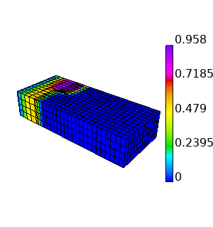
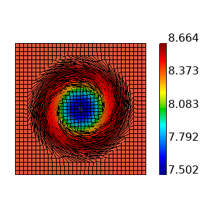
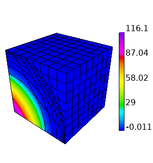
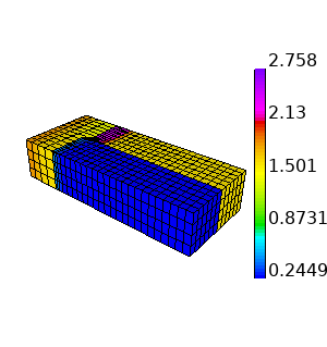
Fig. 1: Visualization of final-time velocity (top) and energy (bottom) on the Lagrangian frame for long-time FOM simulation in various benchmark problems: the Gresho vortex problem (first column), the Sedov Blast problem (second column), the Taylor–Green vortex problem (third column) and the triple–point problem (fourth column).

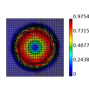
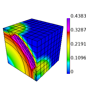
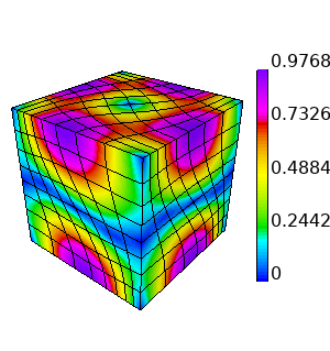
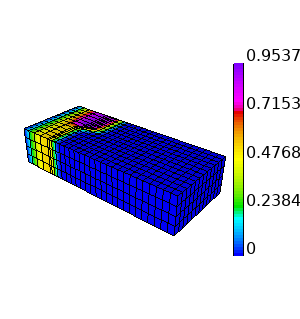
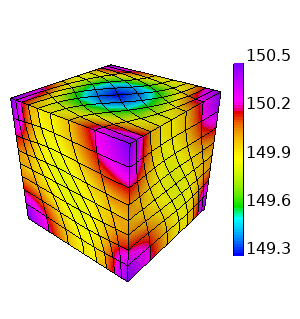
Fig. 2: Visualization of final-time velocity (top) and energy (bottom) on the Lagrangian frame for long-time ROM simulation in various benchmark problems: the Gresho vortex problem (first column), the Sedov Blast problem (second column), the Taylor–Green vortex problem (third column) and the triple–point problem (fourth column).

6.2 Short-time ROM simulation

In this section, we use the spatial ROM introduced in Section 3 to perform short-time simulation in various benchmark problems. Only reproductive cases are considered, i.e. the problem setting in the ROM is identical to that in the FOM. First, in the offline phase, the fully discrete FOM scheme in Section 2.2 is used to compute snapshot solution for performing POD discussed in Section 3.5. The reduced basis matrices for the solution variables are then used to formulate the reduced order model (3.8) in the online phase. In the case of hyper-reduction, we also obtain the reduced basis matrices for the nonlinear terms using SVD or the SNS relation, and then follow the DEIM procedure discussed in Section 3.7 to obtain sampling matrices and formulate the hyper-reduced system (3.17). Using a time integrator again, the fully discrete (hyper-)reduced order model is used to compute an approximate solution. The ROM solution is compared with the FOM solution at the final time $t_{f}$ with respect to the relative errors (6.1). Also, the wall time of ROM simulation is compared with that of the FOM simulation. We will study the dependence of the accuracy and speed-up of ROM on the ratios of dimension reduction

(6.9) $$\zeta_{v}=\dfrac{n_{v}}{N_{\mathcal{V}}},\quad\zeta_{e}=\dfrac{n_{e}}{N_{\mathcal{E}}},\quad\zeta_{x}=\dfrac{n_{x}}{N_{\mathcal{V}}},\quad\zeta_{\breve{\mathsf{F}^{\mathfrak{1}}}}=\dfrac{n_{\breve{\mathsf{F}^{\mathfrak{1}}}}}{N_{\mathcal{V}}},\quad\zeta_{\breve{\mathsf{F}^{tv}}}=\dfrac{n_{\breve{\mathsf{F}^{tv}}}}{N_{\mathcal{E}}}.$$

On the other hand, for hyper-reduction, the numbers of sampling indices $\{n_{\breve{\mathsf{F}^{\mathfrak{1}}}},n_{\breve{\mathsf{F}^{tv}}}\}$ are controlled by the product of the over-sampling factors $\{\lambda_{\breve{\mathsf{F}^{\mathfrak{1}}}},\lambda_{\breve{\mathsf{F}^{tv}}}\}\in[1,\infty)$ and the reduced basis dimensions $\{n_{\mathsf{F}^{\mathfrak{1}}},n_{\mathsf{F}^{tv}}\}$, i.e.

(6.10) $$n_{\breve{\mathsf{F}^{\mathfrak{1}}}}=\min\left\{N_{\mathcal{V}},\,\lambda_{\breve{\mathsf{F}^{\mathfrak{1}}}}n_{\mathsf{F}^{\mathfrak{1}}}\right\},\quad n_{\breve{\mathsf{F}^{tv}}}=\min\left\{N_{\mathcal{E}},\,\lambda_{\breve{\mathsf{F}^{tv}}}n_{\mathsf{F}^{tv}}\right\}.$$

The resultant reduced system of semi-discrete Lagrangian hydrodynamics equations is numerically solved by the RK2-average scheme introduced in Section 3.4.

In Figure 3, we compare the ROM performance on the short-time simulation in the Gresho vortex problem against reduced basis dimensions. This comparison examines how the solution representability of the reduced order model depends on the dimensions of the POD reduced bases. To this end, we fix all other ROM parameters and do not perform hyper-reduction, to avoid complicating the results. Table 2 shows the reduced basis dimensions being tested and their ratios to the dimensions of the corresponding FOM finite element spaces. From Figure 3, we see that the relative errors are overall decreasing with the reduced basis dimensions, and the accuracy is very outstanding even when low dimensional subspaces are used. However, since the nonlinear terms scale with the FOM size, the speed-up achieved is only around 1.4 for all the cases tested. This highlights the need of hyper-reduction for the sake of remarkable speed-up.

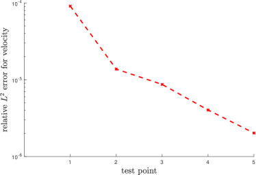
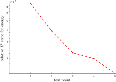
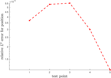
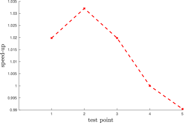
Fig. 3: ROM performance comparison for short-time simulation in the Gresho vortex problem with varying ratio of reduced basis dimensions: relative $L^{2}$ error for velocity (top-left), relative $L^{2}$ error for energy (top-right), relative $L^{2}$ error for position (bottom-left) and speed-up (bottom-right). Table 2 provides test points.

Test point	1	2	3	4	5
$n_{v}$	6	11	17	23	28
$n_{e}$	9	18	27	36	44
$n_{x}$	2	4	6	8	10
$\zeta_{v}$	0.000318844	0.000584547	0.00090339	0.00122223	0.00148794
$\zeta_{e}$	0.000976562	0.00195312	0.00292969	0.00390625	0.00477431
$\zeta_{x}$	0.000106281	0.000212562	0.000318844	0.000425125	0.000531406

Table 2: List of reduced basis dimensions being tested in Figure 3 and their ratio to the dimensions of the corresponding FOM finite element spaces for short-time simulation in the Gresho vortex problem.

In Figure 4, we compare the ROM performance on the short-time simulation in the Gresho vortex problem against the number of sampling indices. This comparison examines how the solution accuracy depends on the projection error of the nonlinear terms in the DEIM nonlinear model reduction. We compare different approaches for obtaining the nonlinear term bases, i.e. directly applying snapshot SVD and using the SNS relation [13]. To avoid complicating the results with respect to different ROM parameters, we fix the reduced basis dimensions as $(n_{v},n_{e},n_{x},n_{\mathsf{F}^{\mathfrak{1}}},n_{\mathsf{F}^{tv}})=(28,44,10,28,44)$. We also compare different algorithms for obtaining the sampling indices, namely the over-sampling DEIM (see Algorithm 3 of [81] and Algorithm 5 of [82]) and QDEIM (see [79]). Table 3 shows the number of sampling indices being tested and their ratio to the dimensions of the corresponding FOM finite element spaces. From Figure 4, we see that the relative errors and speed-up are overall decreasing with the number of sampling indices, while the accuracy is still remarkable for each of the nonlinear model reduction technique. We remark that the first test point with DEIM has a numerical instability as the time step size eventually vanishes. In this experiment, we observe that SNS-DEIM has the highest accuracy and best speed-up compared with the other approaches. In the rest of the paper, unless otherwise specified, we will mainly focus on the SNS-DEIM approach as suggested by this experiment.

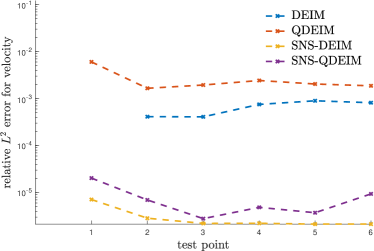
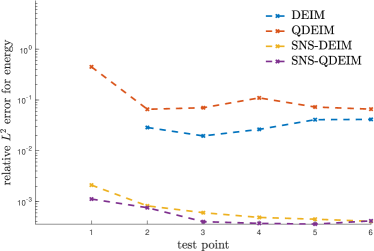
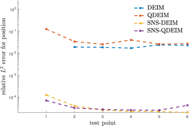
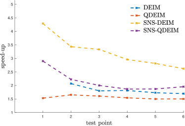
Fig. 4: ROM performance comparison for short-time simulation in the Gresho vortex problem with varying ratio of sampling indices: relative $L^{2}$ error for velocity (top-left), relative $L^{2}$ error for energy (top-right), relative $L^{2}$ error for position (bottom-left) and speed-up (bottom-right). Table 3 provides test points.

Test point	1	2	3	4	5	6
$\lambda_{\breve{\mathsf{F}^{\mathfrak{1}}}}$	8	15	23	30	37	45
$\lambda_{\breve{\mathsf{F}^{tv}}}$	7	14	21	28	35	41
$n_{\breve{\mathsf{F}^{\mathfrak{1}}}}$	616	1232	1848	2464	3080	3696
$n_{\breve{\mathsf{F}^{tv}}}$	396	792	1188	1584	1980	2376
$\zeta_{\breve{\mathsf{F}^{\mathfrak{1}}}}$	0.0327346	0.0654692	0.0982038	0.130938	0.163673	0.196408
$\zeta_{\breve{\mathsf{F}^{tv}}}$	0.0429688	0.0859375	0.128906	0.171875	0.214844	0.257812

Table 3: List of number of sampling indices being tested in Figure 4 and their ratio to the dimensions of the corresponding FOM finite element spaces for short-time simulation in the Gresho vortex problem.

Table 4 shows the short-time numerical results using SNS-DEIM spatial ROM for various benchmark problems. The quantities reported in Table 4 include

• the final time $t_{f}$ and the number of time steps $N_{t}$ in the FOM simulations,

• the ROM user-defined input values, namely the threshold $\epsilon_{\sigma}$ and the over-sampling factors $\{\lambda_{\breve{\mathsf{F}^{\mathfrak{1}}}},\lambda_{\breve{\mathsf{F}^{tv}}}\}$,

• the ROM parameters, namely the reduced dimensions $\{n_{v},n_{e},n_{x}\}$ (note that with our SNS setting, we have $n_{\mathsf{F}^{\mathfrak{1}}}=n_{v}$ and $n_{\mathsf{F}^{tv}}=n_{e}$) and the number of sampling indices $\{n_{\breve{\mathsf{F}^{\mathfrak{1}}}},n_{\breve{\mathsf{F}^{tv}}}\}$, and

• the ROM results, namely the number of time steps $\widetilde{N}_{t}$ in the ROM simulations, the relative errors $\{\mathcal{\epsilon}_{v,t_{f}},\mathcal{\epsilon}_{e,t_{f}},\mathcal{\epsilon}_{x,t_{f}}\}$ at the final time, and the relative speed-up of the ROM simulations to FOM simulations.

In each of the benchmark problems, it can be observed that the number of time steps $\widetilde{N}_{t}$ in the ROM simulations is close to but slightly differ from $N_{t}$ in the FOM simulations. The ROM simulation benefits from the relatively cheap reduced dimension computation in each time step to achieve an overall relative speed-up. The relative error is small for each variable, indicating that the ROM solutions provide accurate approximations to the FOM solutions.

Problem	Gresho vortex	Sedov Blast	Taylor–Green vortex	Triple–point
$t_{f}$	0.1	0.1	0.05	0.2
$N_{t}$	87	245	122	28
$\epsilon_{\sigma}$	0.9999	0.9999	0.9999	0.9999
$\lambda_{\breve{\mathsf{F}^{\mathfrak{1}}}}$	8	2	2	2
$\lambda_{\breve{\mathsf{F}^{tv}}}$	8	2	2	2
$n_{v}$	32	53	9	10
$n_{e}$	72	13	16	10
$n_{x}$	10	17	3	7
$n_{\breve{\mathsf{F}^{\mathfrak{1}}}}$	256	106	18	20
$n_{\breve{\mathsf{F}^{tv}}}$	576	26	32	20
$\widetilde{N}_{t}$	87	225	122	29
$\mathcal{\epsilon}_{v,t_{f}}$	1.385366e-02	2.74144e-03	9.05004e-05	9.41694e-03
$\mathcal{\epsilon}_{e,t_{f}}$	2.02558e-03	8.39586e-04	3.69690e-06	4.91346e-03
$\mathcal{\epsilon}_{x,t_{f}}$	1.76761e-04	2.04953e-05	6.81088e-07	4.03934e-05
speed-up	8.27130	26.55553	14.75786	53.02794

Table 4: FOM results, ROM user-defined input values, parameters and results for short-time simulation in various benchmark problems.

6.3 Long-time ROM simulation

In this section, we use the spatial ROM introduced in Section 3 and the time-windowing ROM introduced in Section 4 to perform long-time simulation in various benchmark problems. Again, only reproductive cases are considered. For the spatial ROM, we use SNS-DEIM for hyper-reduction and the offline-online procedure splitting is the same as in Section 6.2. Table 5 shows the long-time numerical results using SNS-DEIM spatial ROM for various benchmark problems. It can be observed that the relative errors are still reasonable, but the relative speed-up is lower than that in the short-time simulations. In these simulations, large over-sampling factors $\{\lambda_{\breve{\mathsf{F}^{\mathfrak{1}}}},\lambda_{\breve{\mathsf{F}^{tv}}}\}$ are used to maintain sufficient numbers of sampling indices $\{n_{\breve{\mathsf{F}^{\mathfrak{1}}}},n_{\breve{\mathsf{F}^{tv}}}\}$, for otherwise the time step size would eventually vanish due to the adaptive time stepping control and the CFL constraints. However, larger numbers of sampling indices lead to more expensive overdetermined systems (3.13) and (3.15) for the hyper-reduction and hurt the overall speed-up in ROM simulations. It is especially important to point out that the spatial ROM does not achieve a speed-up in the Gresho vortex problem since more reduced basis vectors are required to ensure the solution representability of the reduced linear space, and almost full sampling has to be used for the sake of numerical stability.

Problem	Gresho vortex	Sedov Blast	Taylor–Green vortex	Triple–point
$t_{f}$	0.62	0.8	0.25	0.8
$N_{t}$	1672	719	897	193
$\epsilon_{\sigma}$	0.9999	0.9999	0.9999	0.9999
$\lambda_{\breve{\mathsf{F}^{\mathfrak{1}}}}$	100	6	80	6
$\lambda_{\breve{\mathsf{F}^{tv}}}$	100	6	40	6
$n_{v}$	165	225	40	20
$n_{e}$	331	27	62	16
$n_{x}$	34	29	6	10
$n_{\breve{\mathsf{F}^{\mathfrak{1}}}}$	16500	1350	3200	120
$n_{\breve{\mathsf{F}^{tv}}}$	9216	162	2480	96
$\widetilde{N}_{t}$	1670	742	898	193
$\mathcal{\epsilon}_{v,t_{f}}$	4.29468e-02	9.72044e-03	3.60272e-02	2.52978e-03
$\mathcal{\epsilon}_{e,t_{f}}$	6.82899e-03	5.95163e-04	3.28395e-03	2.36835e-03
$\mathcal{\epsilon}_{x,t_{f}}$	7.1045e-05	3.67286e-04	2.77386e-04	4.72467e-05
speed-up	0.79646	3.35523	1.96808	15.29550

Table 5: FOM results, ROM user-defined input values, parameters and results for long-time simulation in various benchmark problems.

Next, we examine the performance of the time windowing ROM approach. In our implementation, the end points of the time windows $\{T_{w}\}_{w=1}^{N_{w}}$ can either be determined by physical time as in Section 4.4.1, or by the number of samples as in Section 4.4.2. We focus our discussion on the SNS-DEIM time windowing ROM approach with the end points of the time windows determined by the number of samples. In the offline phase, the fully discrete RK2-average FOM scheme is first used to compute solution snapshots. The time windows are determined according to (4.21). Following Section 4.5, the collected solution data are clustered into different windows for performing POD, and the resultant reduced solution bases for velocity and energy are left-multiplied by the corresponding mass matrix to obtain the nonlinear term bases, which in turn determine the sampling indices by DEIM. In the online phase, the reduced basis matrices and the sampling matrices are then used to formulate the hyper-reduced system (4.10) in each time window. The fully discrete hyper-reduced system follows from applying the RK2-average scheme as discussed in Section 3.4.

Table 6 shows the long-time numerical results for various benchmark problems with time windowing ROM. In the case of decomposing time windows by number of samples, the number of time windows $N_{w}$ is an additional ROM parameter controlled by the number of samples per window $N_{\text{sample}}$ as an additional user-defined input. We use $N_{\text{sample}}=10$ in each of the benchmark problems. Moreover, in our implementation, the over-sampling factors $\{\lambda_{\breve{\mathsf{F}^{\mathfrak{1}}}},\lambda_{\breve{\mathsf{F}^{tv}}}\}$ are user-defined constants over all time windows, which control the number of sampling indices in the window $w$ by

(6.11) $$n_{\breve{\mathsf{F}^{\mathfrak{1}}}}^{w}=\min\left\{N_{\mathcal{V}},\,\lambda_{\breve{\mathsf{F}^{\mathfrak{1}}}}n_{\mathsf{F}^{\mathfrak{1}}}^{w}\right\},\quad n_{\breve{\mathsf{F}^{tv}}}^{w}=\min\left\{N_{\mathcal{E}},\,\lambda_{\breve{\mathsf{F}^{tv}}}n_{\mathsf{F}^{tv}}^{w}\right\}.$$

In Table 6, the reported values of reduced basis dimensions and the number of sampling indices are taken as the greatest among all windows, i.e.

(6.12) $$n_{v}=\max_{1\leq w\leq N_{w}}n_{v}^{w},\quad n_{e}=\max_{1\leq w\leq N_{w}}n_{e}^{w},\quad n_{x}=\max_{1\leq w\leq N_{w}}n_{x}^{w},\quad n_{\breve{\mathsf{F}^{\mathfrak{1}}}}=\max_{1\leq w\leq N_{w}}n_{\breve{\mathsf{F}^{\mathfrak{1}}}}^{w},\quad n_{\breve{\mathsf{F}^{tv}}}=\max_{1\leq w\leq N_{w}}n_{\breve{\mathsf{F}^{tv}}}^{w}.$$

It can be observed from comparing Table 6 with Table 5 that it is possible to achieve a higher relative speed-up and improve solution accuracy using time windowing ROM. In particular, for the Gresho vortex problem, when the spatial ROM fails to achieve any relative speed-up, the time windowing approach yields relative error or order $10^{-6}$ in all solution variables and a $25$ times speed-up. This suggests that the time windowing approach is more useful for the advection-dominated cases, in which the intrinsic dimensions of reduced subspaces in the spatial ROM are large.

Problem	Gresho vortex	Sedov Blast	Taylor–Green vortex	Triple–point
$t_{f}$	0.62	0.8	0.25	0.8
$N_{t}$	1672	719	897	193
$N_{\text{sample}}$	10	10	10	10
$\epsilon_{\sigma}$	0.9999	0.9999	0.9999	0.9999
$\lambda_{\breve{\mathsf{F}^{\mathfrak{1}}}}$	2	2	2	2
$\lambda_{\breve{\mathsf{F}^{tv}}}$	2	2	2	2
$N_{w}$	335	144	180	39
$n_{v}$	8	10	3	7
$n_{e}$	10	7	5	8
$n_{x}$	6	7	2	5
$n_{\breve{\mathsf{F}^{\mathfrak{1}}}}$	16	20	6	14
$n_{\breve{\mathsf{F}^{tv}}}$	20	14	10	16
$\widetilde{N}_{t}$	1599	697	897	155
$\mathcal{\epsilon}_{v,t_{f}}$	3.50163e-06	4.58111e-04	1.22769e-06	9.31072e-04
$\mathcal{\epsilon}_{e,t_{f}}$	3.51595e-07	2.95541e-05	5.35795e-08	6.99656e-04
$\mathcal{\epsilon}_{x,t_{f}}$	4.28729e-07	3.86835e-05	6.95479e-09	3.82897e-05
speed-up	24.59098	26.47649	23.46642	75.03020

Table 6: FOM results, time windowing ROM user-defined input values, parameters and results for long-time simulation in various benchmark problems.

At the end of this subsection, we compare the performance of the ROM approach with SNS-DEIM across different window size on long-time simulation in the Gresho vortex problem and the Sedov Blast problem. We will consider the spatial ROM in Section 3 and the time windowing ROM in Section 4. The endpoints of the time windows $\{T_{w}\}_{w=1}^{N_{w}}$ are determined by (4.21) with the number of samples $N_{\text{sample}}$. More precisely, the cases under consideration in the Gresho vortex problem are:

• $N_{w}=1$ corresponds to serial ROM,

• $N_{\text{sample}}=10$ corresponds to time windowing ROM which generates $N_{w}=335$ time windows, and

• $N_{\text{sample}}=20$ corresponds to time windowing ROM which generates $N_{w}=168$ time windows, and

• $N_{\text{sample}}=40$ corresponds to time windowing ROM which generates $N_{w}=84$ time windows.

Meanwhile, the cases under consideration in the Sedov Blast problem are:

• $N_{w}=1$ corresponds to serial ROM,

• $N_{\text{sample}}=10$ corresponds to time windowing ROM which generates $N_{w}=144$ time windows, and

• $N_{\text{sample}}=20$ corresponds to time windowing ROM which generates $N_{w}=72$ time windows, and

• $N_{\text{sample}}=40$ corresponds to time windowing ROM which generates $N_{w}=36$ time windows.

Depending on the reduced dimensions $\{n_{\mathsf{F}^{\mathfrak{1}}},n_{\mathsf{F}^{tv}}\}$ of the nonlinear term bases, each case is tested with various combinations of over-sampling factors $(\lambda_{\breve{\mathsf{F}^{\mathfrak{1}}}},\lambda_{\breve{\mathsf{F}^{tv}}})$ to obtain adjustable solution accuracy and speed-up.

For each of the problems, we construct a Pareto front in Figure 5 for each of the cases, which is characterized by the ROM user-defined input values that minimize the competing objectives of relative $L^{2}$ error for velocity and relative wall time. An overall Pareto front that selects the ROM parameters that are Pareto-optimal across all groups is also illustrated for each problem. Table 7 reports the ROM user-defined input values that yielded the results on the overall Pareto front. The results also suggest that the time windowing approaches can produce a remarkable speed-up as well as accurate approximations with the appropriate use of hyper-reduction.

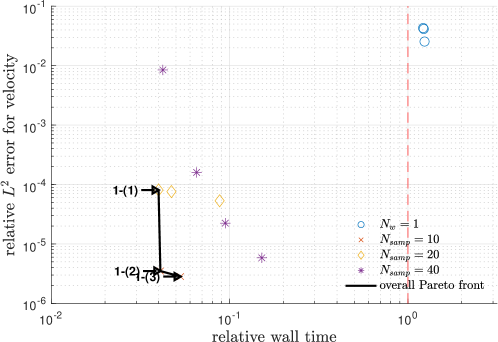
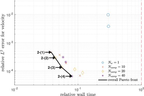
Fig. 5: ROM performance comparison for long-time simulation in the Gresho vortex problem (top) and the Sedov Blast problem (bottom). Relative $L^{2}$ error for velocity versus relative wall time for varying ROM parameters.

Label	1-(1)	1-(2)	1-(3)	2-(1)	2-(2)	2-(3)	2-(4)
$N_{w}$	–	–	–	–	–	–	–
$N_{\text{sample}}$	20	20	10	10	20	20	40
$\epsilon_{\sigma}$	0.9999	0.9999	0.9999	0.9999	0.9999	0.9999	0.9999
$\lambda_{\breve{\mathsf{F}^{\mathfrak{1}}}}$	2	2	4	2	2	4	8
$\lambda_{\breve{\mathsf{F}^{tv}}}$	2	2	4	2	2	4	8

Table 7: ROM user-defined input values yielding Pareto-optimal performance for long-time simulation in the Gresho vortex problem and the Sedov Blast problem. Figure 5 provides labels.

6.4 Parametric ROM simulation

In this section, we use the time-windowing ROM introduced in Section 4 to perform long-time simulation in the Sedov Blast problem in a parametric problem setting. In our numerical experiments, the initial internal energy deposited at the origin is parametrized by the problem parameter $\boldsymbol{\mu}\in\mathsf{D}=\mathbb{R}^{+}$, where we set $e(0,0,0;\boldsymbol{\mu})=0.25\boldsymbol{\mu}$. First, in the offline phase, the fully discrete FOM scheme is used to compute snapshot solution with several problem parameters $\{\boldsymbol{\mu}_{k}\}_{k=1}^{n_{\mu}}$. Then, we consider the SNS-DEIM time windowing ROM approach with the end points of the time windows determined by number of samples as in Section 4.4.2.

The FOM solutions with $n_{\mu}=3$ problem parameters, namely $\{\boldsymbol{\mu}_{1},\boldsymbol{\mu}_{2},\boldsymbol{\mu}_{3}\}=\{0.8,1.0,1.2\}$, are computed and collected as snapshots for determining the time windows. Then POD and SNS-DEIM are performed in each window using each choice of the offset vectors as discussed in Section 4.6. The time windows are determined according to (4.21) with $N_{\text{sample}}=20$. Then the ROM is tested on a generic problem parameter $\boldsymbol{\mu}$, where the offset vectors $\boldsymbol{v}_{\text{os}}^{w}(\boldsymbol{\mu}),\boldsymbol{e}_{\text{os}}^{w}(\boldsymbol{\mu}),\boldsymbol{x}_{\text{os}}^{w}(\boldsymbol{\mu})$ are computed in each of the time windows $w$ according to the choice of offset vectors used in constructing the solution bases. In Figure 6, we compare the ROM performance on the long-time simulation in the Sedov Blast problem against the generic problem parameter $\boldsymbol{\mu}\in[0.7,1.3]$. This comparison examines how the solution representability of the reduced order model depends on the problem parameter and the choice of offset vectors. To this end, we fix all other ROM parameters and do not perform hyper-reduction to avoid complicating the results. The comparison is also made against the spatial ROM. As shown in Figure 6, the time windowing approach provides a much better speed-up than the serial ROM. We also remark that the serial ROM has a numerical instability in $\boldsymbol{\mu}\in\{1.2,1.3\}$ as the time step size eventually vanishes, which we do not see in the time windowing ROM. We can observe from Figure 6 that using the interpolation scheme in Section 4.6.3 outperforms the other approaches of computing offset vectors in terms of the relative errors in the reproductive cases $\boldsymbol{\mu}\in\{0.8,1.0,1.2\}$, at which the offset vectors are exactly the interpolating values for each time window. However, this approach produces larger error at the predictive cases. This suggests that the error of offset determination by the interpolation scheme plays a crucial part in the final-time error. On the other hand, using the the initial state as offset vectors, which is described in Section 4.6.1, provides uniformly improved accuracy when compared with serial ROM. Moreover, it provides a speed-up of around 15 times at all the tested parameter values, which outperforms the interpolation scheme.

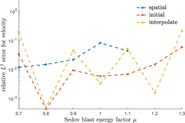
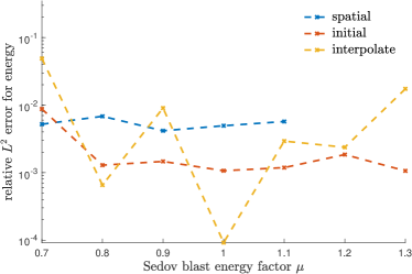
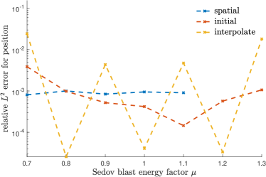
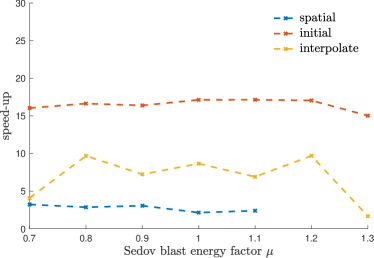
Fig. 6: Time-windowing ROM performance comparison for long-time simulation in the parametric Sedov Blast problem with varying problem parameter: relative $L^{2}$ error for velocity (top-left), relative $L^{2}$ error for energy (top-right), relative $L^{2}$ error for position (bottom-left) and speed-up (bottom-right).

At the end of this subsection, we compare the performance of various parametric time windowing ROM approaches across a wide variation of all ROM parameters on long-time simulation in the Sedov Blast problem in the setting of varying the energy factor. The FOM solutions with $n_{\mu}=3$ problem parameters, namely $\{\boldsymbol{\mu}_{1},\boldsymbol{\mu}_{2},\boldsymbol{\mu}_{3}\}=\{0.8,1.0,1.2\}$, are computed and collected as snapshots for determining the time windows, and then performing POD and SNS-DEIM in each window using each choice of the offset vectors as discussed in Section 4.6. The time windows are determined according to (4.21) with $N_{\text{sample}}=20$. The ROM performance is tested on the problem parameters $\boldsymbol{\mu}\in\{0.7,0.8,0.9\}$. Again, we compare different choices of the offset vectors as discussed in Section 4.6, and the comparison is also made against the spatial ROM. Depending on the reduced dimensions $\{n_{\mathsf{F}^{\mathfrak{1}}},n_{\mathsf{F}^{tv}}\}$ of the nonlinear term bases, each case is tested with various combinations of over-sampling factors $(\lambda_{\breve{\mathsf{F}^{\mathfrak{1}}}},\lambda_{\breve{\mathsf{F}^{tv}}})$ to obtain adjustable solution accuracy and speed-up.

We remark that the tested parameter $\boldsymbol{\mu}=0.8$ is a reproductive case, the tested parameter $\boldsymbol{\mu}=0.9$ is a predictive case in the interpolation regime, while the case $n_{\mu}=0.7$ is predictive in the extrapolation regime. For each of the tested problem parameters $\boldsymbol{\mu}\in\{0.7,0.8,0.9\}$, we construct a Pareto front in Figure 7 for each of the cases, which is characterized by the ROM user-defined input values that minimize the competing objectives of relative $L^{2}$ error for velocity and relative wall time. An overall Pareto front that selects the ROM parameters that are Pareto-optimal across all groups is also illustrated for each problem. Table 8 reports the ROM user-defined input values that yielded the results on the overall Pareto front. The numerical results show that for the predictive cases $\boldsymbol{\mu}\in\{0.7,0.9\}$, using the initial state as offset vectors described in Section 4.6.1 is Pareto optimal in any region. It is also Pareto optimal for smaller relative wall time for the reproductive case $\boldsymbol{\mu}=0.8$. In larger relative wall time, using the interpolation scheme in Section 4.6.3 is Pareto optimal for $\boldsymbol{\mu}=0.8$.

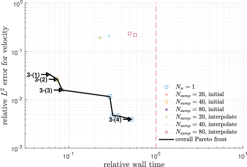
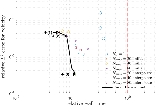
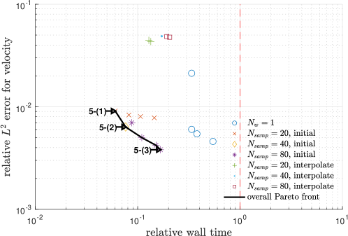
Fig. 7: ROM performance comparison for long-time simulation in the parametric Sedov Blast problem with the tested problem parameters $\boldsymbol{\mu}=0.7$ (top), $\boldsymbol{\mu}=0.8$ (mid) and $\boldsymbol{\mu}=0.9$ (bottom). Relative $L^{2}$ error for velocity versus relative wall time for varying ROM parameters.

Label	3-(1)	3-(2)	3-(3)	3-(4)	4-(1)	4-(2)	4-(3)	5-(1)	5-(2)	5-(3)
$N_{w}$	–	–	–	1	–	–	–	–	–	–
$N_{\text{sample}}$	20	40	80	–	20	80	20	20	40	80
$\epsilon_{\sigma}$	0.9999	0.9999	0.9999	0.9999	0.9999	0.9999	0.9999	0.9999	0.9999	0.9999
Offset	Initial	Initial	Initial	–	Initial	Initial	Interpolate	Initial	Initial	Initial
$\lambda_{\breve{\mathsf{F}^{\mathfrak{1}}}}$	4	4	4	32	4	4	8	4	4	32
$\lambda_{\breve{\mathsf{F}^{tv}}}$	4	4	4	32	4	4	8	4	4	32

Table 8: ROM user-defined input values yielding Pareto-optimal performance for long-time simulation in the parametric Sedov Blast problem. Figure 7 provides labels.

7 Conclusion

In this paper, we develop an efficient reduced order modeling approach for Lagrangian hydrodynamics simulations. A time-windowing approach is introduced to construct temporally-local ROM spaces which are small but accurate within a short period in advection-dominated problems. Different techniques of window division and construction of offset variables are discussed. Over-sampling hyper-reduction on the nonlinear terms are introduced to ensure adequate speed-up. Error bounds for the fully discrete reduced order model with adaptive time-step control are developed using the continuous-in-time full order model solution as the reference. The error bounds are controlled by several quantities, including the oblique projection error of the solution and the nonlinear terms onto reduced subspaces, the mismatch of initial condition, an exponential factor of the time of evaluation, and the maximum time step size. Numerical examples are shown to verify the capability of our method. For the long-time simulation in benchmark advection-dominated problems, the time windowing reduced order model successfully captures the extreme mesh distortion exhibited in the Lagrangian full order model, and attains remarkable speed-up of 25 to 75 times and outstanding solution accuracy with the order of -9 to -4 in the reproductive cases. As suggested by the numerical results, the subspace relation is useful for extracting quality nonlinear term bases and improving the solution accuracy and overall speed-up. Various offset approaches in the time windowing reduced order model are compared. In the reproductive case, using the interpolation scheme is Pareto optimal in the region of higher solution accuracy, while using the initial states is Pareto optimal in the region of smaller relative clock time. In the predictive cases, using the initial states provides uniformly improved accuracy when compared with serial ROM and a speed-up of around 15 times at all the tested parameter values.

Disclaimer

This document was prepared as an account of work sponsored by an agency of the United States government. Neither the United States government nor Lawrence Livermore National Security, LLC, nor any of their employees makes any warranty, expressed or implied, or assumes any legal liability or responsibility for the accuracy, completeness, or usefulness of any information, apparatus, product, or process disclosed, or represents that its use would not infringe privately owned rights. Reference herein to any specific commercial product, process, or service by trade name, trademark, manufacturer, or otherwise does not necessarily constitute or imply its endorsement, recommendation, or favoring by the United States government or Lawrence Livermore National Security, LLC. The views and opinions of authors expressed herein do not necessarily state or reflect those of the United States government or Lawrence Livermore National Security, LLC, and shall not be used for advertising or product endorsement purposes.

Appendix A Command line options of Laghos

In this section, we present some examples of the command line options of Laghos simulation for the purpose of reproducible research. Due to rapid software development in the repository, the commands lines are subject to change. However, we try our best to present the command lines compatible with recent versions of different dependent softwares and maintain a simple usage of the program. The following command lines are compatible with the recent commits of the master branch of MFEM , the master branch of libROM , and the rom branch of Laghos . In order to use the ROM capability of Laghos, a user has to navigate to the rom subdirectory.

A.1 Problem specification

First, we present the commands lines for the FOM user-defined input values reported in Table 1 using the executable laghos. These command lines can also be used along with command line options for ROM user-defined input values. We use the long-time simulation for illustration. The command line options for specifying the Gresho vortex problem are

./laghos -p 4 -m data/square_gresho.mesh -rs 4 -ok 3 -ot 2 -tf 0.62 -s 7

The command line options for specifying the Sedov Blast problem are

./laghos -p 1 -m data/cube01_hex.mesh -pt 211 -tf 0.8 -s 7

The command line options for specifying the Taylor–Green vortex problem are

./laghos -p 0 -m data/cube01_hex.mesh -cfl 0.1 -tf 0.25 -s 7

The command line options for specifying the triple–point problem are

./laghos -p 3 -m data/box01_hex.mesh -tf 0.8 -s 7

A.2 Long-time serial ROM simulation

Next, we present the command line options for the long-time serial ROM simulation in the Sedov Blast problem reported in the second column of Table 5. The options are appended to the command lines for specifying the Sedov Blast problem in Section A.1. The other problems in Table 5 can be simulated using similar options. For computing FOM reference solution, snapshot sampling and basis generation in the offline phase, one appends

-offline -writesol -romsns -ef 0.9999 -sample-stages

For hyper-reduction preprocessing in the online phase, one appends

-online -romhrprep -romsns -rdimv 225 -rdime 27 -rdimx 29 -sfacv 6 -sface 6

For ROM simulation in the online phase, one appends

-online -romhr -romsns -rdimv 225 -rdime 27 -rdimx 29 -sfacv 6 -sface 6

Finally, for solution postprocessing and calculating the relative error, one appends

-restore -soldiff -romsns -rdimv 225 -rdime 27 -rdimx 29

A.3 Long-time time windowing ROM simulation

Next, we present the command line options for the long-time time windowing ROM simulation in the Sedov Blast problem reported in the second column of Table 6. The options are appended to the command lines for specifying the Sedov Blast problem in Section A.1. The other problems in Table 6 can be simulated using similar options. For computing FOM reference solution, snapshot sampling and basis generation in the offline phase, one appends

-offline -writesol -romsns -ef 0.9999 -sample-stages -nwinsamp 10 -rostype load

For hyper-reduction preprocessing in the online phase, one appends

-online -romhrprep -romsns -sfacv 2 -sface 2 -nwin 144 -rostype load

For ROM simulation in the online phase, one appends

-online -romhr -romsns -sfacv 2 -sface 2 -nwin 144 -rostype load

Finally, for solution postprocessing and calculating the relative error, one appends

-restore -soldiff -romsns -nwin 144 -rostype load

A.4 Parametric time windowing ROM simulation

Finally, we present the command line options for the long-time time windowing ROM simulation in the parametric Sedov Blast problem reported in the Label 4-(1) of Table 8. The options are appended to the command lines for specifying the Sedov Blast problem in Section A.1, except that for the basis generation a separate executable merge is used. The other labels in Table 8 can be simulated using similar options. For computing FOM reference solution with $\boldsymbol{\mu}=0.8$ and snapshot sampling in the offline phase, one appends

-offline -romsns -bef 1.0 -rpar 0 -sample-stages -rostype initial
-offline -romsns -bef 1.2 -rpar 1 -sample-stages -rostype initial
-offline -romsns -bef 0.8 -rpar 2 -sample-stages -rostype initial -writesol

For basis generation in the offline phase of the parametric problem, one uses a separate executable merge

./merge -nset 3 -romsns -ef 0.9999 -nwinsamp 20 -rostype initial

For hyper-reduction preprocessing in the online phase, one appends

-online -romhrprep -romsns -bef 0.8 -sfacv 4 -sface 4 -nwin 80 -rostype initial

For ROM simulation in the online phase, one appends

-online -romhr -romsns -bef 0.8 -sfacv 4 -sface 4 -nwin 80 -rostype initial

Finally, for solution postprocessing and calculating the relative error, one appends

-restore -soldiff -romsns -nwin 80 -rostype initial

References

- [1] Shun Wang, Eric de Sturler, and Glaucio H Paulino. Large-scale topology optimization using preconditioned Krylov subspace methods with recycling. International journal for numerical methods in engineering, 69(12):2441–2468, 2007.
- [2] Miguel A Salazar de Troya and Daniel A Tortorelli. Three-dimensional adaptive mesh refinement in stress-constrained topology optimization. Structural and Multidisciplinary Optimization, 62(5):2467–2479, 2020.
- [3] Miguel A Salazar De Troya and Daniel A Tortorelli. Adaptive mesh refinement in stress-constrained topology optimization. Structural and Multidisciplinary Optimization, 58(6):2369–2386, 2018.
- [4] Daniel A White, Youngsoo Choi, and Jun Kudo. A dual mesh method with adaptivity for stress-constrained topology optimization. Structural and Multidisciplinary Optimization, 61(2):749–762, 2020.
- [5] Youngsoo Choi, Charbel Farhat, Walter Murray, and Michael Saunders. A practical factorization of a Schur complement for PDE-constrained distributed optimal control. Journal of Scientific Computing, 65(2):576–597, 2015.
- [6] Youngsoo Choi. Simultaneous analysis and design in PDE-constrained optimization. PhD thesis, Stanford University, 2012.
- [7] Ralph C Smith. Uncertainty quantification: theory, implementation, and applications, volume 12. Siam, 2013.
- [8] Lorenz Biegler, George Biros, Omar Ghattas, Matthias Heinkenschloss, David Keyes, Bani Mallick, Luis Tenorio, Bart van Bloemen Waanders, Karen Willcox, and Youssef Marzouk. Large-scale inverse problems and quantification of uncertainty, volume 712. John Wiley & Sons, 2011.
- [9] David Galbally, Krzysztof Fidkowski, Karen Willcox, and Omar Ghattas. Non-linear model reduction for uncertainty quantification in large-scale inverse problems. International journal for numerical methods in engineering, 81(12):1581–1608, 2010.
- [10] Chi Hoang, Youngsoo Choi, and Kevin Carlberg. Domain-decomposition least-squares Petrov-Galerkin (DD-LSPG) nonlinear model reduction. arXiv preprint arXiv:2007.11835, 2020.
- [11] Felix Fritzen, Bernard Haasdonk, David Ryckelynck, and Sebastian Schöps. An algorithmic comparison of the hyper-reduction and the discrete empirical interpolation method for a nonlinear thermal problem. Mathematical and computational applications, 23(1):8, 2018.
- [12] Youngsoo Choi and Kevin Carlberg. Space–time least-squares Petrov–Galerkin projection for nonlinear model reduction. SIAM Journal on Scientific Computing, 41(1):A26–A58, 2019.
- [13] Youngsoo Choi, Deshawn Coombs, and Robert Anderson. SNS: a solution-based nonlinear subspace method for time-dependent model order reduction. SIAM Journal on Scientific Computing, 42(2):A1116–A1146, 2020.
- [14] Kevin Carlberg, Youngsoo Choi, and Syuzanna Sargsyan. Conservative model reduction for finite-volume models. Journal of Computational Physics, 371:280–314, 2018.
- [15] Rambod Mojgani and Maciej Balajewicz. Lagrangian basis method for dimensionality reduction of convection dominated nonlinear flows. arXiv preprint arXiv:1701.04343, 2017.
- [16] Youngkyu Kim, Karen May Wang, and Youngsoo Choi. Efficient space-time reduced order model for linear dynamical systems in Python using less than 120 lines of code. arXiv preprint arXiv:2011.10648, 2020.
- [17] Dunhui Xiao, Fangxin Fang, Andrew G Buchan, Christopher C Pain, Ionel Michael Navon, Juan Du, and G Hu. Non-linear model reduction for the navier–Stokes equations using residual deim method. Journal of Computational Physics, 263:1–18, 2014.
- [18] John Burkardt, Max Gunzburger, and Hyung-Chun Lee. POD and CVT-based reduced-order modeling of Navier–Stokes flows. Computer methods in applied mechanics and engineering, 196(1-3):337–355, 2006.
- [19] David Amsallem, Matthew Zahr, Youngsoo Choi, and Charbel Farhat. Design optimization using hyper-reduced-order models. Structural and Multidisciplinary Optimization, 51(4):919–940, 2015.
- [20] Youngsoo Choi, Gabriele Boncoraglio, Spenser Anderson, David Amsallem, and Charbel Farhat. Gradient-based constrained optimization using a database of linear reduced-order models. Journal of Computational Physics, 423:109787, 2020.
- [21] Youngsoo Choi, Geoffrey Oxberry, Daniel White, and Trenton Kirchdoerfer. Accelerating design optimization using reduced order models. arXiv preprint arXiv:1909.11320, 2019.
- [22] Sean McBane and Youngsoo Choi. Component-wise reduced order model lattice-type structure design. arXiv preprint arXiv:2010.10770, 2020.
- [23] Mohamadreza Ghasemi and Eduardo Gildin. Localized model reduction in porous media flow. IFAC-PapersOnLine, 48(6):242–247, 2015.
- [24] Rui Jiang and Louis J Durlofsky. Implementation and detailed assessment of a GNAT reduced-order model for subsurface flow simulation. Journal of Computational Physics, 379:192–213, 2019.
- [25] Yanfang Yang, Mohammadreza Ghasemi, Eduardo Gildin, Yalchin Efendiev, Victor Calo, et al. Fast multiscale reservoir simulations with pod-deim model reduction. SPE Journal, 21(06):2–141, 2016.
- [26] Min Wang, Siu Wun Cheung, Eric T. Chung, Maria Vasilyeva, and Yuhe Wang. Generalized multiscale multicontinuum model for fractured vuggy carbonate reservoirs. Journal of Computational and Applied Mathematics, 366:112370, 2020.
- [27] Huanhuan Yang and Alessandro Veneziani. Efficient estimation of cardiac conductivities via POD-DEIM model order reduction. Applied Numerical Mathematics, 115:180–199, 2017.
- [28] Hongfei Fu, Hong Wang, and Zhu Wang. POD/DEIM reduced-order modeling of time-fractional partial differential equations with applications in parameter identification. Journal of Scientific Computing, 74(1):220–243, 2018.
- [29] Pengfei Zhao, Cai Liu, and Xuan Feng. POD-DEIM based model order reduction for the spherical shallow water equations with Turkel-Zwas finite difference discretization. Journal of Applied Mathematics, 2014, 2014.
- [30] R Ştefănescu and Ionel Michael Navon. POD/DEIM nonlinear model order reduction of an ADI implicit shallow water equations model. Journal of Computational Physics, 237:95–114, 2013.
- [31] Youngsoo Choi, Peter Brown, Bill Arrighi, Roberti Anderson, and Kevin Huynh. Space-time reduced order model for large-scale linear dynamical systems with application to Boltzmann transport problems. Journal of Computational Physics, 424:109845, 2021.
- [32] M Mordhorst, Timm Strecker, D Wirtz, Thomas Heidlauf, and Oliver Röhrle. POD-DEIM reduction of computational EMG models. Journal of Computational Science, 19:86–96, 2017.
- [33] Gabriel Dimitriu, Ionel M Navon, and Răzvan Ştefănescu. Application of POD-DEIM approach for dimension reduction of a diffusive predator-prey system with allee effect. In International conference on large-scale scientific computing, pages 373–381. Springer, 2013.
- [34] Harbir Antil, Matthias Heinkenschloss, Ronald HW Hoppe, Christopher Linsenmann, and Achim Wixforth. Reduced order modeling based shape optimization of surface acoustic wave driven microfluidic biochips. Mathematics and Computers in Simulation, 82(10):1986–2003, 2012.
- [35] Ming-C Cheng. A reduced-order representation of the Schrödinger equation. AIP Advances, 6(9):095121, 2016.
- [36] Serkan Gugercin and Athanasios C Antoulas. A survey of model reduction by balanced truncation and some new results. International Journal of Control, 77(8):748–766, 2004.
- [37] Peter Benner, Serkan Gugercin, and Karen Willcox. A survey of projection-based model reduction methods for parametric dynamical systems. SIAM review, 57(4):483–531, 2015.
- [38] Changhong Mou, Birgul Koc, Omer San, Leo Rebholz, and Traian Iliescu. Data-driven variational multiscale reduced order models. arXiv preprint arXiv:2002.06457, 2020.
- [39] Eric J Parish and Karthik Duraisamy. Non-Markovian closure models for large eddy simulations using the Mori-Zwanzig formalism. Physical Review Fluids, 2(1):014604, 2017.
- [40] Mahmoud Gadalla, Marta Cianferra, Marco Tezzele, Giovanni Stabile, Andrea Mola, and Gianluigi Rozza. On the comparison of LES data-driven reduced order approaches for hydroacoustic analysis. Computers & Fluids, page 104819, 2020.
- [41] Michel Bergmann, C-H Bruneau, and Angelo Iollo. Enablers for robust POD models. Journal of Computational Physics, 228(2):516–538, 2009.
- [42] Jan Östh, Bernd R Noack, Siniša Krajnović, Diogo Barros, and Jacques Borée. On the need for a nonlinear subscale turbulence term in POD models as exemplified for a high-Reynolds-number flow over an Ahmed body. Journal of Fluid Mechanics, 747:518–544, 2014.
- [43] Joan Baiges, Ramon Codina, and Sergio Idelsohn. Reduced-order subscales for POD models. Computer Methods in Applied Mechanics and Engineering, 291:173–196, 2015.
- [44] Omer San and Romit Maulik. Extreme learning machine for reduced order modeling of turbulent geophysical flows. Physical Review E, 97(4):042322, 2018.
- [45] Hannah Lu and Daniel M Tartakovsky. Lagrangian dynamic mode decomposition for construction of reduced-order models of advection-dominated phenomena. Journal of Computational Physics, 407:109229, 2020.
- [46] Rémi Abgrall, David Amsallem, and Roxana Crisovan. Robust model reduction by -norm minimization and approximation via dictionaries: application to nonlinear hyperbolic problems. Advanced Modeling and Simulation in Engineering Sciences, 3(1):1–16, 2016.
- [47] Kevin Carlberg. Adaptive -refinement for reduced-order models. International Journal for Numerical Methods in Engineering, 102(5):1192–1210, 2015.
- [48] Eric J Parish and Kevin T Carlberg. Windowed least-squares model reduction for dynamical systems. arXiv preprint arXiv:1910.11388, 2019.
- [49] Yukiko S Shimizu and Eric J Parish. Windowed space-time least-squares Petrov-Galerkin method for nonlinear model order reduction. arXiv preprint arXiv:2012.06073, 2020.
- [50] Benjamin Peherstorfer. Model reduction for transport-dominated problems via online adaptive bases and adaptive sampling. arXiv preprint arXiv:1812.02094, 2018.
- [51] PG Constantine and G Iaccarino. Reduced order models for parameterized hyperbolic conservations laws with shock reconstruction. Center for Turbulence Research Annual Brief, 2012.
- [52] Tommaso Taddei and Lei Zhang. Space-time registration-based model reduction of parameterized one-dimensional hyperbolic PDEs. arXiv preprint arXiv:2004.06693, 2020.
- [53] Julius Reiss, Philipp Schulze, Jörn Sesterhenn, and Volker Mehrmann. The shifted proper orthogonal decomposition: A mode decomposition for multiple transport phenomena. SIAM Journal on Scientific Computing, 40(3):A1322–A1344, 2018.
- [54] Donsub Rim, Scott Moe, and Randall J LeVeque. Transport reversal for model reduction of hyperbolic partial differential equations. SIAM/ASA Journal on Uncertainty Quantification, 6(1):118–150, 2018.
- [55] G Welper. Transformed snapshot interpolation with high resolution transforms. SIAM Journal on Scientific Computing, 42(4):A2037–A2061, 2020.
- [56] Michael Kirby and Dieter Armbruster. Reconstructing phase space from PDE simulations. Zeitschrift für angewandte Mathematik und Physik ZAMP, 43(6):999–1022, 1992.
- [57] Kookjin Lee and Kevin T Carlberg. Model reduction of dynamical systems on nonlinear manifolds using deep convolutional autoencoders. Journal of Computational Physics, 404:108973, 2020.
- [58] Kookjin Lee and Kevin Carlberg. Deep conservation: A latent dynamics model for exact satisfaction of physical conservation laws. arXiv preprint arXiv:1909.09754, 2019.
- [59] Youngkyu Kim, Youngsoo Choi, David Widemann, and Tarek Zohdi. A fast and accurate physics-informed neural network reduced order model with shallow masked autoencoder. arXiv preprint arXiv:2009.11990, 2020.
- [60] Youngkyu Kim, Youngsoo Choi, David Widemann, and Tarek Zohdi. Efficient nonlinear manifold reduced order model. arXiv preprint arXiv:2011.07727, 2020.
- [61] Donsub Rim, Benjamin Peherstorfer, and Kyle T Mandli. Manifold approximations via transported subspaces: Model reduction for transport-dominated problems. arXiv preprint arXiv:1912.13024, 2019.
- [62] Donsub Rim, Luca Venturi, Joan Bruna, and Benjamin Peherstorfer. Depth separation for reduced deep networks in nonlinear model reduction: Distilling shock waves in nonlinear hyperbolic problems. arXiv preprint arXiv:2007.13977, 2020.
- [63] C. S. Peskin. The immersed boundary method. Acta Numerica, 11:479–517, 2002.
- [64] D. Boffi and L. Gastaldi. Discrete models for fluid-structure interactions: the finite element immersed boundary method. Discrete and Continuous Dynamical Systems - Series S, 9:89–107, 2016.
- [65] Siu Wun Cheung, Eric T. Chung, and Hyea Hyun Kim. A mass conservative scheme for fluid–structure interaction problems by the staggered discontinuous Galerkin method. Journal of Scientific Computing, 74:1423–1456, 2018.
- [66] P. K. Yeung. Lagrangian investigations of turbulence. Annual Review of Fluid Mechanics, 34:115–142, 2002.
- [67] B. Lüthi, A. Tsinober, and W. Kinzelbach. Lagrangian measurement of vorticity dynamics in turbulent flow. Journal of Fluid Mechanics, 528:87–118, 2005.
- [68] C. W. Hirt, A. A. Amsden, and J. L. Cook. An arbitrary Lagrangian-Eulerian computing method for all flow speeds. Journal of Computational Physics, 14:227–253, 1974.
- [69] David J. Benson. An efficient, accurate, simple ALE method for nonlinear finite element programs. Computer Methods in Applied Mechanics and Engineering, 72:305–350, 1989.
- [70] J. L. Guermond, B. Popov, L. Saavedra, and Y. Yang. Invariant domains preserving arbitrary Lagrangian Eulerian approximation of hyperbolic systems with continuous finite elements. SIAM Journal on Scientific Computing, 39:A385–A414, 2017.
- [71] Veselin A Dobrev, Tzanio V Kolev, and Robert N Rieben. High-order curvilinear finite element methods for Lagrangian hydrodynamics. SIAM Journal on Scientific Computing, 34(5):B606–B641, 2012.
- [72] F.H. Harlow and A.A. Amsfen. Fluid Dynamics: A LASL Monograph. Tech. rep. LA-4700. Los Alamos Scientific Laboratory, 1971.
- [73] Saifon Chaturantabut and Danny C Sorensen. Nonlinear model reduction via discrete empirical interpolation. SIAM Journal on Scientific Computing, 32(5):2737–2764, 2010.
- [74] Gal Berkooz, Philip Holmes, and John L Lumley. The proper orthogonal decomposition in the analysis of turbulent flows. Annual review of fluid mechanics, 25(1):539–575, 1993.
- [75] Harold Hotelling. Analysis of a complex of statistical variables into principal components. Journal of educational psychology, 24(6):417, 1933.
- [76] Michel Loeve. Probability Theory. D. Van Nostrand, New York, 1955.
- [77] Michael Hinze and Stefan Volkwein. Proper orthogonal decomposition surrogate models for nonlinear dynamical systems: Error estimates and suboptimal control. In Dimension reduction of large-scale systems, pages 261–306. Springer, 2005.
- [78] Karl Kunisch and Stefan Volkwein. Galerkin proper orthogonal decomposition methods for a general equation in fluid dynamics. SIAM Journal on Numerical analysis, 40(2):492–515, 2002.
- [79] Zlatko Drmac and Serkan Gugercin. A new selection operator for the discrete empirical interpolation method—improved a priori error bound and extensions. SIAM Journal on Scientific Computing, 38(2):A631–A648, 2016.
- [80] Zlatko Drmac and Arvind Krishna Saibaba. The discrete empirical interpolation method: Canonical structure and formulation in weighted inner product spaces. SIAM Journal on Matrix Analysis and Applications, 39(3):1152–1180, 2018.
- [81] Kevin Carlberg, Charbel Farhat, Julien Cortial, and David Amsallem. The GNAT method for nonlinear model reduction: Effective implementation and application to computational fluid dynamics and turbulent flows. Journal of Computational Physics, 242:623–647, 2013.
- [82] Kevin Carlberg, Charbel Bou‐Mosleh, and Charbel Farhat. Efficient non-linear model reduction via a least–squares Petrov–Galerkin projection and compressive tensor approximations. International Journal for Numerical Methods in Engineering, 86:155–181, 2011.
- [83] Ming Gu and Stanley C Eisenstat. Efficient algorithms for computing a strong rank-revealing QR factorization. SIAM Journal on Scientific Computing, 17(4):848–869, 1996.
- [84] Sean Ahern, Eric Brugger, Brad Whitlock, Jeremy S Meredith, Kathleen Biagas, Mark C Miller, and Hank Childs. Visit: Experiences with sustainable software. arXiv preprint arXiv:1309.1796, 2013.
- [85] Philip M. Gresho and Stevens T. Chan. On the theory of semi‐implicit projection methods for viscous incompressible flow and its implementation via a finite element method that also introduces a nearly consistent mass matrix. part 2: Implementation. International Journal for Numerical Methods in Fluids, 11:621–659, 1990.
- [86] L.I. Sedov. Similarity and Dimensional Methods in Mechanics, Tenth Edition. Taylor & Francis, 1993.
- [87] Taylor Geoffrey Ingram and Green Albert Edward. Mechanism of the production of small eddies from large ones. Proceedings of the Royal Society of London A, 158(895):499–521, 1937.
- [88] S. Galera, P.-H. Maire, and J. Breil. A two-dimensional unstructured cell-centered multi-material ALE scheme using VOF interface reconstruction. Journal of Computational Physics, 229:621–659, 2010.