Low-energy dipole excitations in ²⁰O with antisymmetrized molecular dynamics

Abstract

Low-energy dipole (LED) excitations in ${}^{20}\textrm{O}$ were investigated by variation after $K$-projection of deformation($\beta$)-constraint antisymmetrized molecular dynamics combined with the generator coordinate method. We obtained two LED states, namely, the $1_{1}^{-}$ state with one-proton excitation on the relatively weak deformation and the $1_{2}^{-}$ state with a parity asymmetric structure of the normal deformation. The former is characterized by a toroidal dipole (TD) mode with vortical nuclear current, whereas the latter is associated with a low-energy $E1$ mode caused by surface neutron oscillation along the prolate deformation. The TD (vortical) and $E1$ modes separately appear as the $K^{\pi}=1^{-}$ and $K^{\pi}=0^{-}$ components of the deformed states, respectively, but couple with each other in the $1_{1}^{-}$ and $1_{2}^{-}$ states of ${}^{20}\textrm{O}$ because of $K$-mixing, and shape fluctuation. As a result of the mixing, TD and $E1$ transition strengths are fragmented into the $1_{1}^{-}$ and $1_{2}^{-}$ states. We also obtained the $K^{\pi}=0^{+}$, $K^{\pi}=0^{-}$, and $K^{\pi}=1^{-}$ bands with cluster structures in the energy region higher than the LED states.

I Introduction

Low-energy dipole (LED) excitations, that appear in an energy region lower than giant dipole resonances is a topic gaining attention in experimental and theoretical research since a few decades (see, reviews in Refs. Paar et al. (2007); Aumann and Nakamura (2013); Savran et al. (2013); Bracco et al. (2015) and references). Significant dipole strengths of several percent of the energy-weighted sum rule (EWSR) have been observed in stable nuclei in a wide mass-number range from ¹²C to ²⁰⁸Pb Harakeh and Dieperink (1981); Decowski et al. (1981); Poelhekken et al. (1992); John et al. (2003). LEDs were also discovered recently in neutron-rich nuclei such as ²⁰O Tryggestad et al. (2002, 2003); Nakatsuka et al. (2017), ²⁶Ne Gibelin et al. (2008), and ⁴⁸Ca Hartmann et al. (2000); Derya et al. (2014). To describe the isospin properties of the LED strengths, various types of dipole modes were theoretically proposed. For example, the neutron skin mode (Pigmy mode) Brzosko et al. (1969); Ikeda (1988) was considered for $E1$ strengths Paar et al. (2007); Aumann and Nakamura (2013); Savran et al. (2013); Bracco et al. (2015). To understand isoscalar LED strengths, toroidal (also called vortical or torus) were suggestedSemenko (1981); Ravenhall and Wambach (1987); Ryezayeva et al. (2002); Paar et al. (2007); Papakonstantinou et al. (2011); Kvasil et al. (2011); Repko et al. (2013); Kvasil et al. (2014); Nesterenko et al. (2016, 2018), and cluster modes were investigated Chiba et al. (2016); Kanada-En’yo and Shikata (2017); Kanada-En’yo et al. (2018); Kanada-En’yo and Shikata (2019); Shikata et al. (2019); Shikata and Kanada-En’yo (2020, 2021). However, the observed LED strengths were not fully described, and their origins are not clarified yet.

LED excitations in oxygen isotopes have been intensively investigated in experimental and theoretical studies. In theoretical studies based on mean-field approaches , LED strengths were described as noncollective single-particle excitations on the spherical or slightly deformed ground state Sagawa and Suzuki (1999); Colo and Bortignon (2001); Sagawa and Suzuki (2001); Vretenar et al. (2001); Paar et al. (2003); Inakura and Togano (2018). However, cluster structures of neutron-rich O isotopes such as ${}^{18}\textrm{O}$ and ${}^{20}\textrm{O}$ have been discussed to describe excited states in the low-energy region Gai et al. (1983, 1987, 1991); Furutachi et al. (2008); Baba and Kimura (2019, 2020); Shikata and Kanada-En’yo (2021). On the experimental side, the isovector dipole strengths for ^17-22O were observed in excitation energy $E_{x}\lesssim 15$ MeV region, and were found to exhaust a few percentages of the Thomas–Reiche–Kuhn sum rule Leistenschneider et al. (2001). In the case of ²⁰O, the $E1$ and isoscalar dipole (ISD) transition strengths for the $1^{-}_{1}$ and $1^{-}_{2}$ states were measured Tryggestad et al. (2002, 2003); Nakatsuka et al. (2017) and indicated a difference of isospin properties between these two states.

In our previous study Shikata and Kanada-En’yo (2021), we investigated LED excitations in ${}^{18}\textrm{O}$ using variation after $K$-projection (K-VAP) in the framework of $\beta$-constraint antisymmetrized molecular dynamics (AMD) Kanada-Enyo et al. ; Kimura et al. (2001); Kanada-En’yo and Horiuchi (2001); Kanada-En’yo et al. ; Kimura et al. (2016) combined with the generator coordinate method (GCM), which was developed for the study of LED excitations in Ref. Shikata and Kanada-En’yo (2020). Two LED excitations were obtained in ${}^{18}\textrm{O}$. One is dominantly described with a one-particle one-hole (1p-1h) excitation on a weak deformation and the other contains ${}^{14}\textrm{C}+\alpha$ cluster component. The $1_{1}^{-}$ and $1_{2}^{-}$ states had significant toroidal dipole (TD) and compressive dipole (CD) strengths through $K$-mixing and shape fluctuation along the deformation $\beta$.

In this study, we apply the same method of K-VAP and GCM of $\beta$-constraint AMD to ${}^{20}\textrm{O}$. We focus on LED excitations and cluster states in the ${}^{20}\textrm{O}$ system in particular. The isospin properties of dipole transition strengths are investigated in detail, and the roles of excess neutrons in LED excitations of ${}^{20}\textrm{O}$ are discussed with ${}^{16}\textrm{O}$ and ${}^{18}\textrm{O}$.

This paper is organized as follows. In Sect. II, the framework of K-VAP and GCM of $\beta$-constraint AMD is explained. The definition of the dipole operators is also given. Section III describes the effective nuclear interaction used in the present calculation. The calculated results for ${}^{20}\textrm{O}$ are shown in Sect. IV. In Sect. V, the properties of LED excitations in ${}^{20}\textrm{O}$ are analyzed in detail, and systematics of LED excitations along the isotope chain, ${}^{16}\textrm{O}$, ${}^{18}\textrm{O}$, and ${}^{20}\textrm{O}$ are discussed. Finally, a summary is given in Sect. VI. In appendix A, definitions of operators and matrix elements for densities and transitions are given.

II Formalism

To investigate LED excitations, we apply K-VAP and GCM in the framework of $\beta$-constraint AMD to ${}^{20}\textrm{O}$, just as we did in our previous work for ${}^{18}\textrm{O}$ Shikata and Kanada-En’yo (2021). For detailed formulation, the reader is referred to Ref. Shikata and Kanada-En’yo (2021) and references therein.

We first perform energy variation for the $\beta$-constraint AMD wave function after $K$ and parity ($K^{\pi}$) projection. Following the K-VAP, we superpose the obtained basis wave functions with total-angular-momentum and parity ($J^{\pi}$) projection by solving the GCM (Hill-Wheeler) equation for $K$ and $\beta$, and obtain final results of the total wave functions and energy spectra of the $J^{\pi}_{k}$ states of ${}^{20}\textrm{O}$. The transition strengths are calculated for the $J^{\pi}_{k}$ states. For a detailed discussion, we also analyze each basis wave function in the intrinsic frame before the superposition.

An AMD wave function for $A$-body system $\Phi$ is expressed using a Slater determinant of single-particle wave functions Kanada-En’yo (1998); Kanada-En’yo and Horiuchi (2001):

$$\Phi=\mathcal{A}\left[\psi_{1}\psi_{2}\cdots\psi_{A}\right],$$ (1)

where $\psi_{i}$ represents the $i$th single-particle wave function written by a product of spatial, spin, and isospin functions as follows:

$$\psi_{i}\ = \phi(\mbox{\boldmath$Z$}_{i})\chi(\mbox{\boldmath$\xi$}_{i})\tau_{i},$$ (2)

$$\phi(\mbox{\boldmath$Z$}_{i}) = \left(\frac{2\nu}{\pi}\right)^{\frac{3}{4}}\exp\left[-\nu\left(\mbox{\boldmath$r$}-\frac{\mbox{\boldmath$Z$}_{i}}{\sqrt{\nu}}\right)^{2}\right],$$ (3)

$$\chi(\mbox{\boldmath$\xi$}_{i}) = \xi_{i\uparrow}|\uparrow\rangle+\xi_{i\downarrow}|\downarrow\rangle,$$ (4)

$$\tau_{i} = p\ \textrm{or}\ n.$$ (5)

Here, $Z_{i}$ and $\xi_{i}$ are complex variational parameters for Gaussian centroids and spin directions, respectively. For the width parameter $\nu$, a fixed value is used for all nucleons.

In the K-VAP method, the energy variation is done for the parity- and $K$-projected AMD wave function $|\Psi\rangle=\hat{P}_{K}\hat{P}^{\pi}|\Phi\rangle$ with the quadrupole deformation $\beta$ constrains. Here, $\hat{P}^{\pi}$ and $\hat{P}_{K}$ are the parity- and $K$-projection operators, respectively. In the present calculation, $K^{\pi}=0^{+},\ K^{\pi}=0^{-}$, and $K^{\pi}=1^{-}$ are adopted to obtain the $K^{\pi}$ bases optimized for the ground and dipole states. The $\beta$ constraint is imposed for the AMD wave function during the energy variation. We follow the definition of the quadrupole deformation parameters $\beta$ and $\gamma$ adopted for the $\beta\gamma$-constraint AMD in Ref. Suhara and Kanada-En’yo (2010), however, the constraint is imposed only on $\beta$ but not on $\gamma$ in the present $\beta$-constraint AMD. It means that $\gamma$ is optimized for each $\beta$ and can be finite.

After K-VAP with each $\beta$ value, we obtained the optimized AMD wave functions $|\Phi_{K}^{\pi}(\beta)\rangle$ for $K^{\pi}=0^{+},\ K^{\pi}=0^{-}$, and $K^{\pi}=1^{-}$, which we call as $K0^{+}(\beta)$, $K0^{-}(\beta)$, and $K1^{-}(\beta)$ bases, respectively. To obtain the total wave functions and energy spectra of the $J^{\pi}_{k}$ states of ${}^{20}\textrm{O}$, the GCM calculation is performed by superposing the basis wave functions along $\beta$ as

$$|\Psi^{\pi}(J_{k})\rangle=\sum_{K,K^{\prime}}\sum_{\beta}c_{KK^{\prime}}(\beta)\hat{P}_{MK^{\prime}}^{J}\hat{P}^{\pi}|\Phi_{K}^{\pi}(\beta)\rangle,$$ (6)

where $\hat{P}_{MK}^{J}$ is the angular-momentum-projection operator, and coefficients $c_{KK^{\prime}}(\beta)$ are determined by diagonalizing the Hamiltonian and norm matrices. For the negative-parity states, $K$-mixing is taken into account and mixing of the $K0^{-}(\beta)$ and $K1^{-}(\beta)$ bases were considered.

The total wave functions for the $J^{\pi}_{k}$ states obtained after GCM are used to calculate the transition strengths such as the $E1$, $E2$, and $E3$ strengths. For dipole transitions from the ground state, we consider three types of dipole operators, $E1$, TD, and CD operators used in Refs. Kvasil et al. (2003, 2011),

$$\hat{M}_{E1}(\mu) = \frac{N}{A}\sum_{i\in p}r_{i}Y_{1\mu}(\hat{\mbox{\boldmath$r$}}_{i})-\frac{Z}{A}\sum_{i\in n}r_{i}Y_{1\mu}(\hat{\mbox{\boldmath$r$}}_{i}),$$ (7)

$$\hat{M}_{\textrm{TD}}(\mu) = \frac{-1}{10\sqrt{2}c}\int d\mbox{\boldmath$r$}\ (\nabla\times\hat{\mbox{\boldmath$j$}}_{\textrm{nucl}}(\mbox{\boldmath$r$}))\cdot r^{3}\mbox{\boldmath$Y$}_{11\mu}(\hat{\mbox{\boldmath$r$}}),$$

$$\hat{M}_{\textrm{CD}}(\mu) = \frac{-1}{10\sqrt{2}c}\int d\mbox{\boldmath$r$}\ \nabla\cdot\hat{\mbox{\boldmath$j$}}_{\textrm{nucl}}(\mbox{\boldmath$r$})\ r^{3}Y_{1\mu}(\hat{\mbox{\boldmath$r$}}),$$ (9)

where $\mbox{\boldmath$Y$}_{jL\mu}(\hat{\mbox{\boldmath$r$}})$ are vector spherical harmonics and $\hat{\mbox{\boldmath$j$}}_{\textrm{nucl}}(\mbox{\boldmath$r$})$ is the convection nuclear current defined by

$$\hat{\mbox{\boldmath$j$}}_{\textrm{nucl}}(\mbox{\boldmath$r$}) = \frac{-i\hbar}{2m}\sum_{k=1}^{A}\left\{\mbox{\boldmath$\nabla$}_{k}\delta(\mbox{\boldmath$r$}-\mbox{\boldmath$r$}_{k})+\delta(\mbox{\boldmath$r$}-\mbox{\boldmath$r$}_{k})\mbox{\boldmath$\nabla$}_{k}\right\}.$$

The $E1$ operator is the isovector dipole operator, whereas the TD and CD operators are isoscalar type operators that can measure the nuclear vortical and compressional dipole modes, respectively. For a dipole operator $D=\{E1,\textrm{TD},\textrm{CD}\}$, the transition strength $B(D;0_{1}^{+}\rightarrow 1_{k}^{-})$ is given as $|\langle 1_{k}^{-}||\hat{M}_{D}||0_{1}^{+}\rangle|^{2}$. Notably, the CD transition strength corresponds to the standard ISD transition strength with the relation,

$$B(\textrm{CD};0_{1}^{+}\rightarrow 1_{k}^{-}) = \left(\frac{1}{10}\frac{E_{k}}{\hbar c}\right)^{2}B(\textrm{ISD};0_{1}^{+}\rightarrow 1_{k}^{-}),$$

where $E_{k}$ is the excitation energy of the $1_{k}^{-}$ state.

III Effective interaction

The effective Hamiltonian used in the present study is given as

$$H=\sum_{i}t_{i}-T_{G}+\sum_{i<j}v_{ij}^{\textrm{coulomb}}+V_{\textrm{eff}}.$$ (12)

Here, $t_{i}$ and $T_{G}$ are the kinetic energy of the $i$th nucleon and that of the center of mass, respectively, and $v_{ij}^{\textrm{coulomb}}$ is the Coulomb potential. The effective nuclear potential $V_{\textrm{eff}}$ includes the central and spin-orbit potentials. We use the MV1 (case 1) central force Ando et al. (1980) with the parameters $W=1-M=0.38$ and $B=H=0$, and the spin-orbit part of the G3RS force Tamagaki (1968); Yamaguchi et al. (1979) with the strengths $u_{1}=-u_{2}=-3000$ MeV. This set of parametrization is identical to that used for the AMD calculations of $p$-shell and $sd$-shell nuclei in Refs. Kanada-En’yo et al. (1999); Kanada-En’yo (2007, 2017); Kanada-En’yo and Ogata (2020). It describes the energy spectra of ${}^{12}\textrm{C}$ including $1^{-}$ states. The width parameter is chosen as $\nu=0.16$ fm^-2, which reproduces the nuclear size of ¹⁶O with a closed $p$-shell configuration in the harmonic oscillator shell model.

IV Results of ${}^{20}\textrm{O}$

IV.1 Energies and band structure

By performing the energy variation for the $K^{\pi}$-projected AMD wave function, we obtain the wave functions of the $K0^{+}$, $K0^{-}$, and $K1^{-}$ bases at each $\beta$ value. The $K^{\pi}$-projected energy curve of the $K0^{+}$ bases is shown in Fig. 1(a), whereas the $K0^{-}$ and $K1^{-}$ bases are shown in Fig. 1(b). Energy minimums exist around $\beta=0.2$ which corresponds to the intrinsic states of the ground $0^{+}$ and lowest $1^{-}$ states. In the larger $\beta$ region, there is no local minimum. The intrinsic structure changes with an increase of $\beta$ along the energy curves as shown in Figs. 2 and 3, which display intrinsic matter density of typical positive- and negative-parity bases, respectively. The intrinsic structure around the energy minimum has a weak deformation and changes to the prolate deformation with a cluster structure at $\beta=0.52$, and finally a developed cluster structure of ${}^{16}\textrm{C}+\alpha$ appears in the $K0^{+}(0.84)$ base as shown in Figs. 2(a), (b), and (c) for the $K0^{+}(0.32)$, $K0^{+}(0.52)$, and $K0^{+}(0.84)$ bases. In the negative-parity case, the $K0^{-}$ and $K1^{-}$ bases degenerate in $\beta\lesssim$ 0.7 region (see Fig. 1(b)). Cluster structures appear in the $K0^{-}$ and $K1^{-}$ bases as $\beta$ increases. Because of this clustering, the $K0^{-}$ energy becomes lower than the $K1^{-}$ energy in the $\beta\gtrsim$ 0.7 region because the developed cluster structure favors the $K0^{-}$ component. In the large $\beta$ region, the negative-parity bases have the ${}^{16}\textrm{C}+\alpha$ cluster structure similar to the $K0^{+}$ bases (see Fig. 2(c) and Fig. 3(d)).

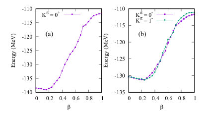
Figure 1: $K$-projected energy curves of ${}^{20}\textrm{O}$ obtained by K-VAP of $\beta$-constraint AMD plotted as a function of quadrupole deformation $\beta$. The energy curve for the $K0^{+}(\beta)$ bases is shown in panel (a) and those for the $K0^{-}(\beta)$ and $K1^{-}(\beta)$ bases are shown in panel (b).

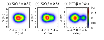
Figure 2: The matter densities of $K0^{+}$ bases at (a) $\beta=0.32$, (b) 0.52, and (c) 0.84. The intrinsic densities are integrated along the $Y$-axis and plotted on the $Z$-$X$ plane. The unit is fm^-2.

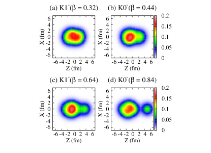
Figure 3: The same as Fig. 2 but for the (a) $K1^{-}(0.32)$, (b) $K0^{-}(0.44)$, (c) $K1^{-}(0.64)$, and (d) $K0^{-}(0.84)$ bases.

The energy spectra of ${}^{20}\textrm{O}$ are obtained after the GCM calculation using the basis wave functions obtained by K-VAP of $\beta$-constraint AMD. The calculated binding energy is $141.7$ MeV, which is slightly smaller than the experimental value ($151.36$ MeV). The positive- and negative-parity energy spectra are shown in Fig. 4 and Fig. 5, respectively. To discuss band structure, we show theoretical energy spectra for band member states, which can be classified into $K^{\pi}=0^{+}$, $K^{\pi}=0^{-}$, and $K^{\pi}=1^{-}$ bands, and that for the $1^{-}_{2}$ state along with the calculated $B(E2)$ values of in-band transitions on the left, and the experimental energy spectra and $B(E2)$ values on the right of the figures. Figures 6 and 7 show the GCM amplitudes for the band-head states, which are defined by squared overlap with each base.

Figure 4: Energy spectra of positive-parity states in ${}^{20}\textrm{O}$ obtained by GCM and those of experimental data. In the calculated spectra, the $K^{\pi}=0^{+}_{1}$, $K^{\pi}=0_{\textrm{cl,1}}^{+}$, and $K^{\pi}=0_{\textrm{cl,2}}^{+}$ bands are shown together with the $B(E2)$ values of in-band transitions. The experimental $B(E2)$ values are taken from Refs. Nakatsuka et al. (2017); Tryggestad et al. (2003). The unit of $B(E2)$ is $e^{2}$fm⁴.

Figure 5: Energy spectra of negative-parity states in ${}^{20}\textrm{O}$ obtained by GCM and experimental negative-parity spectra. In the calculated result, spectra of the $K^{\pi}=1^{-}_{1}$, $K^{\pi}=1_{\textrm{cl}}^{+}$, and $K^{\pi}=0_{\textrm{cl}}^{+}$ bands and that of the $1^{-}_{2}$ state are shown together with the $B(E2)$ ($e^{2}$fm⁴) values of in-band transitions. For the $K^{\pi}=1_{\textrm{cl}}^{+}$ band, spectra on a large scale are inserted in the figure.

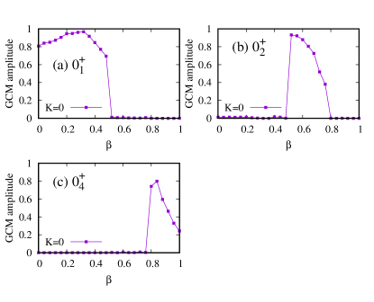
Figure 6: GCM amplitudes of the positive-parity states. The amplitudes calculated by squared overlap with the $K0^{+}(\beta)$ bases are plotted as a function of $\beta$. The results for the band-head $0_{1}^{+}$, $0_{2}^{+}$, and $0_{4}^{+}$ states of the $K^{\pi}=0^{+}_{1}$, $K^{\pi}=0^{+}_{\textrm{cl,1}}$, $K^{\pi}=0^{+}_{\textrm{cl,2}}$ bands are shown in panels (a), (b), and (c), respectively.

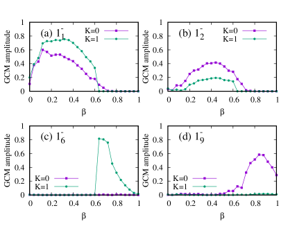
Figure 7: GCM amplitudes of the negative-parity states. The amplitudes calculated by squared overlap with the $K0^{-}(\beta)$ and $K1^{-}(\beta)$ bases are plotted by squares and circles, respectively. Panels (a), (c), and (d) show the results for the band-head $1_{1}^{-}$, $1_{6}^{-}$, and $1^{-}_{9}$ states of the $K^{\pi}=1^{-}_{1}$, $K^{\pi}=1^{-}_{\textrm{cl}}$, and $K^{\pi}=0^{-}_{\textrm{cl}}$ bands, respectively, and panel (b) shows the result for the $1_{2}^{-}$ state.

The ground band ($K^{\pi}=0^{+}_{1}$ band), which consists of the $0_{1}^{+}$, $2_{1}^{+}$, and $4_{1}^{+}$ states is constructed from the basis wave functions with weak deformation around the energy minimum of the $K^{\pi}=0^{+}$ energy curve. The calculated $E2$ transition strengths in the ground band are small because of a proton shell closure feature. This result is qualitatively consistent with the experimental $B(E2)$ value, but quantitatively, underestimates the observed data.

Above the ground band, two $K^{\pi}=0^{+}$ bands are built on the $0^{+}_{2}$ and $0^{+}_{4}$ states showing cluster structures. The lower and higher cluster bands on the $0^{+}_{2}$ and $0^{+}_{4}$ states are labeled as $K^{\pi}=0^{+}_{\textrm{cl},1}$ and $K^{\pi}=0^{+}_{\textrm{cl},2}$ bands, respectively. The former ($K^{\pi}=0^{+}_{\textrm{cl},1}$) band is mainly formed by the $K0^{+}(0.52)$ base (Fig. 2(b)), which has a deformed structure with clustering. The latter ($K^{\pi}=0^{+}_{\textrm{cl},2}$) band contains the dominant component of the $K0^{+}(0.84)$ base (Fig. 2(c)) with a developed ${}^{16}\textrm{C}+\alpha$ cluster structure. Because of the largely deformed intrinsic structure for these cluster bands, strong $E2$ transitions are obtained for in-band transitions, in particular, in the $K^{\pi}=0^{+}_{\textrm{cl},2}$ band.

In the calculated negative-parity levels, we obtain the $1^{-}_{1}$ and $1^{-}_{2}$ states in the low-energy region (see Fig. 5). The $K^{\pi}=1^{-}_{1}$ band is built on the $1^{-}_{1}$ state, whereas the $1^{-}_{2}$ state does not form a clear band structure. As shown in Fig. 7, the $1^{-}_{1}$ and $1^{-}_{2}$ states in the low-energy region contain components of basis wave functions in the $\beta\lesssim 0.6$ regions corresponding to weak or normal deformations shown in Figs. 3(a) and (b). The $1^{-}_{1}$ state is dominated by the $K1^{-}$ component, which contributes to the $K^{\pi}=1^{-}$ band structure, whereas the $1^{-}_{2}$ state contains larger $K0^{-}$ component than the $K1^{-}$ component. Note that these two states have significant $K$-mixing and shape fluctuation along $\beta$. In high-lying negative-parity spectra, $K^{\pi}=1^{-}$ and $K^{\pi}=0^{-}$ bands are formed from the $1^{-}_{6}$ and $1^{-}_{9}$ states, respectively. These bands are formed by largely deformed bases with developed cluster structures, and they can be understood as cluster bands, which we label as $K^{\pi}=1^{-}_{\textrm{cl}}$ and $K^{\pi}=0^{-}_{\textrm{cl}}$ bands, respectively. The $K^{\pi}=0^{-}_{\textrm{cl}}$ band has a remarkable cluster structure of the $K0^{-}$ bases in $\beta>0.8$ region in particular. The dominant component of this state is the $K0^{-}(0.84)$ base (Fig. 3(d)), which has a developed ${}^{16}\textrm{C}+\alpha$ structure similar to the $K^{\pi}=0^{+}_{\textrm{cl},2}$ cluster band, and therefore the $K^{\pi}=0^{+}_{\textrm{cl},2}$ and $K^{\pi}=0^{-}_{\textrm{cl}}$ are regarded as the parity partner states of the ${}^{16}\textrm{C}+\alpha$ clustering. However, the $K^{\pi}=1^{-}_{\textrm{cl}}$ band is dominated by the $K1^{-}(0.64)$ base (Fig. 3(c)) with a weaker cluster structure than the $K^{\pi}=0^{-}_{\textrm{cl}}$ band.

Although the experimental information for negative-parity states is not enough to allocate band structures, we tentatively allocate present $1^{-}_{1}$ and $1^{-}_{2}$ states to the experimental $1^{-}_{1}(5.36~{}\textrm{MeV})$ and $1^{-}_{2}(6.84~{}\textrm{MeV})$ states. The $E3$ transition from the $3^{-}\ (5.62\ \textrm{MeV})$ state to the $0^{+}_{1}$ state was observed to have a significant strength of $B(E3)=170\pm 14$ $e^{2}\textrm{fm}^{6}$ Nakatsuka et al. (2017). We obtain $B(E3;3^{-}_{1}\to 0^{+}_{1})=87.5$ $e^{2}\textrm{fm}^{6}$ between the $K^{\pi}=1^{-}_{1}$ and ground bands in this result. This value is of the same order as the experimental data and supports our conclusion that our $K^{\pi}=1^{-}_{1}$ band corresponds to the experimental $1^{-}_{1}~{}(5.36~{}\textrm{MeV})$ and $3^{-}\ (5.62\ \textrm{MeV})$ states. For dipole transition strengths from the ground to low-lying $1^{-}$ states, we will show the result in Sect. V.1 for discussions of dipole transition properties.

IV.2 Single-particle states in deformed states

To investigate single-particle configurations in a mean field picture, we analyze single-particle orbits in the dominant components of the band-head $0^{+}$ and $1^{-}$ states and the $1^{-}_{2}$ state. For each base, the wave function is expressed by a single Slater determinant, for which the nonorthogonal set of Gaussian single-particle wave functions can be transformed into an orthogonal set of single-particle orbits in a mean-field as done in Refs. Dote et al. (1997); Kanada-En’yo et al. (1999). Figures 8 and 9 show single-particle orbits in the dominant bases of the positive- and negative-parity states, respectively. For each basis, single-particle densities (color maps) of the highest neutron and proton orbits are shown together with the total proton density (contour lines).

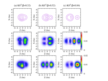
Figure 8: Density distribution of protons and those of single-particle orbits in the (a) $K0^{+}(0.32)$, (b) $K0^{+}(0.52)$, and (c) $K0^{+}(0.84)$ bases, which correspond to the $K^{\pi}=0^{+}_{1}$, $K^{\pi}=0^{+}_{\textrm{cl,1}}$, and $K^{\pi}=0^{+}_{\textrm{cl,2}}$ bands, respectively. The upper panels show the proton density distributions by the contour lines. In the middle and lower panels, the density of the highest neutron and proton orbits are shown with color maps, respectively, with the total proton density (contour lines). The matter densities of these bases are shown in Fig. 2.

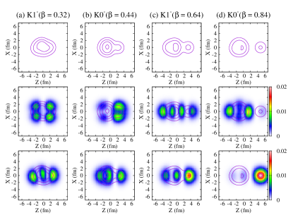
Figure 9: The same as Fig. 8, but the results for the (a) $K1^{-}(0.32)$, (b) $K0^{-}(0.44)$, (c) $K1^{-}(0.64)$, and (d) $K0^{-}(0.84)$ bases, which correspond to the $K^{\pi}=1^{-}_{1}$ band, the $1^{-}_{2}$ state, $K^{\pi}=1^{-}_{\textrm{cl}}$, and $K^{\pi}=0^{-}_{\textrm{cl}}$ bands, respectively. The matter densities of these bases are shown in Fig. 3.

Figures 8(a), (b), and (c) show results of the $K0^{+}(0.32)$, $K0^{+}(0.52)$, and $K0^{+}(0.84)$ for the $K^{\pi}=0^{+}_{1}$, $K^{\pi}=0^{+}_{\textrm{cl},1}$, and $K^{\pi}=0^{+}_{\textrm{cl},2}$ bands, respectively. The $K0^{+}(0.32)$ base for the $K^{\pi}=0^{+}_{1}$ band is described by four neutrons in $sd$-orbits around a weakly deformed core of the ${}^{16}\textrm{O}$ ground state, and it roughly corresponds to a $0\hbar\omega$ shell-model configuration. The $K0^{+}(0.52)$ base for the $K^{\pi}=0^{+}_{\textrm{cl},1}$ band has the character of two-proton excitation $p^{-2}_{\pi}(sd)^{2}_{\pi}$ of a $2\hbar\omega$ configuration in terms of the mean-field picture. In the cluster picture, the proton structure of this band has a parity asymmetric 6+2 structure and analogous to the proton part of the ${}^{16}\textrm{O}(0^{+}_{2})$ state having a ${}^{12}\textrm{C}+\alpha$ cluster structure. The $K0^{+}(0.84)$ base for the $K^{\pi}=0^{+}_{\textrm{cl},2}$ band has the developed ${}^{14}\textrm{C}+\alpha$-cluster core with two neutrons in an elongated negative-parity orbit. This neutron orbit has three nodes along the $Z$ axis and corresponds to a molecular called the $\sigma$-orbit. We label this negative-parity $\sigma$ orbit as $\sigma_{fp}$ in the association of a $fp$-orbit. The $K0^{+}(0.84)$ base is associated with $4\hbar\omega$ configuration with two-proton and neutron excitation in the mean-field picture. Note that, after the GCM calculation, the final wave function of the $K^{\pi}=0^{+}_{\textrm{cl},2}$ band contains not only the $K0^{+}(0.84)$ component but also significant mixing of $K0^{+}(\beta>0.84)$ bases with the last two neutrons not in the molecular $\sigma_{fp}$-orbit but localized around the ${}^{14}\textrm{C}$ cluster forming a dinuclear structure of ${}^{16}\textrm{C}+\alpha$ cluster. It means that the $K^{\pi}=0^{+}_{\textrm{cl},2}$ band is a mixture of two types of clustering. One is the molecular orbital structure of the ${}^{14}\textrm{C}+\alpha$ cluster core with two neutrons in the $\sigma_{fp}$-orbit and the other is the dinuclear ${}^{16}\textrm{C}+\alpha$ structure.

Figures 9 (a), (b), (c), and (d) present the results for the $K1^{-}$($0.32$), $K0^{-}$($0.44$), $K1^{-}$($0.64$), and $K0^{-}$($0.84$) bases, which correspond to the $1^{-}_{1}$ and $1^{-}_{2}$ states, and the $K^{\pi}=1^{-}_{\textrm{cl}}$ and $K^{\pi}=0^{-}_{\textrm{cl}}$ bands, respectively. The $K1^{-}$($0.32$) base for the $1^{-}_{1}$ state can be understood as one proton excitation from the $p$ shell and associated with the $(1,0,0)^{-1}(0,0,2)^{1}$ (or $(0,1,0)^{-1}(0,0,2)^{1}$) configuration in terms of harmonic oscillator orbits $(n_{x},n_{y},n_{z})$. Furthermore, the $K1^{-}$(0.44) base for the $1^{-}_{2}$ state has one proton excitation as a leading component but cannot be interpreted by a simple $1p1h$ configuration. Instead, the proton excitation induces the parity asymmetric collective excitation in the proton and neutron parts as can be seen in the asymmetry of the highest neutron orbit and that of the proton density in Fig. 9(b). The $K1^{-}(0.64)$ base for the $K^{\pi}=1^{-}_{\textrm{cl}}$ band corresponds to a $3\hbar\omega$ excitation with one neutron in the $\sigma_{fp}$-orbit around the developed cluster core having two-proton excitation. The $K0^{-}(0.84)$ base for the $K^{\pi}=0^{-}_{\textrm{cl}}$ band has the dinuclear structure of developed ${}^{16}\textrm{C}+\alpha$ clustering.

Let us compare the intrinsic configurations the positive- and negative-parity cluster bands; the $K^{\pi}=0^{+}_{\textrm{cl},1}$, $K^{\pi}=0^{+}_{\textrm{cl},2}$, $K^{\pi}=1^{-}_{\textrm{cl}}$, and $K^{\pi}=0^{-}_{\textrm{cl}}$ bands. In these four cluster bands, the proton density has asymmetric shapes due to the 6+2 structure and shows ${}^{n}\textrm{C}+\alpha$ clustering. In terms of the neutron configuration, the $K^{\pi}=0^{+}_{\textrm{cl},1}$, $K^{\pi}=1^{-}_{\textrm{cl}}$, and $K^{\pi}=0^{+}_{\textrm{cl},2}$ bands have zero, one, and two neutrons in the $\sigma_{fp}$-orbit around the cluster core, respectively. As the number of $\sigma_{fp}$-orbit neutrons increases from zero to two, the cluster structure develops. It is interesting that the $K^{\pi}=0^{+}_{\textrm{cl},2}$ band also contains significant mixing of the ${}^{16}\textrm{C}+\alpha$ component, which is the dominant component of the $K^{\pi}=0^{-}_{\textrm{cl}}$ band. Therefore, an alternative interpretation is that the $K^{\pi}=0^{+}_{\textrm{cl},2}$ and $K^{\pi}=0^{-}_{\textrm{cl}}$ bands form parity doublet partners of the ${}^{16}\textrm{C}+\alpha$ structure.

V Discussions

V.1 Properties of dipole excitations

V.1.1 Dipole transition strengths

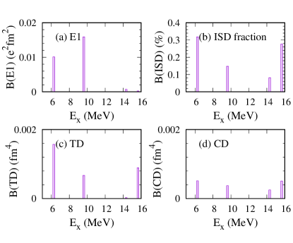
Figure 10: Dipole transition strengths for the (a) $E1$, (b) ISD, (c) TD, and (d) CD operators from the $0_{1}^{+}$ state. For the ISD operator, the energy weighted strengths are plotted in ratio to the EWSR defined by Ref. Harakeh and Dieperink (1981).

Table 1: Calculated and experimental values of the excitation energies of the $1_{1}^{-}$ and $1_{2}^{-}$ states and the $E1$ and ISD transition strengths from the $0^{+}_{1}$ state. For the ISD transitions, the energy weighted strength ratios ($f_{\textrm{ISD}}$) to the EWSR are listed. The experimental data are taken from Refs. Tryggestad et al. (2002, 2003); Nakatsuka et al. (2017).

	Calculation
	$E_{x}$ (MeV)	$B(E1)$ ($e^{2}\textrm{fm}^{2}$)	$f_{\textrm{ISD}}$ ($\%$)
$1_{1}^{-}$	6.25	$1.11\times 10^{-2}$	0.31
$1_{2}^{-}$	9.59	$1.56\times 10^{-2}$	0.15
	Experiment
	$E_{x}$ (MeV)	$B(E1)$ ($e^{2}\textrm{fm}^{2}$)	$f_{\textrm{ISD}}$ ($\%$)
$1_{1}^{-}$	5.36(5)	$3.57(20)\times 10^{-2}$	2.70(32)
$1_{2}^{-}$	6.84(7)	$3.79(26)\times 10^{-2}$	0.67(12)

The dipole transition strength function from the $0^{+}_{1}$ state is calculated using the $0^{+}_{1}$ and $1^{-}_{k}$ states obtained with the GCM calculation. Figure 10 (a) shows the $E1$ strengths. The energy-weighted ISD strengths are plotted in ratio to the EWSR as shown Fig. 10 (b). The transition strengths for the CD and TD operators are shown in Figs. 10 (c) and (d), respectively. Significant $E1$ and TD transition strengths are obtained for the two LED states, $1^{-}_{1}$ and $1^{-}_{2}$ states. The $1^{-}_{1}$ state has a remarkable TD and significant $E1$ strengths, whereas the $1_{2}^{-}$ state has remarkable $E1$ strength. Compared with the TD strengths, the CD transitions to the two LED states are rather weak as 0.3% (0.15%) of the EWSR for the $1^{-}_{1}$ ($1^{-}_{2}$) states. In Table 1, we compare the present results of the $E1$ and ISD transition strengths to the $1^{-}_{1}$ and $1^{-}_{2}$ states with the experimental data of the $1^{-}_{1}$(5.36 MeV) and $1^{-}_{2}$(6.84 MeV) states. This result qualitatively describes the significant $E1$ strengths measured for the $1^{-}_{1}$(5.36 MeV) and $1^{-}_{2}$(6.84 MeV) states, though the quantitative agreement with the data is not satisfactory. For the ISD strengths, this calculation fails to obtain significant ISD strengths as large as the observed ISD strength to the $1^{-}_{1}$ state reported recently Nakatsuka et al. (2017). Our result for weak ISD transitions to LED states agrees to a mean-field calculation Inakura and Togano (2018).

V.1.2 Transition current and strength densities for LED in ${}^{20}\textrm{O}$

We calculate the transition current and strength densities in the intrinsic frame using the dominant bases to discuss the properties of the low-energy dipole excitations $0^{+}_{1}\to 1^{-}_{1,2}$. The definitions for the transition current and strength densities are given in appendix A. For the intrinsic states of the $0^{+}_{1}$, $1^{-}_{1}$, and $1^{-}_{2}$ states, we choose the $K0^{+}(0.32)$, $K1^{-}(0.32)$, and $K0^{-}(0.44)$ bases, respectively, to describe the leading properties of each state, and calculate the transition current densities of the $K0^{+}(0.32)\to K1^{-}(0.32)$ and $K0^{+}(0.32)\to K0^{-}(0.44)$ transitions. In the calculation, normalized $K$ eigenstates projected from the wave functions $\Phi^{\pi}_{K}(\beta)$ are used as explained in appendix A. Note that, the $1^{-}_{1}$, and $1^{-}_{2}$ states significantly contain the $K$-mixing and shape fluctuation along $\beta$, which contributes to the final GCM results of the $1^{-}_{1}$, and $1^{-}_{2}$ states, but such higher order effects are omitted for simplicity in the this analysis in the intrinsic frame.

The calculated transition current densities are shown in Fig. 11. Vector plots in the left, middle, and right panels show the proton and neutron parts and the isovector component of the transition current densities, respectively. The strength densities of the TD and $E1$ operators are shown in Fig. 12. The vortical flow of the proton current density is induced by the 1 proton excitation $(1,0,0)^{-1}(0,0,2)^{1}$ in the $K0^{+}(0.32)\to K1^{-}(0.32)$ transition, which corresponds to the $1^{-}_{1}$ excitation as shown in the transition current density in Fig. 11(a). This vortical proton current contributes to the remarkable TD strength density as shown in Fig. 12(a) and describes the TD nature of the $1^{-}_{1}$ excitation. However, the $K0^{+}(0.32)\to K0^{-}(0.44)$ transition for the $1^{-}_{2}$ excitation show a translational flow along the deformed ($Z$) axis rather than a vortical flow (see Fig. 11(b)). The neutron part of the translational flow, in particular, is widely distributed across a wide $X$ range. The surface neutron flow in the region of $|X|=2$–4 fm and $Z\sim 2$ fm is produced by valence neutron oscillation in the parity asymmetric orbit (Fig. 9(b)) around the prolate core, which is induced by the proton excitation. This neutron surface flow, as shown in Fig. 12(d), gives the dominant contribution to the $E1$ strength of the $K0^{+}(0.32)\to K0^{-}(0.44)$ transition and is a major source of the strong $E1$ transition to the $1^{-}_{2}$ state. In the internal region of the prolately deformed core, the proton and neutron flows cancel each other, but give some contribution to the $E1$ strength because of the recoil effect. This result indicates that the parity asymmetry of the cluster core and that of the valence neutron orbit, which are induced by the two-proton excitation, play an important role in the enhanced $E1$ strength of the $K0^{-}(0.44)$ base.

In the this analysis of the $K1^{-}(0.32)$ and $K0^{-}(0.44)$ bases, a clear difference is found in the transition properties between the two LED modes; the TD nature in the $K1^{-}(0.32)$ base and the $E1$ character in the $K0^{-}(0.44)$ base. These two LED modes, the TD and $E1$ modes appear separately as vortical and translational excitations of nuclear current in the $K^{\pi}=1^{-}$ and $K^{\pi}=0^{-}$ components of the deformed states, respectively. However they couple with each other in the $1^{-}_{1}$ and $1^{-}_{2}$ states after the superposition of the GCM calculation via significant $K$-mixing and shape fluctuation as mentioned previously. Therefore, the TD strength of the $K1^{-}(0.32)$ base is fragmented into the $1^{-}_{1}$ and $1^{-}_{2}$ states, and the $E1$ strength of the $K0^{-}(0.44)$ base is split into the two states. Nevertheless, since the $1^{-}_{1}$ state retains the dominant TD nature, it has a relatively large TD strength and constructs the $K^{\pi}=1^{-}$ band structure.

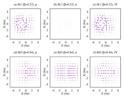
Figure 11: (upper) Transition current densities $\delta\mbox{\boldmath$j$}^{K}(\mbox{\boldmath$r$})$ from the $K0^{+}(0.32)$ base to the $K1^{-}(0.32)$ corresponding to the $0^{+}_{1}\to 1^{-}_{1}$ transition and (lower) those to the $K0^{-}(0.44)$ base for $0^{+}_{1}\to 1^{-}_{2}$. The vector plots of the densities in the $Z$-$X$ plane at $Y=0$ are shown. The proton and neutron currents are shown in the left and middle, respectively, and the isovector currents are shown in the right. The vector plots are multiplied by 30 in (a)-(c), by 50 in (d) and (e), and by 100 in panel (f).

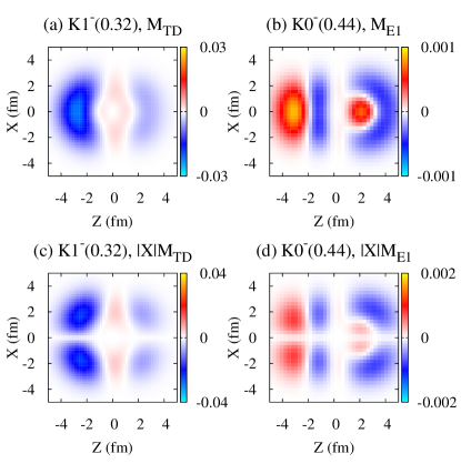
Figure 12: (Left) TD strength densities ${\cal M}^{K}_{\textrm{TD}}$ for $K0^{+}(0.32)\to K1^{-}(0.32)$ and (Right) $E1$ strength densities ${\cal M}^{K}_{E1}$ for $K0^{+}(0.32)\to K0^{-}(0.44)$. The former and the latter correspond to the $0^{+}_{1}\to 1^{-}_{1}$ and $0^{+}_{1}\to 1^{-}_{2}$ transitions, respectively. The strength densities ${\cal M}^{K}(X,Y,Z)$ and $|X|$-weighted values $|X|{\cal M}^{K}(X,Y,Z)$ on the $Z$-$X$ plane at $Y=0$ are shown in upper and lower panels, respectively.

V.2 Systematic analysis of LED excitations in O isotopes

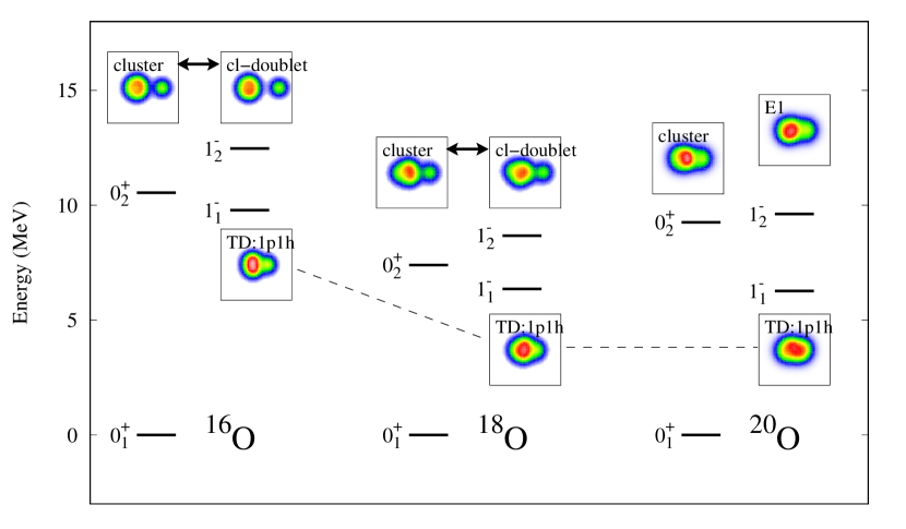
Figure 13: Energy spectra of the $0^{+}_{1,2}$ and $1^{-}_{1,2}$ states in ${}^{16}\textrm{O}$, ${}^{18}\textrm{O}$, and ${}^{20}\textrm{O}$ calculated with K-VAP and GCM of $\beta$-constraint AMD. For excited states, intrinsic matter densities of the dominant bases are also shown with labels “TD:1p1h”, “cluster”, “cluster-doublet”, and “E1”, which indicate the TD mode with $1p$-$1h$ configuration, $K^{\pi}=0^{+}$ cluster state, its parity doublet $K^{\pi}=0^{-}$ state, and the $E1$ mode, respectively. The color map plotting of densities is the same as Fig. 2.

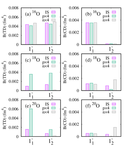
Figure 14: The IS, proton, and neutron components of the TD and CD strengths for the $1^{-}_{1}$ and $1^{-}_{2}$ states of ${}^{16}\textrm{O}$, ${}^{18}\textrm{O}$, and ${}^{20}\textrm{O}$ calculated with K-VAP and GCM of $\beta$-constraint AMD. The TD strengths of (a) ${}^{16}\textrm{O}$, (c) ${}^{18}\textrm{O}$, and (e) ${}^{20}\textrm{O}$ are shown in the left, and the CD strengths of (b) ${}^{16}\textrm{O}$, (d) ${}^{18}\textrm{O}$, and (f) ${}^{20}\textrm{O}$ are shown in the right. Proton and neutron components are multiplied by a factor of four to compare the IS component. The results for ${}^{16}\textrm{O}$ and ${}^{18}\textrm{O}$ are taken from Refs. Shikata and Kanada-En’yo (2020, 2021).

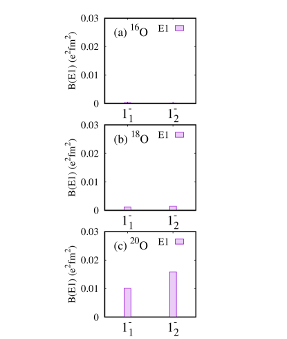
Figure 15: $E1$ strengths for the $1^{-}_{1}$ and $1^{-}_{2}$ states of (a)${}^{16}\textrm{O}$, (b)${}^{18}\textrm{O}$, and (c)${}^{20}\textrm{O}$ calculated with K-VAP and GCM of $\beta$-constraint AMD. The results for ${}^{18}\textrm{O}$ are taken from Ref. Shikata and Kanada-En’yo (2021).

To clarify the roles of valence neutrons in the LED excitations in ${}^{20}\textrm{O}$, we discuss systematics of dipole excitation properties in O isotopes by comparing the present results with previous results obtained using the same framework for ${}^{16}\textrm{O}$ and ${}^{18}\textrm{O}$. Figure 13 shows the theoretical energy spectra of the $0^{+}_{1,2}$ and $1^{-}_{1,2}$ states in ${}^{16}\textrm{O}$, ${}^{18}\textrm{O}$, and ${}^{20}\textrm{O}$. The intrinsic matter densities of the dominant bases in the excited states are also shown in the figure. In each of ${}^{16}\textrm{O}$, ${}^{18}\textrm{O}$, and ${}^{20}\textrm{O}$, two $1^{-}$ states are obtained in the low-energy region.

These LED states have significant isoscalar dipole strengths of the TD and/or CD operators. Figure  14 shows the isoscalar, proton, and neutron components of the TD and CD strengths for the $1^{-}_{1}$ and $1^{-}_{2}$ states of the O isotopes. According to the previous analysis, we identified the ${}^{16}\textrm{O}(1^{-}_{1})$ and ${}^{18}\textrm{O}(1^{-}_{1})$ states as TD mode, which is characterized by the vortical flow of the transition current densities. These LED states in ${}^{16}\textrm{O}$ and ${}^{18}\textrm{O}$ correspond to the present TD mode of the ${}^{20}\textrm{O}(1^{-}_{1})$ state. The TD mode is described by the $K^{\pi}=1^{-}$ component of the $1p$-$1h$ excitation of deformed states in all three cases. The isoscalar components of the TD strengths of the $1^{-}_{1}$ and $1^{-}_{2}$ states are largest in ${}^{16}\textrm{O}$ because of the coherent (isoscalar) contribution from the proton and neutron parts, but relatively small in ${}^{18}\textrm{O}$ and ${}^{20}\textrm{O}$ because of the lack of contribution from the neutron part.

Figure 15 shows the $E1$ strengths for the $1^{-}_{1}$ and $1^{-}_{2}$ states of the O isotopes. The low-energy $E1$ mode is obtained only in the ${}^{20}\textrm{O}$ as the ${}^{20}\textrm{O}(1^{-}_{2})$ state, which is produced by the previously described surface neutron oscillation on the prolate deformation induced by proton excitation. The ${}^{16}\textrm{O}(1^{-}_{2})$ and ${}^{18}\textrm{O}(1^{-}_{2})$ states are not $E1$ modes but have a distinct character, that is, the asymmetric cluster structure that forms parity partners with the ${}^{16}\textrm{O}(0^{+}_{2})$ and ${}^{18}\textrm{O}(0^{+}_{2})$ states, respectively. Note that the ${}^{20}\textrm{O}(0^{+}_{2})$ state has a cluster structure but its parity doublet partner $1^{-}$ state is not obtained. In the structure change from the ${}^{16}\textrm{O}(0^{+}_{2})$ state along the isotope chain, the clustering is weakened in the ${}^{18}\textrm{O}(0^{+}_{2})$ state and further suppressed in the ${}^{20}\textrm{O}(0^{+}_{2})$ state by excess neutrons and no longer constructs the parity doublet $1^{-}$ state of the ${}^{20}\textrm{O}(0^{+}_{2})$ state.

Finally, we comment on the CD strengths in the LED states of O isotopes. As shown in Fig. 14(a), the strong CD transition was obtained in the TD mode of ${}^{16}\textrm{O}$, which is consistent with the experimental observation of the ISD strength of the ${}^{16}\textrm{O}(1^{-}_{1})$. However, the present calculation does not degenerate such a strong CD strength in the TD mode of ${}^{20}\textrm{O}$, and fails to describe the observed ISD strength of the ${}^{20}\textrm{O}(1^{-}_{1})$ state. According to the previous analysis in Ref. Shikata and Kanada-En’yo (2020), the origin of the strong CD transition in the ${}^{16}\textrm{O}(1^{-}_{1})$ state is significant $K$-mixing of the TD mode and coupling with other deformed bases via the $\beta$ fluctuation. The contribution of the CD strengths contained in the $K0^{-}$ component of the normal deformation is essential. However, in the present result of ${}^{20}\textrm{O}$, the low-lying $E1$ appears in the $K0^{-}$ component of the normal deformation, which contributes only weakly to the CD strength. In the present calculation of GCM along the $\beta$ deformation, only the lowest base at each $\beta$ is obtained by the energy optimization, and thus energetically higher bases containing the CD strength may be missing. To overcome this problem, it is necessary to extend the present framework to properly include important bases for the low-lying CD strengths.

VI Summary

K-VAP and GCM of $\beta$-constraint AMD were used to investigate LED excitations in ${}^{20}\textrm{O}$. Two LED states, the $1^{-}_{1}$ and $1^{-}_{2}$ states were obtained. The $1^{-}_{1}$ state is a weakly deformed state with one-proton excitation, whereas the $1^{-}_{2}$ state has a normal deformation with the parity asymmetric structure.

In a detailed analysis of the dipole transition properties of these LED states, the $1^{-}_{1}$ state is considered the TD mode, while the $1^{-}_{2}$ state is associated with a low-energy $E1$ mode. The TD strength in the former mode is produced by vortical nuclear current, whereas the $E1$ strength in the latter mode is contributed by surface neutron current on the prolate deformation induced by proton excitation. These two modes, the TD (vortical) and $E1$ modes, appear separately as the $K^{\pi}=1^{-}$ and $K^{\pi}=0^{-}$ components of the deformed states, but they couple with each other in the $1_{1}^{-}$ and $1_{2}^{-}$ states of ${}^{20}\textrm{O}$ via the $K$-mixing and shape fluctuation along $\beta$. Therefore, the TD and $E1$ strengths are fragmented into both $1^{-}$ states.

In comparison with the experimental data of the $E1$ and ISD transition strengths to the $1^{-}_{1}$(5.36 MeV) and the $1^{-}_{2}$(6.84 MeV) states, the present calculation qualitatively described the experimental $E1$ strengths for the $1^{-}_{1}$ and $1^{-}_{2}$ states, but much underestimated the significant ISD transition strengths observed for the $1^{-}_{1}$ state by one order.

To clarify the roles of valence neutrons in LED excitations in ${}^{20}\textrm{O}$, systematics of the LED excitations in ${}^{16}\textrm{O}$, ${}^{18}\textrm{O}$, and ${}^{20}\textrm{O}$ were discussed in comparison for the present ${}^{20}\textrm{O}$ result with the previous ${}^{16}\textrm{O}$ and ${}^{18}\textrm{O}$ results obtained using the same framework. The TD mode was obtained as the lowest $1^{-}_{1}$ state in ${}^{16}\textrm{O}$, ${}^{18}\textrm{O}$, and ${}^{20}\textrm{O}$. However, the low-energy $E1$ mode was found only in the ${}^{20}\textrm{O}(1^{-}_{2})$ state but not in the ${}^{16}\textrm{O}$ and ${}^{18}\textrm{O}$ systems. Instead, the previous results indicated that the ${}^{16}\textrm{O}(1^{-}_{2})$ and ${}^{18}\textrm{O}(1^{-}_{2})$ states differ from the ${}^{20}\textrm{O}(1^{-}_{2})$ state and are parity doublet partners in the $K^{\pi}=0^{-}$ cluster band with the $0^{+}_{2}$ states in the $K^{\pi}=0^{+}$ bands.

Appendix A Densities of intrinsic system in the body-fixed frame

Isoscalar and isovector components of the density and current density operators are defined as,

$$\rho(\mbox{\boldmath$r$})=\sum_{k=1}^{A}\delta(\mbox{\boldmath$r$}-\mbox{\boldmath$r$}_{k}),$$ (13)

$$\rho_{\textrm{IV}}=\sum_{k=1}^{A}\frac{e^{\textrm{eff}}}{e}\delta(\mbox{\boldmath$r$}-\mbox{\boldmath$r$}_{k}),$$ (14)

$$\mbox{\boldmath$j$}_{\textrm{nucl}}(\mbox{\boldmath$r$})=\frac{-i\hbar}{2m}$$

$$\quad\times\sum_{k=1}^{A}\{\mbox{\boldmath$\nabla$}_{k}\delta(\mbox{\boldmath$r$}-\mbox{\boldmath$r$}_{k})+\delta(\mbox{\boldmath$r$}-\mbox{\boldmath$r$}_{k})\mbox{\boldmath$\nabla$}_{k}\},$$ (15)

$$\mbox{\boldmath$j$}_{\textrm{nucl},\textrm{IV}}(\mbox{\boldmath$r$})=\frac{-i\hbar}{2m}$$

$$\quad\times\sum_{k=1}^{A}\frac{e^{\textrm{eff}}}{e}\{\mbox{\boldmath$\nabla$}_{k}\delta(\mbox{\boldmath$r$}-\mbox{\boldmath$r$}_{k})+\delta(\mbox{\boldmath$r$}-\mbox{\boldmath$r$}_{k})\mbox{\boldmath$\nabla$}_{k}\},$$ (16)

where the factor $e^{\textrm{eff}}/e$ is $N/A$ for protons and $-Z/A$ for neutrons. The diagonal densities for $|k\rangle=|\Phi^{\pi}_{K}(\beta)\rangle$ are expressed as,

$$\rho(\mbox{\boldmath$r$}) \equiv \langle k|\hat{\rho}(\mbox{\boldmath$r$})|k\rangle,$$ (17)

$$\rho_{\textrm{IV}}(\mbox{\boldmath$r$}) \equiv \langle k|\hat{\rho}_{\textrm{IV}}(\mbox{\boldmath$r$})|k\rangle.$$ (18)

The transition densities and transition current densities for initial $|i\rangle$ and final $|f\rangle$ states are given as,

$$\delta\rho(\mbox{\boldmath$r$}) \equiv \langle f|{\hat{\rho}}(\mbox{\boldmath$r$})|i\rangle,$$ (19)

$$\delta\rho_{\textrm{IV}}(\mbox{\boldmath$r$}) \equiv \langle f|{\hat{\rho}}_{\textrm{IV}}(\mbox{\boldmath$r$})|i\rangle,$$ (20)

$$\delta\mbox{\boldmath$j$}(\mbox{\boldmath$r$}) \equiv \langle f|\hat{\mbox{\boldmath$j$}}_{\textrm{nucl}}(\mbox{\boldmath$r$})|i\rangle,$$ (21)

$$\delta\mbox{\boldmath$j$}_{\textrm{IV}}(\mbox{\boldmath$r$}) \equiv \langle f|\hat{\mbox{\boldmath$j$}}_{\textrm{nucl,IV}}(\mbox{\boldmath$r$})|i\rangle.$$ (22)

In the present calculation with K-VAP of $\beta$-constraint AMD, each intrinsic wave function $\Phi^{\pi}_{K}(\beta)$ for a $K0^{+}(\beta)$, $K0^{-}(\beta)$, or $K1^{-}(\beta)$ base is expressed by a Slater determinant, and its intrinsic densities are given as the diagonal densities calculated for $|k\rangle=|\Phi^{\pi}_{K}(\beta)\rangle$. The transition densities and transition current densities from a $K0^{+}(\beta_{0})$ base to $K1^{-}(\beta_{1})$ and $K0^{-}(\beta_{2})$ bases are calculated in the intrinsic (body-fixed) frame for the $K$-projected bases,

$$|i\rangle=\hat{P}^{K=0}|\Phi^{+}_{K=0}(\beta_{0})\rangle,$$ (23)

$$|f\rangle=\frac{\hat{P}^{K=-1}-\hat{P}^{K=1}}{\sqrt{2}}|\Phi^{-}_{K=1}(\beta_{1})\rangle\equiv|f^{K=1}\rangle,$$ (24)

$$|f\rangle=\hat{P}^{K=0}|\Phi^{-}_{K=0}(\beta_{2})\rangle\equiv|f^{K=0}\rangle,$$ (25)

where $|i\rangle$ and $|f\rangle$ are normalized as $\langle i|i\rangle=\langle f|f\rangle=1$ by definition. The local matrix elements ${\cal M}_{\textrm{TD,}E1}^{K}(\mbox{\boldmath$r$})$ of the TD and $E1$ operators are calculated at $Y=0$ on the $Z$-$X$ plane in the intrinsic frame as,

$$\mathcal{M}_{\textrm{TD}}^{K=0}(X,0,Z)=\frac{1}{10c}\sqrt{\frac{3}{4\pi}}$$

$$\qquad\times\left[(2X^{2}+Z^{2})\delta j^{K=0}_{Z}-ZX\delta j^{K=0}_{X}\right],$$ (26)

$$\mathcal{M}_{\textrm{TD}}^{K=1}(X,0,Z)=\frac{1}{10c}\sqrt{\frac{3}{4\pi}}$$

$$\qquad\times\left[(X^{2}+2Z^{2})\delta j^{K=1}_{X}-ZX\delta j^{K=1}_{Z}\right],$$ (27)

$$\mathcal{M}_{E1}^{K=0}(X,0,Z)=\sqrt{\frac{3}{4\pi}}Z\delta\rho^{K=0}_{\textrm{IV}},$$ (28)

$$\mathcal{M}_{E1}^{K=1}(X,0,Z)=\sqrt{\frac{3}{8\pi}}X\delta\rho^{K=1}_{\textrm{IV}},$$ (29)

where $\delta\rho^{K}_{\textrm{IV}}=\langle f^{K}|{\hat{\rho}}_{\textrm{IV}}(\mbox{\boldmath$r$})|i\rangle$ and $\delta\mbox{\boldmath$j$}^{K}=\langle f^{K}|\hat{\mbox{\boldmath$j$}}_{\textrm{nucl}}(\mbox{\boldmath$r$})|i\rangle$ at $\mbox{\boldmath$r$}=(X,0,Z)$. Note that $\mathcal{M}_{\textrm{TD}}^{K}(\mbox{\boldmath$r$})$ and $\mathcal{M}_{E1}^{K}(\mbox{\boldmath$r$})$ correspond to the integrand of the TD and $E1$ transition matrix elements and are termed TD and $E1$ strength densities, respectively, in this paper.

References

- Paar et al. (2007) N. Paar, D. Vretenar, E. Khan, and G. Colo, Rept. Prog. Phys. 70, 691 (2007).
- Aumann and Nakamura (2013) T. Aumann and T. Nakamura, Phys Scr 2013, 014012 (2013).
- Savran et al. (2013) D. Savran, T. Aumann, and A. Zilges, Prog. Part. Nucl. Phys. 70, 210 (2013).
- Bracco et al. (2015) A. Bracco, F. Crespi, and E. Lanza, Eur. Phys. J. A 51, 99 (2015).
- Harakeh and Dieperink (1981) M. N. Harakeh and A. E. L. Dieperink, Phys. Rev. C 23, 2329 (1981).
- Decowski et al. (1981) P. Decowski, H. P. Morsch, and W. Benenson, Phys. Lett. B 101, 147 (1981).
- Poelhekken et al. (1992) T. D. Poelhekken et al., Phys. Lett. B 278, 423 (1992).
- John et al. (2003) B. John et al., Phys. Rev. C 68, 014305 (2003).
- Tryggestad et al. (2002) E. Tryggestad et al., Phys. Lett. B 541, 52 (2002).
- Tryggestad et al. (2003) E. Tryggestad et al., Phys. Rev. C 67, 064309 (2003).
- Nakatsuka et al. (2017) N. Nakatsuka et al., Phys. Lett. B 768, 387 (2017).
- Gibelin et al. (2008) J. Gibelin et al., Phys. Rev. Lett. 101, 212503 (2008).
- Hartmann et al. (2000) T. Hartmann, J. Enders, P. Mohr, K. Vogt, S. Volz, and A. Zilges, Phys. Rev. Lett. 85, 274 (2000).
- Derya et al. (2014) V. Derya et al., Phys. Lett. B 730, 288 (2014).
- Brzosko et al. (1969) J. S. Brzosko, E. Gierlik, A. Soltan Jr., and Z. Wilhelmi, Can. J. Phys. 47, 2849 (1969).
- Ikeda (1988) K. Ikeda, INS Report JHP-7 (in Japan) (1988).
- Semenko (1981) S. F. Semenko, Sov. J. Nucl. Phys. 34, 356 (1981).
- Ravenhall and Wambach (1987) D. G. Ravenhall and J. Wambach, Nucl. Phys. A 475, 468 (1987).
- Ryezayeva et al. (2002) N. Ryezayeva et al., Phys. Rev. Lett. 89, 272502 (2002).
- Papakonstantinou et al. (2011) P. Papakonstantinou, V. Y. Ponomarev, R. Roth, and J. Wambach, Eur. Phys. J. A 47, 14 (2011), arXiv:1011.1162 [nucl-th] .
- Kvasil et al. (2011) J. Kvasil et al., Phys. Rev. C 84, 034303 (2011).
- Repko et al. (2013) A. Repko, P. G. Reinhard, V. O. Nesterenko, and J. Kvasil, Phys. Rev. C 87, 024305 (2013).
- Kvasil et al. (2014) J. Kvasil, V. O. Nesterenko, W. Kleinig, and P. G. Reinhard, Phys Scr 89, 054023 (2014).
- Nesterenko et al. (2016) V. O. Nesterenko et al., Phys. Atom. Nucl. 79, 842 (2016).
- Nesterenko et al. (2018) V. O. Nesterenko, A. Repko, J. Kvasil, and P. G. Reinhard, Phys. Rev. Lett. 120, 182501 (2018).
- Chiba et al. (2016) Y. Chiba, M. Kimura, and Y. Taniguchi, Phys. Rev. C 93, 034319 (2016).
- Kanada-En’yo and Shikata (2017) Y. Kanada-En’yo and Y. Shikata, Phys. Rev. C 95, 064319 (2017).
- Kanada-En’yo et al. (2018) Y. Kanada-En’yo, Y. Shikata, and H. Morita, Phys. Rev. C 97, 014303 (2018).
- Kanada-En’yo and Shikata (2019) Y. Kanada-En’yo and Y. Shikata, Phys. Rev. C 100, 014301 (2019), 1903.01075 [nucl-th] .
- Shikata et al. (2019) Y. Shikata, Y. Kanada-En’yo, and H. Morita, Prog. Theor. Exp. Phys. 2019, 063D01 (2019).
- Shikata and Kanada-En’yo (2020) Y. Shikata and Y. Kanada-En’yo, Prog. Theor. Exp. Phys. 2020, 073D01 (2020).
- Shikata and Kanada-En’yo (2021) Y. Shikata and Y. Kanada-En’yo, Phys. Rev. C 103, 034312 (2021), arXiv:2011.00821 [nucl-th] .
- Sagawa and Suzuki (1999) H. Sagawa and T. Suzuki, Phys. Rev. C 59, 3116 (1999).
- Colo and Bortignon (2001) G. Colo and P. F. Bortignon, Nucl. Phys. A 696, 427 (2001).
- Sagawa and Suzuki (2001) H. Sagawa and T. Suzuki, Nucl. Phys. A 687, 111 (2001).
- Vretenar et al. (2001) D. Vretenar, N. Paar, P. Ring, and G. A. Lalazissis, Nucl. Phys. A 692, 496 (2001).
- Paar et al. (2003) N. Paar, P. Ring, T. Niksic, and D. Vretenar, Phys. Rev. C 67, 034312 (2003).
- Inakura and Togano (2018) T. Inakura and Y. Togano, Phys. Rev. C 97, 054330 (2018).
- Gai et al. (1983) M. Gai et al., Phys. Rev. Lett. 50, 239 (1983).
- Gai et al. (1987) M. Gai, R. Keddy, D. Bromley, J. Olness, and E. Warburton, Phys. Rev. C 36, 1256 (1987).
- Gai et al. (1991) M. Gai, M. Ruscev, D. Bromley, and J. Olness, Phys. Rev. C 43, 2127 (1991).
- Furutachi et al. (2008) N. Furutachi et al., Prog. Theor. Phys. 119, 403 (2008).
- Baba and Kimura (2019) T. Baba and M. Kimura, Phys. Rev. C 100, 064311 (2019).
- Baba and Kimura (2020) T. Baba and M. Kimura, Phys. Rev. C 102, 024317 (2020).
- Leistenschneider et al. (2001) A. Leistenschneider et al., Phys. Rev. Lett. 86, 5442 (2001).
- (46) Y. Kanada-Enyo, H. Horiuchi, and A. Ono, .
- Kimura et al. (2001) M. Kimura, Y. Sugawa, and H. Horiuchi, Prog. Theor. Phys. 106, 1153 (2001).
- Kanada-En’yo and Horiuchi (2001) Y. Kanada-En’yo and H. Horiuchi, Prog. Theor. Phys. Suppl. 142, 205 (2001).
- (49) Y. Kanada-En’yo, M. Kimura, and A. Ono, arXiv:1202.1864 [nucl-th] .
- Kimura et al. (2016) M. Kimura, T. Suhara, and Y. Kanada-En’yo, Eur. Phys. J. A 52, 373 (2016).
- Kanada-En’yo (1998) Y. Kanada-En’yo, Phys. Rev. Lett. 81, 5291 (1998).
- Suhara and Kanada-En’yo (2010) T. Suhara and Y. Kanada-En’yo, Prog. Theor. Phys. 123, 303 (2010).
- Kvasil et al. (2003) J. Kvasil, N. L. Iudice, C. Stoyanov, and P. Alexa, J. Phys. G: Nucl. Part. Phys. 29, 753 (2003).
- Ando et al. (1980) T. Ando, K. Ikeda, and A. Tohsaki-Suzuki, Prog. Theor. Phys. 64, 1608 (1980).
- Tamagaki (1968) R. Tamagaki, Prog. Theor. Phys. 39, 91 (1968).
- Yamaguchi et al. (1979) N. Yamaguchi, T. Kasahara, S. Nagata, and Y. Akaishi, Prog. Theor. Phys. 62, 1018 (1979).
- Kanada-En’yo et al. (1999) Y. Kanada-En’yo, H. Horiuchi, and A. Dote, Phys. Rev. C 60, 064304 (1999).
- Kanada-En’yo (2007) Y. Kanada-En’yo, Prog. Theor. Phys. 117, 655 (2007).
- Kanada-En’yo (2017) Y. Kanada-En’yo, Phys. Rev. C 96, 034306 (2017).
- Kanada-En’yo and Ogata (2020) Y. Kanada-En’yo and K. Ogata, Phys. Rev. C 101, 064308 (2020).
- Dote et al. (1997) A. Dote, H. Horiuchi, and Y. Kanada-En’yo, Phys. Rev. C 56, 1844 (1997).