Description of an ecological niche
for a mixed local/nonlocal dispersal:
an evolution equation and a new Neumann condition arising from the superposition
of Brownian and Lévy processes

Abstract.

We propose here a motivation for a mixed local/nonlocal problem with a new type of Neumann condition.

Our description is based on formal expansions and approximations. In a nutshell, a biological species is supposed to diffuse either by a random walk or by a jump process, according to prescribed probabilities. If the process makes an individual exit the niche, it must come to the niche right away, by selecting the return point according to the underlying stochastic process. More precisely, if the random particle exits the domain, it is forced to immediately reenter the domain, and the new point in the domain is chosen randomly by following a bouncing process with the same distribution as the original one.

By a suitable definition outside the niche, the density of the population ends up solving a mixed local/nonlocal equation, in which the dispersion is given by the superposition of the classical and the fractional Laplacian. This density function satisfies two types of Neumann conditions, namely the classical Neumann condition on the boundary of the niche, and a nonlocal Neumann condition in the exterior of the niche.

1. Introduction

The goal of this note is to provide an intuitive mathematical explanation related to a recent model proposed in [VERO] to describe the diffusion of a biological population living in an ecological niche and subject to both local and nonlocal dispersals. The model is motivated by the biologically relevant situation of a population following long-jump foraging patterns alternated with focused searching strategies at small scales. The exterior of the niche is accessible by the population, but presents a hostile environment that forces the population to an immediate return to the niche after a possible egression.

Namely, we present a model of an evolution equation driven by a diffusive operator of mixed local and nonlocal type (that is, the sum of a classical and a fractional Laplacians) with a perspective proper for application in ecology. The solution of this evolution equation represents the density of a biological population living in an ecological niche, which in turn corresponds to the domain in which the equation takes place. The mixed operator is the outcome of a superposition of a classical (i.e. Brownian) and a long-range (i.e. Lévy) stochastic processes. In particular, we are interested in describing the situation in which the population exits the biological niche and immediately comes back to it by following the above mentioned stochastic process: this phenomenon naturally leads to the study of a new type of mixed Neumann condition made of two separate prescriptions (namely, a classical Neumann condition on the boundary of the given domain and a nonlocal Neumann condition set on the exterior of the domain).

More specifically, the main mathematical framework presented in [VERO] can be described by the diffusive equation (endowed with external data)

$$\begin{split}&\frac{\partial U}{\partial t}=\alpha\Delta U-\beta(-\Delta)^{s}U\qquad{\mbox{ in }}\;\Omega\times(0,+\infty),\\ &{\mbox{where }}\qquad(-\Delta)^{s}U(x):=\int_{\mathbb{R}^{n}}\frac{U(x)-U(y)}{|x-y|^{n+2s}}\,dy,\end{split}$$ (1.1)

$$\lim_{\vartheta\to 0^{+}}\frac{U(x+\vartheta\nu,t)-U(x,t)}{\vartheta}=:\frac{\partial U}{\partial\nu}(x)=0\qquad{\mbox{ for every }}\;x\in\partial\Omega,$$ (1.2)

$$\int_{\Omega}\frac{U(x)-U(y)}{|x-y|^{n+2s}}\,dy=0\qquad{\mbox{ for every }}\;x\in\mathbb{R}^{n}\setminus\overline{\Omega}.$$ (1.3)

In this setting, $U=U(x,t)$ is a smooth function depending on the space variables $x\in\mathbb{R}^{n}$ and $t\in[0,+\infty)$, possibly endowed with some initial condition at time $t=0$. The diffusive parameters $\alpha$ and $\beta$ are positive constants, $\Omega$ is a, say, bounded and smooth domain in $\mathbb{R}^{n}$, with external unit normal given by $\nu$, and $s\in(0,1)$. Also, the integral in (1.1) is evaluated in the principal value sense whenever needed to cope with the singularity produced by the vanishing of the denominator.

The biological interpretation of the setting in (1.1)–(1.3) arises from a biological population with density $u=u(x,t)$ living in the niche described by the domain $\Omega$: then, the function $U$ in (1.1)–(1.3) is obtained from $u$ in such a way that $U$ coincides with $u$ in $\Omega$ and it is a convenient extension of $u$ outside $\Omega$. Hence, the knowledge of the function $U$ in (1.1)–(1.3) completely determines the density of the biological population in the niche (in addition, as pointed out in [MR4102340] the setting in (1.1)–(1.3) for $U$ can be reformulated as a regional problem in $\Omega$ for an integrodifferential operator for $u$ whose kernel has a logarithmic singularity along $\partial\Omega$, see also [AUD]).

The population diffuses according to two types of dispersals, namely a classical one, related to the classical Laplacian, and a nonlocal one, modeled on Lévy flights and encoded by the fractional Laplacian in (1.1). While the occurrence of nonlocal diffusion in biological species is an extensively studied phenomenon (see e.g. [NATU, NATU2]) and it is commonly known that captivity is lethal for some species used to cruise broad open distances at a time (see e.g. [POL, POL2, SHARK] – suggesting that for such species the classical Neumann condition is somehow as lethal as a homogeneous Dirichlet condition), a precise description on how this is compatible with the existence of a prescribed niche for the population is a topic of current investigation, and the contribution in [VERO] was precisely to propose a clear mathematical framework to settle a model in which both classical and anomalous diffusions take place, the case of purely nonlocal diffusion being firstly introduced in [dirova]. To make the model biologically richer, in [VERO] the dispersal operator was also complemented by a logistic equation taking into account the competition for resources and also by an auxiliary possible pollination (or mating call) term allowing a rise of the birth rate in view of some interactions between individuals located at some range from each other.

The importance of methods from probability and statistics to address the question of animal foraging also emerged in the analysis of the best strategy for the search of randomly located targets, see [89897765NATU, VISWANATHAN2001, MR2609393, MR3403266]. With respect to this, we recall that the foraging efficiency problem presents multifaceted features, depending, for instance, on whether the target is stationary or in motion (and with which velocity with respect to the forager), on whether or not the forager is capable of spotting the target at a finite distance or sense targets while moving, on whether or not the forager eliminates the targets when it finds them. The answer to the optimal foraging strategy is very sensible to all these details, as well as to the density of the targets and, of course, to the notion of optimality and foraging efficiency chosen to quantify and compare the different possible strategies: a possible paradigm emerging to different analyses seems to be that Lévy processes provide optimal search strategies in case of sparse, randomly distributed, immobile, revisitable targets in unbounded domains, since a long-jump searching strategy avoids oversampling (or at least allows to sample regions more quickly) in these situations, and in several destructive situations (when the forager eliminates the target) the “ballistic” limit (corresponding to the case $s\to 0^{+}$ in our notation) happens to offer the highest foraging performances – conversely, Brownian strategies outperform Lévy ones in case of densely distributed targets, see e.g. [KlagesR] for a thorough review of different possible scenarios.

As a general remark, we recall that the biological paradigm relating Lévy flights to the search strategies of biological organisms is still under intense debate and the applicability of simple, attractive and “universal” mathematical formulations has sometimes to face complex situations in which the details of the biological setting under consideration may turn the problem around and require new observations, ideas and methodologies. As a matter of fact, the possible source of errors in the biological data is certainly multifarious. Besides the difficulty of testing extensively a sufficiently large number of individuals, possibly following precisely all their movements in order to obtain data with a solid statistical significance, the environment in which the experiment is set may also offer, by its own nature, unexpected pitfalls for the collection of reliable results. A prototypical example of this difficulty is embodied by the case of wandering albatrosses who dive into the water to catch food, which, for more than a decade, in view of [NATU], were considered as the most prominent example of forager performing Lévy flight: in this pioneering experiment, sensors were attached to the feet of the birds and the duration of a flight was measured by the interval of time for which the sensor remained dry. In addition to the limited amount of data (five albatrosses engaged in 19 foraging bouts), as outlined in [NATUBIS, PNASS2] the interpretation of the environment may lead to different statistical interpretation of the same phenomenon (e.g. in the situation in which the albatrosses were keeping their sensor dry by sitting on an island rather than engaging a long flight).

Typically, ever-shifting environments (in which memory for the forager is of very limited use) and situations of sparse food (in which the distance between food patches is way beyond sensory range) may favor long-jump foraging patterns. As a matter of fact, the influence of the environment and of the circadian cycle of the foragers’ habits on different foraging patterns is also outlined in [NATU2] in the analysis of the diving depth of a blue shark. In this case, in regions with very limited diving depth, the data fit an exponential distribution, while in open ocean regions the data display power-law distributions (with an exponent $s$ close, but not equal, to $1/2$). The alternation of these patterns appears to be influenced as well by the day-night cycle, since at night the shark hovered close to the surface of the sea: interestingly, if one is interested in a long-term pattern, one may try to “average out” the circadian cycle and fit the data by a superposition of two different distributions.

The coexistence of Lévy and Brownian movement patterns has been tested also in [PNASS2], also in support of the possibility that Lévy flights may have naturally evolved in nature as an alternative beneficial search strategy “in response to sparse resources and scant information”.

The statistical deviation from pure Lévy flights (as well as from pure Brownian motions) has also been observed in Bumblebees: see [PhysRevLett108098103], which ran a laboratory experiment tracking real bumblebees visiting replenishing nectar sources possibly under threat by “artificial spiders”. When predators are present, the bumblebees perform a more careful approach to the food source to avoid spiders, hence flights with longer durations between flower visits become more frequent in presence of a predation risk.

This superposition of different statistical patterns is closely related to the notion of “intermittent dynamics”, see e.g. [MR2299528, MR2639124, MR2670512, RevModPhys8381, KlagesR]. The typical situation producing these dynamics arises from a search strategy combining phases of fast (non reactive) motion during which targets are not expected to be found, and of slow (reactive) motion in which the searcher is attentively seeking the target, see Figure 1 in [MR2299528] (or its reproductions in Figure 1 in [RevModPhys8381] and Figure 4.5 in [KlagesR]). The slow phases are typically modeled by a Brownian motion, while the fast phases take into consideration Lévy flights (or possibly ballistic relocations in the limit as $s\to 0^{+}$) and often these two phases are mixed randomly.

We also recall that a supplementary difficulty in the understanding of optimal foraging hypotheses by using numerical simulations arises from the high sensitivity of the results obtained with respect to the specific model considered (e.g., in terms of boundary conditions, number of dimensions, uphill or downhill drifts, see [Palyulin2931, PhysRevE78051128]).

The causal interpretation of the findings obtained is also experiencing a rather intense debate, since it is not always evident whether the observed Lévy searching patterns in nature arose from an adaptive behavior or from the distributions of prey, namely whether the anomalous diffusion in animal foraging is the outcome of an optimal search strategy (which is itself the byproduct of an evolutionary adaptation maximizing the success for survival) or of an interaction between a forager and the food source distribution – or a combination of the two (see e.g. [SIMS] and Section 4.3.3 in [KlagesR]).

Thus, on the one hand, the interest in the topic of animal foraging from different perspectives bring out the intrinsic cross-disciplinarity of the subject, which involves zoologists, ethologists, botanists, physicists, mathematicians, computer scientists, data scientists, neurologists, etc. The variety of expertise exploited is also justified in view of the different difficulties that the topic offers (e.g., in terms of analysis of the environment, reliability of the data, numerical implementations, neurological and evolutionary interpretations) and the broad debate presented by a number of innovative foraging and searching strategies. On the other hand, these features highlight as well the importance of the mathematical deduction of coherent models from first principles (when it is possible to do so), also in order to detect the specific features which lead to different results in the analysis of the experimental data.

Specifically, we will describe here a simple model leading to (1.1)–(1.3). In a nutshell, these equations arise (up to a careful tuning of the parameters) by the combination of two dispersal occurring with different probabilities and by an immediate return to the niche if trespassing occurs. More specifically:

• One can imagine that each individual is represented by a particle subject to either a jump process (occurring with some probability $p$) or a random walk (occurring with some probability $1-p$);

• If the particle exits the domain, it comes back immediately to it, being redirected to any point of the domain with the same type of probability distribution (i.e., jumping to any point of the domain, if the egress occurred due to the jump process, or walking to an accessible closest neighborhood, if the egress occurred due to the random walk), and these processes are also normalized for a unit total probability.

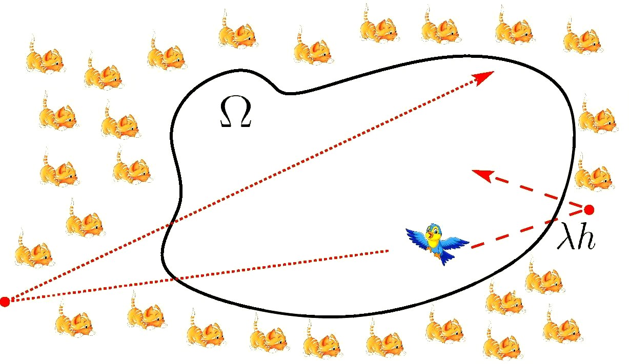
Figure 1.1. Sketch of an ecological niche (the dashed line corresponding to the classical random walk and the dotted line to the jump process).

See Figure 1.1 for a pictorial sketch of the notion of niche that we consider. We observe that the link between reflecting barriers and Neumann conditions is classical in the theory of elliptic partial differential equations (though the topic is often discussed only in dimension $1$, see [MR2399851, page 98]). Reflection of random walks is also classically linked to the so-called Skorokhod problem, see [SKORO1, SKORO2, MR837810]. Also, the relation between jump processes and fractional operators has been widely investigated, see e.g. [MR2512800, MR2584076, MR3967804], and the probabilistic methods often turn out to be extremely profitable in the development of the analytic theory, see e.g. [MR119247, MR1438304, MR2345912]. In our description, for the jump process in $\mathbb{R}^{n}$ we will exploit the description proposed in [MR3469920, Section 2.1], that needs to be combined here with the idea of “immediate return to $\Omega$” that was introduced in [dirova], and whose comprehensive probabilistic setting has been recently provided in [VOND].

Though built on this existing literature, the simple model that we present here comprising both the local and the nonlocal dispersals is new.

As a technical observation, we remark that we are specifically presenting here the case of indistinguishable individuals, each presenting two diffusive patterns with given probabilities: models describing the case of a species with two classes of individuals that present different diffusive patterns (such as the one in [FALCO]) or two species with different diffusive patterns sharing the same ecological niche (as taken into account in [ANT]) are, in a sense, seemingly related to our work, but they are technically quite different.

To appreciate such a difference, one can consider the case in which local searching modes are predominant and consider an evolution in a very large niche starting from a very concentrated initial condition. In this setting, models distinguishing between individuals with short-range and long-range diffusive patterns will find, say, at unit distance from the initial concentration point, after a unit of time, a very small density of short-range travelers (due to the Gaussian decay of the classical heat equation) and a much larger density of long-range travelers (due to the polynomial decay of the nonlocal heat equation) and thus the relative density of short-range travelers in that location will be very small (even if the majority of the population belongs to such a class). Viceversa, in the model that we consider, in the range of parameters in which the local search is predominant, one can expect that short-jumps will happen with high probability among all the individuals who have reached the location.

Interestingly, mixed diffusive patterns can arise from composite stochastic processes, alternating intensive and area-concentrated with extensive and far-reaching search modes, and this diffusive turnover may be induced by environmental features, such as patchy structures, see e.g. [LW]. We also remark that diffusive operators of mixed order naturally arise in probabilistic problems for infinitely divisible distributions via the Lévy-Khintchine formula and find applications in different fields of applied sciences, including phylogeny (see [FILO]) and finance (see [FINA]). We also refer to the monograph [FORA] for a throughout presentation of the theory of random searches for foraging purposes.

Moreover, from the probabilistic perspective, we point out that the distinction between the classical (i.e., Browniann) and the jump (i.e., Lévy) random walks has a natural interpretation in terms of Central Limit Theorems. Namely, the standard random walk meets the Central Limit Theorem in its classical formulation, according to which the sum of a number of independent and identically distributed random variables with finite variances converges to a normal distribution as the number of variables grows. Instead, the jump process meets the “generalized” Central Limit Theorem (see [MR0233400]), according to which the sum of a number of random variables with a power-law tails distributions having infinite variance converges to a stable distribution (and this type of stable distributions present tails that are asymptotically proportional to the ones of a power-law distribution). See e.g. [MR2743162] for further details and a thorough historical review about the Central Limit Theorem, its generalizations and its connections with stable distributions.

We also point out that anomalous diffusion driven by operators of mixed orders (possibly with two fractional terms, as well) has been taken into consideration for the one-dimensional case without boundaries, also in view of the Voigt profile function and of the Mellin-Barnes integrals, and detecting two time-scales of the problem (see equation (3.2) in [MR2459736] or equation (13) in [MR2559350], and [CRME02, CRME08, MR3886705] too). The situation that we take into account here takes somewhat a different point of view, since the boundary and exterior conditions in (1.2) and (1.3) play a decisive role for us in describing the mechanism of egression from, and return to, the given domain.

As a technical remark, we point out that several possible equivalent definitions can be given for the fractional Laplacian introduced in (1.1): for instance, instead of a singular integral operator, one can take into account the generator of a semigroup of operators, or Bochner’s subordination formulas, or Dynkin’s formula, or Riesz potentials, or harmonic extensions, etc. – see e.g. [MR3613319] for a comprehensive treatment of all these possible definitions. Nevertheless, in the scientific literature, other types of fractional versions of the Laplace operators have been taken into account, in terms of censored stochastic processes and spectral analysis. These objects share some traits with the fractional Laplacian in (1.1) here, but they are structurally very different, see in particular [MR3233760, MR3246044] and Sections 2 and 4 in [MR4102340].

Several reasons suggested to us that, among these alternative choices of elliptic fractional operators, the fractional Laplacian in (1.1) was the most convenient one to describe the random egress from a biological niche with immediate return. Indeed, the regional fractional Laplacian (see equation (2.47) in [MR4102340]) acts on functions defined in a given domain, therefore does not seem suitable to take into account the values of the function outside the domain itself (while, for our construction, we need to detect the exterior of the domain, where some egression takes place, though with an instantaneous return to the domain itself). Similarly, the spectral fractional Laplacian (see equation (2.49) in [MR4102340]) acts on functions defined on a given domain, and more specifically on functions in the span of the eigenfunctions of the Laplacian with given boundary conditions: though this setting is adequate for diffusive problems based on the classical heat equation with suitable boundary conditions (see [MR3796372]), not only in this case the function is not naturally defined outside the domain but also the boundary conditions are inherited directly from the local situation and do not take into account the specific features of a long-jump process that we need to take into account in our framework. Conversely, the fractional Laplacian in (1.1) has nice compatibility properties with long-jump processes and produces an exterior condition that can be interpreted naturally as a return to the domain immediately after an egression.

We also point out that, on the one hand, the nonlocal Neumann condition in (1.3) seems to make use of a regional fractional Laplacian with respect to the domain $\Omega$, but, on the other hand, the condition itself takes place in the complement of $\Omega$, hence this prescription does not fall at once into the conventional equations driven by the regional fractional Laplacian (though, as pointed out in [MR4102340, AUD], a regional problem does arise by modifying the kernel with a logarithmic singularity along $\partial\Omega$). The delicate interplay between densities localized in the domain $\Omega$ and quantity globally defined in $\mathbb{R}^{n}$ will play an important role in our construction – for instance, the population density is supposed to be localized in the niche, see (3.1), but a convenient extension of it outside the domain will be taken into account to detect the desired evolution equation, see (3.10), or equivalently one can construct a phantom population outside the domain by a suitable reflection method, see (A.4).

In the forthcoming Section 2, a more precise description of the random process considered will be given. From this, we will formally derive the heat equation (1.1) in Section 3 and the Neumann conditions (1.2)–(1.3) in Section 4. Section 5 summarizes the conclusion of the results presented in this paper.

In the appendix, we will show an alternative approach to the problem, in which the process is defined in the whole of $\mathbb{R}^{n}$.

For the reader’s convenience, before diving into the technical computations of this article, we provide a list of the symbols and conventions adopted in what follows.

Notation table

Notation used	Symbol used	Meaning
Physical space	$\mathbb{R}^{n}$	$\displaystyle{{\mathbb{R}\times\dots\times\mathbb{R}}}$ ($n$ times)
Laplacian	$\Delta$	$\displaystyle\sum_{j=1}^{n}\frac{\partial^{2}}{\partial x_{j}^{2}}$
Fractional power	$s$	a real number between $0$ and $1$
Fractional Laplacian	$-(-\Delta)^{s}u(x)$	$\displaystyle\int_{\mathbb{R}^{n}}\frac{u(y)-u(x)}{|y-x|^{n+2s}}\,dy$
Domain	$\Omega$	a bounded domain in $\mathbb{R}^{n}$ with smooth boundary
External unit normal	$\nu$	unit normal at the boundary of $\Omega$, pointing towards the exterior of $\Omega$
Lebesgue measure	${\mathcal{L}}^{n}$	the standard $n$-dimensional measure
$(n-1)$-dimensional Hausdor measure	${\mathcal{H}}^{n-1}$	the standard surface measure (for hypersurfaces of codimension $1$ in $\mathbb{R}^{n}$)
Unit ball	$B_{1}$	$\{x\in\mathbb{R}^{n}{\mbox{ s.t. }}|x|<1\}$
Unit sphere	$\partial B_{1}$	$\{x\in\mathbb{R}^{n}{\mbox{ s.t. }}|x|=1\}$
Indicator function of a given set $A$	$\chi_{A}$	$\chi_{A}(x):=\begin{cases}1&{\mbox{ if }}x\in A,\cr 0&{\mbox{ otherwise.}}\end{cases}$
Time step	$\tau$	A small real number with the dimensionality of time
Space step	$h$	A small real number with the dimensionality of space
Diffusive parameters	$\alpha$ and $\beta$	Given positive real numbers
Probability of jump process to take place	$p$	Given real number between $0$ and $1$

This notation table lists the symbols mostly used in this paper. Most of this notation is standard, though the literature offers plenty of alternative notation and small variances: for instance, the Laplace operator is sometimes denoted by $\nabla^{2}$ in other papers, the fractional Laplacian by $|\nabla|^{2s}$ and possibly contains normalizing constants, the normal derivative is elsewhere denoted by $n$ (here reserved for the number of dimensions), the infinitesimal volume element of the Lebesgue measure by $dx$, the infinitesimal surface element by $d\sigma$, the fractional parameter $s$ corresponds to $\alpha/2$ in the “$\alpha$-stable” literature in probability and statistics, and the unit sphere is elsewhere often denoted by ${\mathbb{S}}^{n-1}$ especially in differential geometry. We chose the notation stated in the table since we find it more explicit and in order to circumvent unclear statements (especially, we put an effort in distinguishing volume and surface integrals and in avoiding ambiguous notations related to integrals, since the two types of measures play a significantly different role in our framework). Also, as a conceptual simplification, we take our physical space to be $\mathbb{R}^{n}$ rather than restricting to the special cases of $\mathbb{R}$, $\mathbb{R}^{2}$ and $\mathbb{R}^{3}$ (in the case considered here, this higher dimensional generalization does not provide any additional difficulty and does not make the notation heavier).

2. Description of the random process

The probabilistic interpretation of the process leading to equation (1.1) and to the nonlocal Neumann conditions (1.2)–(1.3) goes as follows:

• $u(x,t)$ is the probability distribution of the position of a particle moving randomly in a (say, bounded and smooth) domain $\Omega\subset\mathbb{R}^{n}$;

• The random process followed by the particle is the superposition of a classical random walk and a long-jump random walk. More specifically, we consider a time increment $\tau>0$, a space scale $h>0$, and an additional space parameter $\lambda\in\mathbb{N}$ (in our setting, both $\tau$ and $\lambda h$ will be infinitesimal);

• We assume that the particle has a probability $p$ of following a long-jump process and a probability $1-p$ of following a classical random walk. The probability for the particle of not moving at all is set to be equal to zero. For concreteness, we consider here the case $p\in(0,1)$, but the cases $p=0$ and $p=1$ are comprised in the forthcoming discussion (just focusing on the process allowed by such probability and disregarding the other one);

• When the particle exits $\Omega$, it comes back into $\Omega$ right away. This return to $\Omega$ follows a natural reflection with respect to the random process.

We now discuss the classical random walk and the long jump process more precisely.

2.1. The classical random walk

Concerning the classical random walk, we denote by ${\mathcal{L}}^{n}$ the $n$-dimensional Lebesgue measure, and we describe the probability of walking from $x\in\Omega$ to $y\in\Omega$ as the superposition of these two phenomena:

• the particle can walk “directly” from $x\in\Omega$ to $y\in\Omega$, which occurs with probability density $\frac{\chi_{[0,\lambda h)}(|x-y|)}{{\mathcal{L}}^{n}(B_{\lambda h})}$: that is, each points in the ball $B_{\lambda h}(x)$ are reachable from $x$ with uniform distribution;

• the particle can also walk from $x$ to $y$ “after a reflection” in the complement of $\Omega$: namely, the particle can walk from $x$ to $z\in\mathbb{R}^{n}\setminus\Omega$, which occurs with probability density $\frac{\chi_{[0,\lambda h)}(|x-z|)}{{\mathcal{L}}^{n}(B_{\lambda h})}$, and then walk back instantaneously from $z$ to $y\in\Omega$, and this occurs with probability density $\frac{\chi_{[0,\lambda h)}(|y-z|)}{{\mathcal{L}}^{n}(\Omega\cap B_{\lambda h}(z))}$. That is, the random walk can reach points outside the domain, from which it bounces back to the domain with the same uniform probability law. As a result, the probability density of a reflected walk from $x\in\Omega$ to $y\in\Omega$ is equal to

  $$\int_{\mathbb{R}^{n}\setminus\Omega}\frac{\chi_{[0,\lambda h)}(|x-z|)\;\chi_{[0,\lambda h)}(|y-z|)}{{\mathcal{L}}^{n}(B_{\lambda h})\;{\mathcal{L}}^{n}(\Omega\cap B_{\lambda h}(z))}\,dz.$$

The total probability density of a walk from $x\in\Omega$ to $y\in\Omega$ is therefore the sum of the probabilities of a direct walk and a reflected walk and it is equal to

$$P_{W}(x\to y):=\frac{\chi_{[0,\lambda h)}(|x-y|)}{{\mathcal{L}}^{n}(B_{\lambda h})}+\int_{\mathbb{R}^{n}\setminus\Omega}\frac{\chi_{[0,\lambda h)}(|x-z|)\;\chi_{[0,\lambda h)}(|y-z|)}{{\mathcal{L}}^{n}(B_{\lambda h})\;{\mathcal{L}}^{n}(\Omega\cap B_{\lambda h}(z))}\,dz.$$ (2.1)

We remark that the probability of walking back to the domain after exiting is equal to $1$, since, for every $z\in\mathbb{R}^{n}\setminus\Omega$,

$$\int_{\Omega}\frac{\chi_{[0,\lambda h)}(|y-z|)}{{\mathcal{L}}^{n}(\Omega\cap B_{\lambda h}(z))}\,dy=1.$$

Also, the probability of walking from a given point of $\Omega$ to the domain $\Omega$ itself is equal to $1$, since, for each $x\in\Omega$,

$$\begin{split}&\int_{\Omega}P_{W}(x\to y)\,dy\\ =\,&\int_{\Omega}\frac{\chi_{[0,\lambda h)}(|x-y|)}{{\mathcal{L}}^{n}(B_{\lambda h})}\,dy+\int_{\Omega}\left[\int_{\mathbb{R}^{n}\setminus\Omega}\frac{\chi_{[0,\lambda h)}(|x-z|)\;\chi_{[0,\lambda h)}(|y-z|)}{{\mathcal{L}}^{n}(B_{\lambda h})\;{\mathcal{L}}^{n}(\Omega\cap B_{\lambda h}(z))}\,dz\right]\,dy\\ =\,&\frac{{\mathcal{L}}^{n}(B_{\lambda h}(x)\cap\Omega)}{{\mathcal{L}}^{n}(B_{\lambda h})}+\int_{\mathbb{R}^{n}\setminus\Omega}\left[\int_{\Omega}\frac{\chi_{[0,\lambda h)}(|x-z|)\;\chi_{[0,\lambda h)}(|y-z|)}{{\mathcal{L}}^{n}(B_{\lambda h})\;{\mathcal{L}}^{n}(\Omega\cap B_{\lambda h}(z))}\,dy\right]\,dz\\ =\,&\frac{{\mathcal{L}}^{n}(B_{\lambda h}(x)\cap\Omega)}{{\mathcal{L}}^{n}(B_{\lambda h})}+\int_{\mathbb{R}^{n}\setminus\Omega}\frac{\chi_{[0,\lambda h)}(|x-z|)}{{\mathcal{L}}^{n}(B_{\lambda h})}\,dz\\ =\,&\frac{{\mathcal{L}}^{n}(B_{\lambda h}(x)\cap\Omega)}{{\mathcal{L}}^{n}(B_{\lambda h})}+\frac{{\mathcal{L}}^{n}(B_{\lambda h}(x)\setminus\Omega)}{{\mathcal{L}}^{n}(B_{\lambda h})}\\ =\,&1.\end{split}$$ (2.2)

We also remark that

$$P_{W}(y\to x)=P_{W}(x\to y),$$

thanks to (2.1). This and (2.2) entail that, for every $\eta\in\Omega$,

$$\int_{\Omega}P_{W}(\xi\to\eta)\,d\xi=\int_{\Omega}P_{W}(\eta\to\xi)\,d\xi=1.$$ (2.3)

2.2. The jump process

Concerning the jump process, we denote by ${\mathcal{H}}^{n-1}$ the $(n-1)$-dimensional Hausdorff measure and we let, for all $z\in\mathbb{R}^{n}\setminus\Omega$,

$$\mu_{h}(z):=2s\,h^{2s}\int_{\Omega\setminus B_{h}(z)}\frac{dy}{|y-z|^{n+2s}}.$$ (2.4)

Given $x$, $y\in\Omega$, the probability of jumping from $x$ to $y$ consists in the superposition of two events:

• the particle can jump “directly” from $x$ to $y$: this occurs with probability density

  $$\frac{2s\,h^{2s}\,\chi_{(h,+\infty)}(|x-y|)}{{\mathcal{H}}^{n-1}(\partial B_{1})\;|x-y|^{n+2s}};$$

• the particle can jump from $x$ to $y$ “after a reflection” in the complement of $\Omega$: that is, the particle can jump from $x$ to any point $z\in\mathbb{R}^{n}\setminus\Omega$, which occurs with probability density

  $$\frac{2s\,h^{2s}\,\chi_{(h,+\infty)}(|x-z|)}{{\mathcal{H}}^{n-1}(\partial B_{1})\;|x-z|^{n+2s}},$$

  and then instantaneously back to $\Omega$, that is, from $z$ to $y\in\Omega$, which occurs with probability density

  $$\frac{2s\,h^{2s}\,\chi_{(h,+\infty)}(|y-z|)}{\mu_{h}(z)\;|y-z|^{n+2s}}.$$

  Consequently, the probability density of a reflected jump from $x$ to $y$ passing through $z\in\mathbb{R}^{n}\setminus\Omega$ is obtained by the product rule of independent events, and it is equal to

  $$\int_{\mathbb{R}^{n}\setminus\Omega}\frac{(2s)^{2}\,h^{4s}\,\chi_{(h,+\infty)}(|x-z|)\,\chi_{(h,+\infty)}(|y-z|)}{{\mathcal{H}}^{n-1}(\partial B_{1})\;\mu_{h}(z)\;|x-z|^{n+2s}|y-z|^{n+2s}}\,dz.$$

The probability density of a jump from $x$ to $y$ is therefore the sum of the probability densities of a direct jump and a reflected jump and it is equal to

$$\begin{split}&P_{J}(x\to y):=\frac{2s\,h^{2s}\,\chi_{(h,+\infty)}(|x-y|)}{{\mathcal{H}}^{n-1}(\partial B_{1})\;|x-y|^{n+2s}}+\int_{\mathbb{R}^{n}\setminus\Omega}\frac{(2s)^{2}\,h^{4s}\,\chi_{(h,+\infty)}(|x-z|)\,\chi_{(h,+\infty)}(|y-z|)}{{\mathcal{H}}^{n-1}(\partial B_{1})\;\mu_{h}(z)\;|x-z|^{n+2s}|y-z|^{n+2s}}\,dz.\end{split}$$ (2.5)

We remark that the probability of jumping back to the domain after exiting is equal to $1$, since, for each $z\in\mathbb{R}^{n}\setminus\Omega$,

$$\int_{\Omega}\frac{2s\,h^{2s}\,\chi_{(h,+\infty)}(|y-z|)}{\mu_{h}(z)\;|y-z|^{n+2s}}\,dy=1,$$

thanks to (2.4). In this sense, the return to the domain follows the same jump law of the egress, with the term $\mu_{h}(z)$ acting as a normalization probability factor.

Also, the probability of jumping from a given point of $\Omega$ to the domain $\Omega$ itself is equal to $1$, since, for each $x\in\Omega$,

$$\int_{\Omega}P_{J}(x\to y)\,dy$$

$$= \int_{\Omega}\frac{2s\,h^{2s}\,\chi_{(h,+\infty)}(|x-y|)}{{\mathcal{H}}^{n-1}(\partial B_{1})\;|x-y|^{n+2s}}\,dy+\int_{\Omega}\left[\int_{\mathbb{R}^{n}\setminus\Omega}\frac{(2s)^{2}\,h^{4s}\,\chi_{(h,+\infty)}(|x-z|)\,\chi_{(h,+\infty)}(|y-z|)}{{\mathcal{H}}^{n-1}(\partial B_{1})\;\mu_{h}(z)\;|x-z|^{n+2s}|y-z|^{n+2s}}\,dz\right]\,dy$$

$$= \frac{2s\,h^{2s}}{{\mathcal{H}}^{n-1}(\partial B_{1})}\int_{\Omega\setminus B_{h}(x)}\frac{dy}{|x-y|^{n+2s}}+\int_{\mathbb{R}^{n}\setminus\Omega}\left[\int_{\Omega}\frac{(2s)^{2}\,h^{4s}\,\chi_{(h,+\infty)}(|x-z|)\,\chi_{(h,+\infty)}(|y-z|)}{{\mathcal{H}}^{n-1}(\partial B_{1})\;\mu_{h}(z)\;|x-z|^{n+2s}|y-z|^{n+2s}}\,dy\right]\,dz$$

$$= \frac{2s\,h^{2s}}{{\mathcal{H}}^{n-1}(\partial B_{1})}\int_{\Omega\setminus B_{h}(x)}\frac{dy}{|x-y|^{n+2s}}+\int_{\mathbb{R}^{n}\setminus\Omega}\frac{2s\,h^{2s}\,\chi_{(h,+\infty)}(|x-z|)}{{\mathcal{H}}^{n-1}(\partial B_{1})\;|x-z|^{n+2s}}\,dz$$

$$= \frac{2s\,h^{2s}}{{\mathcal{H}}^{n-1}(\partial B_{1})}\left[\int_{\Omega\setminus B_{h}(x)}\frac{dy}{|x-y|^{n+2s}}+\int_{(\mathbb{R}^{n}\setminus\Omega)\setminus B_{h}(x)}\frac{dz}{|x-z|^{n+2s}}\right]$$

$$= \frac{2s\,h^{2s}}{{\mathcal{H}}^{n-1}(\partial B_{1})}\int_{\mathbb{R}^{n}\setminus B_{h}(x)}\frac{d\xi}{|x-\xi|^{n+2s}}$$

$$= 2s\,h^{2s}\int_{h}^{+\infty}\frac{d\rho}{\rho^{1+2s}}$$

$$= 1.$$

Since $P_{J}(y\to x)=P_{J}(x\to y)$, due to (2.5), we also have that, for all $x\in\Omega$,

$$\int_{\zeta\in\Omega}P_{J}(\zeta\to x)\,d{\mathcal{H}}^{n-1}_{\zeta}=1.$$ (2.6)

Following [VERO], we consider here the special sets of parameters

$$\tau:=h^{2s},\qquad\lambda:=h^{s-1}\in\mathbb{N},\qquad{\mbox{ and~{}$p$ is independent of $h$}}$$ (2.7)

and we describe in detail how these prescriptions lead to a heat equation of mixed local and nonlocal type as in (1.1), with nonlocal Neumann conditions as in (1.2)–(1.3). These aspects will be discussed in the forthcoming sections.

3. The heat equation

We denote by $u(x,t)$ the total probability density for the particle to be at the point $x$ at time $t$, and we set

$$u_{J}(x,t):=p\,u(x,t)\qquad{\mbox{ and }}\qquad u_{W}(x,t):=(1-p)\,u(x,t).$$

Roughly speaking, one can consider $u_{W}$ (respectively, $u_{J}$) to be the contribution of probability density for the particle to be at the point $x\in\Omega$ at time $t\in\tau\mathbb{N}$ coming from the classical random walk (respectively, the jump process). By construction, both the classical random walk and the jump process do not leave the domain $\Omega$, hence we can write that

$$u(x,t)=u_{W}(x,t)=u_{J}(x,t)=0\qquad{\mbox{ whenever }}\,x\not\in\Omega.$$ (3.1)

Moreover,

$$u(x,t)=u_{J}(x,t)+u_{W}(x,t).$$ (3.2)

Given $x\in\Omega$, the probability of being at $x$ at time $t+\tau$ is the superposition of the probability of being at any other point $y\in\Omega$ at time $t$, times the probability $P(y\mapsto x)$ of jumping from $y$ to $x$. For this reason, we write

$$u(x,t+\tau)=\int_{\Omega}u(y,t)\,P(y\mapsto x)\,dy.$$ (3.3)

By the random processes described in Sections 2.1 and 2.2, we have that

$$P(y\mapsto x)=p\,P_{J}(y\mapsto x)+(1-p)\,P_{W}(y\mapsto x),$$ (3.4)

and consequently, by (2.3) and (2.6),

$$\int_{\Omega}P(y\mapsto x)\,dy=1.$$

This and (3.3) lead to

$$\frac{u(x,t+\tau)-u(x,t)}{\tau}=\int_{\Omega}\frac{u(y,t)-u(x,t)}{\tau}\,P(y\mapsto x)\,dy.$$

As a result, by (3.2) and (3.4),

$$\begin{split}&\left[\frac{u_{W}(x,t+\tau)-u_{W}(x,t)}{\tau}-(1-p)\int_{\Omega}\frac{u(y,t)-u(x,t)}{\tau}\,P_{W}(y\mapsto x)\,dy\right]\\ &\qquad+\left[\frac{u_{J}(x,t+\tau)-u_{J}(x,t)}{\tau}-p\int_{\Omega}\frac{u(y,t)-u(x,t)}{\tau}\,P_{J}(y\mapsto x)\,dy\right]\\ =\,&\frac{u(x,t+\tau)-u(x,t)}{\tau}-\int_{\Omega}\frac{u(y,t)-u(x,t)}{\tau}\,P(y\mapsto x)\,dy=0.\end{split}$$ (3.5)

We denote by ${\mathcal{T}}_{W}(x,t)$ (respectively, ${\mathcal{T}}_{J}(x,t)$) the item in the first (respectively, the second) square brackets in (3.5).

Recalling (2.1), we know that, for every $x\in\Omega$ with $B_{\lambda h}(x)\Subset\Omega$,

$$P_{W}(x\to y) = \frac{\chi_{[0,\lambda h)}(|x-y|)}{{\mathcal{L}}^{n}(B_{\lambda h})}+\int_{\mathbb{R}^{n}\setminus\Omega}\frac{\chi_{[0,\lambda h)}(|x-z|)\;\chi_{[0,\lambda h)}(|y-z|)}{{\mathcal{L}}^{n}(B_{\lambda h})\;{\mathcal{L}}^{n}(\Omega\cap B_{\lambda h}(z))}\,dz$$

$$= \frac{\chi_{[0,\lambda h)}(|x-y|)}{{\mathcal{L}}^{n}(B_{\lambda h})},$$

since the integration set over $z$ is empty.

Thus, for every $x\in\Omega$ with $B_{\lambda h}(x)\Subset\Omega$,

$${\mathcal{T}}_{W}(x,t)=\frac{u_{W}(x,t+\tau)-u_{W}(x,t)}{\tau}-\frac{1-p}{{\mathcal{L}}^{n}(B_{\lambda h})}\int_{B_{\lambda h}(x)}\frac{u(y,t)-u(x,t)}{\tau}\,dy.$$ (3.6)

Furthermore, using that $\lambda h=\sqrt{\tau}$, due to (2.7), if $y\in B_{\lambda h}(x)$, a formal Taylor expansion leads to

$$u(y,t) = u(x,t)+\nabla u(x,t)\cdot(y-x)+\frac{1}{2}\,D^{2}u(x,t)(x-y)\cdot(x-y)+O(|x-y|^{3})$$

$$= u(x,t)+\nabla u(x,t)\cdot(y-x)+\frac{1}{2}\,\sum_{i,j=1}^{n}\partial^{2}_{ij}u(x,t)(x_{i}-y_{i})(x_{j}-y_{j})+O(\tau^{3/2}).$$

This, together with two odd symmetry cancellations, gives that

$$\int_{B_{\lambda h}(x)}\frac{u(y,t)-u(x,t)}{\tau}\,dy$$

$$= \frac{1}{\tau}\int_{B_{\sqrt{\tau}}(x)}\left[\nabla u(x,t)\cdot(y-x)+\frac{1}{2}\,\sum_{i,j=1}^{n}\partial^{2}_{ij}u(x,t)(x-y)\cdot(x-y)\right]\,dy+O\left(\tau^{\frac{n+1}{2}}\right)$$

$$= \sum_{i,j=1}^{n}\frac{\partial^{2}_{ij}u(x,t)}{2\tau}\int_{B_{\sqrt{\tau}}(x)}(x_{i}-y_{i})(x_{j}-y_{j})\,dy+O\left(\tau^{\frac{n+1}{2}}\right)$$

$$= \sum_{i,j=1}^{n}\frac{\tau^{\frac{n}{2}}\partial^{2}_{ij}u(x,t)}{2}\int_{B_{1}}\omega_{i}\omega_{j}\,d\omega+O\left(\tau^{\frac{n+1}{2}}\right)$$

$$= \sum_{i=1}^{n}\frac{\tau^{\frac{n}{2}}\partial^{2}_{i}u(x,t)}{2}\int_{B_{1}}\omega_{i}^{2}\,d\omega+O\left(\tau^{\frac{n+1}{2}}\right).$$

Consequently, since, for each $i\in\{1,\dots,n\}$,

$$c_{o}:=\int_{B_{1}}|\omega|^{2}\,d\omega=\sum_{j=1}^{n}\int_{B_{1}}\omega_{j}^{2}\,d\omega=n\int_{B_{1}}\omega_{i}^{2}\,d\omega,$$

we find that

$$\int_{B_{\lambda h}(x)}\frac{u(y,t)-u(x,t)}{\tau}\,dy=\sum_{i=1}^{n}\frac{c_{o}\;\tau^{\frac{n}{2}}\partial^{2}_{i}u(x,t)}{2n}+O\left(\tau^{\frac{n+1}{2}}\right)=\frac{c_{o}\;\tau^{\frac{n}{2}}\Delta u(x,t)}{2n}+O\left(\tau^{\frac{n+1}{2}}\right).$$

Thus, plugging this information into (3.6), we obtain

$${\mathcal{T}}_{W}(x,t) = \frac{u_{W}(x,t+\tau)-u_{W}(x,t)}{\tau}-\frac{1-p}{{\mathcal{L}}^{n}(B_{\sqrt{\tau}})}\left[\frac{c_{o}\;\tau^{\frac{n}{2}}\Delta u(x,t)}{2n}+O\left(\tau^{\frac{n+1}{2}}\right)\right]$$

$$= \frac{u_{W}(x,t+\tau)-u_{W}(x,t)}{\tau}-\frac{1-p}{{\mathcal{L}}^{n}(B_{1})}\left[\frac{c_{o}\;\Delta u(x,t)}{2n}+O(\sqrt{\tau})\right].$$

Passing to the limit the previous identity, we thereby formally conclude that, for all $x\in\Omega$,

$$\lim_{h\to 0}{\mathcal{T}}_{W}(x,t)=\partial_{t}u_{W}(x,t)-(1-p)\,\Delta u(x,t),$$ (3.7)

up to neglecting normalization constants.

As for the contributions coming from the jump process, recalling (2.7), we see that

$${\mathcal{T}}_{J}(x,t)=\frac{u_{J}(x,t+\tau)-u_{J}(x,t)}{\tau}-p\int_{\Omega}\frac{u(y,t)-u(x,t)}{h^{2s}}\,P_{J}(y\mapsto x)\,dy.$$ (3.8)

Moreover, in light of (2.5),

$$\begin{split}&\int_{\Omega}\frac{u(y,t)-u(x,t)}{h^{2s}}\,P_{J}(y\mapsto x)\,dy\\ =\;&\int_{\Omega}\frac{u(y,t)-u(x,t)}{h^{2s}}\,\Bigg{\{}\frac{2s\,h^{2s}\,\chi_{(h,+\infty)}(|x-y|)}{{\mathcal{H}}^{n-1}(\partial B_{1})\;|x-y|^{n+2s}}\\ &\qquad+\int_{\mathbb{R}^{n}\setminus\Omega}\frac{(2s)^{2}\,h^{4s}\,\chi_{(h,+\infty)}(|x-z|)\,\chi_{(h,+\infty)}(|y-z|)}{{\mathcal{H}}^{n-1}(\partial B_{1})\;\mu_{h}(z)\;|x-z|^{n+2s}|y-z|^{n+2s}}\,dz\Bigg{\}}\,dy\\ =\;&\frac{2s}{{\mathcal{H}}^{n-1}(\partial B_{1})}\,\big{(}I_{h}+J_{h}\big{)},\end{split}$$ (3.9)

where

$$I_{h} := \int_{\Omega\setminus B_{h}(x)}\frac{u(y,t)-u(x,t)}{|x-y|^{n+2s}}\,dy$$

$${\mbox{and }}\quad J_{h} := 2s\,h^{2s}\int_{\Omega}\left[\int_{\mathbb{R}^{n}\setminus\Omega}\frac{\big{(}u(y,t)-u(x,t)\big{)}\;\chi_{(h,+\infty)}(|x-z|)\,\chi_{(h,+\infty)}(|y-z|)}{\mu_{h}(z)\;|x-z|^{n+2s}|y-z|^{n+2s}}\,dz\right]\,dy.$$

It is now convenient to set

$$\begin{split}&U(x,t):=\begin{dcases}u(x,t)&{\mbox{ if }}x\in\overline{\Omega},\\ \\ \frac{\displaystyle\int_{\Omega}\frac{u(y,t)}{|x-y|^{n+2s}}\,dy}{\displaystyle\int_{\Omega}\frac{dy}{|x-y|^{n+2s}}}&{\mbox{ if }}x\in\mathbb{R}^{n}\setminus\overline{\Omega}\end{dcases}\end{split}$$ (3.10)

and

$$\begin{split}&U_{h}(x,t):=\begin{dcases}u(x,t)&{\mbox{ if }}x\in\overline{\Omega},\\ \\ \frac{\displaystyle\int_{\Omega\setminus B_{h}(x)}\frac{u(y,t)}{|x-y|^{n+2s}}\,dy}{\displaystyle\int_{\Omega\setminus B_{h}(x)}\frac{dy}{|x-y|^{n+2s}}}&{\mbox{ if }}x\in\mathbb{R}^{n}\setminus\overline{\Omega}.\end{dcases}\end{split}$$ (3.11)

In some sense, the setting in (3.10) can be seen as a “nonlocal variant” of the classical “method of images” (see e.g. page 28 in [MR3380662] or Chapter 2 in [ELEME]), in which one defines a “phantom” population outside the niche, to keep the population balance constant in the niche.

With this notation, and recalling the definition of $\mu_{h}$ in (2.4), we observe that, for all $x\in\Omega$,

$$J_{h} := \int_{(\mathbb{R}^{n}\setminus\Omega)\setminus B_{h}(x)}\left[\int_{\Omega\setminus B_{h}(z)}\frac{u(y,t)-u(x,t)}{\displaystyle\int_{\Omega\setminus B_{h}(z)}\frac{dw}{|w-z|^{n+2s}}\;|y-z|^{n+2s}}\,dy\right]\,\frac{dz}{|x-z|^{n+2s}}$$

$$= \int_{(\mathbb{R}^{n}\setminus\Omega)\setminus B_{h}(x)}\big{(}U_{h}(z,t)-U_{h}(x,t)\big{)}\,\frac{dz}{|x-z|^{n+2s}}.$$

Hence, since

$$U_{h}(x,t)\longrightarrow U(x,t)\qquad\qquad{\mbox{as }}\,h\to 0,$$ (3.12)

we formally obtain that

$$\lim_{h\to 0}(I_{h}+J_{h})=\int_{\mathbb{R}^{n}}\big{(}U(z,t)-U(x,t)\big{)}\,\frac{dz}{|x-z|^{n+2s}}=-(-\Delta)^{s}U(x,t),$$

up to neglecting normalization constants.

From this and (3.9), we deduce that

$$\lim_{h\to 0}\int_{\Omega}\frac{u(y,t)-u(x,t)}{h^{2s}}\,P_{J}(y\mapsto x)\,dy=-(-\Delta)^{s}U(x,t),$$

up to neglecting normalization constants once again.

This and (3.8) lead to

$$\lim_{h\to 0}{\mathcal{T}}_{J}(x,t)=\partial_{t}u_{J}(x,t)+p(-\Delta)^{s}U(x,t).$$

From this, (3.5) and (3.7), and omitting constants again, we find, when $x\in\Omega$,

$$0 = \lim_{h\to 0}{\mathcal{T}}_{W}(x,t)+{\mathcal{T}}_{J}(x,t)$$

$$= \partial_{t}u_{W}(x,t)-(1-p)\Delta u(x,t)+\partial_{t}u_{J}(x,t)+p(-\Delta)^{s}U(x,t)$$

$$= \partial_{t}u(x,t)-(1-p)\Delta u(x,t)+p(-\Delta)^{s}U(x,t)$$

$$= \partial_{t}U(x,t)-(1-p)\Delta U(x,t)+p(-\Delta)^{s}U(x,t),$$

which is the desired heat equation in (1.1).

4. The Neumann condition

We suppose, up to a translation, that the origin lies in an $h$-neighborhood of the boundary of $\Omega$ – in fact, for simplicity, let us just suppose that $0\in\partial\Omega$ and let $\nu$ be the external unit normal of $\Omega$.

The probability density of finding the particle at $x\in\Omega$ at time $t+\tau$ can be written as in (3.3), thus leading to (3.5). We will therefore exploit (3.5) in this setting, that we write in the form

$$\begin{split}&\left[\frac{u_{W}(x,t+\tau)-u_{W}(x,t)}{\lambda h}-(1-p)\int_{\Omega}\frac{u(y,t)-u(x,t)}{\lambda h}\,P_{W}(y\mapsto x)\,dy\right]\\ &\qquad+\left[\frac{u_{J}(x,t+\tau)-u_{J}(x,t)}{\lambda h}-p\int_{\Omega}\frac{u(y,t)-u(x,t)}{\lambda h}\,P_{J}(y\mapsto x)\,dy\right]=0.\end{split}$$ (4.1)

We denote by ${\mathcal{S}}_{W}(x,t)$ (respectively, ${\mathcal{S}}_{J}(x,t)$) the item in the first (respectively, the second) square brackets in (4.1).

Our goal is now to exploit suitable expansions of the function $u(x,t)$ to relate it to the mixed fractional equation (1.1). For this, we will relate this function to stable densities, and specifically the term ${\mathcal{S}}_{W}$ will correspond to a local diffusive operator while the term ${\mathcal{S}}_{J}$ to a fractional one. Indeed, the Brownian probability term $P_{W}$, acting on a short range and being invariant under rotations and translations, will produce in the limit the Laplace operator, which constitutes the Gaussian contribution of the evolution equation in (1.1). Instead, the power-law probability term $P_{J}$ will maintain its long tail in the limit and produce the fractional Laplace operator, which constitutes the Lévy contribution of (1.1).

More precisely, we notice that, if $y\in\overline{B_{2\lambda h}(x)}$, with a formal Taylor expansion we can write that

$$u(y,t)-u(x,t)=\nabla u(x,t)\cdot(y-x)+O(|x-y|^{2})=\nabla u(x,t)\cdot(y-x)+O(\lambda^{2}h^{2}).$$

We also remark that, due to the construction of the random walk in Section 2.1, the function $y\mapsto P_{W}(y\mapsto x)$ is supported in $y\in\overline{B_{2\lambda h}(x)}$, and, as a result, for all $y\in\mathbb{R}^{n}$ we have that

$$\big{(}u(y,t)-u(x,t)\big{)}\,P_{W}(y\mapsto x)=\Big{(}\nabla u(x,t)\cdot(y-x)+O(\lambda^{2}h^{2})\Big{)}P_{W}(y\mapsto x).$$

This gives that

$${\mathcal{S}}_{W}(x,t)=\frac{u_{W}(x,t+\tau)-u_{W}(x,t)}{\lambda h}-(1-p)\int_{\Omega}\left(\frac{\nabla u(x,t)\cdot(y-x)}{\lambda h}+O(\lambda h)\right)\,P_{W}(y\mapsto x)\,dy.$$

Also, in light of (2.7), another formal Taylor expansion gives that

$$\frac{u_{W}(x,t+\tau)-u_{W}(x,t)}{\lambda h}=\frac{O(\tau)}{\lambda h}=O(h^{s}),$$ (4.2)

and therefore

$${\mathcal{S}}_{W}(x,t)=-(1-p)\int_{\Omega}\frac{\nabla u(x,t)\cdot(y-x)}{\lambda h}\,P_{W}(y\mapsto x)\,dy+O(h^{s}).$$ (4.3)

As a consequence, recalling (2.1),

$$\begin{split}{\mathcal{S}}_{W}(x,t)=\,&-\frac{1-p}{{\mathcal{L}}^{n}(B_{1})}\int_{\Omega}\frac{\nabla u(x,t)\cdot(y-x)}{(\lambda h)^{n+1}}\,\Bigg{[}\chi_{[0,\lambda h)}(|x-y|)\\ &\qquad\qquad+\int_{\mathbb{R}^{n}\setminus\Omega}\frac{\chi_{[0,\lambda h)}(|x-z|)\;\chi_{[0,\lambda h)}(|y-z|)}{{\mathcal{L}}^{n}(\Omega\cap B_{\lambda h}(z))}\,dz\Bigg{]}\,dy+O(h^{s})\\ =\,&-\frac{1-p}{{\mathcal{L}}^{n}(B_{1})}\Bigg{[}\int_{\Omega\cap B_{\lambda h}(x)}\frac{\nabla u(x,t)\cdot(y-x)}{(\lambda h)^{n+1}}\,dy\\ &\qquad+\int_{(\mathbb{R}^{n}\setminus\Omega)\cap B_{\lambda h}(x)}\left(\int_{\Omega\cap B_{\lambda h}(z)}\frac{\nabla u(x,t)\cdot(y-x)}{(\lambda h)^{n+1}\,{\mathcal{L}}^{n}(\Omega\cap B_{\lambda h}(z))}\,dy\right)\,dz\Bigg{]}+O(h^{s})\\ =\,&-\frac{1-p}{{\mathcal{L}}^{n}(B_{1})}\Bigg{[}\int_{\frac{\Omega-x}{\lambda h}\cap B_{1}}\nabla u(x,t)\cdot Y\,dY\\ &\qquad+\int_{\frac{(\mathbb{R}^{n}\setminus\Omega)-x}{\lambda h}\cap B_{1}}\left(\int_{\Big{(}\frac{\Omega-x}{\lambda h}-Z\Big{)}\cap B_{1}}\frac{\nabla u(x,t)\cdot(Y+Z)}{{\mathcal{L}}^{n}\left(\Big{(}{\frac{\Omega-x}{\lambda h}-Z\Big{)}\cap B_{1}}\right)}\,dY\right)\,dZ\Bigg{]}+O(h^{s}).\end{split}$$ (4.4)

Now we consider the jump process and we exploit (4.2) (with $u_{J}$ in place of $u_{W}$), thus obtaining that

$${\mathcal{S}}_{J}(x,t)=-p\int_{\Omega}\frac{u(y,t)-u(x,t)}{\lambda h}\,P_{J}(y\mapsto x)\,dy+O(h^{s}).$$ (4.5)

Recalling the definition of $\mu_{h}$ in (2.4) and that of $U_{h}$ in (3.11), we also observe that

$$E_{h} := \int_{\Omega}\left[\int_{\mathbb{R}^{n}\setminus\Omega}\frac{2s\,h^{4s}\,\chi_{(h,+\infty)}(|x-z|)\,\chi_{(h,+\infty)}(|y-z|)\;\big{(}u(y,t)-u(x,t)\big{)}}{\lambda h\;\mu_{h}(z)\;|x-z|^{n+2s}|y-z|^{n+2s}}\,dz\right]\,dy$$

$$= \int_{(\mathbb{R}^{n}\setminus\Omega)\setminus B_{h}(x)}\left[\int_{\Omega\setminus B_{h}(z)}\frac{h^{2s}\,\big{(}u(y,t)-u(x,t)\big{)}}{\lambda h\;\displaystyle\int_{\Omega\setminus B_{h}(z)}\frac{dw}{|w-z|^{n+2s}}\;|x-z|^{n+2s}|y-z|^{n+2s}}\,dy\right]\,dz$$

$$= \int_{(\mathbb{R}^{n}\setminus\Omega)\setminus B_{h}(x)}\frac{h^{2s}\,\big{(}U_{h}(z,t)-U_{h}(x,t)\big{)}}{\lambda h\;|x-z|^{n+2s}}\,dz.$$

Formally assuming sufficient regularity for $U_{h}$, we write that

$$\big{|}U_{h}(z,t)-U_{h}(x,t)\big{|}\leqslant C\,\min\{1,|x-z|\}$$

for some $C>0$, whence, by the parameters’ choice in (2.7),

$$|E_{h}| \leqslant C\,h^{s}\int_{\mathbb{R}^{n}\setminus B_{h}(x)}\frac{\min\{1,|x-z|\}}{|x-z|^{n+2s}}\,dz$$

$$= C\,h^{s}\int_{B_{1}(x)\setminus B_{h}(x)}\frac{dz}{|x-z|^{n+2s-1}}+O(h^{s})$$

$$= O(h^{1-s})+O(h^{s})+O(h^{1/2}|\ln h|).$$

From this and (2.5), and possibly renaming $C>0$, we deduce that

$$\left|\int_{\Omega}\frac{u(y,t)-u(x,t)}{\lambda h}\,P_{J}(y\mapsto x)\,dy\right|\leqslant\int_{\Omega\setminus B_{h}(x)}\frac{2s\,h^{2s}\,\big{|}u(y,t)-u(x,t)\big{|}}{\lambda h\;{\mathcal{H}}^{n-1}(\partial B_{1})\;|x-y|^{n+2s}}\,dy+\frac{2s\;|E_{h}|}{{\mathcal{H}}^{n-1}(\partial B_{1})}$$

$$\qquad\leqslant Ch^{s}\int_{\Omega\setminus B_{h}(x)}\frac{dy}{|x-y|^{n+2s-1}}+O(h^{1-s})+O(h^{s})+O(h^{1/2}|\ln h|)$$

$$\qquad=O(h^{1-s})+O(h^{s})+O(h^{1/2}|\ln h|).$$

As a consequence, we infer from (4.5) that

$${\mathcal{S}}_{J}(x,t)=O(h^{1-s})+O(h^{s})+O(h^{1/2}|\ln h|).$$

From this, (4.1) and (4.4) we get that

$$\begin{split}&\int_{\frac{\Omega-x}{\lambda h}\cap B_{1}}\nabla U(x,t)\cdot Y\,dY+\int_{\frac{(\mathbb{R}^{n}\setminus\Omega)-x}{\lambda h}\cap B_{1}}\left(\int_{\Big{(}\frac{\Omega-x}{\lambda h}-Z\Big{)}\cap B_{1}}\frac{\nabla U(x,t)\cdot(Y+Z)}{{\mathcal{L}}^{n}\left(\Big{(}{\frac{\Omega-x}{\lambda h}-Z\Big{)}\cap B_{1}}\right)}\,dY\right)\,dZ\\ &\qquad\qquad\qquad=O(h^{1-s})+O(h^{s})+O(h^{1/2}|\ln h|).\end{split}$$

In particular, taking the formal limit as $x\to 0$,

$$\begin{split}&\int_{\frac{\Omega}{\lambda h}\cap B_{1}}\nabla U(0,t)\cdot Y\,dY+\int_{\frac{\mathbb{R}^{n}\setminus\Omega}{\lambda h}\cap B_{1}}\left(\int_{\Big{(}\frac{\Omega}{\lambda h}-Z\Big{)}\cap B_{1}}\frac{\nabla U(0,t)\cdot(Y+Z)}{{\mathcal{L}}^{n}\left(\Big{(}{\frac{\Omega}{\lambda h}-Z\Big{)}\cap B_{1}}\right)}\,dY\right)\,dZ\\ &\qquad\qquad\qquad=O(h^{1-s})+O(h^{s})+O(h^{1/2}|\ln h|).\end{split}$$ (4.6)

Now we observe that, as $h\to 0$, the rescaled domain $\frac{\Omega}{\lambda h}$ approaches the halfspace $\Pi$ through the origin with external normal $\nu(0)$.

As a result, we take the formal limit as $h\to 0$ of the identity in (4.6), gathering that

$$\int_{\Pi\cap B_{1}}\nabla U(0,t)\cdot Y\,dY+\int_{(\mathbb{R}^{n}\setminus\Pi)\cap B_{1}}\left(\int_{\Big{(}\Pi-Z\Big{)}\cap B_{1}}\frac{\nabla U(0,t)\cdot(Y+Z)}{{\mathcal{L}}^{n}\left(\Big{(}{\Pi-Z\Big{)}\cap B_{1}}\right)}\,dY\right)\,dZ=0.$$ (4.7)

Now we claim that

$$\int_{\Pi\cap B_{1}}Y\,dY+\int_{(\mathbb{R}^{n}\setminus\Pi)\cap B_{1}}\left(\int_{\Big{(}\Pi-Z\Big{)}\cap B_{1}}\frac{Y+Z}{{\mathcal{L}}^{n}\left(\Big{(}{\Pi-Z\Big{)}\cap B_{1}}\right)}\,dY\right)\,dZ=-c_{\star}\,\nu(0),$$ (4.8)

for some $c_{\star}>0$. To prove this, up to a rotation, we suppose that $\nu(0)=(0,\dots,0,1)$, whence $\Pi=\{\zeta=(\zeta_{1},\dots,\zeta_{n})\in\mathbb{R}^{n}{\mbox{ s.t. }}\zeta_{n}<0\}$. Therefore, the $n$th component of the left hand side of (4.8) is

$$\int_{\{Y_{n}<0\}\cap B_{1}}Y_{n}\,dY+\int_{\{Z_{n}>0\}\cap B_{1}}\left(\int_{\Big{(}\{Y_{n}<0\}-Z\Big{)}\cap B_{1}}\frac{Y_{n}+Z_{n}}{{\mathcal{L}}^{n}\left(\Big{(}{\{Y_{n}<0\}-Z\Big{)}\cap B_{1}}\right)}\,dY\right)\,dZ,$$

which is strictly negative, say equal to $-c_{\star}$ for some $c_{\star}>0$, since both the numerators in the above integrals are negative.

Also, for each $i\in\{1,\dots,n-1\}$, the $i$th component of the left hand side of (4.8) is

$$\int_{\{Y_{n}<0\}\cap B_{1}}Y_{i}\,dY+\int_{\{Z_{n}>0\}\cap B_{1}}\left(\int_{\Big{(}\{Y_{n}<0\}-Z\Big{)}\cap B_{1}}\frac{Y_{i}+Z_{i}}{{\mathcal{L}}^{n}\left(\Big{(}{\{Y_{n}<0\}-Z\Big{)}\cap B_{1}}\right)}\,dY\right)\,dZ,$$

which is equal to zero, since the integrands are odd with respect to the $i$th variable, while the domains remain the same after switching $Y_{i}$ to $-Y_{i}$ and $Z_{i}$ to $-Z_{i}$.

These considerations lead to

$$\int_{\Pi\cap B_{1}}Y\,dY+\int_{(\mathbb{R}^{n}\setminus\Pi)\cap B_{1}}\left(\int_{\Big{(}\Pi-Z\Big{)}\cap B_{1}}\frac{Y+Z}{{\mathcal{L}}^{n}\left(\Big{(}{\Pi-Z\Big{)}\cap B_{1}}\right)}\,dY\right)\,dZ$$

$$\qquad=(0,\dots,0,-c_{\star})=-c_{\star}\,\nu(0),$$

and this proves (4.8), as desired.

By (4.7) and (4.8) we deduce that

$$-c_{\star}\,\nabla U(0,t)\cdot\nu(0)=0,$$

that is $\partial_{\nu}U(0,t)=0$. Since the origin was an arbitrary point of $\partial\Omega$, we have thus obtained the local Neumann prescription in (1.2).

Furthermore, using (3.10), we see that the nonlocal Neumann prescription in (1.3) is fulfilled in $\mathbb{R}^{n}\setminus\overline{\Omega}$, as desired.

5. Conclusions

We have proposed a mathematical description of an ecological model, by also providing concrete motivations. The model has been described precisely at an intuitive level, with explicit calculations that can be followed without many prerequisites.

The model describes a biological population which can pursue both a classical (i.e. Brownian) and a long-range (i.e. Lévy) dispersal strategies and lives in an ecological niche. In this situation, the combination of Brownian and Lévy processes produces an evolution equation similar to the heat flow but with the Laplace operator replaced by the superposition of a Laplacian and a fractional Laplacian.

The equation is set in a domain (which corresponds to the biological niche). Additionally, in view of this combination of different types of diffusion, a new type of Neumann condition is needed to impose a zero-flux prescription of the niche and model the return to the niche after a possible egress due to a stochastic process. This new type of Neumann condition is also a superposition of the classical Neumann condition (prescribing the normal derivative at the boundary of the domain) and of a fractional Neumann condition (corresponding to an integral relation in the complement of the domain).

The analytic approach to this model can provide inspiration for further understanding of biological situations of interest.

Appendix A The “point of view of the niche”

It is interesting to point out that the function $U$ introduced in (3.10) gives a possible different interpretation of the stochastic process, providing an equivalent setting defined in the whole of $\mathbb{R}^{n}$ and not only in $\Omega$ (remarkably, also in [VOND] a rigorous approach is provided to define a random process in $\mathbb{R}^{n}$ equivalent to the one producing the Neumann condition of [dirova]).

That is, one could define

$$d\pi_{W}(y;x):=\frac{\chi_{[0,\lambda h)}(|x-y|)}{{\mathcal{L}}^{n}(B_{\lambda h})}\,dy$$ (A.1)

and

$$d\pi_{J}(y;x):=\frac{2s\,h^{2s}\,\chi_{(h,+\infty)}(|x-y|)}{{\mathcal{H}}^{n-1}(\partial B_{1})\;|x-y|^{n+2s}}\,dy.$$ (A.2)

In a sense, the quantity in (A.1) is induced by the random walk probability density described in Section 2.1, and the quantity in (A.2) is coming from the jump process probability density described in Section 2.2. It is also worth pointing out that the processes in (A.1) and (A.2) somewhat “complement” each other, since the first takes care of short-range movements at distance less than $\lambda h$ and the latter produces trajectories that are always longer than $h$.

We will now complement these objects by a suitable “method of images”. Namely, we set

$$d\pi(y;x):=p\,d\pi_{J}(y;x)+(1-p)\,d\pi_{W}(y;x)$$ (A.3)

and

$$\Omega^{(\lambda h)}:=\{x\in\Omega{\mbox{ s.t. }}B_{\lambda h}(x)\Subset\Omega\},$$

and we could consider $V$ as the density of a biological population in $\Omega$ and that of a “phantom” population $V_{h}$ outside $\Omega^{(\lambda h)}$, assuming that such a population is subject to a random process, with probability density of jump from $y\in\mathbb{R}^{n}$ to $x\in\Omega^{(\lambda h)}$ given by (A.3); the phantom population is then reset to the appropriate value in (3.10) outside $\Omega^{(\lambda h)}$ at each time step of the process. Namely, while the process occurs in $\Omega^{(\lambda h)}$, the diffusing density is defined outside $\Omega^{(\lambda h)}$ by

$$V_{h}(x,t):=\begin{dcases}V(x,t)&{\mbox{ if }}x\in\Omega^{(\lambda h)},\\ \\ \displaystyle\frac{\displaystyle\int_{\Omega\cap B_{\lambda h}(x)}V(y,t)\,dy}{\displaystyle{\mathcal{L}}^{n}(\Omega\cap B_{\lambda h}(x))}&{\mbox{ if }}x\in\overline{\Omega}\setminus\Omega^{(\lambda h)},\\ \\ \frac{\displaystyle\int_{\Omega}\frac{V(y,t)}{|x-y|^{n+2s}}\,dy}{\displaystyle\int_{\Omega}\frac{dy}{|x-y|^{n+2s}}}&{\mbox{ if }}x\in\mathbb{R}^{n}\setminus\overline{\Omega}.\end{dcases}$$ (A.4)

Suggestively, this definition is somehow a minor variation of the setting in (3.10), and we will make the formal ansatz that the external population $V_{h}$ smoothly converges as $h\to 0$, calling, with a slight abuse of notation, $V$ also this limit function defined outside $\Omega$.

We remark that, differently from Section 2.2, the process here takes place in $\mathbb{R}^{n}$, since also the “phantom” population is subject to it, being forced to jump in $\Omega^{(\lambda h)}$. Interestingly, this “phantom” population is chosen precisely to fit with both the local and nonlocal Neumann prescriptions. In this spirit, for each $x\in\Omega^{(\lambda h)}$, the random process leads to

$$V_{h}(x,t+\tau)=\int_{\mathbb{R}^{n}}V_{h}(y,t)\,d\pi(y;x).$$ (A.5)

It is interesting to observe that

$$\begin{split}\int_{\mathbb{R}^{n}}d\pi_{J}(y;x)=\int_{\mathbb{R}^{n}}\frac{2s\,h^{2s}\,\chi_{(h,+\infty)}(|x-y|)}{{\mathcal{H}}^{n-1}(\partial B_{1})\;|x-y|^{n+2s}}=2s\,h^{2s}\,\int_{h}^{+\infty}\frac{d\rho}{\rho^{1+2s}}=1\end{split}$$

and

$$\int_{\mathbb{R}^{n}}d\pi_{W}(y;x)=\int_{\mathbb{R}^{n}}\frac{\chi_{[0,\lambda h)}(|x-y|)}{{\mathcal{L}}^{n}(B_{\lambda h})}\,dy=\frac{{\mathcal{L}}^{n}(B_{\lambda h}(x))}{{\mathcal{L}}^{n}(B_{\lambda h})}=1,$$

which lead to

$$\int_{\mathbb{R}^{n}}d\pi(y;x)=1.$$ (A.6)

It is suggestive to observe that (A.6) does not really say that $d\pi(y;x)$ is a probability density, since it is measuring the jumps from $y\in\mathbb{R}^{n}$ to $x\in\Omega^{(\lambda h)}$ and not viceversa. As a matter of fact, the “phantom” population balance is set as in (A.4) to keep the population constant in the niche. From a different perspective, we may consider (A.6) the “point of view of the niche”, which, at any unit of time, is expected to receive a bit of biological population (either the “real” population coming from the niche or the “phantom” one).

By (A.5) and (A.6), it follows that

$$V_{h}(x,t+\tau)-V_{h}(x,t)=\int_{\mathbb{R}^{n}}\big{(}V_{h}(y,t)-V_{h}(x,t)\big{)}\,d\pi(y;x)$$

$$\qquad=\frac{2sp\,h^{2s}}{{\mathcal{H}}^{n-1}(\partial B_{1})}\int_{\mathbb{R}^{n}\setminus B_{h}(y)}\frac{\big{(}V_{h}(y,t)-V_{h}(x,t)\big{)}}{|x-y|^{n+2s}}\,dy+\frac{1-p}{{\mathcal{L}}^{n}(B_{\lambda h})}\int_{B_{\lambda h}(x)}\big{(}V_{h}(y,t)-V_{h}(x,t)\big{)}\,dy.$$

Hence, recalling the parameter choice in (2.7), dividing by $\tau=h^{2s}=(\lambda h)^{2}$, and then sending $h\to 0$, we formally obtain

$$\partial_{t}V(x,t)$$

$$= \lim_{h\to 0}\Bigg{(}\frac{2sp}{{\mathcal{H}}^{n-1}(\partial B_{1})}\int_{\mathbb{R}^{n}\setminus B_{h}(y)}\frac{\big{(}V_{h}(y,t)-V_{h}(x,t)\big{)}}{|x-y|^{n+2s}}\,dy$$

$$\qquad\qquad\qquad+\frac{1-p}{(\lambda h)^{2}{\mathcal{L}}^{n}(B_{\lambda h})}\int_{B_{\lambda h}(x)}\big{(}V_{h}(y,t)-V_{h}(x,t)\big{)}\,dy\Bigg{)}$$

$$= -p(-\Delta)^{s}V(x,t)$$

$$\quad+\lim_{h\to 0}\frac{1-p}{(\lambda h)^{2}{\mathcal{L}}^{n}(B_{\lambda h})}\int_{B_{\lambda h}(x)}\left(\nabla V_{h}(x,t)\cdot(y-x)+\frac{1}{2}\,D^{2}V_{h}(x,t)(y-x)\cdot(y-x)\right)\,dy$$

$$= -p(-\Delta)^{s}V(x,t)$$

$$\quad+\lim_{h\to 0}\frac{1-p}{2{\mathcal{L}}^{n}(B_{1})}\int_{B_{1}}D^{2}V_{h}(x,t)z\cdot z\,dz$$

$$= -p(-\Delta)^{s}V(x,t)+(1-p)\Delta V(x,t),$$

for all $x\in\Omega$, up to normalization constants that we omit, and this corresponds to the diffusive equation in (3.7).

Furthermore, the setting in (A.4) formal recovers the classical and nonlocal Neumann prescriptions in (1.2) and (1.3). Indeed, assuming that $V_{h}\to V$ as $h\to 0$, we deduce from (A.4) that, for all $x\in\mathbb{R}^{n}\setminus\overline{\Omega}$,

$$V(x,t)=\frac{\displaystyle\int_{\Omega}\frac{V(y,t)}{|x-y|^{n+2s}}\,dy}{\displaystyle\int_{\Omega}\frac{dy}{|x-y|^{n+2s}}},$$

which recovers the nonlocal Neumann condition in (1.3).

As for the classical Neumann condition, we take $p\in\partial\Omega$ and check this condition at $p$. Up to a translation, we can suppose that $p$ is the origin. Then, since $0\in\partial\Omega\subset\overline{\Omega}$, we deduce from (A.4) that

$$V_{h}(0,t)=\frac{\displaystyle\int_{\Omega\cap B_{\lambda h}}V(y,t)\,dy}{\displaystyle{\mathcal{L}}^{n}(\Omega\cap B_{\lambda h})}.$$ (A.7)

Also, if $\nu(0)$ is the exterior normal of $\Omega$ at the origin and $M\geqslant 2$, we have that $x_{h,M}:=-\frac{\nu(0)\,\lambda h}{M}\in\Omega\setminus\Omega^{(\lambda h)}$ if $h>0$ is small enough, and thus (A.4) gives that

$$V_{h}(x_{h,M},t)=\frac{\displaystyle\int_{\Omega\cap B_{\lambda h}(x_{h,M})}V(y,t)\,dy}{\displaystyle{\mathcal{L}}^{n}(\Omega\cap B_{\lambda h}(x_{h,M}))}.$$ (A.8)

Also, taking a formal limit,

$$\lim_{h\to 0}\frac{V_{h}(x_{h,M},t)-V_{h}(0,t)}{\lambda h}=\lim_{h\to 0}\frac{\nabla V_{h}(0,t)\cdot x_{h,M}+O(\lambda^{2}h^{2})}{\lambda h}=\lim_{h\to 0}\left(-\frac{\nu(0)}{M}\cdot\nabla V_{h}(0,t)+O(\lambda h)\right)$$

$$\qquad=-\frac{\nu(0)}{M}\cdot\nabla V(0,t)=-\frac{\partial_{\nu}V(0,t)}{M}.$$

Combining this with (A.7) and (A.8), we write that

$$-\frac{\partial_{\nu}V(0,t)}{M}$$ (A.9)

$$=\, \lim_{h\to 0}\frac{1}{\lambda h}\left(\frac{\displaystyle\int_{\Omega\cap B_{\lambda h}(x_{h,M})}V(y,t)\,dy}{\displaystyle{\mathcal{L}}^{n}(\Omega\cap B_{\lambda h}(x_{h,M}))}-\frac{\displaystyle\int_{\Omega\cap B_{\lambda h}}V(y,t)\,dy}{\displaystyle{\mathcal{L}}^{n}(\Omega\cap B_{\lambda h})}\right)$$ (A.10)

$$=\, \lim_{h\to 0}\frac{1}{\lambda h}\left(\frac{\displaystyle\int_{\Omega\cap B_{\lambda h}(x_{h,M})}\Big{(}V(y,t)-V(0,t)\Big{)}\,dy}{\displaystyle{\mathcal{L}}^{n}(\Omega\cap B_{\lambda h}(x_{h,M}))}-\frac{\displaystyle\int_{\Omega\cap B_{\lambda h}}\Big{(}V(y,t)-V(0,t)\Big{)}\,dy}{\displaystyle{\mathcal{L}}^{n}(\Omega\cap B_{\lambda h})}\right)$$ (A.11)

$$=\, \lim_{h\to 0}\frac{1}{\lambda h}\left(\frac{\displaystyle\int_{\Omega\cap B_{\lambda h}(x_{h,M})}\nabla V(0,t)\cdot y\,dy+O(\lambda^{n+2}h^{n+2})}{\displaystyle{\mathcal{L}}^{n}(\Omega\cap B_{\lambda h}(x_{h,M}))}-\frac{\displaystyle\int_{\Omega\cap B_{\lambda h}}\nabla V(0,t)\cdot y\,dy+O(\lambda^{n+2}h^{n+2})}{\displaystyle{\mathcal{L}}^{n}(\Omega\cap B_{\lambda h})}\right)$$ (A.12)

$$=\, \lim_{h\to 0}\frac{1}{\lambda h}\left(\frac{\displaystyle\int_{\Omega\cap B_{\lambda h}(x_{h,M})}\nabla V(0,t)\cdot y\,dy}{\displaystyle{\mathcal{L}}^{n}(\Omega\cap B_{\lambda h}(x_{h,M}))}-\frac{\displaystyle\int_{\Omega\cap B_{\lambda h}}\nabla V(0,t)\cdot y\,dy}{\displaystyle{\mathcal{L}}^{n}(\Omega\cap B_{\lambda h})}\right)$$ (A.13)

$$=\, \lim_{h\to 0}\left(\frac{\displaystyle\int_{\frac{\Omega-x_{h,M}}{\lambda h}\cap B_{1}}\nabla V(0,t)\cdot\left(z-\frac{\nu(0)}{M}\right)\,dz}{\displaystyle{\mathcal{L}}^{n}\left(\frac{\Omega-x_{h,M}}{\lambda h}\cap B_{1}\right)}-\frac{\displaystyle\int_{\frac{\Omega}{\lambda h}\cap B_{1}}\nabla V(0,t)\cdot z\,dz}{\displaystyle{\mathcal{L}}^{n}\left(\frac{\Omega}{\lambda h}\cap B_{1}\right)}\right).$$ (A.14)

Up to a rotation, we can assume that the exterior normal of $\Omega$ at the origin is $(0,\dots,0,1)$, hence $\frac{\Omega}{\lambda h}$ approaches the halfspace $\Pi:=\{z=(z_{1},\dots,z_{n})\in\mathbb{R}^{n}{\mbox{ s.t. }}z_{n}<0\}$ as $h\to 0$. Therefore, $\frac{\Omega-x_{h,M}}{\lambda h}=\frac{\Omega}{\lambda h}+\frac{\nu(0)}{M}$ approaches $\Pi+\frac{(0,\dots,0,1)}{M}$. From these observations and (A.9), we obtain that

$$-\frac{\partial_{\nu}V(0,t)}{M}=\frac{\displaystyle\int_{\left(\{z_{n}<0\}+\frac{(0,\dots,0,1)}{M}\right)\cap B_{1}}\nabla V(0,t)\cdot\left(z-\frac{(0,\dots,0,1)}{M}\right)\,dz}{\displaystyle{\mathcal{L}}^{n}\left(\left(\{z_{n}<0\}+\frac{(0,\dots,0,1)}{M}\right)\cap B_{1}\right)}-\frac{\displaystyle\int_{\{z_{n}<0\}\cap B_{1}}\nabla V(0,t)\cdot z\,dz}{\displaystyle{\mathcal{L}}^{n}\left(\{z_{n}<0\}\cap B_{1}\right)}.$$ (A.15)

We also remark that

$$\{z_{n}<0\}+\frac{(0,\dots,0,1)}{M}=\left\{z_{n}<\frac{1}{M}\right\}$$

and thus

$${\mathcal{L}}^{n}\left(\left(\{z_{n}<0\}+\frac{(0,\dots,0,1)}{M}\right)\cap B_{1}\right)=a_{0}+\frac{\varpi}{M}+o\left(\frac{1}{M}\right),$$

where $a_{0}:={\mathcal{L}}^{n}(\{z_{n}<0\}\cap B_{1})$ and $\varpi$ is the $(n-1)$-dimensional Lebesgue measure of the unit ball in $\mathbb{R}^{n-1}$. As a result,

$$\frac{1}{{\mathcal{L}}^{n}\left(\left(\{z_{n}<0\}+\displaystyle\frac{(0,\dots,0,1)}{M}\right)\cap B_{1}\right)}=\frac{1}{a_{0}\left(1+\displaystyle\frac{\varpi}{a_{0}M}+o\left(\displaystyle\frac{1}{M}\right)\right)}=\frac{1-\displaystyle\frac{\varpi}{a_{0}M}+o\left(\displaystyle\frac{1}{M}\right)}{a_{0}}.$$

This and (A.15) give that

$$\begin{split}&-\frac{a_{0}\,\partial_{\nu}V(0,t)}{M}\\ =\,&\displaystyle\int_{\left\{z_{n}<\frac{1}{M}\right\}\cap B_{1}}\nabla V(0,t)\cdot\left(z-\frac{(0,\dots,0,1)}{M}\right)\,dz\left[1-\displaystyle\frac{\varpi}{a_{0}M}+o\left(\displaystyle\frac{1}{M}\right)\right]\\ &\quad-\displaystyle\int_{\{z_{n}<0\}\cap B_{1}}\nabla V(0,t)\cdot z\,dz\\ =\,&\displaystyle\int_{\left\{z_{n}<\frac{1}{M}\right\}\cap B_{1}}\nabla V(0,t)\cdot z\,dz\left[1-\displaystyle\frac{\varpi}{a_{0}M}\right]-\frac{1}{M}\displaystyle\int_{\left\{z_{n}<\frac{1}{M}\right\}\cap B_{1}}\partial_{\nu}V(0,t)\,dz\\ &\quad-\displaystyle\int_{\{z_{n}<0\}\cap B_{1}}\nabla V(0,t)\cdot z\,dz+o\left(\displaystyle\frac{1}{M}\right)\\ =\,&\displaystyle\int_{\left\{0<z_{n}<\frac{1}{M}\right\}\cap B_{1}}\nabla V(0,t)\cdot z\,dz-\displaystyle\frac{\varpi}{a_{0}M}\displaystyle\int_{\left\{z_{n}<\frac{1}{M}\right\}\cap B_{1}}\nabla V(0,t)\cdot z\,dz\\ &\quad-\frac{a_{0}\,\partial_{\nu}V(0,t)}{M}+o\left(\displaystyle\frac{1}{M}\right).\end{split}$$

This and a symmetric cancellation in the first $n-1$ variables give that

$$0 = \displaystyle\int_{\left\{0<z_{n}<\frac{1}{M}\right\}\cap B_{1}}\partial_{n}V(0,t)\,z_{n}\,dz-\displaystyle\frac{\varpi}{a_{0}M}\displaystyle\int_{\left\{z_{n}<0\right\}\cap B_{1}}\partial_{n}V(0,t)\,z_{n}\,dz+o\left(\displaystyle\frac{1}{M}\right)$$

$$= -\displaystyle\frac{\varpi\,\partial_{\nu}V(0,t)}{a_{0}M}\displaystyle\int_{\left\{z_{n}<0\right\}\cap B_{1}}z_{n}\,dz+o\left(\displaystyle\frac{1}{M}\right).$$

Hence, letting

$$b_{0}:=-\int_{\left\{z_{n}<0\right\}\cap B_{1}}z_{n}\,dz,$$

we notice that $b_{0}>0$ and we conclude that

$$0=\displaystyle\frac{\varpi\,b_{0}\partial_{\nu}V(0,t)}{a_{0}M}+o\left(\displaystyle\frac{1}{M}\right).$$

Multiplying by $M$ and sending $M\to+\infty$, we thereby find that $\varpi\,b_{0}\partial_{\nu}V(0,t)=0$, and consequently $\partial_{\nu}V(0,t)=0$. This is precisely the classical Neumann condition, and the proposed strategy to obtain it can be seen as a further “nonlocal variant” of the classical “method of images” (see e.g. page 28 in [MR3380662]).