Multi-resolution Localized Orthogonal Decomposition for Helmholtz problems

Moritz Hauck, Daniel Peterseim Institute of Mathematics, University of Augsburg, Universitätsstr. 12a, 86159 Augsburg, Germany {moritz.hauck, daniel.peterseim}@uni-a.de
Abstract.

We introduce a novel multi-resolution Localized Orthogonal Decomposition (LOD) for time-harmonic acoustic scattering problems that can be modeled by the Helmholtz equation. The method merges the concepts of LOD and operator-adapted wavelets (gamblets) and proves its applicability for a class of complex-valued, non-hermitian and indefinite problems. It computes hierarchical bases that block-diagonalize the Helmholtz operator and thereby decouples the discretization scales. Sparsity is preserved by a novel localization strategy that improves stability properties even in the elliptic case. We present a rigorous stability and a-priori error analysis of the proposed method for homogeneous media. In addition, we investigate the fast solvability of the blocks by a standard iterative method. A sequence of numerical experiments illustrates the sharpness of the theoretical findings and demonstrates the applicability to scattering problems in heterogeneous media.

The work of the authors is part of a project that has received funding from the European Research Council (ERC) under the European Union’s Horizon 2020 research and innovation programme (Grant agreement No. 865751).

Keywords. multi-resolution decomposition, multi-level method, numerical homogenization, Helmholtz problem,Keywords.  wave propagation, heterogeneous media
AMS subject classifications. 65N12, 65N15, 65N30, 35J05

1. Introduction

The concept of Localized Orthogonal Decomposition (LOD) has first been introduced in [30, 22] for elliptic problems. It is an approximately orthogonal (w.r.t. the energy inner product) decomposition of the energy space into a finite-dimensional, problem-adapted, mesh-based space with locally supported basis functions and an infinite-dimensional remainder space. Using the finite-dimensional space as ansatz space for a Galerkin method (and allowing a moderate increase of the support of the basis functions), yields an optimally convergent multi-scale method that is capable of approximating solutions corresponding to arbitrarily rough Lsuperscript𝐿L^{\infty}-coefficients, without any preasymptotic effects.

This method has also proved to posses stabilizing effects for high frequency wave scattering applications [16, 36, 37, 25]. For Helmholtz problems, the LOD method yields faithful approximations under the minimal resolution condition that the mesh size is coupled linearly to the wave number κ𝜅\kappa, and, if additionally, the support of the basis functions is allowed to increase logarithmically with κ𝜅\kappa. Its intrinsic ability to deal with high heterogeneity makes the LOD very appealing for such Helmholtz problems; see [5, 38, 32].

Recently, the numerical homogenization approach has been extended to multi-resolution approximation schemes that allow for a decoupling into a hierarchy of discrete scales [34]. This concept has been popularized under the name gamblets, and, up to now, has mostly been studied for the homogenization of elliptic operators [35, 33].

By bridging the gamblet approach with the well-developed LOD framework, we derive a multi-resolution (multi-level) LOD method that is applicable to a wide class of (complex-valued) non-hermitian and indefinite problems. As problem specific parameters make an unified (parameter-explicit) analysis nearly impossible, we henceforth consider the Helmholtz problem for demonstration purposes. Computing two sets of hierarchical bases for trial and test spaces, respectively, allows to block-diagonalize the operator. Note that, in contrast to the elliptic case, one hierarchical basis for both, trial and test space, does not suffice.

This paper features a κ𝜅\kappa-explicit stability and a-priori error analysis of the proposed multi-resolution method. For the elliptic case, gamblets suffer from severe instability, whenever the mesh size of the coarsest level is decreased; see also [27]. This is especially problematic for Helmholtz problems, where the mesh size of the coarsest level is coupled to κ𝜅\kappa (for numerical illustrations, see Section 8.2). Using a novel basis construction enables us to cure this stability issue. The novel construction yields significant improvements also for single-level LOD methods as in [27, 28] for elliptic problems. We prove optimal rates of convergence of the proposed method, if a moderate increase of the support of the basis functions is allowed.

The proposed multi-resolution method condenses the negative features of the linear system of equations arising from the discretization of the Helmholtz problem (indefinite, deteriorating condition for increasing κ𝜅\kappa) to the first (small) block. For the remaining blocks, we prove that they are coercive and can be solved within a fixed number of GMRES iterations, independent of levels, mesh sizes, and κ𝜅\kappa. This also inspires multi-level solver techniques for the Helmholtz equation, similarly as in [33] for elliptic problems.

For the sake of simplicity, the analysis covers only Helmholtz problems in homogeneous media. Nevertheless, the theoretical results carry over also to the case of heterogeneous media (for numerical experiments, see Section 8.3). However, the analytical well-posedness of the heterogeneous Helmholtz problem is problematic. In recent years, a lot progress has been made in this field; see [42, 17, 18]. We believe that the results of the paper are also relevant for the simulation of other time-harmonic wave phenomena such as [4, 15, 32].

The remaining part of the paper is outlined as follows. Section 2 defines the Helmholtz problem and recalls some of its fundamental properties. Section 3 introduces the hierarchy of meshes, the Haar basis and corresponding mesh-based operators that will be the basis for the derivation of a prototypical multi-resolution method in Section 4. Sections 5 and 6 will then turn this ideal approach into a feasible practical method including a rigorous stability and a-priori error analysis. In Section 7, we prove that all blocks besides the first one can be inverted easily. Finally, Section 8 illustrates the performance of the method in a sequence of numerical experiments.

2. Model Helmholtz problem

We consider the Helmholtz problem on a bounded Lipschitz domain Dd𝐷superscript𝑑D\subset\mathbb{R}^{d}, (d=1,2,3)d=1,2,3), which is scaled to unit size

(2.1a) Δuκ2u=f in DΔ𝑢superscript𝜅2𝑢𝑓 in 𝐷-\Delta u-\kappa^{2}u=f\qquad\text{ in }D
with boundary conditions of Dirichlet, Neumann, and Robin type
(2.1b) u𝑢\displaystyle u =0 on ΓD,absent0 on subscriptΓD\displaystyle=0\qquad\text{ on }\Gamma_{\mathrm{D}},
(2.1c) uν𝑢𝜈\displaystyle\nabla u\cdot\nu =0 on ΓN,absent0 on subscriptΓN\displaystyle=0\qquad\text{ on }\Gamma_{\mathrm{N}},
(2.1d) uνiκu𝑢𝜈𝑖𝜅𝑢\displaystyle\nabla u\cdot\nu-i\kappa u =0 on ΓR.absent0 on subscriptΓR\displaystyle=0\qquad\text{ on }\Gamma_{\mathrm{R}}.

Here, κ(κ0,)𝜅subscript𝜅0\kappa\in(\kappa_{0},\infty) with κ0>0subscript𝜅00\kappa_{0}>0 denotes the wave number, i𝑖i is the imaginary unit and ν𝜈\nu is the outer unit normal vector. The right-hand side f𝑓f is assumed to be in L2(D)superscript𝐿2𝐷L^{2}(D) (the space of complex-valued square-integrable functions on D𝐷D). It is also possible to use other types of boundary conditions like perfectly matched layers; see [7]. We assume a decomposition of the boundary into closed components

D=ΓDΓNΓR,𝐷subscriptΓDsubscriptΓNsubscriptΓR\partial D=\Gamma_{\mathrm{D}}\cup\Gamma_{\mathrm{N}}\cup\Gamma_{\mathrm{R}},

where the intersection of the interior of the components is supposed to be pairwise disjoint. We allow ΓDsubscriptΓD\Gamma_{\mathrm{D}} and ΓNsubscriptΓN\Gamma_{\mathrm{N}} to be empty, however, for ΓRsubscriptΓR\Gamma_{\mathrm{R}}, we suppose a positive surface measure, i.e.,

(2.2) |ΓR|d1>0.subscriptsubscriptΓR𝑑10|\Gamma_{\mathrm{R}}|_{d-1}>0.

Given the Sobolev space W1,2(D)superscript𝑊12𝐷W^{1,2}(D) (the space of complex-valued square-integrable functions on D𝐷D with square-integrable weak derivatives), we define the subspace

𝒱:={vW1,2(D):v|ΓD=0},assign𝒱conditional-set𝑣superscript𝑊12𝐷evaluated-at𝑣subscriptΓD0\mathcal{V}:=\left\{v\in W^{1,2}(D):\,v|_{\Gamma_{\mathrm{D}}}=0\right\},

which is endowed with the usual κ𝜅\kappa-dependent norm

u𝒱(D):=uL2(D)2+κ2uL2(D)2.assignsubscriptdelimited-∥∥𝑢𝒱𝐷superscriptsubscriptdelimited-∥∥𝑢superscript𝐿2𝐷2superscript𝜅2superscriptsubscriptdelimited-∥∥𝑢superscript𝐿2𝐷2{\left\lVert u\right\rVert}_{\mathcal{V}(D)}:=\sqrt{{\left\lVert\nabla u\right\rVert}_{L^{2}(D)}^{2}+\kappa^{2}{\left\lVert u\right\rVert}_{L^{2}(D)}^{2}}.

The weak formulation of (2.1) seeks u𝒱𝑢𝒱u\in\mathcal{V} such that for all v𝒱𝑣𝒱v\in\mathcal{V}

(2.3) a(u,v)=(f,v)L2(D)𝑎𝑢𝑣subscript𝑓𝑣superscript𝐿2𝐷a(u,v)={\left(f\,,\,v\right)}_{L^{2}(D)}

with the sesquilinear form a:𝒱×𝒱:𝑎𝒱𝒱a:\mathcal{V}\times\mathcal{V}\rightarrow\mathbb{C}

a(u,v):=(u,v)L2(D)κ2(u,v)L2(D)iκ(u,v)L2(ΓR).assign𝑎𝑢𝑣subscript𝑢𝑣superscript𝐿2𝐷superscript𝜅2subscript𝑢𝑣superscript𝐿2𝐷𝑖𝜅subscript𝑢𝑣superscript𝐿2subscriptΓR\displaystyle a(u,v):={\left(\nabla u\,,\,\nabla v\right)}_{L^{2}(D)}-\kappa^{2}{\left(u\,,\,v\right)}_{L^{2}(D)}-i\kappa{\left(u\,,\,v\right)}_{L^{2}(\Gamma_{\mathrm{R}})}.

Here, (u,v)L2(D):=Duv¯dxassignsubscript𝑢𝑣superscript𝐿2𝐷subscript𝐷𝑢¯𝑣d𝑥{\left(u\,,\,v\right)}_{L^{2}(D)}:=\int_{D}u\cdot\overline{v}\,\text{d}x (¯¯\,\overline{\,\cdot\,} is the complex conjugation) denotes the inner product of scalar or vector-valued functions in L2(D)superscript𝐿2𝐷L^{2}(D). Similarly, (u,v)L2(ΓR):=ΓRuv¯dsassignsubscript𝑢𝑣superscript𝐿2subscriptΓRsubscriptsubscriptΓR𝑢¯𝑣d𝑠{\left(u\,,\,v\right)}_{L^{2}(\Gamma_{\mathrm{R}})}:=\int_{\Gamma_{\mathrm{R}}}u\overline{v}\,\text{d}s (integration with respect to the surface measure) is the inner product of the space L2(ΓR)superscript𝐿2subscriptΓRL^{2}(\Gamma_{\mathrm{R}}). The sesquilinear form a𝑎a is continuous, i.e.,

(2.4) |a(u,v)|cu𝒱(D)v𝒱(D)𝑎𝑢𝑣𝑐subscriptdelimited-∥∥𝑢𝒱𝐷subscriptdelimited-∥∥𝑣𝒱𝐷|a(u,v)|\leq c\,{\left\lVert u\right\rVert}_{\mathcal{V}(D)}{\left\lVert v\right\rVert}_{\mathcal{V}(D)}

with a generic constant c>0𝑐0c>0 independent of κ𝜅\kappa. In the following, we denote the real and the imaginary parts of a complex number by \mathfrak{R} and \mathfrak{I}, respectively.

The well-posedness of weak formulation (2.3) depends on the shape of D𝐷D and the choice of boundary conditions. The presence of Robin boundary conditions (c.f. (2.2)) ensures unique solvability, i.e., for all fL2(D)𝑓superscript𝐿2𝐷f\in L^{2}(D), the solution u𝒱𝑢𝒱u\in\mathcal{V} satisfies

(2.5) u𝒱(D)cstab(κ)fL2(D),subscriptdelimited-∥∥𝑢𝒱𝐷subscript𝑐stab𝜅subscriptdelimited-∥∥𝑓superscript𝐿2𝐷{\left\lVert u\right\rVert}_{\mathcal{V}(D)}\leq c_{\mathrm{stab}}(\kappa){\left\lVert f\right\rVert}_{L^{2}(D)},

For the stability and a-priori error analysis in Section 6, we assume a polynomial κ𝜅\kappa-dependence of cstabsubscript𝑐stabc_{\mathrm{stab}} (c.f. Assumption 6.4), i.e., there exists a constant c>0𝑐0c>0 and n𝑛n\in\mathbb{N} such that

(2.6) cstabcκn.subscript𝑐stab𝑐superscript𝜅𝑛c_{\mathrm{stab}}\leq c\kappa^{n}.

Clearly, condition (2.6) does not hold in general; see counter-examples with an at least exponential-in-κ𝜅\kappa growth of cstabsubscript𝑐stabc_{\mathrm{stab}} for trapping domains [3].

Nevertheless, (2.6) can be proven under certain geometric assumptions. In [29], condition (2.6) is proved with n=0𝑛0n=0 for bounded star-shaped domains with smooth boundary or bounded convex domains. Among the known admissible setups is also the case of pure Robin boundary conditions (ΓR=DsubscriptΓR𝐷\Gamma_{\mathrm{R}}=\partial D) on Lipschitz domains [11]. Another possible example are truncated exterior Dirichlet problems, where the Sommerfeld radiation condition is approximated by truncating the (unbounded) exterior domain and applying Robin boundary conditions on the artificial boundary [20].

Remark 2.1 (Variable coefficients).

In [42, 17, 18] the well-posedness of the Helmholtz problem in heterogeneous media is analyzed; see (8.2) for the heterogeneous problem.

An immediate consequence of (2.5) is the inf-sup stability of a𝑎a

0<α(1)infu𝒱supv𝒱a(u,v)u𝒱(D)v𝒱(D)=infv𝒱supu𝒱a(u,v)u𝒱(D)v𝒱(D)0superscript𝛼1subscriptinfimum𝑢𝒱subscriptsupremum𝑣𝒱𝑎𝑢𝑣subscriptdelimited-∥∥𝑢𝒱𝐷subscriptdelimited-∥∥𝑣𝒱𝐷subscriptinfimum𝑣𝒱subscriptsupremum𝑢𝒱𝑎𝑢𝑣subscriptdelimited-∥∥𝑢𝒱𝐷subscriptdelimited-∥∥𝑣𝒱𝐷0<\alpha^{(1)}\leq\inf_{u\in\mathcal{V}}\sup_{v\in\mathcal{V}}\frac{\mathfrak{R}a(u,v)}{{\left\lVert u\right\rVert}_{\mathcal{V}(D)}{\left\lVert v\right\rVert}_{\mathcal{V}(D)}}=\inf_{v\in\mathcal{V}}\sup_{u\in\mathcal{V}}\frac{\mathfrak{R}a(u,v)}{{\left\lVert u\right\rVert}_{\mathcal{V}(D)}{\left\lVert v\right\rVert}_{\mathcal{V}(D)}}

with α(1)=(2cstab(κ)κ)1superscript𝛼1superscript2subscript𝑐stab𝜅𝜅1\alpha^{(1)}=(2c_{\mathrm{stab}}(\kappa)\kappa)^{-1}; see [29].

3. Preliminaries

This section lays the foundations for the construction of the multi-resolution LOD in the following sections.

3.1. Mesh hierarchy and Haar basis

In what follows, we define a Haar basis given a sequence of nested meshes. The Haar construction is an essential ingredient for the construction of the proposed method as it induces its multi-resolution structure. Using the orthogonality properties of the Haar basis, a decoupling of discretization scales can be achieved.

Let 𝒯1subscript𝒯1\mathcal{T}_{1} denote a (coarse) Cartesian mesh of D𝐷D with mesh size H1subscript𝐻1H_{1} and let {𝒯}=1,,Lsubscriptsubscript𝒯1𝐿\{\mathcal{T}_{\ell}\}_{\ell=1,...,L}, L𝐿L\in\mathbb{N} be a hierarchy of meshes obtained by successive uniform refinements of 𝒯1subscript𝒯1\mathcal{T}_{1}. The mesh size at level \ell is given by H:=2+1H1assignsubscript𝐻superscript21subscript𝐻1H_{\ell}:=2^{-\ell+1}H_{1}. The patch of a union of elements S𝑆S in 𝒯subscript𝒯\mathcal{T}_{\ell} is defined as

Nm(S):=N(Nm1(S)),N0(S):=S,N(S):=𝒯T:TST.formulae-sequenceassignsubscriptsuperscript𝑁𝑚𝑆subscript𝑁superscriptsubscript𝑁𝑚1𝑆formulae-sequenceassignsuperscriptsubscript𝑁0𝑆𝑆assignsubscript𝑁𝑆subscript:𝑇subscript𝒯𝑇𝑆𝑇N^{m}_{\ell}(S):=N_{\ell}(N_{\ell}^{m-1}(S)),\quad N_{\ell}^{0}(S):=S,\quad N_{\ell}(S):=\bigcup_{\mathcal{T}_{\ell}\ni T:\,T\cap S\neq\emptyset}T.

In the setting of a Cartesian mesh hierarchy, the corresponding Haar wavelet basis can be given explicitly. Denoting with 𝟏Ssubscript1𝑆\mathbf{1}_{S} the characteristic function of the set S𝑆S, we define

χ(0)(x):=𝟏[0,1](x) and χ(1)(x):=χ(0)(2x)χ(0)(2x1).formulae-sequenceassignsuperscript𝜒0𝑥subscript101𝑥 and assignsuperscript𝜒1𝑥superscript𝜒02𝑥superscript𝜒02𝑥1\chi^{(0)}(x):=\mathbf{1}_{[0,1]}(x)\quad\text{ and }\quad\chi^{(1)}(x):=\chi^{(0)}(2x)-\chi^{(0)}(2x-1).

The Haar basis can be written as :==1,,Lassignsubscript1𝐿subscript\mathcal{H}:=\bigcup_{\ell=1,...,L}\mathcal{H}_{\ell} with 1:={|T|1/2𝟏T,T𝒯1}assignsubscript1superscript𝑇12subscript1𝑇𝑇subscript𝒯1\mathcal{H}_{1}:=\{|T|^{-1/2}\mathbf{1}_{T},T\in\mathcal{T}_{1}\} and

:={|T|1/2χ(j1)(H11x1aT,1)χ(jd)(H11xdaT,d)|T𝒯1,j{0,1}d\𝟎}assignsubscriptformulae-sequenceconditionalsuperscript𝑇12superscript𝜒subscript𝑗1superscriptsubscript𝐻11subscript𝑥1subscript𝑎𝑇1superscript𝜒subscript𝑗𝑑superscriptsubscript𝐻11subscript𝑥𝑑subscript𝑎𝑇𝑑𝑇subscript𝒯1𝑗\superscript01𝑑0\mathcal{H}_{\ell}:=\left\{|T|^{-1/2}\chi^{(j_{1})}(H_{\ell-1}^{-1}x_{1}-a_{T,1})\cdot...\cdot\chi^{(j_{d})}(H_{\ell-1}^{-1}x_{d}-a_{T,d})\,\Big{|}\,T\in\mathcal{T}_{\ell-1},j\in\{0,1\}^{d}\backslash\mathbf{0}\right\}

for 22\ell\geq 2. Here, aT,ksubscript𝑎𝑇𝑘a_{T,k} denotes the k𝑘k-th coordinate of the bottom, front, left corner of T𝒯𝑇subscript𝒯T\in\mathcal{T}_{\ell} and 𝟎0\mathbf{0} is the d𝑑d-dimensional zero vector. It is straightforward that =1,,Lsubscript1𝐿subscript\bigcup_{\ell=1,...,L}\mathcal{H}_{\ell} is an othonormal basis of 0(𝒯L)subscript0subscript𝒯𝐿\mathbb{Q}_{0}(\mathcal{T}_{L}). Henceforth, let ϕ,jsubscriptitalic-ϕ𝑗\phi_{\ell,j}, j{1,,N}𝑗1subscript𝑁j\in\{1,...,N_{\ell}\} with N:=#assignsubscript𝑁#subscriptN_{\ell}:=\#\mathcal{H}_{\ell} denote the elements of subscript\mathcal{H}_{\ell}.

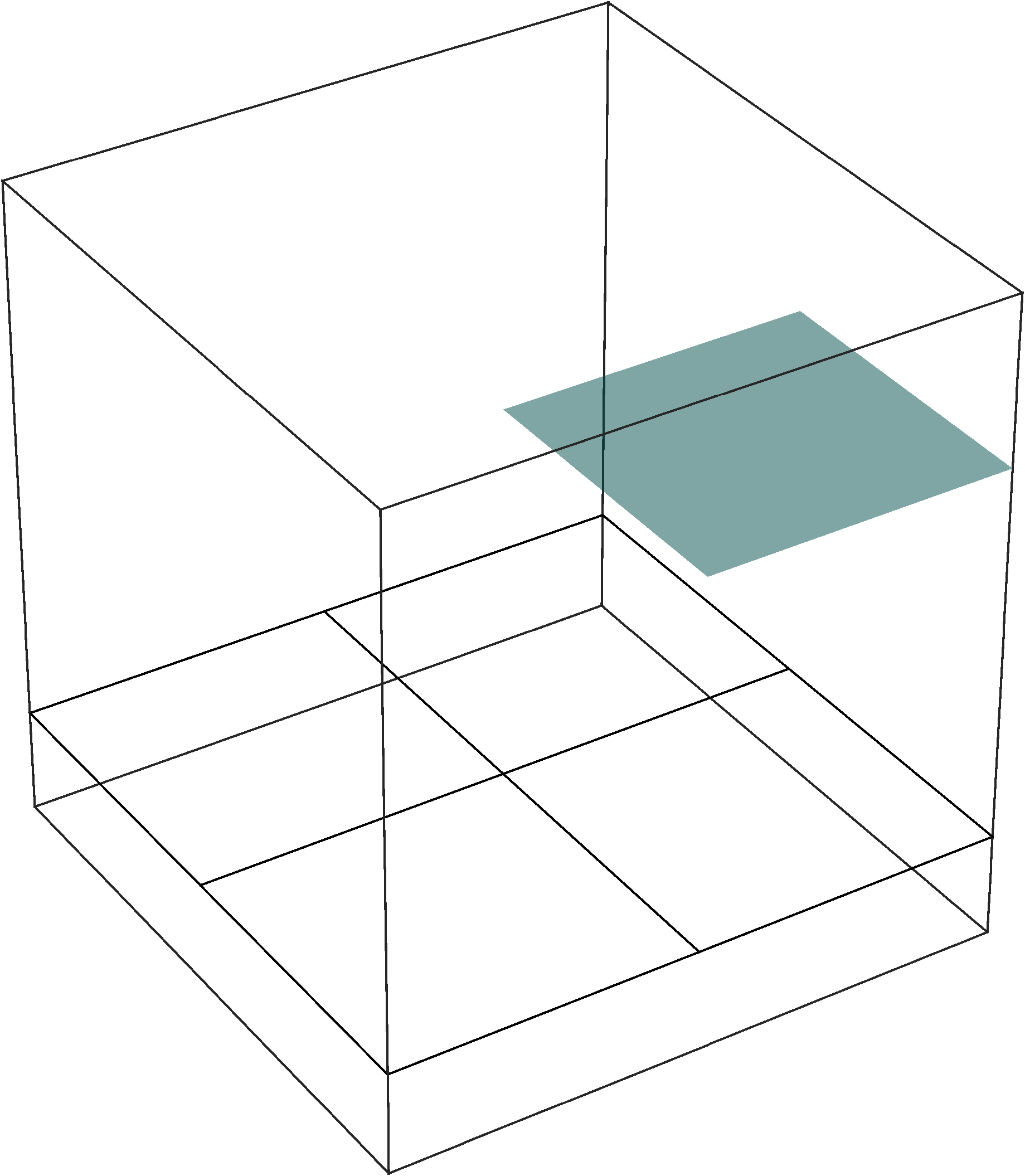
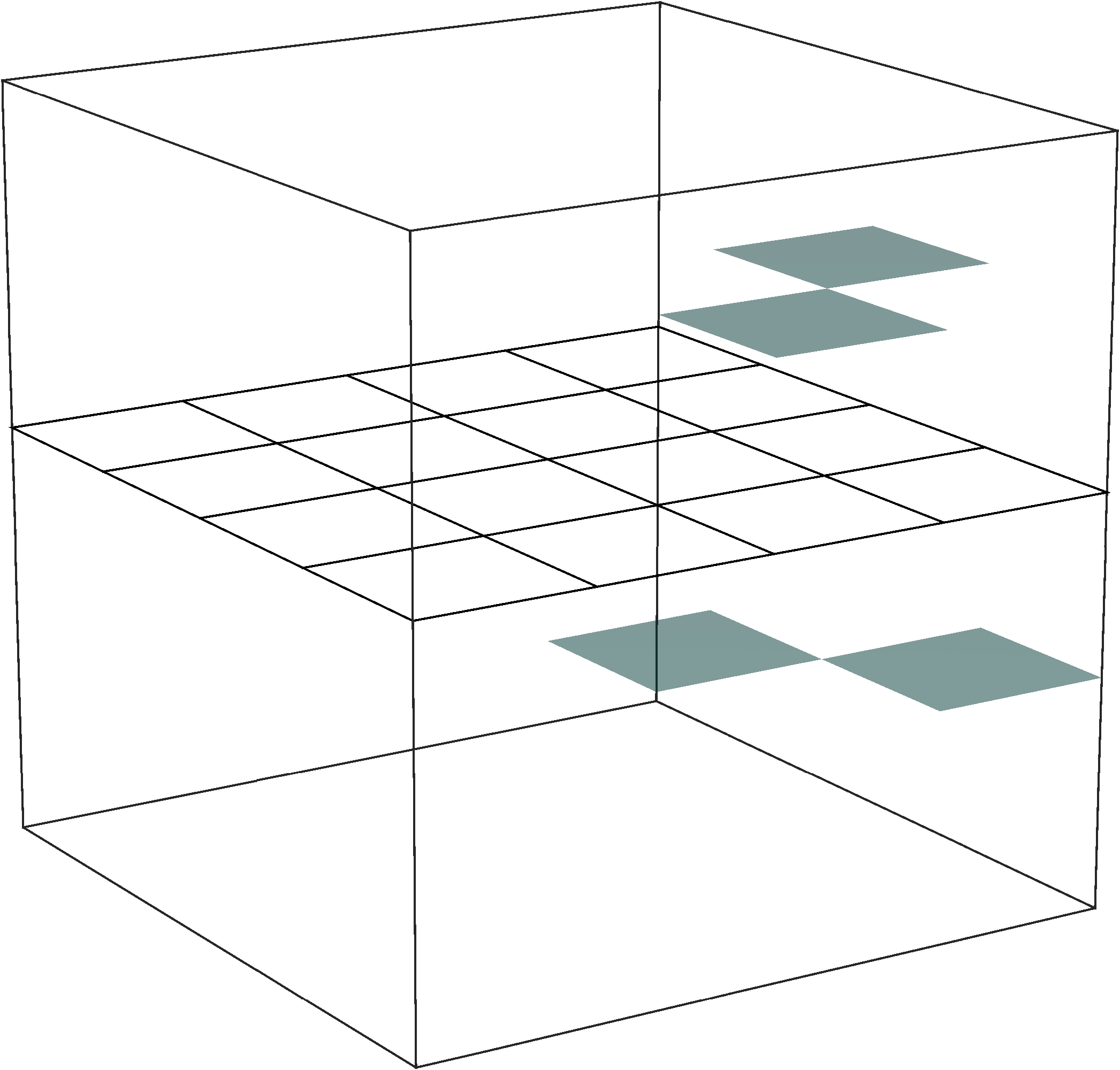
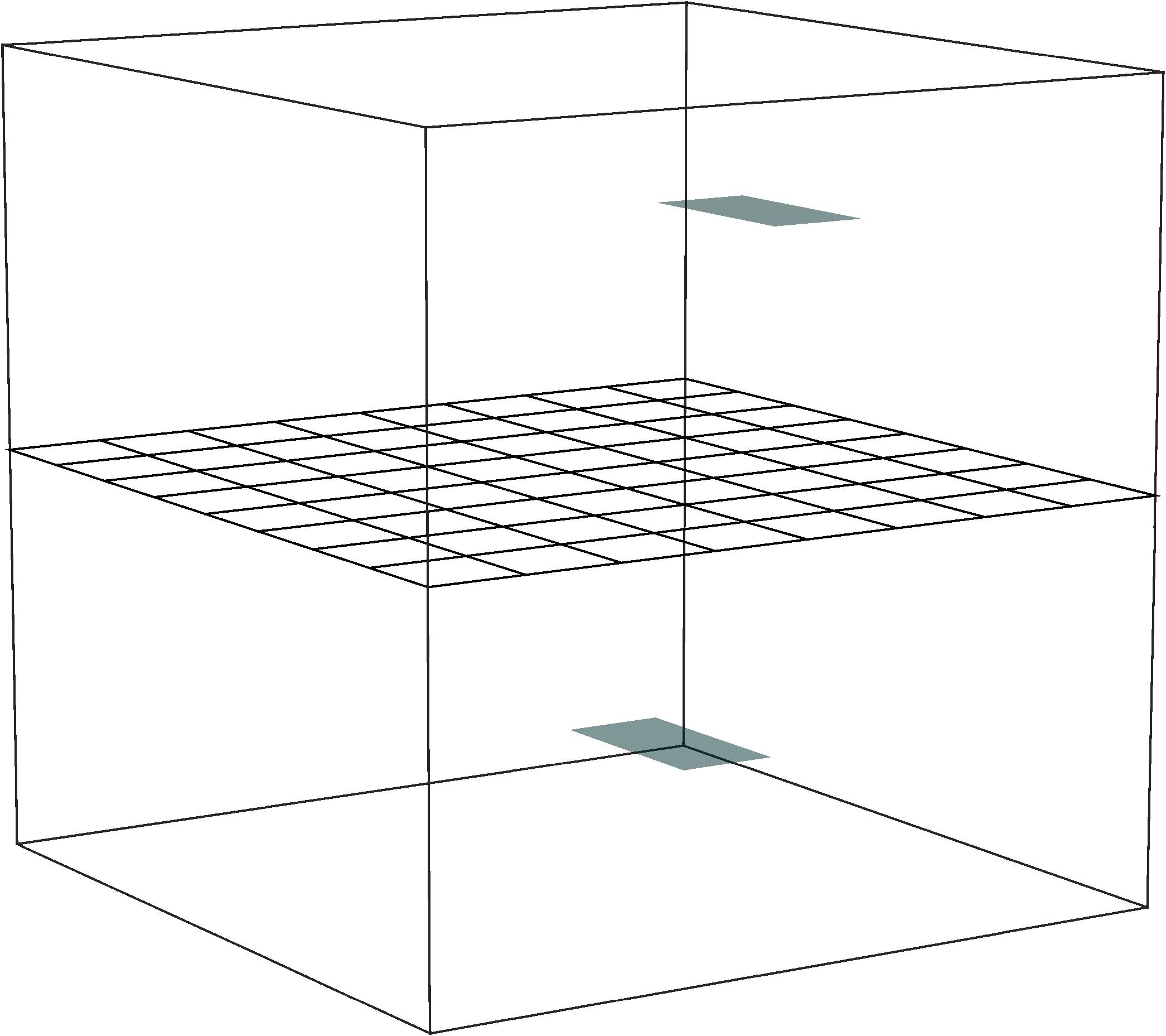
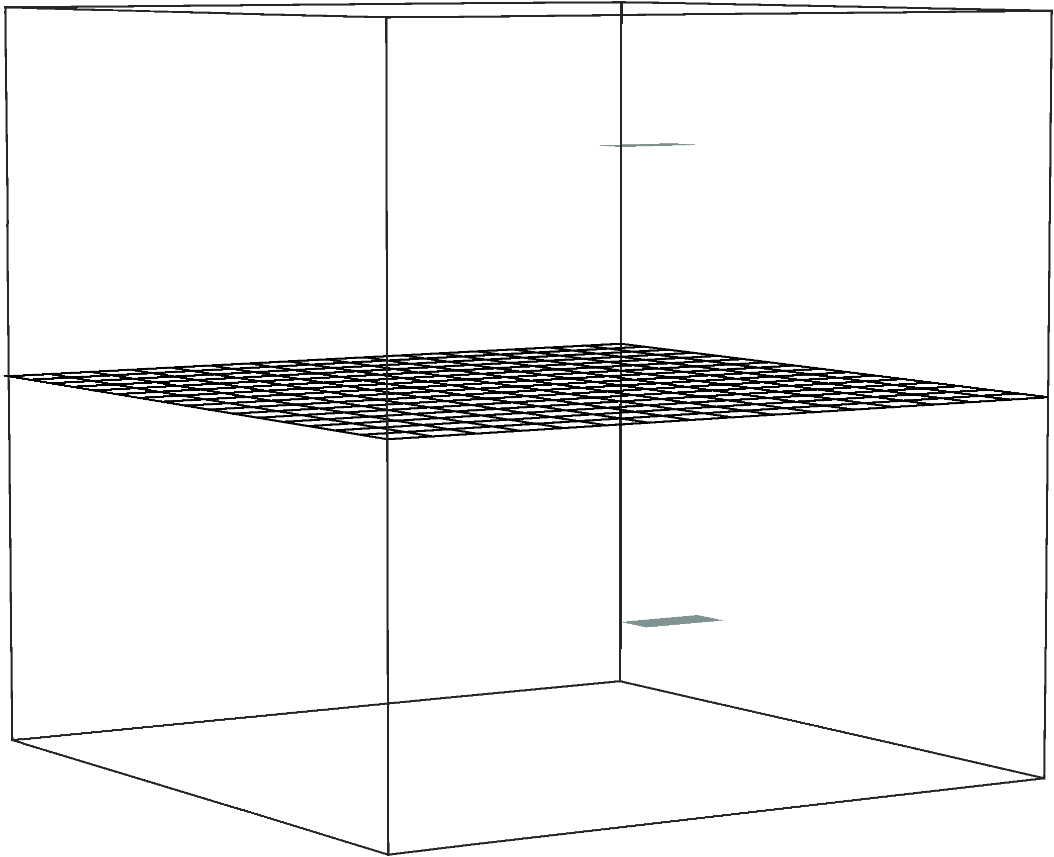
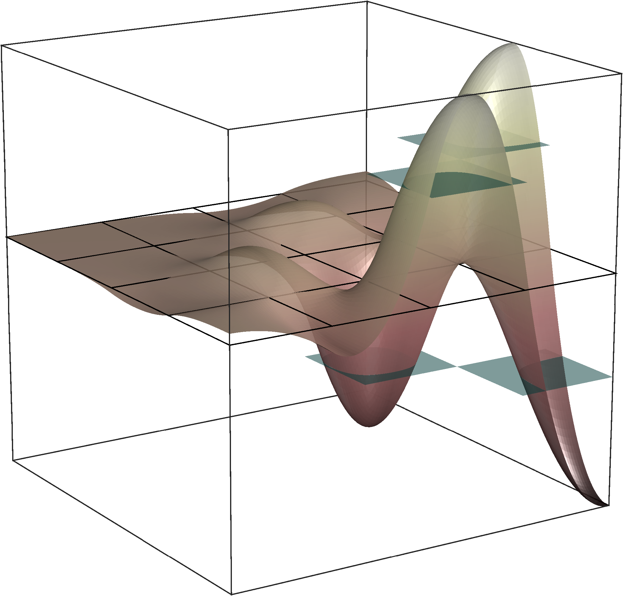
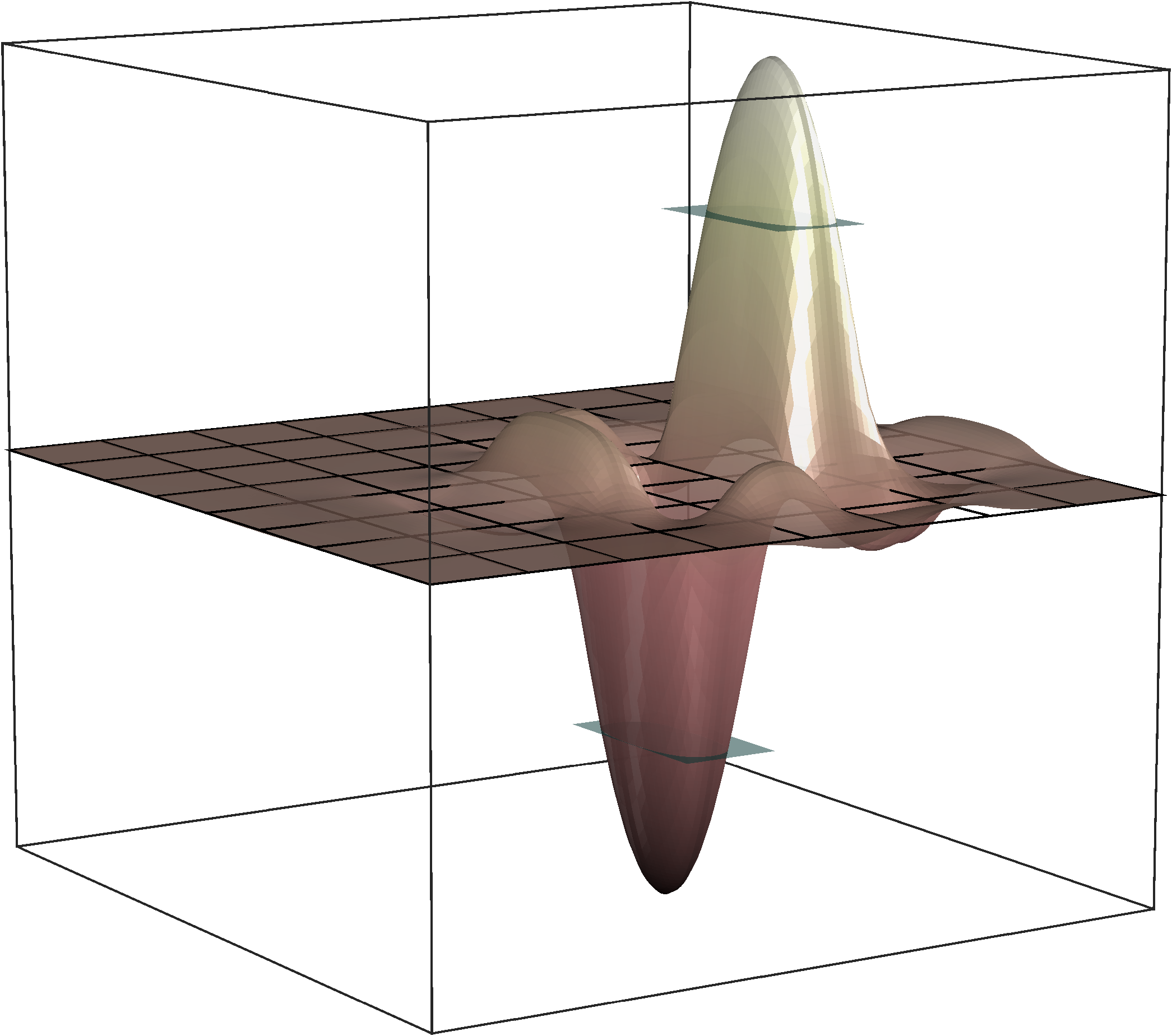
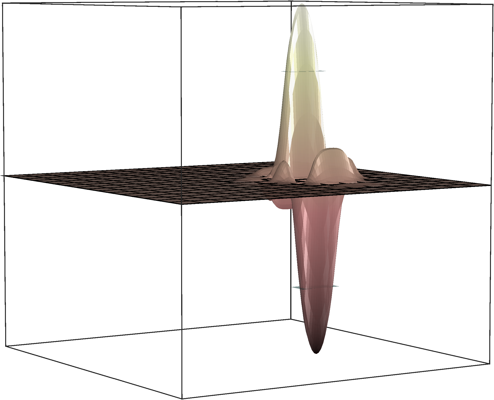
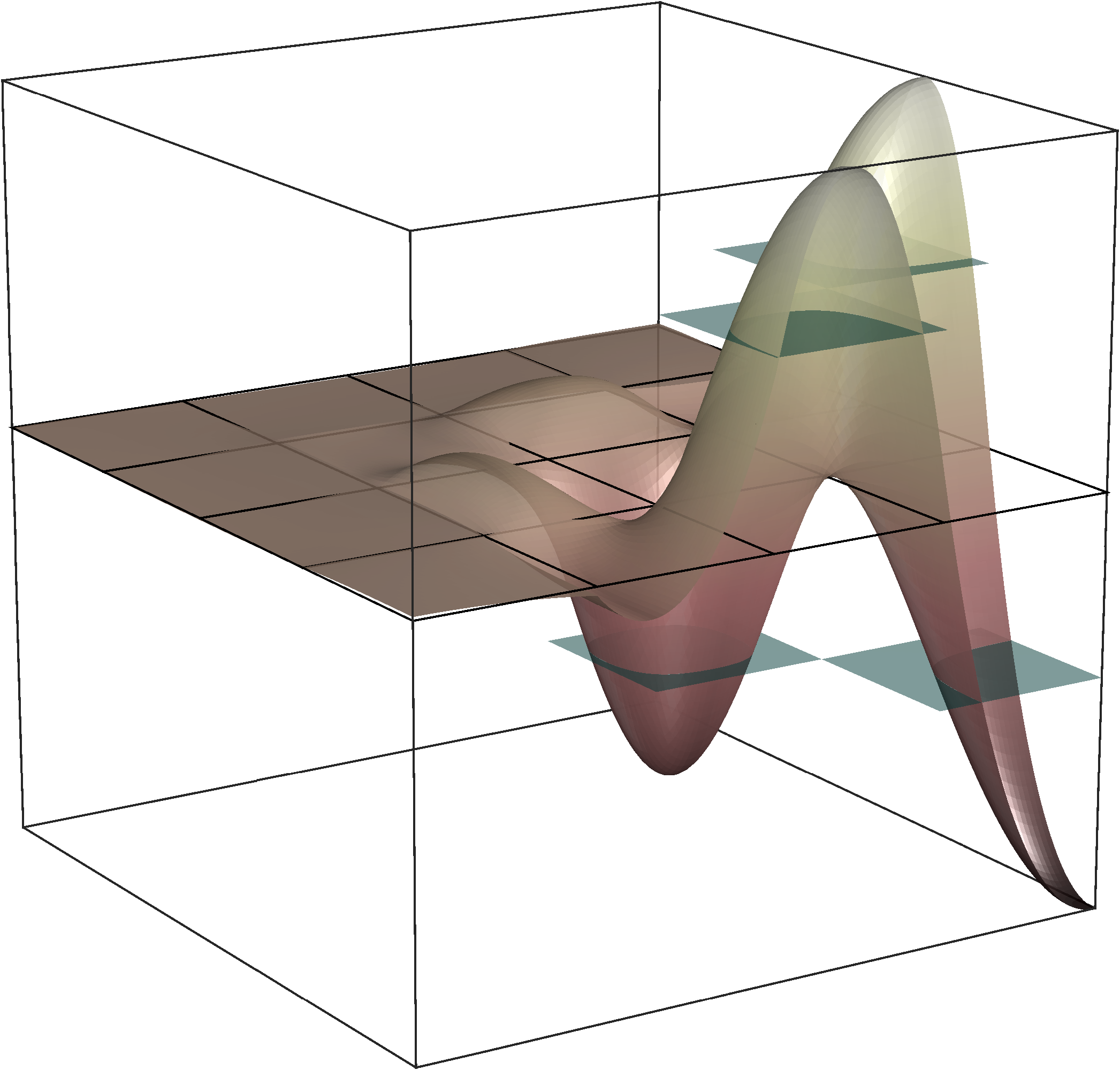
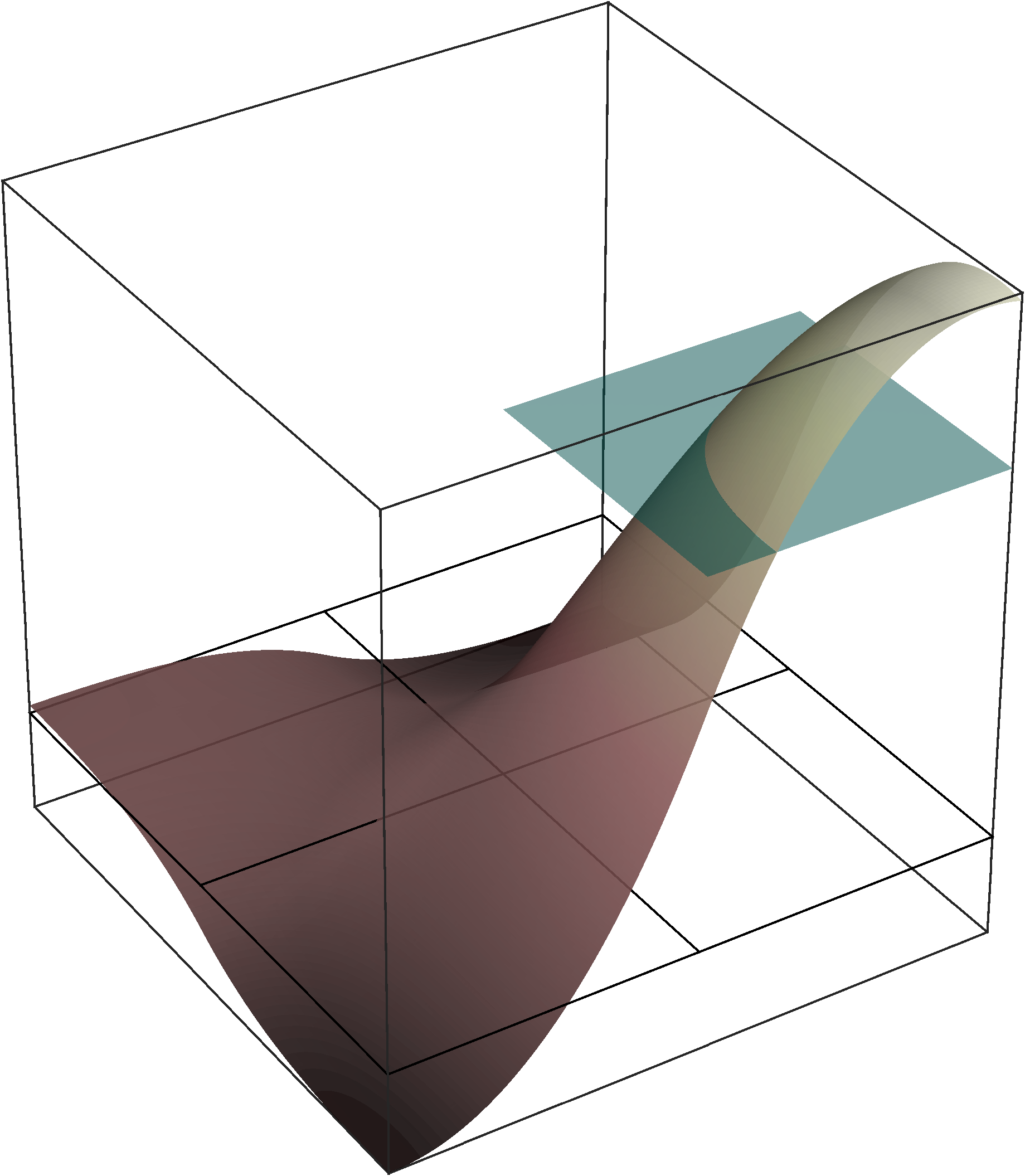
Refer to caption Refer to caption Refer to caption Refer to caption
Figure 3.1. Let 𝒯1subscript𝒯1\mathcal{T}_{1} be a Cartesian mesh of the unit square with mesh size H1=1/2subscript𝐻112H_{1}=1/2. The meshes 𝒯subscript𝒯\mathcal{T}_{\ell} for =2,3,4234\ell=2,3,4 are obtained by successive uniform refinements of 𝒯1subscript𝒯1\mathcal{T}_{1}. The pictures illustrate one (randomly chosen) Haar basis function per level.

3.2. Bubble functions

Clearly, the Haar spaces are non-conforming, i.e., 𝒱not-subset-ofsubscript𝒱\mathcal{H}_{\ell}\not\subset\mathcal{V}. For the construction of the problem-adapted hierarchical basis, we introduce conforming companions to element-wise constant functions with the same element-averages.

For =1,,L1𝐿\ell=1,...,L and all T𝒯𝑇subscript𝒯T\in\mathcal{T}_{\ell} define

bT:=b(H1x1aT,1)b(H1xdaT,d) with b(x):=6x(1x)𝟏[0,1](x)formulae-sequenceassignsubscript𝑏𝑇𝑏superscriptsubscript𝐻1subscript𝑥1subscript𝑎𝑇1𝑏superscriptsubscript𝐻1subscript𝑥𝑑subscript𝑎𝑇𝑑 with assign𝑏𝑥6𝑥1𝑥subscript101𝑥b_{T}:=b(H_{\ell}^{-1}x_{1}-a_{T,1})\cdot...\cdot b(H_{\ell}^{-1}x_{d}-a_{T,d})\quad\text{ with }\quad b(x):=6x(1-x)\mathbf{1}_{[0,1]}(x)

and aT,ksubscript𝑎𝑇𝑘a_{T,k} as above (note that 01b(x)dx=1superscriptsubscript01𝑏𝑥d𝑥1\int_{0}^{1}b(x)\,\text{d}x=1). We define the linear mapping Π~:0(𝒯)𝒱:subscript~Πsubscript0subscript𝒯𝒱\widetilde{\Pi}_{\ell}:\mathbb{Q}_{0}(\mathcal{T}_{\ell})\rightarrow\mathcal{V} uniquely by setting

Π~𝟏T:=bTforT𝒯.formulae-sequenceassignsubscript~Πsubscript1𝑇subscript𝑏𝑇for𝑇subscript𝒯\widetilde{\Pi}_{\ell}\mathbf{1}_{T}:=b_{T}\quad\text{for}\quad T\in\mathcal{T}_{\ell}.

It maps 0(𝒯)subscript0subscript𝒯\mathbb{Q}_{0}(\mathcal{T}_{\ell})-functions to conforming bubble functions with the same element averages. The operator is the right inverse of ΠsubscriptΠ\Pi_{\ell}, where Π:L2(D)0(𝒯):subscriptΠsuperscript𝐿2𝐷subscript0subscript𝒯\Pi_{\ell}:L^{2}(D)\rightarrow\mathbb{Q}_{0}(\mathcal{T}_{\ell}) denotes the L2superscript𝐿2L^{2}-orthogonal projection onto the space of element-wise constants with respect to 𝒯subscript𝒯\mathcal{T}_{\ell}. The operators ΠsubscriptΠ\Pi_{\ell} and Π~subscript~Π\widetilde{\Pi}_{\ell} satisfy for all T𝒯𝑇subscript𝒯T\in\mathcal{T}_{\ell}

(3.1) ΠvL2(T)subscriptdelimited-∥∥subscriptΠ𝑣superscript𝐿2𝑇\displaystyle{\left\lVert\Pi_{\ell}v\right\rVert}_{L^{2}(T)} vL2(T),(1Π)vL2(T)absentsubscriptdelimited-∥∥𝑣superscript𝐿2𝑇subscriptdelimited-∥∥1subscriptΠ𝑣superscript𝐿2𝑇\displaystyle\leq{\left\lVert v\right\rVert}_{L^{2}(T)},\quad\,{\left\lVert(1-\Pi_{\ell})v\right\rVert}_{L^{2}(T)} π1HvL2(T),absentsuperscript𝜋1subscript𝐻subscriptdelimited-∥∥𝑣superscript𝐿2𝑇\displaystyle\leq\pi^{-1}H_{\ell}{\left\lVert\nabla v\right\rVert}_{L^{2}(T)},
(3.2) Π~vL2(T)subscriptnormsubscript~Π𝑣superscript𝐿2𝑇\displaystyle\|\widetilde{\Pi}_{\ell}v\|_{L^{2}(T)} vL2(T),Π~vL2(T)absentsubscriptnorm𝑣superscript𝐿2𝑇subscriptnormsubscript~Π𝑣superscript𝐿2𝑇\displaystyle\leq\|v\|_{L^{2}(T)},\qquad\quad\|\nabla\widetilde{\Pi}_{\ell}v\|_{L^{2}(T)} cinvH1vL2(T),absentsubscript𝑐invsuperscriptsubscript𝐻1subscriptnorm𝑣superscript𝐿2𝑇\displaystyle\leq c_{\mathrm{inv}}H_{\ell}^{-1}\|v\|_{L^{2}(T)},

where cinv>0subscript𝑐inv0c_{\mathrm{inv}}>0 is the constant from the inverse inequality (see e.g. [8, Lemma 1.44]).

Remark 3.1 (Construction of Haar basis and bubbles).

The construction of the Haar basis and the bubbles is not restricted to Cartesian meshes. It can be performed for non-structured quadrilateral/hexahedral or simplicial meshes; see [2, 13]. If one considers tensor-product elements, higher order versions can be constructed; see [2, 27].

Remark 3.2 (Tilde notation).

Throughout the article, we write abless-than-or-similar-to𝑎𝑏a\lesssim b in short for acb𝑎𝑐𝑏a\leq cb with a constant c𝑐c independent of κ𝜅\kappa, \ell, Hsubscript𝐻H_{\ell}, L𝐿L, and m𝑚m (greater-than-or-equivalent-to\,\gtrsim is defined analogously). The notation absimilar-to-or-equals𝑎𝑏a\simeq b is used if acb𝑎𝑐𝑏a\leq cb and bca𝑏superscript𝑐𝑎b\leq c^{\prime}a with constants c𝑐c and csuperscript𝑐c^{\prime} independent of κ𝜅\kappa, \ell, Hsubscript𝐻H_{\ell}, L𝐿L, and m𝑚m.

3.3. 𝒱𝒱\mathcal{V}-stable projection

The 𝒱𝒱\mathcal{V}-stable projection introduced in the following, plays a crucial role in the construction of the localized ansatz spaces in Section 6. The construction of the operator 𝒫subscript𝒫\mathcal{P}_{\ell} is based on the quasi-interpolation operator subscript\mathcal{I}_{\ell}, from which it inherits the 𝒱𝒱\mathcal{V}-stability. The quasi-interpolation is defined as :=ΠassignsubscriptsubscriptsubscriptΠ\mathcal{I}_{\ell}:=\mathcal{E}_{\ell}\circ\Pi_{\ell}, where :0(𝒯)1(𝒯)𝒱:subscriptsubscript0subscript𝒯subscript1subscript𝒯𝒱\mathcal{E}_{\ell}\colon\mathbb{Q}_{0}(\mathcal{T}_{\ell})\to\mathbb{Q}_{1}(\mathcal{T}_{\ell})\cap\mathcal{V} (1(𝒯)subscript1subscript𝒯\mathbb{Q}_{1}(\mathcal{T}_{\ell}) is the space of element-wise tensor-product polynomials of degree up to one) denotes the nodal averaging operator, i.e., for an interior node z𝑧z, let

(v)(z):=1|T(z)|TT(z)v|T(z)assignsubscript𝑣𝑧evaluated-at1𝑇𝑧subscript𝑇𝑇𝑧𝑣𝑇𝑧(\mathcal{E}_{\ell}v)(z):=\frac{1}{|T(z)|}\sum\nolimits_{T\in T(z)}v|_{T}(z)

with T(z):={T𝒯:zT¯}assign𝑇𝑧conditional-set𝑇subscript𝒯𝑧¯𝑇T(z):=\{T\in\mathcal{T}_{\ell}:z\in\overline{T}\}. For boundary nodes, let (v)(z):=0assignsubscript𝑣𝑧0(\mathcal{E}_{\ell}v)(z):=0. Since 𝒫subscript𝒫\mathcal{P}_{\ell} should satisfy ker𝒫=kerΠkernelsubscript𝒫kernelsubscriptΠ\ker\mathcal{P}_{\ell}=\ker\Pi_{\ell}, we need to correct vsubscript𝑣\mathcal{I}_{\ell}v such that element averages of v𝑣v on 𝒯subscript𝒯\mathcal{T}_{\ell} are preserved:

(3.3) 𝒫v:=v+T𝒯TvvdxbT.assignsubscript𝒫𝑣subscript𝑣subscript𝑇subscript𝒯subscript𝑇𝑣subscript𝑣d𝑥subscript𝑏𝑇\mathcal{P}_{\ell}v:=\mathcal{I}_{\ell}v+\sum_{T\in\mathcal{T}_{\ell}}\int_{T}v-\mathcal{I}_{\ell}v\,\text{d}x\,b_{T}.

The following stability and approximation properties are shown in [1] and are based on classical finite element theory [6, 9]. For any v𝒱𝑣𝒱v\in\mathcal{V}

(3.4) 𝒫vL2(T)vL2(N1(T)),𝒫vL2(T)vL2(N1(T)),(1𝒫)vL2(T)HvL2(N1(T)).formulae-sequenceless-than-or-similar-tosubscriptdelimited-∥∥subscript𝒫𝑣superscript𝐿2𝑇subscriptdelimited-∥∥𝑣superscript𝐿2superscriptsubscript𝑁1𝑇formulae-sequenceless-than-or-similar-tosubscriptdelimited-∥∥subscript𝒫𝑣superscript𝐿2𝑇subscriptdelimited-∥∥𝑣superscript𝐿2superscriptsubscript𝑁1𝑇less-than-or-similar-tosubscriptdelimited-∥∥1subscript𝒫𝑣superscript𝐿2𝑇subscript𝐻subscriptdelimited-∥∥𝑣superscript𝐿2superscriptsubscript𝑁1𝑇\displaystyle\begin{split}\|\mathcal{P}_{\ell}v\|_{L^{2}(T)}&\lesssim\|v\|_{L^{2}(N_{\ell}^{1}(T))},\\ \|\nabla\mathcal{P}_{\ell}v\|_{L^{2}(T)}&\lesssim\|\nabla v\|_{L^{2}(N_{\ell}^{1}(T))},\\ \|(1-\mathcal{P}_{\ell})v\|_{L^{2}(T)}&\lesssim H_{\ell}\|\nabla v\|_{L^{2}(N_{\ell}^{1}(T))}.\end{split}

4. Block-diagonal multi-resolution decomposition

In this section, we introduce a hierarchical multi-resolution Petrov-Galerkin method in order to discretize (2.3). In contrast to [34, 13], where only symmetric and elliptic problems are considered, we need two different sets of bases for trial and test spaces. This is due to the lack of hermiticity of the Helmholtz problem.

We propose a special choice of bases, which block-diagonalizes the (discretized) operator, see [13]. Each basis function is assigned to (exactly) one Haar basis function ϕ,jsubscriptitalic-ϕ𝑗\phi_{\ell,j}. Since the basis functions, in general, have global support (c.f. Figure 4.1), the ideal method is not suited for practical purposes. A practical method is derived in Section 6 by localizing the basis functions to element patches. This procedure is justified by the exponential decay of the basis functions (Section 5).

4.1. Correction operators

The concept of correction operators is key in the LOD framework. In the multi-level context, one considers correction operators on every level projecting onto 𝒲:=kerΠassignsubscript𝒲kersubscriptΠ\mathcal{W}_{\ell}:=\mathrm{ker}\,\Pi_{\ell}. The spaces 𝒲subscript𝒲\mathcal{W}_{\ell} can be interpreted as (infinite-dimensional) subspaces of 𝒱𝒱\mathcal{V} consisting of functions oscillating on length scales smaller than Hsubscript𝐻H_{\ell}. The fine scale spaces are nested, i.e., 𝒲1𝒲Lsuperset-ofsubscript𝒲1superset-ofsubscript𝒲𝐿\mathcal{W}_{1}\supset...\supset\mathcal{W}_{L}.

For the correction operators to be well-defined, we need to assume a minimal resolution condition.

Assumption 4.1 (Resolution condition).

Given the wave number κ𝜅\kappa, we assume that the mesh size H1subscript𝐻1H_{1} of 𝒯1subscript𝒯1\mathcal{T}_{1} satisfies

H1κπ2.subscript𝐻1𝜅𝜋2H_{1}\kappa\leq\frac{\pi}{\sqrt{2}}.

Due to the lack of hermiticity, we need to define for =1,,L1𝐿\ell=1,...,L the two correction operators 𝒞subscript𝒞\mathcal{C}_{\ell} and 𝒞superscriptsubscript𝒞\mathcal{C}_{\ell}^{*} as

(4.1) 𝒞:𝒱𝒲,a(𝒞v,w)=a(v,w)for all w𝒲,𝒞:𝒱𝒲,a(w,𝒞v)=a(w,v)for all w𝒲.:subscript𝒞formulae-sequence𝒱subscript𝒲formulae-sequence𝑎subscript𝒞𝑣𝑤𝑎𝑣𝑤for all 𝑤subscript𝒲superscriptsubscript𝒞:formulae-sequence𝒱subscript𝒲formulae-sequence𝑎𝑤superscriptsubscript𝒞𝑣𝑎𝑤𝑣for all 𝑤subscript𝒲\displaystyle\begin{split}\mathcal{C}_{\ell}:\mathcal{V}\rightarrow\mathcal{W}_{\ell},\ a(\mathcal{C}_{\ell}v,w)&=a(v,w)\quad\text{for all }w\in\mathcal{W}_{\ell},\\ \mathcal{C}_{\ell}^{*}:\mathcal{V}\rightarrow\mathcal{W}_{\ell},\ a(w,\mathcal{C}_{\ell}^{*}v)&=a(w,v)\quad\text{for all }w\in\mathcal{W}_{\ell}.\end{split}

One can show the identity 𝒞v=𝒞v¯¯superscriptsubscript𝒞𝑣¯subscript𝒞¯𝑣\mathcal{C}_{\ell}^{*}v=\overline{\mathcal{C}_{\ell}\overline{v}} for all v𝒱𝑣𝒱v\in\mathcal{V}. The well-posedness of 𝒞subscript𝒞\mathcal{C}_{\ell} and 𝒞superscriptsubscript𝒞\mathcal{C}_{\ell}^{*} follows from the resolution condition.

Lemma 4.2 (Well-posedness of corrector problems).

Under Assumption 4.1, a𝑎a is coercive on 𝒲1×𝒲1subscript𝒲1subscript𝒲1\mathcal{W}_{1}\times\mathcal{W}_{1}, i.e.,

a(w,w)12wL2(D).𝑎𝑤𝑤12subscriptnorm𝑤superscript𝐿2𝐷\mathfrak{R}a(w,w)\geq\frac{1}{2}\|\nabla w\|_{L^{2}(D)}.

Additionally, the norms 𝒱(D)\|\cdot\|_{\mathcal{V}(D)} and L2(D)\|\nabla\cdot\|_{L^{2}(D)} are equivalent on 𝒲1subscript𝒲1\mathcal{W}_{1} independently of κ𝜅\kappa.

Proof.

a𝑎a is coercive on 𝒲1×𝒲1subscript𝒲1subscript𝒲1\mathcal{W}_{1}\times\mathcal{W}_{1}, since

a(w,w)𝑎𝑤𝑤\displaystyle\mathfrak{R}a(w,w) wL2(D)2κ2wL2(D)=wL2(D)2κ2(1Π1)wL2(D)2absentsuperscriptsubscriptdelimited-∥∥𝑤superscript𝐿2𝐷2superscript𝜅2subscriptdelimited-∥∥𝑤superscript𝐿2𝐷superscriptsubscriptdelimited-∥∥𝑤superscript𝐿2𝐷2superscript𝜅2superscriptsubscriptdelimited-∥∥1subscriptΠ1𝑤superscript𝐿2𝐷2\displaystyle\geq{\left\lVert\nabla w\right\rVert}_{L^{2}(D)}^{2}-\kappa^{2}{\left\lVert w\right\rVert}_{L^{2}(D)}={\left\lVert\nabla w\right\rVert}_{L^{2}(D)}^{2}-\kappa^{2}{\left\lVert(1-\Pi_{1})w\right\rVert}_{L^{2}(D)}^{2}
wL2(D)2π2(H1κ)2wL2(D)212wL2(D)2absentsuperscriptsubscriptdelimited-∥∥𝑤superscript𝐿2𝐷2superscript𝜋2superscriptsubscript𝐻1𝜅2superscriptsubscriptdelimited-∥∥𝑤superscript𝐿2𝐷212superscriptsubscriptdelimited-∥∥𝑤superscript𝐿2𝐷2\displaystyle\geq{\left\lVert\nabla w\right\rVert}_{L^{2}(D)}^{2}-\pi^{-2}(H_{1}\kappa)^{2}{\left\lVert\nabla w\right\rVert}_{L^{2}(D)}^{2}\geq\frac{1}{2}{\left\lVert\nabla w\right\rVert}_{L^{2}(D)}^{2}

using Assumption 4.1. The norm equivalence of L2(D){\left\lVert\nabla\cdot\right\rVert}_{L^{2}(D)} and 𝒱(D)subscriptdelimited-∥∥𝒱𝐷{\left\lVert\cdot\right\rVert}_{\mathcal{V}(D)} follows from

wL2(D)2w𝒱(D)2=wL2(D)2+κ2(1Π1)wL2(D)232wL2(D)2superscriptsubscriptdelimited-∥∥𝑤superscript𝐿2𝐷2superscriptsubscriptdelimited-∥∥𝑤𝒱𝐷2superscriptsubscriptdelimited-∥∥𝑤superscript𝐿2𝐷2superscript𝜅2superscriptsubscriptdelimited-∥∥1subscriptΠ1𝑤superscript𝐿2𝐷232superscriptsubscriptdelimited-∥∥𝑤superscript𝐿2𝐷2{\left\lVert\nabla w\right\rVert}_{L^{2}(D)}^{2}\leq{\left\lVert w\right\rVert}_{\mathcal{V}(D)}^{2}={\left\lVert\nabla w\right\rVert}_{L^{2}(D)}^{2}+\kappa^{2}{\left\lVert(1-\Pi_{1})w\right\rVert}_{L^{2}(D)}^{2}\leq\frac{3}{2}{\left\lVert\nabla w\right\rVert}_{L^{2}(D)}^{2}

using again the same assumption.

Remark 4.3 (Well-posedness of correctors).

The well-posedness of (4.1) can be concluded using the Lax–Milgram lemma using the coercivity of a𝑎a on 𝒲1×𝒲1subscript𝒲1subscript𝒲1\mathcal{W}_{1}\times\mathcal{W}_{1} shown in Lemma 4.2 and the continuity of a𝑎a (2.4). In general, it holds that the complementary projection and the projection itself have the same operator norms (c.f. [43]). Thus, we get boundedness of 𝒞subscript𝒞\mathcal{C}_{\ell}, 𝒞superscriptsubscript𝒞\mathcal{C}_{\ell}^{*}, 1𝒞1subscript𝒞1-\mathcal{C}_{\ell}, and 1𝒞1superscriptsubscript𝒞1-\mathcal{C}_{\ell}^{*} all with the same constants.

4.2. Trial and test spaces

Using the correction operators, we can define the hierarchical multi-resolution trial and test spaces of the method. For levels =1,,L1𝐿\ell=1,...,L, let

(4.2) Φ~:=span{(1𝒞){Π~ϕ,j,j=1,,N}},Ψ~:=span{(1𝒞){Π~ϕ,j,j=1,,N}}.\displaystyle\begin{split}{\widetilde{\Phi}}_{\ell}&:=\mathrm{span}\big{\{}(1-\mathcal{C}_{\ell})\{\widetilde{\Pi}_{\ell}\phi_{\ell,j},j=1,...,N_{\ell}\}\big{\}},\\ {\widetilde{\Psi}}_{\ell}&:=\mathrm{span}\big{\{}(1-\mathcal{C}^{*}_{\ell})\{\widetilde{\Pi}_{\ell}\phi_{\ell,j},j=1,...,N_{\ell}\}\big{\}}.\end{split}

The canonical bases of Φ~subscript~Φ\widetilde{\Phi}_{\ell} and Ψ~subscript~Ψ\widetilde{\Psi}_{\ell} are given by {b,j:=(1𝒞)Π~ϕ,j,j=1,,N}formulae-sequenceassignsubscript𝑏𝑗1subscript𝒞subscript~Πsubscriptitalic-ϕ𝑗𝑗1subscript𝑁\{b_{\ell,j}:=(1-\mathcal{C}_{\ell})\widetilde{\Pi}_{\ell}\phi_{\ell,j},j=1,...,N_{\ell}\} and {b,j:=(1𝒞)Π~ϕ,j,j=1,,N}formulae-sequenceassignsuperscriptsubscript𝑏𝑗1superscriptsubscript𝒞subscript~Πsubscriptitalic-ϕ𝑗𝑗1subscript𝑁\{b_{\ell,j}^{*}:=(1-\mathcal{C}_{\ell}^{*})\widetilde{\Pi}_{\ell}\phi_{\ell,j},j=1,...,N_{\ell}\}, respectively.

Let us define the spaces 𝒰~:=Φ~1Φ~Lassign~𝒰direct-sumsubscript~Φ1subscript~Φ𝐿\widetilde{\mathcal{U}}:=\widetilde{\Phi}_{1}\oplus...\oplus\widetilde{\Phi}_{L} and 𝒱~:=Ψ~1Ψ~Lassign~𝒱direct-sumsubscript~Ψ1subscript~Ψ𝐿\widetilde{\mathcal{V}}:=\widetilde{\Psi}_{1}\oplus...\oplus\widetilde{\Psi}_{L}.

Remark 4.4 (Conforming version of subscript\mathcal{H}_{\ell}).

Note that Π~subscript~Πsubscript\widetilde{\Pi}_{\ell}\mathcal{H}_{\ell} is a conformal version of subscript\mathcal{H}_{\ell}. It holds that Π~ϕ,jsubscript~Πsubscriptitalic-ϕ𝑗\widetilde{\Pi}_{\ell}\phi_{\ell,j} and ϕ,jsubscriptitalic-ϕ𝑗\phi_{\ell,j} have the same element-averages on 𝒯subscript𝒯\mathcal{T}_{\ell}. The precise choice of Π~subscript~Π\widetilde{\Pi}_{\ell} is not important as long as its image is conforming, it preserves element-averages, and (3.2) holds.
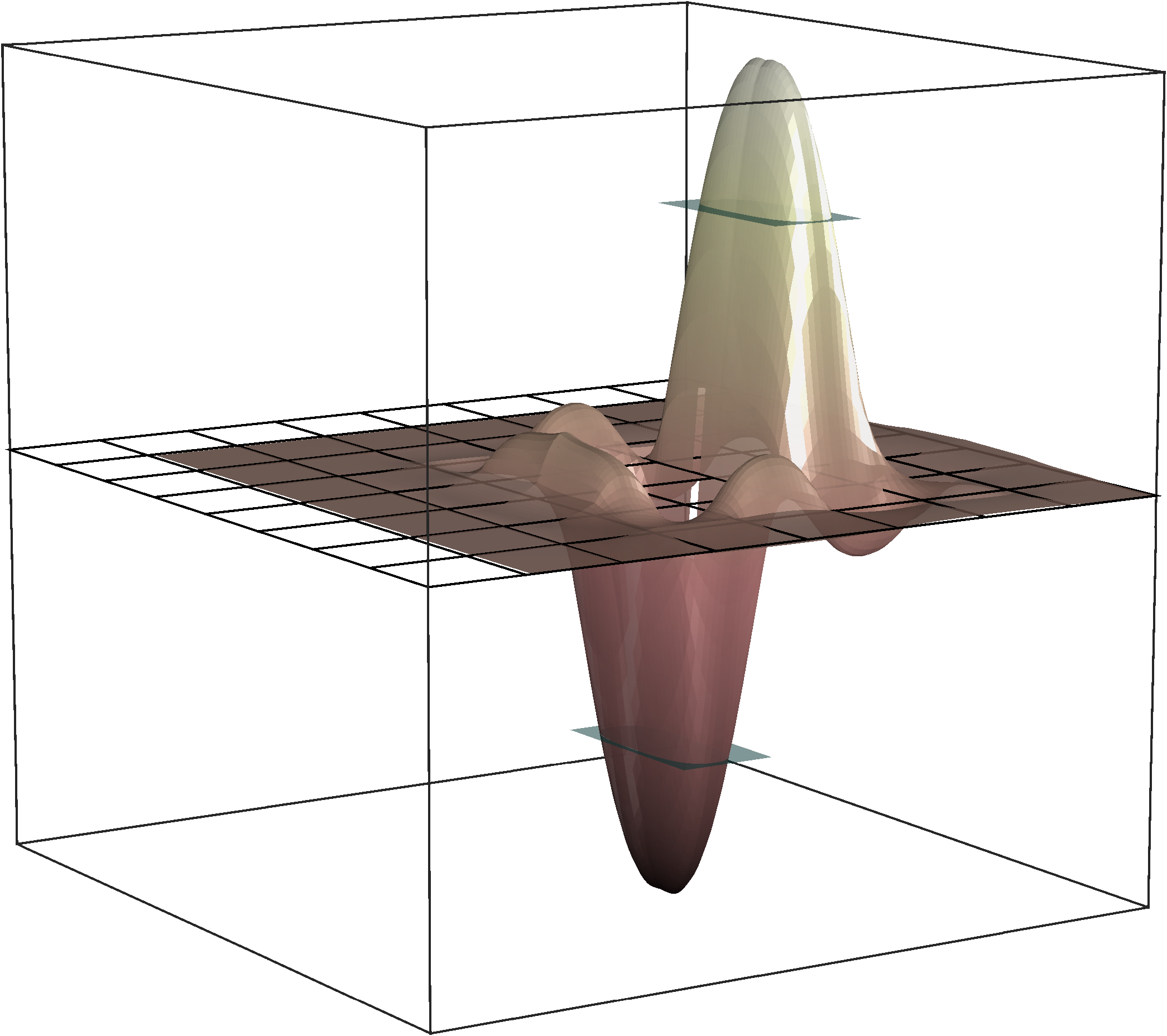
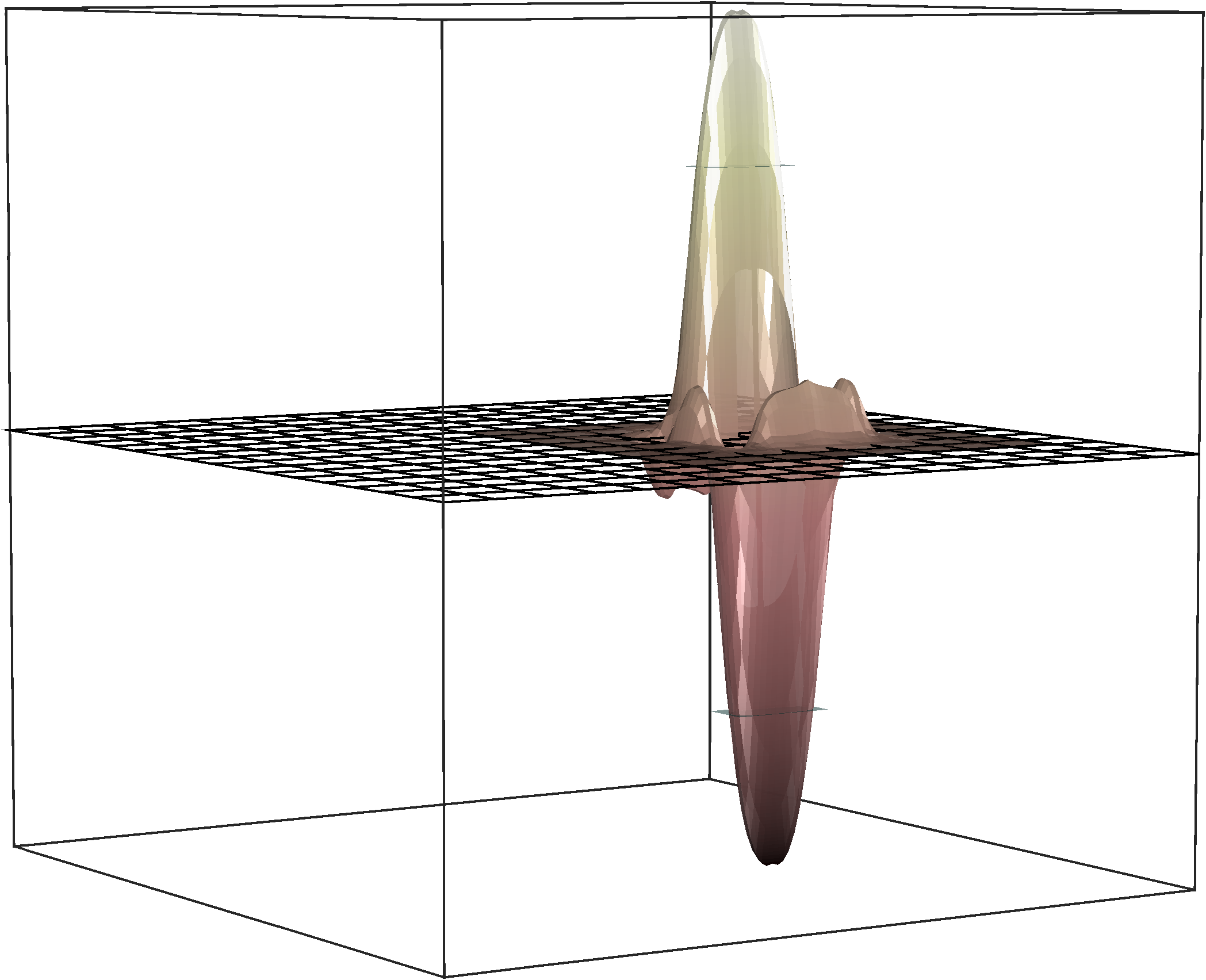
Refer to caption Refer to caption Refer to caption Refer to caption
Figure 4.1. Let the mesh hierarchy be as for Figure 3.1. The pictures show the real part of one (randomly chosen) basis function b,jsubscript𝑏𝑗b_{\ell,j} per level. The corresponding Haar basis functions ϕ,jsubscriptitalic-ϕ𝑗\phi_{\ell,j} are indicated in green.
Remark 4.5 (Relationship to [1]).

In [1], the LOD method is introduced using a very general framework. So called ’quantities of interest’ determine the precise method. Using the element-averages on the mesh 𝒯Lsubscript𝒯𝐿\mathcal{T}_{L} as quantities of interest, we can prove the relationships

(1𝒞L)𝒱=Φ~1Φ~L and (1𝒞L)𝒱=Ψ~1Ψ~L,formulae-sequence1subscript𝒞𝐿𝒱direct-sumsubscript~Φ1subscript~Φ𝐿 and 1subscriptsuperscript𝒞𝐿𝒱direct-sumsubscript~Ψ1subscript~Ψ𝐿(1-\mathcal{C}_{L})\mathcal{V}=\widetilde{\Phi}_{1}\oplus...\oplus\widetilde{\Phi}_{L}\quad\text{ and }\quad(1-\mathcal{C}^{*}_{L})\mathcal{V}=\widetilde{\Psi}_{1}\oplus...\oplus\widetilde{\Psi}_{L},

where (1𝒞L)𝒱1subscript𝒞𝐿𝒱(1-\mathcal{C}_{L})\mathcal{V} and (1𝒞L)𝒱1superscriptsubscript𝒞𝐿𝒱(1-\mathcal{C}_{L}^{*})\mathcal{V} are the trial and test spaces from [1], respectively. This relationship, in general, is not true for the practical method derived in Section 6.

From Definition (4.1), one can deduce for k,{1,,L}𝑘1𝐿k,\ell\in\{1,...,L\} with k𝑘k\leq\ell the ’orthogonality’ (a𝑎a is not an inner-product) relations

(4.3) a(Φ~k,𝒲)=0 and a(𝒲,Ψ~k)=0.formulae-sequence𝑎subscript~Φ𝑘subscript𝒲0 and 𝑎subscript𝒲subscript~Ψ𝑘0a(\widetilde{\Phi}_{k},\mathcal{W}_{\ell})=0\quad\text{ and }\quad a(\mathcal{W}_{\ell},\widetilde{\Psi}_{k})=0.

The single-level method discretizing (2.3) is based on the trial-test pairing (𝒰~,𝒱~)~𝒰~𝒱(\widetilde{\mathcal{U}},\widetilde{\mathcal{V}}) and seeks u~𝒰~~𝑢~𝒰\tilde{u}\in\widetilde{\mathcal{U}}, such that for all v~𝒱~~𝑣~𝒱\tilde{v}\in\widetilde{\mathcal{V}}

(4.4) a(u~,v~)=(f,v~)L2(D).𝑎~𝑢~𝑣subscript𝑓~𝑣superscript𝐿2𝐷a(\tilde{u},\tilde{v})={\left(f\,,\,\tilde{v}\right)}_{L^{2}(D)}.

Henceforth, we refer to (4.4) as ideal method, since this method only has theoretical purposes and cannot be applied in practice; see Section 6.

4.3. Stability and accuracy of ideal method

Since (4.4) coincides with the ideal method from [37], also the stability result and convergence results are the same.

Lemma 4.6 (Stability of ideal method).

Let Assumption 4.1 be satisfied. Then the trial space 𝒰~~𝒰\widetilde{\mathcal{U}} and the test space 𝒱~~𝒱\widetilde{\mathcal{V}} satisfy the inf-sup condition

0<α(2)infu~𝒰~supv~𝒱~a(u~,v~)u~𝒱(D)v~𝒱(D)0superscript𝛼2subscriptinfimum~𝑢~𝒰subscriptsupremum~𝑣~𝒱𝑎~𝑢~𝑣subscriptdelimited-∥∥~𝑢𝒱𝐷subscriptdelimited-∥∥~𝑣𝒱𝐷0<\alpha^{(2)}\leq\inf_{\tilde{u}\in\widetilde{\mathcal{U}}}\sup_{\tilde{v}\in\widetilde{\mathcal{V}}}\frac{\mathfrak{R}a(\tilde{u},\tilde{v})}{{\left\lVert\tilde{u}\right\rVert}_{\mathcal{V}(D)}{\left\lVert\tilde{v}\right\rVert}_{\mathcal{V}(D)}}

with α(2)(cstab(κ)κ)1similar-to-or-equalssuperscript𝛼2superscriptsubscript𝑐stab𝜅𝜅1\alpha^{(2)}\simeq(c_{\mathrm{stab}}(\kappa)\kappa)^{-1}.

Proof.

For the proof, see Appendix A. ∎

Lemma 4.7 (Accuracy of ideal method).

Let u𝒱𝑢𝒱u\in\mathcal{V} be the solution of (2.3) for the right-hand side f𝑓f. If Assumption 4.1 is satisfied, then u~=(1𝒞L)u𝒰~~𝑢1subscript𝒞𝐿𝑢~𝒰\tilde{u}=(1-\mathcal{C}_{L})u\in\widetilde{\mathcal{U}} is the unique solution of (4.4), that is, the Petrov-Galerkin approximation of u𝑢u in the subspace 𝒰~~𝒰\widetilde{\mathcal{U}} with respect to the test space 𝒱~~𝒱\widetilde{\mathcal{V}}. Moreover, there is a constant c𝑐c independent of κ,HL𝜅subscript𝐻𝐿\kappa,H_{L} and L𝐿L such that for any fHs(D)𝑓superscript𝐻𝑠𝐷f\in H^{s}(D), s[0,1]𝑠01s\in[0,1]

uu~𝒱(D)cHL1+sfHs(D).subscriptdelimited-∥∥𝑢~𝑢𝒱𝐷𝑐superscriptsubscript𝐻𝐿1𝑠subscriptnorm𝑓superscript𝐻𝑠𝐷{\left\lVert u-\tilde{u}\right\rVert}_{\mathcal{V}(D)}\leq cH_{L}^{1+s}\|f\|_{H^{s}(D)}.
Proof.

For the proof, see Appendix A. ∎

4.4. Block-diagonalization

The special choice of the hierarchy of bases (4.2) decouples the equations on every level; see also [34, 13].

Lemma 4.8 (’Orthogonality’ of levels).

Let Assumption 4.1 be satisfied. Consider k,{1,,L}𝑘1𝐿k,\ell\in\{1,...,L\}, with k𝑘k\neq\ell. Then it holds for all φ~kΦ~k,ψ~Ψ~formulae-sequencesubscript~𝜑𝑘subscript~Φ𝑘subscript~𝜓subscript~Ψ\tilde{\varphi}_{k}\in\widetilde{\Phi}_{k},\tilde{\psi}_{\ell}\in\widetilde{\Psi}_{\ell}

a(φ~k,ψ~)=0.𝑎subscript~𝜑𝑘subscript~𝜓0a(\tilde{\varphi}_{k},\tilde{\psi}_{\ell})=0.
Proof.

First suppose that k>𝑘k>\ell. We show that Φ~k𝒲subscript~Φ𝑘subscript𝒲\widetilde{\Phi}_{k}\subset\mathcal{W}_{\ell}. Let Φ~kφ~k=(1𝒞k)Π~kϕkcontainssubscript~Φ𝑘subscript~𝜑𝑘1subscript𝒞𝑘subscript~Π𝑘subscriptitalic-ϕ𝑘\widetilde{\Phi}_{k}\ni\tilde{\varphi}_{k}=(1-\mathcal{C}_{k})\widetilde{\Pi}_{k}\phi_{k} with ϕkspan{k}subscriptitalic-ϕ𝑘spansubscript𝑘\phi_{k}\in\mathrm{span}\{\mathcal{H}_{k}\} be arbitrary, then

Π(1𝒞k)Π~kϕk=ΠΠk(1𝒞k)Π~kϕk=Πϕk=0.subscriptΠ1subscript𝒞𝑘subscript~Π𝑘subscriptitalic-ϕ𝑘subscriptΠsubscriptΠ𝑘1subscript𝒞𝑘subscript~Π𝑘subscriptitalic-ϕ𝑘subscriptΠsubscriptitalic-ϕ𝑘0\Pi_{\ell}(1-\mathcal{C}_{k})\widetilde{\Pi}_{k}\phi_{k}=\Pi_{\ell}\Pi_{k}(1-\mathcal{C}_{k})\widetilde{\Pi}_{k}\phi_{k}=\Pi_{\ell}\phi_{k}=0.

Together with (4.3), this implies the assertion. If k<𝑘k<\ell, one can similarly show that Ψ~𝒲ksubscript~Ψsubscript𝒲𝑘\widetilde{\Psi}_{\ell}\subset\mathcal{W}_{k}, which again yields the assertion. ∎

Corollary 4.9.

Let Assumption 4.1 be satisfied, then for {2,,L}2𝐿\ell\in\{2,...,L\} it holds that

Φ~𝒲1𝒲1, and Ψ~𝒲1𝒲1.formulae-sequencesubscript~Φsubscript𝒲1subscript𝒲1 and subscript~Ψsubscript𝒲1subscript𝒲1\widetilde{\Phi}_{\ell}\subset\mathcal{W}_{\ell-1}\subset\mathcal{W}_{1},\quad\text{ and }\quad\widetilde{\Psi}_{\ell}\subset\mathcal{W}_{\ell-1}\subset\mathcal{W}_{1}.
Proof.

This is an immediate consequence of the proof of Lemma 4.8. ∎

Using Lemma 4.8, we can rewrite (4.4) into decoupled Petrov-Galerkin problems on every level, which seek φ~Φ~subscript~𝜑subscript~Φ\tilde{\varphi}_{\ell}\in\widetilde{\Phi}_{\ell}, such that for all ψ~Ψ~subscript~𝜓subscript~Ψ\tilde{\psi}_{\ell}\in\widetilde{\Psi}_{\ell}

(4.5) a(φ~,ψ~)=(f,ψ~)L2(D).𝑎subscript~𝜑subscript~𝜓subscript𝑓subscript~𝜓superscript𝐿2𝐷a(\tilde{\varphi}_{\ell},\tilde{\psi}_{\ell})=(f,\tilde{\psi}_{\ell})_{L^{2}(D)}.

The solution u~𝒰~~𝑢~𝒰\tilde{u}\in\widetilde{\mathcal{U}} of (4.4) is then obtained by

(4.6) u~=φ~1++φ~L.~𝑢subscript~𝜑1subscript~𝜑𝐿\tilde{u}=\tilde{\varphi}_{1}+...+\tilde{\varphi}_{L}.
Remark 4.10 (Variants of the method).

Due to (4.3), we obtain for φ~=(1𝒞)Π~φsubscript~𝜑1subscript𝒞subscript~Πsubscript𝜑\tilde{\varphi}_{\ell}=(1-\mathcal{C}_{\ell})\widetilde{\Pi}_{\ell}\varphi_{\ell}, ψ~=(1𝒞)Π~ψsubscript~𝜓1superscriptsubscript𝒞subscript~Πsubscript𝜓\tilde{\psi}_{\ell}=(1-\mathcal{C}_{\ell}^{*})\widetilde{\Pi}_{\ell}\psi_{\ell} with φ,ψspan{}subscript𝜑subscript𝜓spansubscript\varphi_{\ell},\psi_{\ell}\in\mathrm{span}\{\mathcal{H}_{\ell}\}

a(φ~,ψ~)=a(Π~φ,(1𝒞)Π~ψ)=a((1𝒞)Π~φ,Π~ψ).𝑎subscript~𝜑subscript~𝜓𝑎subscript~Πsubscript𝜑1superscriptsubscript𝒞subscript~Πsubscript𝜓𝑎1subscript𝒞subscript~Πsubscript𝜑subscript~Πsubscript𝜓a(\tilde{\varphi}_{\ell},\tilde{\psi}_{\ell})=a(\widetilde{\Pi}_{\ell}\varphi_{\ell},(1-\mathcal{C}_{\ell}^{*})\widetilde{\Pi}_{\ell}\psi_{\ell})=a((1-\mathcal{C}_{\ell})\widetilde{\Pi}_{\ell}\varphi_{\ell},\widetilde{\Pi}_{\ell}\psi_{\ell}).

This motivates Petrov-Galerkin methods for (4.5) which are based on the trial-test pairings (span{Π~},Ψ~)spansubscript~Πsubscriptsubscript~Ψ(\mathrm{span}\{\widetilde{\Pi}_{\ell}\mathcal{H}_{\ell}\},\widetilde{\Psi}_{\ell}) and (Φ~,span{Π~})subscript~Φspansubscript~Πsubscript(\widetilde{\Phi}_{\ell},\mathrm{span}\{\widetilde{\Pi}_{\ell}\mathcal{H}_{\ell}\}); see also [16, 36].

The following lemma shows that the sub-scale problems (4.5) are well-posed.

Lemma 4.11 (Stability of sub-scale problems for 22\ell\geq 2).

Let Assumption 4.1 be satisfied. Then, for 22\ell\geq 2, the trial space Φ~subscript~Φ\widetilde{\Phi}_{\ell} and the test space Ψ~subscript~Ψ\widetilde{\Psi}_{\ell} satisfy the inf-sup condition

0<α(3)infφ~Φ~supψ~Ψ~a(φ~,ψ~)φ~𝒱(D)ψ~𝒱(D)0subscriptsuperscript𝛼3subscriptinfimumsubscript~𝜑subscript~Φsubscriptsupremumsubscript~𝜓subscript~Ψ𝑎subscript~𝜑subscript~𝜓subscriptdelimited-∥∥subscript~𝜑𝒱𝐷subscriptnormsubscript~𝜓𝒱𝐷0<\alpha^{(3)}_{\ell}\leq\inf_{\tilde{\varphi}_{\ell}\in\widetilde{\Phi}_{\ell}}\sup_{\tilde{\psi}_{\ell}\in\widetilde{\Psi}_{\ell}}\frac{\mathfrak{R}a(\tilde{\varphi}_{\ell},\tilde{\psi}_{\ell})}{{\left\lVert\tilde{\varphi}_{\ell}\right\rVert}_{\mathcal{V}(D)}{\|\tilde{\psi}_{\ell}\|}_{\mathcal{V}(D)}}

with α(3)1similar-to-or-equalssubscriptsuperscript𝛼31\alpha^{(3)}_{\ell}\simeq 1.

Proof.

All φ~Φ~subscript~𝜑subscript~Φ\tilde{\varphi}_{\ell}\in\widetilde{\Phi}_{\ell} can be written as φ~=(1𝒞)Π~ϕsubscript~𝜑1subscript𝒞subscript~Πsubscriptitalic-ϕ\tilde{\varphi}_{\ell}=(1-\mathcal{C}_{\ell})\widetilde{\Pi}_{\ell}\phi_{\ell} with ϕspan{}subscriptitalic-ϕspansubscript\phi_{\ell}\in\mathrm{span}\{\mathcal{H}_{\ell}\}. Defining ψ~:=(1𝒞)Π~ϕassignsubscript~𝜓1superscriptsubscript𝒞subscript~Πsubscriptitalic-ϕ\tilde{\psi}_{\ell}:=(1-\mathcal{C}_{\ell}^{*})\widetilde{\Pi}_{\ell}\phi_{\ell}, we obtain

a(φ~,ψ~)=a((1𝒞)Π~ϕ,(𝒞𝒞)Π~ϕ)+a(φ~,φ~)=a(φ~,φ~).𝑎subscript~𝜑subscript~𝜓𝑎1subscript𝒞subscript~Πsubscriptitalic-ϕsuperscriptsubscript𝒞subscript𝒞subscript~Πsubscriptitalic-ϕ𝑎subscript~𝜑subscript~𝜑𝑎subscript~𝜑subscript~𝜑\displaystyle a(\tilde{\varphi}_{\ell},\tilde{\psi}_{\ell})=a((1-\mathcal{C}_{\ell})\widetilde{\Pi}_{\ell}\phi_{\ell},(\mathcal{C}_{\ell}^{*}-\mathcal{C}_{\ell})\widetilde{\Pi}_{\ell}\phi_{\ell})+a(\tilde{\varphi}_{\ell},\tilde{\varphi}_{\ell})=a(\tilde{\varphi}_{\ell},\tilde{\varphi}_{\ell}).

Using that φ~𝒲1subscript~𝜑subscript𝒲1\tilde{\varphi}_{\ell}\in\mathcal{W}_{1} for 22\ell\geq 2, yields

a(φ~,ψ~)=a(φ~,φ~)φ~L2(D)2φ~𝒱(D)2,𝑎subscript~𝜑subscript~𝜓𝑎subscript~𝜑subscript~𝜑greater-than-or-equivalent-tosuperscriptsubscriptdelimited-∥∥subscript~𝜑superscript𝐿2𝐷2greater-than-or-equivalent-tosuperscriptsubscriptdelimited-∥∥subscript~𝜑𝒱𝐷2\displaystyle\mathfrak{R}a(\tilde{\varphi}_{\ell},\tilde{\psi}_{\ell})=\mathfrak{R}a(\tilde{\varphi}_{\ell},\tilde{\varphi}_{\ell})\gtrsim{\left\lVert\nabla\tilde{\varphi}_{\ell}\right\rVert}_{L^{2}(D)}^{2}\gtrsim{\left\lVert\tilde{\varphi}_{\ell}\right\rVert}_{\mathcal{V}(D)}^{2},

where we used Assumption 4.1 and Lemma 4.2. Since ψ~𝒲1subscript~𝜓subscript𝒲1\tilde{\psi}_{\ell}\in\mathcal{W}_{1}, we obtain

ψ~𝒱(D)2superscriptsubscriptnormsubscript~𝜓𝒱𝐷2\displaystyle{\|\tilde{\psi}_{\ell}\|}_{\mathcal{V}(D)}^{2} a(ψ~,ψ~)=a((𝒞𝒞)Π~ϕ,(1𝒞)Π~ϕ)+a(φ~,ψ~)less-than-or-similar-toabsent𝑎subscript~𝜓subscript~𝜓𝑎subscript𝒞superscriptsubscript𝒞subscript~Πsubscriptitalic-ϕ1superscriptsubscript𝒞subscript~Πsubscriptitalic-ϕ𝑎subscript~𝜑subscript~𝜓\displaystyle\lesssim\mathfrak{R}a(\tilde{\psi}_{\ell},\tilde{\psi}_{\ell})=\mathfrak{R}a((\mathcal{C}_{\ell}-\mathcal{C}_{\ell}^{*})\widetilde{\Pi}_{\ell}\phi_{\ell},(1-\mathcal{C}_{\ell}^{*})\widetilde{\Pi}_{\ell}\phi_{\ell})+\mathfrak{R}a(\tilde{\varphi}_{\ell},\tilde{\psi}_{\ell})
=a(φ~,ψ~)φ~𝒱(D)ψ~𝒱(D).absent𝑎subscript~𝜑subscript~𝜓less-than-or-similar-tosubscriptdelimited-∥∥subscript~𝜑𝒱𝐷subscriptnormsubscript~𝜓𝒱𝐷\displaystyle=\mathfrak{R}a(\tilde{\varphi}_{\ell},\tilde{\psi}_{\ell})\lesssim{\left\lVert\tilde{\varphi}_{\ell}\right\rVert}_{\mathcal{V}(D)}{\|\tilde{\psi}_{\ell}\|}_{\mathcal{V}(D)}.

Combining the previous estimates yields the assertion. ∎

Remark 4.12 (Stability of sub-scale problem for =11\ell=1).

Since Φ~𝒲1not-subset-of-nor-equalssubscript~Φsubscript𝒲1\widetilde{\Phi}_{\ell}\nsubseteq\mathcal{W}_{1} for =11\ell=1, the argument from Lemma 4.11 is not valid in this case. For =11\ell=1, one obtains a stability estimate similarly to Lemma 4.6 with inf-sup constant α1(3)(cstab(κ)κ)1similar-to-or-equalssubscriptsuperscript𝛼31superscriptsubscript𝑐stab𝜅𝜅1\alpha^{(3)}_{1}\simeq(c_{\mathrm{stab}}(\kappa)\kappa)^{-1}.

5. Localized numerical correctors

In this section, we decompose the correction operator into element-correctors, which decay exponentially fast away from the corresponding element (Lemma 5.2). The decay makes it possible to localize the element-corrector problems to element patches. Approximation properties are shown (Lemma 5.4).

5.1. Exponential decay of element-correctors

For {1,,L}1𝐿\ell\in\{1,...,L\} and all T𝒯𝑇subscript𝒯T\in\mathcal{T}_{\ell}, we define element-correctors 𝒞,T,𝒞,Tsubscript𝒞𝑇superscriptsubscript𝒞𝑇\mathcal{C}_{\ell,T},\mathcal{C}_{\ell,T}^{*} for all v𝒱𝑣𝒱v\in\mathcal{V} as

(5.1) 𝒞,T:𝒱𝒲,a(𝒞,Tv,w):subscript𝒞𝑇𝒱subscript𝒲𝑎subscript𝒞𝑇𝑣𝑤\displaystyle\mathcal{C}_{\ell,T}:\mathcal{V}\rightarrow\mathcal{W}_{\ell},\ a(\mathcal{C}_{\ell,T}v,w) =aT(v,w)for all w𝒲formulae-sequenceabsentsubscript𝑎𝑇𝑣𝑤for all 𝑤subscript𝒲\displaystyle=a_{T}(v,w)\quad\text{for all }w\in\mathcal{W}_{\ell}

and 𝒞,Tv:=𝒞,Tv¯¯assignsuperscriptsubscript𝒞𝑇𝑣¯subscript𝒞𝑇¯𝑣\mathcal{C}_{\ell,T}^{*}v:=\overline{\mathcal{C}_{\ell,T}\overline{v}}. Here, we used the restricted sesquilinear form aTsubscript𝑎𝑇a_{T} defined as

aT(v,w):=(v,w)L2(T)κ2(v,w)L2(T)iκ(v,w)L2(TD).assignsubscript𝑎𝑇𝑣𝑤subscript𝑣𝑤superscript𝐿2𝑇superscript𝜅2subscript𝑣𝑤superscript𝐿2𝑇𝑖𝜅subscript𝑣𝑤superscript𝐿2𝑇𝐷a_{T}(v,w):={\left(\nabla v\,,\,\nabla w\right)}_{L^{2}(T)}-\kappa^{2}{\left(v\,,\,w\right)}_{L^{2}(T)}-i\kappa{\left(v\,,\,w\right)}_{L^{2}(\partial T\cap\partial D)}.
Remark 5.1 (Well-posedness of element-correctors).

The element-correctors are well-posed due to the same arguments as in Remark 4.3. Similarly as before, we get boundedness of 𝒞,Tsubscript𝒞𝑇\mathcal{C}_{\ell,T}, 𝒞,Tsuperscriptsubscript𝒞𝑇\mathcal{C}_{\ell,T}^{*}, 1𝒞,T1subscript𝒞𝑇1-\mathcal{C}_{\ell,T}, and 1𝒞,T1superscriptsubscript𝒞𝑇1-\mathcal{C}_{\ell,T}^{*} all with the same constants.

Next, we show that the moduli of the element-correctors decay exponentially fast.

Lemma 5.2 (Exponential decay of element-correctors).

If Assumption 4.1 is satisfied, then there exists a constant 0<β<10𝛽10<\beta<1 independent of κ𝜅\kappa, Hsubscript𝐻H_{\ell} and L𝐿L such that for all {1,,L}1𝐿\ell\in\{1,...,L\}, T𝒯𝑇subscript𝒯T\in\mathcal{T}_{\ell}, v𝒱𝑣𝒱v\in\mathcal{V} and m𝑚m\in\mathbb{N}, the element correctors 𝒞,Tvsubscript𝒞𝑇𝑣\mathcal{C}_{\ell,T}v satisfy

𝒞,TvL2(D\Nm(T))βm𝒞,TvL2(D).subscriptdelimited-∥∥subscript𝒞𝑇𝑣superscript𝐿2\𝐷superscriptsubscript𝑁𝑚𝑇superscript𝛽𝑚subscriptdelimited-∥∥subscript𝒞𝑇𝑣superscript𝐿2𝐷{\left\lVert\nabla\mathcal{C}_{\ell,T}v\right\rVert}_{L^{2}(D\backslash N_{\ell}^{m}(T))}\leq\beta^{m}{\left\lVert\nabla\mathcal{C}_{\ell,T}v\right\rVert}_{L^{2}(D)}.

An analogous decay result holds for 𝒞,Tsuperscriptsubscript𝒞𝑇\mathcal{C}_{\ell,T}^{*}.

Proof.

For the proof, see Appendix A. ∎

Remark 5.3 (Rate of decay).

From the proof of Lemma 5.2, it becomes clear that, if Assumption 4.1 is satisfied, the rate of decay β𝛽\beta is independent of κ𝜅\kappa, Hsubscript𝐻H_{\ell} and L𝐿L.

5.2. Localized correctors

The exponential decay motivates the localization of the (global) problems (5.1) to patches, i.e., for {1,,L}1𝐿\ell\in\{1,...,L\} and an oversampling parameter m𝑚m\in\mathbb{N}, we substitute the (global) ansatz space 𝒲subscript𝒲\mathcal{W}_{\ell} by its localized counterparts

𝒲m(T):={w𝒲:suppwNm(T)}𝒲.assignsuperscriptsubscript𝒲𝑚𝑇conditional-set𝑤subscript𝒲supp𝑤subscriptsuperscript𝑁𝑚𝑇subscript𝒲\mathcal{W}_{\ell}^{m}(T):=\{w\in\mathcal{W}_{\ell}\,:\,\mathrm{supp}\,w\subset N^{m}_{\ell}(T)\}\subset\mathcal{W}_{\ell}.

We then define the localized element-correctors for all v𝒱𝑣𝒱v\in\mathcal{V} as the solution of

(5.2) 𝒞,Tm:𝒱𝒲m(T),a(𝒞,Tmv,w):superscriptsubscript𝒞𝑇𝑚𝒱superscriptsubscript𝒲𝑚𝑇𝑎superscriptsubscript𝒞𝑇𝑚𝑣𝑤\displaystyle\mathcal{C}_{\ell,T}^{m}:\mathcal{V}\rightarrow\mathcal{W}_{\ell}^{m}(T),\ a(\mathcal{C}_{\ell,T}^{m}v,w) =aT(v,w)for all w𝒲mformulae-sequenceabsentsubscript𝑎𝑇𝑣𝑤for all 𝑤superscriptsubscript𝒲𝑚\displaystyle=a_{T}(v,w)\quad\text{for all }w\in\mathcal{W}_{\ell}^{m}

and set 𝒞,Tm,v:=𝒞,Tmv¯¯assignsuperscriptsubscript𝒞𝑇𝑚𝑣¯superscriptsubscript𝒞𝑇𝑚¯𝑣\mathcal{C}_{\ell,T}^{m,*}v:=\overline{\mathcal{C}_{\ell,T}^{m}\overline{v}}. The element-correctors 𝒞,Tsubscript𝒞𝑇\mathcal{C}_{\ell,T} and 𝒞,Tsuperscriptsubscript𝒞𝑇\mathcal{C}_{\ell,T}^{*} are constructed such that their sum (over all T𝒯𝑇subscript𝒯T\in\mathcal{T}_{\ell}) equals the global correctors 𝒞subscript𝒞\mathcal{C}_{\ell} and 𝒞superscriptsubscript𝒞\mathcal{C}_{\ell}^{*}, respectively. Hence, the sum of the localized element-correctors

𝒞m:=T𝒯𝒞,Tm and 𝒞m,:=T𝒯𝒞,Tm,formulae-sequenceassignsuperscriptsubscript𝒞𝑚subscript𝑇subscript𝒯superscriptsubscript𝒞𝑇𝑚 and assignsuperscriptsubscript𝒞𝑚subscript𝑇subscript𝒯superscriptsubscript𝒞𝑇𝑚\mathcal{C}_{\ell}^{m}:=\sum_{T\in\mathcal{T}_{\ell}}\mathcal{C}_{\ell,T}^{m}\quad\text{ and }\quad\mathcal{C}_{\ell}^{m,*}:=\sum_{T\in\mathcal{T}_{\ell}}\mathcal{C}_{\ell,T}^{m,*}

should be good approximation to the actual corrector 𝒞subscript𝒞\mathcal{C}_{\ell} and 𝒞superscriptsubscript𝒞\mathcal{C}_{\ell}^{*}, respectively. The (exponential) approximation properties are shown in the next lemma.

Lemma 5.4 (Localization error of correctors).

If Assumption 4.1 is satisfied, then, there exists a constant cmsubscript𝑐𝑚c_{m} depending polynomially on m𝑚m, but independent of κ𝜅\kappa, Hsubscript𝐻H_{\ell} and L𝐿L such that for all {1,,L}1𝐿\ell\in\{1,\dots,L\}, v𝒱𝑣𝒱v\in\mathcal{V} and m𝑚m\in\mathbb{N}, it holds

(𝒞m𝒞)vL2(D)cmβmv𝒱(D),subscriptdelimited-∥∥superscriptsubscript𝒞𝑚subscript𝒞𝑣superscript𝐿2𝐷subscript𝑐𝑚superscript𝛽𝑚subscriptdelimited-∥∥𝑣𝒱𝐷{\left\lVert\nabla(\mathcal{C}_{\ell}^{m}-\mathcal{C}_{\ell})v\right\rVert}_{L^{2}(D)}\leq c_{m}\beta^{m}{\left\lVert v\right\rVert}_{\mathcal{V}(D)},

where β𝛽\beta is the constant from Lemma 5.2. An analogous result holds for 𝒞m,𝒞superscriptsubscript𝒞𝑚superscriptsubscript𝒞\mathcal{C}_{\ell}^{m,*}-\mathcal{C}_{\ell}^{*}.

Proof.

For the proof, see Appendix A. ∎

6. Sparsification

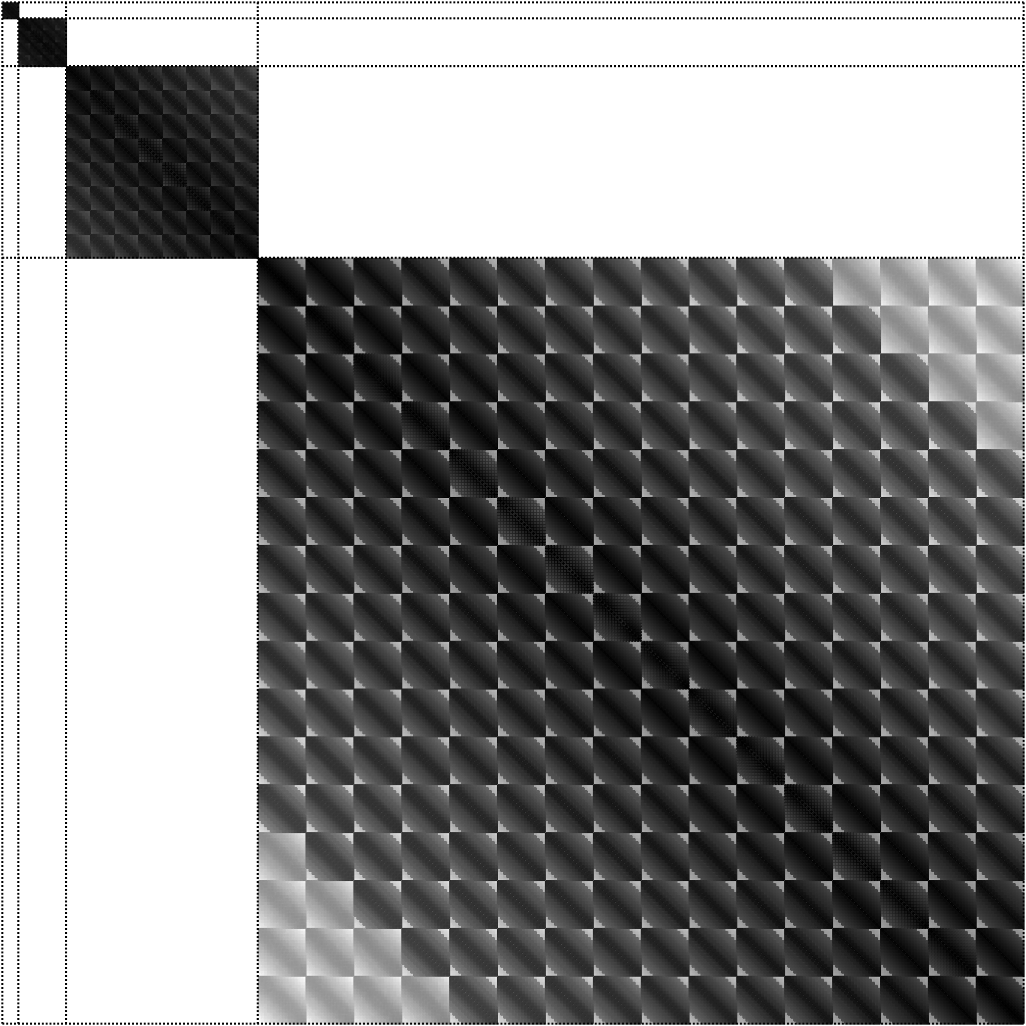
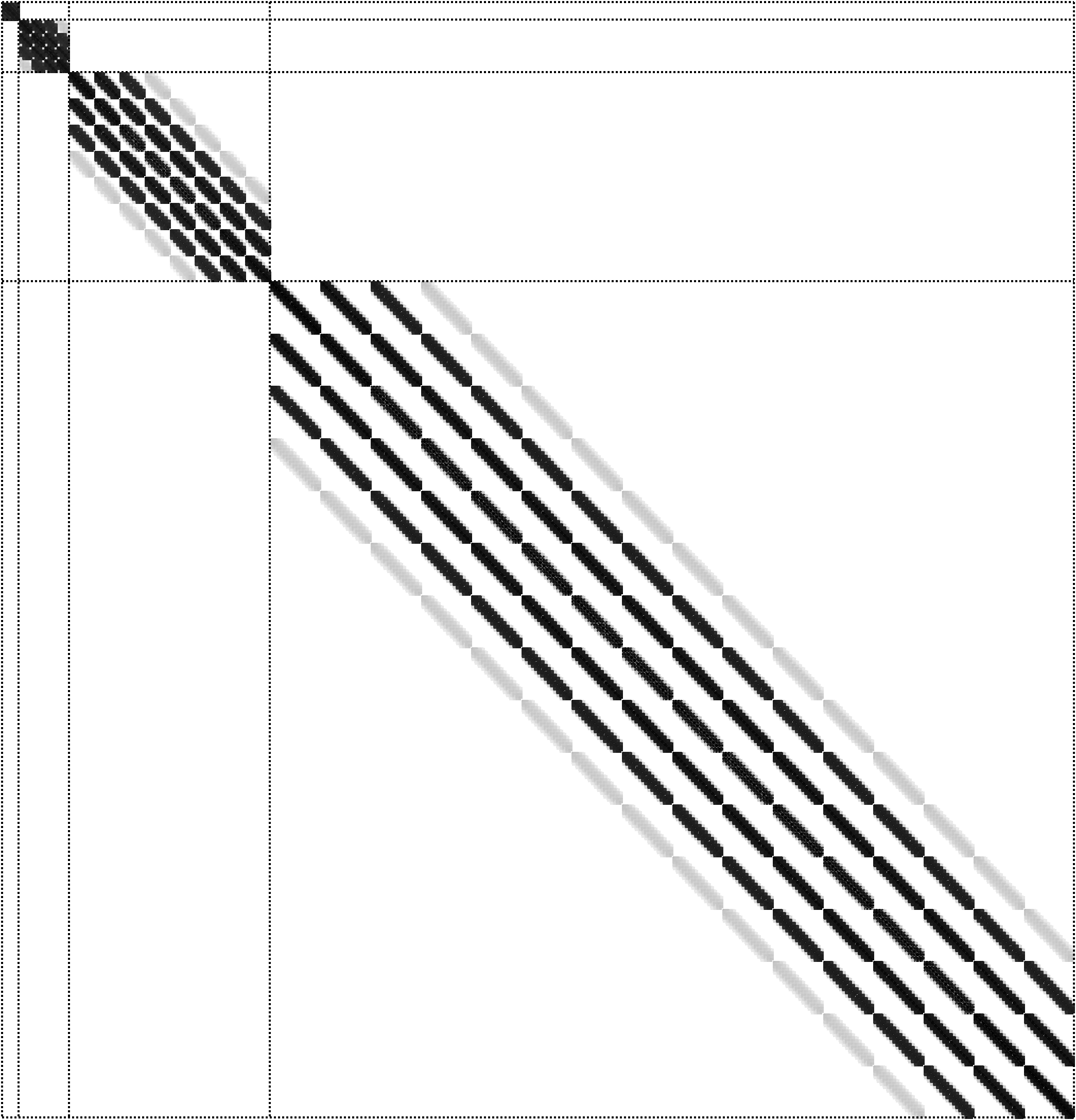
In this section, we introduce localized variants of the hierarchical multi-resolution trial and test spaces from Section 4. The localization procedure results in a practical method with sparse block-diagonal system matrix; see Figure 6.1 for a comparison of the sparsity patterns for the ideal and localized methods.
Refer to caption
Refer to caption
Figure 6.1. Schematic demonstration of the sparsification of the block-diagonal system matrix. Left: Block-matrix corresponding to ideal method (4.5); right: Block-matrix corresponding to proposed practical multi-resolution method (6.3). We use a logarithmic gray-scale as color-coding, where dark gray indicates a large modulo of the corresponding entry; zero entries are colored white.

6.1. Localized trial and test spaces

Here, we introduce the novel localization strategy that improves stability even for the elliptic case. Instead of just replacing the correctors in (4.2) by their localized counterparts, we additionally utilize the operator 𝒫subscript𝒫\mathcal{P}_{\ell} in the definition of the localized trial and test spaces. For =1,,L1𝐿\ell=1,...,L, let

(6.1) Φ~m:=span{(1𝒞m){𝒫Π~ϕ,j,j=1,,N}},Ψ~m:=span{(1𝒞m,){𝒫Π~ϕ,j,j=1,,N}}.\displaystyle\begin{split}\widetilde{\Phi}_{\ell}^{m}&:=\mathrm{span}\big{\{}(1-\mathcal{C}_{\ell}^{m})\{\mathcal{P}_{\ell}\widetilde{\Pi}_{\ell}\phi_{\ell,j},j=1,...,N_{\ell}\}\big{\}},\\ \widetilde{\Psi}_{\ell}^{m}&:=\mathrm{span}\big{\{}(1-\mathcal{C}_{\ell}^{m,*})\{\mathcal{P}_{\ell}\widetilde{\Pi}_{\ell}\phi_{\ell,j},j=1,...,N_{\ell}\}\big{\}}.\end{split}

The canonical bases of Φ~msuperscriptsubscript~Φ𝑚\widetilde{\Phi}_{\ell}^{m} and Ψ~msuperscriptsubscript~Ψ𝑚\widetilde{\Psi}_{\ell}^{m} are given by

(6.2) {b,jm:=(1𝒞m)𝒫Π~ϕ,j,j=1,,N},{b,jm,:=(1𝒞m,)𝒫Π~ϕ,j,j=1,,N}.formulae-sequenceassignsuperscriptsubscript𝑏𝑗𝑚1superscriptsubscript𝒞𝑚subscript𝒫subscript~Πsubscriptitalic-ϕ𝑗𝑗1subscript𝑁formulae-sequenceassignsuperscriptsubscript𝑏𝑗𝑚1superscriptsubscript𝒞𝑚subscript𝒫subscript~Πsubscriptitalic-ϕ𝑗𝑗1subscript𝑁\displaystyle\begin{split}\big{\{}b_{\ell,j}^{m}&:=(1-\mathcal{C}_{\ell}^{m})\mathcal{P}_{\ell}\widetilde{\Pi}_{\ell}\phi_{\ell,j},j=1,...,N_{\ell}\big{\}},\\ \big{\{}b_{\ell,j}^{m,*}&:=(1-\mathcal{C}_{\ell}^{m,*})\mathcal{P}_{\ell}\widetilde{\Pi}_{\ell}\phi_{\ell,j},j=1,...,N_{\ell}\big{\}}.\end{split}
Refer to caption Refer to caption Refer to caption Refer to caption
Figure 6.2. Let the mesh hierarchy be as for Figure 3.1. The pictures show the real part of one (randomly chosen) basis function b,j1superscriptsubscript𝑏𝑗1b_{\ell,j}^{1} per level. The corresponding Haar basis functions ϕ,jsubscriptitalic-ϕ𝑗\phi_{\ell,j} are indicated in green.
Remark 6.1 (Effect of operator 𝒫subscript𝒫\mathcal{P}_{\ell}).

Since 𝒫subscript𝒫\mathcal{P}_{\ell} preserves element-averages, we have (1𝒞l)Π~ϕ=(1𝒞)𝒫Π~ϕ1subscript𝒞𝑙~Πsubscriptitalic-ϕ1subscript𝒞subscript𝒫subscript~Πsubscriptitalic-ϕ(1-\mathcal{C}_{l})\widetilde{\Pi}\phi_{\ell}=(1-\mathcal{C}_{\ell})\mathcal{P}_{\ell}\widetilde{\Pi}_{\ell}\phi_{\ell} for all ϕspan{}subscriptitalic-ϕspansubscript\phi_{\ell}\in\mathrm{span}\{\mathcal{H}_{\ell}\} (analogously for 𝒞superscriptsubscript𝒞\mathcal{C}_{\ell}^{*}). Thus, (6.1) is consistent with (4.2) in the ideal (non-localized) case. The trial and test spaces (6.1) define a method that is uniformly stable in Hsubscript𝐻H_{\ell}. In contrast, omitting 𝒫subscript𝒫\mathcal{P}_{\ell} in (6.1) would result in a method, where the oversampling parameter m𝑚m had to be increased if H1subscript𝐻1H_{1} was decreased; see [34, 33, 27].

Remark 6.2 (Optimality of exponential decay of basis functions).

In the recent work [23], a multi-scale basis is constructed with super-exponential localization properties. While some theoretical aspects are still unclear, numerical experiments show the supremacy of the novel localization approach compared to existing approaches.

Remark 6.3 (Exponential smallness of off-diagonal blocks).

After localization, the operator is not exactly block-diagonal anymore. However, it can be shown that the off-diagonal blocks are exponentially small; see proof of Theorem 6.5. Thus, for sufficiently large m𝑚m, this error does not impact stability and convergence results.

Let us propose the practical variant of the multi-level method (4.5), (4.6): First, on every level, solve Petrov-Galerkin problems, which seek φ~mΦ~msuperscriptsubscript~𝜑𝑚superscriptsubscript~Φ𝑚\tilde{\varphi}_{\ell}^{m}\in\widetilde{\Phi}_{\ell}^{m}, such that for all ψ~mΨ~msuperscriptsubscript~𝜓𝑚superscriptsubscript~Ψ𝑚\tilde{\psi}_{\ell}^{m}\in\widetilde{\Psi}_{\ell}^{m}

(6.3) a(φ~m,ψ~m)=(f,ψ~m)L2(D).𝑎superscriptsubscript~𝜑𝑚superscriptsubscript~𝜓𝑚subscript𝑓superscriptsubscript~𝜓𝑚superscript𝐿2𝐷a(\tilde{\varphi}_{\ell}^{m},\tilde{\psi}_{\ell}^{m})=(f,\tilde{\psi}_{\ell}^{m})_{L^{2}(D)}.

Second, define the solution as the sum of the level contributions

(6.4) u~m:=φ~1m++φ~Lm.assignsuperscript~𝑢𝑚superscriptsubscript~𝜑1𝑚superscriptsubscript~𝜑𝐿𝑚\tilde{u}^{m}:=\tilde{\varphi}_{1}^{m}+...+\tilde{\varphi}_{L}^{m}.

6.2. Stability and accuracy of the practical multi-level method

Provided that the localized method is sufficiently close to the ideal method, the stability and convergence results of the ideal method (Lemma 4.6 and 4.7) carry over to the localized method. The closeness is ensured by a coupling of the oversampling parameter m𝑚m to the stability constant cstab(κ)subscript𝑐stab𝜅c_{\mathrm{stab}}(\kappa). We assume a polynomial dependence of the stability constant on the wave number κ𝜅\kappa; for a discussion of this assumption, see Section 2.

Assumption 6.4 (Polynomial-in-κ𝜅\kappa stability).

We assume that cstabsubscript𝑐stabc_{\mathrm{stab}} depends polynomially on κ𝜅\kappa, i.e.,

cstab(κ)κn.less-than-or-similar-tosubscript𝑐stab𝜅superscript𝜅𝑛c_{\mathrm{stab}}(\kappa)\lesssim\kappa^{n}.
Theorem 6.5 (Stability of localized sub-scale problems).

Let Assumption 4.1 and 6.4 be satisfied, as well as the oversampling condition

(6.5) m|log(β)|1|log(κn+1cm)|greater-than-or-equivalent-to𝑚superscript𝛽1superscript𝜅𝑛1subscript𝑐𝑚m\gtrsim|\log(\beta)|^{-1}|\log(\kappa^{n+1}c_{m})|

with β𝛽\beta and cmsubscript𝑐𝑚c_{m} from Lemma 5.4. Then, for 1,,L1𝐿\ell 1,...,L, the trial space Φ~msuperscriptsubscript~Φ𝑚\widetilde{\Phi}_{\ell}^{m} and the test space Ψ~msuperscriptsubscript~Ψ𝑚\widetilde{\Psi}_{\ell}^{m} satisfy the inf-sup condition

0<α(4)infφ~mΦ~msupψ~mΨ~ma(φ~m,ψ~m)φ~m𝒱(D)ψ~m𝒱(D),0subscriptsuperscript𝛼4subscriptinfimumsuperscriptsubscript~𝜑𝑚superscriptsubscript~Φ𝑚subscriptsupremumsuperscriptsubscript~𝜓𝑚superscriptsubscript~Ψ𝑚𝑎superscriptsubscript~𝜑𝑚superscriptsubscript~𝜓𝑚subscriptnormsuperscriptsubscript~𝜑𝑚𝒱𝐷subscriptnormsuperscriptsubscript~𝜓𝑚𝒱𝐷0<\alpha^{(4)}_{\ell}\leq\inf_{\tilde{\varphi}_{\ell}^{m}\in\widetilde{\Phi}_{\ell}^{m}}\sup_{\tilde{\psi}_{\ell}^{m}\in\widetilde{\Psi}_{\ell}^{m}}\frac{\mathfrak{R}a(\tilde{\varphi}_{\ell}^{m},\tilde{\psi}_{\ell}^{m})}{{\|\tilde{\varphi}_{\ell}^{m}\|}_{\mathcal{V}(D)}{\|\tilde{\psi}_{\ell}^{m}\|}_{\mathcal{V}(D)}},

where α(4)α(3)similar-to-or-equalssubscriptsuperscript𝛼4subscriptsuperscript𝛼3\alpha^{(4)}_{\ell}\simeq\alpha^{(3)}_{\ell}, with constants α(3)subscriptsuperscript𝛼3\alpha^{(3)}_{\ell} from Remark 4.12 (=1)1(\ell=1) and Lemma 4.11 (2)2(\ell\geq 2).

Proof.

Let {1,,L}1𝐿\ell\in\{1,...,L\} be fixed and let φ~mΦ~msuperscriptsubscript~𝜑𝑚superscriptsubscript~Φ𝑚\tilde{\varphi}_{\ell}^{m}\in\widetilde{\Phi}_{\ell}^{m} be arbitrary. Define φ~:=(1𝒞)𝒫φ~massignsubscript~𝜑1subscript𝒞subscript𝒫superscriptsubscript~𝜑𝑚\tilde{\varphi}_{\ell}:=(1-\mathcal{C}_{\ell})\mathcal{P}_{\ell}\tilde{\varphi}_{\ell}^{m} and ψ~m:=(1𝒞m,)𝒫ψ~assignsuperscriptsubscript~𝜓𝑚1superscriptsubscript𝒞𝑚subscript𝒫subscript~𝜓\tilde{\psi}_{\ell}^{m}:=(1-\mathcal{C}_{\ell}^{m,*})\mathcal{P}_{\ell}\tilde{\psi}_{\ell}, where ψ~Ψ~subscript~𝜓subscript~Ψ\tilde{\psi}_{\ell}\in\widetilde{\Psi}_{\ell} is chosen such that (Lemma 4.11)

a(φ~,ψ~)α(3)φ~𝒱(D)ψ~𝒱(D).𝑎subscript~𝜑subscript~𝜓subscriptsuperscript𝛼3subscriptdelimited-∥∥subscript~𝜑𝒱𝐷subscriptnormsubscript~𝜓𝒱𝐷\mathfrak{R}a(\tilde{\varphi}_{\ell},\tilde{\psi}_{\ell})\geq\alpha^{(3)}_{\ell}{\left\lVert\tilde{\varphi}_{\ell}\right\rVert}_{\mathcal{V}(D)}{\|\tilde{\psi}_{\ell}\|}_{\mathcal{V}(D)}.

We obtain

a(φ~m,ψ~m)=a(φ~m,ψ~)+a(φ~m,ψ~mψ~)=a(φ~,ψ~)+a(φ~m,ψ~mψ~).𝑎superscriptsubscript~𝜑𝑚superscriptsubscript~𝜓𝑚𝑎superscriptsubscript~𝜑𝑚subscript~𝜓𝑎superscriptsubscript~𝜑𝑚superscriptsubscript~𝜓𝑚subscript~𝜓𝑎subscript~𝜑subscript~𝜓𝑎superscriptsubscript~𝜑𝑚superscriptsubscript~𝜓𝑚subscript~𝜓\displaystyle\mathfrak{R}a(\tilde{\varphi}_{\ell}^{m},\tilde{\psi}_{\ell}^{m})=\mathfrak{R}a(\tilde{\varphi}_{\ell}^{m},\tilde{\psi}_{\ell})+\mathfrak{R}a(\tilde{\varphi}_{\ell}^{m},\tilde{\psi}_{\ell}^{m}-\tilde{\psi}_{\ell})=\mathfrak{R}a(\tilde{\varphi}_{\ell},\tilde{\psi}_{\ell})+\mathfrak{R}a(\tilde{\varphi}_{\ell}^{m},\tilde{\psi}_{\ell}^{m}-\tilde{\psi}_{\ell}).

The second term can be bounded by

|a(φ~m,ψ~mψ~)|𝑎superscriptsubscript~𝜑𝑚superscriptsubscript~𝜓𝑚subscript~𝜓\displaystyle\big{|}\mathfrak{R}a(\tilde{\varphi}_{\ell}^{m},\tilde{\psi}_{\ell}^{m}-\tilde{\psi}_{\ell})\big{|} φ~m𝒱(D)ψ~mψ~𝒱(D)=φ~m𝒱(D)(𝒞m,𝒞)𝒫ψ~𝒱(D)less-than-or-similar-toabsentsubscriptnormsuperscriptsubscript~𝜑𝑚𝒱𝐷subscriptnormsuperscriptsubscript~𝜓𝑚subscript~𝜓𝒱𝐷subscriptnormsuperscriptsubscript~𝜑𝑚𝒱𝐷subscriptnormsuperscriptsubscript𝒞𝑚superscriptsubscript𝒞subscript𝒫subscript~𝜓𝒱𝐷\displaystyle\lesssim{\|\tilde{\varphi}_{\ell}^{m}\|}_{\mathcal{V}(D)}{\|\tilde{\psi}_{\ell}^{m}-\tilde{\psi}_{\ell}\|}_{\mathcal{V}(D)}={\|\tilde{\varphi}_{\ell}^{m}\|}_{\mathcal{V}(D)}{\|(\mathcal{C}_{\ell}^{m,*}-\mathcal{C}_{\ell}^{*})\mathcal{P}_{\ell}\tilde{\psi}_{\ell}\|}_{\mathcal{V}(D)}
cmβmφ~m𝒱(D)ψ~𝒱(D).less-than-or-similar-toabsentsubscript𝑐𝑚superscript𝛽𝑚subscriptnormsuperscriptsubscript~𝜑𝑚𝒱𝐷subscriptnormsubscript~𝜓𝒱𝐷\displaystyle\lesssim c_{m}\beta^{m}{\|\tilde{\varphi}_{\ell}^{m}\|}_{\mathcal{V}(D)}{\|\tilde{\psi}_{\ell}\|}_{\mathcal{V}(D)}.

It remains to estimate the 𝒱𝒱\mathcal{V}-norm of φ~subscript~𝜑\tilde{\varphi}_{\ell} and ψ~subscript~𝜓\tilde{\psi}_{\ell} against the 𝒱𝒱\mathcal{V}-norm of its localized counterparts and vice-versa. With (3.4) and Remark 4.3, we obtain

φ~𝒱(D)=(1𝒞)𝒫φ~m𝒱(D)𝒫φ~m𝒱(D)φ~m𝒱(D),subscriptnormsubscript~𝜑𝒱𝐷subscriptnorm1subscript𝒞subscript𝒫superscriptsubscript~𝜑𝑚𝒱𝐷less-than-or-similar-tosubscriptnormsubscript𝒫superscriptsubscript~𝜑𝑚𝒱𝐷less-than-or-similar-tosubscriptnormsuperscriptsubscript~𝜑𝑚𝒱𝐷\displaystyle{\|\tilde{\varphi}_{\ell}\|}_{\mathcal{V}(D)}={\|(1-\mathcal{C}_{\ell})\mathcal{P}_{\ell}\tilde{\varphi}_{\ell}^{m}\|}_{\mathcal{V}(D)}\lesssim{\|\mathcal{P}_{\ell}\tilde{\varphi}_{\ell}^{m}\|}_{\mathcal{V}(D)}\lesssim{\|\tilde{\varphi}_{\ell}^{m}\|}_{\mathcal{V}(D)},

Furthermore, with Lemma 5.4, we get

φ~m𝒱(D)subscriptnormsuperscriptsubscript~𝜑𝑚𝒱𝐷\displaystyle{\|\tilde{\varphi}_{\ell}^{m}\|}_{\mathcal{V}(D)} =(1𝒞m)𝒫φ~m𝒱(D)(1𝒞)𝒫φ~m𝒱(D)+(𝒞m𝒞)𝒫φ~m𝒱(D)absentsubscriptnorm1superscriptsubscript𝒞𝑚subscript𝒫superscriptsubscript~𝜑𝑚𝒱𝐷subscriptnorm1subscript𝒞subscript𝒫superscriptsubscript~𝜑𝑚𝒱𝐷subscriptnormsuperscriptsubscript𝒞𝑚subscript𝒞subscript𝒫superscriptsubscript~𝜑𝑚𝒱𝐷\displaystyle={\|(1-\mathcal{C}_{\ell}^{m})\mathcal{P}_{\ell}\tilde{\varphi}_{\ell}^{m}\|}_{\mathcal{V}(D)}\leq{\|(1-\mathcal{C}_{\ell})\mathcal{P}_{\ell}\tilde{\varphi}_{\ell}^{m}\|}_{\mathcal{V}(D)}+{\|(\mathcal{C}_{\ell}^{m}-\mathcal{C}_{\ell})\mathcal{P}_{\ell}\tilde{\varphi}_{\ell}^{m}\|}_{\mathcal{V}(D)}
φ~𝒱(D)+cmβm𝒫φ~m𝒱(D)(1+cmβm)φ~𝒱(D)φ~𝒱(D),less-than-or-similar-toabsentsubscriptnormsubscript~𝜑𝒱𝐷subscript𝑐𝑚superscript𝛽𝑚subscriptnormsubscript𝒫superscriptsubscript~𝜑𝑚𝒱𝐷less-than-or-similar-to1subscript𝑐𝑚superscript𝛽𝑚subscriptnormsubscript~𝜑𝒱𝐷less-than-or-similar-tosubscriptnormsubscript~𝜑𝒱𝐷\displaystyle\lesssim{\|\tilde{\varphi}_{\ell}\|}_{\mathcal{V}(D)}+c_{m}\beta^{m}{\|\mathcal{P}_{\ell}\tilde{\varphi}_{\ell}^{m}\|}_{\mathcal{V}(D)}\lesssim(1+c_{m}\beta^{m}){\|\tilde{\varphi}_{\ell}\|}_{\mathcal{V}(D)}\lesssim{\|\tilde{\varphi}_{\ell}\|}_{\mathcal{V}(D)},

where we used that cmβmsubscript𝑐𝑚superscript𝛽𝑚c_{m}\beta^{m} can be bounded independently of m𝑚m. The corresponding estimates for ψ~subscript~𝜓\tilde{\psi}_{\ell} and ψ~msuperscriptsubscript~𝜓𝑚\tilde{\psi}_{\ell}^{m} can be obtained using similar arguments.

We conclude

a(φ~m,ψ~m)𝑎superscriptsubscript~𝜑𝑚superscriptsubscript~𝜓𝑚\displaystyle\mathfrak{R}a(\tilde{\varphi}_{\ell}^{m},\tilde{\psi}_{\ell}^{m}) =a(φ~,ψ~)+a(φ~m,ψ~mψ~)absent𝑎subscript~𝜑subscript~𝜓𝑎superscriptsubscript~𝜑𝑚superscriptsubscript~𝜓𝑚subscript~𝜓\displaystyle=\mathfrak{R}a(\tilde{\varphi}_{\ell},\tilde{\psi}_{\ell})+\mathfrak{R}a(\tilde{\varphi}_{\ell}^{m},\tilde{\psi}_{\ell}^{m}-\tilde{\psi}_{\ell})
α(3)φ~𝒱(D)ψ~𝒱(D)cmβmφ~m𝒱(D)ψ~𝒱(D)greater-than-or-equivalent-toabsentsubscriptsuperscript𝛼3subscriptnormsubscript~𝜑𝒱𝐷subscriptnormsubscript~𝜓𝒱𝐷subscript𝑐𝑚superscript𝛽𝑚subscriptnormsuperscriptsubscript~𝜑𝑚𝒱𝐷subscriptnormsubscript~𝜓𝒱𝐷\displaystyle\gtrsim\alpha^{(3)}_{\ell}{\|\tilde{\varphi}_{\ell}\|}_{\mathcal{V}(D)}{\|\tilde{\psi}_{\ell}\|}_{\mathcal{V}(D)}-c_{m}\beta^{m}{\|\tilde{\varphi}_{\ell}^{m}\|}_{\mathcal{V}(D)}{\|\tilde{\psi}_{\ell}\|}_{\mathcal{V}(D)}
(α(3)cmβm)φ~m𝒱(D)ψ~m𝒱(D)greater-than-or-equivalent-toabsentsubscriptsuperscript𝛼3subscript𝑐𝑚superscript𝛽𝑚subscriptnormsuperscriptsubscript~𝜑𝑚𝒱𝐷subscriptnormsuperscriptsubscript~𝜓𝑚𝒱𝐷\displaystyle\gtrsim(\alpha^{(3)}_{\ell}-c_{m}\beta^{m}){\|\tilde{\varphi}_{\ell}^{m}\|}_{\mathcal{V}(D)}{\|\tilde{\psi}_{\ell}^{m}\|}_{\mathcal{V}(D)}
α(3)φ~m𝒱(D)ψ~m𝒱(D).greater-than-or-equivalent-toabsentsubscriptsuperscript𝛼3subscriptnormsuperscriptsubscript~𝜑𝑚𝒱𝐷subscriptnormsuperscriptsubscript~𝜓𝑚𝒱𝐷\displaystyle\gtrsim\alpha^{(3)}_{\ell}{\|\tilde{\varphi}_{\ell}^{m}\|}_{\mathcal{V}(D)}{\|\tilde{\psi}_{\ell}^{m}\|}_{\mathcal{V}(D)}.

In the last inequality, we employed the oversampling condition (6.5). ∎

Remark 6.6 (Level oversampling parameter).

In the proof of Theorem 6.5, it is possible to relax oversampling condition (6.5), choosing level-dependent oversampling parameters

m|log(β)|1{|log(κn+1cm)| for =1,|log(cm)| for 2.greater-than-or-equivalent-tosubscript𝑚superscript𝛽1casessuperscript𝜅𝑛1subscript𝑐𝑚 for 1subscript𝑐𝑚 for 2\displaystyle m_{\ell}\gtrsim|\log(\beta)|^{-1}\cdot\begin{cases}|\log(\kappa^{n+1}c_{m})|\quad&\text{ for }\ell=1,\\ |\log(c_{m})|\quad&\text{ for }\ell\geq 2.\end{cases}
Theorem 6.7 (A-priori error estimate).

Let u𝒱𝑢𝒱u\in\mathcal{V} be the solution of (2.3) for the right-hand side f𝑓f. If Assumption 4.1 and 6.4 are satisfied as well as the oversampling condition (6.5), then is a constant cκ,m,Lsubscript𝑐𝜅𝑚𝐿c_{\kappa,m,L} depending polynomially on κ𝜅\kappa, m𝑚m and linearly on L𝐿L, but independent of HLsubscript𝐻𝐿H_{L} such that the solution of the proposed practical multi-level method (6.3), (6.4) satisfies for any fHs(D)𝑓superscript𝐻𝑠𝐷f\in H^{s}(D), s[0,1]𝑠01s\in[0,1]

(6.6) uu~m𝒱(D)HL1+sfHs(D)+cκ,m,LβmfL2(D).less-than-or-similar-tosubscriptdelimited-∥∥𝑢superscript~𝑢𝑚𝒱𝐷superscriptsubscript𝐻𝐿1𝑠subscriptnorm𝑓superscript𝐻𝑠𝐷subscript𝑐𝜅𝑚𝐿superscript𝛽𝑚subscriptdelimited-∥∥𝑓superscript𝐿2𝐷{\left\lVert u-\tilde{u}^{m}\right\rVert}_{\mathcal{V}(D)}\lesssim H_{L}^{1+s}\|f\|_{H^{s}(D)}+c_{\kappa,m,L}\beta^{m}{\left\lVert f\right\rVert}_{L^{2}(D)}.
Proof.

We first estimate using the triangle inequality

uu~m𝒱(D)uu~𝒱(D)+u~mu~𝒱(D)uu~𝒱(D)+=1Lφ~mφ~𝒱(D)subscriptdelimited-∥∥𝑢superscript~𝑢𝑚𝒱𝐷subscriptdelimited-∥∥𝑢~𝑢𝒱𝐷subscriptdelimited-∥∥superscript~𝑢𝑚~𝑢𝒱𝐷subscriptdelimited-∥∥𝑢~𝑢𝒱𝐷superscriptsubscript1𝐿subscriptdelimited-∥∥superscriptsubscript~𝜑𝑚subscript~𝜑𝒱𝐷{\left\lVert u-\tilde{u}^{m}\right\rVert}_{\mathcal{V}(D)}\leq{\left\lVert u-\tilde{u}\right\rVert}_{\mathcal{V}(D)}+{\left\lVert\tilde{u}^{m}-\tilde{u}\right\rVert}_{\mathcal{V}(D)}\leq{\left\lVert u-\tilde{u}\right\rVert}_{\mathcal{V}(D)}+\sum_{\ell=1}^{L}{\left\lVert\tilde{\varphi}_{\ell}^{m}-\tilde{\varphi}_{\ell}\right\rVert}_{\mathcal{V}(D)}

with φ~mΦ~msuperscriptsubscript~𝜑𝑚superscriptsubscript~Φ𝑚\tilde{\varphi}_{\ell}^{m}\in\widetilde{\Phi}_{\ell}^{m} solving (6.3). The first term can be estimated with Lemma 4.7. The functions φ~msuperscriptsubscript~𝜑𝑚\tilde{\varphi}_{\ell}^{m} are non-conforming, non-consistent Petrov-Galerkin approximations of φ~Φ~subscript~𝜑subscript~Φ\tilde{\varphi}_{\ell}\in\widetilde{\Phi}_{\ell} solving (4.5). Using Strang’s Lemma (c.f. [24]) yields

α(4)φ~mφ~𝒱(D)subscriptsuperscript𝛼4subscriptdelimited-∥∥superscriptsubscript~𝜑𝑚subscript~𝜑𝒱𝐷\displaystyle\alpha^{(4)}_{\ell}{\left\lVert\tilde{\varphi}_{\ell}^{m}-\tilde{\varphi}_{\ell}\right\rVert}_{\mathcal{V}(D)} infφ~mΦ~mφ~mφ~𝒱(D)+supψ~mΨ~m|a(φ~,ψ~m)(f,ψ~m)L2(D)|ψ~m𝒱(D)less-than-or-similar-toabsentsubscriptinfimumsuperscriptsubscript~𝜑𝑚superscriptsubscript~Φ𝑚subscriptdelimited-∥∥superscriptsubscript~𝜑𝑚subscript~𝜑𝒱𝐷subscriptsupremumsuperscriptsubscript~𝜓𝑚superscriptsubscript~Ψ𝑚𝑎subscript~𝜑superscriptsubscript~𝜓𝑚subscript𝑓superscriptsubscript~𝜓𝑚superscript𝐿2𝐷subscriptnormsuperscriptsubscript~𝜓𝑚𝒱𝐷\displaystyle\lesssim\inf_{\tilde{\varphi}_{\ell}^{m}\in\widetilde{\Phi}_{\ell}^{m}}{\left\lVert\tilde{\varphi}_{\ell}^{m}-\tilde{\varphi}_{\ell}\right\rVert}_{\mathcal{V}(D)}+\sup_{\tilde{\psi}_{\ell}^{m}\in\widetilde{\Psi}_{\ell}^{m}}\frac{\big{|}a(\tilde{\varphi}_{\ell},\tilde{\psi}_{\ell}^{m})-{(f\,,\,\tilde{\psi}_{\ell}^{m})}_{L^{2}(D)}\big{|}}{{\|\tilde{\psi}_{\ell}^{m}\|}_{\mathcal{V}(D)}}

For the first term, we choose φ~m:=(1𝒞m)𝒫φ~assignsuperscriptsubscript~𝜑𝑚1superscriptsubscript𝒞𝑚subscript𝒫subscript~𝜑\tilde{\varphi}_{\ell}^{m}:=(1-\mathcal{C}_{\ell}^{m})\mathcal{P}_{\ell}\tilde{\varphi}_{\ell}. Using Lemma 4.11, we get

infφ~mΦ~mφ~mφ~𝒱(D)(𝒞m𝒞)𝒫φ~𝒱(D)cmβmφ~𝒱(D)cmβmα(2),1fL2(D).subscriptinfimumsuperscriptsubscript~𝜑𝑚superscriptsubscript~Φ𝑚subscriptdelimited-∥∥superscriptsubscript~𝜑𝑚subscript~𝜑𝒱𝐷subscriptdelimited-∥∥superscriptsubscript𝒞𝑚subscript𝒞subscript𝒫subscript~𝜑𝒱𝐷less-than-or-similar-tosubscript𝑐𝑚superscript𝛽𝑚subscriptdelimited-∥∥subscript~𝜑𝒱𝐷less-than-or-similar-tosubscript𝑐𝑚superscript𝛽𝑚subscriptsuperscript𝛼21subscriptdelimited-∥∥𝑓superscript𝐿2𝐷\inf_{\tilde{\varphi}_{\ell}^{m}\in\widetilde{\Phi}_{\ell}^{m}}{\left\lVert\tilde{\varphi}_{\ell}^{m}-\tilde{\varphi}_{\ell}\right\rVert}_{\mathcal{V}(D)}\leq{\left\lVert(\mathcal{C}_{\ell}^{m}-\mathcal{C}_{\ell})\mathcal{P}_{\ell}\tilde{\varphi}_{\ell}\right\rVert}_{\mathcal{V}(D)}\lesssim c_{m}\beta^{m}{\left\lVert\tilde{\varphi}_{\ell}\right\rVert}_{\mathcal{V}(D)}\lesssim c_{m}\beta^{m}{\alpha^{(2),-1}_{\ell}}{\left\lVert f\right\rVert}_{L^{2}(D)}.

Let ψ~Ψ~subscript~𝜓subscript~Ψ\tilde{\psi}_{\ell}\in\widetilde{\Psi}_{\ell} be arbitrary. Then, for the second term, we obtain after some algebraic manipulations

a(φ~,ψ~m)𝑎subscript~𝜑superscriptsubscript~𝜓𝑚\displaystyle a(\tilde{\varphi}_{\ell},\tilde{\psi}_{\ell}^{m}) (f,ψ~m)L2(D)=a(φ~,ψ~m)a(φ~m,ψ~m)=a(φ~,ψ~)a(φ~m,ψ~m)+subscript𝑓superscriptsubscript~𝜓𝑚superscript𝐿2𝐷𝑎subscript~𝜑superscriptsubscript~𝜓𝑚𝑎superscriptsubscript~𝜑𝑚superscriptsubscript~𝜓𝑚𝑎subscript~𝜑subscript~𝜓limit-from𝑎superscriptsubscript~𝜑𝑚superscriptsubscript~𝜓𝑚\displaystyle-{(f\,,\,\tilde{\psi}_{\ell}^{m})}_{L^{2}(D)}=a(\tilde{\varphi}_{\ell},\tilde{\psi}_{\ell}^{m})-a(\tilde{\varphi}_{\ell}^{m},\tilde{\psi}_{\ell}^{m})=a(\tilde{\varphi}_{\ell},\tilde{\psi}_{\ell})-a(\tilde{\varphi}_{\ell}^{m},\tilde{\psi}_{\ell}^{m})+
+a(φ~,ψ~mψ~)=(f,ψ~ψ~m)L2(D)+a(φ~,ψ~mψ~).𝑎subscript~𝜑superscriptsubscript~𝜓𝑚subscript~𝜓subscript𝑓subscript~𝜓superscriptsubscript~𝜓𝑚superscript𝐿2𝐷𝑎subscript~𝜑superscriptsubscript~𝜓𝑚subscript~𝜓\displaystyle+a(\tilde{\varphi}_{\ell},\tilde{\psi}_{\ell}^{m}-\tilde{\psi}_{\ell})={(f\,,\,\tilde{\psi}_{\ell}-\tilde{\psi}_{\ell}^{m})}_{L^{2}(D)}+a(\tilde{\varphi}_{\ell},\tilde{\psi}_{\ell}^{m}-\tilde{\psi}_{\ell}).

The choice ψ~:=(1𝒞)𝒫ψ~massignsubscript~𝜓1superscriptsubscript𝒞subscript𝒫superscriptsubscript~𝜓𝑚\tilde{\psi}_{\ell}:=(1-\mathcal{C}_{\ell}^{*})\mathcal{P}_{\ell}\tilde{\psi}_{\ell}^{m} yields

|a(φ~,ψ~m)(f,ψ~m)L2(D)|𝑎subscript~𝜑superscriptsubscript~𝜓𝑚subscript𝑓superscriptsubscript~𝜓𝑚superscript𝐿2𝐷\displaystyle\big{|}a(\tilde{\varphi}_{\ell},\tilde{\psi}_{\ell}^{m})-{(f\,,\,\tilde{\psi}_{\ell}^{m})}_{L^{2}(D)}\big{|} κ01fL2(D)ψ~mψ~𝒱(D)+φ~𝒱(D)ψ~mψ~𝒱(D)less-than-or-similar-toabsentsuperscriptsubscript𝜅01subscriptdelimited-∥∥𝑓superscript𝐿2𝐷subscriptnormsuperscriptsubscript~𝜓𝑚subscript~𝜓𝒱𝐷subscriptdelimited-∥∥subscript~𝜑𝒱𝐷subscriptnormsuperscriptsubscript~𝜓𝑚subscript~𝜓𝒱𝐷\displaystyle\lesssim\kappa_{0}^{-1}{\left\lVert f\right\rVert}_{L^{2}(D)}{\|\tilde{\psi}_{\ell}^{m}-\tilde{\psi}_{\ell}\|}_{\mathcal{V}(D)}+{\left\lVert\tilde{\varphi}_{\ell}\right\rVert}_{\mathcal{V}(D)}{\|\tilde{\psi}_{\ell}^{m}-\tilde{\psi}_{\ell}\|}_{\mathcal{V}(D)}
(κ01+α(3),1)fL2(D)(𝒞m,𝒞m)𝒫ψ~m𝒱(D)less-than-or-similar-toabsentsuperscriptsubscript𝜅01subscriptsuperscript𝛼31subscriptdelimited-∥∥𝑓superscript𝐿2𝐷subscriptnormsuperscriptsubscript𝒞𝑚superscriptsubscript𝒞𝑚subscript𝒫superscriptsubscript~𝜓𝑚𝒱𝐷\displaystyle\lesssim\big{(}\kappa_{0}^{-1}+{\alpha^{(3),-1}_{\ell}}\big{)}{\left\lVert f\right\rVert}_{L^{2}(D)}{\|(\mathcal{C}_{\ell}^{m,*}-\mathcal{C}_{\ell}^{m})\mathcal{P}_{\ell}\tilde{\psi}_{\ell}^{m}\|}_{\mathcal{V}(D)}
cmβm(κ01+α(3),1)fL2(D)ψ~m𝒱(D).less-than-or-similar-toabsentsubscript𝑐𝑚superscript𝛽𝑚superscriptsubscript𝜅01subscriptsuperscript𝛼31subscriptdelimited-∥∥𝑓superscript𝐿2𝐷subscriptnormsuperscriptsubscript~𝜓𝑚𝒱𝐷\displaystyle\lesssim c_{m}\beta^{m}\big{(}\kappa_{0}^{-1}+{\alpha^{(3),-1}_{\ell}}\big{)}{\left\lVert f\right\rVert}_{L^{2}(D)}{\|\tilde{\psi}_{\ell}^{m}\|}_{\mathcal{V}(D)}.

After dividing by ψ~m𝒱(D)subscriptnormsuperscriptsubscript~𝜓𝑚𝒱𝐷{\|\tilde{\psi}_{\ell}^{m}\|}_{\mathcal{V}(D)}, the desired estimate follows. Combining both estimates, we obtain

φ~mφ~𝒱(D)c,m,κβmfL2(D) with c,m,κ:=cmα(4),1(κ01+α(3),1).formulae-sequenceless-than-or-similar-tosubscriptdelimited-∥∥superscriptsubscript~𝜑𝑚subscript~𝜑𝒱𝐷subscript𝑐𝑚𝜅superscript𝛽𝑚subscriptdelimited-∥∥𝑓superscript𝐿2𝐷 with assignsubscript𝑐𝑚𝜅subscript𝑐𝑚subscriptsuperscript𝛼41superscriptsubscript𝜅01subscriptsuperscript𝛼31\displaystyle{\left\lVert\tilde{\varphi}_{\ell}^{m}-\tilde{\varphi}_{\ell}\right\rVert}_{\mathcal{V}(D)}\lesssim c_{\ell,m,\kappa}\beta^{m}{\left\lVert f\right\rVert}_{L^{2}(D)}\quad\text{ with }\quad c_{\ell,m,\kappa}:=c_{m}\alpha^{(4),-1}_{\ell}\big{(}\kappa_{0}^{-1}+\alpha^{(3),-1}_{\ell}\big{)}.

Using Lemma 4.11, Remark 4.12, and Theorem 6.5, we can derive the bounds c1,m,κcmκ2n+2less-than-or-similar-tosubscript𝑐1𝑚𝜅subscript𝑐𝑚superscript𝜅2𝑛2c_{1,m,\kappa}\lesssim c_{m}\kappa^{2n+2} for =11\ell=1 and c,m,κcmless-than-or-similar-tosubscript𝑐𝑚𝜅subscript𝑐𝑚c_{\ell,m,\kappa}\lesssim c_{m} for 22\ell\geq 2. Summing over all levels proves the assertion with the constant

cκ,m,L:=cm(κ2n+2+L).assignsubscript𝑐𝜅𝑚𝐿subscript𝑐𝑚superscript𝜅2𝑛2𝐿c_{\kappa,m,L}:=c_{m}(\kappa^{2n+2}+L).

Remark 6.8 (Oversampling).

If the oversampling parameter, in addition to (6.5), also satisfies

m|log(β)|1|log(HLcκ,m,L1)|,greater-than-or-equivalent-to𝑚superscript𝛽1subscript𝐻𝐿superscriptsubscript𝑐𝜅𝑚𝐿1m\gtrsim|\log(\beta)|^{-1}|\log(H_{L}c_{\kappa,m,L}^{-1})|,

then the overall error uu~m𝒱(D)subscriptdelimited-∥∥𝑢superscript~𝑢𝑚𝒱𝐷{\left\lVert u-\tilde{u}^{m}\right\rVert}_{\mathcal{V}(D)} in (6.6) is of order 1+s1𝑠1+s in HLsubscript𝐻𝐿H_{L}.

Remark 6.9 (L2superscript𝐿2L^{2}-error estimate).

In Theorem 6.7 an error estimate with respect to the norm 𝒱(D){\|\cdot\|}_{\mathcal{V}(D)} is stated. Defining e:=uu~assign𝑒𝑢~𝑢e:=u-\tilde{u}, an estimate in the weaker L2superscript𝐿2L^{2}-norm can be proved for the ideal method

eL2(D)=(1ΠL)eL2(D)π1HLeL2(D)π1HLe𝒱(D),subscriptnorm𝑒superscript𝐿2𝐷subscriptnorm1subscriptΠ𝐿𝑒superscript𝐿2𝐷superscript𝜋1subscript𝐻𝐿subscriptnorm𝑒superscript𝐿2𝐷superscript𝜋1subscript𝐻𝐿subscriptnorm𝑒𝒱𝐷{\|e\|}_{L^{2}(D)}={\|(1-\Pi_{L})e\|}_{L^{2}(D)}\leq\pi^{-1}H_{L}{\|\nabla e\|}_{L^{2}(D)}\leq\pi^{-1}H_{L}{\|e\|}_{\mathcal{V}(D)},

where we used that e𝒲L𝑒subscript𝒲𝐿e\in\mathcal{W}_{L}. This directly implies convergence of order 2+s2𝑠2+s for the ideal method (4.4) provided that fHs(D)𝑓superscript𝐻𝑠𝐷f\in H^{s}(D). It is straightforward to extend this result to the localized multi-level method, i.e.,

uu~mL2(D)HL2+sfHs(D)+cκ,m,LβmfL2(D).less-than-or-similar-tosubscriptnorm𝑢superscript~𝑢𝑚superscript𝐿2𝐷superscriptsubscript𝐻𝐿2𝑠subscriptnorm𝑓superscript𝐻𝑠𝐷subscript𝑐𝜅𝑚𝐿superscript𝛽𝑚subscriptnorm𝑓superscript𝐿2𝐷\|u-\tilde{u}^{m}\|_{L^{2}(D)}\lesssim H_{L}^{2+s}\|f\|_{H^{s}(D)}+c_{\kappa,m,L}\beta^{m}\|f\|_{L^{2}(D)}.
Remark 6.10 (Comparison to classical Helmholtz analysis).

The analysis of standard finite element discretizations for Helmholtz problems is based on an observation by Schatz [41]. He observed that, if an indefinite sesquilinear form satisfies Gårding’s inequality, the stability and quasi-optimality of a finite element discretization can be shown under the two assumptions: (i) approximation properties of the finite element test space and (ii) a sufficiently small mesh size.

In the original paper introducing the LOD for Helmholtz problems, Schatz’s argument is employed for the error analysis of the localized method; see [37, Theorem 5.5]. However, due to the sophisticated multi-resolution structure of the discrete problem, Schatz’s argument could not be employed in the present work. Nevertheless, using Strang’s lemma and the special properties of the multi-resolution ansatz spaces, we were able to prove similar error estimates also for the multi-resolution method with a slightly larger constant; see Theorem 6.7.

6.3. Practical aspects

The localized element-corrector problems (5.1) are still infinite-dimensional problems and need to be discretized itself. For the ease of presentation, we restrict ourselves in this paper to the classical case of 𝒬1subscript𝒬1\mathcal{Q}_{1} finite elements. We emphasize that a large variety of discretization schemes can be applied, in particular, also hp𝑝hp adaptive methods.

The patch-local corrector problems (5.2) are discretized and solved on a fine mesh of the respective patch with mesh-size hh satisfying that κ2hsuperscript𝜅2\kappa^{2}h is sufficiently small. Under additional geometric requirements, this guarantees stability and quasi-uniformity of the 𝒬1subscript𝒬1\mathcal{Q}_{1} finite element discretization; see [29]. Note that all element-corrector problems are independent and thus, can be solved in parallel. The number of fine-scale problems to be solved on level \ell is independent of subscript\mathcal{H}_{\ell} and only depends on the oversampling parameter m𝑚m. In Lemma 4.2, it was shown that the corrector problems are coercive. However, this is not a real practical benefit, since the spaces 𝒲subscript𝒲\mathcal{W}_{\ell} are difficult to construct numerically. It is more practicable to derive a saddle point formulation of the problem with constraints enforcing that the solution is in 𝒲subscript𝒲\mathcal{W}_{\ell}. The number of constraints (##\#c) is small and only depends polynomially on m𝑚m.

The solution procedure proposed in [31] computes ##\#c Helmholtz problems on every (reference) patch. Since the patches have a diameter at most of order mH1𝑚subscript𝐻1mH_{1}, the effective wave number of the patch problems is at most of order m𝑚m (Assumption 4.1). For such Helmholtz problems, there exist effective preconditioners; see [14, 19, 39]. With the solution of the Helmholtz patch problems at hand, it is then possible to calculate the Schur complement explicitly. For a more detailed discussion of the numerical solution of the corrector problems, see [10, 31].

7. Fast solvers

In this section, we propose a strategy for solving the level problems (6.3) efficiently. As Remark 6.6 already indicates, for 22\ell\geq 2, problems (6.3) are good-natured in the sense that it can be solved up to a given tolerance within a fixed number of GMRES steps (Theorem 7.1). However, for =11\ell=1, the κ𝜅\kappa-dependence in Remark 6.6 makes this impossible. Since this block is relatively small, we suggest a direct solver for the first block.

Recalling the choice of bases (6.2), we can rewrite (6.3) for =1,,L1𝐿\ell=1,...,L into (decoupled) linear systems of equations

(7.1) 𝐀m𝐱m=𝐟msubscriptsuperscript𝐀𝑚superscriptsubscript𝐱𝑚superscriptsubscript𝐟𝑚\mathbf{A}^{m}_{\ell}\mathbf{x}_{\ell}^{m}=\mathbf{f}_{\ell}^{m}

with 𝐀m:=(a(b,km,b,jm,))j,k=1,,Nassignsubscriptsuperscript𝐀𝑚subscript𝑎superscriptsubscript𝑏𝑘𝑚superscriptsubscript𝑏𝑗𝑚formulae-sequence𝑗𝑘1subscript𝑁\mathbf{A}^{m}_{\ell}:=\big{(}a(b_{\ell,k}^{m},b_{\ell,j}^{m,*})\big{)}_{j,k=1,...,N_{\ell}} and 𝐟m:=((f,b,jm,)L2(D))j=1,,Nassignsubscriptsuperscript𝐟𝑚subscriptsubscript𝑓superscriptsubscript𝑏𝑗𝑚superscript𝐿2𝐷𝑗1subscript𝑁\mathbf{f}^{m}_{\ell}:=\big{(}(f,b_{\ell,j}^{m,*})_{L^{2}(D)}\big{)}_{j=1,...,N_{\ell}}.

7.1. GMRES method

Since the linear systems of equations (7.1) are sparse but non-hermitian, our preferred iterative solver is the GMRES method; see [40]. For general invertible matrices 𝐀N×N𝐀superscript𝑁𝑁\mathbf{A}\in\mathbb{C}^{N\times N}, its convergence can be expressed in terms of the field of values (𝐀)𝐀\mathcal{F}(\mathbf{A}) which is defined as

(𝐀):={(𝐀ξ,ξ)N(ξ,ξ)N,ξN}assign𝐀subscript𝐀𝜉𝜉superscript𝑁subscript𝜉𝜉superscript𝑁𝜉superscript𝑁\mathcal{F}(\mathbf{A}):=\left\{\frac{\left(\mathbf{A}\xi,\xi\right)_{\mathbb{C}^{N}}}{\left(\xi,\xi\right)_{\mathbb{C}^{N}}},\;\xi\in\mathbb{C}^{N}\right\}

with (,)Nsubscriptsuperscript𝑁\left(\cdot,\cdot\right)_{\mathbb{C}^{N}} denoting the standard inner product on Nsuperscript𝑁\mathbb{C}^{N}. Henceforth, let ||2|\cdot|_{2} denote the norm induced by (,)Nsubscriptsuperscript𝑁\left(\cdot,\cdot\right)_{\mathbb{C}^{N}}.

Consider a right-hand side 𝐟N𝐟superscript𝑁\mathbf{f}\in\mathbb{C}^{N} and let 𝐱(k)superscript𝐱𝑘\mathbf{x}^{(k)} denote the k𝑘k-th iterate of the GMRES method applied to 𝐀𝐱=𝐟𝐀𝐱𝐟\mathbf{Ax}=\mathbf{f}. Then, the residuals 𝐫(k):=𝐀𝐱(k)𝐟assignsuperscript𝐫𝑘superscript𝐀𝐱𝑘𝐟\mathbf{r}^{(k)}:=\mathbf{A}\mathbf{x}^{(k)}-\mathbf{f} converge to zero with the rate

(7.2) |𝐫(k)|2|𝐫(0)|2(1minξ(𝐀)|ξ|22𝐀22)k/2.subscriptsuperscript𝐫𝑘2subscriptsuperscript𝐫02superscript1subscript𝜉𝐀superscriptsubscript𝜉22superscriptsubscriptnorm𝐀22𝑘2\frac{|\mathbf{r}^{(k)}|_{2}}{|\mathbf{r}^{(0)}|_{2}}\leq\left(1-\frac{\min_{\mathbf{\xi}\in\mathcal{F}(\mathbf{A})}|\mathbf{\xi}|_{2}^{2}}{\|\mathbf{A}\|_{2}^{2}}\right)^{k/2}.

This result can be found in [26].

7.2. Uniform number of GMRES iterations for 22\ell\geq 2

The following theorem relies on uniform upper and lower bounds of the fields of values. With these bounds, the convergence rate of the GMRES method can be uniformly bounded away from one.

Theorem 7.1 (Uniform convergence of GMRES applied to (7.1) for 22\ell\geq 2).

Suppose that 22\ell\geq 2 and let Assumption 4.1 be satisfied as well as the oversampling condition

(7.3) m|log(β)|1|log(cm)|.greater-than-or-equivalent-to𝑚superscript𝛽1subscript𝑐𝑚m\gtrsim|\log(\beta)|^{-1}|\log(c_{m})|.

Then the linear systems (7.1) can be solved up to a specified relative tolerance within a fixed number of iterations depending only on the tolerance.

Proof.

Let {2,,L}2𝐿\ell\in\{2,...,L\} be fixed. First, we consider the ideal (non-localized) case, with basis functions b,j:=(1𝒞)Π~ϕ,jassignsubscript𝑏𝑗1subscript𝒞subscript~Πsubscriptitalic-ϕ𝑗b_{\ell,j}:=(1-\mathcal{C}_{\ell})\widetilde{\Pi}_{\ell}\phi_{\ell,j} and b,j:=(1𝒞)Π~ϕ,jassignsuperscriptsubscript𝑏𝑗1superscriptsubscript𝒞subscript~Πsubscriptitalic-ϕ𝑗b_{\ell,j}^{*}:=(1-\mathcal{C}_{\ell}^{*})\widetilde{\Pi}_{\ell}\phi_{\ell,j}. We derive upper and lower bounds for the field of values of 𝐀:=(a(b,k,b,j))j,k=1,,Nassignsubscript𝐀subscript𝑎subscript𝑏𝑘superscriptsubscript𝑏𝑗formulae-sequence𝑗𝑘1subscript𝑁\mathbf{A}_{\ell}:=\big{(}a(b_{\ell,k},b_{\ell,j}^{*})\big{)}_{j,k=1,...,N_{\ell}}. For any ξN𝜉superscriptsubscript𝑁\xi\in\mathbb{C}^{N_{\ell}}, we obtain the upper bound

(𝐀ξ,ξ)Nsubscriptsubscript𝐀𝜉𝜉superscriptsubscript𝑁\displaystyle\left(\mathbf{A}_{\ell}\xi,\xi\right)_{\mathbb{C}^{N_{\ell}}} =a(j=1Nξjb,j,j=1Nlξjb,j)=a(j=1Nξjb,j,j=1Nξjb,j)absent𝑎superscriptsubscript𝑗1subscript𝑁subscript𝜉𝑗subscript𝑏𝑗superscriptsubscript𝑗1subscript𝑁𝑙subscript𝜉𝑗superscriptsubscript𝑏𝑗𝑎superscriptsubscript𝑗1subscript𝑁subscript𝜉𝑗subscript𝑏𝑗superscriptsubscript𝑗1subscript𝑁subscript𝜉𝑗subscript𝑏𝑗\displaystyle=a\Bigg{(}\sum_{j=1}^{N_{\ell}}\xi_{j}b_{\ell,j},\sum_{j=1}^{N_{l}}\xi_{j}b_{\ell,j}^{*}\Bigg{)}=a\Bigg{(}\sum_{j=1}^{N_{\ell}}\xi_{j}b_{\ell,j},\sum_{j=1}^{N_{\ell}}\xi_{j}b_{\ell,j}\Bigg{)}
(j=1Nξjb,j)L2(D)2=(1𝒞)(j=1NξjΠ~ϕ,j)L2(D)2less-than-or-similar-toabsentsuperscriptsubscriptdelimited-∥∥superscriptsubscript𝑗1subscript𝑁subscript𝜉𝑗subscript𝑏𝑗superscript𝐿2𝐷2superscriptsubscriptdelimited-∥∥1subscript𝒞superscriptsubscript𝑗1subscript𝑁subscript𝜉𝑗subscript~Πsubscriptitalic-ϕ𝑗superscript𝐿2𝐷2\displaystyle\lesssim\Bigg{\lVert}\nabla\Bigg{(}\sum_{j=1}^{N_{\ell}}\xi_{j}b_{\ell,j}\Bigg{)}\Bigg{\rVert}_{L^{2}(D)}^{2}=\Bigg{\lVert}\nabla(1-\mathcal{C}_{\ell})\Bigg{(}\sum_{j=1}^{N_{\ell}}\xi_{j}\widetilde{\Pi}_{\ell}\phi_{\ell,j}\Bigg{)}\Bigg{\rVert}_{L^{2}(D)}^{2}
j=1NξjΠ~ϕ,j𝒱(D)2=κ2j=1NξjΠ~ϕ,jL2(D)2+(j=1NξjΠ~ϕ,j)L2(D)2less-than-or-similar-toabsentsuperscriptsubscriptdelimited-∥∥superscriptsubscript𝑗1subscript𝑁subscript𝜉𝑗subscript~Πsubscriptitalic-ϕ𝑗𝒱𝐷2superscript𝜅2superscriptsubscriptdelimited-∥∥superscriptsubscript𝑗1subscript𝑁subscript𝜉𝑗subscript~Πsubscriptitalic-ϕ𝑗superscript𝐿2𝐷2superscriptsubscriptdelimited-∥∥superscriptsubscript𝑗1subscript𝑁subscript𝜉𝑗subscript~Πsubscriptitalic-ϕ𝑗superscript𝐿2𝐷2\displaystyle\lesssim\Bigg{\lVert}\sum_{j=1}^{N_{\ell}}\xi_{j}\widetilde{\Pi}_{\ell}\phi_{\ell,j}\Bigg{\rVert}_{\mathcal{V}(D)}^{2}=\kappa^{2}\Bigg{\lVert}\sum_{j=1}^{N_{\ell}}\xi_{j}\widetilde{\Pi}_{\ell}\phi_{\ell,j}\Bigg{\rVert}_{L^{2}(D)}^{2}+\Bigg{\lVert}\nabla\Bigg{(}\sum_{j=1}^{N_{\ell}}\xi_{j}\widetilde{\Pi}_{\ell}\phi_{\ell,j}\Bigg{)}\Bigg{\rVert}_{L^{2}(D)}^{2}
(Hκ)2+1H2j=1Nξjϕ,jL2(D)21H2|ξ|22,less-than-or-similar-toabsentsuperscriptsubscript𝐻𝜅21superscriptsubscript𝐻2superscriptsubscriptdelimited-∥∥superscriptsubscript𝑗1subscript𝑁subscript𝜉𝑗subscriptitalic-ϕ𝑗superscript𝐿2𝐷2less-than-or-similar-to1superscriptsubscript𝐻2superscriptsubscript𝜉22\displaystyle\lesssim\frac{(H_{\ell}\kappa)^{2}+1}{H_{\ell}^{2}}\Bigg{\lVert}\sum_{j=1}^{N_{\ell}}\xi_{j}\phi_{\ell,j}\Bigg{\rVert}_{L^{2}(D)}^{2}\lesssim\frac{1}{H_{\ell}^{2}}|\xi|_{2}^{2},

where we used (3.2), (4.3), as well as Assumption 4.1, Lemma 4.2 and Remark 4.3. The lower bound can be derived as follows

(𝐀ξ,ξ)Nsubscriptsubscript𝐀𝜉𝜉superscriptsubscript𝑁\displaystyle\left(\mathbf{A}_{\ell}\xi,\xi\right)_{\mathbb{C}^{N_{\ell}}} =a(j=1Nξjb,j,j=1Nlξjb,j)=a(j=1Nξjb,j,j=1Nlξjb,j)absent𝑎superscriptsubscript𝑗1subscript𝑁subscript𝜉𝑗subscript𝑏𝑗superscriptsubscript𝑗1subscript𝑁𝑙subscript𝜉𝑗superscriptsubscript𝑏𝑗𝑎superscriptsubscript𝑗1subscript𝑁subscript𝜉𝑗subscript𝑏𝑗superscriptsubscript𝑗1subscript𝑁𝑙subscript𝜉𝑗subscript𝑏𝑗\displaystyle=a\Bigg{(}\sum_{j=1}^{N_{\ell}}\xi_{j}b_{\ell,j},\sum_{j=1}^{N_{l}}\xi_{j}b_{\ell,j}^{*}\Bigg{)}=a\Bigg{(}\sum_{j=1}^{N_{\ell}}\xi_{j}b_{\ell,j},\sum_{j=1}^{N_{l}}\xi_{j}b_{\ell,j}\Bigg{)}
(j=1Nlξjb,j)L2(D)21H2(1Π1)(j=1Nlξjb,j)L2(D)2greater-than-or-equivalent-toabsentsuperscriptsubscriptdelimited-∥∥superscriptsubscript𝑗1subscript𝑁𝑙subscript𝜉𝑗subscript𝑏𝑗superscript𝐿2𝐷2greater-than-or-equivalent-to1superscriptsubscript𝐻2superscriptsubscriptdelimited-∥∥1subscriptΠ1superscriptsubscript𝑗1subscript𝑁𝑙subscript𝜉𝑗subscript𝑏𝑗superscript𝐿2𝐷2\displaystyle\gtrsim\Bigg{\lVert}\nabla\Bigg{(}\sum_{j=1}^{N_{l}}\xi_{j}b_{\ell,j}\Bigg{)}\Bigg{\rVert}_{L^{2}(D)}^{2}\gtrsim\frac{1}{H_{\ell}^{2}}\Bigg{\lVert}(1-\Pi_{\ell-1})\Bigg{(}\sum_{j=1}^{N_{l}}\xi_{j}b_{\ell,j}\Bigg{)}\Bigg{\rVert}_{L^{2}(D)}^{2}
=1H2j=1Nlξjb,jL2(D)21H2j=1NlξjΠb,jL2(D)2absent1superscriptsubscript𝐻2superscriptsubscriptdelimited-∥∥superscriptsubscript𝑗1subscript𝑁𝑙subscript𝜉𝑗subscript𝑏𝑗superscript𝐿2𝐷2greater-than-or-equivalent-to1superscriptsubscript𝐻2superscriptsubscriptdelimited-∥∥superscriptsubscript𝑗1subscript𝑁𝑙subscript𝜉𝑗subscriptΠsubscript𝑏𝑗superscript𝐿2𝐷2\displaystyle=\frac{1}{H_{\ell}^{2}}\Bigg{\lVert}\sum_{j=1}^{N_{l}}\xi_{j}b_{\ell,j}\Bigg{\rVert}_{L^{2}(D)}^{2}\gtrsim\frac{1}{H_{\ell}^{2}}\Bigg{\lVert}\sum_{j=1}^{N_{l}}\xi_{j}\Pi_{\ell}b_{\ell,j}\Bigg{\rVert}_{L^{2}(D)}^{2}
=1H2j=1Nlξjϕ,jL2(D)2=1H2|ξ|22absent1superscriptsubscript𝐻2superscriptsubscriptdelimited-∥∥superscriptsubscript𝑗1subscript𝑁𝑙subscript𝜉𝑗subscriptitalic-ϕ𝑗superscript𝐿2𝐷21superscriptsubscript𝐻2subscriptsuperscript𝜉22\displaystyle=\frac{1}{H_{\ell}^{2}}\Bigg{\lVert}\sum_{j=1}^{N_{l}}\xi_{j}\phi_{\ell,j}\Bigg{\rVert}_{L^{2}(D)}^{2}=\frac{1}{H_{\ell}^{2}}|\xi|^{2}_{2}

using (3.1) and Lemma 4.2. Next, we consider the localized case. With (4.3), we can deduce the relation

(𝐀mξ,ξ)Nsubscriptsuperscriptsubscript𝐀𝑚𝜉𝜉superscriptsubscript𝑁\displaystyle\left(\mathbf{A}_{\ell}^{m}\xi,\xi\right)_{\mathbb{C}^{N_{\ell}}} =a(j=1Nξjb,jm,j=1Nlξjb,jm,)absent𝑎superscriptsubscript𝑗1subscript𝑁subscript𝜉𝑗superscriptsubscript𝑏𝑗𝑚superscriptsubscript𝑗1subscript𝑁𝑙subscript𝜉𝑗superscriptsubscript𝑏𝑗𝑚\displaystyle=a\Bigg{(}\sum_{j=1}^{N_{\ell}}\xi_{j}b_{\ell,j}^{m},\sum_{j=1}^{N_{l}}\xi_{j}b_{\ell,j}^{m,*}\Bigg{)}
=a(j=1Nξjb,j,j=1Nlξjb,j)+a(j=1Nξj(b,jmb,j),j=1Nlξjb,jm,).absent𝑎superscriptsubscript𝑗1subscript𝑁subscript𝜉𝑗subscript𝑏𝑗superscriptsubscript𝑗1subscript𝑁𝑙subscript𝜉𝑗subscript𝑏𝑗𝑎superscriptsubscript𝑗1subscript𝑁subscript𝜉𝑗superscriptsubscript𝑏𝑗𝑚subscript𝑏𝑗superscriptsubscript𝑗1subscript𝑁𝑙subscript𝜉𝑗superscriptsubscript𝑏𝑗𝑚\displaystyle=a\Bigg{(}\sum_{j=1}^{N_{\ell}}\xi_{j}b_{\ell,j},\sum_{j=1}^{N_{l}}\xi_{j}b_{\ell,j}\Bigg{)}+a\Bigg{(}\sum_{j=1}^{N_{\ell}}\xi_{j}(b_{\ell,j}^{m}-b_{\ell,j}),\sum_{j=1}^{N_{l}}\xi_{j}b_{\ell,j}^{m,*}\Bigg{)}.

For the first term, we can use the bounds from the ideal case. The second term is exponentially small, since

|M2|subscript𝑀2\displaystyle|M_{2}| (𝒞m𝒞)(j=1Nξj𝒫Π~ϕ,j)𝒱(D)(1𝒞m,)(j=1Nξj𝒫Π~ϕ,j)𝒱(D)less-than-or-similar-toabsentsubscriptdelimited-∥∥superscriptsubscript𝒞𝑚subscript𝒞superscriptsubscript𝑗1subscript𝑁subscript𝜉𝑗subscript𝒫subscript~Πsubscriptitalic-ϕ𝑗𝒱𝐷subscriptdelimited-∥∥1superscriptsubscript𝒞𝑚superscriptsubscript𝑗1subscript𝑁subscript𝜉𝑗subscript𝒫subscript~Πsubscriptitalic-ϕ𝑗𝒱𝐷\displaystyle\lesssim\Bigg{\lVert}(\mathcal{C}_{\ell}^{m}-\mathcal{C}_{\ell})\Bigg{(}\sum_{j=1}^{N_{\ell}}\xi_{j}\mathcal{P}_{\ell}\widetilde{\Pi}_{\ell}\phi_{\ell,j}\Bigg{)}\Bigg{\rVert}_{\mathcal{V}(D)}\Bigg{\lVert}\left(1-\mathcal{C}_{\ell}^{m,*}\right)\Bigg{(}\sum_{j=1}^{N_{\ell}}\xi_{j}\mathcal{P}_{\ell}\widetilde{\Pi}_{\ell}\phi_{\ell,j}\Bigg{)}\Bigg{\rVert}_{\mathcal{V}(D)}
cmβm𝒫(j=1NξjΠ~ϕ,j)𝒱(D)2βmj=1NξjΠ~ϕ,j𝒱(D)2less-than-or-similar-toabsentsubscript𝑐𝑚superscript𝛽𝑚superscriptsubscriptdelimited-∥∥subscript𝒫superscriptsubscript𝑗1subscript𝑁subscript𝜉𝑗subscript~Πsubscriptitalic-ϕ𝑗𝒱𝐷2less-than-or-similar-tosuperscript𝛽𝑚superscriptsubscriptdelimited-∥∥superscriptsubscript𝑗1subscript𝑁subscript𝜉𝑗subscript~Πsubscriptitalic-ϕ𝑗𝒱𝐷2\displaystyle\lesssim c_{m}\beta^{m}\Bigg{\lVert}\mathcal{P}_{\ell}\Bigg{(}\sum_{j=1}^{N_{\ell}}\xi_{j}\widetilde{\Pi}_{\ell}\phi_{\ell,j}\Bigg{)}\Bigg{\rVert}_{\mathcal{V}(D)}^{2}\lesssim\beta^{m}\Bigg{\lVert}\sum_{j=1}^{N_{\ell}}\xi_{j}\widetilde{\Pi}_{\ell}\phi_{\ell,j}\Bigg{\rVert}_{\mathcal{V}(D)}^{2}
=cmβm(κ2j=1NξjΠ~ϕ,jL2(D)2+(j=1NξjΠ~ϕ,j)L2(D)2)absentsubscript𝑐𝑚superscript𝛽𝑚superscript𝜅2superscriptsubscriptdelimited-∥∥superscriptsubscript𝑗1subscript𝑁subscript𝜉𝑗subscript~Πsubscriptitalic-ϕ𝑗superscript𝐿2𝐷2superscriptsubscriptdelimited-∥∥superscriptsubscript𝑗1subscript𝑁subscript𝜉𝑗subscript~Πsubscriptitalic-ϕ𝑗superscript𝐿2𝐷2\displaystyle=c_{m}\beta^{m}\Bigg{(}\kappa^{2}\Bigg{\lVert}\sum_{j=1}^{N_{\ell}}\xi_{j}\widetilde{\Pi}_{\ell}\phi_{\ell,j}\Bigg{\rVert}_{L^{2}(D)}^{2}+\Bigg{\lVert}\nabla\Bigg{(}\sum_{j=1}^{N_{\ell}}\xi_{j}\widetilde{\Pi}_{\ell}\phi_{\ell,j}\Bigg{)}\Bigg{\rVert}_{L^{2}(D)}^{2}\Bigg{)}
cmβm((Hκ)2+1)H2j=1Nξjϕ,jL2(D)2cmβmH2|ξ|22,less-than-or-similar-toabsentsubscript𝑐𝑚superscript𝛽𝑚superscriptsubscript𝐻𝜅21superscriptsubscript𝐻2superscriptsubscriptdelimited-∥∥superscriptsubscript𝑗1subscript𝑁subscript𝜉𝑗subscriptitalic-ϕ𝑗superscript𝐿2𝐷2less-than-or-similar-tosubscript𝑐𝑚superscript𝛽𝑚superscriptsubscript𝐻2subscriptsuperscript𝜉22\displaystyle\lesssim c_{m}\beta^{m}\frac{\left((H_{\ell}\kappa)^{2}+1\right)}{H_{\ell}^{2}}\Bigg{\lVert}\sum_{j=1}^{N_{\ell}}\xi_{j}\phi_{\ell,j}\Bigg{\rVert}_{L^{2}(D)}^{2}\lesssim\frac{c_{m}\beta^{m}}{H_{\ell}^{2}}|\xi|^{2}_{2},

where we used (3.2), (3.4), Assumption 4.1 and Lemma 5.4. The constant cmsubscript𝑐𝑚c_{m} depends polynomially on m𝑚m. Combining the previous estimates yields

minξ(𝐀m)|ξ|22maxξ(𝐀m)|ξ|221cmβmH2H21+cmβm|ξ|22=1cmβm1+cmβm|ξ|22.greater-than-or-equivalent-tosubscript𝜉superscriptsubscript𝐀𝑚superscriptsubscript𝜉22subscript𝜉superscriptsubscript𝐀𝑚superscriptsubscript𝜉221subscript𝑐𝑚superscript𝛽𝑚superscriptsubscript𝐻2superscriptsubscript𝐻21subscript𝑐𝑚superscript𝛽𝑚superscriptsubscript𝜉221subscript𝑐𝑚superscript𝛽𝑚1subscript𝑐𝑚superscript𝛽𝑚superscriptsubscript𝜉22\frac{\min_{\mathbf{\xi}\in\mathcal{F}(\mathbf{A}_{\ell}^{m})}|\mathbf{\xi}|_{2}^{2}}{\max_{\mathbf{\xi}\in\mathcal{F}(\mathbf{A}_{\ell}^{m})}|\mathbf{\xi}|_{2}^{2}}\gtrsim\frac{1-c_{m}\beta^{m}}{H_{\ell}^{2}}\frac{H_{\ell}^{2}}{1+c_{m}\beta^{m}}|\xi|_{2}^{2}=\frac{1-c_{m}\beta^{m}}{1+c_{m}\beta^{m}}|\xi|_{2}^{2}.

Using oversampling condition (7.3), we estimate

0<c<14minξ(𝐀m)|ξ|22maxξ(𝐀m)|ξ|22minξ(𝐀m)|ξ|22𝐀m22<10𝑐14subscript𝜉superscriptsubscript𝐀𝑚superscriptsubscript𝜉22subscript𝜉superscriptsubscript𝐀𝑚superscriptsubscript𝜉22subscript𝜉superscriptsubscript𝐀𝑚superscriptsubscript𝜉22superscriptsubscriptnormsuperscriptsubscript𝐀𝑚2210<c<\frac{1}{4}\frac{\min_{\mathbf{\xi}\in\mathcal{F}(\mathbf{A}_{\ell}^{m})}|\mathbf{\xi}|_{2}^{2}}{\max_{\mathbf{\xi}\in\mathcal{F}(\mathbf{A}_{\ell}^{m})}|\mathbf{\xi}|_{2}^{2}}\leq\frac{\min_{\mathbf{\xi}\in\mathcal{F}(\mathbf{A}_{\ell}^{m})}|\mathbf{\xi}|_{2}^{2}}{\|\mathbf{A}_{\ell}^{m}\|_{2}^{2}}<1

with c𝑐c independent of κ𝜅\kappa, \ell, Hsubscript𝐻H_{\ell}, L𝐿L, and m𝑚m. Here, we applied the well-known inequality

maxξ(𝐀m)|ξ|2𝐀m22maxξ(𝐀m)|ξ|2,subscript𝜉superscriptsubscript𝐀𝑚subscript𝜉2subscriptnormsuperscriptsubscript𝐀𝑚22subscript𝜉superscriptsubscript𝐀𝑚subscript𝜉2\max_{\mathbf{\xi}\in\mathcal{F}(\mathbf{A}_{\ell}^{m})}|\mathbf{\xi}|_{2}\leq\|\mathbf{A}_{\ell}^{m}\|_{2}\leq 2\max_{\mathbf{\xi}\in\mathcal{F}(\mathbf{A}_{\ell}^{m})}|\mathbf{\xi}|_{2},

see [21, Chapter 1]. Equation (7.2) yields the assertion. ∎

8. Numerical experiments

In this section, we present a sequence of numerical results. We begin with a convergence test, which confirms the convergence result from Theorem 6.7 numerically. Next, we demonstrate the improved stability properties (even for the elliptic case) by the novel construction (6.1); see Remark 6.1. Moreover, we demonstrate that the proposed method is also applicable to heterogeneous Helmholtz problems. A high-frequency scenario underlines the effectiveness of the proposed numerical method also for such regimes. Lastly, we consider a scattering scenario with relatively large wave number and evaluate the condition numbers of the respective levels. This confirms the statement of Theorem 7.1 numerically.

8.1. Convergence test

We consider D:=(0,1)2assign𝐷superscript012D:=(0,1)^{2} with ΓR:=DassignsubscriptΓR𝐷\Gamma_{\mathrm{R}}:=\partial D and the smooth right-hand side

(8.1) f(x1,x2)=sin(πx1)cos(πx2).𝑓subscript𝑥1subscript𝑥2𝜋subscript𝑥1𝜋subscript𝑥2f(x_{1},x_{2})=\sin(\pi x_{1})\cos(\pi x_{2}).

The convergence test is performed for κ=2j𝜅superscript2𝑗\kappa=2^{j}, j=0,,3𝑗03j=0,...,3. For all κ𝜅\kappa, we fix a coarse (Cartesian) mesh with H1=2j1subscript𝐻1superscript2𝑗1H_{1}=2^{-j-1} and perform the numerical computations for mesh hierarchies with HL=2j1,,27subscript𝐻𝐿superscript2𝑗1superscript27H_{L}=2^{-j-1},...,2^{-7}. The corrector problems (5.2) are discretized using a fine mesh with mesh size h=29superscript29h=2^{-9}. Errors are computed to the reference solution on the same fine mesh.
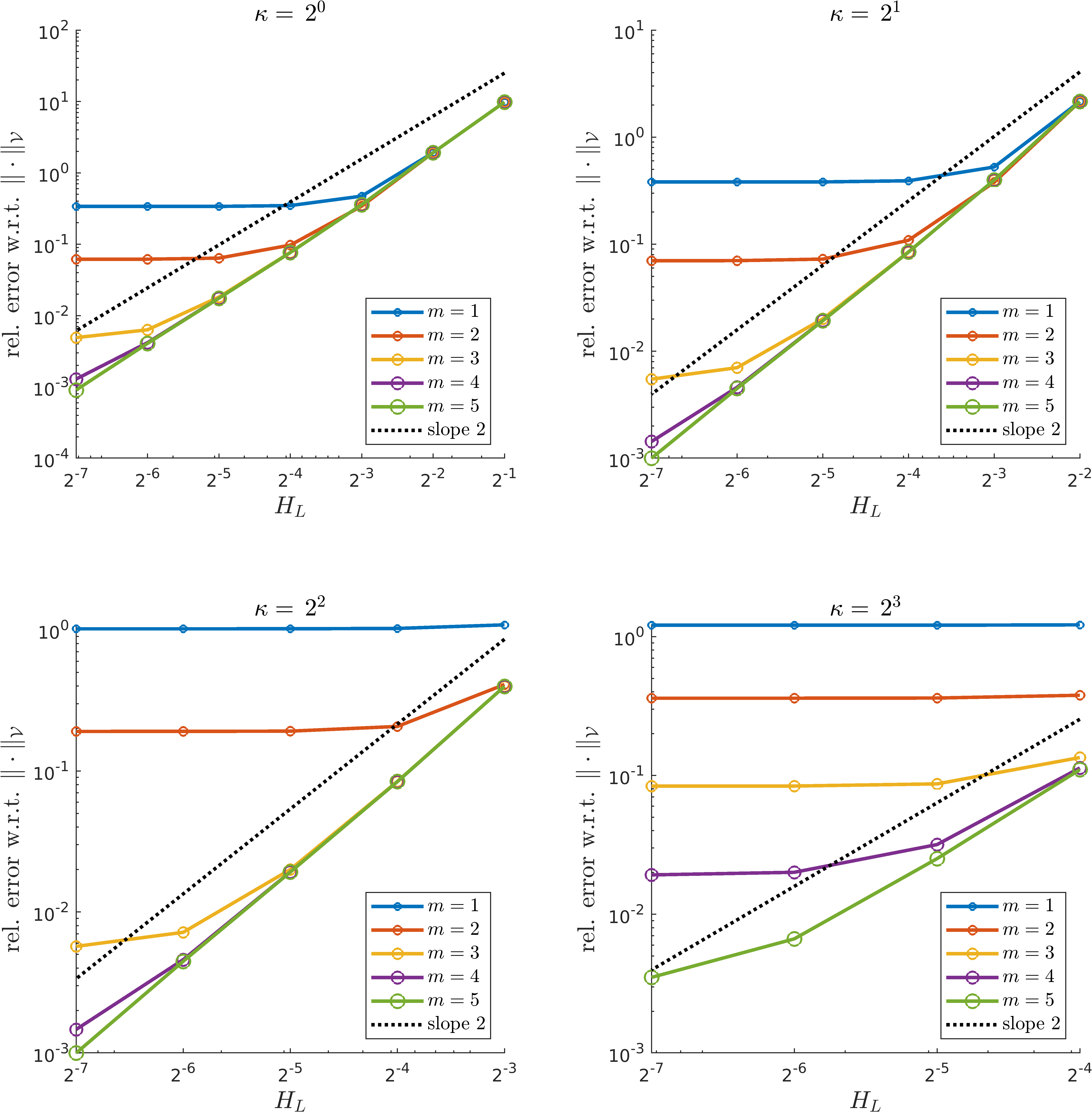
Refer to caption
Figure 8.1. Convergence plots of the proposed multi-level LOD method for oversampling parameters m=1,,5𝑚15m=1,...,5. From left ro right, top to bottom: κ=2j,j=0,,3formulae-sequence𝜅superscript2𝑗𝑗03\kappa=2^{j},j=0,...,3. For comparison, a line with slope 2 is indicated.

In the convergence plots of Figure 8.1, one can clearly see the LOD-typical behavior [31] that the error first decreases with order 222 (fH1(D)𝑓superscript𝐻1𝐷f\in H^{1}(D)), until the localization error dominates, then, the overall error stagnates. This is the expected outcome and is in line with Theorem 6.7. For increasing κ𝜅\kappa, one observes that for small oversampling parameters m𝑚m, the error does not decrease, but stays of order 𝒪(1)𝒪1\mathcal{O}(1). In this case, the oversampling parameter does not fulfill condition (6.5) and convergence cannot be expected.

8.2. Improved stability by novel basis construction

A already mentioned in Remark 6.1, the novel basis construction (6.1) (henceforth referred to as stabilized gamblets) has superior stability properties compared to previously known constructions (henceforth referred to as normal gamblets); see [34, 33, 27]. Since this is true even for the elliptic case, we use the Poisson problem for demonstration purposes

ΔuΔ𝑢\displaystyle-\Delta u =f in D,absent𝑓 in 𝐷\displaystyle=f\qquad\text{ in }D,
u𝑢\displaystyle u =0 on D.absent0 on 𝐷\displaystyle=0\qquad\text{ on }\partial D.

For the numerical experiment, we set D:=(0,1)2assign𝐷superscript012D:=(0,1)^{2} and use the source (8.1). For the sake of simplicity, we consider a single-level method (L=1𝐿1L=1) for demonstrating the improved stability properties. For the multi-level method, the observed phenomena are qualitatively the same. We compute numerical approximations for H1=HL=23,,27formulae-sequencesubscript𝐻1subscript𝐻𝐿superscript23superscript27H_{1}=H_{L}=2^{-3},...,2^{-7} and calculate correctors on a fine mesh with mesh size h=29superscript29h=2^{-9}. Errors are calculated to the reference solution on the same fine mesh.

* Refer to caption
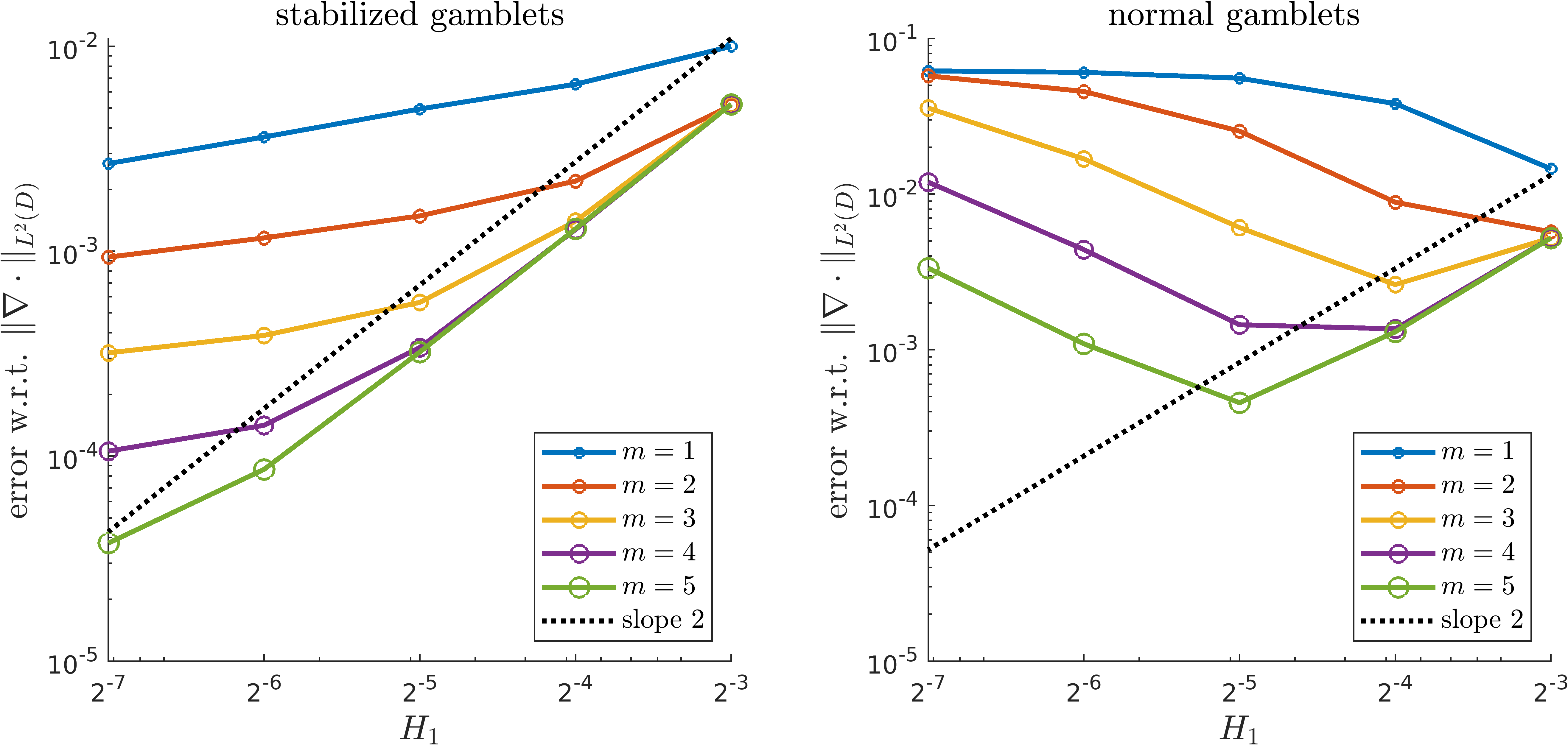
Figure 8.2. Convergence plots of the single-level method for the Poisson problem for oversampling parameters m=1,,5𝑚15m=1,...,5. Left: Stabilized gamblets with improved stability properties; Right: Normal gamblets. For comparison, a line with slope 2 is indicated.

In Figure 8.2, one clearly observes the improved stability properties of stabilized gamblets (6.1) compared to normal gamblets. The error for normal gamblets increases as H1subscript𝐻1H_{1} decreases. Thus, in order to preserve stability, the oversampling parameter m𝑚m has to be increased as the mesh is refined. However, this is not true for the stabilized gamblets, where we have stability for a fixed oversampling parameter. The error even decreases further with a smaller order. This can be explained by the absence of the block-diagonalization error (c.f. Remark 6.3) in the single-level case.

For comparison, we also performed this numerical experiment for the Helmholtz problem with κ=23𝜅superscript23\kappa=2^{3} and Robin-type boundary conditions. Here, the exact same phenomena can be observed; see Figure 8.3.
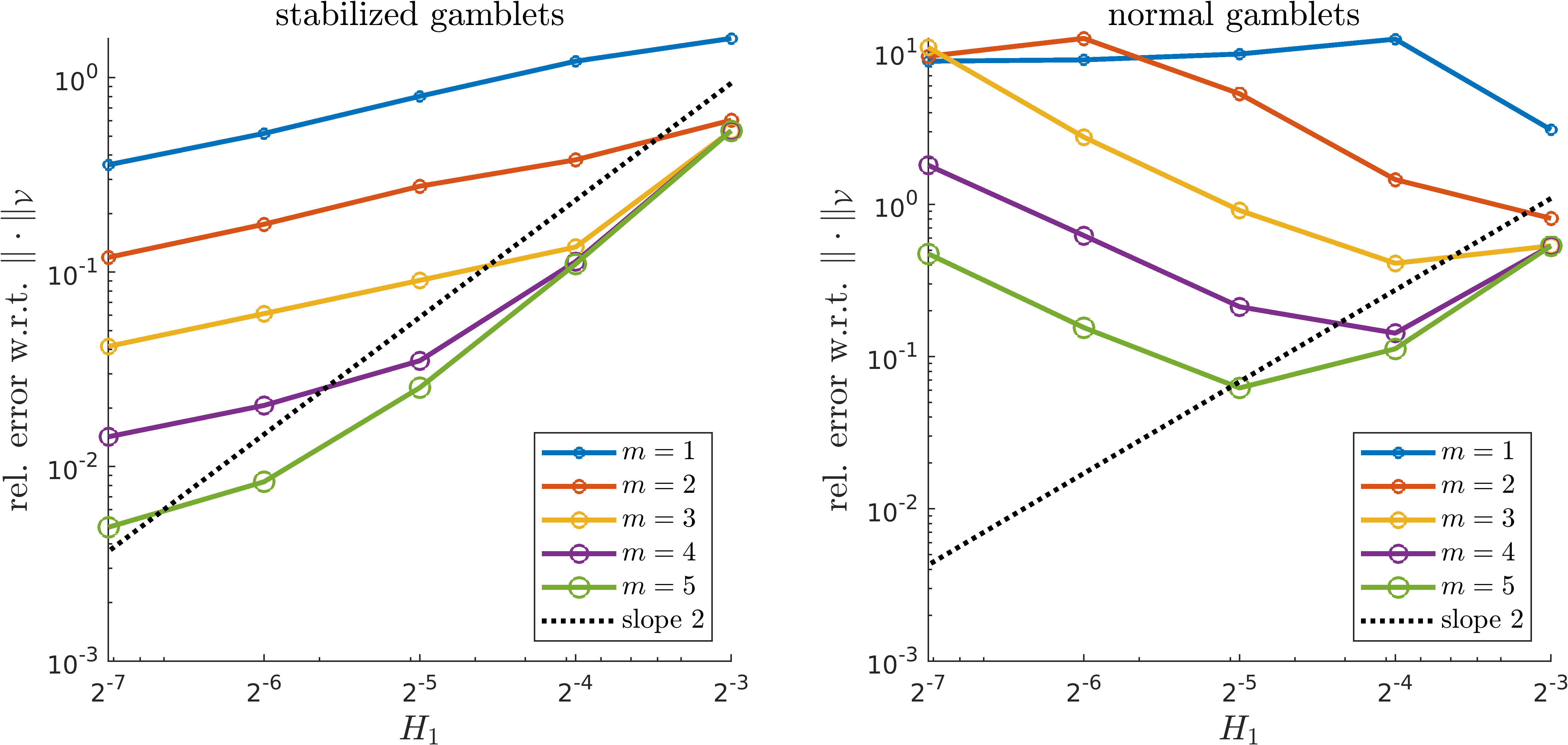
Refer to caption
Figure 8.3. Convergence plots of the single-level method for the Helmholtz problem for oversampling parameters m=1,,5𝑚15m=1,...,5. Left: Stabilized gamblets with improved stability properties; Right: Normal gamblets. For comparison, a line with slope 2 is indicated.

8.3. Variable coefficient

Let us consider the Helmholtz problem in heterogeneous media

(8.2) (Au)κ2u=f𝐴𝑢superscript𝜅2𝑢𝑓-\nabla\cdot(A\nabla u)-\kappa^{2}u=f

with a scalar coefficient AL(D)𝐴superscript𝐿𝐷A\in L^{\infty}(D) satisfying 0<γA(x)γ<0𝛾𝐴𝑥superscript𝛾0<\gamma\leq A(x)\leq\gamma^{\prime}<\infty for almost all xD𝑥𝐷x\in D.

For the numerical experiment, we choose D:=(0,1)2assign𝐷superscript012D:=(0,1)^{2} with ΓR:=DassignsubscriptΓR𝐷\Gamma_{\mathrm{R}}:=\partial D and define for j2𝑗superscript2j\in\mathbb{Z}^{2} and the parameter ϵ=27italic-ϵsuperscript27\epsilon=2^{-7} the inclusions

Sϵj:=ϵ(j+(0.25,0.75)2).assignsuperscriptsubscript𝑆italic-ϵ𝑗italic-ϵ𝑗superscript0.250.752S_{\epsilon}^{j}:=\epsilon\left(j+(0.25,0.75)^{2}\right).

On each inclusion in D𝐷D, the coefficient A𝐴A is chosen to be constant with value uniformly distributed in [1,16]116[1,16]. Everywhere else, A𝐴A is set to 111. For the numerical experiment, we used the realization of A𝐴A shown in Figure 8.4. Since A|D=1evaluated-at𝐴𝐷1A|_{\partial D}=1, this choice is compatible with the Robin boundary conditions from (2.1). The right-hand side is chosen as

(8.3) f(x)={10000exp(11(|xx0|r)2) if |xx0|<r,0 else𝑓𝑥cases1000011superscript𝑥subscript𝑥0𝑟2 if 𝑥subscript𝑥0𝑟0 else\displaystyle f(x)=\begin{cases}10000\,\exp\Big{(}\frac{1}{1-\left(\frac{|x-x_{0}|}{r}\right)^{2}}\Big{)}&\quad\text{ if }\;|x-x_{0}|<r,\\ 0&\quad\text{ else }\end{cases}

with r=0.125𝑟0.125r=0.125 and x0=(0.5,0.5)Tsubscript𝑥0superscript0.50.5𝑇x_{0}=(0.5,0.5)^{T}. In this example, we consider κ=23𝜅superscript23\kappa=2^{3}. Note that the effective wave number in the inclusions is actually smaller than κ𝜅\kappa. As fixed coarse mesh, we use a Cartesian mesh with H1=23subscript𝐻1superscript23H_{1}=2^{-3}. The numerical computations are performed for hierarchy of meshes with HL=23,,27subscript𝐻𝐿superscript23superscript27H_{L}=2^{-3},...,2^{-7}. The correctors are computed on a fine mesh with h=29superscript29h=2^{-9}. Errors are computed to the reference solution on the same fine mesh. As norm for the errors, we choose
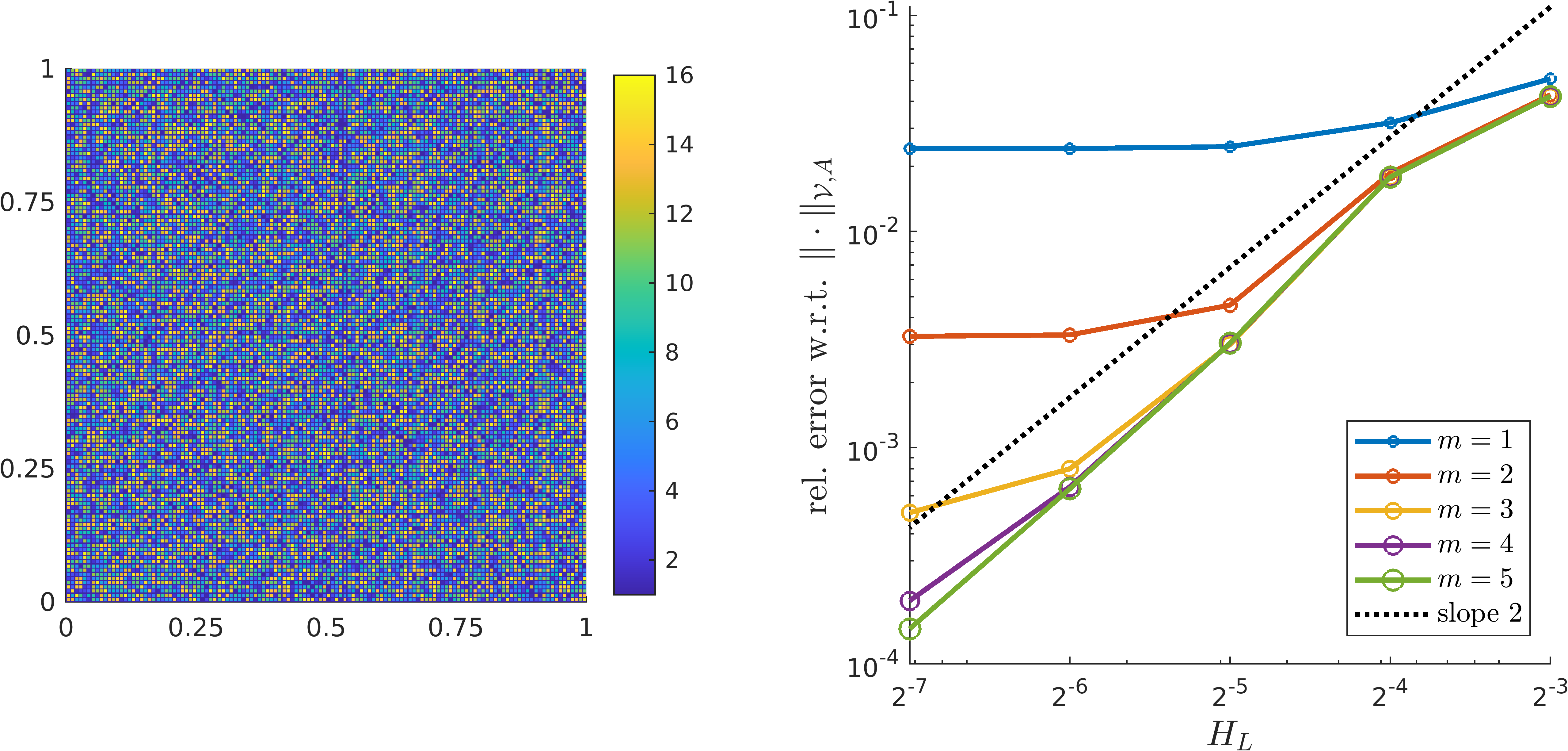
u𝒱,A:=A1/2uL2(D)2+κ2uL2(D)2.assignsubscriptnorm𝑢𝒱𝐴superscriptsubscriptdelimited-∥∥superscript𝐴12𝑢superscript𝐿2𝐷2superscript𝜅2superscriptsubscriptdelimited-∥∥𝑢superscript𝐿2𝐷2\|u\|_{\mathcal{V},A}:=\sqrt{{\left\lVert A^{1/2}\nabla u\right\rVert}_{L^{2}(D)}^{2}+\kappa^{2}{\left\lVert u\right\rVert}_{L^{2}(D)}^{2}}.
Refer to caption
Figure 8.4. Left: Visualization of the realization of A𝐴A used for the numerical experiment. Right: Convergence plot of the LOD method for oversampling parameters m=1,,5𝑚15m=1,...,5. For comparison, a line with slope 2 is indicated.

In Figure 8.4, one observes a convergence behavior similar as in Figure 8.1. In contrast to the convergence test for κ=23𝜅superscript23\kappa=2^{3} in Figure 8.1, the oversampling parameter m=2𝑚2m=2 already yields a good approximation in this example. This can be explained by the smaller effective wave number, caused by the coefficient A𝐴A.

8.4. High-frequency

In this numerical experiment, we again choose D:=(0,1)2assign𝐷superscript012D:=(0,1)^{2} with pure Robin boundary conditions, i.e., ΓR:=DassignsubscriptΓR𝐷\Gamma_{\mathrm{R}}:=\partial D. We consider the wave number κ=26𝜅superscript26\kappa=2^{6} and use the right-hand side (8.3) with the same parameters as in the previous experiment. As fixed coarse mesh, we use a Cartesian mesh with H1=26subscript𝐻1superscript26H_{1}=2^{-6}. The numerical computations are performed for hierarchy of meshes with HL=26,,28subscript𝐻𝐿superscript26superscript28H_{L}=2^{-6},...,2^{-8}. The correctors are computed on a fine mesh with h=210superscript210h=2^{-10}. Errors are computed to the reference solution on the same fine mesh.
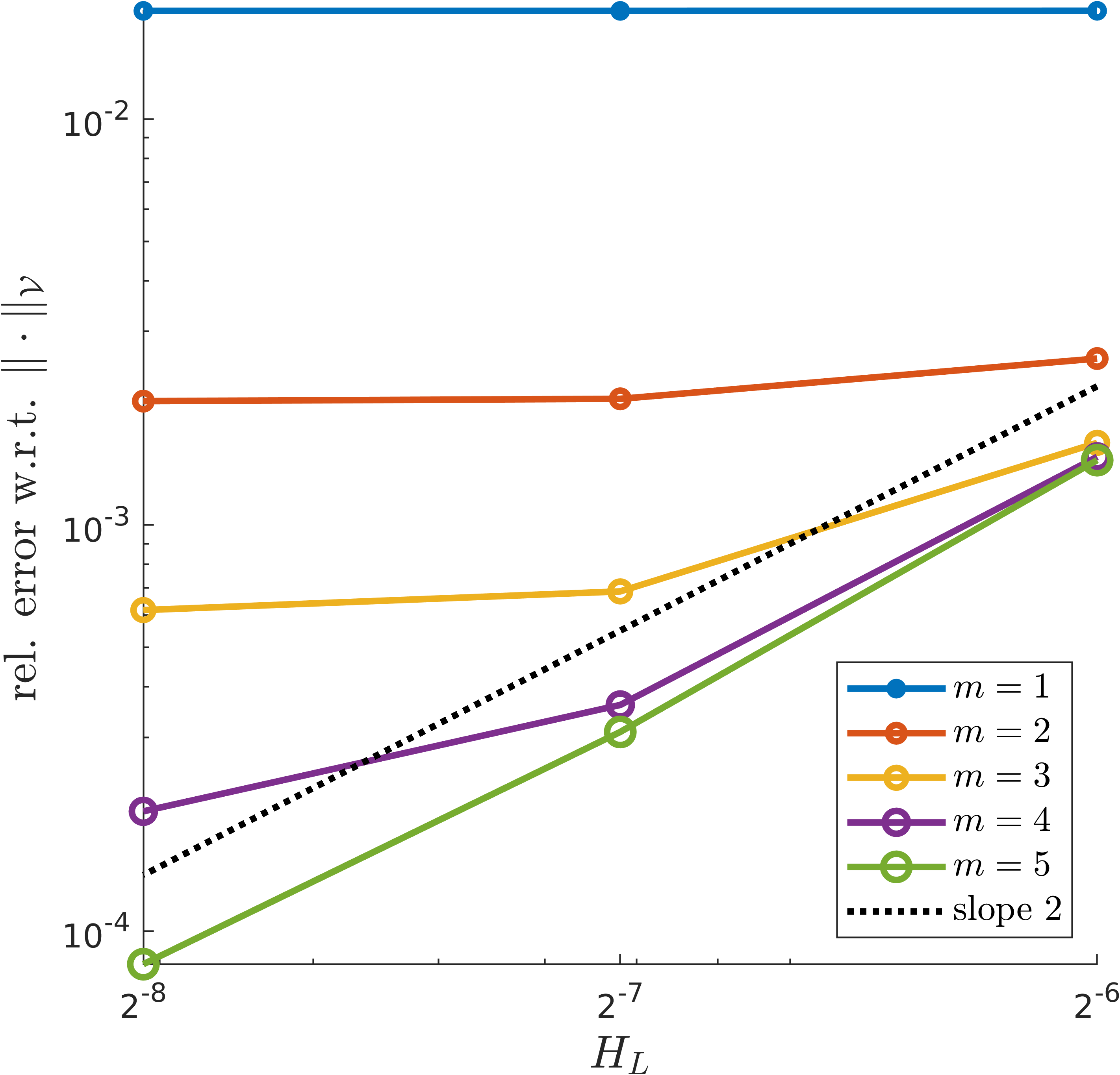
Refer to caption
Figure 8.5. Convergence plots of the proposed multi-level LOD method for the high-frequency example with κ=26𝜅superscript26\kappa=2^{6} for oversampling parameters m=1,,5𝑚15m=1,...,5. For comparison, a line with slope 2 is indicated.

In Figure 8.5 one can observe the convergence behavior as expected from Theorem 6.7, i.e., if the oversampling parameter m𝑚m is chosen sufficiently large (i.e., mlog(κ)greater-than-or-equivalent-to𝑚𝜅m\gtrsim\log(\kappa)), one has κ𝜅\kappa-independent convergence of the proposed multi-resolution method. This numerical example proves the effectiveness of the numerical method also for the high-frequency regime.

8.5. Uniform number of GMRES steps

We consider D:=(0,1)2\Sassign𝐷\superscript012𝑆D:=(0,1)^{2}\backslash S with the scatterer S=[0.375,0.625]2𝑆superscript0.3750.6252S=[0.375,0.625]^{2}. At the boundary of S𝑆S, we impose Dirichlet boundary conditions ΓD=SsubscriptΓD𝑆\Gamma_{\mathrm{D}}=\partial S and Robin boundary conditions are imposed at the artificial boundary ΓR:=D\SassignsubscriptΓR\𝐷𝑆\Gamma_{\mathrm{R}}:=\partial D\backslash\partial S. We use the source (8.3) from above with r=0.05𝑟0.05r=0.05 and x0=(0.125,0.125)subscript𝑥00.1250.125x_{0}=(0.125,0.125). We choose κ=25𝜅superscript25\kappa=2^{5}. The hierarchy used for the computations is specified in Figure 8.6. The correctors are computed on a fine mesh with h=210superscript210h=2^{-10}. The oversampling parameter is chosen as m=2𝑚2m=2. We use the GMRES method with restart after 505050 iterations. The GMRES iteration terminates if a relative residual of 106superscript10610^{-6} is reached.

Refer to caption
Figure 8.6. Table with properties of the linear system of equations for levels =1,,515\ell=1,...,5.

The table in Figure 8.6 clearly shows that uniform boundedness of the number of GMRES iterations for 11\ell\geq 1. As expected, the GMRES iterations performs very poorly for =11\ell=1, which suggests to use a direct solver for the relatively small linear system of equations corresponding to =11\ell=1. The respective condition numbers, which are a good indicator for how fast iterative solvers converge, underline this observation.

References

  • AHP [21] R. Altmann, P. Henning, and D. Peterseim. Numerical homogenization beyond scale separation. Acta Numerica, 30:1–86, 2021.
  • Alp [93] B. Alpert. A class of bases in L2superscript𝐿2{L}^{2} for the sparse representations of integral operators. Siam Journal on Mathematical Analysis, 24:246–262, 1993.
  • BCWG+ [11] T. Betcke, S. N. Chandler-Wilde, I. G. Graham, S. Langdon, and M. Lindner. Condition number estimates for combined potential integral operators in acoustics and their boundary element discretisation. Numerical Methods for Partial Differential Equations, 27(1):31–69, January 2011. Conference on Mathematics of Finite Elements and Applications, 9-12 June 2009, London.
  • BG [16] D. Brown and D. Gallistl. Multiscale sub-grid correction method for time-harmonic high-frequency elastodynamics with wavenumber explicit bounds. Technical report, ArXiv e-print, 1608.04243, 2016.
  • BGP [17] D. L. Brown, D. Gallistl, and D. Peterseim. Multiscale Petrov-Galerkin method for high-frequency heterogeneous Helmholtz equations. In Meshfree methods for partial differential equations VIII, volume 115 of Lect. Notes Comput. Sci. Eng., pages 85–115. Springer, Cham, 2017.
  • BS [08] S. C. Brenner and L. R. Scott. The Mathematical Theory of Finite Element Methods, volume 15 of Texts in Applied Mathematics. Springer, New York, third edition, 2008.
  • CFGNT [18] T. Chaumont-Frelet, D. Gallistl, S. Nicaise, and J. Tomezyk. Wavenumber explicit convergence analysis for finite element discretizations of time-harmonic wave propagation problems with perfectly matched layers. HAL preprint hal-01887267, 2018.
  • DPE [12] D. A. Di Pietro and A. Ern. Mathematical Aspects of Discontinuous Galerkin Methods. Springer, 2012.
  • EG [17] A. Ern and J.-L. Guermond. Finite element quasi-interpolation and best approximation. ESAIM Math. Model. Numer. Anal. (M2AN), 51(4):1367–1385, 2017.
  • EHMP [19] C. Engwer, P. Henning, A. Målqvist, and D. Peterseim. Efficient implementation of the localized orthogonal decomposition method. Comput. Methods Appl. Mech. Engrg., 350:123–153, 2019.
  • EM [11] S. Esterhazy and J. M. Melenk. On stability of discretizations of the Helmholtz equation. Numerical Analysis of Multiscale Problems, page 285–324, Aug 2011.
  • For [77] M. Fortin. An analysis of the convergence of mixed finite element methods. RAIRO. Anal. numér., pages 341 – 354, 1977.
  • FP [20] M. Feischl and D. Peterseim. Sparse compression of expected solution operators. SIAM J. Numer. Anal., 58(6):3144–3164, 2020.
  • GGS [15] M. J. Gander, I. G. Graham, and E. A. Spence. Applying GMRES to the Helmholtz equation with shifted Laplacian preconditioning: what is the largest shift for which wavenumber-independent convergence is guaranteed? Numerische Mathematik, 131(3):567–614, November 2015.
  • GHV [18] D. Gallistl, P. Henning, and B. Verfürth. Numerical homogenization of 𝐇(curl)𝐇curl{\bf{H}}(\rm curl)-problems. SIAM J. Numer. Anal., 56(3):1570–1596, 2018.
  • GP [15] D. Gallistl and D. Peterseim. Stable multiscale Petrov-Galerkin finite element method for high frequency acoustic scattering. Comput. Methods Appl. Mech. Engrg., 295:1–17, 2015.
  • GPS [19] I. G. Graham, O. R. Pembery, and E. A. Spence. The Helmholtz equation in heterogeneous media: A priori bounds, well-posedness, and resonances. Journal of Differential Equations, 266(6):2869–2923, 2019.
  • GS [19] I. G. Graham and S. A. Sauter. Stability and error analysis for the Helmholtz equation with variable coefficients. Math. Comp. 89 (2020), 105-138, 2019.
  • GZ [19] M. J. Gander and H. Zhang. A class of iterative solvers for the Helmholtz equation: Factorizations, sweeping preconditioners, source transfer, single layer potentials, polarized traces, and optimized Schwarz methods. SIAM Rev., 61(1):3–76, January 2019.
  • Het [07] U. Hetmaniuk. Stability estimates for a class of Helmholtz problems. Communications in Mathematical Sciences - COMMUN MATH SCI, 5, 09 2007.
  • HJ [90] R. A. Horn and C. R. Johnson. Matrix Analysis. Cambridge University Press, 1990.
  • HP [13] P. Henning and D. Peterseim. Oversampling for the multiscale finite element method. Multiscale Model. Simul., 11(4):1149–1175, 2013.
  • HP [21] M. Hauck and D. Peterseim. Super-localization of elliptic multiscale problems. ArXiv e-print, 2107.13211, 2021.
  • KA [03] P. Knabner and L. Angermann. Numerical Methods for Elliptic and Parabolic Partial Differential Equations, volume 44 of Texts in Applied Mathematics. Springer, New York, 1 edition, 2003.
  • LPS [18] G. Li, D. Peterseim, and M. Schedensack. Error analysis of a variational multiscale stabilization for convection-dominated diffusion equations in two dimensions. IMA J. Numer. Anal., 38(3):1229–1253, 2018.
  • LT [20] J. Liesen and P. Tichý. The field of values bound on ideal GMRES. ArXiv e-print, 1211.5969, 2020.
  • Mai [20] R. Maier. Computational Multiscale Methods in Unstructured Heterogeneous Media. PhD thesis, University of Augsburg, Augsburg, 2020.
  • Mai [21] R. Maier. A high-order approach to elliptic multiscale problems with general unstructured coefficients. SIAM Journal on Numerical Analysis, 59(2):1067–1089, 2021.
  • Mel [95] J. M. Melenk. On Generalized Finite Element Methods. PhD thesis, University of Maryland, College Park, 1995.
  • MP [14] A. Målqvist and D. Peterseim. Localization of elliptic multiscale problems. Math. Comp., 83(290):2583–2603, 2014.
  • MP [20] A. Målqvist and D. Peterseim. Numerical Homogenization by Localized Orthogonal Decomposition, volume 5 of SIAM Spotlights. Society for Industrial and Applied Mathematics (SIAM), Philadelphia, PA, 2020.
  • MV [20] R. Maier and B. Verfürth. Multiscale scattering in nonlinear Kerr-type media. ArXiv e-print 2011.09168, 2020.
  • OS [19] H. Owhadi and C. Scovel. Operator-Adapted Wavelets, Fast Solvers, and Numerical Homogenization: From a Game Theoretic Approach to Numerical Approximation and Algorithm Design. Cambridge Monographs on Applied and Computational Mathematics. Cambridge University Press, 2019.
  • Owh [17] H. Owhadi. Multigrid with rough coefficients and multiresolution operator decomposition from hierarchical information games. SIAM Rev., 59(1):99–149, 2017.
  • OZ [17] H. Owhadi and L. Zhang. Gamblets for opening the complexity-bottleneck of implicit schemes for hyperbolic and parabolic ODEs/PDEs with rough coefficients. J. Comput. Phys., 347:99–128, 2017.
  • Pet [16] D. Peterseim. Variational multiscale stabilization and the exponential decay of fine-scale correctors. In Building Bridges: Connections and Challenges in Modern Approaches to Numerical Partial Differential Equations, pages 341–367. Springer, 2016.
  • Pet [17] D. Peterseim. Eliminating the pollution effect in Helmholtz problems by local subscale correction. Math. Comp., 86(305):1005–1036, 2017.
  • PV [20] D. Peterseim and B. Verfürth. Computational high frequency scattering from high-contrast heterogeneous media. Math. Comp. 89 (2020), 2649-2674, 2020.
  • RN [20] L. G. Ramos and R. Nabben. A two-level shifted laplace preconditioner for Helmholtz problems: Field-of-values analysis and wavenumber-independent convergence. ArXiv e-print, 2006.08750, 2020.
  • Saa [03] Y. Saad. Iterative Methods for Sparse Linear Systems. Other Titles in Applied Mathematics. SIAM, second edition, 2003.
  • Sch [74] A. H. Schatz. An observation concerning Ritz-Galerkin methods with indefinite bilinear forms. Math. Comp., 28:959–962, 1974.
  • ST [18] S. Sauter and C. Torres. Stability estimate for the Helmholtz equation with rapidly jumping coefficients. Z. Angew. Math. Phys. 69, 139 (2018), 2018.
  • Szy [06] D. B. Szyld. The many proofs of an identity on the norm of oblique projections. Numer. Algorithms, 42(3):309–323, 2006.

Appendix A

Proof of Lemma 4.6.

This proof is based on the proof of [37, Theorem 4.4]. Note that (1𝒞L)1superscriptsubscript𝒞𝐿(1-\mathcal{C}_{L}^{*}) is a Fortin operator (as in the theory of mixed methods [12]), since for all u~𝒰~~𝑢~𝒰\tilde{u}\in\widetilde{\mathcal{U}}, v𝒱𝑣𝒱v\in\mathcal{V}

a(u~,(1𝒞L)v)=a(u~,v)a(u~,𝒞Lv)=a(u~,v),𝑎~𝑢1superscriptsubscript𝒞𝐿𝑣𝑎~𝑢𝑣𝑎~𝑢superscriptsubscript𝒞𝐿𝑣𝑎~𝑢𝑣a(\tilde{u},(1-\mathcal{C}_{L}^{*})v)=a(\tilde{u},v)-a(\tilde{u},\mathcal{C}_{L}^{*}v)=a(\tilde{u},v),

where we used (4.1). The continuity of (1𝒞L)1superscriptsubscript𝒞𝐿(1-\mathcal{C}_{L}^{*}) follows with Remark 4.3.

infu~𝒰~supv~𝒱~a(u~,v~)u~𝒱(D)v~𝒱(D)=infu~𝒰~supv𝒱a(u~,(1𝒞L)v)u~𝒱(D)(1𝒞L)v𝒱(D)subscriptinfimum~𝑢~𝒰subscriptsupremum~𝑣~𝒱𝑎~𝑢~𝑣subscriptdelimited-∥∥~𝑢𝒱𝐷subscriptdelimited-∥∥~𝑣𝒱𝐷subscriptinfimum~𝑢~𝒰subscriptsupremum𝑣𝒱𝑎~𝑢1superscriptsubscript𝒞𝐿𝑣subscriptdelimited-∥∥~𝑢𝒱𝐷subscriptdelimited-∥∥1superscriptsubscript𝒞𝐿𝑣𝒱𝐷\displaystyle\inf_{\tilde{u}\in\widetilde{\mathcal{U}}}\sup_{\tilde{v}\in\widetilde{\mathcal{V}}}\frac{\mathfrak{R}a(\tilde{u},\tilde{v})}{{\left\lVert\tilde{u}\right\rVert}_{\mathcal{V}(D)}{\left\lVert\tilde{v}\right\rVert}_{\mathcal{V}(D)}}=\inf_{\tilde{u}\in\widetilde{\mathcal{U}}}\sup_{v\in\mathcal{V}}\frac{\mathfrak{R}a(\tilde{u},(1-\mathcal{C}_{L}^{*})v)}{{\left\lVert\tilde{u}\right\rVert}_{\mathcal{V}(D)}{\left\lVert(1-\mathcal{C}_{L}^{*})v\right\rVert}_{\mathcal{V}(D)}}
infu~𝒰~supv𝒱a(u~,v)u~𝒱(D)v𝒱(D)infu𝒰supv𝒱a(u,v)u𝒱(D)v𝒱(D)α(1).greater-than-or-equivalent-toabsentsubscriptinfimum~𝑢~𝒰subscriptsupremum𝑣𝒱𝑎~𝑢𝑣subscriptdelimited-∥∥~𝑢𝒱𝐷subscriptdelimited-∥∥𝑣𝒱𝐷subscriptinfimum𝑢𝒰subscriptsupremum𝑣𝒱𝑎𝑢𝑣subscriptdelimited-∥∥𝑢𝒱𝐷subscriptdelimited-∥∥𝑣𝒱𝐷greater-than-or-equivalent-tosuperscript𝛼1\displaystyle\gtrsim\inf_{\tilde{u}\in\widetilde{\mathcal{U}}}\sup_{v\in\mathcal{V}}\frac{\mathfrak{R}a(\tilde{u},v)}{{\left\lVert\tilde{u}\right\rVert}_{\mathcal{V}(D)}{\left\lVert v\right\rVert}_{\mathcal{V}(D)}}\geq\inf_{u\in\mathcal{U}}\sup_{v\in\mathcal{V}}\frac{\mathfrak{R}a({u},v)}{{\left\lVert{u}\right\rVert}_{\mathcal{V}(D)}{\left\lVert v\right\rVert}_{\mathcal{V}(D)}}\gtrsim\alpha^{(1)}.

Thus α(2)superscript𝛼2\alpha^{(2)} has the same κ𝜅\kappa-dependence as α(1)superscript𝛼1\alpha^{(1)}, i.e., α(2)α(1)(cstab(κ)κ)1similar-to-or-equalssuperscript𝛼2superscript𝛼1similar-to-or-equalssuperscriptsubscript𝑐stab𝜅𝜅1\alpha^{(2)}\simeq\alpha^{(1)}\simeq(c_{\mathrm{stab}}(\kappa)\kappa)^{-1}. ∎

Proof of Lemma 4.7.

For s=0𝑠0s=0, the proof can also be found in [37, Theorem 4.5]. Due to Galerkin orthogonality, we have that e:=uu~=𝒞Lu𝒲Lassign𝑒𝑢~𝑢subscript𝒞𝐿𝑢subscript𝒲𝐿e:=u-\tilde{u}=\mathcal{C}_{L}u\in\mathcal{W}_{L}. This implies

12e𝒱(D)212superscriptsubscriptdelimited-∥∥𝑒𝒱𝐷2\displaystyle\frac{1}{2}{\left\lVert e\right\rVert}_{\mathcal{V}(D)}^{2} a(e,e)=(f,e)L2(D)=(fΠLf,e)L2(D)absent𝑎𝑒𝑒subscript𝑓𝑒superscript𝐿2𝐷subscript𝑓subscriptΠ𝐿𝑓𝑒superscript𝐿2𝐷\displaystyle\leq\mathfrak{R}a(e,e)=\mathfrak{R}{\left(f\,,\,e\right)}_{L^{2}(D)}=\mathfrak{R}{\left(f-\Pi_{L}f\,,\,e\right)}_{L^{2}(D)}
fΠLfL2(D)(1ΠL)eL2(D)π1HLfΠLfL2(D)e𝒱(D).absentsubscriptdelimited-∥∥𝑓subscriptΠ𝐿𝑓superscript𝐿2𝐷subscriptdelimited-∥∥1subscriptΠ𝐿𝑒superscript𝐿2𝐷superscript𝜋1subscript𝐻𝐿subscriptdelimited-∥∥𝑓subscriptΠ𝐿𝑓superscript𝐿2𝐷subscriptdelimited-∥∥𝑒𝒱𝐷\displaystyle\leq{\left\lVert f-\Pi_{L}f\right\rVert}_{L^{2}(D)}{\left\lVert(1-\Pi_{L})e\right\rVert}_{L^{2}(D)}\leq\pi^{-1}H_{L}{\left\lVert f-\Pi_{L}f\right\rVert}_{L^{2}(D)}{\left\lVert e\right\rVert}_{\mathcal{V}(D)}.

If fH1(D)𝑓superscript𝐻1𝐷f\in H^{1}(D), then (3.1) yields an additional order in HLsubscript𝐻𝐿H_{L}. Dividing by e𝒱(D)subscriptdelimited-∥∥𝑒𝒱𝐷{\left\lVert e\right\rVert}_{\mathcal{V}(D)}, the result follows for s{0,1}𝑠01s\in\{0,1\}. By arguments from interpolation theory (see e.g. [6]), the assertion can be concluded for any s[0,1]𝑠01s\in[0,1] with a non-explicit constant c𝑐c.

Proof of Lemma 5.2.

Let {1,,L}1𝐿\ell\in\{1,...,L\} be fixed. For shorter notation denote φ:=𝒞,Tvassign𝜑subscript𝒞𝑇𝑣\varphi:=\mathcal{C}_{\ell,T}v. Define the finite element cut-off function ηW1,(D,[0,1])𝜂superscript𝑊1𝐷01\eta\in W^{1,\infty}(D,[0,1]) such that

η0𝜂0\displaystyle\eta\equiv 0\quad in Nm1(T),in superscriptsubscript𝑁𝑚1𝑇\displaystyle\text{ in }N_{\ell}^{m-1}(T),
η1𝜂1\displaystyle\eta\equiv 1\quad in D\Nm(T),\in 𝐷superscriptsubscript𝑁𝑚𝑇\displaystyle\text{ in }D\backslash N_{\ell}^{m}(T),
0η10𝜂1\displaystyle 0\leq\eta\leq 1\qquad in R:=Nm(T)\Nm1(T).assignin 𝑅\superscriptsubscript𝑁𝑚𝑇superscriptsubscript𝑁𝑚1𝑇\displaystyle\text{ in }R:=N_{\ell}^{m}(T)\backslash N_{\ell}^{m-1}(T).

with ηL(D)H1subscriptnorm𝜂superscript𝐿𝐷superscriptsubscript𝐻1\|\nabla\eta\|_{L^{\infty}(D)}\leq H_{\ell}^{-1}. We estimate

φL2(D\Nm(T))2superscriptsubscriptdelimited-∥∥𝜑superscript𝐿2\𝐷superscriptsubscript𝑁𝑚𝑇2\displaystyle{\left\lVert\nabla\varphi\right\rVert}_{L^{2}(D\backslash N_{\ell}^{m}(T))}^{2} =(φ,φ)L2(D\Nm(T))(φ,ηφ)L2(D)absentsubscript𝜑𝜑superscript𝐿2\𝐷superscriptsubscript𝑁𝑚𝑇subscript𝜑𝜂𝜑superscript𝐿2𝐷\displaystyle=\mathfrak{R}{\left(\nabla\varphi\,,\,\nabla\varphi\right)}_{L^{2}(D\backslash N_{\ell}^{m}(T))}\leq\mathfrak{R}{\left(\nabla\varphi\,,\,\eta\nabla\varphi\right)}_{L^{2}(D)}
=(φ,(ηφ))L2(D)(φ,φη)L2(D)absentsubscript𝜑𝜂𝜑superscript𝐿2𝐷subscript𝜑𝜑𝜂superscript𝐿2𝐷\displaystyle=\mathfrak{R}{\left(\nabla\varphi\,,\,\nabla(\eta\varphi)\right)}_{L^{2}(D)}-\mathfrak{R}{\left(\nabla\varphi\,,\,\varphi\nabla\eta\right)}_{L^{2}(D)}
|(φ,(ηφΠ~Π(ηφ)))L2(D)|absentsubscript𝜑𝜂𝜑subscript~ΠsubscriptΠ𝜂𝜑superscript𝐿2𝐷\displaystyle\leq\Big{|}\mathfrak{R}{\left(\nabla\varphi\,,\,\nabla(\eta\varphi-\widetilde{\Pi}_{\ell}\Pi_{\ell}(\eta\varphi))\right)}_{L^{2}(D)}\Big{|}
+|(φ,Π~Π(ηφ))L2(D)|+|(φ,φη)L2(D)|subscript𝜑subscript~ΠsubscriptΠ𝜂𝜑superscript𝐿2𝐷subscript𝜑𝜑𝜂superscript𝐿2𝐷\displaystyle\qquad+\Big{|}\mathfrak{R}{\left(\nabla\varphi\,,\,\nabla\widetilde{\Pi}_{\ell}\Pi_{\ell}(\eta\varphi)\right)}_{L^{2}(D)}\Big{|}+\big{|}\mathfrak{R}{\left(\nabla\varphi\,,\,\varphi\nabla\eta\right)}_{L^{2}(D)}\big{|}
=:M1+M2+M3.\displaystyle=:M_{1}+M_{2}+M_{3}.

For M1subscript𝑀1M_{1}, we have w:=(1Π~Π)(ηφ)𝒲assign𝑤1subscript~ΠsubscriptΠ𝜂𝜑subscript𝒲w:=(1-\widetilde{\Pi}_{\ell}\Pi_{\ell})(\eta\varphi)\in\mathcal{W}_{\ell} and w0𝑤0w\equiv 0 in T𝑇T for m1𝑚1m\geq 1, thus aT(φ,w)=0subscript𝑎𝑇𝜑𝑤0a_{T}(\varphi,w)=0. Furthermore it holds Π~Π(ηφ)0subscript~ΠsubscriptΠ𝜂𝜑0\widetilde{\Pi}_{\ell}\Pi_{\ell}(\eta\varphi)\equiv 0 in D\Nm(T)\𝐷superscriptsubscript𝑁𝑚𝑇D\backslash N_{\ell}^{m}(T) since φ𝒲𝜑subscript𝒲\varphi\in\mathcal{W}_{\ell}. Using the definition of the corrector problems (5.1), (3.1) and (3.2), we get

M1subscript𝑀1\displaystyle M_{1} =|(φ,(ηφΠ~Π(ηφ)))L2(D)|absentsubscript𝜑𝜂𝜑subscript~ΠsubscriptΠ𝜂𝜑superscript𝐿2𝐷\displaystyle=\Big{|}\mathfrak{R}{\left(\nabla\varphi\,,\,\nabla(\eta\varphi-\widetilde{\Pi}_{\ell}\Pi_{\ell}(\eta\varphi))\right)}_{L^{2}(D)}\Big{|}
=|κ2(φ,ηφΠ~Π(ηφ))L2(D)|absentsuperscript𝜅2subscript𝜑𝜂𝜑subscript~ΠsubscriptΠ𝜂𝜑superscript𝐿2𝐷\displaystyle=\Big{|}\mathfrak{R}\kappa^{2}{\left(\varphi\,,\,\eta\varphi-\widetilde{\Pi}_{\ell}\Pi_{\ell}(\eta\varphi)\right)}_{L^{2}(D)}\Big{|}
κ2|(φ,ηφ)L2(D)|+κ2|(φ,Π~Π(ηφ))L2(D)|absentsuperscript𝜅2subscript𝜑𝜂𝜑superscript𝐿2𝐷superscript𝜅2subscript𝜑subscript~ΠsubscriptΠ𝜂𝜑superscript𝐿2𝐷\displaystyle\leq\kappa^{2}\big{|}{\left(\varphi\,,\,\eta\varphi\right)}_{L^{2}(D)}\big{|}+\kappa^{2}\Big{|}{\left(\varphi\,,\,\widetilde{\Pi}_{\ell}\Pi_{\ell}(\eta\varphi)\right)}_{L^{2}(D)}\Big{|}
κ2(1Π)φL2(D\Nm1(T))2+κ2(1Π)φL2(R)2absentsuperscript𝜅2superscriptsubscriptdelimited-∥∥1subscriptΠ𝜑superscript𝐿2\𝐷superscriptsubscript𝑁𝑚1𝑇2superscript𝜅2superscriptsubscriptdelimited-∥∥1subscriptΠ𝜑superscript𝐿2𝑅2\displaystyle\leq\kappa^{2}{\left\lVert(1-\Pi_{\ell})\varphi\right\rVert}_{L^{2}(D\backslash N_{\ell}^{m-1}(T))}^{2}+\kappa^{2}{\left\lVert(1-\Pi_{\ell})\varphi\right\rVert}_{L^{2}(R)}^{2}
π2(κH)2φL2(D\Nm1(T))2+π2(κH)2φL2(R)2absentsuperscript𝜋2superscript𝜅subscript𝐻2superscriptsubscriptdelimited-∥∥𝜑superscript𝐿2\𝐷superscriptsubscript𝑁𝑚1𝑇2superscript𝜋2superscript𝜅subscript𝐻2superscriptsubscriptdelimited-∥∥𝜑superscript𝐿2𝑅2\displaystyle\leq\pi^{-2}(\kappa H_{\ell})^{2}{\left\lVert\nabla\varphi\right\rVert}_{L^{2}(D\backslash N_{\ell}^{m-1}(T))}^{2}+\pi^{-2}(\kappa H_{\ell})^{2}{\left\lVert\nabla\varphi\right\rVert}_{L^{2}(R)}^{2}
12φL2(D\Nm(T))2+12φL2(R)2,absent12superscriptsubscriptdelimited-∥∥𝜑superscript𝐿2\𝐷superscriptsubscript𝑁𝑚𝑇212superscriptsubscriptdelimited-∥∥𝜑superscript𝐿2𝑅2\displaystyle\leq\frac{1}{2}{\left\lVert\nabla\varphi\right\rVert}_{L^{2}(D\backslash N_{\ell}^{m}(T))}^{2}+\frac{1}{2}{\left\lVert\nabla\varphi\right\rVert}_{L^{2}(R)}^{2},

where we used Assumption 4.1. The left term can be absorbed into φL2(D\Nm(T))2superscriptsubscriptdelimited-∥∥𝜑superscript𝐿2\𝐷superscriptsubscript𝑁𝑚𝑇2{\left\lVert\nabla\varphi\right\rVert}_{L^{2}(D\backslash N_{\ell}^{m}(T))}^{2}.
Using that Π~Π(ηφ)0subscript~ΠsubscriptΠ𝜂𝜑0\widetilde{\Pi}_{\ell}\Pi_{\ell}(\eta\varphi)\equiv 0 in D\Nm(T)\𝐷superscriptsubscript𝑁𝑚𝑇D\backslash N_{\ell}^{m}(T), (3.1) and (3.2), we obtain for M2subscript𝑀2M_{2}

M2subscript𝑀2\displaystyle M_{2} =|(φ,Π~Π(ηφ))L2(D)|cinvH1φL2(R)ηφL2(R)absentsubscript𝜑subscript~ΠsubscriptΠ𝜂𝜑superscript𝐿2𝐷subscript𝑐invsuperscriptsubscript𝐻1subscriptdelimited-∥∥𝜑superscript𝐿2𝑅subscriptdelimited-∥∥𝜂𝜑superscript𝐿2𝑅\displaystyle=\Big{|}\mathfrak{R}{\left(\nabla\varphi\,,\,\nabla\widetilde{\Pi}_{\ell}\Pi_{\ell}(\eta\varphi)\right)}_{L^{2}(D)}\Big{|}\leq c_{\mathrm{inv}}H_{\ell}^{-1}{\left\lVert\nabla\varphi\right\rVert}_{L^{2}(R)}{\left\lVert\eta\varphi\right\rVert}_{L^{2}(R)}
cinvH1φL2(R)(1Π)φL2(R)cinvπ1φL2(R)2.absentsubscript𝑐invsuperscriptsubscript𝐻1subscriptdelimited-∥∥𝜑superscript𝐿2𝑅subscriptdelimited-∥∥1subscriptΠ𝜑superscript𝐿2𝑅subscript𝑐invsuperscript𝜋1superscriptsubscriptdelimited-∥∥𝜑superscript𝐿2𝑅2\displaystyle\leq c_{\mathrm{inv}}H_{\ell}^{-1}{\left\lVert\nabla\varphi\right\rVert}_{L^{2}(R)}{\left\lVert(1-\Pi_{\ell})\varphi\right\rVert}_{L^{2}(R)}\leq c_{\mathrm{inv}}\pi^{-1}{\left\lVert\nabla\varphi\right\rVert}_{L^{2}(R)}^{2}.

For M3subscript𝑀3M_{3}, we obtain similarly

M3subscript𝑀3\displaystyle M_{3} =|(φ,φη)L2(D)|H1φL2(R)(1Π)φL2(R)π1φL2(R)2.absentsubscript𝜑𝜑𝜂superscript𝐿2𝐷superscriptsubscript𝐻1subscriptdelimited-∥∥𝜑superscript𝐿2𝑅subscriptdelimited-∥∥1subscriptΠ𝜑superscript𝐿2𝑅superscript𝜋1superscriptsubscriptdelimited-∥∥𝜑superscript𝐿2𝑅2\displaystyle=\big{|}\mathfrak{R}{\left(\nabla\varphi\,,\,\varphi\nabla\eta\right)}_{L^{2}(D)}\big{|}\leq H_{\ell}^{-1}{\left\lVert\nabla\varphi\right\rVert}_{L^{2}(R)}{\left\lVert(1-\Pi_{\ell})\varphi\right\rVert}_{L^{2}(R)}\leq\pi^{-1}{\left\lVert\nabla\varphi\right\rVert}_{L^{2}(R)}^{2}.

Combining the estimates for M1subscript𝑀1M_{1}, M2subscript𝑀2M_{2}, and M3subscript𝑀3M_{3}, yields

12φL2(D\Nm(T))2cφL2(R)212superscriptsubscriptdelimited-∥∥𝜑superscript𝐿2\𝐷superscript𝑁𝑚𝑇2𝑐superscriptsubscriptdelimited-∥∥𝜑superscript𝐿2𝑅2\displaystyle\frac{1}{2}{\left\lVert\nabla\varphi\right\rVert}_{L^{2}(D\backslash N^{m}(T))}^{2}\leq c{\left\lVert\nabla\varphi\right\rVert}_{L^{2}(R)}^{2} =cφL2(D\Nm1(T))cφL2(D\Nm(T))2absent𝑐subscriptdelimited-∥∥𝜑superscript𝐿2\𝐷superscript𝑁𝑚1𝑇𝑐superscriptsubscriptdelimited-∥∥𝜑superscript𝐿2\𝐷superscript𝑁𝑚𝑇2\displaystyle=c{\left\lVert\nabla\varphi\right\rVert}_{L^{2}(D\backslash N^{m-1}(T))}-c{\left\lVert\nabla\varphi\right\rVert}_{L^{2}(D\backslash N^{m}(T))}^{2}
(12+c)φL2(D\Nm(T))2absent12𝑐superscriptsubscriptdelimited-∥∥𝜑superscript𝐿2\𝐷superscript𝑁𝑚𝑇2\displaystyle\Leftrightarrow\;\Big{(}\frac{1}{2}+c\Big{)}{\left\lVert\nabla\varphi\right\rVert}_{L^{2}(D\backslash N^{m}(T))}^{2} cφL2(D\Nm1(T))2absent𝑐superscriptsubscriptdelimited-∥∥𝜑superscript𝐿2\𝐷superscript𝑁𝑚1𝑇2\displaystyle\leq c{\left\lVert\nabla\varphi\right\rVert}_{L^{2}(D\backslash N^{m-1}(T))}^{2}
φL2(D\Nm(T))absentsubscriptdelimited-∥∥𝜑superscript𝐿2\𝐷superscript𝑁𝑚𝑇\displaystyle\Leftrightarrow\;{\left\lVert\nabla\varphi\right\rVert}_{L^{2}(D\backslash N^{m}(T))} βφL2(D\Nm1(T)),absent𝛽subscriptdelimited-∥∥𝜑superscript𝐿2\𝐷superscript𝑁𝑚1𝑇\displaystyle\leq\beta{\left\lVert\nabla\varphi\right\rVert}_{L^{2}(D\backslash N^{m-1}(T))},

where β:=c12+c<1assign𝛽𝑐12𝑐1\beta:=\sqrt{\frac{c}{\frac{1}{2}+c}}<1. Iterating this argument, the assertion follows. ∎

For the proof of Lemma 5.4, we infer the intermediate result

Lemma A.1 (Localization error of element-correctors).

If Assumption 4.1 is satisfied, then it holds for all {1,,L}1𝐿\ell\in\{1,...,L\}, T𝒯𝑇subscript𝒯T\in\mathcal{T}_{\ell}, v𝒱𝑣𝒱v\in\mathcal{V} and m𝑚m\in\mathbb{N} that

(𝒞,Tmv𝒞,Tv)L2(D)βm𝒞,TvL2(D),less-than-or-similar-tosubscriptdelimited-∥∥superscriptsubscript𝒞𝑇𝑚𝑣subscript𝒞𝑇𝑣superscript𝐿2𝐷superscript𝛽𝑚subscriptdelimited-∥∥subscript𝒞𝑇𝑣superscript𝐿2𝐷{\left\lVert\nabla(\mathcal{C}_{\ell,T}^{m}v-\mathcal{C}_{\ell,T}v)\right\rVert}_{L^{2}(D)}\lesssim\beta^{m}{\left\lVert\nabla\mathcal{C}_{\ell,T}v\right\rVert}_{L^{2}(D)},

where β𝛽\beta is the constant from Lemma 5.2. An analogous result holds for 𝒞,Tm,𝒞,Tsuperscriptsubscript𝒞𝑇𝑚superscriptsubscript𝒞𝑇\mathcal{C}_{\ell,T}^{m,*}-\mathcal{C}_{\ell,T}^{*}.

Proof.

Let {1,,L}1𝐿\ell\in\{1,...,L\} be fixed. Moreover, let φ:=𝒞,Tvassign𝜑subscript𝒞𝑇𝑣\varphi:=\mathcal{C}_{\ell,T}v and φm:=𝒞,Tmvassignsuperscript𝜑𝑚superscriptsubscript𝒞𝑇𝑚𝑣\varphi^{m}:=\mathcal{C}_{\ell,T}^{m}v and let w𝒲m(T)subscript𝑤superscriptsubscript𝒲𝑚𝑇w_{\ell}\in\mathcal{W}_{\ell}^{m}(T) be arbitrary. We obtain, using Lemma 4.2 and the Galerkin orthogonality

(φmφ)L2(D)2superscriptsubscriptdelimited-∥∥superscript𝜑𝑚𝜑superscript𝐿2𝐷2\displaystyle{\left\lVert\nabla(\varphi^{m}-\varphi)\right\rVert}_{L^{2}(D)}^{2} a(φmφ,φmφ)=a(φmφ,wφ)less-than-or-similar-toabsent𝑎superscript𝜑𝑚𝜑superscript𝜑𝑚𝜑𝑎superscript𝜑𝑚𝜑subscript𝑤𝜑\displaystyle\lesssim\mathfrak{R}a(\varphi^{m}-\varphi,\varphi^{m}-\varphi)=\mathfrak{R}a(\varphi^{m}-\varphi,w_{\ell}-\varphi)
(φmφ)L2(D)(wφ)L2(D).less-than-or-similar-toabsentsubscriptdelimited-∥∥superscript𝜑𝑚𝜑superscript𝐿2𝐷subscriptdelimited-∥∥subscript𝑤𝜑superscript𝐿2𝐷\displaystyle\lesssim{\left\lVert\nabla(\varphi^{m}-\varphi)\right\rVert}_{L^{2}(D)}{\left\lVert\nabla(w_{\ell}-\varphi)\right\rVert}_{L^{2}(D)}.

Define w:=(1Π~Π)(ηφ)assignsubscript𝑤1subscript~ΠsubscriptΠ𝜂𝜑w_{\ell}:=(1-\widetilde{\Pi}_{\ell}\Pi_{\ell})(\eta\varphi) with the finite element cut-off function ηW1,(D,[0,1])𝜂superscript𝑊1𝐷01\eta\in W^{1,\infty}(D,[0,1]) such that

η1𝜂1\displaystyle\eta\equiv 1\quad in Nm1(T),in superscriptsubscript𝑁𝑚1𝑇\displaystyle\text{ in }N_{\ell}^{m-1}(T),
η0𝜂0\displaystyle\eta\equiv 0\quad in D\Nm(T),\in 𝐷superscriptsubscript𝑁𝑚𝑇\displaystyle\text{ in }D\backslash N_{\ell}^{m}(T),
0η10𝜂1\displaystyle 0\leq\eta\leq 1\qquad in R:=Nm(T)\Nm1(T)assignin 𝑅\superscriptsubscript𝑁𝑚𝑇superscriptsubscript𝑁𝑚1𝑇\displaystyle\text{ in }R:=N_{\ell}^{m}(T)\backslash N_{\ell}^{m-1}(T)

and ηL(D)H1subscriptnorm𝜂superscript𝐿𝐷superscriptsubscript𝐻1\|\nabla\eta\|_{L^{\infty}(D)}\leq H_{\ell}^{-1}. Since w𝒲m(T)subscript𝑤superscriptsubscript𝒲𝑚𝑇w_{\ell}\in\mathcal{W}_{\ell}^{m}(T), we obtain

(φmφ)L2(D)subscriptdelimited-∥∥superscript𝜑𝑚𝜑superscript𝐿2𝐷\displaystyle{\left\lVert\nabla(\varphi^{m}-\varphi)\right\rVert}_{L^{2}(D)} (wφ)L2(D)less-than-or-similar-toabsentsubscriptdelimited-∥∥subscript𝑤𝜑superscript𝐿2𝐷\displaystyle\lesssim{\left\lVert\nabla(w_{\ell}-\varphi)\right\rVert}_{L^{2}(D)}
((1Π~Π)(1η)φ)L2(D\Nm1(T))less-than-or-similar-toabsentsubscriptnorm1subscript~ΠsubscriptΠ1𝜂𝜑superscript𝐿2\𝐷subscriptsuperscript𝑁𝑚1𝑇\displaystyle\lesssim{\|\nabla((1-\widetilde{\Pi}_{\ell}\Pi_{\ell})(1-\eta)\varphi)\|}_{L^{2}(D\backslash N^{m-1}_{\ell}(T))}
φL2(D\Nm1(T))less-than-or-similar-toabsentsubscriptdelimited-∥∥𝜑superscript𝐿2\𝐷subscriptsuperscript𝑁𝑚1𝑇\displaystyle\lesssim{\left\lVert\nabla\varphi\right\rVert}_{L^{2}(D\backslash N^{m-1}_{\ell}(T))}
βm1φL2(D)less-than-or-similar-toabsentsuperscript𝛽𝑚1subscriptdelimited-∥∥𝜑superscript𝐿2𝐷\displaystyle\lesssim\beta^{m-1}{\left\lVert\nabla\varphi\right\rVert}_{L^{2}(D)}
βmφL2(D),less-than-or-similar-toabsentsuperscript𝛽𝑚subscriptdelimited-∥∥𝜑superscript𝐿2𝐷\displaystyle\lesssim\beta^{m}{\left\lVert\nabla\varphi\right\rVert}_{L^{2}(D)},

where we used that

((1Π~Π)(1η)φ)L2(D\Nm1(T))subscriptnorm1subscript~ΠsubscriptΠ1𝜂𝜑superscript𝐿2\𝐷subscriptsuperscript𝑁𝑚1𝑇\displaystyle{\|\nabla((1-\widetilde{\Pi}_{\ell}\Pi_{\ell})(1-\eta)\varphi)\|}_{L^{2}(D\backslash N^{m-1}_{\ell}(T))}
((1η)φ)L2(D\Nm1(T))+H1(1η)φL2(D\Nm1(T))less-than-or-similar-toabsentsubscriptdelimited-∥∥1𝜂𝜑superscript𝐿2\𝐷subscriptsuperscript𝑁𝑚1𝑇superscriptsubscript𝐻1subscriptdelimited-∥∥1𝜂𝜑superscript𝐿2\𝐷subscriptsuperscript𝑁𝑚1𝑇\displaystyle\quad\lesssim{\left\lVert\nabla((1-\eta)\varphi)\right\rVert}_{L^{2}(D\backslash N^{m-1}_{\ell}(T))}+H_{\ell}^{-1}{\left\lVert(1-\eta)\varphi\right\rVert}_{L^{2}(D\backslash N^{m-1}_{\ell}(T))}
φL2(D\Nm1(T))+φηL2(R)+H1φL2(D\Nm1(T))less-than-or-similar-toabsentsubscriptdelimited-∥∥𝜑superscript𝐿2\𝐷subscriptsuperscript𝑁𝑚1𝑇subscriptdelimited-∥∥𝜑𝜂superscript𝐿2𝑅superscriptsubscript𝐻1subscriptdelimited-∥∥𝜑superscript𝐿2\𝐷subscriptsuperscript𝑁𝑚1𝑇\displaystyle\quad\lesssim{\left\lVert\nabla\varphi\right\rVert}_{L^{2}(D\backslash N^{m-1}_{\ell}(T))}+{\left\lVert\varphi\nabla\eta\right\rVert}_{L^{2}(R)}+H_{\ell}^{-1}{\left\lVert\varphi\right\rVert}_{L^{2}(D\backslash N^{m-1}_{\ell}(T))}
φL2(D\Nm1(T)).less-than-or-similar-toabsentsubscriptdelimited-∥∥𝜑superscript𝐿2\𝐷subscriptsuperscript𝑁𝑚1𝑇\displaystyle\quad\lesssim{\left\lVert\nabla\varphi\right\rVert}_{L^{2}(D\backslash N^{m-1}_{\ell}(T))}.

Here, we applied (3.1) and (3.2) multiple times. ∎

Proof of Lemma 5.4.

Let {1,..,L}\ell\in\{1,..,L\} be fixed. Define z:=𝒞mv𝒞vassign𝑧superscriptsubscript𝒞𝑚𝑣subscript𝒞𝑣z:=\mathcal{C}_{\ell}^{m}v-\mathcal{C}_{\ell}v and zT=𝒞,Tmv𝒞,Tvsubscript𝑧𝑇superscriptsubscript𝒞𝑇𝑚𝑣subscript𝒞𝑇𝑣z_{T}=\mathcal{C}_{\ell,T}^{m}v-\mathcal{C}_{\ell,T}v for T𝒯𝑇subscript𝒯T\in\mathcal{T}_{\ell}. It holds

zL2(D)2a(z,z)=T𝒯a(zT,z).less-than-or-similar-tosuperscriptsubscriptdelimited-∥∥𝑧superscript𝐿2𝐷2𝑎𝑧𝑧subscript𝑇subscript𝒯𝑎subscript𝑧𝑇𝑧{\left\lVert\nabla z\right\rVert}_{L^{2}(D)}^{2}\lesssim a(z,z)=\sum_{T\in\mathcal{T}_{\ell}}a(z_{T},z).

For T𝒯𝑇subscript𝒯T\in\mathcal{T}_{\ell} define finite element the cut-off function ηW1,(D,[0,1])𝜂superscript𝑊1𝐷01\eta\in W^{1,\infty}(D,[0,1]) such that

η0𝜂0\displaystyle\eta\equiv 0\quad in Nm(T),in superscriptsubscript𝑁𝑚𝑇\displaystyle\text{ in }N_{\ell}^{m}(T),
η1𝜂1\displaystyle\eta\equiv 1\quad in D\Nm+1(T),\in 𝐷superscriptsubscript𝑁𝑚1𝑇\displaystyle\text{ in }D\backslash N_{\ell}^{m+1}(T),
0η10𝜂1\displaystyle 0\leq\eta\leq 1\qquad in R:=Nm+1(T)\Nm(T)assignin 𝑅\superscriptsubscript𝑁𝑚1𝑇superscriptsubscript𝑁𝑚𝑇\displaystyle\text{ in }R:=N_{\ell}^{m+1}(T)\backslash N_{\ell}^{m}(T)

and ηL(D)H1subscriptnorm𝜂superscript𝐿𝐷superscriptsubscript𝐻1\|\nabla\eta\|_{L^{\infty}(D)}\leq H_{\ell}^{-1}. Using supp((1Π~Π)(ηz))D\Nm(T)supp1subscript~ΠsubscriptΠ𝜂𝑧\𝐷superscriptsubscript𝑁𝑚𝑇\mathrm{supp}((1-\widetilde{\Pi}_{\ell}\Pi_{\ell})(\eta z))\subset D\backslash N_{\ell}^{m}(T), (1Π~Π)(ηz)W1subscript~ΠsubscriptΠ𝜂𝑧subscript𝑊(1-\widetilde{\Pi}_{\ell}\Pi_{\ell})(\eta z)\in W_{\ell}, and (5.1), we get

a(zT,(1Π~Π)(ηz))=a(𝒞,Tv,(1Π~Π)(ηz))=0.𝑎subscript𝑧𝑇1subscript~ΠsubscriptΠ𝜂𝑧𝑎subscript𝒞𝑇𝑣1subscript~ΠsubscriptΠ𝜂𝑧0a(z_{T},(1-\widetilde{\Pi}_{\ell}\Pi_{\ell})(\eta z))=-a(\mathcal{C}_{\ell,T}v,(1-\widetilde{\Pi}_{\ell}\Pi_{\ell})(\eta z))=0.

Hence, using that z=(1Π~Π)z𝑧1subscript~ΠsubscriptΠ𝑧z=(1-\widetilde{\Pi}_{\ell}\Pi_{\ell})z, yields

a(zT,z)=a(zT,z(1Π~Π)(ηz))=a(zT,(1Π~Π)((1η)z)).𝑎subscript𝑧𝑇𝑧𝑎subscript𝑧𝑇𝑧1subscript~ΠsubscriptΠ𝜂𝑧𝑎subscript𝑧𝑇1subscript~ΠsubscriptΠ1𝜂𝑧a(z_{T},z)=a(z_{T},z-(1-\widetilde{\Pi}_{\ell}\Pi_{\ell})(\eta z))=a(z_{T},(1-\widetilde{\Pi}_{\ell}\Pi_{\ell})((1-\eta)z)).

With (3.1) and (3.2), one obtains the bound

|a(zT,(1Π~Π)((1η)z))|zT𝒱(D)z𝒱(Nm+1(T)).less-than-or-similar-to𝑎subscript𝑧𝑇1subscript~ΠsubscriptΠ1𝜂𝑧subscriptdelimited-∥∥subscript𝑧𝑇𝒱𝐷subscriptdelimited-∥∥𝑧𝒱superscriptsubscript𝑁𝑚1𝑇\big{|}a(z_{T},(1-\widetilde{\Pi}_{\ell}\Pi_{\ell})((1-\eta)z))\big{|}\lesssim{\left\lVert z_{T}\right\rVert}_{\mathcal{V}(D)}{\left\lVert z\right\rVert}_{\mathcal{V}(N_{\ell}^{m+1}(T))}.

The element-correctors satisfy the estimate 𝒞,TvL2(D)v𝒱(T)less-than-or-similar-tosubscriptdelimited-∥∥subscript𝒞𝑇𝑣superscript𝐿2𝐷subscriptdelimited-∥∥𝑣𝒱𝑇{\left\lVert\nabla\mathcal{C}_{\ell,T}v\right\rVert}_{L^{2}(D)}\lesssim{\left\lVert v\right\rVert}_{\mathcal{V}(T)}, since

𝒞,TvL2(D)2a(𝒞,Tv,𝒞,Tv)=aT(v,𝒞,Tv)v𝒱(T)𝒞,TvL2(D).less-than-or-similar-tosuperscriptsubscriptdelimited-∥∥subscript𝒞𝑇𝑣superscript𝐿2𝐷2𝑎subscript𝒞𝑇𝑣subscript𝒞𝑇𝑣subscript𝑎𝑇𝑣subscript𝒞𝑇𝑣less-than-or-similar-tosubscriptdelimited-∥∥𝑣𝒱𝑇subscriptdelimited-∥∥subscript𝒞𝑇𝑣superscript𝐿2𝐷\displaystyle{\left\lVert\nabla\mathcal{C}_{\ell,T}v\right\rVert}_{L^{2}(D)}^{2}\lesssim a(\mathcal{C}_{\ell,T}v,\mathcal{C}_{\ell,T}v)=a_{T}(v,\mathcal{C}_{\ell,T}v)\lesssim{\left\lVert v\right\rVert}_{\mathcal{V}(T)}{\left\lVert\nabla\mathcal{C}_{\ell,T}v\right\rVert}_{L^{2}(D)}.

Using this and Lemma 4.2, Lemma A.1 and the finite overlap of the patches, we get after summing over all elements

zL2(D)2superscriptsubscriptdelimited-∥∥𝑧superscript𝐿2𝐷2\displaystyle{\left\lVert\nabla z\right\rVert}_{L^{2}(D)}^{2} T𝒯a(zT,z)T𝒯zT𝒱(D)z𝒱(Nm+1(T))less-than-or-similar-toabsentsubscript𝑇subscript𝒯𝑎subscript𝑧𝑇𝑧less-than-or-similar-tosubscript𝑇subscript𝒯subscriptdelimited-∥∥subscript𝑧𝑇𝒱𝐷subscriptdelimited-∥∥𝑧𝒱superscriptsubscript𝑁𝑚1𝑇\displaystyle\lesssim\sum_{T\in\mathcal{T}_{\ell}}a(z_{T},z)\lesssim\sum_{T\in\mathcal{T}_{\ell}}{\left\lVert z_{T}\right\rVert}_{\mathcal{V}(D)}{\left\lVert z\right\rVert}_{\mathcal{V}(N_{\ell}^{m+1}(T))}
βmT𝒯𝒞,TvL2(D)z𝒱(Nm+1(T))less-than-or-similar-toabsentsuperscript𝛽𝑚subscript𝑇subscript𝒯subscriptdelimited-∥∥subscript𝒞𝑇𝑣superscript𝐿2𝐷subscriptdelimited-∥∥𝑧𝒱superscriptsubscript𝑁𝑚1𝑇\displaystyle\lesssim\beta^{m}\sum_{T\in\mathcal{T}_{\ell}}{\left\lVert\nabla\mathcal{C}_{\ell,T}v\right\rVert}_{L^{2}(D)}{\left\lVert z\right\rVert}_{\mathcal{V}(N_{\ell}^{m+1}(T))}
βmT𝒯v𝒱(T)z𝒱(Nm+1(T))less-than-or-similar-toabsentsuperscript𝛽𝑚subscript𝑇subscript𝒯subscriptdelimited-∥∥𝑣𝒱𝑇subscriptdelimited-∥∥𝑧𝒱superscriptsubscript𝑁𝑚1𝑇\displaystyle\lesssim\beta^{m}\sum_{T\in\mathcal{T}_{\ell}}{\left\lVert v\right\rVert}_{\mathcal{V}(T)}{\left\lVert z\right\rVert}_{\mathcal{V}(N_{\ell}^{m+1}(T))}
cmβmv𝒱(D)z𝒱(D)cmβmv𝒱(D)zL2(D).less-than-or-similar-toabsentsubscript𝑐𝑚superscript𝛽𝑚subscriptdelimited-∥∥𝑣𝒱𝐷subscriptdelimited-∥∥𝑧𝒱𝐷less-than-or-similar-tosubscript𝑐𝑚superscript𝛽𝑚subscriptdelimited-∥∥𝑣𝒱𝐷subscriptdelimited-∥∥𝑧superscript𝐿2𝐷\displaystyle\lesssim c_{m}\beta^{m}{\left\lVert v\right\rVert}_{\mathcal{V}(D)}{\left\lVert z\right\rVert}_{\mathcal{V}(D)}\lesssim c_{m}\beta^{m}{\left\lVert v\right\rVert}_{\mathcal{V}(D)}{\left\lVert\nabla z\right\rVert}_{L^{2}(D)}.

with constant cmsubscript𝑐𝑚c_{m} depending polynomially on the oversampling parameter m𝑚m. ∎