The X-ray evolution and geometry of the 2018 outburst of XTE  J1810–197

Abstract

After 15 years, in late 2018, the magnetar XTE J1810–197 underwent a second recorded X-ray outburst event and reactivated as a radio pulsar. We initiated an X-ray monitoring campaign to follow the timing and spectral evolution of the magnetar as its flux decays using Swift, XMM–Newton, NuSTAR, and NICER observations. During the year-long campaign, the magnetar reproduced similar behaviour to that found for the first outburst, with a factor of two change in its spin-down rate from $\sim 7.2\times 10^{-12}$ s s^-1 to $\sim 1.5\times 10^{-11}$ s s^-1  after two months. Unique to this outburst, we confirm the peculiar energy-dependent phase shift of the pulse profile. Following the initial outburst, the spectrum of XTE J1810–197 is well-modelled by multiple blackbody components corresponding to a pair of non-concentric, hot thermal caps surrounded by a cooler one, superposed to the colder star surface. We model the energy-dependent pulse profile to constrain the viewing and surface emission geometry and find that the overall geometry of XTE J1810–197 has likely evolved relative to that found for the 2003 event.

Table 1: Log of the X-ray observations of XTE J1810–197 between 2018 December 13 and 2019 October 25.

Obs. ID	Instrument∗	Start time (TT)	Mid Point	Exposure	Source net count rate∗∗
		(YYYY-MM-DD hh:mm:ss)	(MJD)	(ks)	(counts s-1)
90410368002	NuSTAR/FPMA	2018-12-13 03:11:09	58465.587	39.2	1.44(1)
90410368002	NuSTAR/FPMB	2018-12-13 03:11:09	58465.587	39.1	1.44(1)
80202013002	NuSTAR/FPMA	2019-01-02 21:06:09	58486.346	46.0	1.13(1)
80202013002	NuSTAR/FPMB	2019-01-02 21:06:09	58486.346	45.4	1.06(1)
80202013003	NuSTAR/FPMA	2019-02-07 15:31:09	58522.134	40.1	1.17(1)
80202013003	NuSTAR/FMPB	2019-02-07 15:31:09	58522.134	39.7	1.15(1)
00031335006	Swift/XRT (WT)	2019-02-08 19:18:20	58522.843	1.9	3.86(4)
00031335007	Swift/XRT (WT)	2019-02-15 21:51:38	58530.050	4.6	2.95(3)
1020420142	NICER	2019-02-21 02:12:00	58535.258	1.8	46.9(2)
00031335008	Swift/XRT (WT)	2019-02-22 06:42:33	58536.321	2.0	3.09(4)
00031335009	Swift/XRT (WT)	2019-03-02 17:24:50	58544.764	1.5	3.07(5)
80202013005	NuSTAR/FPMA	2019-03-03 22:46:09	58546.405	38.9	0.94(1)
80202013005	NuSTAR/FPMB	2019-03-03 22:46:09	58546.405	38.8	0.91(1)
2618010101a	NICER	2019-03-03 23:52:25	58546.357	7.3	42.7(1)
0784303101	XMM/EPIC-pn (TM)	2019-03-04 02:36:19	58546.183	12.9	29.19(5)
2020420103a	NICER	2019-03-04 18:19:12	58546.8707	4.3	43.3(1)
00031335010†	Swift/XRT (WT)	2019-03-08 05:56:17	58550.279	0.7	2.98(7)
00031335011†	Swift/XRT (WT)	2019-03-13 14:43:05	58555.652	1.5	3.14(5)
00031335012	Swift/XRT (WT)	2019-03-15 22:27:48	58558.441	2.1	3.11(4)
00031335013	Swift/XRT (WT)	2019-03-22 13:41:45	58564.614	1.7	2.93(4)
2020420104	NICER	2019-03-29 19:25:32	58571.856	3.9	39.6(1)
00031335014	Swift/XRT (WT)	2019-03-29 21:03:31	58572.081	2.1	2.89(4)
2020420105b	NICER	2019-03-31 17:47:14	58573.853	7.5	37.5(1)
2020420106b	NICER	2019-03-31 23:58:33	58574.014	2.0	37.6(1)
00031335015‡	Swift/XRT (WT)	2019-04-05 04:25:28	58578.260	1.0	2.14(5)
2020420107	NICER	2019-04-07 13:42:40	58580.618	3.4	36.5(1)
2618010201c	NICER	2019-04-12 16:12:40	58585.812	3.7	36.4(1)
00031335016‡	Swift/XRT (WT)	2019-04-12 21:40:54	58585.932	0.6	2.43(7)
2618010202c	NICER	2019-04-12 23:56:40	58586.167	3.9	36.4(1)
00031335017	Swift/XRT (WT)	2019-04-17 06:41:10	58590.584	1.5	2.69(4)
00031335018	Swift/XRT (WT)	2019-04-19 01:42:46	58592.136	1.9	2.77(4)
00031335021	Swift/XRT (WT)	2019-05-03 13:10:44	58606.585	1.4	2.51(4)
00031335022	Swift/XRT (WT)	2019-05-10 18:47:11	58614.313	1.8	0.48(2)
00031335023	Swift/XRT (WT)	2019-05-17 15:08:39	58620.733	1.6	1.55(3)
2618010301d	NICER	2019-05-23 21:41:40	58626.947	2.8	31.9(1)
2618010302d	NICER	2019-05-24 00:47:40	58627.495	9.9	31.9(1)
00031335024	Swift/XRT (WT)	2019-05-24 18:49:41	58627.819	1.8	2.25(4)
2618010303	NICER	2019-05-25 00:12:00	58628.337	4.1	31.7(1)
00031335025e	Swift/XRT (WT)	2019-05-30 15:02:56	58633.634	0.4	2.25(7)
00031335026e	Swift/XRT (WT)	2019-06-01 19:57:34	58635.904	1.6	1.96(4)
00031335027	Swift/XRT (WT)	2019-06-09 06:18:32	58643.302	1.9	2.16(3)
00031335028f	Swift/XRT (WT)	2019-06-25 17:23:02	58659.729	0.9	1.96(4)
00031335029f	Swift/XRT (WT)	2019-06-26 12:31:41	58660.525	0.6	2.12(6)
00031335031††	Swift/XRT (WT)	2019-06-30 23:43:59	58664.992	0.5	1.94(6)
00031335032††	Swift/XRT (WT)	2019-07-03 12:11:51	58667.513	0.8	1.88(5)
2618010401	NICER	2019-07-07 01:25:30	58671.493	7.9	27.4(1)
00031335034	Swift/XRT (WT)	2019-07-12 04:46:47	58676.272	1.1	1.67(4)
00031335036	Swift/XRT (WT)	2019-07-25 18:14:18	58689.828	1.5	1.14(2)
00031335037	Swift/XRT (WT)	2019-08-01 00:03:15	58696.002	0.9	0.97(3)
2618010501g	NICER	2019-08-05 20:57:40	58700.908	1.0	24.4(2)
2618010502g	NICER	2019-08-06 00:03:20	58701.489	2.9	23.7(1)
2618010503g	NICER	2019-08-07 00:31:47	58702.480	3.5	23.5(1)
2618010504	NICER	2019-08-07 23:42:47	58703.482	6.5	23.6(1)
2618010505	NICER	2019-08-14 01:09:00	58709.215	1.1	23.8(1)
00031335038	Swift/XRT (WT)	2019-08-13 15:54:19	58708.700	1.6	1.74(3)
00031335043	Swift/XRT (PC)	2019-09-17 01:28:53	58743.530	1.2	0.57(2)
2618010601	NICER	2019-09-21 10:18:25	58747.695	6.0	21.3(1)
2618010602	NICER	2019-09-22 00:14:25	58748.308	6.9	21.3(1)
30501023002	NuSTAR/FPMA	2019-09-22 00:16:09	58749.212	95.6	0.45(2)
30501023002	NuSTAR/FPMB	2019-09-22 00:16:09	58749.212	96.1	0.44(2)
0784303201	XMM/EPIC-pn (SW)	2019-09-22 14:52:41	58748.947	56.5	9.49(1)
00031335044	Swift/XRT (PC)	2019-09-25 18:14:20	58751.864	1.6	0.57(2)
30501023004	NuSTAR/FPMA	2019-09-26 21:51:09	58753.481	43.2	0.42(3)
30501023004	NuSTAR/FPMB	2019-09-26 21:51:09	58753.481	43.5	0.41(3)
00031335045	Swift/XRT (PC)	2019-10-06 21:59:58	58762.954	1.6	0.40(2)
00031335046	Swift/XRT (PC)	2019-10-15 00:35:43	58771.098	2.2	0.49(1)
00031335047	Swift/XRT (PC)	2019-10-25 04:21:03	58781.215	1.7	0.47(2)

• The instrumental setup is indicated in brackets: WT = windowed timing, TM = timing mode, PC = photon counting and SW = small window.

• The source net count rate in the 0.3–10 keV range for XMM–Newton and Swift, in the 0.6–7 keV interval for NICER, and in the 3–15 keV range for NuSTAR.

• These observations were merged in the spectral analysis.

• These observations were merged in the timing analysis.

1 Introduction

Magnetars are isolated pulsars whose emission is thought to be powered by the decay and instabilities of their extreme magnetic fields, typically $B$ $\sim$ 10¹⁴–10¹⁵ G (see e.g., Kaspi & Beloborodov, 2017; Esposito et al., 2021, for reviews). With spin periods in the 0.3–12 s range and relatively large spin-down rates, these objects have a persistent X-ray luminosity of $L_{X}$ $\sim$ 10³¹–10³⁶ erg s^-1, generally larger than their rotational energy loss rate. The main feature of these isolated neutron stars is the unpredictable and variable bursting activity in the X-/gamma-ray bands on different time scales. These flaring events often indicate that the source has entered an active phase, commonly referred to as outburst (see the Magnetar Outburst Online Catalog, Coti Zelati et al., 2018). During an outburst, the persistent X-ray flux increases by up to three orders of magnitude above the quiescent level. Then, it usually relaxes back to the pre-outburst level on time scales spanning from weeks to months/years. Up to now, about 30 sources are listed as magnetars, although magnetar-like activity has been recorded from other classes of isolated neutron stars too, such as high-$B$ radio pulsars (e.g., Archibald et al., 2016) and the source at the centre of the supernova remnant RCW 103 (D’Aì et al., 2016; Rea et al., 2016).

XTE J1810–197 (XTE J1810) unveiled its magnetar nature in 2003 when the Rossi X-ray Timing Explorer (RXTE) detected an increase in its X-ray flux by a factor of $\sim$ 100 with respect to the quiescent level measured by ROSAT in 1993, $\sim$5$\times 10^{-13}$ erg s^-1cm^-2 (0.5–10 keV; Ibrahim et al., 2004; Gotthelf et al., 2004). The outburst provided the opportunity to detect the spin signal, at a period of $\sim$ 5.54 s. Archival VLA 1.4 GHz survey data from 2004 January revealed post-outburst radio emission from the magnetar (Halpern et al., 2005) that lead to the discovery in 2006 of radio pulsations at the X-ray spin period (Camilo et al., 2006). XTE J1810 was the first magnetar to show pulsed emission in the radio band. The X-ray flux reached the pre-outburst level in early 2007 (Bernardini et al., 2009; Alford & Halpern, 2016), although the source remained radio loud until late 2008 (Camilo et al., 2016). The initial phases of the outburst were missed, therefore it was not possible to fully characterize the magnetar properties at the outburst peak. XMM–Newton started to monitor XTE J1810 approximately one year after the outburst onset. Spectral and temporal studies during the early decay revealed a variable spin-down rate and a two temperature thermal spectrum, suggesting a localized surface hot spot with temperature of $kT_{\rm hot}$$\sim$0.7 keV surrounded by a cooler corona with $kT_{\rm warm}$$\sim$0.3 keV (see, e.g., Halpern & Gotthelf, 2005, and references therein). These two regions were superimposed on the quiescent component ($kT_{\rm cold}\sim$0.15 keV) which was identified with the thermal emission from the whole neutron star surface (Perna & Gotthelf, 2008; Bernardini et al., 2009; Albano et al., 2010; Alford & Halpern, 2016). An extensive radio and X-ray monitoring allowed to study the timing properties of XTE J1810 over the outburst evolution until the quiescent state. The period derivative was highly variable during the outburst decay, while it remained steady in quiescence, $\sim$3$\times 10^{-12}$ s s^-1 (Camilo et al., 2016; Pintore et al., 2016, 2019).

After 11 yr of low activity in both the radio and X-ray band, XTE J1810 showed intense radio emission and an X-ray enhancement on 2018 December 8 (Lyne et al., 2018; Mihara et al., 2018). A more detailed analysis constrained the onset of the new outburst between 2018 October 26 and 2018 December 8 at radio wavelengths and between 2018 November 20–26 for the X-ray energy band (Gotthelf et al., 2019). Given the proximity of the source to the Sun at that epoch, observations in the soft X-ray band were not feasible till 2019 February. However, the Nuclear Spectroscopic Telescope Array (NuSTAR) observed the source on 2018 December 13 and detected X-ray emission up to $\sim$ 30 keV (Gotthelf et al., 2019). The 3–10 keV spectrum was well described by a blackbody ($kT\sim$0.74 keV) plus power-law (photon index $\Gamma\sim$4.3) model. To account for the non-thermal emission above 10 keV, an additional power law was required ($\Gamma_{\rm h}\sim-$0.31). The 2–10 keV absorbed flux of 2$\times 10^{-10}$ erg s^-1cm^-2 was a factor of $\sim$2 higher than the maximum flux extrapolated for the 2003 outburst.

In this work, we present a monitoring campaign of the 2018 outburst decay of XTE J1810 carried out with NuSTAR, XMM–Newton, the Neil Gehrels Swift Observatory (Swift) and Neutron Star Interior Composition Explorer (NICER) covering $\sim$11 months since 2018 December. We describe the details of the X-ray data analysis in Section 2 and present results in Section 3. In Section 4, we report on a radio observation performed with the Sardinia Radio Telescope, simultaneously with one of the NuSTAR pointings. Finally, implications are discussed in Section 5. Conclusions follow is Section 6.

2 X-ray observations and data reduction

Our campaign followed XTE J1810 from 2018 December 13 till 2019 October 25. A log of the observations analysed in this paper is reported in Table 1 (for completeness, we included in our analysis the NuSTAR pointing already reported by Gotthelf et al. 2019). Data reduction was performed using tools incorporated in heasoft (version 6.27) and the Science Analysis Software (sas, version 18).

Through this work, we adopt a distance of 2.5 kpc derived using radio parallax (Ding et al., 2020). Photon arrival times for all satellites were barycentered using the radio position of XTE J1810, $\rm RA=18^{h}09^{m}51\aas@@fstack{s}087$, $\rm Decl=-19^{\circ}43^{\prime}51\aas@@fstack{\prime\prime}93$ (J2000; Helfand et al., 2007), and the JPL planetary ephemeris DE 200. In the following, the uncertainties are quoted at 1$\sigma$ confidence level (c.l.).

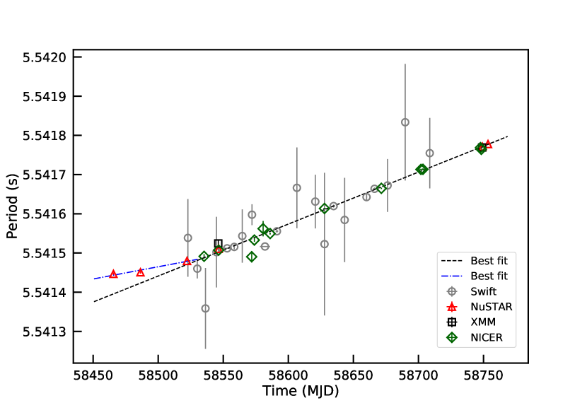
Figure 1: Values for the spin period along the 2018 outburst of XTE J1810–197 as measured in the single X-ray observations. Grey circles, red triangles, black squares and green diamonds are the measurements for Swift, NuSTAR, XMM–Newton and NICER pointings, respectively. The black dashed and blue dash-dotted lines indicate the best fit for all the data sets and a sub-sample between 2018 December 13 and 2019 February 7.

2.1 NuSTAR

XTE J1810 was observed by NuSTAR six times, for a total exposure time of $\sim$300 ks. NuSTAR consists of two co-aligned X-ray telescopes, which focus onto two focal plane detectors, referred to as FPMA and FPMB, sensitive to photons in the 3–79 keV energy band (Harrison et al., 2013). The calibrated timing accuracy of NuSTAR is $\sim$65 $\mu$s, after correcting for drift of the on-board clock (Bachetti et al., 2021).

For observations IDs 90410368002 and 80202013002, the small angular separation between the source and the Sun did not allow the star tracker co-aligned with the X-ray optics to provide an aspect solution. However, an approximate solution could be reconstructed using a combination of the other three star trackers available. Event files corresponding to each star tracker configuration were generated using the runsplitsc option in nupipeline. We extracted light curves and background-subtracted spectra, and created redistribution matrices and ancillary files for each event file. Then, we combined them by means of the tool addascaspec to generate the averaged files for both FPMs. For the other pointings, we applied standard analysis threads. Source counts were accumulated within a circular region with radius 50 arcsec, while background events were extracted from different regions (e.g., a circle of radius 100 arsec or an annulus with radii of 100 and 150 arcsec). We checked that the different choices for the background regions yielded consistent results in the spectral and timing analysis.

2.2 XMM–Newton

XMM–Newton observed XTE J1810 twice, on 2019 March 4 and September 22, with the European Photon Imaging Cameras (EPIC) for a total exposure time of $\sim$70 ks. The EPIC-pn (Strüder et al., 2001) was set in timing mode (TM; timing resolution of 0.03 ms) during the first pointing and in small window mode (SW; 5.7 ms) for the second one. For both observations, the MOS1 camera was operating in full frame mode (timing resolution of 2.6 s) while the MOS2 in timing mode (1.75 ms; Turner et al., 2001). These pointings were coordinated with NuSTAR in order to probe the magnetar emission over a broader energy range due to XMM–Newton high sensitivity to soft X-rays (0.3–10 keV). In this work, we considered only data acquired with the EPIC-pn camera, because it provides the spectra with the highest counting statistics owing to its larger effective area.

Raw data were processed via the epproc task. We cleaned the observations from any particle flares collecting light curves above 10 keV and employing an intensity threshold. In the first observation, we collected source photons from a strip with width of 11 pixels and background counts far away from the source within a strip with width of 2 pixels (1 pixel = 4.1 arcsec). While in the second pointing, the source events were selected from a 40-arcsec radius circle and the background was extracted from a source-free circular region of radius 60 arcsec. Following standard analysis procedure, the response matrices and ancillary files were generated through the rmfgen and arfgen tools, respectively.

2.3 Swift

XTE J1810 was monitored by the X-ray Telescope (XRT; Burrows et al., 2005) on board Swift, for a total exposure of $\sim$50 ks. The single exposure times ranged from 0.4 to 4.6 ks, with the XRT operating either in windowed timing (WT; 1.77 ms) or photon counting modes (PC; 2.51 s).

We reprocessed the data adopting standard cleaning criteria and created exposure maps with the task xrtpipeline. For the spectral analysis, we selected events with grades 0–12 and 0 for PC and WT data, respectively, while we extended the timing analysis to events with grades 0–2 for WT data sets. We accumulated the source counts from a circular region with radius 20 pixels (1 pixel = 2.36 arcsec). To evaluate the background in PC data, we extracted the events within an annulus centred on the source position with radii of 40 and 80 pixels. For the WT data, we adopted a region far from the target and of the same size as that used for the source. In case an observation performed in PC mode was affected by pile-up, we followed the online analysis thread to determine the size of the core of the point-spread function to be excluded from our analysis. We generated the spectra with the corresponding ancillary response files through xselect and the xrtmkarf tool. The response matrices version ‘20131212v015’ and ‘20130101v014’ available in the XRT calibration database were assigned to each spectrum in WT and PC mode, respectively.

2.4 NICER

NICER was installed on the International Space Station in June 2017 (Gendreau et al., 2012). The payload, the X-ray Timing Instrument (XTI), consists of 56 co-aligned collimators that allow X-rays in the 0.2–12 keV range onto paired silicon drift detectors. The 52 functioning detectors provide an effective area of $\sim$1900 cm² at 1.5 keV. NICER combines good energy resolution ($\sim$100 eV at 1 keV) with an excellent timing resolution ($<$300 ns), being thus the perfect instrument to perform spectral and timing studies.

NICER extensively monitored XTE J1810 from the beginning of the mission till 2018 July. When the latest outburst took place, the source was in a Solar constrained period. Observations resumed in 2019 February and covered the whole year. We included only observations with an exposure time longer than 1 ks in our analysis, for a cumulative exposure of 90.5 ks. The data were processed via the nicerdas pipeline, with the tool nicerl2 and using standard filtering criteria. Since NICER does not provide imaging capabilities, the background count rate and spectra are computed from NICER observations of the RXTE blank-field regions using the nibackgen3C50 tool. The response matrix ‘20170601v002’ and ancillary file ‘20170601v004’ were assigned to the background-subtracted spectra with the grppha task.

3 X-ray analysis and results

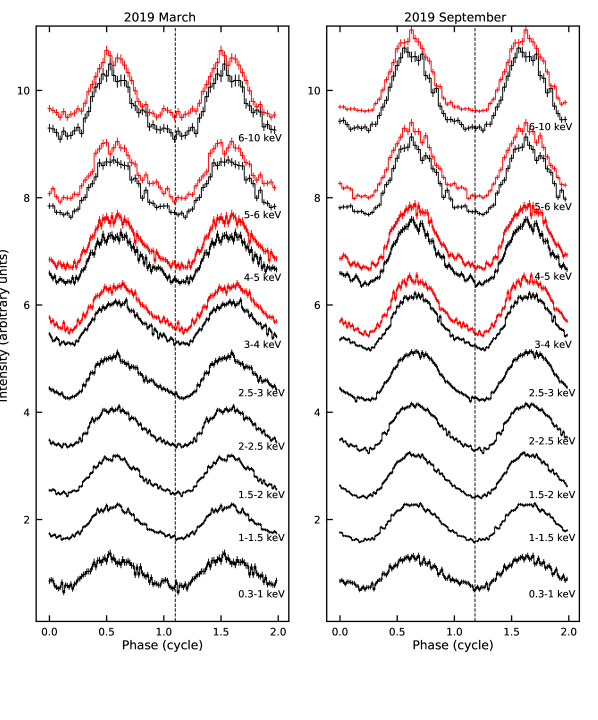
Figure 2: Energy-resolved background-subtracted pulse profiles from XMM–Newton (black) and NuSTAR (red) data sets for 2019 March (left) and September (right). The dashed lines indicate the minimum of the 0.3–1 keV pulse profiles in the two cases.

3.1 Timing analysis

In order to study the evolution of the spin period during the outburst decay, we selected events in the 0.3–10 keV energy band for XMM–Newton and Swift, 0.6–7 keV for NICER and 3–10 keV for NuSTAR. For the latter, we combined the FPMA and FPMB event files for each observation. Observations performed a few days apart were merged to increase the source signal-to-noise ratio (see Table 1).

We initially extrapolated the timing solution provided by Güver et al. (2019), who used NICER data covering the timespan 2019 February 07–15 (MJDs 58521.043–58529.490). The predicted spin period at the epoch of our data sets was employed as trial period in an epoch folding search technique, which gave us a more precise value of the period. Finally, we refined these values by applying a phase-fitting procedure in each observation (for more details see, e.g., Dall’Osso et al., 2003). Within each pointing, we were able to align the pulse phases using only a linear function. The periods derived following these steps are plotted as a function of time in Figure 1. In order to constrain the long-term average spin-down rate, we fit the period evolution with a first order polynomial function obtaining a slope of 1.5(3) $\times$ 10^-11 s s^-1. This value is consistent within 1$\sigma$ with the period derivative derived during the first three years of the 2003 outburst with the same technique (Pintore et al., 2016), and a factor of $\sim$5 higher than the value measured in quiescence (2.84(2) $\times$ 10^-12 s s^-1; Pintore et al. 2019).

A phase-coherent timing solution was reported for the initial phase of the outburst in the radio band with a baseline of $\sim$50 days, from 2018 December 8 till 2019 January 24 (see Table 1 in Levin et al., 2019). We tried to phase-connect all the observations, but this task was not possible due to the large timing noise. In order to compare the radio measurement, $\dot{P}$=7.91(1) $\times$ 10^-12 s s^-1, with our results, we modeled the period temporal evolution between 2018 December 13 and 2019 February 7 with a linear function, deriving a spin-down rate of (7.2$\pm$1.5) $\times$ 10^-12 s s^-1, value close to the radio estimate. By fitting the rest of the measurements, we obtained a spin-down rate of $\sim$1.5 $\times$ 10^-11 s s^-1, consistent with the long-term average spin-down we derived from the entire monitoring campaign and roughly twice as large as the value inferred from the first months of the outburst (see §5).

By folding each light curve at its measured spin period, we obtained the pulse profile and found that it remained single-peaked in all observations (see Figure 2). We modelled all the pulse profiles with a combination of a constant plus two sinusoidal functions, with periods fixed to those of the fundamental and first harmonic ($F$-test probability $>10^{-3}$ for the inclusion of the second sinusoidal component). We studied the dependence of the pulsed fraction (PF) with the photon energy and its evolution along the outburst decay. The PF was computed by dividing the value of the semi-amplitude for the fundamental sinusoidal component describing the pulse profile by the average count rate. Between 2018 December and 2019 October, the PF increased by a factor of $\sim$2 (from $\sim$27% to $\sim$54%) in the 3–10 keV energy interval. Moreover, the PF showed an increase as a function of energy in every observation (see Figure 3, left panel) and as a function of time in the same energy band. Figure 3, right panel, shows the pulse phase of the fundamental component as a function of energy for (quasi-)simultaneously NuSTAR, XMM–Newton and NICER observations. We clearly detected the slippage in phase reported in Gotthelf et al. (2019), with a magnitude of $\sim$0.1 phase cycles in the first four epochs and $\sim$0.05 in the last one. While in the 0.3–3.5 keV band, the pulse phase increased with energy by $\sim$0.1 cycles in 2019 March and $\sim$0.04 in 2019 September.

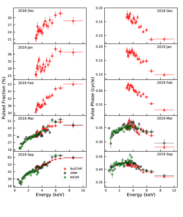
Figure 3: Pulsed fraction (left) and pulse phase of the fundamental component (right) as a function of energy for NuSTAR observations (red triangles) and the (quasi-)simultaneous XMM–Newton (black squares) and NICER (green diamonds) pointings. We note that due to the lack of a phase-connected timing solution, the pulse profiles are not aligned with each others.

Table 2: Results of the joint fit with a 3BB model of the XMM–Newton and NuSTAR spectra extracted from the nearly simultaneous observations performed on 2019 March and September (see Section 3.2).

Epoch	$kT_{\rm cold}$	$R_{\rm cold}$	$kT_{\rm warm}$	$R_{\rm warm}$	$kT_{\rm hot}$	$R_{\rm hot}$	$\chi_{\nu}^{2}$/dof
	(keV)	(km)	(keV)	(km)	(keV)	(km)
2019 Mar	0.26$\pm$0.01	5.4$\pm$1.1	0.702$\pm$0.004	1.9$\pm$0.3	1.83$\pm$0.07	0.07$\pm$0.01	1.07/613
2019 Sep	0.22$\pm$0.01	5.6$\pm$1.2	0.669$\pm$0.004	1.4$\pm$0.2	1.48$\pm$0.08	0.08$\pm$0.01

Notes. The derived absorption column density was $N_{\rm H}$ = (8.7$\pm$0.3)$\times 10^{21}$  cm^-2.

Table 3: Results of the joint fit with a 4BB model of the XMM–Newton and NuSTAR spectra extracted from the nearly simultaneous observations performed on 2019 March and September (see Section 3.2).

Epoch	$kT_{\rm cold}$	$R_{\rm cold}$	$kT_{\rm warm}$	$R_{\rm warm}$	$kT_{\rm hot}$	$R_{\rm hot}$	$\chi_{\nu}^{2}$/dof
	(keV)	(km)	(keV)	(km)	(keV)	(km)
2019 Mar	0.26$\pm$0.01	5.9$\pm$1.1	0.699$\pm$0.004	1.9$\pm$0.3	1.81$\pm$0.08	0.07$\pm$0.01	1.06/613
2019 Sep	0.25$\pm$0.01	4.5$\pm$0.9	0.669$\pm$0.004	1.4$\pm$0.2	1.49$\pm$0.05	0.07$\pm$0.01

Notes. The temperature and the radius of one BB were fixed to the values of the quiescent component, $R_{\rm NS}$ = 12.8 km and $kT_{\rm NS}$ = 0.144 keV (Bernardini et al., 2009). The derived absorption column density was $N_{\rm H}$ = (9.7$\pm$0.2)$\times$10²¹ cm^-2.

Table 4: Results of the fit with a 4BB model of the NuSTAR spectra (see Section 3.2).

Epoch	$kT_{\rm warm}$	$R_{\rm warm}$	$kT_{\rm hot}$	$R_{\rm hot}$	Flux	$\chi_{\nu}^{2}$/dof
	(keV)	(km)	(keV)	(km)	(10-11 erg s-1cm-2)
2019 Jan	0.66$\pm$0.01	2.6$\pm$0.4	1.49$\pm$0.05	0.16$\pm$0.03	14.5$\pm$0.5	1.1/146
2019 Feb	0.68$\pm$0.01	2.4$\pm$0.4	1.50$\pm$0.06	0.14$\pm$0.03	13.5$\pm$0.4	0.99/139
2019 Mar	0.63$\pm$0.01	2.5$\pm$0.4	1.38$\pm$0.06	0.17$\pm$0.04	11.5$\pm$0.2	0.99/131
2019 Sep	0.64$\pm$0.01	1.6$\pm$0.3	1.40$\pm$0.05	0.09$\pm$0.02	4.9$\pm$0.1	1.1/118

Notes. Two BB component parameters were frozen to $R_{\rm NS}$=12.8 km, $kT_{\rm NS}$=0.144 keV, $kT_{\rm cold}$=0.26 keV and $R_{\rm cold}$=5.9 km. The absorption column density was fixed at $N_{\rm H}$=9.7$\times$10²¹ cm^-2. The flux is the observed flux estimated in the 0.3–10 keV energy range.

3.2 Phase-averaged spectral analysis

We binned the NuSTAR and XMM–Newton energy spectra to guarantee at least 100 background-subtracted counts per bin. The Swift/XRT background-subtracted spectra were grouped according to a minimum number of counts variable from observation to observation, varying between 20 and 50 counts per spectral bin, while for NICER spectra we adopted 500 background-subtracted counts per bin.

The spectral analysis was performed using Xspec (version 12.10.1f; Arnaud, 1996). Once the best fit for the adopted model was found, the observed and unabsorbed fluxes were estimated with the convolution model cflux. Photoelectric absorption by the interstellar medium was included using the Tbabs model with photoionization cross-section from Verner et al. (1996) and chemical abundances from Wilms, Allen & McCray (2000).

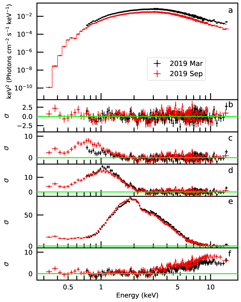
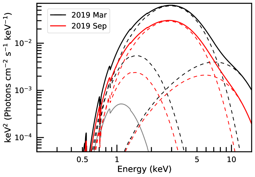
Figure 4: Top: The broad-band $E^{2}f(E)$ unfolded spectra of XTE J1810 from the simultaneous XMM–Newton and NuSTAR observations performed in 2019 March (black) and September (red). The best-fitting 4BB models are plotted with a solid line (see Sec. 3.2 for more details). Post-fit residuals in units of standard deviations are shown in Panel b. Panel c: Post-fit residuals after setting the normalization of the BB component accounting for the whole NS to zero. Panel d: Post-fit residuals after setting the normalization of the cold BB component to zero. Panel e: Post-fit residuals after setting the normalization of the warm BB component to zero. Panel e: Post-fit residuals after setting the normalization of the hot BB component to zero. Bottom: The $E^{2}f(E)$ plot of the fitted models, with the contributions of the single components. In grey, we plot the BB component that accounts for the emission from the whole stellar surface.

Firstly, we fit the XMM–Newton and NuSTAR spectra, extracted from nearly simultaneous observations, performed on 2019 March 4 and September 22–28. For the first XMM–Newton pointing, we limited the fitting energy range to 0.7–9 keV, where events are optimally calibrated for the EPIC-pn in timing mode. While for the second one, the range was extended to 0.3–10 keV. Both observations provided high-statistical-quality spectra where systematic calibration uncertainties are important. Therefore, we added an energy independent systematic uncertainty of 2% to each spectral channel2. For NuSTAR spectra, we limited the analysis to the 3–15 keV energy range because of the very low signal-to-noise ratio of XTE J1810 above 15 keV. Following Bernardini et al. (2009), we applied a three-blackbody spectral model (3BB; bbodyrad in Xspec), assuming that one of the thermal components could be identified with the emission from the whole neutron star surface. We fit the spectra jointly, including a renormalization constant to account for cross-calibration uncertainties between the two instruments. All parameters of the 3BB model were left free to vary between the two different epochs except for the hydrogen column density $N_{\rm H}$, which was forced to maintain the same value in all spectra. The fit gave an overall satisfactory description with $N_{\rm H}$ = (8.7$\pm$0.3)$\times 10^{21}$ cm^-2 and a reduced chi-squared $\chi_{\nu}^{2}$=1.07 for 613 degrees of freedom (dof). The best-fitting values relative to this model are listed in Table 2. We note that the inferred parameters for the coldest BB component, $R_{\rm cold}$$\sim$5.5 km and $kT_{\rm cold}$$\sim$0.24 keV, are different from the values estimated by Bernardini et al. (2009) for the thermal emission from the whole neutron star surface ($R_{\rm NS}\sim$12.8 km and $kT_{\rm NS}\sim$0.144 keV). This result hints at the presence of a new cold component during the latest outburst, besides the hot and warm ones. In order to investigate further this hypothesis, we fit the spectra with a 4BB model. The parameters of the additional BB component were frozen at $R_{\rm NS}$=12.8 km and $kT_{\rm NS}$=0.144 keV, as derived for the previous outburst (Bernardini et al., 2009). This component accounts for the emission from the entire stellar surface and we are assuming that it is not affected by the outburst, as it occurred during the 2003 event. The fit yields $N_{\rm H}$ = (9.7$\pm$0.2)$\times 10^{21}$ cm^-2 ($\chi_{\nu}^{2}$=1.06 for 613 dof). The best-fitting values are listed in Table 3, where the NuSTAR results refer to the data acquired with the FPMA. We repeated all the analysis using the FPMB spectra and the results were compatible within the uncertainties with those reported in Table 3. Figure 4, top panel, shows the 2019 March and September spectra with the best-fitting 4BB model, the residuals with respect to this model and the residuals after setting to zero the normalization of each BB component to highlight the contribution of each spectral component to the source spectrum.

In the following, we study in detail all the NuSTAR observations performed during this first outburst stage. The NuSTAR spectra start from 3 keV, we then decided to fix the $N_{\rm H}$, $R_{\rm NS}$ and $kT_{\rm NS}$ at the values derived in Table 3. Moreover, we kept the radius and temperature of the cold BB component frozen at the values derived from the simultaneous, broad-band fit of XMM–Newton and NuSTAR data (see Table 3). For the three NuSTAR spectra relative to pointings carried out before 2019 March, we fixed $R_{\rm warm}$ and $kT_{\rm warm}$ at the values obtained for the 2019 March data set, assuming the cold BB component to be constant through the first $\sim$80 days of the outburst.

The first NuSTAR pointing performed soon after the radio re-activation of the source (ID.90410368002, epoch: 2018 Dec) was already presented by Gotthelf et al. (2019). We reanalysed it in a consistent way with our approach. Source emission was detected up to $\sim$30 keV. The 4BB model revealed structured residuals above $\sim$15 keV, therefore an extra component was required to describe the detected hard tail. The addition of a power law (PL) to the 4BB model provided a good description of the data with $\chi_{\nu}^{2}$=0.9 for 135 dof. Best-fitting parameters were: $kT_{\rm warm}$=0.59$\pm$0.02 keV, $R_{\rm warm}$=3.5$\pm$0.6 km, $kT_{\rm hot}$=0.96$\pm$0.06 keV, $R_{\rm hot}$=0.66${}^{+0.24}_{-0.17}$ km, and photon index $\Gamma$=2.1$\pm$0.3. We note that Gotthelf et al. (2019) fitted a different model to this spectrum over the range 3–30  eV (i.e., a BB+2PL model), deriving a hard power-law photon index of $\Gamma_{h}\sim$ –0.3 for the PL characterizing the non-thermal emission, which becomes dominant above $\sim$20 keV. The four following NuSTAR observations were acquired between January and September 2019. The spectral analysis was limited to the 3–15 keV energy interval because of the very low source signal-to-noise ratio above 15k̇eV. The spectra were well-fitted by the 4BB model, with no need of the extra PL component required at the outburst peak. The fading of the non-thermal component during the outburst decay is typically observed in magnetar outbursts (e.g., Rea et al., 2009). The best-fit parameters are reported in Table 4. During the first year of the outburst decay, we can already notice a softening of the source emission from the XMM–Newton and NuSTAR data, except for the BB component which accounts for the whole surface emitting region with parameters fixed at the quiescent values ($kT_{\rm NS}$=0.144 keV and $R_{\rm NS}$=12.8 km). The $kT_{\rm cold}$ and $kT_{\rm warm}$ do not show significant variability, while $kT_{\rm hot}$ cools from $\sim$1.5 keV to $\sim$1.4 keV. Finally, we measure a shrinking for all the three regions.

To study the evolution of the hot BB component, we consider the results derived from the fit of the four NuSTAR spectra from 2019 January till September with a 4BB model, applying the procedure explained above. In particular, we note that when fitting together the March 2019 XMM–Newton and NuSTAR data, the value of the $kT_{\rm hot}$  is not compatible with that derived from fitting the NuSTAR data sets, nor it is compatible with the cooling of such component. To check further on this issue, we did several tests: a) looked at the spectrum using only PATTERN=0 events, and b) extracted the MOS2 (Timing Mode) spectrum, and fit it simultaneously with the NuSTAR spectrum. The PATTERN restriction did not change the fit parameters, however when using the MOS2 spectrum the best-fitting parameters for the hot BB component for the 2019 March epoch were $kT_{\rm hot}$=1.68$\pm$0.07 keV and $R_{\rm hot}$=0.07$\pm$0.02 km. The derived temperature is lower that what we found using the EPIC-pn (Timing Mode) data (Table 3). We then ascribe the small difference between the March 2019 value of $kT_{\rm hot}$  in Table 3 and Table 4 to uncertainties in the cross-calibration between NuSTAR  and the EPIC-pn in Timing Mode. We used the values derived by fitting the NuSTAR  long-term monitoring to study the cooling in time of the hot component.

To study the source evolution in time we also added the Swift/XRT and the NICER observations. The Swift/XRT spectra were fit in the 0.8–10 keV energy band for WT mode observations owing to known calibration issues at lower energies and in the 0.3–10 keV interval for PC mode data sets, whereas in the NICER pointings the source signal-to-noise ratio was higher in the 0.6–7 keV energy range. To increase the photon statistics, we merged observations carried out a few days apart after verifying that no significant flux variations were present (see Table 1). We hence focused on 26 Swift/XRT WT spectra, 5 Swift/XRT PC spectra and 14 NICER spectra. For consistency, we fit all the data sets with a 4BB model, where $N_{\rm H}$ and $R_{\rm cold}$ were held fixed at the values of the XMM–Newton+NuSTAR spectra closer in time, and $kT_{\rm hot}$ at the values derived from the NuSTAR spectra (Table 4). The temporal evolution of the spectral parameters is shown in Figure 5. The bottom panel of Figure 5 shows the observed flux corresponding to the 4BB model as a function of time in the 0.3–10 keV energy range. The first observation performed on 2018 December 13 caught the source at a flux of (2.2$\pm$0.3)$\times 10^{-10}$ erg s^-1cm^-2, a factor of $\approx$415 greater than the quiescent value recorded by ROSAT in 1993, (5.3$\pm$0.5)$\times 10^{-13}$ erg s^-1cm^-2 (Coti Zelati et al. (2018); see also Table 3 by Gotthelf et al. (2004)). During the following $\sim$320 days, the flux decreased slowly and reached a value of (5.2$\pm$0.2)$\times 10^{-11}$ erg s^-1cm^-2 on 2019 October 25, which is still about two orders of magnitude above quiescence.

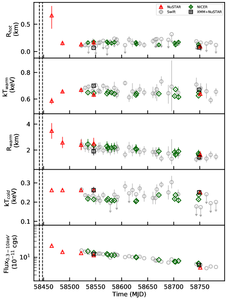
Figure 5: Temporal evolution of the free spectral parameters for the absorbed 4BB model (for details see Section 3.2). BB radii are evaluated for an observer at infinity and a distance of 2.5 kpc. The bottom panel shows the temporal evolution of the observed flux in the 0.3–10 keV energy band. The dashed vertical lines denote the range of the outburst onset as constrained by Gotthelf et al. (2019), 2018 November 20–26 (MJD 58442–58448).

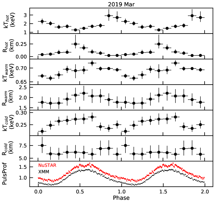
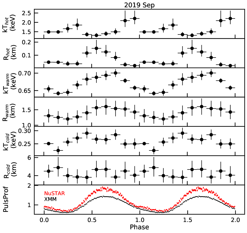
Figure 6: Phase evolution of the cold, warm and hot thermal components for the (quasi-)simultaneous XMM–Newton+NuSTAR observations performed in 2019 March (left) and September (right), with the corresponding pulse profiles (bottom panel). For plotting purpose, the NuSTAR profiles have been shifted along the vertical axis and two phase cycles are shown.

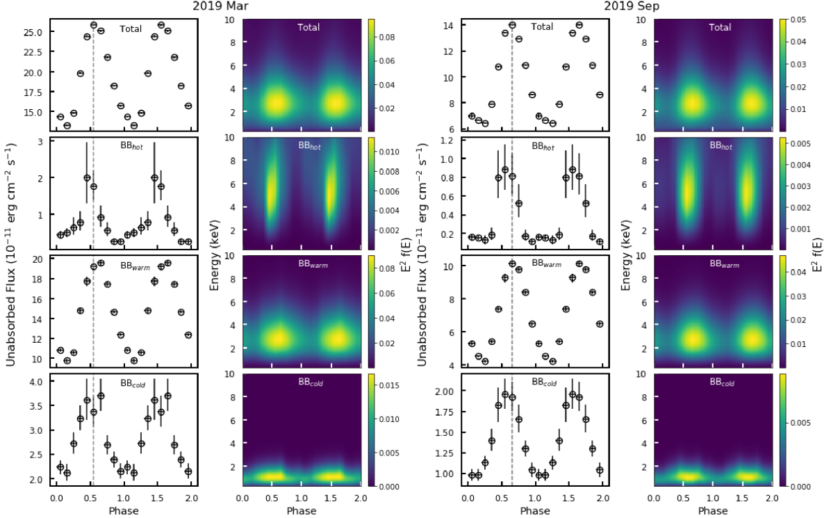
Figure 7: Dynamic spectral profiles for 2019 March (left) and September (right) observations. For each data set, the first column shows the 0.3$-$10 keV unabsorbed flux for the total model, and hot, warm, and cold blackbody components (from top to bottom). The second column shows the contour plots in the phase-energy plane for the total, hot, warm, and cold blackbody $E^{2}f(E)$ flux. The colour scale is in units of keV² (photons cm^-2 s^-1 keV^-1).

3.3 Phase-resolved spectroscopy and dynamic spectral profiles

We then carried out a pulse-phase resolved spectroscopic analysis of the (quasi-)simultaneous XMM–Newton and NuSTAR observations performed in 2019 March and September. The phase cycle was divided into 10 phase intervals in order to rely on a large enough number of photons. The phase-resolved spectra were fit simultaneously with the 4BB model. The column density was held fixed at the phase-averaged value ($N_{\rm H}$ = 9.7 $\times$ 10²¹ cm^-2; see Section 3.2). The radius and the temperature for the BB component accounting for the emission from the whole neutron star were frozen at $R_{\rm NS}$=12.8 km and $kT_{\rm NS}$=0.144 keV, while all the other parameters were allowed to vary. The fits gave $\chi_{\nu}^{2}$=1.04 for 1907 dof for the 2019 March data set and $\chi_{\nu}^{2}$=1.01 for 1719 dof for the 2019 September spectra. We found a variability of all the free parameters through the whole cycle, as shown in Figure 6.

To examine the spectral variation as a function of the star rotational phase, we produced the Dynamic Spectral Profiles (DSPs), shown in Figure 7, for both epochs. The DSPs show the contour plots of the $E^{2}f(E)$ flux as a function of phase and energy, derived from the 10 phase-resolved spectra extracted as explained above. The top panel refers to the total flux, obtained from the 4BB model, while the panels below display the flux of the single thermal components ($BB_{\rm hot}$, $BB_{\rm warm}$, $BB_{\rm cold}$).

From the DSPs and the evolution of the unabsorbed flux as a function of phase (see Figure 7), it is evident that the $BB_{\rm hot}$ component appears to be shifted in phase with respect to the total and the $BB_{\rm warm}$ emission for both epochs.

3.4 Bursting behaviour

We searched for short bursting activity in the XMM–Newton, NuSTAR and NICER observations. Four short $\sim$1 s X-ray bursts were previously reported by Woods et al. (2005), in the months following XTE J1810’s 2003 outburst. These bursts were characterized by short spikes of $\sim$1 s followed by extended tails of 100 s of seconds on enhanced flux. We find that there is no evidence of similar short bursts of this type in the data sets analyzed in this paper. Bursting activity has also been recently reported by Pearlman et al. (2020) searching through NICER data from observations between MJDs 58520 and 58540. Pearlman et al. (2020) reported on thousands of smaller bursts, with widths less than or equal to one rotational cycle, using a ‘zero crossing’ algorithm, rather than flux enhancement above the mean rate. We searched for this bursting activity in each XMM–Newton, NuSTAR and NICER observation, by calculating the mean pulse profile for each observation, and computing the differences between each individual X-ray pulse and the mean pulse profile. We grouped these count rate differences together according to rotational phase, in order to look for changes in flux from the mean flux at a given rotational phase. Then, at each rotational phase, we compared the distribution of the differences in counts with the expected distribution from Poisson sampling. We find that the differences in count rates are consistent with Poisson fluctuations.

4 Simultaneous radio observations

We observed XTE J1810 with the Sardinia Radio Telescope (SRT, Bolli et al. 2015; Prandoni et al. 2017) on 2019 February 8 for 3.6 hr starting at UT 08:01:40 (Project ID 08-19), simultaneously with NuSTAR. Data were recorded with the ATNF digital backend Pulsar Digital Filter Bank (PDFB), in search mode over a usable bandwidth of 924 MHz centered at 6.5 GHz, with a spectral resolution of 1 MHz. Full Stokes data were 2-bit sampled every 0.5 ms.

The data were folded over 1024 time bins using the ephemeris obtained from the NuSTAR simultaneous observation, showing bright pulsed emission, as it was also reported e.g., by Levin et al. (2019) for various frequencies between 1.4 and 8.4 GHz. A waterfall plot of the integrated pulse profile over the entire observing bandwidth is shown in Figure 8 (bottom), and the single peaked profile, with a $\sim 200$ ms width, is plotted at the top. The optimized signal-to-noise ratio of the pulse $\rm S/N=1066$ implies a flux density of $\sim 2.5$ mJy, assuming an antenna gain of $0.6$ K/Jy and a system temperature of $\sim$30 K. The estimated flux density is about three times lower than the value derived by Levin et al. (2019) on 2019 January 24. The radio emission was bright enough that the pulses were visible above the noise at every rotation. A snapshot of 100 subsequent single pulses stacked in phase, is plotted in the inset of Figure 8. The vast majority of single pulses are detected within the phase range of the main peak, but a minority ($<$ 1%) appears about 0.1 earlier in rotational phase. A very dim precursor of the main peak can indeed be seen in the waterfall plot. Single de-dispersed pulses show multiple narrow components with a high degree of linear polarization, as it had been also seen by e.g., Serylak et al. (2009) at 1.4, 4.8 and 8.4 GHz. No X-ray bursts were detected simultaneously with any of the radio pulses nor at any time during the 2019 February NuSTAR observation. Moreover, we compared the phase alignment of the X-ray and radio pulse profiles. We found that the X-ray peak lags the radio one by $\sim$0.08 cycles, behaviour consistent with that observed at the peak of this outburst (Gotthelf et al., 2019) and during the 2003 outburst (Camilo et al., 2016).

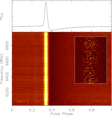
Figure 8: Frequency versus rotational phase (bottom) for the integrated pulse profile (top) of the 3.6 hr SRT observation. The dispersion delay is removed. The inset shows a subset of 100 single pulses plotted in the phase range 0.31 to 0.37.

5 Discussion

We have presented the evolution of the spectral and timing properties of the magnetar XTE J1810 during its second outburst which started in November 2018, about fifteen years after its discovery outburst in 2003. Our monitoring campaign covered the first $\sim$320 days of the outburst decay, allowing us to characterise accurately the behaviour of the source over a long time-span. In the last observation, performed on 2019 October 25 ($\sim$11 months after the outburst onset), the observed 0.3–10 keV flux was (5.2$\pm$0.2)$\times$10^-11 erg s^-1cm^-2, still two orders of magnitude higher than the historical quiescent level measured in archival ROSAT data taken in 1993 (Coti Zelati et al., 2018; Gotthelf et al., 2004).

5.1 Light curve modelling

To study the 0.3–10 keV luminosity decay, we adopt a simple phenomenological model which consists of a combination of a constant and an exponential function:

$$L(t)=L_{\rm q}+(L_{\rm max}-L_{\rm q})\exp{(-(t-t_{0})/\tau)},$$ (1)

where $L_{\rm q}$ is the quiescent luminosity, $L_{\rm max}$ is the luminosity at the outburst peak, $t_{0}$ is the onset time of the outburst and $\tau$, the $e$-folding time, can be considered as an estimate of the decay timescale. We fixed $L_{\rm q}$ to the quiescent level derived by Coti Zelati et al. (2018) from the ROSAT observation performed in 1993 and scaled for the new distance measurement, (1.3$\pm$0.1)$\times 10^{34}$ erg s^-1. The onset of the outburst was constrained to be between 2018 November 20–26 (MJD 58442–58448; Gotthelf et al., 2019) and we assumed the mid epoch, 2018 November 23 (MJD 58445), as $t_{0}$. Therefore, only ($L_{\rm max}-L_{\rm q}$) and $\tau$ were allowed to vary in the fit. A 10 per cent error was assigned to each luminosity. The best-fitting values are ($L_{\rm max}-L_{\rm q}$)=(2.1$\pm$0.1)$\times 10^{35}$ erg s^-1 and $\tau$=223$\pm$11 d. We computed the energy released in the outburst by integrating the best-fitting model for the light curve over the whole duration of the event. Our decay fit predicts that the source will reach a luminosity level consistent with the quiescent value around 2022 January, releasing a total energy of $\sim$4$\times 10^{42}$ erg. This value is estimated assuming no change in the decay pattern and, hence, should be considered only as a rough estimate. Figure 9 shows the long-term light curve of XTE J1810, spanning from 2003 September till 2019 October. The source underwent a previous outburst in 2003, whose onset was missed and is constrained to be between 2002 November 14 and 2003 January 23 (MJD 52595$-$52662; Ibrahim et al., 2004). A monitoring campaign started on 2003 September, and the first observation caught XTE J1810 at a luminosity level of $\sim 9.5\times$10³⁴ erg s^-1, a factor of $\sim$7 higher than the pre-outburst level. At the 2018 outburst onset, the luminosity reached a value of $\sim$2.5$\times$10³⁵ erg s^-1, slightly higher than what was measured in the previous outburst and a factor of 20 above the historical minimum. After $\sim$320 days, the luminosity decreased till $\sim$6$\times$10³⁴ erg s^-1, a factor $\sim$5 higher than the quiescent level.

5.2 Interpretation of the data with a physical model

During the monitoring campaign, XTE J1810 showed a thermal spectrum modelled by an absorbed four-blackbody model, apart from the first observation performed close to the outburst onset when a power-law tail was detected up to $\sim$30 keV ($\Gamma$=2.1$\pm$0.3). One of the blackbody component accounts for the emission coming from the whole neutron star and its parameters are fixed at the values inferred from the ROSAT spectra when the source was in quiescence, $kT_{\rm NS}$=0.144 keV and $R_{\rm NS}$=12.8 km (see e.g., Bernardini et al., 2009, and references therein). Besides this last component, we identified three thermally emitting areas on the star. After an initial decrease, the radius of the hot component $R_{\rm hot}$ settled to a constant value of $\sim$0.1 km; whereas the temperature $kT_{\rm hot}$ cooled from $\sim$1.5 keV to $\sim$1.4 keV (see Table 4). As shown in Figure 5, the warm region shrunk from $R_{\rm warm}$$\sim$2.6 km till $\sim$1.5 km during the $\sim$320 days of monitoring, while the corresponding temperature attained a value in the range 0.6$-$0.7 keV. For the cold area, the temperature $kT_{\rm cold}$ did not show variability and the radius $R_{\rm cold}$ decreased from $\sim$6 km to $\sim$4.5 km (see Table 3).

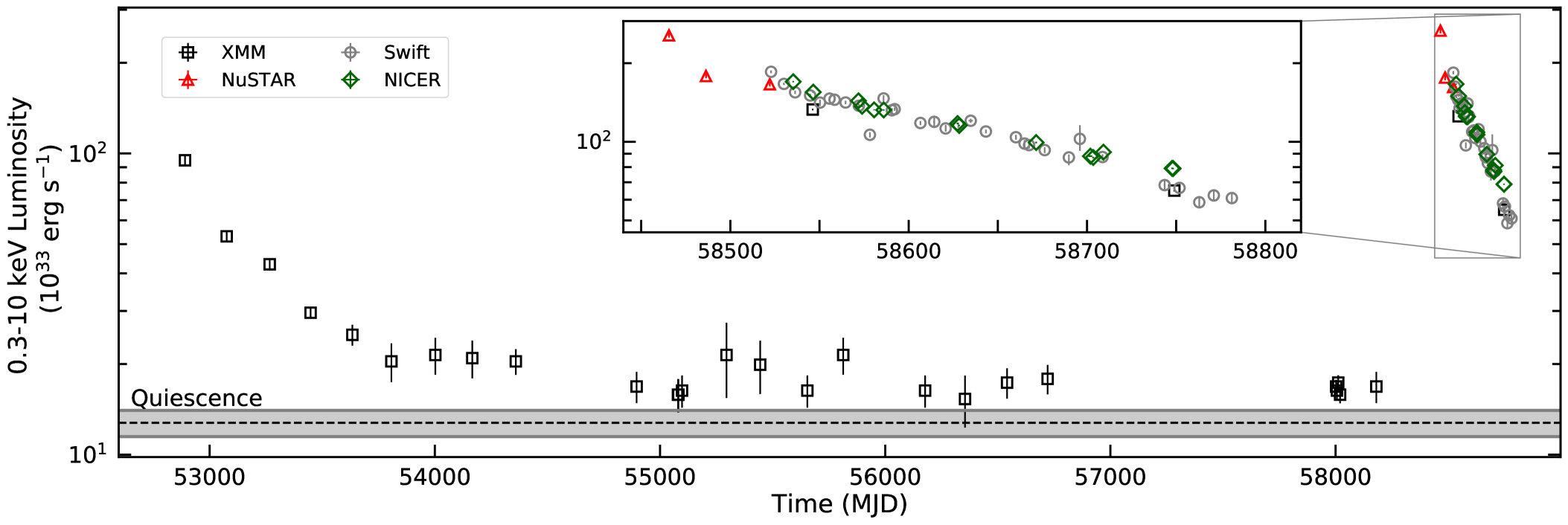
Figure 9: Long-term evolution of the 0.3–10 keV luminosity of XTE J1810 from XMM–Newton (black squares), NuSTAR (red triangles), Swift (grey circles) and NICER (green diamonds) data acquired between 2003 September and 2019 October. The solid black line denotes the quiescent level (1.3$\times 10^{34}$ erg s^-1) derived by Coti Zelati et al. (2018) from the ROSAT observation performed on 1993 April 3 and scaled for the new distance measurement. The grey area represents the associated uncertainty. The inset is a zoom of the 2018 outburst.

The simplest scenario one can envisage for the geometry of the emitting region consists of three circular, concentric, zones, superimposed to the colder star surface: a hot cap at $kT_{\rm hot}$, surrounded by a warm corona at $kT_{\rm warm}$, which is in turn surrounded by a colder ring at $kT_{\rm cold}$. This is similar to the picture adopted by Bernardini et al. (2009), although only two thermal components, a hot and a warm one in addition to emission from the entire surface, were needed in the 2003 outburst (see also Albano et al., 2010). At the peak of the 2003 event, the hot and warm regions reached lower temperatures than those measured during the 2018 outburst ($kT_{\rm warm}$₂₀₀₃ $\sim$ 0.3 keV and $kT_{\rm hot}$₂₀₀₃ $\sim$ 0.7 keV). Moreover, the size of the hot/warm areas varied during the 2003 outburst, showing a steady decrease, while the temperatures remained nearly constant.

Besides these differences, observations suggest that the emission geometry in the 2018 outburst was indeed more complex. As discussed in section 3.1 (see in particular Figure 3), in fact, the pulsed fraction (PF) increases with increasing energy and, even more relevant, the phase of the maximum of the pulse profile also changes with energy. The magnitude of this phase variation is typically $\sim 5$–$10\%$ and depends on the epoch, but the general trend always exhibits an increase up to $\approx 3$ keV, followed by a decrease. Three concentric caps can not produce such a behaviour since the phase of the maximum is always the same at different energy bands, irrespective of the viewing geometry.

In order to check if a simple, geometrical model can reproduce the observations, we consider again blackbody emission from three regions, but allowing the relative positions of the three caps to vary. The caps are taken to be circular and at constant temperature. Furthermore, we restrict ourselves to the case in which the two hotter caps are inside the cooler one (other cases can be also dealt with). The rest of the surface is at temperature $kT_{\mathrm{N}S}=0.14$ keV. The model parameters are the cap angular semi-apertures, temperatures (these are fixed by the observed blackbody values for a star radius of $13$ km) and the relative positions with respect to the axis passing through the centres of the cold cap and of the star; these are expressed through the two pairs of angles $\theta_{\mathrm{hot,warm}}$ and $\phi_{\mathrm{hot,warm}}$. In addition, there are two angles which fix the overall geometry, $\chi$ and $\xi$, between the line-of-sight and the spin axis and the cold cap axis and the rotation axis, respectively (see Figure 10).

We computed phase-resolved spectra using the method described in Turolla & Nobili (2013), which includes general-relativistic ray-bending; the star mass and radius are $M_{\mathrm{NS}}=1.4\,M_{\odot}$ and $R_{\mathrm{NS}}=13$ km. The variation of the phase of the pulse profile maximum with the energy is shown in Figure 11 for a given viewing geometry ($\xi=10^{\circ}$, $\chi=80^{\circ}$), fixed meridional cap shifts ($\theta_{\mathrm{hot}}=5^{\circ}$, $\theta_{\mathrm{warm}}=-5^{\circ}$) and different values of $\phi_{\mathrm{hot}}$ and $\phi_{\mathrm{warm}}$.

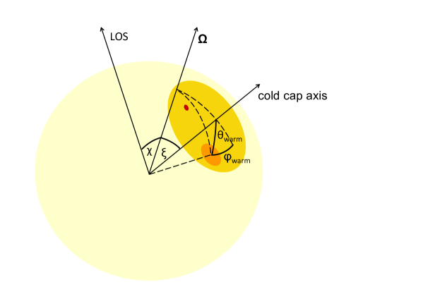
Figure 10: Schematic representation of the surface map of XTE J1810 depicting the different thermal emitting regions: the non-concentric hot (red) and warm (orange) caps, inside the cool one (yellow), superimposed to the colder star surface. The two angles fixing the warm cap position, $\theta_{\mathrm{warm}}$ and $\phi_{\mathrm{warm}}$, are shown, together with the two geometrical angles $\xi$ and $\chi$; here $\mathbf{\Omega}$ is the spin axis.

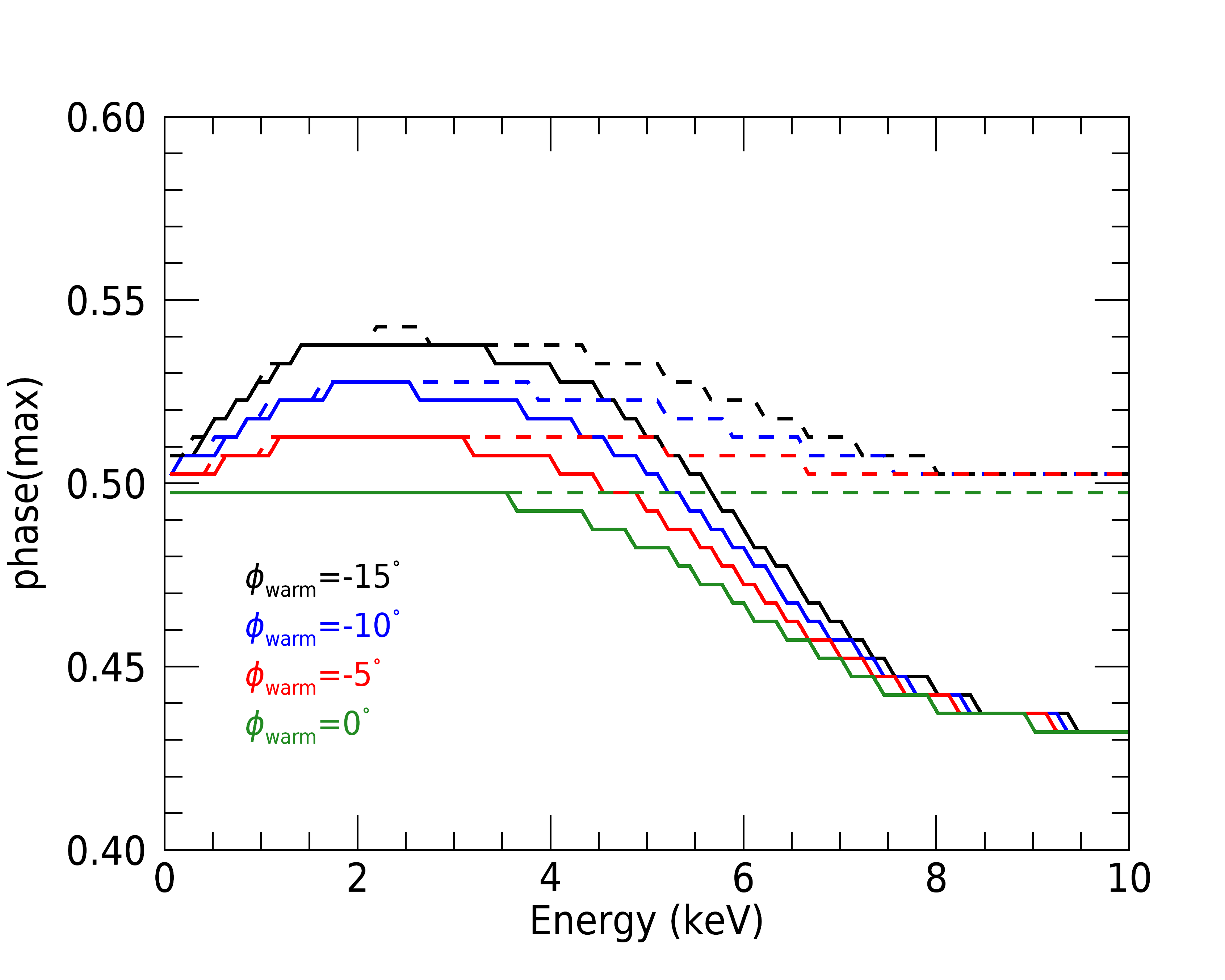
Figure 11: Phase of the maximum of the pulse profile vs. energy (at infinity) for different values of the azimuthal displacement of the hot and warm caps. The full lines are for $\phi_{\mathrm{hot}}=25^{\circ}$ and the dashed ones for $\phi_{\mathrm{hot}}=0^{\circ}$. See text for details.

The observed trend and amplitude of variation is indeed recovered, provided that the hot cap precedes the warm one ($\phi_{\mathrm{hot}}>0$ and $\phi_{\mathrm{warm}}<0$); if the signs are switched the curve has a minimum in place of a maximum. This behaviour is quite independent on both the assumed values of the meridional shifts and of the angles $\xi$ and $\chi$ and convincingly shows that the thermal structure of the heated region on the star surface is asymmetric. Actually, the modulation of the blackbody temperatures with rotational phase (see section 3.3 and Figure 6) is indicative of more complex thermal map, possibly a single heated region with a (continuous) temperature variation across it, of which our three-temperature model is just an approximation. Indeed, the appearance of such (asymmetric) thermal configurations in response to impulsive energy deposition in the star crust was been recently predicted using 3D simulations (De Grandis et al., 2020).

The geometry of the thermal emission of XTE J1810 during the 2003 outburst has been studied by various authors (Perna & Gotthelf, 2008; Albano et al., 2010; Bernardini et al., 2011). These works derived similar values of $\xi\sim 23^{\circ}$, while $\chi$ was either $\sim 53^{\circ}$ or $\sim 148^{\circ}$. We computed pulse profiles for our model at different energies, assuming the same parameter values discussed above, with $\phi_{\mathrm{hot}}=23^{\circ}$ and $\phi_{\mathrm{warm}}=-15^{\circ}$, but for all possible combinations of the two angles $\xi$ and $\chi$. The pulse profiles are quasi-sinusoidal and single-peaked. Results for the PF are shown in Figure 12 where the constant PF contours are plotted for a (red-shifted) energy of $0.6$ keV. The white lines mark the loci where the predicted PF matches the measured values for the 2019 March observation at $0.6$ (full), $2.5$ (dashed) and $4.2$ keV (dash-dotted). The PF indeed increases with energy, as expected since harder photons come from a smaller area. Clearly, the observed values of the PF in the different bands should be reproduced for the same ($\xi$, $\chi$) pair for the model to work, i.e. there should be at least one point in the plot of Figure 12 where the three lines intersect. This condition is not exactly met in the present case, although there is an indication that small $\xi$ ($\sim 10^{\circ}$) and large $\chi$ ($\sim 80^{\circ}$), or the opposite, can provide the correct answer. In this respect we note that our analysis is meant to provide an idea rather than a detailed fit to observations and, as such, contains a number of approximations. Besides the inherent simplification of assuming a three temperature cap instead of a realistic temperature map, we did not take into account the detector response function nor atmospheric effects or radiative bending in computing the pulse profiles. Moreover, all measurement errors were neglected, nor we attempted a complete exploration of the model parameter space. Finally, we remark that, if our estimate of the geometrical angles is viable, the region on the star surface of XTE J1810 involved in the 2018 outburst was likely different from that of the 2003 event.

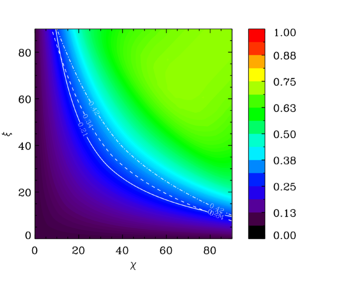
Figure 12: Pulsed fraction as a function of the two geometrical angles $\xi$, $\chi$ for a (red-shifted) energy of $0.6$ keV. The white lines mark the loci where the predicted PF matches the measured values for the 2019 March observation at $0.6$ (full), $2.5$ (dashed) and $4.2$ keV (dash-dotted). See text for details.

5.3 Timing anomalies and spin-down torque variations

Regarding the timing properties, the pulse profile attained a single-peak shape as observed in quiescence and in the 2003 outburst (see e.g., Pintore et al., 2016, 2019, and references therein). During the first $\sim$320 days of the outburst decay, the 0.3–10 keV pulsed fraction increased from $\sim$27% to $\sim$54%. This trend is opposite to that measured during the previous outburst, when the pulsed fraction decreased from $\sim$50% till $\sim$20% over 4 years, but not unusual within the magnetar population (e.g., the pulsed fraction of SGR 0418+5729 increased for $\sim$900 days since the outburst onset; Rea et al., 2013). The different evolution of the pulsed fraction with time also points to a different affected region with respect to the previous outburst (as discussed above).

Given the timing solution derived by Pintore et al. (2019) during the quiescent phase prior to the 2018 outburst, we can extrapolate the spin period of XTE J1810 at the epoch of the first NuSTAR observation. We found that the predicted period is larger than the measured value ($\Delta P$ $\sim$2$\times$10^-5 s). This discrepancy might have been caused by the occurrence of a glitch at the time of the (unobserved) outburst onset. Gotthelf et al. (2019) calculated a glitch magnitude of $\Delta\nu$/$\nu$ = (4.52$\pm$0.15)$\times$10^-6, a value typical of magnetars (Dib & Kaspi (2014); see also, e.g., Swift J1818.0$-$1607 (Hu et al., 2020)). Moreover, we found evidence of spin-down variations during our monitoring campaign: the period derivative measured during the first two months of the outburst decay ($\dot{P}\sim$7.2$\times$10^-12 s s^-1) is a factor of $\sim$2.5 higher than the value in quiescence ($\dot{P}\sim$2.8$\times$10^-12 s s^-1) and a factor of $\sim$2 smaller than the value derived for the rest of its first year evolution ($\dot{P}\sim$1.5$\times$10^-11 s s^-1). This behaviour has already been witnessed in XTE J1810 after the 2003 outburst and appears to be a common feature following magnetar outbursts (e.g., 1E 1048.1–5937; Archibald et al., 2020). Spin-down rate variations associated with outbursts are commonly explained in terms of the untwisting bundle scenario, according to which outbursts are most likely driven by magnetic stresses resulting in twistings of the external magnetic field with the formation of current-carrying localized bundles (Beloborodov, 2009). During the early stage of the outburst, the twist grows, leading to an increase in the number of (open) magnetic field lines crossing the light cylinder and, thus, to a stronger spin-down torque acting on the star. If the twist amplitude is large ($\gtrsim$1 rad), this effect should start immediately after the twist is implanted. While, if the initial twist amplitude is $<$1 rad, the spin-down torque may not be affected until the amplitude reaches 1 rad, which takes time. In this context, the delayed increase in the spin-down torque of XTE J1810 during its recent outburst (with the maximum occurring about 1.5 month after the outburst onset) would be consistent with the progressive growth of a relatively small magnetospheric twist along the early outburst phases. The presence of a limited twist is also supported by the very short appearance of a spectral power-law tail, which was observed only in the early phase of the outburst. At later stages, when the magnetosphere untwists, the spin-down torque is expected to decrease back to the value measured during the quiescent state.

6 Conclusions

We studied the long-term evolution of the X-ray emission properties of the magnetar XTE J1810 during the first year of its second outburst since its discovery in 2003. During the monitoring campaign, the source showed a thermal spectrum, apart from the outburst peak when a non-thermal tail was detected up to $\sim$30 keV. A softening of the source emission is evident during the first $\sim$320 days of the outburst decay: the observed 0.3–10 keV flux decreased from $\sim$2$\times$10^-10 erg s^-1cm^-2 to $\sim$5$\times$10^-11 erg s^-1cm^-2, about two orders of magnitude higher than the historical minimum. We also reported on the timing properties of XTE J1810. The pulse profile always showed a sinusoidal shape and the pulsed fraction increased by a factor of $\sim$2 over $\sim$300 days. At a given epoch, we found that the pulsed fraction increases with energy and the phase of the maximum of the pulse profile also changes with energy. Moreover, we measured spin-down torque variations along the outburst decay. This behaviour and the temperature distribution inferred from the spectral analysis support the scenario in which the outburst is related to the formation and gradual dissipation of a localised twisted bundle of magnetic field lines, analogous to the Solar coronal loops. Finally, we studied the geometry of the emission regions. Observational results hint to the presence of three areas, superimposed to the colder star surface. We considered a scenario according to which there are a hot and a warm cap, which are non-concentric, surrounded by a cooler one. The slippage of the phase with energy is recovered if the hot cap precedes the warm one. In this framework, the observed increase of the pulsed fraction with energy suggests that the source is a nearly aligned rotator seen almost equator on.

Data availability

The data underlying this article are public.

References

- Albano et al. (2010) Albano A., Turolla R., Israel G. L., Zane S., Nobili L., Stella L., 2010, ApJ, 722, 788
- Alford & Halpern (2016) Alford J. A. J., Halpern J. P., 2016, ApJ, 818, 122
- Archibald et al. (2016) Archibald R. F., Kaspi V. M., Tendulkar S. P., Scholz P., 2016, ApJ, 829, L21
- Archibald et al. (2020) Archibald R. F., Scholz P., Kaspi V. M., Tendulkar S. P., Beardmore A. P., 2020, ApJ, 889, 160
- Arnaud (1996) Arnaud K. A., 1996, in Jacoby G. H., Barnes J., eds, Astronomical Society of the Pacific Conference Series Vol. 101, Astronomical Data Analysis Software and Systems V. p. 17
- Bachetti et al. (2021) Bachetti M., et al., 2021, ApJ, 908, 184
- Beloborodov (2009) Beloborodov A. M., 2009, ApJ, 703, 1044
- Bernardini et al. (2009) Bernardini F., et al., 2009, A&A, 498, 195
- Bernardini et al. (2011) Bernardini F., Perna R., Gotthelf E. V., Israel G. L., Rea N., Stella L., 2011, MNRAS, 418, 638
- Bolli et al. (2015) Bolli P., et al., 2015, Journal of Astronomical Instrumentation, 4, 1550008
- Burrows et al. (2005) Burrows D. N., et al., 2005, Space Sci. Rev., 120, 165
- Camilo et al. (2006) Camilo F., Ransom S. M., Halpern J. P., Reynolds J., Helfand D. J., Zimmerman N., Sarkissian J., 2006, Nature, 442, 892
- Camilo et al. (2016) Camilo F., et al., 2016, ApJ, 820, 110
- Coti Zelati et al. (2018) Coti Zelati F., Rea N., Pons J. A., Campana S., Esposito P., 2018, MNRAS, 474, 961
- D’Aì et al. (2016) D’Aì A., et al., 2016, MNRAS, 463, 2394
- Dall’Osso et al. (2003) Dall’Osso S., Israel G. L., Stella L., Possenti A., Perozzi E., 2003, ApJ, 599, 485
- De Grandis et al. (2020) De Grandis D., Turolla R., Wood T. S., Zane S., Taverna R., Gourgouliatos K. N., 2020, ApJ, 903, 40
- Dib & Kaspi (2014) Dib R., Kaspi V. M., 2014, ApJ, 784, 37
- Ding et al. (2020) Ding H., et al., 2020, MNRAS, 498, 3736
- Esposito et al. (2021) Esposito P., Rea N., Israel G. L., 2021, Magnetars: A Short Review and Some Sparse Considerations. Springer Berlin Heidelberg, Berlin, Heidelberg, pp 97–142, doi:10.1007/978-3-662-62110-3_3
- Gendreau et al. (2012) Gendreau K. C., Arzoumanian Z., Okajima T., 2012, The Neutron star Interior Composition ExploreR (NICER): an Explorer mission of opportunity for soft x-ray timing spectroscopy. p. 844313, doi:10.1117/12.926396
- Gotthelf et al. (2004) Gotthelf E. V., Halpern J. P., Buxton M., Bailyn C., 2004, ApJ, 605, 368
- Gotthelf et al. (2019) Gotthelf E. V., et al., 2019, ApJ, 874, L25
- Güver et al. (2019) Güver T., et al., 2019, ApJ, 877, L30
- Halpern & Gotthelf (2005) Halpern J. P., Gotthelf E. V., 2005, ApJ, 618, 874
- Halpern et al. (2005) Halpern J. P., Gotthelf E. V., Becker R. H., Helfand D. J., White R. L., 2005, ApJ, 632, L29
- Harrison et al. (2013) Harrison F. A., et al., 2013, ApJ, 770, 103
- Helfand et al. (2007) Helfand D. J., Chatterjee S., Brisken W. F., Camilo F., Reynolds J., van Kerkwijk M. H., Halpern J. P., Ransom S. M., 2007, ApJ, 662, 1198
- Hu et al. (2020) Hu C.-P., et al., 2020, ApJ, 902, 1
- Ibrahim et al. (2004) Ibrahim A. I., et al., 2004, ApJ, 609, L21
- Kaspi & Beloborodov (2017) Kaspi V. M., Beloborodov A. M., 2017, ARA&A, 55, 261
- Levin et al. (2019) Levin L., et al., 2019, MNRAS, 488, 5251
- Lyne et al. (2018) Lyne A., Levin L., Stappers B., Mickaliger M., Desvignes G., Kramer M., 2018, The Astronomer’s Telegram, 12284, 1
- Mihara et al. (2018) Mihara T., et al., 2018, The Astronomer’s Telegram, 12291, 1
- Pearlman et al. (2020) Pearlman A. B., et al., 2020, arXiv e-prints, p. arXiv:2005.08410
- Perna & Gotthelf (2008) Perna R., Gotthelf E. V., 2008, ApJ, 681, 522
- Pintore et al. (2016) Pintore F., et al., 2016, MNRAS, 458, 2088
- Pintore et al. (2019) Pintore F., Mereghetti S., Esposito P., Turolla R., Tiengo A., Rea N., Bernardini F., Israel G. L., 2019, MNRAS, 483, 3832
- Prandoni et al. (2017) Prandoni I., et al., 2017, A&A, 608, A40
- Rea et al. (2009) Rea N., et al., 2009, MNRAS, 396, 2419
- Rea et al. (2013) Rea N., et al., 2013, ApJ, 770, 65
- Rea et al. (2016) Rea N., Borghese A., Esposito P., Coti Zelati F., Bachetti M., Israel G. L., De Luca A., 2016, ApJ, 828, L13
- Serylak et al. (2009) Serylak M., et al., 2009, MNRAS, 394, 295
- Strüder et al. (2001) Strüder L., et al., 2001, A&A, 365, L18
- Turner et al. (2001) Turner M. J. L., et al., 2001, A&A, 365, L27
- Turolla & Nobili (2013) Turolla R., Nobili L., 2013, ApJ, 768, 147
- Verner et al. (1996) Verner D. A., Ferland G. J., Korista K. T., Yakovlev D. G., 1996, ApJ, 465, 487
- Wilms et al. (2000) Wilms J., Allen A., McCray R., 2000, ApJ, 542, 914
- Woods et al. (2005) Woods P. M., et al., 2005, ApJ, 629, 985